design and analysis of multidimensional data structures
TRANSCRIPT

Design and Analysis of MultidimensionalData Structures
Tesi doctoral presentada alDepartament de Llenguatges i Sistemes Informatics
de la Universitat Politecnica de Catalunya
per optar al grau deDoctora en Informatica
perAmalia Duch Brown
sota la direccio del doctorConrado Martınez Parra
Barcelona, 25 d’octubre de 2004


Aquesta tesi fou llegida el dia 9 de desembre de 2004, davant el tribunal detesi format per:
• Dr. Luc Devroye (President)
• Dr. Salvador Roura (Secretari)
• Dr. Ricardo Baeza-Yates
• Dr. Pere Brunet
• Dr. Ralph Neininger


Let no one say that I have said nothing original, at least thearrangement of the subject is new.
—Blaise Pascal: Pensees.


RESUM


iii
Aquesta tesi esta dedicada al disseny i a l’analisi d’estructures de dadesmultidimensionals, es a dir, estructures de dades que serveixen per emma-gatzemar registres K-dimensionals que solen representar-se com a punts enl’espai [0, 1]K. Aquestes estructures tenen aplicacions en diverses arees de lainformatica com poden ser els sistemes d’informacio geografica, la robotica,el processament d’imatges, la world wide web, el data mining, entre d’altres.Les estructures de dades multidimensionals tambe es poden utilitzar com aindexos d’estructures de dades que emmagatzemen, possiblement en memoriaexterna, dades mes complexes que els punts.
Les estructures de dades multidimensionals han d’oferir la possibilitatde realitzar operacions d’insercio i esborrat de claus dinamicament, a mesde permetre realitzar cerques anomenades associatives. Exemples d’aquesttipus de cerques son les cerques per rangs ortogonals (quins punts cauendintre d’un hiper-rectangle donat?) i les cerques del veı mes proper (quin esel punt mes proper a un punt donat?).
Podem dividir les contribucions d’aquesta tesi en dues parts:
1. La primera part esta relacionada amb el disseny d’estructures de dadesper a punts multidimensionals. Inclou el disseny d’arbres binaris K-dimensionals al·leatoritzats (Randomized K-d trees), el d’arbres quater-naris al·leatoritzats (Randomized quad trees) i el d’arbres multidimen-sionals amb punters de referencia (Fingered multidimensional trees).
2. La segona part analitza el comportament de les estructures de dadesmultidimensionals. En particular, s’analitza el cost mitja de les cerquesparcials en arbres K-dimensionals relaxats, i el de les cerques per rangen diverses estructures de dades multidimensionals.
Respecte al disseny d’estructures de dades multidimensionals, proposemalgorismes al·leatoritzats d’insercio i esborrat de registres per als arbres K-dimensionals i per als arbres quaternaris. Aquests algorismes produeixenarbres aleatoris, independenment de l’ordre d’insercio dels registres i despresde qualsevol sequencia d’insercions i esborrats. De fet, el comportament es-perat de les estructures produıdes mitjancant els algorismes al·leatoritzats esindependent de la distribucio de les dades d’entrada, tot i conservant la sim-plicitat i la flexibilitat dels arbres K-dimensionals i quaternaris estandard.Introduım tambe els arbres multidimensionals amb punters de referencia.Aixo permet que les estructures de dades multidimensionals puguin aprofitar

iv
l’anomenada localitat de referencia en cerques associativas altament correla-cionades.
I respecte de l’analisi d’estructures de dades multidimensionals, primeranalitzem el cost esperat de las cerques parcials en els arbres K-dimensionalsrelaxats. Seguidament utilitzem aquest resultat com a base per a l’analisi deles cerques per rangs ortogonals, juntament amb arguments combinatoris igeometrics. D’aquesta manera obtenim un estimat asimptotic precıs del costde les cerques per rangs ortogonals en els arbres K-dimensionals aleatoris.
Finalment, mostrem que les tecniques utilitzades es poden extendre facil-ment a d’altres estructures de dades i per tant proporcionem una analisi delcost mitja de cerques per rang en estructures de dades com son els arbresK-dimensionals estandard, els arbres quaternaris, els tries quaternaris i elstries K-dimensionals.

RESUMEN


vii
Esta tesis esta dedicada al diseno y al analisis de estructuras de datosmultidimensionales; es decir, estructuras de datos especıficas para almace-nar registros K-dimensionales que suelen representarse como puntos en elespacio [0, 1]K . Estas estructuras de datos tienen aplicaciones en diversasareas de la informatica como son: los sistemas de informacion geografica, larobotica, el procesamiento de imagenes, la world wide web o data mining,entre otras. Las estructuras de datos multidimensionales suelen utilizarsetambien como ındices de estructuras que almacenan, posiblemente en memo-ria externa, datos mas complejos que los puntos. Las estructuras de datosmultidimensionales deben ofrecer la posibilidad de realizar operaciones deinsercion y borrado de llaves de manera dinamica, pero ademas deben per-mitir realizar busquedas asociativas en los registros almacenados. Ejemplosde busquedas asociativas son las busquedas por rangos ortogonales (¿que pun-tos de la estructura de datos estan dentro de un hiper-rectangulo dado?) ylas busquedas del vecino mas cercano (¿cual es el punto de la estructura dedatos mas cercano a un punto dado?).
Las contribuciones de esta tesis se dividen en dos partes:
1. La primera parte esta dedicada al diseno de estructuras de datos parapuntos multidimensionales e incluye el diseno de los arboles binarios K-dimensionales aleatorizados (Randomized K-d trees), el de los arbolescuaternarios aleatorizados (Randomized quad trees), y el de los arbolesmultidimensionales con punteros de referencia (Fingered multidimen-sional trees).
2. La segunda parte contiene contribuciones al analisis del comportamientode las estructuras de datos multidimensionales. En particular, damosel analisis del costo promedio de las busquedas parciales en los arbolesK-dimensionales relajados y el de las busquedas por rango en variasestructuras de datos multidimensionales.
Con respecto al diseno de estructuras de datos multidimensionales, pro-ponemos algoritmos aleatorios de insercion y borrado de registros para losarboles K-dimensionales y los arboles cuaternarios que producen arbolesaleatorios independientemente del orden de insercion de los registros y de-spues de cualquier secuencia de inserciones y borrados intercalados. De he-cho, con la aleatorizacion, garantizamos un buen rendimiento esperado de lasestructuras de datos resultantes que es independiente de la distribucion de los

viii
datos de entrada, conservando la flexibilidad y la simplicidad de los arbolesK-dimensionales y de los arboles cuaternarios estandar. En esta parte pro-ponemos tambien los arboles multidimensionales con punteros de referencia,una tecnica que permite que las estructuras de datos multidimensionales ex-ploten la localidad de referencia en busquedas asociativas que se presentanaltamente correlacionadas.
Con respecto al analisis de estructuras de datos multidimensionales, comen-zamos dando un analisis preciso del costo esperado de las busquedas parcialesen los arboles K-dimensionales relajados. A continuacion, utilizamos este re-sultado como base para el analisis de las busquedas por rangos ortogonales,combinandolo con argumentos geometricos y combinatorios. Como resul-tado obtenemos un estimado asintotico preciso del costo de las busquedaspor rango en los arboles K-dimensionales relajados.
Finalmente, mostramos que las tecnicas utilizadas pueden extendersefacilmente a otras estructuras de datos y por tanto proporcionamos un analisisdel costo promedio de busquedas por rango en estructuras de datos comolos arboles K-dimensionales estandar, los arboles cuaternarios, los tries K-dimensionales y los tries cuaternarios.

ABSTRACT


xi
This thesis is about the design and analysis of point multidimensionaldata structures: data structures that store K-dimensional keys which wemay abstract as points in [0, 1]K. These data structures are present in manyapplications of geographical information systems, image processing, robotics,world wide web, or data mining among others. They are also frequentlyused as indexes of more complex data structures, possibly stored in exter-nal memory. Point multidimensional data structures must have capabilitiessuch as insertion, deletion and (exact) search of items, but in addition theymust support the so called associative queries. Examples of these queriesare orthogonal range queries (which are the items that fall inside a givenhyper-rectangle?) and nearest neighbor queries (which is the closest item tosome given point q?).
The contributions of this thesis are two-fold:
1. Contributions to the design of point multidimensional data structureswhich includes: the design of randomized K-d trees, the design of ran-domized quad trees and the design of fingered multidimensional searchtrees;
2. Contributions to the analysis of the performance of point multidi-mensional data structures: the average-case analysis of partial matchqueries in relaxed K-d trees and the average-case analysis of orthogonalrange queries in various multidimensional data structures.
Concerning the design of randomized point multidimensional data struc-tures, we propose randomized insertion and deletion algorithms for K-d treesand quad trees that produce random K-d trees and quad trees independentlyof the order in which items are inserted into them and after any sequence ofinterleaved insertions and deletions. The use of randomization provides ex-pected performance guarantees, irrespective of any assumption on the datadistribution, while retaining the simplicity and flexibility of standard K-dtrees and quad trees.
Also related to the design of point multidimensional data structures is theproposal of fingered multidimensional search trees, a new technique that en-hances point multidimensional data structures to exploit locality of referencein associative queries.
With regards to performance analysis, we start by giving a precise analysisof the cost of partial matches in randomized K-d trees. We use these results

xii
as a building block in our analysis of orthogonal range queries, together withcombinatorial and geometric arguments and we provide a tight asymptoticestimate of the cost of orthogonal range search in randomized K-d trees. Wefinally show that the techniques used apply easily to other data structures,so we can provide a precise analysis of the average cost of orthogonal rangesearch in other data structures such as standard K-d trees, quad trees, quadtries, and K-d tries.

ACKNOWLEDGMENTS


xv
I once heard –possibly in a quotation by Thomas Fuller– that “couragemay triumph over uncertain questions, while only patience over desperateones”. The completion of this dissertation involved a long list of desperatesituations that I prefer not to mention here. However, I wish to express mygratitude to the many teachers, friends and family who helped and encour-aged me through their guidance, example, support and, mostly, patience.
I want to thank, specially, Conrado Martınez whose advice, unlimited pa-tience, guidance and constant encouragement (often beyond academic mat-ters) made this thesis possible. Salvador Roura, whose work is the foundationof mine. Josep Dıaz who kept a vigilant eye in my activities, facilitated finan-cial support when necessary and showed concern and encouragement whenI needed them most. Rafel Cases who was my tutor when I first arrivedto the UPC and started me in the analysis of algorithms. And VladimirEstivill-Castro who introduced me to computer science and to research.
I would also like to thank those who over the years have given me theirfriendship, but they are too numerous to mention all of them here. I do,however, want to express special thanks to a few whose presence, criticismand encouragement were directly involved with this dissertation. Carme andAna who have always been so close to me deserve a particular mention.Following them are: Edelmira, Ma. Amelia, Fatos, Nicola, Miguel, Balqui,Adriana, Rosa, Ma. Jose, Ma. Luisa, Xavier, Javier, Jordi P., Jordi M., JuanLuis, Cristina, Christian, Cora, Vianey, Luz Elena, Elena, among too manyothers.
Finally, I want to thank my family. My parents above all, my brothers andin-laws and with a special word, Pablo and Ximena who loved me throughthe tough and wonderful experience of writing and delivering this thesis.
Funding. I received financial support from CONACyT (Mexico) undergrant number 89422 and travel support from the Future and Emergent Tech-nologies Program of the EU under contract IST-1999-14186 (ALCOM-FT)and the Spanish Min. of Science and Technology project TIC2002-00190(AEDRI II) to present parts of this dissertation.


CONTENTS
Part I Introduction 1
Part II Preliminaries 9
1. The Associative Retrieval Problem . . . . . . . . . . . . . . . . . . 111.1 Multidimensional Data . . . . . . . . . . . . . . . . . . . . . . 121.2 Associative Retrieval . . . . . . . . . . . . . . . . . . . . . . . 16
2. Hierarchical Multidimensional Data Structures . . . . . . . . . . . . 192.1 Basic Multidimensional Data Structures . . . . . . . . . . . . 202.2 Data Structures Based on K-d Trees . . . . . . . . . . . . . . 242.3 Data Structures Based on Quad Trees . . . . . . . . . . . . . . 322.4 Other Hierarchical Multidimensional Data Structures . . . . . 35
Part III Design of Multidimensional Data Structures 39
3. Randomized Relaxed K-d Trees . . . . . . . . . . . . . . . . . . . . 413.1 Relaxed K-d Trees . . . . . . . . . . . . . . . . . . . . . . . . 433.2 Randomized K-d Trees . . . . . . . . . . . . . . . . . . . . . . 463.3 The Split and Join Algorithms . . . . . . . . . . . . . . . . . . 493.4 Properties of Randomized K-d Trees . . . . . . . . . . . . . . 52
4. Randomized Quad Trees . . . . . . . . . . . . . . . . . . . . . . . . 574.1 Quad Trees . . . . . . . . . . . . . . . . . . . . . . . . . . . . 584.2 Randomized Quad Trees . . . . . . . . . . . . . . . . . . . . . 614.3 Properties of Randomized Quad Trees . . . . . . . . . . . . . 67
5. Fingered Multidimensional Trees . . . . . . . . . . . . . . . . . . . 735.1 Finger K-d Trees . . . . . . . . . . . . . . . . . . . . . . . . . 74

xviii Contents
5.2 Locality Models and Experimental Results . . . . . . . . . . . 81
Part IV Analysis of Multidimensional Data Structures 99
6. Mathematical Preliminaries . . . . . . . . . . . . . . . . . . . . . . 1016.1 Generating Functions . . . . . . . . . . . . . . . . . . . . . . . 1026.2 Singularity Analysis . . . . . . . . . . . . . . . . . . . . . . . . 104
7. Analysis of Partial Match Queries . . . . . . . . . . . . . . . . . . . 1097.1 The Partial Match Algorithm . . . . . . . . . . . . . . . . . . 1107.2 The Cost of Partial Match Searches . . . . . . . . . . . . . . . 113
8. Analysis of Orthogonal Range Queries . . . . . . . . . . . . . . . . 1198.1 The Cost of Range Searches . . . . . . . . . . . . . . . . . . . 1208.2 Other Multidimensional Data Structures . . . . . . . . . . . . 1298.3 A Note on Nearest Neighbor Search . . . . . . . . . . . . . . . 1308.4 Experimental Results . . . . . . . . . . . . . . . . . . . . . . . 130
Part V Conclusions and Future Work 137
Appendix 143
A. Plots of Fingered Multidimensional Trees . . . . . . . . . . . . . . . 145
B. Analysis of Orthogonal Range Queries with Random Corners . . . . 159

It is interesting to note that the human brain is much better atsecondary key retrieval than computers are; in fact, people find itrather easy to recognize faces or melodies from only fragmentaryinformation, while computers have barely been able to do this atall. Therefore it is not unlikely that a completely new approach tomachine design will someday be discovered that solves the prob-lem of secondary key retrieval once and for all, making this entiresection obsolete.
—Donald E. Knuth: The Art of Computer Programming,Second Edition, Volume 3: Sorting and Searching (1999).


Part I
INTRODUCTION


3
This thesis is about the design and analysis of multidimensional datastructures, a field that has been in constant growth in the last decade due tothe increasing popularity of applications that naturally require it, like websearching, geographical information systems, image processing, or robotics,among others [43, 95].
By multidimensional data we understand data that is usually representedin some vector-based form. Consequently, multidimensional data structuresare data structures specifically designed for the storage and management ofmultidimensional data. In the literature, multidimensional data structuresare also referred to as multidimensional access methods, spatial access meth-ods or spatial index structures [43].
Within multidimensional data structures it is important to distinguishbetween point data structures and spatial data structures. Point data struc-tures are multidimensional data structures that maintain a collection of itemsor records, each holding a distinct K-dimensional key (which we may assumew.l.o.g. is a point in [0, 1]K). Spatial data structures store more complexspatial objects such as lines, polygons or higher dimensional polyhedra.
In this thesis we devote our attention to point data structures1, not onlybecause many applications involve them, but because it is not uncommon torepresent more complex spatial data and even complex non-spatial objects,such as multimedia files or text documents, as multidimensional points gen-erally called surrogates. Surrogates are frequently used in order to createindexes of complex data, in such a way that many of the required manipula-tions can be performed in simpler elements (the surrogates) and consequentlybecome more efficient. Moreover, it is often the case that large data basesare stored in external memory while all the accesses are made through theindexes via the surrogates. In what follows we will use the term multidi-mensional data structures to refer to point multidimensional data structures,unless otherwise stated.
Retrieval (or search) in multidimensional data structures is usually knownas associative retrieval. Besides insertions, deletions, and (exact) search, amultidimensional data structure should allow efficient answers to questionslike which records of the data structure do fall within a given hyper-rectangleQ (orthogonal range search) or which is the closest record to some givenpoint q according to some distance or similarity metric (nearest neighbor
1 But many of the techniques we use in this work can be applied also to other kinds ofmultidimensional data structures.

4
search) [43, 95], to mention a few.The design of multidimensional data structures must take into account the
intrinsic properties of multidimensional data and their applications. Specif-ically, multidimensional data is dynamic, since applications involve series ofinterleaved insertions, deletions, and associative queries, multidimensionaldata tend to be large, the set of requirements depends strongly on the par-ticular application, and in general, associative operations are more expensivethan standard ones. As stated by V. Gaede and O. Gunther [43],
“the challenge for the developers of a spatial database systemlies not so much in providing yet another collection of special-purpose data structures. Rather, one has to find abstractionsand architectures to implement generic systems, that is, to buildsystems with generic spatial data-management capabilities thatcan be tailored to the requirements of a particular application do-main”.
With this goal in mind, we focused our attention in K-d trees [4] andquad trees [6], two basic general-purpose multidimensional data structuresthat are widely used in applications because they support a large set of asso-ciative queries with reasonable space and time requirements. One of the maindrawbacks of these hierarchical structures is that their performance dependson the randomness of the inputs. Furthermore, the existing deletion algo-rithms do not preserve randomness, so that the overall performance of thesedata structures may degrade significantly after long sequences of interleavedinsertions and deletions [21, 32].
In order to overcome these problems, we have proposed randomized K-d trees and randomized quad trees. These new data structures are fullydynamic (in the sense that they support insertions and deletions in any orderwith the guarantee that their expected time bounds hold), they efficientlysupport a broad range of associative queries, they are simple to describe andimplement, and they work for any dimension.
We obtained these results through theoretical and experimental analysisof the proposed data structures. In particular, a noteworthy contributionof this thesis is our mathematical analysis of the performance of orthog-onal range queries for randomized K-d trees, which is actually applicableto a broad collection of multidimensional data structures. In general, theaverage-case analysis of the performance of orthogonal range queries for mul-tidimensional data structures has proven to be a difficult problem. The orig-

5
inal analysis for standard K-d trees by Bentley et al. and most subsequentwork [4, 99] rely on the unrealistic assumption that the considered tree datastructure is perfectly balanced, and thus, provide unduly optimistic results.Progress came with two papers [14, 24] that provide upper (Ω) and lowerbounds (big-Oh) for the average performance of range search in standardK-d trees, squarish K-d trees, and other multidimensional data structures.
In this thesis, we analyze the average cost of range queries for a largeclass of hierarchical multidimensional data structures using the same ran-dom model as in [14, 24] but completely different techniques, and we obtainsharper results. In particular, we get exact upper and lower bounds and acharacterization of the cost of range search as the sum of the cost of par-tial match-like searches. Using these results, we provide tight asymptoticestimates for the expected cost of range search.
These new data structures, and in particular randomized K-d trees, haveattracted the attention of other researchers as witnessed by the references toour work in [14, 17, 58, 72, 78, 79].
In another line of work, we take advantage of locality of reference inmultidimensional search. Although locality of reference is systematicallyused in the design of memory hierarchies (disk and memory caches) and it isthe rationale for many other techniques like buffering and self-adjusment [11,100], it was not exploited in the case of multidimensional data. We introducea new type of data structure, the fingered multidimensional trees, whichare easy to implement and yield significant savings under reasonable modelsof orthogonal range and nearest neighbor queries that exhibit locality ofreference.
The thesis is organized as follows. Part I corresponds to this introduction.In Part II we give an overview of the field of multidimensional data structuresand the notation and basic definitions to be used later on.
The design of multidimensional data structures is the subject addressedin Part III, which includes:
1. The design of Randomized K-d Trees (Chapter 3),
2. The design of Randomized Quad Trees (Chapter 4), and
3. The design of Fingered Multidimensional Trees (Chapter 5).
In Chapters 3 and 4 we introduce randomized K-d trees and randomizedquad trees, variants of classical K-d trees [4] and quad trees [6], respec-

6
tively. Randomized K-d trees are a generalization of randomized binarysearch trees [73]. We first define relaxed K-d trees, K-d trees in which thesequence of discriminants in a path from the root to any leaf is arbitrary,contrary to standard K-d trees, where the sequence of discriminants alongany path is cyclic, starting with the first coordinate. The flexibility of relaxedK-d trees (Chapter 3) allows us to use randomization to perform insertionsand deletions in regions of the trees other than the leaves, in such a way thatthe resulting trees have all the properties of randomly built trees. Hence, theexpected case performance of every operation holds, since it only depends onthe random choices made by the randomized update algorithms.
Randomized quad trees, whose definition is similar to the one presentedabove, have other noteworthy advantages. We present and study them inChapter 4. While deletion in standard quad trees [93] depends on a specificnotion of distance and becomes more cumbersome as the spatial dimensiongrows, the randomized deletion algorithm for quad trees that we presenthere is defined for any dimension and is independent of any notion of prox-imity or distance between the stored spatial objects. The expected valuesof random variables (such as internal path length, depth, cost of successfulor unsuccessful search, cost of partial match queries, among others) given inthe literature [23, 25, 36, 70] for random quad trees are valid for randomizedquad trees, because, as for randomized K-d trees, the randomized updatealgorithms produce random quad trees.
The third proposed data structures, which we introduce in Chapter 5,the fingered multidimensional trees, have been designed with on-line settingsin mind, where requests arrive one at a time and they must be attended assoon as they arrive (or after some small delay). In such cases, we frequentlyencounter locality of reference, that is, for any time frame only a small numberof different requests among the possible ones are made or consecutive requestsare close to each other in some sense. The performance of searches andupdates in data structures can be improved by augmenting the data structurewith fingers, pointers to the hot spots in the data structure where mostactivity is going to be performed for a while (see for instance [12, 45]). Thus,successive searches and updates do not start from scratch but use the cluesprovided by the finger(s), so that when the request affects some item in the“vicinity” of the finger(s) it can be attended more efficiently.
In this work, we will concentrate in fingering techniques applied to twovariants of K-dimensional trees, namely standard K-d trees [4] and relaxedK-d trees, but the techniques can easily be applied to other multidimen-

7
sional search trees and data structures. We propose two alternative designs(1-finger and m-finger K-d trees) that augment K-d trees with fingers to im-prove the efficiency of orthogonal range and nearest neighbor searches. Wethereafter study their performance under reasonable models which exhibitlocality of reference. While it seems difficult to improve the performance ofmultidimensional data structures using self-adjusting techniques (as reorga-nizations in this type of data structures is too expensive), fingering yieldssignificant savings and is easy to implement. Our experiments show that themore complex scheme of m-finger K-d trees exploits better the locality ofreference than the simpler 1-finger K-d trees; however these gains probablydo not compensate for the amount of memory that m-finger K-d trees need,so that 1-finger K-d trees might be more attractive on practical grounds.
Part IV of the thesis is devoted to the analysis of associative queries inmultidimensional data structures. In this case, using average-case analysistechniques we provide:
1. The analysis of partial match queries in random relaxed K-d trees(Chapter 7), and
2. The average-case analysis of orthogonal range search in a large class ofhierarchical spatial data structures (Chapter 8).
Chapter 7 is devoted to the analysis of partial match queries. As shownby Flajolet and Puech [38], the expected time performance, measured as thenumber of visited nodes, for a partial match query in random K-d trees isΘ(n1− s
K+θ( s
K)), where n is the number of nodes in the tree, s is the number of
specified attributes in the query, 0 < s < K, and θ(x) is a real valued functionwhose magnitude never exceeds the value 0.07. In our work, we show that theexpected number of visited nodes in a partial match query with s specifiedattributes in a random relaxed K-d tree of size n is βn1− s
K+φ( s
K)+O(1), where
we provide the closed forms for φ and β as functions of s/K; in particularthe value of φ(x) never exceeds 0.12. The simplicity and flexibility of relaxedK-d trees is reflected also in a simpler and more complete mathematicalanalysis of partial match queries than those available for standard K-d treesand other variants [14, 17, 24, 38, 72, 79]. In particular, the exact value for βdepends only on s/K, whereas for standard K-d trees the cost of the partialmatch is also dependent on the pattern structure of the query.

8
We address, in Chapter 8, the mathematical analysis of the performanceof range searches. We analyze first the average cost of range search in ran-domized K-d trees. In our analysis we use the previous analysis of partialmatches as a building block, together with combinatorial and geometric ar-guments, to provide a tight asymptotic estimate.
In particular, let E [Rn] be the expected cost of a range search with arandom query in a random relaxed K-d tree of size n. Then we show that
E [Rn] ∼ ∆0∆1 · · ·∆K−1 · n +∑
0<j<K
cj · n1−j/K+φ(j/K)
+2 · (1 − ∆0) · · · (1 − ∆K−1) · log n + O(1),
where ∆r is the length of the range for coordinate r, and we give explicitvalues for the cj ’s. Similar results hold for the rest of the multidimensionaldata structures mentioned above, but different cj ’s and φ appear in eachinstance. This result can be used to show that, in random relaxed K-d trees,nearest neighbor queries are answered on-line in expected Θ(nρ +log n) time,where ρ = max0<s<K(φ(s/K)).
We finish the chapter by discussing how our results generalize to othermultidimensional data structures, namely, standard K-d trees, squarish K-d trees, K-d-t trees, standard and relaxed K-d tries, quad trees and quadtries [4, 6, 13, 22, 24, 89].
Finally, in Part V, we review the main conclusions of the present workproposing a brief account of some open problems raised by our research.
Chapter 3 is based on Randomized K-dimensional Binary Search Trees [27].Most of the material in Chapter 4 is presented in Randomized Insertion andDeletion in Point Quad Trees [26] and the results of Chapter 5 appear inFingered Multidimensional Search Trees [31].
The material of Chapter 7 is presented in Randomized K-dimensionalSearch Trees [27]. Chapter 8 is based on the paper On the Average Perfor-mance of Orthogonal Range Search in Multidimensional Data Structures [29,30].

Part II
PRELIMINARIES


1. THE ASSOCIATIVE RETRIEVAL PROBLEM

12 1. The Associative Retrieval Problem
1.1 Multidimensional Data
Points, lines or hyper-planes lying in Euclidean space; strings of fixed lengthlying in Hamming space; strings of variable length lying in Leveshtein space;geographic maps, books or other text documents, acoustic or musical data,proteins, are all examples of multidimensional data. Multidimensional dataobjects are present in a broad range of applications in computer sciencesuch as databases, data-mining, computer graphics, robotics, medical images,neural networks, multimedia, statistical computing, computer-aided design,astronomy, pattern recognition, geographic information systems, music in-formation retrieval, computational biology, etc. For information about thesespecific applications we refer the reader to [94] and the references therein.
In general, by multidimensional data we mean data that contain explicitinformation about objects, their extent, and/or their position in space. Thisinformation is usually represented by vectors. And it is generally assumedthat multidimensional data objects lie in a K-dimensional space which isreferred to as universe. Here K is a natural number corresponding to dimen-sionality.
An explicit example of two-dimensional geographic data is shown in Ta-ble 1.1 which lists some localities in Catalonia together with their corre-sponding latitude and longitude coordinates. Figure 1.1 shows the geographiclocalization of the listed localities.
Multidimensional data structures are multidimensional data managementsystems that support search and update operations in multidimensional data.In the literature, multidimensional data structures are also referred to as mul-tidimensional access methods, spatial access methods or spatial index struc-tures. Within multidimensional data structures it is important to distinguishbetween point multidimensional data structures and spatial multidimensionaldata structures. The point data structures are multidimensional data struc-tures that store points in two or more dimensions. Spatial data structures canstore extended spatial objects such as lines, polygons or higher dimensionalpolyhedra, among others.
Multidimensional data have basic properties that are essential in thestudy of their management systems. Specifically, spatial data have a complexstructure (because they can consist of several polygons arbitrarily distributedin space), are dynamic (since applications involve series of interleaved inser-tions, deletions and associative queries) and tend to be large (geographicmaps, for instance, can occupy some gigabytes of storage). Moreover, there

1.1. Multidimensional Data 13
Locality Longitude Latitude(A) Arenys de Mar 233′ E 4133′ N(B) Barcelona 211′ E 4123′ N(C) Cardona 149′ E 4156′ N(D) Delta de l’Ebre 045′ E 4045′ N(E) Empuries 315′ E 4220′ N(F) Figueres 258′ E 4214′ N(G) Girona 249′ E 4159′ N(H) Hostalric 245′ E 4145′ N(I) Igualada 137′ E 4135′ N(J) Jonquera 300′ E 4230′ N(L) Lleida 038′ E 4137′ N(M) Manlleu 217′ E 4200′ N(N) Nuria 213′ E 4230′ N(O) Olot 230′ E 4211′ N(P) Puigcerda 156′ E 4226′ N(Q) Querol 130′ E 4130′ N(R) Reus 106′ E 4110′ N(S) Seu d’Urgell 128′ E 4222′ N(T) Tarragona 116′ E 4107′ N(U) Ullastret 310′ E 4216′ N(V) Vic 215′ E 4156′ N(X) Xert 015′ E 4044′ N
Tab. 1.1: A two-dimensional file of localities in Catalonia.

14 1. The Associative Retrieval Problem
Fig. 1.1: Geographic representation of the Catalan localities listed in Table 1.1.

1.1. Multidimensional Data 15
is no standard set of spatial operators (since they strongly depend on theparticular application), many spatial operators are no closed (the intersec-tion of two polygons, for instance, may not be a polygon) and in general,multidimensional operators are more complicated than standard ones.
The objects of study in this thesis are point multidimensional data struc-tures. This is because multidimensional data points are frequently presentin applications and also because it is common to represent extended data (orobjects), like text documents or multidimensional files, as multidimensionalpoints generally called surrogates.
A practical example of surrogates is the representation of characters inthe 16-bit Unicode code space. For instance, the Chinese speaking commu-nity alone uses over 55,000 characters of the 65,536 that fit in the system(without surrogates). The Unicode Standard augments its character capac-ity by defining surrogates. In this case a surrogate is a pair of 16-bit Unicodecode values that represent a single character. In this way, Unicode can sup-port over one million characters. For more details we refer the reader to TheUnicode Standard System [20], version 2.0.
There are two frequent ways for assigning spatial extended objects tomultidimensional points. The first possibility is to transform each extendedobject into a higher multidimensional point [53, 97]. For example, two-dimensional rectangles can be represented as four dimensional points eithertaking the coordinates of two of their diagonal corners (end point trans-formation) or taking its centroid together with its extension in both coor-dinates (middle point transformation). The second option is to transformextended objects into a set of one-dimensional intervals by means of spacefilling curves [92]. There are several variations of the space filling curvestechnique. Examples are: z-ordering [85], the Hilbert tree [57], and the UB-tree [2].
Another important application of surrogates is that they are frequentlyused in order to create indexes of complex data. Indexes are then used toperform either simpler manipulations of the complex data objects or accessesto large multidimensional data bases stored in external memory.
In what follows, unless otherwise stated, we will use the term multidimen-sional data structures to refer to point multidimensional data structures.We also will look at points in a K-dimensional space as multidimensionalrecords. For the sake of simplicity, we identify a multidimensional recordwith its corresponding K-dimensional key x = (x0, x1, . . . , xK−1), where eachxi, 0 ≤ i ≤ K − 1, refers to the value of the i-th attribute of the key x. As

16 1. The Associative Retrieval Problem
an example, consider the file given in Table 1.1, consisting of some localitiesin Catalonia. Each record corresponds to one locality and has associatedtwo attributes: the latitude and longitude of the locality; so K = 2 in thisexample. In general, each xi belongs to some totally ordered domain Di, andx is an element of D = D0 × D1 × . . . × DK−1. Without loss of generality,we assume that Di = [0, 1] for all 0 ≤ i ≤ K − 1, and hence that D is thehypercube [0, 1]K [70]. And the file F of n multidimensional records is simplyF = x(1), x(2), . . . , x(n).
1.2 Associative Retrieval
Retrieval (or search) in multidimensional data structures is generally knownas associative retrieval (also referred to as retrieval by secondary key, re-trieval by composite key, or as multi-key retrieval). In our work associativeretrieval consists of requesting and retrieving information from a collectionof multidimensional points (or records). There is a condition imposed torequests, they must deal with more than one of the point coordinates. Ifthis condition is not satisfied and all the requests deal with only one of thecoordinates, then, one-dimensional data structures have better performancethan multidimensional ones.
Associative queries are usually divided into two groups: intersection andproximity queries. Intersection queries, in turn, are classified in exact matchqueries, partial match queries and region queries.
An exact match query is a query in which all key attributes are specified.The retrieval consists of finding all records in the file with the given key. Inthe file of Table 1.1 an exact match query could be, for instance, a request fora record with attributes 215′ E of longitude and 4156′ N of latitude (Vic).This is formally stated by the next definition.
Definition 1.2.1. Given a file F of n K-dimensional records and a K-dimensional query record q, an exact match query consists of retrieving thepoint x in F whose coordinates match the coordinates of q. This is,
x ∈ F | xi = qi, ∀i ∈ 0, . . . , K − 1.
A partial match query is a query in which only s out of the K attributesof a given key are specified (with 0 ≤ s < K). The retrieval consists offinding all the records whose specified key attributes coincide with those of

1.2. Associative Retrieval 17
the given query. Retrieving in Table 1.1 all those records with latitude equalto 4045′ N (Delta de l’Ebre) is an example of partial match query. Theformal definition is as follows.
Definition 1.2.2. Given a file F of n K-dimensional records and a queryq = (q0, q1, . . . , qK−1) where each qi is either a value in Di (it is specified) or∗ (it is unspecified), a partial match query returns the subset of records x inF whose attributes coincide with the specified attributes of q. This is,
x ∈ F | qi = ∗ or qi = xi, ∀i ∈ 0, . . . , K − 1.
Given a bit-string w, a record y ∈ D, and a partial match query q =(q0, q1, . . . , qK−1), where qi = yi if wi = 1 and qi = ∗ if wi = 0, we say that wis the specification pattern of the partial match query q.
To every partial match query with record y and specification pattern wwe associate the hyperplane H(y, w) defined by
H(y, w) = x ∈ F | ∀i : wi = 1 =⇒ xi = yi.
Notice that the value of yi in the definition of H(y, w) is irrelevant if wi = 0.For instance, if K = 2 and D = [0, 1]2, then H(y, 00) = D, H(y, 11) =
y, H(y, 01) is a line passing through y parallel to the horizontal axis andH(y, 10) is a line passing through y parallel to the vertical axis.
A region query is a more general type of query. In this case, the querydefines any region of the K-dimensional space of keys. The retrieval consistsof searching in the file for all the points that fall inside the given region.When the region query is a hyper-rectangle whose sides are orthogonal tothe coordinate axis we say that it is a range query. As an example, considera request for all those localities in Table 1.1 with longitude between 000′ Eand 100′ E and latitude between 4000′ N and 4200′ N (Delta de l’Ebre,Lleida and Xert). Formally we have the following.
Definition 1.2.3. Given a file F of K-dimensional records and a hyper-rectangle Q = [l0, u0]× [l1, u1]×· · ·× [lK−1, uK−1], an orthogonal range queryreturns the subset of records in F which fall inside Q. This is,
x ∈ F | li ≤ xi ≤ ui, ∀i ∈ 0, . . . , K − 1.
Therefore, exact match queries are region queries in which the regions areisolated points and partial match queries with s attributes specified corre-spond to the region being a (K − s)-dimensional hyper-plane.

18 1. The Associative Retrieval Problem
A request for the closest record to a given query record, under a de-termined distance function, is called a nearest neighbor query. A nearestneighbor query is, for instance, a request for the locality in Table 1.1 closestto (211′, 4123′) (Barcelona). The definition is the following.
Definition 1.2.4. Given a file F of K-dimensional records and a query pointq, a nearest neighbor query consists of finding the key in the file closest to qaccording to some predefined distance measure d. This is,
x ∈ F | d(q, x) ≤ d(q, y), ∀y ∈ F.
Nearest neighbor queries can be extended to m-nearest neighbor queries:given a query point q, it is required to find the m keys in the file closest tothe given one, according to a given distance measure.
Definition 1.2.5. Given a file F of K-dimensional records and a query pointq, a m-nearest neighbor query consists of finding the m keys in F closest toq according to some predefined distance measure d. This is,
A ⊆ F | |A| = m and for all x ∈ A, d(q, x) ≤ d(q, y), for all y ∈ F.
A request for the record(s) in the file at a distance at most δ from a givenpoint is a proximity query.
Definition 1.2.6. Given a file F of K-dimensional records, a query pointq, and a distance value δ, a proximity query consists of finding the keys inthe file with distance at most δ from q according to some predefined distancemeasure d. This is,
x ∈ F | d(q, x) ≤ δ.
This type of query can also be seen as a region query, but it shares acommon flavor with nearest neighbor queries.

2. HIERARCHICAL MULTIDIMENSIONAL DATASTRUCTURES

20 2. Hierarchical Multidimensional Data Structures
2.1 Basic Multidimensional Data Structures
Nowadays, numerous data structures and algorithms exist for handling mul-tidimensional data and associative queries, and much work is going on in thesubject [43, 60, 95]. There exist also several taxonomies for the classificationof these data structures [95, 97]. In general, they can be separated into twomain groups: the hierarchical multidimensional data structures (tree-like)and the non-hierarchical ones (mostly based on hash). Multidimensionaldata structures may reside either in main or in external memory. Since mul-tidimensional data structures tend to be very large, it is common to storedata in external multidimensional access structures and to use main memorystructures as indexes to access them [43].
In this chapter, we focus our attention in main memory hierarchical mul-tidimensional data structures not only because they are the basis of thecontributions of this thesis but because they also are the basis of the de-velopment of the field. However, we mention the original data structures inwhich are based the classes of: (a) non-hierarchical data structures and (b)hierarchical data structures lying in external memory. We do not pretend togive an exhaustive description of the existing hierarchical data structures tohandle multidimensional data, but to give a flavor of the existing techniquesand the historical development of the field in order to provide a better un-derstanding of the associative retrieval problem. The description herewithis very general and concentrates only on the main characteristics of eachmethod. We focus mainly in those hierarchical data structures that had animpact on the design of multidimensional data structures.
In some cases, in order to simplify the description of multidimensionaldata structures and the algorithms governing them, it is assumed that eachof the points to be stored is unique. In other words, that the K-dimensionalrecords to be stored are all compatible.
Definition 2.1.1. We say that two K-dimensional keys x and y are compat-ible if, for every i = 0, 1, . . . , K − 1, their i-th attributes are different.
Note that any two keys drawn uniformly and independently from [0, 1]K
are compatible, since the probability that xi = yi is zero.If an application permits collisions (i.e., several data points with the same
attribute values), then one possibility to handle this situation is to providethe data structure with an additional field in which a pointer to an overflowcollision list would be stored. In such a case, the update algorithms should

2.1. Basic Multidimensional Data Structures 21
Long. X → L → D → R → T → S → Q → I → C → P → B → N → V → M → O → A → H → G → F → J → U → ELat. X → D → T → R → B → Q → A → I → L → H → V → C → G → M → O → F → U → E → S → P → N → J
Tab. 2.1: Inverted file built from Table 1.1.
be slightly modified. It could be argued that devoting an extra field toan unfrequent event such as a collision wastes storage; however, without it,more complicated update procedures would be required. Another possibilityto solve this problem is to determine rules for handle collisions. In the case ofbinary trees, for instance, it is usual to decide arbitrarily to give preferenceto one side of the tree, lets say right. That is, if a record x to be inserted isequal to a record y already in the tree, then x should be inserted always inthe right subtree of the node containing y.
The assumption of compatibility of keys is usual in the average case analy-sis of the performance of associative queries and it will be required in Parts IIIand IV of this thesis.
The simplest and straightforward approach to associative retrieval is tostore the records in a sequential list. As a query arrives, all the elementsof the list are sequentially scanned and every record that satisfies the queryis reported. If the queries do not have to be handled immediately, then,they can be batched so that many queries can be processed with a singlesequential pass through the file. For a file of n K-dimensional records, thelist structure has the following properties; Θ(Kn) time to build the list,Θ(Kn) storage is required and associative queries are answered in Θ(Kn)(worst-case) time. Lists have the advantage of being very easy to implement.They are competitive with the more sophisticated methods described in thiswork when the file is small and the number of attributes large, or when theapplication is such that a large number of file records satisfy the query.
A natural extension to the use of lists is the projection technique (alsocalled inverted files [60]). It consists of keeping, for each attribute, a sortedsequence of the records in the file. Geometrically, this corresponds to pro-jections of the points on each coordinate. The K lists representing the Kprojections can be obtained by using K times some standard sorting algo-rithm. The inverted file corresponding to the file of Table 1.1 of localities inCatalonia1 is represented in Table 2.1.
1 In what follows we will refer to localities in the file of Table 1.1 only by its leadingcharacter.

22 2. Hierarchical Multidimensional Data Structures
To preprocess a file of n K-dimensional records we must perform K sortsof n elements, which takes Θ(Kn log n) time. To store such a file requireΘ(Kn) space. An exact match query can be answered by searching (usingbinary search) any of the K sorted lists in Θ(log n) worst-case time. Theworst-case cost for any kind of associative queries is Θ(Kn). Range queriescan be answered by the following procedure: choose one of the attributes,say the i-th. Find the two limits of the range query in the appropriatesorted sequence (using binary search). All the records satisfying the querywill be in the list between these two positions. This (usually smaller) list isthen searched by brute force. For almost cubical range queries that have asmall number of records satisfying them (and are therefore similar to nearest-
neighbor searches), the range query time of projection is given by Θ(n1− 1K )
in the average case when the point set is drawn from a smooth underlyingdistribution [8]. In solving range queries, the projection technique is mosteffective for queries containing one range that excludes most of the recordsin the file. If the distribution of attribute values is more or less uniform oversimilar ranges and the query range is cubical, then we can use the projectiontechnique with only one sorted list.
This technique has been applied by Friedman, Baskett, and Shustek [41]in their algorithm for nearest-neighbor queries, in particular they show thatnearest-neighbor queries can be answered using projection in Θ(n1− 1
K ) timeand Θ(Kn log n) preprocessing. Also Lee, Chin and Chang have appliedprojection to a number of database problems [67].
The cell or fixed grid method, first introduced by Nievergelt, Hinterbergerand Sevcik [80] and based in extendible hashing, divides the space into equalsized cells or buckets (squares and cubes for two and three dimensional datarespectively). The data structure is a K-dimensional array with one entryper cell. Each cell is implemented as a linked list storing the points withinit. In Figure 2.1 we illustrate one possible grid for Table 1.1.
The space required for this data structure can be super-linear in thenumber n of records, even if the data is uniformly distributed. In particular,Regnier [88] showed that the average size of the grid file while storing nK-dimensional records is Θ
(
n1+(K−1)/(Kb+1))
, where b is the bucket size,and that the average occupancy of the data buckets is approximately 69%.The analysis of the performance of grid files on associative queries [88] musttake two costs into account; the number of required cell accesses (or numberof directory look-ups) and the number of required inclusion tests (testing

2.1. Basic Multidimensional Data Structures 23
41
42
LAT.
0
40
LONG.32
B
C
D
G
H
M
N
Q
R
V
X
1
U
O
I A
P
J
ES
F
T
L
Fig. 2.1: Illustration of the cell method; a grid for the file in Table 1.1.
whether a point satisfies the query). If the cell size is large there will be fewcell accesses and many inclusion tests. By contrast, if the cell size is small,there will be many cell accesses and few inclusion tests. Both extremes areunsuitable.
Range queries with constant size can be answered (in a file organizedby cells having the same size than the queries) with approximately 2K cellaccesses [8]. The expected search time in this case is proportional to 2K timesthe average number of points per cell. In such files nearest neighbor querieshave similar performance. In most applications, however, the queries willvary in size and shape, and there is little information available for making agood choice of cell size (and possibly shape).
Most of the non-hierarchical multidimensional data structures are based,inspired or closely related in some way to grid files. Examples of such datastructures are: excell [102] (extendible cell), two-level grid file [53], twin gridfile [54], molhpe [61] (multidimensional order-preserving linear hashing withpartial expansions), quantile hashing [62, 64], and plop [63] (piecewise lin-ear order-preserving hashing), among others. We do not go further in thedescription of such data structures. Our interest in grid files is due to itsrelation with some of the hierarchical data structures that we explain below.

24 2. Hierarchical Multidimensional Data Structures
2.2 Data Structures Based on K-d Trees
Bentley [4] introduced multi-dimensional binary search trees (K-d trees) as ageneralization of binary search trees. A K-d tree is a combination of cells andbinary search trees in which the space is also divided into hyper-rectangles,but this time depending on the records’ attributes.
Definition 2.2.1. A K-d tree for a set F = x(1), x(2), . . . , x(n) of K-dimensional records is a binary tree such that:
1. Each node contains a K-dimensional record and has an associated dis-criminant j ∈ 0, 1, . . . , K − 1.
2. For every node with key x and discriminant j, the following invariantis true: any record in the left subtree with key y satisfies yj < xj , andany record in the right subtree with key y satisfies yj ≥ xj .
3. The root node has depth 0 and discriminant 0. All nodes at depth dhave discriminant (d mod K).
Note that we do not need to explicitly store a field containing the dis-criminant of each node, since they are implicitly given by the third conditionof the definition above.
We say that a node contains (x, j) if its key is x and its discriminant isj. Let us now give a definition that will be required later on.
Definition 2.2.2. We say that a K-dimensional key x is compatible with atree T if, ∀j ∈ 0, . . . , K − 1, its j-th attribute is different from the j-thattribute of the keys already in T .
A K-d tree for a file F can be incrementally built by successive insertionsinto an initially empty K-d tree as follows. If the tree T is empty, theinsertion of x results in a K-d tree with root node x and empty subtrees.The first attribute of the second key is then compared with the first attributeof the key at the root: if it is smaller, the second key is recursively inserted inthe (empty) left subtree; otherwise, it is recursively inserted in the (empty)right subtree. In general, when inserting a key x, we compare the key to beinserted with some key y at the root of some subtree: if y is at level j, thenwe compare x(j mod K) and y(j mod K), and recursively continue the insertionin the left or the right subtree of y, until a leaf (empty subtree) is found. In

2.2. Data Structures Based on K-d Trees 25
Figure 2.2 we show the 2-d tree that results from the insertion of the keys ofthe file in Table 1.1 into an initially empty tree, in the same order as theyhave been listed. The figure also shows the partition of the space inducedby the 2-d tree. It should be clear that if the same points were inserted in adifferent order they could yield a substantially different tree.
In discussing deletions, it is sufficient to consider the problem of deletingthe root node of a (sub)tree. If the root to be deleted (say y) has no subtrees,then the resulting tree is the empty tree. If y does have descendants anddiscriminant j (with 0 ≤ j ≤ K − 1), then it must be replaced by either thenode in its left subtree with greater j-th attribute or the node in its rightsubtree with smaller j-th attribute.
The standard model for the probabilistic analysis of K-d trees is that arandom K-d tree of size n is built by inserting n points independently drawnfrom some continuous probability distribution defined over [0, 1]K . This isequivalent to assume that the probability that the (n + 1)-th insertion failsin a given leaf of a random K-d tree of size n is the same for any of its n + 1leaves.
The expected cost of a single insertion in a random K-d tree is Θ(log n)time while the expected cost of building the whole tree is Θ(n log n) [4]. Theworst-case cost for insertions in a K-d tree is Θ(n) while the worst-case costof building a K-d tree of n nodes is Θ(n2). The cost of deleting the root of a
random K-d tree with n nodes is Θ(n1− 1K ). But in the average, deletions have
expected cost Θ(log n) since the expected depth of the node to be deleted islogarithmic and the subtree beneath it has expected size 2 log n [4, 71].
Exact match queries in random K-d trees obviously operate by followinga path down the tree, exactly in the same way as if we were inserting thatkey: either we find it and report success or we reach a leaf, reporting failure.Therefore, they also require expected Θ(log n) time and Θ(n) worst-casetime.
The algorithm for partial match searches over K-d trees explores thetree in the following way. At each node of the K-d tree it examines thecorresponding discriminant. If that discriminant is specified in the query thenthe algorithm recursively follows in the appropriate subtree, depending on theresult of the comparison between the attribute of the query and the attributeof the key at the current node. Otherwise, the algorithm recursively followsthe two subtrees. It has been shown by Flajolet and Puech [38] that partialmatch queries are efficiently supported by random K-d trees. The expected

26 2. Hierarchical Multidimensional Data Structures
A
B
D
X R
T 2
C
I
Q L
2 S
M
V N
P O
E
F
G
H 2
U
J
41
42
LAT.
0
40
LONG.32
B
C
D
G
H
M
N
R
V
X
1
U
O
A
P
J
S
F
T
Q
L I
E
Fig. 2.2: Graphic and geometric representation of a K-d tree built from Table 1.1.

2.2. Data Structures Based on K-d Trees 27
time of this operation in random K-d trees of size n is Θ(n1− sK
+θ( sK
)), wheres is the number of specified attributes, 0 < s < K, and θ(x) is a real valuedfunction whose magnitude never exceeds the value 0.07.
The algorithm for orthogonal range queries is similar to the previous one.When visiting a node x that discriminates w.r.t. the j-th coordinate, we mustcompare xj with the j-th range [ℓj, uj] of the query. If the query range istotally above (or below) that value, we must search only the right subtree(respectively, left) of that node. If, by contrast, ℓj ≤ xj ≤ uj, then bothsubtrees must be searched; additionally, we must check whether x falls or notinside the query hyper-rectangle. This procedure continues recursively untilempty subtrees are reached. The pseudo-code is presented in Algorithm 1.From now on, we use the notation p → field to refer to the field field inthe node pointed to by p. Usually, a K-d tree is represented by a pointerto its root node, and each node has three fields: key, left subtree and rightsubtree. In other variants of K-d trees (in the chapters to follow) it is alsorequired a pointer to that node’s discriminant since there is no implicit wayfor obtaining them.
Algorithm 1 The orthogonal range search algorithm for K-d trees.
function range_search(T : K-d tree, Q : query) : setif (T = nil) then return ∅;x := T → key;if (Q.u[j] < x[j]) then return range_search(T → left, Q);if (Q.l[j] ≥ x[j]) then return range_search(T → right, Q);set S := range_search(T → left, Q) ∪ range_search(T → right, Q);if (x ∈ Q) then S := S ∪ x;return S;
end
One important concept related to orthogonal range searches is that ofbounding box or bounding hyper-rectangle of a data point. In the case of K-dtrees constructed with keys taken from [0, 1]K , a bounding hyper-rectangleis defined as follows.
Definition 2.2.3. Given an item x in a K-d tree T , its bounding hyper-rectangle B(x) = [ℓ0(x), u0(x)] × . . . × [ℓK−1(x), uK−1(x)] is the region of[0, 1]K defined as follows:
1. If x is the root of T then B(x) = [0, 1]K ;

28 2. Hierarchical Multidimensional Data Structures
2. If y = (y0, . . . , yK−1) is the parent of x and it discriminates w.r.t. thej-th coordinate then,
• if xj < yj, then B(x) = [ℓ0(y), u0(y)] × . . . × [ℓj(y), yj] × . . . ×[ℓK−1(y), uK−1(y)];
• if xj ≥ yj then B(x) = [ℓ0(y), u0(y)] × . . . × [yj, uj(y)] × . . . ×[ℓK−1(y), uK−1(y)].
It can be observed that B(x) is the region of [0, 1]K that corresponds tothe leaf replaced by x when it was inserted in the K-d tree. Taking the treeand the partition of Figure 2.2, it is easy to see that the bounding box ofthe node labelled A is B (A) = [000′, 330′] × [4000′, 4300′]. Node B hasbounding box B (B) = [000′, 233′] × [4000′, 4300′], while the boundinghyper-rectangle of node E is B (E) = [000′, 233′] × [04000′, 4300′]. Thebounding hyper-rectangles of the rest of nodes can be recursively obtained.
There are several variants for nearest neighbor searching in K-d trees.One of them, which we will use in Chapter 5, works as follows. The initialclosest point is the root of the tree. Then we traverse the tree as if wewere inserting q. When visiting a node x that discriminates w.r.t. the j-th coordinate, we must compare qj with xj . If qj is smaller than xj wefollow the left subtree, otherwise we follow the right one. At each step, wemust check whether x is closer or not to q than the closest point seen sofar, and update the candidate nearest neighbor accordingly. The procedurecontinues recursively until empty subtrees are reached. If the hyper-sphere,say Bq, defined by the query q and the candidate closest point is totallyenclosed within the bounding boxes of the visited nodes then the search isfinished. Otherwise, we must visit recursively the subtrees corresponding tothose nodes whose bounding boxes intersect but do not enclose Bq. Thisis Algorithm 2 described below, where dist(x, y) is a predefined distancefunction between the keys.
It is important to note that the algorithms for partial match, orthogonalrange and nearest neighbor searches are essentially the same for any variantof K-d trees and quad trees (except for finger multidimensional trees, intro-duced in Chapter 5). The difference lies in the costs of the algorithms, whichare dependent on the specific characteristics of the data structure.
The efficient expected performance of a K-d tree holds only under theassumption that it is random. Unfortunately, in practical applications, thisassumption does not always hold. For instance, it fails when the keys to be

2.2. Data Structures Based on K-d Trees 29
Algorithm 2 Nearest neighbor search algorithm for K-d trees.
⊲ Precondition: T is not empty⊲ Initial call: NN(T, q,∞, nn)procedure NN(T : K-d tree, q : query, min dist : distance value, nn : key) : void
x := T → key;d := dist(q, x);if (d < min dist) then
min dist := d;nn := x;
if (q[j] < x[j]) then
NN(T → left, q, min dist, nn);other := T → right;
else
NN(T → right, q, min dist, nn);other := T → left;
if (q[j] − min dist ≤ x[j] and q[j] + min dist ≥ x[j]) then
NN(other, q, min dist, nn);end
inserted are sorted or nearly sorted with respect to one of the attributes.Moreover, an alternation of deletions and insertions over a random K-d treedestroys its randomness [21, 32]. This happens even if every item in the fileis equally likely to be deleted. After some updates (insertions and deletions),the tree may need to be rebuilt to preserve its efficient expected performance.
One possibility to overcome this problem is the use of optimized K-dtrees [40, 101], assuming that the file of records is given a priori. SuchK-d trees are perfectly balanced and their logarithmic depth is guaranteed.However, when insertions and deletions are to be performed, a reorganizationof the whole tree is required. Thus, this alternative is not suitable unlessupdates occur rarely and most records in the file are known in advance,conditions that are not met in many practical situations.
Another approach is to introduce explicit constraints on the balancingof the trees, as in dynamically balanced K-d trees, in divided K-d treesor in K-d-t trees [22, 103, 86]. At each step, all update operations checkwhether a predefined balance criterion remains true after the insertion or thedeletion of an element. If the balance constraint is violated then a rathercomplex reorganization of the tree is performed. Although these methodsyield theoretical efficient searches (exact search and associative queries), andin some cases provide worst-case guarantees, they sacrifice the simplicity of

30 2. Hierarchical Multidimensional Data Structures
the standard K-d tree update algorithms and might be impractical in highlydynamic environments.
An interesting variant of K-d trees are squarish K-d trees proposed byDevroye, Jabbour and Zamora-Cura [24]. Assuming that the file of recordsis known a priori, squarish K-d trees are built by choosing as discriminant ateach level the attribute with maximum spread in values, instead of assigningdiscriminants sequentially trough all the coordinates. The average cost ofpartial match queries in squarish K-d trees of n nodes is similar to the oneof perfectly balanced complete K-d trees, namely Θ(n1− s
K ), when s out ofK attributes are specified. Despite the good performance of squarish K-dtrees in partial match and other associative queries, they are unsuitable indynamic environments because insertions and deletions may force a completereorganization of the tree.
The idea of K-d trees can easily be generalized to digital search trees [13,89] making a regular partition of the search space based on digits. Therecursive partition of a region of the search space terminates when the regioncontains one (or no) data points. Searching in a binary K-d trie is as follows.At level 0 we use the first digit of the first key. If it is a zero the searchproceeds to the left of the trie, and the search proceeds to the right if thebit is a one. The first bit of the second key is used in level 1, and so on,up to level K − 1. Then, in level K we use the second bit of the first keyand so on. In general, in level j we must use the (⌊j/K⌋ + 1)-th bit of the(j mod K)-th attribute of the given key. In Figure 2.3 we depict a 2-d triefor the set of records of the file in Table 1.1 and the induced partition ofthe search space. Note that both, the tree and the partition, depend on thegiven set of keys but not in the order in which they were inserted in the trie.
The probability model for the average-case analysis of K-d tries (andother variants) is usually the Bernoulli model, in which each of the K at-tributes of a key x is an infinite string of 0’s and 1’s, each bit independentlygenerated, with identical probability (symmetric Bernoulli model) or withfixed probabilities p and 1 − p (asymmetric Bernoulli model). The perfor-mance of partial match queries in K-d tries and other multidimensional digi-tal structures (such as digital search trees or Patricia tries) is on the averageΘ(
n1−φ)
, where the coefficient, instead of being constant as in K-d trees, isa fluctuating function of the main order term [72].
We have just described K-d tree based multidimensional data structuresfor main memory storage, which are the basis of a wide range of data struc-

2.2. Data Structures Based on K-d Trees 31
•
•
•
•
•
X D
2
•
2 •
R •
T Q
•
L •
I S
•
•
B 2
•
•
•
C •
•
V A
•
M O
•
P N
•
•
•
•
H 2
•
2 •
G F
2
•
2 •
•
•
U J
E
2
41
42
LAT.
0
40
LONG.32
B
R
V
X
1
O
J
S
L
E
FM
P
Q
T
I
C
D
N
G
A
U
H
Fig. 2.3: Graphic and geometric representation of a K-d trie built from the file inTable 1.1.

32 2. Hierarchical Multidimensional Data Structures
tures for external memory. Let us mention for instance: KDB trees [90],Extended KD trees [74], BSP trees [42], BD trees [81], SKD trees [83],LSD trees [50], hB trees [69], GDB trees [82], G-trees [65], hBπ trees [33],and BV trees [39].
2.3 Data Structures Based on Quad Trees
Quad trees, introduced by Finkel and Bentley [34, 95], are also a generaliza-tion of binary search trees. In a 2-dimensional space the quad tree is givenby the next definition.
Definition 2.3.1. A quad tree for a file F = x(1), x(2), . . . , x(n) of 2-dimensional records is a quaternary tree in which:
1. Each node from F contains a 2-dimensional key and has associated foursubtrees corresponding to the quadrants NW , NE, SE and SW .
2. For every node with key x the following invariant is true: any record inthe NW subtree with key y satisfies y1 < x1 and y2 ≥ x2; any recordin the NE subtree with key y satisfies y1 ≥ x1 and y2 ≥ x2; any recordin the SE subtree with key y satisfies y1 ≥ x1 and y2 < x2; and, anyrecord in the SW subtree with key y satisfies y1 < x1 and y2 < x2.
This definition for two-dimensional quad trees is readily generalized toan arbitrary dimension K (see Definition 4.1.1 in Chapter 4). The corre-sponding quad trees will have branching factor 2K . For simplicity, most ofthe operations and properties that we describe in what follows are referredto 2-dimensional quad-trees, but they are easily generalized to higher dimen-sions.
A quad tree for a file F can be incrementally built by successive insertionsinto an initially empty quad tree as follows. The first record in the fileis inserted as the root node. The insertion of the second record consistsof comparing its attributes against the attributes of the root, in order todetermine to which subtree it corresponds. If the appropriate subtree isempty then the record is inserted at its root. Otherwise the record is insertedrecursively in the appropriate subtree. The remaining records are insertedin the same way. In Figure 2.4 we show the 2-d tree that results from theinsertion of the keys of the file in Table 1.1 into an initially empty tree, inthe same order as they have been listed. The figure also shows the partition

2.3. Data Structures Based on Quad Trees 33
induced by the quad tree. It should be clear that if the same points wereinserted in a different order they could yield a substantially different tree.
Deletion of nodes into two-dimensional quad trees is complicated. Finkeland Bentley [34] suggested that all nodes of the tree rooted at the deletednode must be reinserted, but this is usually expensive. A more efficientprocess developed by Sammet [95, 93] allows to reduce the number of nodesto be reinserted, although it is still an expensive and not straightforwardprocess (it is described in Chapter 4).
Algorithms for exact search, partial match, orthogonal range search andnearest neighbor search are similar to those for K-d trees already described.
The standard model for the probabilistic analysis of quad trees is that arandom quad tree of size n is built by inserting n points independently drawnfrom some continuous probability distribution defined over [0, 1]K .
The expected height Hn of a K-dimensional quad tree of size n is in prob-ability asymptotic to (c/K) log n, where c = 4.31107 . . . [23]. It has beenshown independently by Devroye and Laforest [25] and Flajolet et al. [35]that the expected cost of a random search in a random K-dimensional quadtree of size n − 1 is (2/K) log n. For two-dimensional random quad treesof size n − 1 Devroye and Laforest [25] show that the variance of a random
search is√
2K2 log n. A complete characterization of random searches in K-
dimensional quad trees is given by Flajolet and Lafforgue [36]. In particular,they show that the cost of a random search has logarithmic mean and vari-ance, and that it is asymptotically distributed as a normal variable, althoughno closed forms are given for K ≥ 3.
The cost of a random partial match query with s coordinates specifiedin random quad trees of size n and dimension K is Θ(n1−s/K+θ(s/K)), wherethe function θ(x) is defined as the solution θ ∈ [0, 1] of the equation (θ + 3−x)x(θ + 2 − x)1−x − 2 = 0 [35].
The range search cost in quad trees has been studied by Bentley, Stanatand Williams [7] and by Lee and Wong [66]. In particular, Lee and Wongshow that in the worst-case, range searching in a complete two-dimensionalquad tree of size n takes Θ(n1/2) time. This result can be extended to Kdimensions to yield Θ(n1−1/K) cost.
As it was the case for K-d trees, the efficient expected case performanceof quad trees is based on the assumption that the quad tree is random. Butthis assumption does not always hold in applications.
Assuming that all nodes are known a priori, Finkel and Bentley [34]

34 2. Hierarchical Multidimensional Data Structures
A
C
S M
N
2 2 2 P
O 2 2
V I
L 2 2 2
E
J 2 2 F
2 2 U G
2 2 2 H
2 B
Q 2 2 D
2 R
2 2 T 2
2 X
41
42
LAT.
0
40
LONG.32
B
D
G
R
V
X
1
O
J
S
L I
E
A
F
U
H
N
M
P
Q
T
C
Fig. 2.4: Graphic and geometric representation of the quad tree built from the filein Table 1.1.

2.4. Other Hierarchical Multidimensional Data Structures 35
proposed an optimized quad tree such that given a node x, no subtree of xcan contain more than one half of the nodes in the tree rooted at x. Forinstance, building an optimized two-dimensional quad tree requires sortingthe records in the file by one of the attributes. The median value of thesorted file becomes the root of the quad tree, and the remaining records areregrouped into four sub-collections that will form the four subtrees of x. Theprocess continues recursively in each subtree. This technique works becauseall the records preceding x in the sorted list will lie in the NW and SWquadrants (assuming that the first attribute serves as the primary key) andall the records following x will lie in the NE and SE quadrants. However,this method does not guarantee that the resulting tree will be complete.
Overmars and van Leeuwen [86] discuss a dynamic alternative approach,that is, the optimized quad tree is built during the insertion of records. Thealgorithm is similar to the previous one, except that every time the tree failsto meet a predefined balance criterion, it is partially re-balanced. Since one ofthe reasons that causes deletion in quad trees to be complex is that the datapoints serve to partition the search space, this pseudo quad tree simplifiesdeletion partitioning by arbitrary points not in the file. Overmars and vanLeeuwen [86] show also that for any file of n records in a K-dimensional space,there exists a partitioning point such that every quadrant contains at most⌈n/(K + 1)⌉ data points. They also demonstrate that the resulting pseudoquad tree has depth of at most ⌈logK+1 n⌉ and can be built in Θ(n logK+1 n)time.
Although these methods yield theoretical efficient searches (exact searchand associative queries), and in some cases provide worst-case guarantees,they might be impractical in highly dynamic environments.
Quad trees can be extended to digital settings in a similar manner thanK-d trees. The resulting structure is called quad trie. For more details thereader is referred to [13, 72].
2.4 Other Hierarchical Multidimensional Data Structures
The contributions presented in this thesis are based in K-d trees and quadtrees, but for completion other hierarchical multidimensional data structuresare described herewith, specifically range trees and R-trees, with theoreticaland/or practical importance and with an impact in the design of a wide classof multidimensional data structures.

36 2. Hierarchical Multidimensional Data Structures
Range trees were introduced by Bentley [5]. They achieve the best worst-case search time for range search among all the structures described so far,but they have large preprocessing and storage cost. For most applications,the high storage required by range trees is prohibitive, but they are stillinteresting from a theoretical point of view.
Range trees are recursively defined in dimension: the K-dimensionalstructure is defined in terms of the (K −1)-dimensional one. In other words,a range tree for a set of one-dimensional records is a sorted list where theelements are stored by key ascending order. A two-dimensional range tree isa rooted binary tree in which every node has associated a sorted array (one-dimensional range tree), a discriminant, and pointers to its left and rightsubtrees. The discriminant of every node is the median value of its records(sorted with respect to the first attribute), while arrays are sorted by thesecond attribute. The sorted array of the root contains all the nodes in thefile. The root of its left subtree has a sorted array containing the recordswith first attribute smaller than the root’s discriminant. Similarly, the rightchild represents the records with first attribute greater than the discriminant.This partitioning process continues until arrays consist of a single element.
In Figure 2.5 we depict the two-dimensional range tree that results fromthe insertion of the keys of the file in Table 1.1. In this example, every nodecontains its discriminant value taken from the first attribute (longitude) andits associated list sorted with respect to the second attribute (latitude).
To answer range queries in one-dimensional range trees we have to per-form two binary searches over the list, in order to find the smallest and thegreatest records that fall inside the range query. All the points in the arraythat lie between these two positions fall inside the range query and must bereported.
Range searches in two-dimensional range trees are described recursivelyas follows. Each node in the data structure represents a range in the firstdimension going from the smaller first attribute contained in the subtreeto the greatest. When visiting a node, we compare the range of the firstattribute of the query against the range of the node. If the range of the nodeis entirely within the range of the query, then we search the sorted list ofthat node for all the points satisfying the query, and we list the points found.Otherwise, we compare the range of the first attribute of the query to thediscriminant of that node. If the range is entirely below the discriminant,then we recursively visit the left subtree; if it is entirely above, then, we visitthe right subtree; and if it overlaps the discriminant, then, we visit both

2.4. Other Hierarchical Multidimensional Data Structures 37
B ; XDTRBQAILHVCGMOFUESPNJ
T ; XDTRQILCSP
L ; XDRL
X D ; DR
2 R
I ; QICSP
S ; QS
2 Q
C ; CP
2 P
H ; AHVGMOFUENJ
M ; AVMON
N ; VN
2 V
O ; AO
2 A
J ; GFUEJ
G ; GF
2 F
U ; UE
2 E
Fig. 2.5: Graphic representation of a range tree built from the file in Table 1.1.
subtrees recursively.
We constructed a two-dimensional range tree by building a tree of one-dimensional structures. We can perform essentially the same operation to ob-tain a three-dimensional structure; we build a tree containing two-dimensionalstructures in the nodes. This process can be continued to higher dimen-sions. The result is a K-dimensional range tree with Θ(n logK−1 n) storage,Θ(n logK−1 n) construction time and Θ(logK n) range search cost [8].
The data structures presented previously do not take into account pagingin secondary storage. Now we describe R-trees, a tree structure designed forpaged memory introduced by Guttman [48]. They are height-balanced treesbased on B-trees [19]. Nodes correspond to disk pages if the index is disk-resident. Originally, R-trees were designed to deal with records identifiedwith objects of non zero size, instead of being identified with K-dimensionalpoints. They were generalized by Henrich and Moller [49] to handle multi-attribute records as well.
As B-trees, R-trees have a maximum number M and a minimum numberm ≤ M
2of entries that will fit in one node. The leaf nodes of R-trees contain
the record objects, while non-leaf nodes contain pointers to lower nodes inthe tree. All leaf nodes appear in the same level of the tree.

38 2. Hierarchical Multidimensional Data Structures
Structure Construction Storage Range Querie Nearest NeighborList Θ(Kn) Θ(Kn) Θ(Kn) Θ(Kn)
Projection Θ(Kn log n) Θ(Kn) Θ(R + n1− 1K ) (av.) Θ(Kn)
Cell Θ(n) Θ(n) Θ(2KF ) (av.) Θ(2KF ) (av.)K-d tree Θ(n log n) Θ(n) Θ(R + n1− s
K+θ( s
K)) (av.) Θ (nρ + log n) (av.)
quad tree Θ(n log n) Θ(n) Θ(R + n1− sK
+θ( sK
)) (av.) Θ (nρ + log n) (av.)range tree Θ(n logK−1 n) Θ(n logK−1 n) Θ(logK n)
Tab. 2.2: Performance of some multi-dimensional data structures (F denotes theaverage number of records per cell, R is the number of points within therange, and av. indicates average cost).
Insertions in R-trees are similar to insertions in B-trees. New indexrecords are added to the leaves, nodes that overflow are split, and splitspropagate up the tree. The search algorithm descends the tree from the rootdown in a similar way to B-trees. However, more than one subtree under avisited node may need to be searched, so it is not possible to guarantee goodworst-case performance.
Deletions are also performed in a similar way to B-trees. First the recordto be deleted must be located in a leaf of the R-tree. Then it must beremoved, and finally, if the leaf-node has less than m entries after deletion, wemust eliminate it and relocate its entries. If, during this re-accommodation,the root node has only one child, then its child must become the new root.
The height of a R-tree containing n records is at most | logm n | − 1,because the branching factor of each node is at least m. The maximumnumber of nodes is n( 1
m+ 1
m2 + . . .) + 1. The worst-case space utilization forall nodes except the root is m
M. Nodes tend to have more than m entries and
this decreases the height of the tree and improves its space utilization.There are several multidimensional data structures based on R-trees.
Some examples are: packed R-trees [91], R+-trees [98], R∗-trees [3], spheretrees [84], TR∗ trees [96], parallel R-trees [56], P -trees [96], TV trees [68],Hilbert R-trees [57] and X-trees [9]. Examples of multidimensional datastructures based on a combination of cells and R-trees are: cell trees [46],P -trees [55], cell trees with oversize shelves [47] and general grid files [10].
In Table 2.2 we summarize the search costs of some of the data structuresdescribed, as well as the cost of storage and the cost of initial constructionof the data structures from a file of n records.

Part III
DESIGN OF MULTIDIMENSIONAL DATA
STRUCTURES


3. RANDOMIZED RELAXED K-D TREES

42 3. Randomized Relaxed K-d Trees
The K-d tree is a robust data structure that can handle a wide varietyof queries. Its performance can be improved by means of static optimizationtechniques but this process requires the knowledge a priori of all the records inthe file. So, optimized K-d trees are either useless or expensive in applicationswhere files are required to be dynamic.
Another drawback of K-d trees is that in the average case analysis oftheir algorithms it is assumed that file records are uniformly distributedand that attributes are independent from each other, which is not alwaystrue in applications. Moreover, for trees built from files having the abovecharacteristics a sequence of mixed-up insertions and deletions can distortthe random properties of K-d trees.
A successful approach to overcome these problems consists in the use ofrandomization to produce simple and robust algorithms. In addition, ran-domization guarantees efficient expected performance that no longer dependson assumptions about the input distribution [75]. Randomization has beensuccessfully applied to the design of dictionaries by Aragon and Seidel [1],Pugh [87] and Martınez and Roura [73]. A generalization of the approach ofAragon and Seidel to the case of multidimensional data structures is given byMulmuley [76, 77], where randomization is applied to data structures in thefield of computational geometry (Voronoi diagrams, for instance). However,in Mulmuley’s work there is no support neither for dictionary operations norfor associative queries.
In this chapter we draw upon the ideas of Martınez and Roura to designrandomized K-d trees, in order to present update algorithms which preservethe randomness of the tree, independently of the order of previous insertionsand deletions. The main idea is to allow insertions and deletions in regionsof K-d trees other than the leaves in such a way that the resulting tree isa random tree. As a consequence, the expected case performance of everyoperation holds irrespective of the order of update operations since it onlydepends on the random choices made by the randomized algorithms. Ageneralization of the approach of Aragon and Seidel to the case of K-d treesis also possible, yielding similar algorithms to the ones presented in this work,and with similar performances.
Randomized K-dimensional binary search trees (randomized K-d trees,for short), are thus a new type of K-dimensional binary trees that (1) supportany sequence of update operations (insertions and deletions) while preserv-ing the randomness of the tree, (2) do not demand preprocessing and (3)efficiently support exact match and associative queries. The results here

3.1. Relaxed K-d Trees 43
described are introduced in the paper Randomized K-dimensional BinarySearch Trees [27].
3.1 Relaxed K-d Trees
Let us begin this section recalling that during the construction of a K-d tree,discriminants are assigned cyclically to each node (Condition 3 in Defini-tion 2.2.1). Observe that this cyclic restriction of K-d trees forces updateoperations to be very laborious or located at the leaves of the tree. But, aswe shall show, in our quest for randomized K-d trees, we need the flexibilityof performing operations in places of K-d trees other than the leaves withoutmajor reorganization.
With this purpose in mind, we now introduce relaxed K-d trees. Theseare K-d trees where Condition 3 in Definition 2.2.1 is dropped but where eachnode explicitly stores its discriminant. So, the sequence of discriminants ina path from the root to any leaf is arbitrary.
Definition 3.1.1. A relaxed K-d tree for a set of K-dimensional keys is abinary tree in which:
1. Each node contains a K-dimensional record and has associated a dis-criminant j ∈ 0, 1, . . . , K − 1.
2. For every node with key x and discriminant j, the following invariantis true: any record in the right subtree with key y satisfies yj < xj andany record in the left subtree with key y satisfies yj ≥ xj .
Notice that if K = 1 a relaxed K-d tree is a binary search tree. Fig-ure 3.1 shows a relaxed 2-d tree that results from the insertion of ten 2-dimensional keys into an initially empty tree. Each node contains its cor-responding (key,discriminant) pair. The figure also shows the partition of[0, 1]2 induced by the relaxed 2-d tree. It should be clear that if differentdiscriminants had been chosen or if the same keys were inserted in differentorder the relaxed 2-d tree could be substantially different.
We say that a relaxed K-d tree of size n is random if it is built by n inser-tions where the keys are independently drawn from a continuous distribution(for example, uniformly from [0, 1]K) and the discriminants are uniformlyand independently drawn from 0, . . . , K − 1.

44 3. Randomized Relaxed K-d Trees
x1 = (0.692, 0.703)x2 = (0.286, 0.495)x3 = (0.410, 0.895)x4 = (0.522, 0.953)x5 = (0.507, 0.394)x6 = (0.295, 0.300)x7 = (0.811, 0.605)x8 = (0.912, 0.807)x9 = (0.093, 0.210)x10 = (0.188, 0.109)
109
8
7
6
43
21
5
x1; 1x2; 1x5; 0x6; 1x9; 0 x10; 1x7; 1 x3; 0 x4; 0 x8; 1
1
Fig. 3.1: A relaxed 2-d tree and the corresponding induced partition of [0, 1]2.

3.1. Relaxed K-d Trees 45
In random relaxed K-d trees, this assumption about the distribution ofthe input implies that the n!KKn possible configurations of input file anddiscriminant sequence are equally likely (observe that in random K-d treesthe assumption implies that all the n!K input sequences are equally likely)[4, 38, 70].
In particular, in a random relaxed K-d tree each of the nK possibilitiesof (key, discriminant) pairs are equally likely to appear in the root and oncethe root is fixed, the left and right subtrees are independent random relaxedK-d trees. Thus, we obtain the same distribution for the shapes of randomrelaxed K-d trees as for the shapes of random binary search trees and theshapes of random K-d trees. Moreover, the distribution of random relaxedK-d trees of size n can be nicely characterized in terms of itself, and theprobability that the left subtree of a random relaxed K-d-tree of size n hassize l is 1/n, for 0 ≤ l < n, independently of the dimension K.
Definition 3.1.2. T is a random relaxed K-d tree if and only if
1. | T | = 0 (i.e. T is empty) or,
2. | T | = n, its left and right subtrees are independent random relaxedK-d trees, and for any x ∈ T and any discriminant j, 0 ≤ j ≤ K − 1,
P [(x, j) is the root of T ] =1
Kn
Random K-d trees satisfy a similar (at least in spirit) but more complexrecursive characterization, as the discriminant in successive levels must followthe cyclic sequence: 0, 1, . . . , K − 1, 0, 1, . . .
As we shall see, in Part IV, the recursive definition above for randomrelaxed K-d trees makes the analysis of partial match and other associativequeries in relaxed K-d trees much easier than in standard K-d trees.
Parameters like the internal or the external path length (see [60, 70] fordefinitions) do not depend on the discriminants and hence their expectedvalue is the same for random binary search trees and random relaxed K-dtrees.
Theorem 3.1.1. ([60]) The expected internal and external path length of arandom relaxed K-d tree is Θ(n log n). More precisely, the average internalpath length In of a random relaxed K-d tree of size n is In = 2(n+1)Hn−4n.

46 3. Randomized Relaxed K-d Trees
Therefore, random relaxed K-d trees perform like random K-d trees forexact match queries and insertions. These operations explore a path that,because of Theorem 3.1.1, is of logarithmic length on the average.
The algorithms for associative queries in relaxed K-d trees are essentiallythe same as for K-d trees but their expected-case performances are not nec-essarily the same. For instance, partial match queries have not the sameaverage complexity in K-d trees and in relaxed K-d trees (see Chapter 7)since for random relaxed K-d trees a path down the tree does not have aknown cyclic pattern of discriminants but a random sequence of discrimi-nants.
3.2 Randomized K-d Trees
Relaxed K-d trees have been shown to efficiently support dictionary oper-ations and associative queries in the expected-case (see Chapters 7 and 8).However, this expected performance is based under the assumption that theinput sequences of keys from which the tree is built correspond to a randompermutation (that is, the n!KKn possible configurations of input sequencesand discriminants are equally likely). In what follows, using randomizedalgorithms, we will guarantee the expected performance, irrespective of thisassumption about the input sequence. The randomized algorithms presentedhere require that each node stores the size of the subtree beneath it [73], be-cause their behavior depends on the size of the subtrees to which they areapplied.
We say that a relaxed K-d tree is a randomized K-d tree if it is the resultof a sequence of update operations performed by means of the randomizedalgorithms introduced below, applied to an initially empty tree. We shallshow in this section that any tree obtained this way is a random relaxed K-dtree.
Informally, in order to produce a random relaxed K-d tree two propertiesmust hold (because of Definition 3.1.2):
1. A new inserted key should have the same probability of becoming theroot of the tree, or the root of one of the subtrees of the root, and soforth and,
2. Every discriminant should have the same probability of being the dis-criminant of the new node.

3.2. Randomized K-d Trees 47
Without loss of generality, we assume in what follows that randomizedalgorithms have free access to a source of random bits. This assumption isrequired by Algorithms 3 (insertion) and 7 (join) because at each recursivestep these algorithms generate a random number in order to decide whetheran insertion at the root should take place (insertion) or which one of twopossible nodes should become the new root (join). We assume also that thecost of generating a random number of Θ(log n) bits is constant [75]. We usethis assumption for the analysis of the randomized operations, where we takeas dominant cost the number of nodes visited by the randomized algorithms.Thus, the constant cost of generating a random number does not modify thealgorithm’s order of growth.
The randomized insertion of x in a relaxed K-d tree T , begins by gener-ating uniformly a random integer, say j, from the set 0, . . . , K − 1. Thisstep corresponds to the assignment of a discriminant to the new node. If thetree T is the empty tree, then the algorithm insert produces a tree with rootnode (x, j) and empty left and right subtrees.
If the tree T is not empty, then, with probability 1n+1
the (key, dis-criminant) pair (x, j) must be placed at the root of the new tree using theinsert at root algorithm (since the new tree will have size n + 1). Otherwise,we insert the pair (x, j) recursively in either the left or the right subtree ofT depending on x’s order relation with the root of T . This procedure isdepicted in Algorithm 3, where the function random(0, n) returns an integerbetween 0 and n, both included.
Algorithm 3 The insertion algorithm for randomized relaxed K-d trees.
function insert(T : K-d tree, x : key) : K-d treej := random(0, K − 1);if (T = nil) return new_node(x, j,nil,nil);i := T → discriminant;n := T → size;r := random(0, n);if (r = n) then
return insert_at_root(T, x, j);if (x[i] < T → key[i]) then T → left := insert(T → left, x);else T → right := insert(T → right, x);return T ;
end
The algorithm insert requires the possibility of inserting the pair (x, j)

48 3. Randomized Relaxed K-d Trees
at the root of any subtree of a relaxed K-d tree T , a task performed byAlgorithm 4. If T is empty, then insert at root (T, x, j) gives as a result a treewith root node x, discriminant j and empty left and right subtrees. When Tis not empty, by definition, insert at root (T, x, j) = T ′, where the root of T ′
is (x, j), its left subtree consists of all those elements of T with j-th attributesmaller than xj and its right subtree contains those elements of T with j-thattribute greater than xj . To obtain the left and right subtrees of T ′ we usethe split algorithm (which is described in Section 3.3).
Algorithm 4 The insertion at the root of randomized relaxed K-d trees.
function insert_at_root(T : K-d tree, x : key, j : integer) : K-d treeif (T = nil) then return new_node(x, j,nil,nil);S := split_<(T, x, j);G := split_>=(T, x, j);return new_node(x, j, S, G);
end
The deletion of a record from a relaxed K-d tree is presented in Algo-rithm 5. It consists of searching in the tree for the key x to be deleted(removing it if present) and then of joining its corresponding left and rightsubtrees (if required). In order to preserve a random relaxed K-d tree afterdeletion, all the nodes in the two subtrees of the deleted node should havesome probability of taking the place of the deleted node. This is achieved bythe join algorithm (Algorithm 7 below).
Algorithm 5 The deletion algorithm for randomized relaxed K-d trees.
function delete(T : K-d tree, x : key) : K-d treeif (T = nil) then return T ;j := T → discriminant;if (x[j] < T → key[j]) then T → left := delete(T → left, x);else
if (x > T → key[j]) then T → right := delete(T → right, x);else T := delete(join(T → left, T → right, j), x);
return T ;end
Observe that both, insertions and deletions, consist of two different steps.A first step in which one must follow a path in the tree in order to locate the

3.3. The Split and Join Algorithms 49
place where the key must be inserted or deleted and, a second step in whichthe update is performed with either the insert at root or the join algorithms.
3.3 The Split and Join Algorithms
The insertion of a pair (x, j) at the root of a relaxed K-d tree T (the task per-formed by insert at root (T, x, j)) is accomplished in two phases. First the treeT is partitioned with respect to the j-th attribute of x to produce two trees,T<j
and T≥j, that contain all those keys of T whose j-th attribute is smaller
(respectively greater or equal) than xj . Second, the two trees of the previousstep are attached to the root (x, j). But the core of insert at root (T, x, j)is clearly the partitioning or splitting process split (T, x, j) =
(
T<j, T≥j
)
. Tosimplify the description of split we will see it as a pair of functions split< andsplit≥ with split< (T, x, j) = T<j
and split≥ (T, x, j) = T≥j. In practice, both
T<jand T≥j
can be simultaneously computed.The algorithm split< works in the following way. When T is empty, the
split< algorithm returns an empty tree. Otherwise, let T have root (y, i), leftsubtree L, and right subtree R. We have four cases to consider:
1. If j = i and yj < xj , then y belongs to T<j, all the elements of L do as
well (since each j-th attribute in L is smaller than yj and thus smallerthan xj) and the operation proceeds recursively in R to complete theresult;
2. If j = i and yj ≥ xj , then the algorithm proceeds recursively in L (sincey and all the elements in R are greater than xj);
3. If j 6= i and yj < xj , then y belongs to T<jand the algorithm proceeds
recursively in L and in R and attaches to y as left and right subtreesthe results of splitting L and R respectively;
4. If j 6= i and yj ≥ xj , then y is not in the tree and the algorithm mustproceed recursively in L and R, but now it has to join the trees resultingfrom splitting L and R.
The split≥ operation is defined symmetrically. It is not difficult to seethat both split< (T, x, j) and split≥ (T, x, j) compare x against at least thesame keys in T as if we were performing a partial match with one attribute–the j-th attribute–specified. But the additional cost of the join algorithmmust be taken into account. This fact is illustrated by next lemma.

50 3. Randomized Relaxed K-d Trees
Algorithm 6 The split< algorithm for randomized relaxed K-d trees.
function split_<(T : K-d tree, x : key, j : integer) : K-d treeif (T = nil) then return T ;y := T → key;i := T → discriminant;if (j = i) then
if (y[j] < x[j]) then T → right := split_<(T → right, x, j);else T := split_<(T → left, x, j);
else
if (y[j] < x[j]) then
T → left := split_<(T → left, x, j);T → right := split_<(T → right, x, j);
else T := join(split_<(T → left, x, j), split_<(T → right, x, j), j);return T ;
end
Lemma 3.3.1. Let T be a K-d tree, x a K-dimensional record and, w abit-string in 0, 1K such that wj = 1 and the rest of bits are zero. If y isa record in T visited by a partial match query with associated hyper-planeH(x, w) then y is visited by split(T,x,j).
Proof. Let T be a K-d tree. Let us consider the partial match algorithm withassociated hyper-plane H(x, w) on the tree T , where x is a K-dimensionalkey and w is a bit string in 0, 1K such that wj = 1 and the rest of bitsare zero. Thus, the partial match query has one coordinate specified. Atany node y in T with discriminant i, the partial match algorithm proceedsas follows. At the first step it checks wether y satisfies the query (it visitsy), exactly as do the split algorithm in order to decide wether y belongs tosplit< or to split≥. Then, if i = j, it proceeds in either the left or the rightsubtree of y if xj < yj or xj ≥ yj respectively. The split algorithm proceedssplitting the same subtree in which the partial match proceeds the search.In contrast, if i 6= j, the partial match algorithm proceeds in both subtrees.The split algorithm does as well and additionally it joins two of the resultanttrees. As a consequence, the split algorithm visits at least the same nodesthat visits the partial match algorithm and the lemma follows.
Lemma 3.3.1 provides a lower bound for the cost of the split algorithm. Ingeneral, this algorithm is applied to subtrees of average size 2 log n [71].

3.3. The Split and Join Algorithms 51
We now describe the algorithm join whose input is a pair of relaxed K-dtrees A and B and a discriminant j. By definition this algorithm is appliedonly when the j-th attribute values of the tree A are smaller than the j-thattribute values of the tree B. As we have already pointed out, in order toproduce a random relaxed K-d tree, each node of A and each node of B musthave some probability of becoming the root of the new tree T = join (A, B, j)(because of Definition 3.1.2).
If A and B have sizes n and m respectively, then, T = join (A, B, j) hassize n + m. Hence, if n > 0 and m > 0 the join algorithm selects withprobability n
n+mthe root of A, (a, ja), as root of the resultant tree T and
with complementary probability the root (b, jb) of B. We have the followingthree cases to consider.
1. If A and B are both empty, then, T is the empty tree;
2. If only one of them is empty, then T is equal to the non-empty one(either A or B);
3. Let A and B be both non-empty trees with roots (a, ja), (b, jb), leftsubtrees La, Lb and right subtrees Ra and Rb, respectively. In thissituation, if (a, ja) is selected to become the root of T , then there aretwo subcases to consider:
(a) If j = ja, then the left subtree of T is La and its right subtree isthe result of joining Ra with B (since by definition all the keys inB have j-th attributes greater than aja
= aj);
(b) If j 6= ja, then the left subtree of T is the result of joining La withsplit< (B, a, ja) and the right subtree of T is the result of joiningRa with split≥ (B, a, ja).
Two analogous (and symmetrical) subcases arise if the root (b, jb) of B isselected to become the root of T .
Observe that the join algorithm traverses the tree in a similar way thanthe partial match algorithm with one specified attribute, with the additionalcost of the split algorithm. Observe also, that this algorithm is generallyapplied to subtrees of expected size 2 log n [71].

52 3. Randomized Relaxed K-d Trees
Algorithm 7 The join algorithm for randomized relaxed K-d trees.
function join(A : K-d tree, B : K-d tree, j : integer) : K-d treeif (A = nil) then return B;if (B = nil) then return A;a := A → key; ja := A → discriminant; La := A → left; Ra := A → right;b := B → key; jb := B → discriminant; Lb := B → left; Rb := B → right;m := A → size; n := B → size; total := n + m;r := random(0, total − 1);if (r < m) then
T := A;if (j = ja) then T → right := join(Ra, B, j);else
T → left := join(La, split_<(B, a, ja), j);T → right := join(Ra, split_>=(B, a, ja), j);
else
T := B;if (i = jb) then T → left := join(A, Lb, j);else
T → left := join(split_<(A, b, jb), Lb, j);T → right := join(split_>=(A, b, jb), Rb, j);
return T ;end
3.4 Properties of Randomized K-d Trees
The randomized split and join algorithms preserve the randomness of theirinput (see Lemma 3.4.1). In other words, when applied to random relaxedK-d trees, both the split and the join algorithms produce random relaxed K-d trees. Moreover, since this happens, the insert and delete algorithms whenapplied to randomly built relaxed K-d trees produce random relaxed K-dtrees. All these claims are made explicit in Lemma 3.4.1, Theorem 3.4.2 andTheorem 3.4.3. We recall that the definition of random K-d trees impliesthat the set of keys stored in the tree are all compatible.
Lemma 3.4.1. Let T be a relaxed K-d tree and let T<jand T≥j
be the relaxedK-d trees produced by split< (T, x, j) and split≥ (T, x, j), respectively, where xis any key compatible with T . Then, if T is a random relaxed K-d tree, T<j
and T≥jare independent random relaxed K-d trees.
Let T ′ be the relaxed K-d tree produced by join (A, B, j), where A and Bare relaxed K-d trees such that, for all keys x of A and all keys y of B,

3.4. Properties of Randomized K-d Trees 53
xj < yj. Then, if A and B are independent random relaxed K-d trees, T ′ isa random relaxed K-d tree.
Proof. We prove the two parts of this lemma by induction: on the size n ofT to show that the algorithms split< and split≥ preserve randomness, and onthe joint size n = |A |+ |B | of T ′ to show that algorithm join also preservesrandomness. Observe that to prove the two parts of the lemma for the size n,we will need to inductively and simultaneously assume that both statementsare true if T (T ′) is of size smaller than n. The reason for this is the mutualrecursion between the split and the join operations.If T is empty (n = 0) then both split< (T, x, j) and split≥ (T, x, j) are emptytrees. Also, if A and B are empty (n = |A | + |B | = 0) then T ′ is emptyand hence random. And hence the first part of the lemma trivially holds forthe basis of the induction.Let us consider now the case where n > 0, assuming now that both parts ofthe lemma are true for all sizes smaller than n.Let us consider first the splitting process. Let n denote the size of T , therelaxed K-d tree to be partitioned. Let the root of T be (y, i) and L, Rdenote its left and right subtrees, respectively.If j = i and yj < xj , then the root (y, i) belong to the tree T<j
, the tree T≥j
and the right subtree R′ of the tree T<jare computed by applying recursively
split< and split≥ to subtree R. Since |R | < n, by the inductive hypothesis,both T≥j
and R′ are random and independent. The left subtree of T<jis
L, the left subtree of T . Since T is assumed to be random, L must be, bydefinition, random and independent of R. Therefore L is also independent ofR′. In summary, both subtrees of T<j
are random and independent relaxedK-d trees, and T<j
and T≥jare independent.
To complete the proof for this case, we need only to show that, for everykey z in T<j
and every discriminant j′ ∈ 0, 1, . . . , K − 1, the probabilitythat the pair (z, j′) is at the root of T<j
is 1/Km where m is the size of T<j.
Indeed,
P
[
(z, j′) is root of T<j| yj < xj and j = i
]
=P[(z,j′) is root of T and yj<xj and j=i]
P[yj<xj and j=i]
=1
Kn1K
mn
1K
= 1Km
The case in which j = i and yj ≥ xj can be proved in a similar way. Considernow the case in which j 6= i and yj < xj . In this case the split process is

54 3. Randomized Relaxed K-d Trees
recursively applied to both L and R, yielding by inductive hypothesis fourindependent random relaxed K-d trees: L<j
,R<j, L≥j
and R≥j. The tree T<j
is built by attaching the trees L<jand R<j
to the root (y, i) and the tree T≥j
is obtained by joining the trees L≥jand R≥j
with respect to i, because all thenodes of L have i-th coordinates less than the i-th coordinates of the nodesof R. As |L≥j
| + |R≥j| < n, we have that T≥j
= join(
L≥j, R≥j
, i)
is, byinductive hypothesis, a random relaxed K-d tree, clearly independent of T<j
.Furthermore, the probability that for any key z in T<j
and any discriminantj′ ∈ 0, 1, . . . , K − 1, the pair (z, j′) is the root of T<j
given that j 6= i, is1/Km (where m is the size of T<j
), this is,
P
[
(z, j′) is root of T<j| yj < xj and j 6= i
]
=P[(z,j′) is root of T and yj<xj and j 6=i]
P[yj<xj and j 6=i]
=1
Kn(1− 1K )
mn (1− 1
K )= 1
Km
Now we tackle the second part of the lemma and show that join preservesrandomness when n > 0. If either A or B are empty, then join returnsthe non-empty tree in the pair which, by hypothesis, is random. Thus weshall only consider the case where both |A | > 0 and |B | > 0. Let A haveroot (a, ja), left subtree La and right subtree Ra, and let B have root (b, jb),left subtree Lb and right subtree Rb. If we select the pair (a, ja) to becomethe root of T ′, and j = ja then we will recursively join Ra and B. By theinductive hypothesis, the result is a random relaxed K-d tree. Thus, we havethat the left subtree of T ′ is La, which is a random relaxed K-d tree and thatthe right subtree is the tree returned by join (Ra, B, j), which is also random.Both subtrees are independent because A and B are independent and theprobability that (a, ja) was the root of La times the probability that it is
selected as root of T ′ is 1K|A |
|A ||A |+|B | = 1
Kn. The same reasoning shows that
the lemma is true when (b, jb) is chosen as the root of T ′ and j = jb.Finally, if (a, ja) is chosen as the root of T ′ but i 6= ja then, we need firstto split B with respect to a and ja, yielding by the inductive hypothesis twoindependent random relaxed K-d trees: B<ja
= split< (B, a, ja) and B≥ja=
split≥ (B, a, ja). Then, join is recursively applied to the pairs(
La, B<ja
)
and(
Ra, R≥ja
)
yielding by inductive hypothesis two random independent relaxedK-d trees that are attached to the root (a, ja) as left and right subtreesrespectively. The probability that (a, ja) is the root of T ′ is 1
K(|A |+|B |) = 1Kn

3.4. Properties of Randomized K-d Trees 55
(for the same reason that the case in which (a, ja) was selected as the rootbut j = ja). We have a similar behavior if (b, jb) were chosen as the root ofT ′ and j 6= jb, then the lemma holds, by reasoning as before.
Theorem 3.4.2. If T is a random relaxed K-d tree that contains the setof keys X and x is any key compatible with X, then insert(T, x) returns therandom relaxed K-d tree containing the set of keys X ∪ x.
Proof. The proof is by induction on the size n of T . If n = 0, then Tis the empty tree (a random relaxed K-d tree), and insert(T, x) returns arandom relaxed K-d tree with root (x, j), and two empty subtrees, where jis uniformly generated from 0, . . . , K − 1. We assume now that T is notempty and that the theorem is true for all sizes < n. The insertion of (x, j)in T have two possible results, with probability 1
K(n+1), (x, j) is the root of
T ′ = insert (T, x) and with complementary probability (x, j) is inserted inthe corresponding left or right subtree of T .
Let us consider first the case in which (x, j) is not inserted at the root of T .Consider an item (y, i) already in T . The probability that (y, i) is the root ofT before the insertion of x is 1
Knsince, by hypothesis, T is a random relaxed
K-d tree. The probability that (y, i) is at the root of T ′ is the probability thatx is not at the root of T ′ and (y, i) was at the root of T , which is 1
Kn× n
n+1,
resulting in the desired probability. Moreover, since (x, j) is not inserted atthe root of T ′ at the first step, the insertion proceeds recursively in eitherthe left or the right subtrees of T , which are independent random relaxedK-d trees of sizes < n. One of them is not modified during the insertion andis a random relaxed K-d tree, and by the inductive hypothesis, the otherone, after insertion is also a random relaxed K-d tree. Thus, T ′ is a randomrelaxed K-d tree of size n + 1.
On the other hand, with probability 1K(n+1)
, (x, j) becomes the root of T ′.The tree T , which by hypothesis is a random relaxed K-d tree, must be splitwith respect to (x, j), and because of Lemma 3.4.1 this step produces twoindependent random relaxed K-d trees, which are the left and right subtreesof T ′, thus T ′ is also a random relaxed K-d tree.
Theorem 3.4.3. If T is a random relaxed K-d tree that contains the setof keys X, then, delete (T, x) produces a random relaxed K-d tree T ′ thatcontains the set of keys X\x.

56 3. Randomized Relaxed K-d Trees
Proof. If the key x is not in T , then the algorithm does not modify the tree,which by hypothesis is a random relaxed K-d tree. Let us now suppose thatx is in T , this case is proved by induction on the size of the tree. If n = 1,x is the only key in the tree and after deletion we obtain the empty treewhich is a random relaxed K-d tree. We now assume that n > 1 and thatthe theorem is true for all sizes smaller than n. If x was not the key at theroot of T we proceed recursively either in the left or in the right subtrees,and by inductive hypothesis we obtain a random subtree. If x was the keyat the root of T , the tree after deletion is the result of joining the left andright subtrees of T , which produce a random relaxed K-d tree because ofLemma 3.4.1. Finally, after deletion, each node has probability 1
K(n−1)of
being the root. Indeed, let (y, j) be any (key,discriminant) pair in T suchthat y 6= x,
P [(y, j) is the root of T ′]= P [(y, j) is the root of T ′ | x was not the root of T]
×P [x was not the root of T]+ P [(y, j) is the root of T ′ | x was the root of T]×P [x was the root of T]
= 1K(n−1)
n−1n
+ 1K(n−1)
1n
= 1K(n−1)
Combining the two previous theorems we obtain the following importantcorollary.
Corollary 3.4.4. The result of any arbitrary sequence of insertions anddeletions, starting from an initially empty tree is always a random relaxedK-d tree.
It is important to observe that using these randomized update opera-tions we obtain relaxed K-d trees for which the expected running time forinsertions, deletions, partial match, orthogonal range, and nearest neighborqueries depend only on the random choices made by the randomized updatealgorithms and not on the sequence of updates.

4. RANDOMIZED QUAD TREES

58 4. Randomized Quad Trees
Quad trees are frequently used in applications because they support alarge set of operations with simple algorithms (except for deletions) andreasonable time requirements. As long as the dimension K is not too big(smaller than 4), the space requirements are also acceptable.
But unfortunately, quad trees suffer also from the same drawbacks men-tioned for K-d trees. Their average-case analysis is made under probabilisticassumptions of independence and uniformity of keys. Sequences of insertionsand deletions can distort random quad trees [21, 32]. The maintenance ofdynamic files is expensive.
In this chapter we apply the ideas of [27, 73] to randomize quad trees, inorder to present (as we did for K-d trees in Chapter 3) update algorithms thatpreserve the randomness of the tree, independently of the order of previousinsertions and deletions. The resulting update algorithms are simple anddefined for any dimension K. The case of deletions is of particular interestbecause the classic deletion algorithm over quad trees [93] is rather complexand its description becomes more complicated as the dimension increases.
This chapter is organized as follows. In Section 4.1 we give the requiredpreliminaries of quad trees, with special emphasis in the deletion algorithm.In Section 4.2 we introduce randomized insertion and deletion algorithms andwe give their properties in Section 4.3, where we prove that the randomizedalgorithms presented here always produce random quad trees. All the resultsdescribed in this chapter are included in the article Randomized Insertion andDeletion in Point Quad Trees [26].
4.1 Quad Trees
In order to be able to give a definition of the randomized update algorithmsfor K-dimensional quad trees, we introduce the relation ≺w between K-dimensional keys.
Given a bit string w = w0w1 · · ·wK−1 of length K (that is, w ∈ 0, 1K)and two K-dimensional keys x and y we say that x is related to y under therelation ≺w, and write x ≺w y, if and only if, for all i ∈ 0, 1, . . . , K − 1,xi < yi whenever wi = 0 and xi ≥ yi whenever wi = 1. Otherwise we say thatx 6≺w y. Note that the relation ≺w is antisymmetric and transitive. Note alsothat if the keys x and y are compatible, then for every w ∈ 0, 1K , if x ≺w y,then y ≺w x, where w is the complementary bit string of w in 0, 1K, thatis, wi = 0 if and only if wi = 1 (i ∈ 0, 1, . . . , K − 1). Furthermore, x ≺w y

4.1. Quad Trees 59
for exactly one bit string w ∈ 0, 1K and x 6≺w y for all other bit strings. Weare now ready to give the definition of K-dimensional quad trees that we willuse in what follows. It is a straightforward generalization of Definition 2.3.1of two-dimensional quad trees.
Definition 4.1.1. A quad tree T for a set of K-dimensional keys is a treein which:
1. Each node contains a K-dimensional key and pointers to 2K subtrees,namely tw for all w ∈ 0, 1K.
2. For every node with key y the following invariant is true: any recordwith key x in the w-th subtree of y satisfies x ≺w y.
Abusing language, we will use w(i) to denote the bit string correspondingto the binary representation of the non-negative integer i. We will alsooccasionally say w-th subtree or w-th quadrant referring to subtree w orhyper-quadrant w irrespectively.
The standard insertion algorithm immediately follows from the previousdefinition: compare the new elements’ key with the key stored at the rootof the quad tree and obtain the index w of the subtree where the insertionmust recursively proceed.
The deletion algorithm, first introduced by Samet [93], is not so straight-forward. Analogous to deletion in binary search trees, the goal is to replacethe deleted node with the closest possible one. But in quad trees it is notclear which of the remaining nodes is the closest in all dimensions simultane-ously, and no matter which one is chosen, a reorganization of some nodes willbe required. Here is the description of the algorithm for the two-dimensionalcase (it becomes more complex as the dimension increases): let x be the nodeto be deleted and y the node that is going to replace it. Ideally we wouldlike to choose y such that the region R (in grey in Figure 4.1(a)) between theorthogonal lines passing through x and y is empty. Unfortunately, this is notalways possible. In a two-dimensional quad tree there are four nodes (onefor each subtree of x) that are candidates to be closest to x (see [93]). So,the first step of the algorithm is to find them. For each subtree tw of x, thecandidate node corresponding to tw is found starting the search at the rootnode of tw and systematically following the w-th subtree until a node withempty w-th subtree is reached (the node that we are looking for). Such anode is shown in Figure 4.1(b). The second step of the algorithm consists of

60 4. Randomized Quad Trees
Ry
yx
x
(a) (b) (c)
Fig. 4.1: Some aspects of Samet’s deletion algorithm: (a) the desired empty areaR (in grey), (b) the traversal of one quadrant for finding a replacementnode, (c) the processed sub-quadrants by the adj quad procedure (ingrey), when node x is deleted and replaced by node y.
choosing from these four candidates the node y that will replace the deletednode x. This is done applying the following criteria.
• Criterion 1. Choose the node that is closer to each of its borderingaxes than any other candidate on the same side of these axes, if such acandidate exists.
• Criterion 2. If no candidate satisfies Criterion 1, then the candidatewith the minimum L1 metric value (sum of the displacements from thebordering axes) should be chosen.
Once the replacement node y is chosen, the next step of the algorithm isto determine which are the nodes of the tree that require reinsertion. Thisis done by means of two procedures: adj quad (adjacent quadrant) andnew root.
Let tw be the subtree of x (the node to be deleted) that contains y (thereplacement node). Note that no node of subtree tw needs reinsertion. Butthe two subtrees adjacent (w is the opposite) to subtree w must be pro-cessed separately by the adj quad procedure (see Figure 4.1(c), where thegrey subtrees depict the subtrees that must be processed by adj quad). Theadj quad procedure applied to a tree tw examines the root of the tree, say r.If r is outside the region R, then the whole subtree must be reinserted in thenew quad tree. Otherwise, two of its subtrees can automatically remain in

4.2. Randomized Quad Trees 61
the w-th subtree with no need of more processing while the two remainingsubtrees must be separately processed by a recursive call of the adj quad pro-cedure. Once the nodes in subtrees adjacent to tw have been processed, itis the turn of nodes in tw. Clearly all the nodes in (the white regions inFigure 4.1(c)) sub-subtree w of tw will retain their position. So, procedurenew root is applied to the remaining subtrees of tw.
The new root procedure begins by applying procedure adj quad to thesubtrees adjacent to tw and continues by iteratively reapplying new root tosub-subtrees w of subtree w until an empty subtree is found in this direction(let us observe that the node that satisfies this condition is the replacing nodey). The nodes in the subtrees adjacent to subtree w of the subtree rootedat y must be reinserted in the subtrees adjacent to subtree tw of x. Becauseof the properties of the selection of candidate nodes the subtree w of y isempty. Also, subtree w of y replaces subtree w of x.
Theoretical and empirical results for the above deletion algorithm [93]show that, comparing against the complete reconstruction of the subtreebeneath the deleted node, for independently and uniformly distributed datain [0, 1]K , the average number of nodes requiring reinsertion is reduced bya factor of 5/6 (83%) when the replacement node satisfies Criteria 1 and2. When the replacement node is randomly chosen among the four possiblecandidates the average number of nodes requiring reinsertion is reduced by afactor of 2/3 (67%). This implies that this deletion algorithm has the sameorder of growth as a complete reconstruction of the subtree whose root is tobe deleted. The expected cost is thus Θ(log n · log log n) for a tree of size n,since the expected size of the subtree beneath the deleted node is 2 log n [71].
Empirical tests show that the number of comparisons required to locatethe deleted node in a quad tree of n nodes is proportional to log n and thatthe total path length of the tree after a single deletion decreases slightly.However, as it is shown in [32], for long sequences of insertions and deletionsthe total path length and the deletion cost augment.
4.2 Randomized Quad Trees
The randomized insertion and deletion algorithms presented here require thateach node stores the size of the subtree beneath it [73], because their behaviordepends on the size of the (sub)trees to which they are applied.
We assume, as in previous chapter, that randomized algorithms have

62 4. Randomized Quad Trees
free access to a source of random bits and that the cost of generating arandom number of Θ(log n) bits is constant [75]. During their execution,the Algorithms 8 (randomized insertion) and 12 (join), described below,generate a random number in order to decide the place of an insertion or tochoose the replacement node of a deleted one. The fact of assuming that thegeneration of such random numbers is constant implies that for the average-case analysis of the cost of these algorithms it suffices to take into accountthe number of visited nodes, just the way as this kind of analysis is usuallydone.
In exactly the same vein of randomized K-d trees, we would like inser-tion and deletion algorithms that produce quad trees that behave as if theywere built by successive insertions of uniformly and independently generatedmultidimensional keys.
In order to produce such quad trees it is required that any new insertedkey has some probability of becoming the root of the tree, or the root of oneof the subtrees of the root, and so forth. Similarly, when a node is deleted itis required that all the remaining nodes in the subtree beneath it have someprobability of replacing it. The randomized insertion and deletion algorithmsthat we present now provide these capabilities.
The randomized insertion algorithm (described as Algorithm 8) of a keyx in a quad tree T (insert(T, x)), proceeds as follows.
1. If the tree T is empty, then the algorithm insert produces a tree withroot node x and 2K empty subtrees.
2. If the tree T is not empty and has size n > 0, then, with probability1
n+1the key x must be placed at the root of the new tree using the
insert at root algorithm (since the new tree will have size n + 1). Oth-erwise, we insert x recursively in the corresponding w-th subtree of Tdepending on x’s order relation with the root of T .
The algorithm insert requires the possibility of inserting the key x at theroot of any subtree of a quad tree T .
1. If T is empty, then, insert at root(T, x) gives as a result a tree with rootnode x, and empty subtrees.
2. When T is not empty, insert at root(T, x) = T ′ where, by definition,the root of T ′ is x and, its w-th subtree consists of all those elements

4.2. Randomized Quad Trees 63
Algorithm 8 The insertion algorithm for randomized quad trees.
function insert(T : quad tree, x : key) : quad treeif (T = nil) then return new_node(x);n := T → size;r := random(0, n);if (r = n) then return insert_at_root(T, x);for (i = 0; i < K; i++)
if (x[i] < T → key[i]) then w[i] := 0;else w[i] := 1;
T → w := insert(T → w, x);return T ;
end
z of T such that z ≺w x. To obtain the subtrees of T ′ we use the split
algorithm which we present in Algorithm 11.
Algorithm 9 The insertion at the root of randomized quad trees.
function insert_at_root(T : quad tree, x : key) : quad treeif (T = nil) then return new_node(x);U := new_node(x);for (w ∈ 0, 1K)
U → w := split_w(T, x);return U ;
end
The deletion of a record from a random quad tree involves searching thekey x to be deleted in the tree, and then joining its corresponding 2K sub-trees. Since it is required that all the nodes in these subtrees have someprobability of taking the place of the deleted node, we require the join algo-rithm (introduced in Algorithm 12) which achieves this capability.
Observe that both insertions and deletions consist of two different steps.A first step in which one must follow a path in the tree in order to locate theplace where the key must be inserted or deleted and, a second step in whichthe update is performed.
The insertion of a key x at the root of a tree T (the task that performsinsert at root(T, x)) is accomplished in two steps: a first step in which thetree T is partitioned with respect to x producing the 2K trees T ′
u, for allu ∈ 0, 1K , where T ′
u contains all those keys z of T such that z ≺u x; and a

64 4. Randomized Quad Trees
Algorithm 10 The deletion algorithm for randomized quad trees.
function delete(T : quad tree, x : key) : quad treeif (T = nil) then return T ;if (x = T → key) then T := delete(join(T → w(0), . . . , T → w(2K − 1)), x);else
for (w ∈ 0, 1K)if (x ≺w T → key) then T → w := delete(T → w, x);
return T ;end
second step in which the 2K subtrees are attached to the new root x. Clearlythe main cost of insert at root(T, x) lies in the partitioning or splitting processsplit(T, x).
To simplify the description of the split algorithm we will see it as a 2K-tuple of functions splitu, for each u ∈ 0, 1K, with T ′
u = splitu(T, x). Inpractice all the T ′
u trees can be simultaneously computed.
The algorithm splitu works in the following way. When T is empty, thesplitu algorithm returns the empty tree. Otherwise, let T have root y andsubtrees Tw for all w ∈ 0, 1K. For each u ∈ 0, 1K we have the followingcases to consider.
1. If y ≺w x and w = u, then y belongs to T ′u, all the elements of Tw do as
well (because ≺w is transitive), and the operation proceeds recursivelyin the rest of subtrees in order to complete the result;
2. If y ≺w x and w 6= u, then y does not belong to T ′u, neither do all the
elements of Tw (because ≺w is transitive), and the operation proceedsrecursively in the remaining subtrees producing 2K − 1 subtrees thatmust be combined by means of the join algorithm.
It is not difficult to see that split(T, x) compares x against the keys of 2K−1 subtrees of T . However, this observation does not provide a characterizationof the cost of split because the algorithm may visit some nodes more thanonce. Hence, this is only a lower bound for the number of visited nodes. Theadditional cost of the join algorithm must be also taken into account.
It is also worth to observe that, in the average, the algorithm split isapplied to relatively small subtrees, that is of size 2 log n in average [71].

4.2. Randomized Quad Trees 65
Algorithm 11 The splitu algorithm for randomized quad trees.
function split_u(T : quad tree, x : key) : quad treeif (T = nil) then return T ;y := T → key;for (w ∈ 0, 1K)
if (y ≺w x) then
if (w = u) then
T ′
u → key := y;T ′
u → w := Tw;for (v ∈ 0, 1K, v 6= w)
T ′
u → v := split_u(T → v, x);else T ′
u := join(split_u(T → w(0), x), . . . , split_u(T → w(2K − 1), x));return T ′
u;end
We now describe the algorithm join(Tw(0), Tw(1), . . . , Tw(2K−1)). By defini-tion this algorithm is applied only when the keys in the trees Tw(i) are relatedto a key y by relations ≺w(i) respectively (with 0 ≤ i ≤ 2K − 1).
As we have already pointed out, in order to produce random quad trees,each node of the trees Tw(0), Tw(1), . . . , Tw(2K−1) should have some probabilityof becoming the root of the new tree.
Let the sizes of Tw(0), Tw(1),. . ., Tw(2K−1) be n0, n1, . . . , n2K−1 respectively.If T = join(Tw(0), Tw(1), . . . , Tw(2K−1)), then T has size n = n0+n1+. . .+n2K−1.The join algorithm selects, with probability ni
n, the root of Tw(i) as root of T ,
and there are two cases to consider.
1. If the trees Tw(0), Tw(1),. . ., Tw(2K−1) are all empty, then the tree T =join(Tw(0), Tw(1), . . . , Tw(2K−1)) is also empty;
2. If at least one of them is not empty and Tw(0), Tw(1), . . . , Tw(2K−1) have
roots y0, y1, . . . , y2K−1 respectively with subtrees t0u(j), t1u(j), . . . , t
2K−1u(j) for
j = 0, . . . , 2K − 1, respectively. Then, if yi is selected as the root of thetree T we have the following.
(a) All the keys of the trees tiu(j) should be members of the w(j)-th
subtree of T for all j ∈ 0, 1, . . . , 2K − 1.(b) If the keys in T are compatible then, the whole tree Tw(i) becomes
part of the w(i)-th subtree of T , since, for every z ∈ Tw(i), z ≺w(i)
y ≺w(i) yi (where y is the deleted node).

66 4. Randomized Quad Trees
(c) The remaining trees must be split with respect to yi and the cor-responding trees joined together.
Algorithm 12 The join algorithm for randomized quad trees.
function join(Tw(0) : quad tree, Tw(1) : quad tree, . . . , Tw(2K−1) : quad tree) : quad treefor (i = 0, . . . , 2K − 1)
yi := Tw(i) → key;ni := Tw(i) → size;for (j = 0, . . . , 2K − 1)
tiu(j) := Tw(i) → u(j);
total := n0 + n1 + . . . + n2K−1;
i := −1;sum := 0;r := random(0, total − 1);while (r ≥ sum)
i + +;sum+ = ni;
T → key := yi;for (w ∈ 0, 1K)
T → w := join(split_w(Tw(0), yi), . . . , tiu(j), . . . , split_w(Tw(2K−1), yi));
return T ;end
Observe that, the join algorithm traverses the tree in a similar way thanthe split algorithm, since the join algorithm is continued recursively in 2K −1subtrees (in fact 2K −2 if the keys are all compatible). This is a lower boundfor the number of visited nodes of the algorithm. The additional cost ofthe split algorithm in 2K − 1 subtrees should also be taken into account. Inaverage, the join algorithm is applied near the leaves, in subtrees of expectedlogarithmic size [71].
We say that a quad tree is a randomized quad tree if it is the resultof a sequence of update operations performed by means of the randomizedalgorithms introduced below, applied to an initially empty tree. We shallshow in the next section that any quad tree obtained this way is a randomquad tree.

4.3. Properties of Randomized Quad Trees 67
4.3 Properties of Randomized Quad Trees
In this section we prove that the result of any arbitrary sequence of ran-domized insertions and deletions starting from an initially empty quad treeis always a random quad tree. This result implies that the theoretical re-sults given in the literature for random quad trees hold in practice when therandomized algorithms presented here are used.
A K-dimensional quad tree of size n is random if it is built by n insertionsof K-dimensional keys independently drawn from a continuous distributionin [0, 1]K (for simplicity let us assume uniform distribution). This assumptionabout the distribution of the input implies that the n!K distinct configura-tions of input sequences are equally likely. In particular, in a random quadtree of size n, each of the n possible K-dimensional keys are equally likely toappear in the root, and once the root is fixed, the 2K subtrees are independentrandom quad trees.
Observe that, unlike binary search trees, the external nodes of a K-dimensional quad tree are not equally likely to be the position of the nextinsertion. However, observe that, for n > 2, in an input sequence of n K-dimensional keys, the last key can not be in the root of a quad tree, it mustbelong to one of the 2K subtrees. Given nj, the size of the j-th subtree aftern insertions (j = 0, 1, . . . , 2K − 1), any of the nj keys could be the last oneand thus the last key is in the j-th subtree with probability nj/(n − 1) [70].
The randomized split and join algorithms preserve the randomness of theirinput (Lemma 4.3.1 below). In other words, when applied to random quadtrees, both the split and the join algorithms produce random quad trees.Moreover, since this happens, the insert and delete algorithms when applied torandom quad trees produce random quad trees. These claims are formalizedas follows.
Lemma 4.3.1. i) Let T be a quad tree and let Tu(i) (for all u(i) ∈ 0, 1K)be the quad trees produced by split(T, x), where x is any key compatible withT . Then, if T is a random quad tree, the Tu(i) trees are independent randomquad trees.ii) Let T ′ be the quad tree produced by join(Tw(0), Tw(1), . . . , Tw(2K−1)), whereTw(i) and Tw(i) are quad trees such that, for all keys x of Tw(i) and all keys yof Tw(i), x ≺w(i) y. If the Tw(i) trees are independent random quad trees thenT ′ is a random quad tree.
Proof. We prove the two parts of this lemma by induction on the size n of T

68 4. Randomized Quad Trees
to show that split preserves randomness, and on the joint size n = |Tw(0)| +|Tw(1)| + . . . + |Tw(2K−1)| of T ′ to show that join also preserves randomness.Observe that to prove the two parts of the lemma for size n, we will needto inductively and simultaneously assume that both statements are true if T(T ′) is of size smaller than n. The reason is the mutual recursion betweenthe splitu operations and join.
If T is empty (n = 0) then splitu(T, x) is an empty tree for all u ∈ 0, 1K.Also, if Tw(0), Tw(1), . . . , Tw(2K−1) are empty (n = |Tw(0)| + |Tw(1)| + . . . +|Tw(2K−1)| = 0) then T ′ is empty and hence random, thus the first part of thelemma trivially holds for the basis of the induction.
Let us consider the case where n > 0, assuming now that both parts of thelemma are true for all sizes smaller than n.We start with the split process and we denote by n the size of T , the quadtree to be partitioned. Let the root of T be y and let tu(0), tu(1), . . . , tu(2K−1)
denote its subtrees.If y ≺u(i) x, then y is the root of the tree Tu(i) and tu(i) its u(i)-th subtree.To complete Tu(i) we apply recursively the split algorithm to the subtreestu(0), tu(1), . . . , tu(i−1), tu(i+1), . . . , tu(2K−1). Since |tu(i)| < n, by the inductivehypothesis, we obtain the 2K − 1 random and independent subtrees of Tu(i).Moreover, these subtrees are independent of tu(i) since they are obtainedfrom the subtrees tu(0), tu(1), . . . , tu(i−1), tu(i+1), . . . , tu(2K−1), which, by hypoth-esis are independent of tu(i). Simultaneously, from subtrees tu(0), tu(1), . . . ,-tu(i−1), tu(i+1), . . . , tu(2K−1), we obtain 2K − 1 trees for each of the subtreesTu(0), Tu(1), . . . , Tu(i−1), Tu(i+1), . . . , Tu(2K−1). These trees are of size smallerthan n and by inductive hypothesis, they are random and independent, so,also by inductive hypothesis, the result of joining them is a random quadtree, and thus Tu(0), Tu(1), . . . , Tu(2K−1) are all random and independent. Tocomplete the proof for this case, we need only show that for every key z ofTu(i) the probability that z is at the root of Tu(i) is 1
m, where m is the size of
Tu(i). Indeed,
P
[
z is root of Tu(i) | y ≺u(i) x]
=P[z is root of T and z≺u(i)x]
P[z≺u(i)x]= 1/n
m/n= 1
m.
Now we tackle the second part of the lemma and show that join preserves ran-domness when n > 0. If exactly one of the trees Tw(0), Tw(1), . . . , Tw(2K−1) is

4.3. Properties of Randomized Quad Trees 69
not empty, then join returns the non-empty tree which, by hypothesis, is ran-dom. We consider now the case where at least two of the trees Tw(0), Tw(1), . . . ,-Tw(2K−1) are not empty. Let Tw(i) have root yi, and subtrees tiw(j), (for all
j ∈ 0, 1, . . . , 2K − 1). If we select the key yi to become the root of T ′,then we will recursively join tiw(j) with the corresponding trees that resultfrom splitting the trees Tw(0), Tw(1), . . . , Tw(i−1), Tw(i+1), . . . , Tw(2K−1) with re-spect to yi. By the inductive hypothesis, from this splitting process resultindependent and random trees of sizes smaller than n. Thus, again by theinductive hypothesis joining some of them together produces a random quadtree. Thus, we have that the w(i)-th subtree of T ′ is tiw(i), which is a randomquad tree and that the other subtrees are also random since they are the re-sult of splitting and joining subtrees of size smaller than n. All the subtreesare independent of each other and the probability that yi was the root of Tw(i)
times the probability that it is selected as root of T ′ is 1|Tw(i)| ×
|Tw(i)|n
= 1n.
Theorem 4.3.2. If T is a random quad tree that contains the set of com-patible keys X and x is any key compatible with X, then insert(T, x) returnsthe random quad tree containing the set of keys X ∪ x.
Proof. By induction on the size n of T . If n = 0, then T is the empty tree (arandom quad tree), and insert(T, x) returns a random quad tree with root x,and 2K empty subtrees. We assume now that T is not empty and that thetheorem is true for all sizes smaller than n. The insertion of x in T has twopossible results, with probability 1
(n+1), x is the root of T ′ = insert(T, x) and
with complementary probability x is recursively inserted in the correspondingw(i)-th subtree of T .
Let us consider first the case in which x is not inserted at the root of T .Consider an item y ∈ T . The probability that y is the root of T beforethe insertion of x is 1
n, since by hypothesis T is a random quad tree. The
probability that y is at the root of T ′ is the probability that x is not at theroot of T ′ and y was at the root of T , which is 1
n× n
n+1, resulting in the
desired probability. Moreover, since x is not inserted at the root of T ′ inthe first step, the insertion proceeds recursively in one of the subtrees of T ,which are independent random quad trees of sizes smaller than n. Thus, T ′
is a random quad tree of size n + 1.
Finally, with probability 1n+1
, x is the root of T ′. The tree T , which byhypothesis is a random quad tree, must be split with respect to x, and

70 4. Randomized Quad Trees
because of Lemma 4.3.1 this step produces 2K independent random quadtrees which are the subtrees of T ′, thus T ′ is also a random quad tree.
Theorem 4.3.3. If T is a random quad tree that contains the set of keysX, then, delete(T, x) produces a random quad tree T ′ that contains the set ofkeys X\x.
Proof. If the key x is not in T , then the algorithm does not modify the tree,which is random. Let us now suppose that x is in T , this case is proved byinduction on the size of the tree. If n = 1, x is the only key in the tree andafter deletion we obtain the empty tree which by definition is a random quadtree. We now assume that n > 1 and that the theorem is true for all sizessmaller than n. If x was not the key at the root of T we proceed recursivelyin one of the 2K subtrees, and by inductive hypothesis we obtain a randomlybuilt subtree. If x was the key at the root of T , the tree after deletion is theresult of joining the 2K subtrees of T , which produce a random quad treebecause of Lemma 4.3.1. Finally, after deletion, each node has probability
1(n−1)
of being the root. Let y be any key in T such that y 6= x, then
P [y is the root of T ′] = P [y is the root of T ′ | x was not the root of T]×P [x was not the root of T]+ P [y is the root of T ′ | x was the root of T]×P [x was the root of T]
= 1n−1
× n−1n
+ 1n−1
× 1n
= 1n−1
Thus, we obtain the desired probability.
Combining the two previous theorems we obtain the following importantcorollary.
Corollary 4.3.4. The result of any arbitrary sequence of randomized inser-tions and deletions, starting from an initially empty tree is always a randomquad tree.
Several random variables over random quad trees, which hold also forrandomized quad trees, have been studied in the literature. For instance,the expected depth of insertion Dn of the n-th multidimensional key is inprobability asymptotic to (2/K) log n [25]. The expected height Hn of a K-dimensional quad tree of size n is in probability asymptotic to (c/K) log n,

4.3. Properties of Randomized Quad Trees 71
where c = 4.31107 . . . [23]. The cost of a random search has logarithmic meanand variance and is asymptotically distributed as a normal variable [36]. Thecost of a partial match query with s coordinates specified is Θ(n1−s/K+θ(s/K)),where the function θ(x) is defined as the solution θ ∈ [0, 1] of the equation(θ + 3 − x)x(θ + 2 − x)1−x − 2 = 0 [35].
The deletion algorithm here presented is simpler than the standard oneand scales smoothly for larger dimensions, even though quad trees are notgenerally used for dimensions K > 3 because of their large space require-ments.


5. FINGERED MULTIDIMENSIONAL TREES

74 5. Fingered Multidimensional Trees
In this chapter we propose schemes to augment standard and relaxed K-dtrees1 with fingers (Section 5.1) to improve the efficiency of orthogonal rangeand nearest neighbor searches which exhibit locality of reference (Section 5.2).Our experiments show that the second, more complex scheme of m-finger K-d trees exploits better the locality of reference than the simpler 1-finger K-dtrees; however these gains do not compensate for the amount of memoryand CPU time that m-finger trees require, so that 1-finger K-d trees aremore attractive on a practical ground. The results of this chapter have beenpublished in the paper Fingered Multidimensional Search Trees [31].
5.1 Finger K-d Trees
In this section we introduce two different schemes of fingered K-d trees.We call the first and simpler scheme 1-finger K-d trees; we augment thedata structure with one finger pointer. The second scheme is called multiplefinger K-d tree (or m-finger K-d tree, for short). Each node of the new datastructure is equipped with two additional pointers or fingers, each pointingto descendent nodes in the left and right subtrees, respectively. The searchin this case proceeds by recursively using the fingers whenever possible.
5.1.1 One-Finger K-d Trees
Definition 5.1.1. A one-finger K-d tree (1-finger K-d tree) for a set F ofK-dimensional data points is a K-d tree in which:
1. Each node contains its bounding box and a pointer to its parent;
2. There is a pointer called finger that points to an arbitrary node of thetree.
The finger is initially pointing to the root but it is updated after eachindividual search.
We consider first orthogonal range searches. Range searching in relaxedand standard K-d trees is straightforward. We refer the reader to Algo-rithm 1 in Section 2.2. Taking, for instance, an orthogonal range query
1 They actually apply to any variant of K-d trees, not just the two mentioned; someadditional but minor modifications would be necessary to adapt them to quad trees, K-dtries, etc.

5.1. Finger K-d Trees 75
Q = [0.451, 0.813]× [0.285, 0.309] and the tree of Figure 3.1 in previous chap-ter, the range search algorithm will visit nodes x1, x2, x5, x6, x9, and x10.
In order to give the descriptions and some properties of the algorithmsof this chapter we will require a lemma that relates the notion of boundinghyper-rectangles (given in Definition 2.2.3) with the range search algorithmfor relaxed and standard K-d trees.
Lemma 5.1.1. ([14, 24]) A point x with bounding hyper-rectangle B(x) isvisited by the range search algorithm with query hyper-rectangle Q if and onlyif B(x) intersects Q.
To illustrate this lemma, let us come back to the behavior of the rangesearch algorithm with the range query Q = [0.451, 0.813] × [0.285, 0.309] inthe K-d tree of Figure 3.1. The root x1 is visited and its bounding hyper-rectangle, which is the whole search space, intersects Q. Since Q is completelybelow the second attribute of x1, the search continues in the left subtree ofx1. But the second attribute of x1 is a lower bound for the bounding hyper-rectangles of all the records that pertain to the right subtree of x1 and itis therefore impossible that any of these bounding hyper-rectangles intersectQ. The bounding hyper-rectangle of x2 is B(x2) = [0, 1] × [0, 0.703] and itclearly intersects Q. Following the same reasoning as before, it is easy to seethat it is impossible that Q intersects B(x7). However, Q intersects B(x5),B(x6), B(x9) and B(x10) and the range search algorithm visits those nodes.
For 1-finger K-d trees the orthogonal range search algorithm starts thesearch at some node x pointed to by finger F . Let B(x) be the bounding boxof node x and Q the range query. If Q ⊂ B(x) then (because of Lemma 5.1.1),all the points to be reported must necessarily be in the subtree rooted at x.Thus, the search algorithm proceeds from x down following the classicalrange search algorithm. Otherwise, some of the points that are inside thequery Q can be stored in nodes which are not descendants of x. Hence, inthis situation the algorithm backtracks until it finds the first ancestor y ofx such that B(y) completely contains Q. Once y has been found the searchproceeds as in the previous case. The finger is updated to point to the firstnode where the range search must follow recursively into both subtrees (orto the last visited node if no such node exists). In other terms, F is updatedto point to the node whose bounding box completely contains Q and none ofthe bounding boxes of its descendants does. The idea is that if consecutivequeries Q and Q′ are close in geometric terms then either the boundingbox B(x) that contains Q does also contain Q′ or only a limited amount of

76 5. Fingered Multidimensional Trees
backtrack suffices to find the appropriate ancestor y to go on with the usualrange searching procedure. Of course, the finger is initialized to point to thetree’s root before the first search is made. Algorithm 13, herewith, describesthe orthogonal range search in 1-finger K-d trees. It invokes the standardrange_search algorithm once the appropriate starting point has been found.
For simplicity, the algorithm assumes that each node stores its boundingbox; this implementation requires Θ(n) additional memory for the parentpointer, the finger pointer and bounding boxes, that is, a total of n + 1additional pointers and 2n K-dimensional points. However, it is possible tomodify the algorithm so that only the nodes in the path from the root to Fcontain this information or to use an auxiliary stack to store the boundingboxes of the nodes in the path from the root to the finger. Additionally, theexplicit pointers to the parent can be avoided using pointer reversal plus apointer to finger’s parent or using the same stack that stores the boundingboxes in order to recover the followed path. This codification uses in averageΘ(log n) additional memory2.
Algorithm 13 The orthogonal range search algorithm for 1-finger K-d trees.
⊲ F: 1-finger K-d tree, Q: query, S: set of keysfunction one_finger_range_search(F, Q, S) : 1-finger K-d tree
if (F = nil) then return F ;B := F → bounding box;if (Q 6⊂ B) then return one_finger_range_search(F → parent, Q, S);x := f → info;j := f → discr;if (Q.u[j] < x[j]) then return one_finger_range_search(F → left, Q, S);if (Q.l[j] ≥ x[j]) then return one_finger_range_search(F → right, Q, S);if (x ∈ Q) then
S := S ∪ xrange_search(F → left, Q, S);range_search(F → right, Q, S);return F ;
end
Let G(T, Q) be the node x ∈ T such that B(x) ⊇ Q and no otherbounding box of a descendant of x contains Q (the range query). In otherwords, B(x) is the minimal bounding box that completely contains Q. Ide-
2 Actually, the necessary additional space is proportional to the height of the K-d tree,which on average is Θ(log n) but can be as much Θ(n) in the worst-case.

5.1. Finger K-d Trees 77
ally G(T, Q) is the node to point to with the finger, since in this case theoverwork of the search algorithm is minimal. All the nodes that are fromG(T, Q) down in the tree with bounding box intersecting Q must be visitedby Algorithm 13 in order to assure its correctness. In fact these nodes arealso visited by the classical range search algorithm (by Lemma 5.1.1). Wecall these nodes hits. More precisely, we say that a node x ∈ T is a hit(H) if it is a descendant of G(T, Q) such that B(x) ∩ Q 6= ∅. We call therest of descendants of G(T, Q) together with the rest of the nodes visited byAlgorithm 13 misses (because they are visited when they should’nt) and wedivide them in three groups: upper, lower and out-bounds misses. We saythat a node x ∈ T is an upper miss (UM) if it is an ancestor of G(T, Q). Wesay that a node x ∈ T is a lower miss (LM) if it is a descendant of G(T, Q)such that B(x) ∩ Q = ∅. Let U(T, Q, F ) be the node x ∈ T with minimumbounding box such that x is an ancestor of F (the finger) and B(x) ⊇ Q.We say that a node x ∈ T is an out-bounds miss (OM) if it is in the pathfrom F to U(T, Q, F ) when F is neither descendant nor ancestor of G(T, Q).Note that F can be U(T, Q, F ) if B(F ) ⊇ Q, and that in this case there isno backtrack in the algorithm. Note also that U(T, Q, F ) is either an ances-tor of G(T, Q) or G(T, Q). If F is an ancestor of G(T, Q) then it coincideswith U(T, Q, F ). If F points to G(T, Q) or to any of its descendants thenU(T, Q, F ) coincides with G(T, Q). Finally, if F is not related to G(T, Q)then U(T, Q, F ) is the first common ancestor of F and G(T, Q). Figure 5.1illustrates these definitions. The range search algorithm over 1-finger K-dtrees visits then,
• The nodes in the path from F to U(T, Q, F ) (out-bounds or lowermisses),
• The nodes in the path from U(T, Q, F ) to G(T, Q) (upper misses),
• And the descendants of G(T, Q) whose bounding box intersects Q(hits).
The nodes visited by Algorithm 13 are formally characterized by Lemma 5.1.2.
Lemma 5.1.2. Let T be a one finger relaxed Kd-tree with finger F .
1. If F is an UM then a node y ∈ T is visited by the range search algorithmif and only if y is a descendant of F and Q ∩ B(y) 6= ∅.

78 5. Fingered Multidimensional Trees
m
m
m
m
m
h
hhh
T U
GF
hits and lower misses
upper misses
outbound misses
Fig. 5.1: Special nodes of a 1-finger K-d tree
2. If F is a H or a LM then a node y ∈ T is visited by the range searchalgorithm if and only if y is a descendant of G(T, Q) such that y is inthe path from F to G(T, Q) or Q ∩ B(y) 6= ∅.
3. If F is an OM then a node y ∈ T is visited by the range search algorithmif and only if y is in the path from F to U(T, Q, F ) or y is a descendantof U(T, Q, F ) such that Q ∩ B(y) 6= ∅.
Proof. With respect to the proof of (1), we must observe that if finger F isan UM then it is in the path from the root of the tree to node G(T, Q) andby definition, Algorithm 13 visits the tree starting at node F and followingdown with the non-fingered range search algorithm. Thus, by Lemma 5.1.1,(1) follows.
Let us suppose now that F is a H or a LM . In this case, the algorithmbacktracks from F to G(T, Q) and then follows down with the non-fingeredrange search algorithm. It follows that a node is visited if and only if itis visited during the backtrack (which means that it is in the path from Fto G(T, Q)) or it is visited from G(T, Q) down (which means, because ofLemma 5.1.1, that the intersection of Q and the bounding hyper-rectangleof the visited node is not empty). Henceforth, (2) follows.Supposing that F is an OM , the algorithm backtracks from F to U(T, Q, F )and then descends using the non-fingered range search algorithm. A node is

5.1. Finger K-d Trees 79
visited if and only if it is the path from F to U(T, Q, F ) or it is in the pathof the range search algorithm from U(T, Q, F ) down. By Lemma 5.1.1, thenodes in this path are visited if and only if their bounding hyper-rectanglesintersect Q. Hence, (3) follows.
The single finger is exploited for nearest neighbor searches much in thesame vein. Let be q the nearest neighbor query and let x be the node pointedto by finger F . Initially F will point to the root of the tree, but on successivesearches it will point to the last closest point reported. The first step of thealgorithm is then to calculate the distance d between x and q and to determinethe ball with center q and radius d. If this ball is completely included inthe bounding box of x then the nearest neighbor search algorithm proceedsdown the tree exactly in the same way as the standard nearest neighborsearch algorithm. If, on the contrary, the ball is not included in B(x), thealgorithm backtracks until it finds the least ancestor y whose bounding boxcompletely contains the ball. Then the algorithm continues as the standardnearest neighbor search. Algorithms 14 and 15 describe the nearest neighboralgorithm for 1-finger K-d trees; notice that they behave just as the standardnearest neighbor search once the appropriate node where to start has beenfound.
Algorithm 14 The nearest neighbor search algorithm for 1-finger K-d trees.
⊲ Precondition: F is not emptyfunction nearest(F : 1-finger K-d tree, q : query) : key
one_finger_NN(F, q,∞, F );return F → key;
end
5.1.2 Multiple Finger K-d Trees
Definition 5.1.2. A multiple-finger K-d tree (m-finger K-d tree) for a setF of K-dimensional data points is a K-d tree in which
• each node contains its bounding box, a pointer to its parent and
• two pointers, fleft and fright, pointing to two arbitrary nodes in itsleft and right subtrees, respectively.

80 5. Fingered Multidimensional Trees
Algorithm 15 The procedure one finger NN for the nearest neighbor searchalgorithm for 1-finger K-d trees.
⊲ F: 1-finger K-d tree, q: query, min dist: distance, nn: 1-finger K-d treeprocedure one_finger_NN(F, q, min dist, nn) : 1-finger K-d tree
x := F → info;d := dist(q, x);B := F → bounding box;if d < min dist then
min dist := d;nn := F ;
if (BALL(q, min dist) 6⊂ B) then ⊲ Backtrackone_finger_NN(F → parent, q, min dist, nn);
j := F → discr;if (q[j] < x[j]) then
one_finger_NN(F → left, q, min dist, nn);other := F → right;
else
one_finger_NN(F → right, q, min dist, nn);other := F → left;
if (q[j] − min dist ≤ x[j] and q[j] + min dist ≥ x[j]) then
one_finger_NN(other, q, min dist, nn);end
Given a m-finger K-d tree T and an orthogonal range query Q the or-thogonal range search in T returns the points in T which fall inside Q asusual, but it also modifies the finger pointers of the nodes in T to improvethe response time of future orthogonal range searches. The algorithm form-finger search trees follows by recursively applying the 1-finger K-d treescheme at each stage of the orthogonal range search trees. The fingers ofvisited nodes are updated as the search proceeds; we have considered thatif a search continues in just one subtree of the current node the finger cor-responding to the non-visited subtree should be reset, because it was notproviding useful information. The pseudo-code for this algorithm is given asAlgorithm 16.
The implementation of m-finger search trees does require Θ(n) additionalmemory for the parent pointer, finger pointers and bounding boxes, that is,a total of 3n additional pointers and 2n K-dimensional points. This couldbe a high price for the improvement in search performance which, perhaps,might not be worth paying.

5.2. Locality Models and Experimental Results 81
The next lemmas state few characteristics of the behavior of the m-fingerrange search algorithm.
Lemma 5.1.3. Let T be a m-finger K-d tree and Q an orthogonal rangequery. If a node y ∈ T is a descendant of G(T, Q) such that Q ∩ B(y) 6= ∅then y is visited by the m-finger range search algorithm.
Proof. The proof is immediate from Lemma 5.1.1 because the m-finger rangesearch algorithm allow not to visit nodes in the path from the root to G(T, Q)that are visited by the non-fingered range search algorithm, but it shouldvisit at least the same nodes below G(T, Q) that visits the range searchalgorithm.
Lemma 5.1.4. If a node y is visited by the m-finger range search algorithm(without backtrack), then B(y) ∩ Qi 6= ∅ for some Qi in a sequence of Nqueries, for 0 ≤ i ≤ N .
Proof. If a node y is visited by the m-finger range search algorithm and itis no visited by backtrack then it is visited either because it is a descendantof G(T, Q) such that Q intersects B(y) or because it is pointed by at leastone of the fingers of some other node. In the first case, the lemma followsimmediately; in the second, if y is pointed by any finger it means that it wasthe node were the algorithm followed the search visiting the two correspond-ing subtrees, at any previous stage. By definition the range query processedat that time was intersected by the bounding box of such a node, and thelemma follows.
The multiple finger is not defined for nearest neighbor search. The reasonis that while the multiple finger algorithm for orthogonal range search is basedon successive decompositions of the (range) query, in the case of nearestneighbor we did not find a suitable way to exploit the decomposition ofthe sphere delimited by the nearest neighbor query and its closest (so farencountered) neighbor.
5.2 Locality Models and Experimental Results
Both 1-finger and m-finger K-d trees try to exploit locality of reference inlong sequences of queries, so one of the main aspects of this chapter was to

82 5. Fingered Multidimensional Trees
devise meaningful models on which we could carry out the experiments. Theprograms used in the experiments described in this section have been writtenin C, using the GNU compiler gcc-2.95.4. The experiments themselves havebeen run in a computer with Intel Pentium 4 CPU at 2.8 GHz with 1 Gb ofRAM and 512 Kb of cache memory.
5.2.1 The Models
In the case of orthogonal range search, given a size n, and a dimension K,we generate T = 1000 sets of n K-dimensional points drawn uniformly andindependently at random in [0, 1]K. Each point of each set is inserted intotwo initially empty trees, so that we get a random standard K-d tree Ts anda random relaxed K-d tree Tr of size n which contain the same information.For each pair (Ts, Tr), we generate S = 300 sequences of Q = 100 orthogonalrange queries and make the corresponding search with the standard andthe fingered variants of the algorithm, collecting the basic statistics on theperformance of the search.
We have performed experiments with fixed size and variable size queries,with up to n = 50000 elements per tree. For fixed size queries the length ofthe K edges of each query was ∆ = 0.01. For variable size queries the lengthof the edges was dependent of the number of nodes in the tree. The lengthof the K edges was ∆ = c · K
√
1/n and we performed experiments for c = 1,c = 10 and c = 100. To model locality, we introduced the notion of δ-closequeries. We propose two different models: the first one relative to the lengthsize side of the query, the second one independent of the query size.
Definition 5.2.1. Given to orthogonal range queries Q and Q′ with identicaledge lengths ∆0, ∆1, . . . , ∆K−1, we say that Q and Q′ are δ-close in relativeterms if their respective centers z and z′ satisfy z − z′ = (d0, d1, . . . , dK−1)and |dj| ≤ δ · ∆j , for any 0 ≤ j < K.
Definition 5.2.2. Given to orthogonal range queries Q and Q′ with identicaledge lengths ∆0, ∆1, . . . , ∆K−1, we say that Q and Q′ are δ-close in absoluteterms if their respective centers z and z′ satisfy z − z′ = (d0, d1, . . . , dK−1)and |dj| ≤ δ, for any 0 ≤ j < K.
The sequences of δ-close queries were easily generated by choosing theinitial center z0 uniformly at random in [−∆/2, 1+∆/2]K (see Chapter 8) andsetting each successive center zm+1 = zm + dm for some randomly generated

5.2. Locality Models and Experimental Results 83
vector dm; in particular, the i-th coordinate of dm is generated uniformly atrandom in [−δ ·∆j, δ ·∆j ] in the relative model and in [−δ, δ] in the absoluteone.
The real-valued parameter δ is a simple way to capture into a singlenumber the degree of locality of reference. For instance, in the relative model,if δ < 1 then δ-close queries must overlap at least a fraction (1− δ)K of theirvolume. When δ → ∞ (in fact it suffices to set δ = max∆−1
i ) there is nolocality of reference.
For nearest neighbor searches, the experimental setup was pretty muchthe same as for orthogonal search; for each pair (Ts, Tr) of randomly built K-d trees, we perform nearest neighbor search on each of the Q = 100 queriesof each of the S = 300 generated sequences. As for orthogonal range, wepropose two models of locality: the relative model and the absolute model.
Definition 5.2.3. Successive nearest neighbor queries q and q′ are said tobe δ-close in relative terms if q− q′ = (d0, d1, . . . , dK−1) and |dj| ≤ δ · K
√
1/n,for any 0 ≤ j < K.
Definition 5.2.4. Successive nearest neighbor queries q and q′ are said tobe δ-close in absolute terms if q − q′ = (d0, d1, . . . , dK−1) and |dj| ≤ δ, forany 0 ≤ j < K.
In absolute terms, nearest neighbor queries are δ-close if the L∞-norm‖q − q′‖∞ is smaller than δ. As such, only values in the range [0,
√K] are
meaningful, although we find convenient to say δ → ∞ to indicate that thereis no locality of reference.
5.2.2 The Experiments
Range Queries
We show in this section only the results corresponding to relaxed K-d treeswith the model of relative locality and fixed length queries. Since the re-sults for variable length queries, standard K-d trees and absolute locality arequalitatively similar, we present them in Appendix A.
To facilitate the comparison between the standard algorithms and theirfingered counterparts we use the ratio of the respective overworks; namely,if W
(1)n denotes the overwork of 1-finger search, W
(m)n denotes the overwork
of m-finger search and W(0)n denotes the overwork of standard search (no

84 5. Fingered Multidimensional Trees
K = 2
0
0.1
0.2
0.3
0.4
0.5
0.6
0.7
2000 4000 6000 8000 10000 12000
n
K = 3
0
0.1
0.2
0.3
0.4
0.5
0.6
10000 20000 30000 40000 50000
n
K = 4
0
0.1
0.2
0.3
0.4
0.5
5000 10000 15000 20000 25000 30000 35000
n
K = 5
0
0.1
0.2
0.3
0.4
10000 20000 30000 40000 50000
n
Fig. 5.2: Overwork ratios for relaxed 1-finger K-d trees (thick line) and m-fingerK-d trees (thin line), for δ = 0.25, K = 2 (up left), K = 3 (up right),K = 4 (down left), and K = 5 (down right).
fingers), we will use the ratios τ(1)n = W
(1)n /W
(0)n and τ
(m)n = W
(m)n /W
(0)n .
Recall that the overwork is the number of visited nodes during a searchminus the number of nodes (points) which satisfied the range query. The
graphs of Figures 5.2, 5.3 and 5.4 depict τ(1)n and τ
(m)n for δ = 0.25, δ = 0.75
and δ = 2 respectively.
All the plots confirm that significant savings in the number of visitednodes can be achieved thanks to the use of fingers; in particular, m-fingerK-d trees do much better than 1-finger K-d trees for all values of K and δ.As δ increases the savings w.r.t. non-fingered search decrease, but even forδ = 2 the overwork of 1-finger search is about 70% of the overwork of thestandard search.
As we already expected, the performance of both 1-finger K-d trees andm-finger K-d trees heavily depends on the locality parameter δ, a fact thatis well illustrated by Figures 5.5 and 5.6, that show the plot of the overworkW
(m)n of relaxed m-finger K-d trees for various values of δ and dimensions

5.2. Locality Models and Experimental Results 85
K = 2
0
0.2
0.4
0.6
0.8
10000 20000 30000 40000 50000
n
K = 3
0
0.1
0.2
0.3
0.4
0.5
0.6
0.7
10000 20000 30000 40000 50000
n
K = 4
0
0.1
0.2
0.3
0.4
0.5
5000 10000 15000 20000 25000 30000 35000
n
K = 5
0
0.1
0.2
0.3
0.4
0.5
10000 20000 30000 40000 50000
n
Fig. 5.3: Overwork ratios for relaxed 1-finger K-d trees (thick line) and m-fingerK-d trees (thin line), for δ = 0.75, K = 2 (up left), K = 3 (up right),K = 4 (down left), and K = 5 (down right).

86 5. Fingered Multidimensional Trees
K = 2
0
0.2
0.4
0.6
0.8
10000 20000 30000 40000 50000
n
K = 3
0
0.2
0.4
0.6
10000 20000 30000 40000 50000
n
K = 4
0
0.1
0.2
0.3
0.4
0.5
0.6
5000 10000 15000 20000 25000 30000 35000
n
K = 5
0
0.1
0.2
0.3
0.4
0.5
0.6
10000 20000 30000 40000 50000
n
Fig. 5.4: Overwork ratios for relaxed 1-finger K-d trees (thick line) and m-fingerK-d trees (thin line), for δ = 2, K = 2 (up left), K = 3 (up right), K = 4(down left), and K = 5 (down right).

5.2. Locality Models and Experimental Results 87
K = 2
10
20
30
40
50
20000 40000 60000 80000
n
K = 3
4
6
8
10
12
14
16
18
20
22
10000 20000 30000 40000 50000
n
K = 4
4
6
8
10
12
14
5000 10000 15000 20000 25000 30000 35000
n
K = 5
4
6
8
10
12
10000 20000 30000 40000 50000
n
Fig. 5.5: Overwork in relaxed m-finger K-d trees for several values of the local-ity parameter δ, K = 2 (up left), K = 3 (up right), K = 4 (down
left), and K = 5 (down right). In all graphs the values of δ are0.25, 0.5, 0.75, . . . , 2.00 from bottom to top.
2, 3, 4 and 5 respectively. In particular, when the dimension increases we shallexpect big differences in the savings that fingered search yield as δ varies; forlower dimensions, the variability of W
(m)n with δ is not so “steep”. Similar
phenomena can be observed for relaxed m-finger K-d trees and standard andrelaxed 1-finger K-d trees. On the other hand, Figure 5.6 shows the variationof τ
(1)50000 and τ
(m)50000 as functions of δ for relaxed 1-finger and m-finger K-d
trees.
Taking into account the way the algorithm works and the results of Chap-ter 8, we conjecture that 1-finger search reduces by a constant factor thelogarithmic term in the overwork. Thus, if standard search has overworkW
(0)n ≈∑0<j<K βjn
φ(j/K) + ξ log n then
W (1)n ≈
∑
0<j<K
βjnφ(j/K) + ξ′ log n, (5.2.1)

88 5. Fingered Multidimensional Trees
K = 2
0
0.2
0.4
0.6
0.8
0.5 1 1.5 2
d
K = 3
0
0.2
0.4
0.6
0.5 1 1.5 2
d
K = 4
0
0.1
0.2
0.3
0.4
0.5
0.6
0.5 1 1.5 2
d
K = 5
0
0.1
0.2
0.3
0.4
0.5
0.6
0.5 1 1.5 2
d
Fig. 5.6: Overwork ratios for n = 50000 for relaxed 1-finger K-d trees (thick line)and m-finger K-d trees (thin line), K = 2 (up left), K = 3 (up right),K = 4 (down left), and K = 5 (down right).

5.2. Locality Models and Experimental Results 89
Tab. 5.1: Best-fit β and ξ for relaxed 2-d treesδ no finger 1-finger m-finger
β ξ β ξ β ξ0.25 0.037 1.912 0.040 0.746 0.028 0.3380.50 ” ” ” 0.0836 0.031 0.4500.75 ” ” ” 0.902 0.034 0.5501.00 ” ” ” 0.955 0.035 0.6471.25 ” ” ” 0.999 0.037 0.7331.50 ” ” ” 1.054 0.038 0.8241.75 ” ” ” 1.103 0.039 0.9082.00 ” ” ” 1.151 0.039 0.986
with ξ′ = ξ′(δ). However, since the φ’s and β’s are quite small it is ratherdifficult to disprove this hypothesis on an experimental basis; besides it isfully consistent with the results that we have obtained.
On the other hand, and again, following our intuitions on its modusoperandi, we conjecture that the overwork of m-finger search is equivalent toskipping the initial logarithmic path and then performing a standard rangesearch on a random tree whose size is a fraction of the total size, say n/x, forsome x > 1 (basically, the m-finger search behaves as the standard search,but skips more or long intermediate chains of nodes and their subtrees). Inother words, we would have
W (m)n ≈
∑
0<j<K
β ′jn
φ(j/K) + ξ′ log n, (5.2.2)
for some β ′j’s and ξ′ which depend on δ (but ξ′ here is not the same as for
1-finger search). In this case we face the same problems in order to findexperimental evidence against the conjecture.
Table 5.1 summarizes the values of β ≡ β1 and ξ that we obtain byfinding the best-fit curve for the experimental results of relaxed 2-d trees.It is worth to recall here that the theoretical analysis in Chapter 8 predictsfor the overwork W
(0)n of standard search in relaxed 2-d trees the following
values: φ(1/2) = (√
5 − 1)/2 ≈ .618033989, β = 4∆(1 − ∆) Γ(2α+1)(α+1)α3Γ3(α)
≈0.03828681802 and ξ = 2(1 − ∆)2 = 1.9602.
For every experiment we count the number of nodes visited by the algo-rithms during backtrack. Since we want to know the amount of the overwork

90 5. Fingered Multidimensional Trees
K = 2
0
0.02
0.04
0.06
0.08
0.1
10000 20000 30000 40000 50000
n
K = 3
0
0.02
0.04
0.06
0.08
0.1
10000 20000 30000 40000 50000
n
K = 4
0
0.02
0.04
0.06
0.08
0.1
0.12
5000 10000 15000 20000 25000 30000 35000
n
K = 5
0
0.05
0.1
0.15
0.2
0.25
0.3
0.35
10000 20000 30000 40000 50000
n
Fig. 5.7: Backtrack ratios for relaxed 1-finger K-d trees (thick line) and m-fingerK-d trees (thin line), for δ = 0.25, K = 2 (up left), K = 3 (up right),K = 4 (down left), and K = 5 (down right).
that corresponds to backtrack, we take the respective ratios; that is, if B(1)n
denotes the backtrack of 1-finger search and B(m)n denotes the backtrack of m-
finger search, we will use the ratios κ(1)n = B
(1)n /W
(1)n and κ
(m)n = B
(m)n /W
(m)n .
The graphs of Figures 5.7, 5.8, and 5.9 depict κ(1)n and κ
(m)n for δ = 0.25,
δ = 0.75 and δ = 2 respectively.
As expected, the amount of backtrack for relaxed m-finger K-d trees ishigher than this ratio for relaxed 1-finger K-d trees and in both cases thisamount augments as the locality parameter and the dimension increase. Itis worth to observe that for fixed dimensions the amount of backtrack ratiotends to be constant. This fact might reflect that the backtrack is of thesame order of growth than the overwork for both 1-finger and m-finger K-dtrees.
Concerning the time of CPU, it turns out that the total amount of CPUtime required to answer the sequences of proposed queries in relaxed 1-fingerK-d trees is less than the one required for plain relaxed K-d trees which in

5.2. Locality Models and Experimental Results 91
K = 2
0
0.05
0.1
0.15
10000 20000 30000 40000 50000
n
K = 3
0
0.05
0.1
0.15
0.2
10000 20000 30000 40000 50000
n
K = 4
0
0.05
0.1
0.15
0.2
5000 10000 15000 20000 25000 30000 35000
n
K = 5
0
0.05
0.1
0.15
0.2
0.25
10000 20000 30000 40000 50000
n
Fig. 5.8: Backtrack ratios for relaxed 1-finger K-d trees (thick line) and m-fingerK-d trees (thin line), for δ = 0.75, K = 2 (up left), K = 3 (up right),K = 4 (down left), and K = 5 (down right).

92 5. Fingered Multidimensional Trees
K = 2
0
0.05
0.1
0.15
0.2
0.25
10000 20000 30000 40000 50000
n
K = 3
0
0.05
0.1
0.15
0.2
0.25
0.3
10000 20000 30000 40000 50000
n
K = 4
0
0.05
0.1
0.15
0.2
0.25
0.3
5000 10000 15000 20000 25000 30000 35000
n
K = 5
0
0.05
0.1
0.15
0.2
10000 20000 30000 40000 50000
n
Fig. 5.9: Backtrack ratios for relaxed 1-finger K-d trees (thick line) and m-fingerK-d trees (thin line), for δ = 2, K = 2 (up left), K = 3 (up right), K = 4(down left), and K = 5 (down right).

5.2. Locality Models and Experimental Results 93
K = 2
0
1
2
3
4
5
6
10000 20000 30000 40000 50000
n
K = 3
0
1
2
3
10000 20000 30000 40000 50000
n
K = 4
0
0.5
1
1.5
2
2.5
10000 20000 30000 40000 50000
n
K = 5
0
0.5
1
1.5
2
2.5
10000 20000 30000 40000 50000
n
Fig. 5.10: Time ratios for relaxed 1-finger K-d trees (thick line) and m-finger K-dtrees (thin line), for δ = 0.25, K = 2 (up left), K = 3 (up right), K = 4(down left), and K = 5 (down right).
turn is much smaller than the one for m-finger K-d trees.
Let C(1)n denote the total time of 1-finger search, C
(m)n denote the total
time of m-finger search and, C(0)n denote the total time of non-finger search,
we will use the ratios ζ(1)n = C
(1)n /C
(0)n and ζ
(m)n = C
(m)n /C
(0)n . The graphs of
Figure 5.10 depict ζ(1)n and ζ
(m)n for δ = 0.25. These experiments suggest that
m-finger K-d trees are not a good alternative in practice, since they incurtoo much overhead in memory space and CPU time. Intuitively, it seemsthat these huge requirements of CPU time are due to the high number ofpointer updates that the range search algorithm performs at each recursivestep.
Nearest Neighbor Queries
The curves in Figure 5.11 show the performance of relaxed 1-finger K-d treeswhen the absolute locality model is used. There, we plot the ratio of the cost

94 5. Fingered Multidimensional Trees
K = 2
0
0.2
0.4
0.6
0.8
20000 40000 60000 80000 100000
n
K = 3
0.92
0.94
0.96
0.98
1
0 20000 40000 60000 80000 100000
n
K = 4
0.92
0.94
0.96
0.98
1
0 20000 40000 60000 80000 100000
n
K = 5
0.92
0.94
0.96
0.98
1
0 20000 40000 60000 80000 100000
n
Fig. 5.11: Nearest neighbor queries in relaxed 1-finger K-d trees for δ = 0.005,K = 2 (up left), K = 3 (up right), K = 4 (down left), and K = 5 (down
right).
using 1-finger nearest neighbor search to the cost using no fingers. For eachdimension K (K = 2, 3, 4, 5), the curve corresponds to nearest neighborsearch with δ = 0.005.
It is not a surprise that when we have better locality of reference (asmaller δ) the performance improves. It is more difficult to explain why inthis absolute model the variability on δ is smaller as the dimension increases.The qualitatively different behavior for K = 2, K = 3 and K > 3 is alsosurprising. For K = 2 the ratio of the costs increases as n increases until itreaches some stable value (e.g., roughly 90% when δ = 0.005). For K = 3we have rather different behavior when we pass from δ = 0.005 to δ = 0.013.For K = 4, K = 5 and K = 6 we have the same qualitative behavior in allcases4: a decrease of the ratio as n grows until the ratio reaches a limit value.A similar phenomenon occurs for K = 2 and K = 3 provided that δ is even
3 The plots for δ = 0.01 are not shown in the figure.4 The plot for K = 6 is not shown in the figure.

5.2. Locality Models and Experimental Results 95
K = 2
0.16
0.165
0.17
0.175
0.18
0.185
20000 40000 60000 80000 100000
n
K = 3
0.104
0.106
0.108
0.11
0.112
0.114
20000 40000 60000 80000 100000
n
K = 4
0.056
0.058
0.06
0.062
0.064
0.066
0.068
0.07
0.072
20000 40000 60000 80000 100000
n
K = 5
0.03
0.032
0.034
0.036
0.038
20000 40000 60000 80000 100000
n
Fig. 5.12: Backtrack for nearest neighbor queries in relaxed 1-finger K-d trees forδ = 0.005, K = 2 (up left), K = 3 (up right), K = 4 (down left), andK = 5 (down right).
smaller than 0.005. In other words if δ ≈ K√
1/n or smaller then we will find
the same qualitative behavior as in the case for K = 3, 4, 5; but if δ ≫ K√
1/nthen we find a rather different qualitative behavior well represented here bythe experiments for K = 2 (see also Figure 5.12).
The behavior of the backtrack is shown in the graphs of Figure 5.12. Theplots represent the ratios of the number of nodes visited during backtrackdivided by the number of nodes visited by the whole overwork. From thegraphs, it can be observed that the amount of backtrack decreases as thedimension increases. For fixed dimension, the amount of backtrack seems totend to a constant quantity. For the performed experiments, it goes fromapproximately a 20% for K = 2 to a 3% for K = 5.
The curves in Figure 5.13 show the performance of relaxed 1-finger K-dtrees when the relative locality model is used. There, we plot the ratio of thecost using 1-finger nearest neighbor search to the cost using no fingers. Foreach dimension K (K = 2, 3, 4, 5), the curves correspond to nearest neighbor

96 5. Fingered Multidimensional Trees
K = 2
0.77
0.78
0.79
0.8
0.81
0.82
0.83
0.84
0 10000 20000 30000 40000 50000
n
K = 3
0.93
0.94
0.95
0.96
0.97
0 10000 20000 30000 40000 50000
n
K = 4
0.94
0.95
0.96
0.97
0.98
0 10000 20000 30000 40000 50000
n
K = 5
0.94
0.95
0.96
0.97
0 10000 20000 30000 40000 50000
n
Fig. 5.13: Nearest neighbor queries in relaxed 1-finger K-d trees, δ = 0.25 K√
1/n,K = 2 (up left), K = 3 (up right), K = 4 (down left), and K = 5 (down
right).
search with δ = 0.25 K√
1/n. The behavior of nearest neighbor search forthe relative locality model is completely different than for the absolute one.In this case, the gains decrease as augment the dimension, and for fixeddimension, they seem to tend to a constant value. For K = 2 it is observeda 30% of improvement and it tends to stabilize to a 5% when dimensionincreases.
Taking the number of visited nodes as measure of the cost of the near-est neighbor algorithm, we did not find significant improvements of 1-fingersearch with respect to standard search in none of our experiments, in partic-ular, the cost of 1-finger nearest neighbor search was not below 90% of thestandard cost even for large dimensions and small (but not unrealistic) δ’s.However, it is worth to observe that the time of CPU required for 1-fingersearch is less than the time required for standard search. In this case, theimprovements are significative (up to a 60% when K = 2). The improve-ments in CPU time decrease as the dimension increases (due to the curse of

5.2. Locality Models and Experimental Results 97
K = 2
0
0.1
0.2
0.3
0.4
0.5
0.6
10000 20000 30000 40000 50000
n
K = 3
0
0.2
0.4
0.6
0.8
10000 20000 30000 40000 50000
n
Fig. 5.14: Time ratios for nearest neighbor queries in relaxed 1-finger K-d trees,δ = 0.25 K
√
1/n, K = 2 (left), K = 3 (right).
dimensionality? [15]). Figure 5.14 shows the plots of the total CPU time forK = 2 and 3 when the relative locality model is used with δ = 0.25 K
√
1/n.

98 5. Fingered Multidimensional Trees
Algorithm 16 The orthogonal range search algorithm in a m-finger K-dtree.⊲ F: m-finger K-d tree, Q: query, S: set of keysfunction multiple_finger_range_search(F, Q, S) : m-finger K-d tree
if (F = nil) then return F ;B := F → bounding box;if (Q 6⊂ B) then ⊲ Backtrack
F → fleft := F → left;F → fright := F → right;return multiple_finger_range_search(F → parent, Q, S);
x := F → info;if (Q.u[j] < x[j]) then
F → fright := F → right;F → fleft := multiple_finger_range_search(F → fleft, Q, S);if (F → fleft = nil) then return F ;if (F → fleft = F ) then F → fleft := F → left;return T → fleft;
if (Q.l[j] ≥ x[j]) then
F → fleft := F → left;F → fright := multiple_finger_range_search(F → fright, Q, S);if (F → fright = nil) then return F ;if (F → fright = F ) then F → fright := F → right;return T → fright;
if (x ∈ Q) then S := S ∪ x;F → fleft := multiple_finger_range_search(F → fleft, Q′, S);if (F → fleft = nil) then return F ;if (F → fleft = F ) then F → fleft := F → left;F → fright := multiple_finger_range_search(F → fright, Q′′, S);if (F → fright = nil) then return F ;if (F → fright = F ) then F → fright := F → right;return F ;
end

Part IV
ANALYSIS OF MULTIDIMENSIONAL DATA
STRUCTURES


6. MATHEMATICAL PRELIMINARIES

102 6. Mathematical Preliminaries
6.1 Generating Functions
This chapter is devoted to the introduction of those mathematical tools thatare required for the analysis of the algorithms presented in next chapters.We assume that the reader is familiar with concepts such as analyticity,convergence of power series, singularity and residue complex analysis and,Taylor series developments. Excellent references on these issues are [51, 52].
The basic tool in the average case analysis of algorithms and data struc-tures used in this work is the generating function [44].
Definition 6.1.1. Given any sequence of complex numbers akk≥0, its gen-erating function is
A(z) =∑
k≥0
akzk
where z is an auxiliary variable and k a non-negative integer.
The generating function of a sequence is often called ordinary generatingfunction, in order to distinguish it from other kinds of generating functionssuch as exponential generating functions or probability generating functions.
Generating functions associate sequences of numbers to formal power se-ries making possible to manipulate them with classical algebraic methods.In fact, elementary operations over sequences can be easily translated intooperations over the corresponding generating functions. See Table 6.1, whereoperations (1), (3) and (4) correspond to sum, backward shift and forwardshift of sequences. Operation (2) is known as convolution of sequences andoperations (5) and (6) are differentiation and integration of sequences, re-spectively.
In many applications, it is often the case that the power series under studyare convergent and in consequence they can be treated by analytical methods.In such cases the variable z of a generating function f(z) is considered as acomplex variable and the generating function as a complex function of z.
The n-th coefficient of a formal power series f(z) will be denoted by[zn]f(z) (which also denotes the n-th coefficient of the Taylor expansion ofan analytic function f(z) around z = 0). Thus, if f(z) =
∑
n≥0 fnzn itfollows that [zn]f(z) = fn.
In the average case analysis of algorithms it is necessary to recover then-th coefficient of a generating function. There are two useful theoremsthat allow to extract this coefficient exactly, under particular circumstances.

6.1. Generating Functions 103
Sequences Generating Functions
1. cn = an ± bn C(z) = A(z) ± B(z)
2. cn =∑n
k=0 anbn−k C(z) = A(z) · B(z)
3. cn = an−1 C(z) = zA(z)
4. cn = an+1 C(z) = A(z)−A(0)z
5. cn = nan C(z) = z ddz
A(z)
6. cn = an
nC(z) =
∫ z
0(A(z) − A(0))dt
t
Tab. 6.1: Translation of basic operations over sequences onto operations over gen-erating functions.

104 6. Mathematical Preliminaries
The first one is the so-called general expansion theorem for rational gener-ating functions while the second is the Lagrange inversion formula, that canbe applied when the generating functions satisfy a specific kind of implicitequation. The statements are as follows.
Theorem 6.1.1. (Expansion Theorem for Distinct Roots) If R(z) =P (z)/Q(z), for some polynomials P (z) and Q(z), such that the degree of P (z)is smaller than the degree of Q(z), and Q(z) has r distinct roots ρ1, ρ2, . . . , ρr
of multiplicities d1, d2, . . . , dr, then
[zn]R(z) = f1(n)ρn1 + f2(n)ρn
2 + · · ·+ fr(n)ρnr , n ≥ 0,
where each fk(n) is a polynomial of degree dk − 1 and its leading coefficientak is
ak =dkP (1/ρk)(−ρ)dk
Q(dk)(1/ρk).
A proof of this theorem can be found in [44], in page 340.
Theorem 6.1.2. (Lagrange Inversion Formula) Let φ(u) =∑
n≥0 φnzn
be a formal power series such that φ(0) = φ0 6= 0. Then the equation
y(z) = zφ(y(z))
has a unique formal power series solution that satisfies
y(z) =∑
n>0
zn
n[yn−1]φn(y).
However, to find an exact expression for the coefficients of a power se-ries is not always possible and a good enough solution is to get asymptoticestimates. In order to get asymptotic estimates of the n-th coefficient ofgenerating functions there are useful methods provided by the analysis offunction’s singularities that we describe in next section.
6.2 Singularity Analysis
As we already said, generating functions can be considered as functions ofcomplex variable in the complex plane, analytic in a disk around the origin.A singularity is a point at which the function ceases to be analytic. Let f(z)

6.2. Singularity Analysis 105
be the generating function of a certain sequence. Since the power series of thefunction is analytic in the largest disk centered at the origin containing nosingularities, the first step in the analysis will be to look for the singularitiesthat are nearest to the origin. The nearest singularity is called dominantsingularity and the distance from the origin to the dominant singularity iscalled radius of convergence of the power series. The radius of convergenceprovides useful information about the behavior of the coefficients of the powerseries, fn = [zn]f(z), as stated by next theorem, which relates the locationof singularities of a function to the exponential growth of its coefficients.
Theorem 6.2.1. (Exponential Growth Formula) Let ρ be the radius ofconvergence of the power series f(z) =
∑
n≥0 fnzn. Then, for all ǫ > 0,
(1 − ǫ)nρ−n <i.o. fn <a.e. (1 + ǫ)nρ−n,
where <i.o. means that the inequality holds for an infinite number of valuesof n, whereas <a.e. means that the inequality holds for all values of n, excepta finite number of them.
Although these lower and upper bounds are useful information aboutthe exponential growth of the coefficients fn, it is usually insufficient andit is required to look for information on their sub-exponential growth, orpreferable, to look for an asymptotic equivalent.
It is known from analysis that a non-entire function with positive coef-ficients has always a dominant positive real singularity. In most cases, itis possible to obtain information about the asymptotic behavior of the co-efficients fn by extracting information about the nature of the dominantsingularity of the function f(z) and the behavior of the function around it.
Singularity analysis methods are based on the assumption that a functionf(z) has, around its dominant singularity 1, an asymptotic expansion of theform: f(z) = σ(z) + R(z) with R(z) << σ(z) as z → 1 and where σ(z) isa standard set of functions that include (1 − z)a logb(1 − z) for constants aand b. Then, under general conditions,
[zn]f(z) = [zn]σ(z) + [zn]R(z),
with [zn]R(z) << [zn]σ(z), as n → ∞.Applications of this principle are based on varying the conditions imposed
to functions f(z) and R(z) resulting in three principal methods:

106 6. Mathematical Preliminaries
1. Transfer methods where the approximation is established for z → 1and there are usually suppositions on the growth of the remainder termR(z).
2. Tauberian theorems which impose conditions of positivity and mono-tonicity to be satisfied by the coefficients fn and hold when z is realand less than 1. These theorems also require conditions on the growthof R(z) but less restrictive than those of transfer methods.
3. Darboux’s method imposes as condition the differentiability of R(z).
Although in next chapter we will use Transfer-Lemma 6.2.2 and Corollar-ies 6.2.3 and 6.2.4, we also give for completion the expressions of Darboux’stheorem and the Tauberian theorem of Hardy, Littlewood and Karamata.
Lemma 6.2.2. (Transfer Lemma [37]) Assume that f(z) is analytic in|z| < 1. Assume further that as z → 1 in this domain,
f(z) = O (|1 − z|α) ,
for some real number α < −1. Then the n-th Taylor coefficient of f(z)satisfies,
fn = [zn]f(z) = O(
n−α−1)
.
Corollary 6.2.3. Assume that f(z) is analytic in |z| < 1. Assume furtherthat as z → 1 in this domain,
f(z) = o (|1 − z|α) ,
for some real number α < −1. Then the n-th Taylor coefficient of f(z)satisfies,
fn = [zn]f(z) = o(
n−α−1)
.
Before giving the statement of next corollary we require the definition ofasymptotic equivalence. We say that the coefficients an and bn are asymp-totically equivalents and we denote it an ∼ bn, if and only if
limn→∞
an
bn
= 1.
Equivalently, we say that the functions f(n) and g(n) are asymptoticallyequivalents and we denote it f(n) ∼ g(n), if and only if
limn→∞
f(n)
g(n)= 1.

6.2. Singularity Analysis 107
This is slightly more informative than Θ as it gives the coefficient of theleading term as well as the precise order.
Corollary 6.2.4. Assume that f(z) is analytic in |z| < 1. Assume furtherthat as z → 1 in this domain,
f(z) ∼ (|1 − z|α) ,
for some real number α < −1. Then the n-th Taylor coefficient of f(z)satisfies,
fn = [zn]f(z) ∼(
n−α−1)
,
Theorem 6.2.5. (Tauberian Theorem of Hardy-Littlewood-Karamata)Assume that the function f(z) =
∑
n≥0 fnzn has radius of convergence 1 andsatisfies for real z, 0 ≤ z < 1,
f(z) ∼ 1
(1 − z)sL
(
1
1 − z
)
,
as z → 1−, where s > 0 and L(u) is a function varying slowly at infinity. Iffnn≥0 is monotonic, then
fn ∼ ns−1
Γ(s)L(n),
where Γ(z) denotes Euler’s gamma function.
Theorem 6.2.6. (Darboux) Let f(z) be an analytic function in the opendisk |z| < ρ and assume that there is a unique singularity in the convergencecircle at z = ρ. Furthermore, in a neighborhood of z = ρ, f(z) satisfies
f(z) =
(
1 − z
ρ
)−β
g(z) + h(z),
for some analytic functions g(z) and h(z) at z = ρ, with g(ρ) 6= 0, and forsome real β 6∈ 0,−1,−2,−3, . . .. Then,
[zn]f(z) = fn ∼ ρ−nnβ−1 g(ρ)
Γ(β)
(
1 + O(
1
n
))
.
where Γ(z) denotes Euler’s gamma function.
For further and insight information on singularity analysis we refer thereader to [37] and [104].


7. ANALYSIS OF PARTIAL MATCH QUERIES

110 7. Analysis of Partial Match Queries
This chapter covers the average-case analysis of partial match queries inrandom relaxed K-d trees. This analysis is included in the report RandomizedK-dimensional Search Trees [28] where the material of [27] comes from.
7.1 The Partial Match Algorithm
Let us start with the description of the partial match algorithm and theprevious results given for its average-case performance in standard K-d trees,K-d-t trees and squarish K-d trees.
We briefly review that in a partial match search we are given a queryq = (q0, q1, . . . , qK−1), with qi ∈ [0, 1] ∪ ∗ and the goal is to report thosepoints in the file that match the query, that is, the points x such that xi = qi ifqi 6= ∗, for all 0 ≤ i < K. For a query q, the bit-string w = (w0, w1, . . . , wK−1)such that wi = 0 if qi = ∗ and wi = 1 otherwise, is called the specificationpattern of the query. A query might then be thought as a pair consisting ina point y ∈ [0, 1]K and a bit-string w. Partial matches make sense if at leastone coordinate of the query is specified and at least one coordinate is not.
The algorithm for partial match searches over relaxed K-d trees is thesame mentioned in Section 2.2 for standard K-d trees. This algorithm ex-plores the tree in the following way. At each node of the K-d tree it examinesthe corresponding discriminant. If that discriminant is specified in the querythen the algorithm recursively follows in the appropriate subtree, dependingon the result of the comparison between the attribute of the query and theattribute of the key stored at the current node. Otherwise (that is, the dis-criminant at the current node is not specified in q), the algorithm recursivelyfollows the two subtrees of the node.
Figure 7.1 shows a relaxed K-d tree together with its induced partitionof the search space. Notice that Figure 7.1 shows the same tree that was pre-sented in Figure 3.1, where it was used to show how to build a relaxed K-dtree. Here we will use it to illustrate the behavior of the partial match algo-rithm over relaxed K-d trees. The dashed line in the partition correspondsto the partial match query q = (0.550, ∗). The specification pattern of q isthen the bit-string w = 10. In order to answer query q, the partial matchalgorithm visits first the root of the tree (x1). Since the root discriminates bythe second attribute and the second attribute is unspecified in query q, thepartial match algorithm follows the two subtrees of node x1. The root of theleft subtree (x2) discriminates also by the second attribute, so the algorithm

7.1. The Partial Match Algorithm 111
visits again the two subtrees of x2. The root of the left subtree of x2 hasassociated the record x5 and discriminates with respect to the first attribute,which is specified in q. Since the first attribute of q is greater than the firstattribute of x5, the search follows by x5’s right subtree which is empty, andso the search in this branch is finished. The right subtree of x2, that hasassociated x7 to its root, is visited by the algorithm. Since it discriminateswith respect to the second attribute, its two empty subtrees are visited andthe search by these branches finishes. By following the same procedure, thealgorithm proceeds in the left subtree of node x1, where it visits nodes x3,x4 and x8. The result of the search is that there are no records in the treethat match the query q.
The performance of partial match queries has been extensively studied forseveral multidimensional data structures (see for instance [17, 24, 38, 59, 72]).The average cost Pn of performing partial match searches in hierarchical K-dimensional data structures of size n, when s out of the K attributes of thequery are specified is of the form Pn = β · nα(s/K). In the particular case ofstandard K-d trees, it has been shown by Flajolet and Puech [38] that partialmatch queries are efficiently supported by random standard K-d trees withan expected cost of β · n1− s
K+θ( s
K), where n is the size of the tree and θ(x) is
the unique real solution of
(θ(x) + 3 − x)x(θ(x) + 2 − x)1−x − 2 = 0.
whose value never exceeds 0.07. No closed expression for the β’s is obtainedin the paper, but their numerical values are given for K ≤ 4. The completecharacterization of the leading constant β is given by Chern and Hwang [17]using an asymptotic theory for Cauchy-Euler differential equations [16].
K-d-t trees are similar to standard K-d trees (when t = 0 they coincide)but subject to local re-balancing of subtrees of size ≥ 2t + 1 [22]; for thisvariant θ(x) = θt(x) is the unique solution of
[(θ(x) + 3 + t − x)(θ(x) · · · (θ(x) + 3 + 2t − x)]x·
[(θ(x) + 2 + t − x)(θ(x) · · · (θ(x) + 2 + 2t − x)]1−x − 2t + 2!
t + 1!= 0.
The authors provide the value of β for some specific patterns of the query,as well as the expected cost of standard partial matches for several valuesof t and n. Once again, characterizations for β are provided by Chern andHwang [17].

112 7. Analysis of Partial Match Queries
x1 = (0.692, 0.703)x2 = (0.286, 0.495)x3 = (0.410, 0.895)x4 = (0.522, 0.953)x5 = (0.507, 0.394)x6 = (0.295, 0.300)x7 = (0.811, 0.605)x8 = (0.912, 0.807)x9 = (0.093, 0.210)x10 = (0.188, 0.109)
q = (0.550, ∗)10
9
8
7
6
43
21
5
x1; 1x2; 1x5; 0x6; 1x9; 0 x10; 1x7; 1 x3; 0 x4; 0 x8; 1
1
Fig. 7.1: A relaxed 2-d tree, its corresponding induced partition of [0, 1]2 and thepartial match query q (graphically represented by the dashed line in thepartition).

7.2. The Cost of Partial Match Searches 113
Squarish K-d trees [24] have optimal performance since θ(x) = 0; how-ever, the values of the β’s are not yet known and the only way for the momentto compute them would be through experimental measurement.
For quad trees the analysis of partial match can be found in [35]. In thiscase θ(x) is the same as for standard K-d trees. But the β’s depend only onK and s. For K = 2, β = Γ(2α + 2)/(2α3Γ3(α)) ≈ 1.5950991. For higherdimensions, the complete characterization is given by Chern and Hwang [18].
For relaxed K-d tries [72] α = α(x) = log2(2−x) and βw = β(order(w)/K)with
β(x) =1
log 2
(
(α(x) − 1)Γ(−α(x)) + δ(log2 n))
,
and δ(·) a periodic function of period 1, mean 0 and small amplitude thatalso depends on α.
In what follows, we analyze the average cost of performing partial matchqueries in relaxed K-d trees.
7.2 The Cost of Partial Match Searches
The average-case analysis of the partial match algorithm for relaxed K-d treesis based on the assumption that the K-d tree is random as well as are thequeries. The definition of random relaxed K-d trees appears in Section 3.1.For the queries, we say that a partial match query with s out of K attributesspecified is random if each attribute has a probability s/K of being specified.
These definitions imply that the partial match algorithm in random re-laxed K-d trees with random queries explores the tree in the following way.At each node the corresponding discriminant will be specified in the querywith probability s
K, then the algorithm will recursively follow the appropri-
ate subtree, depending on the result of the comparison between attributes.With complementary probability (that is K−s
K), the corresponding discrim-
inant will be unspecified in the query, so the algorithm will follow the twosubtrees recursively.
The following theorem gives the expected performance of a partial matchquery in a random relaxed K-d tree.
Theorem 7.2.1. The expected cost Pn (measured as the number of com-parisons) of a partial match query with s out of K attributes specified in arandom relaxed K-d tree of size n is
Pn = βnα + O(1),

114 7. Analysis of Partial Match Queries
where
α = α(s/K) = 1 − s
K+ φ(s/K)
∼(s/K)→0 1 − 2
3
( s
K
)
+ O(
( s
K
)2)
,
β =Γ(2α + 1)
(1 − s/K)(α + 1)Γ3 (α + 1)
with φ(x) =√
9 − 8x/2+x−3/2 and Γ(x) the Euler’s Gamma function [44].
Proof. Let T be a random relaxed K-d tree of size n with left subtree L andright subtree R, and let P (T ) be the average search cost of a partial matchsearch in T . Then, with probability K−s
K, the discriminant in the root of T is
an unspecified attribute of the query. In this case, the search visits the rootand then continues in both subtrees L and R. The cost will be the sum of thecost of visiting the root (one comparison) plus the cost of visiting subtreesL and R which corresponds to P (L) + P (R) and it is reflected by the firstterm of the right hand side of the equation here-below.With probability s
Kthe discriminant in the root of T corresponds to some
specified attribute then, after visiting the root, the partial match retrievalcontinues into the appropriate subtree. It will continue along L with prob-ability l+1
n+1(where l is the size of L) and along R with the complementary
probability. In this case, the cost is reflected in the second term of the righthand side of the equation hereafter and it corresponds to the cost of visit-ing the root plus the cost of visiting either L or R with their correspondingprobabilities. Thus, the search cost satisfies the relation
P (T | | L |= l) =K − s
K(1 + P (L) + P (R))
+s
K
(
1 +l + 1
n + 1P (L) +
n − l
n + 1P (R)
)
.
Taking the average over all the possible values of l, and since the probabilitythat L has size l is 1/n for all l, with 0 ≤ l < n, because T is assumed tobe random, we find that, for n > 0, the expected cost Pn of a partial matchquery in a random relaxed K-d tree of size n is
Pn = 1+K − s
K
(
1
n
n−1∑
l=0
[Pl + Pn−1−l]
)
+s
K
(
1
n
n−1∑
l=0
[
l + 1
n + 1Pl +
n − l
n + 1Pn−1−l
]
)
,

7.2. The Cost of Partial Match Searches 115
which by symmetry is equivalent to
Pn = 1 + 2
(
K − s
K
)
1
n
n−1∑
l=0
Pl + 2( s
K
) 1
n
n−1∑
l=0
l + 1
n + 1Pl. (7.2.1)
To derive the expression for Pn we use generating functions and singularityanalysis [37]. By Definition 6.1.1 the ordinary generating function of thesequence Pnn≥0, is P (z) =
∑
n≥0 Pnzn, with P (0) = 0. Let us definethe generating function R(z) =
∑
n≥0(n + 1)Pnzn = zP ′(z) + P (z), whereR(0) = 0. Multiplying Equation (7.2.1) by (n + 1) gives
(n + 1)Pn = (n + 1) + 2
(
K − s
K
)
n + 1
n
n−1∑
l=0
Pl + 2( s
K
) 1
n
n−1∑
l=0
(l + 1)Pl.
This recurrence translates to the following integral equation
R(z) =1
(1 − z)2−1+2
K − s
K
(
P (z)
1 − z− P (z) +
∫ z
0
P (t)
1 − tdt
)
+2s
K
∫ z
0
R(t)
1 − tdt.
Taking derivatives and expressing R(z) in terms of P (z) gives the secondorder non-homogeneous differential equation
P ′′(z) − 2(2z − 1)P ′(z)
z(1 − z)− 2
(2 − s/K − z)P (z)
z(1 − z)2− 2
1
z(1 − z)3= 0. (7.2.2)
The homogeneous differential equation associated to Equation (7.2.2) hasonly z and (1−z)p as divisors for p = 1, 2. Thus, P (z) has a single singularityat z = 1 and because p is integer, the function is meromorphic with a singlepole at z = 1. Thus, the dominant contribution in the local expansion ofP (z), when z → 1, is of the form P (z) ∼ β(1 − z)ξ, with ξ the smallestroot of the indicial equation: ξ2 + ξ − 2(1 − s/K) = 0, which results in
ξ =−1−
√(9−8s/K)
2.
Because of Lemma 6.2.2 it follows that,
Pn = [zn]P (z) ∼ βnα (7.2.3)
for α = −ξ − 1 and some constant β.Expanding α(s/K) in Taylor series, we obtain that α(s/K) ∼ 1−2/3(s/K)+
O((s/K)2).

116 7. Analysis of Partial Match Queries
The approach that we have sketched above for the analysis of partial matchcan be further explored finding the result,
Pn = [zn]P (z) = βnα + O(1), (7.2.4)
which is stronger than (7.2.3). In fact in [72] it has been shown that theexact solution of Equation (7.2.2) is,
P (z) =1
1 − s/K
(
2F1
(
a, b
2
∣
∣
∣
∣
z
)
(1 − z)ξ − 1
1 − z
)
, (7.2.5)
where 2F1
(
a,bc
∣
∣ x)
is the hypergeometric function [44], with a = 2 + ξ andb = 1 + ξ. Then, we can study the asymptotic behavior of P (z) when z → 1to get not only the precise order of magnitude of Pn but the coefficient of themain order term and the magnitude of the lower order terms. The secondterm of P (z) makes a contribution which is O(1) and the hypergeometricfunction is analytic at z = 1. Therefore,
β =2F1
(
a,b2
∣
∣ 1)
(1 − s/K)Γ(−ξ)=
Γ(2α + 1)
(1 − s/K)(α + 1)Γ3 (α + 1).
It is interesting to point out that, although Theorem 7.2.1 is valid only if0 < s
K< 1, it provides meaningful information for the limiting cases-at least,
to some extent. If sK
→ 0, that is, no attribute is specified, then Pn = n.Indeed, α → 1 and β → 1 as s
K→ 0. On the other hand, in an exact
match all attributes are specified and s = K. In this case, we know thatPn = Θ(log n). And we have that α → 0 and β → ∞ if s
K→ 1, which is an
approximate way to say with a formula like βnα that Pn grows with n, butslower than any function of the type nǫ, for real positive ǫ.
In Figures 7.2 and 7.3 we plot respectively the value of the exponentα in the average cost of partial match queries in random K-d trees andrandom relaxed K-d trees, and the excess of the corresponding exponentswith respect to 1 − s
K, since Θ(n1−s/K) is the best known lower bound for
partial match queries. In figure 7.4 we plot the value of β as a function ofthe ratio ρ = s/K.
Observe that the expected cost of partial match queries in random relaxedK-d trees is slightly higher than the one given by Flajolet and Puech [38]

7.2. The Cost of Partial Match Searches 117
0
0.2
0.4
0.6
0.8
1
0.2 0.4 0.6 0.8 1
ρ
Fig. 7.2: The value of the exponent in the average cost of partial match queries instandard (middle dotted line) and relaxed (upper dashed line) randomK-d trees. The solid line corresponds to the lower bound n1−s/K .
0
0.02
0.04
0.06
0.08
0.1
0.12
0.2 0.4 0.6 0.8 1
ρ
Fig. 7.3: Excess (with respect to 1 − ρ) of the exponent in the average cost ofpartial match queries in relaxed (dashed line) and standard (solid line)random K-d trees.

118 7. Analysis of Partial Match Queries
0
2
4
6
8
10
12
14
0.2 0.4 0.6 0.8 1
ρ
Fig. 7.4: The value of the constant β in the average cost of partial match in randomrelaxed K-d trees.
for random K-d trees. In fact, the values of φ(s/K) never exceed 0.12. Itis possible to show that the difference in the exponent of n of these costs isat most 0.08, though-and for extreme values of s/K the difference is muchsmaller. Notice also that the constant β in the main order term of theexpected cost of partial match queries in relaxed K-d trees is independent ofthe specification pattern of the query whereas for standard K-d trees such aconstant is dependent on the particular pattern of the query [17, 38].

8. ANALYSIS OF ORTHOGONAL RANGE QUERIES
120 8. Analysis of Orthogonal Range Queries
Orthogonal range queries are in the basis of associative retrieval becauseapart from the applications of range search as such, they are involved in morecomplex region queries and other associative queries.
In this chapter we give exact upper and lower bounds (Theorems 8.1.2and 8.1.3) and a characterization of the cost of range search as the sum ofthe cost of partial match-like searches (Theorem 8.1.4). We then use theseresults to obtain asymptotic estimates for the expected cost of range search(Theorem 8.1.5). Our proof techniques—a combination of geometric andcombinatorial arguments— are rather different from those in [14, 24] andthey are easily applicable to many multidimensional data structures.
We analyze first the average cost of range search in randomized K-dtrees [27]. We begin introducing, in Section 8.1, sliced partial matches andthen we relate the performance of range search with the performance ofsliced partial matches; we use this relationship to provide a tight asymptoticanalysis of the average cost of range search. In Section 8.2 we show thatthe results for randomized K-d trees can be easily extended to most tree-like multidimensional data structures, namely, standard K-d trees, squarishK-d trees, K-d-t trees, standard and relaxed K-d tries, quad trees and quadtries. The cost of nearest neighbor search in relaxed K-d trees is mentioned inSection 8.3. In the last section, we report the results of an experimental studyconducted in order to validate the obtained analytic results. The results ofthis chapter are included in the papers titled On the Average Performanceof Orthogonal Range Search in Multidimensional Data Structures [29, 30].
8.1 The Cost of Range Searches
Our average-case analysis of range searches over relaxed K-d trees will assumethat trees are random (see Definition 3.1.2). We will also assume randomrange queries. We will use, in this case, a small variation of the probabilisticmodel of random range queries introduced in [14, 24]. In our model, theedges of a random range query have given lengths ∆0, ∆1, . . .∆K−1, with0 ≤ ∆i ≤ 1/2, for 0 ≤ i < K and the center of the query is an independentlydrawn point z in
Z∆ =∏
0≤r<K
[−∆r/2, 1 + ∆r/2]
=[−∆0/2, 1 + ∆0/2] × [−∆1/2, 1 + ∆1/2] × · · · × [−∆K−1/2, 1 + ∆K−1/2],

8.1. The Cost of Range Searches 121
sampled from some continuous distribution. Therefore, ℓi = zi − ∆i/2 andui = zi + ∆i/2, for 0 ≤ i < K. Notice that in this model a range query Qmay fall partially outside of [0, 1]K , so in general,
Q ⊂ C∆ =∏
0≤r<K
[−∆r, 1 + ∆r].
Range searching in any variant of K-d trees is straightforward. We referthe reader to Algorithm 1 in Section 2.2. This algorithm works very similarto the partial match algorithm described in the previous chapter.
We will measure the cost of range queries by the number of nodes of theK-d tree visited during the search. If the number of points to be reportedby the range search is P then the cost Rn of the range search will be of theform Θ(P + Wn), where Wn is the overhead.
8.1.1 Slices and Sliced Partial Match
In order to relate the performance of range searches with the performance ofpartial matches, we need to introduce several notions. We begin with thatof slice. Given a bit-string w = (w0, . . . , wK−1) of length K, the slice Qw isthe K-dimensional hyper-rectangle defined by
Qw =∏
0≤r<K
[ℓ′r, u′r],
where [ℓ′i, u′i] = [max0, ℓi, minui, 1] if wi = 0 and [ℓ′i, u
′i] = [0, 1] if wi = 1.
Notice that Q00...0 = Q ∩ [0, 1]K and Q11...1 = [0, 1]K .Another useful notion is that of proper slice. The proper slice Qw is the
hyper-region defined by
Qw = Qw −⋃
v<w
Qv,
where v < w if and only if vi < wi for all 0 ≤ i < K. Thus a properslice Qw is the region that results when all properly contained slices withinQw are subtracted from it (see Fig. 8.1). Alternatively, Qw is the result ofsubtracting from Qw those slices Qv such that v < w and v differs from w injust one bit. The unique proper slice consisting of a simple connected regionis Q00...0 = Q00...0 = Q∩ [0, 1]K; in general, Qw consists of 2order(w) connectedsubregions, where order(w) is the number of 1’s in the bit-string w.
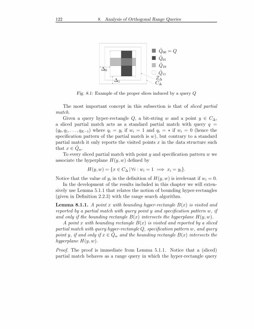
122 8. Analysis of Orthogonal Range Queries
0 1
1 Q00 = Q
Q01
Q10
Q11
∆0
∆1 C∆
Z∆
Fig. 8.1: Example of the proper slices induced by a query Q
The most important concept in this subsection is that of sliced partialmatch.
Given a query hyper-rectangle Q, a bit-string w and a point y ∈ C∆,a sliced partial match acts as a standard partial match with query q =(q0, q1, . . . , qK−1) where qi = yi if wi = 1 and qi = ∗ if wi = 0 (hence thespecification pattern of the partial match is w), but contrary to a standardpartial match it only reports the visited points x in the data structure suchthat x ∈ Qw.
To every sliced partial match with point y and specification pattern w weassociate the hyperplane H(y, w) defined by
H(y, w) = x ∈ C∆ | ∀i : wi = 1 =⇒ xi = yi.Notice that the value of yi in the definition of H(y, w) is irrelevant if wi = 0.
In the development of the results included in this chapter we will exten-sively use Lemma 5.1.1 that relates the notion of bounding hyper-rectangles(given in Definition 2.2.3) with the range search algorithm.
Lemma 8.1.1. A point x with bounding hyper-rectangle B(x) is visited andreported by a partial match with query point y and specification pattern w, ifand only if the bounding rectangle B(x) intersects the hyperplane H(y, w).
A point x with bounding rectangle B(x) is visited and reported by a slicedpartial match with query hyper-rectangle Q, specification pattern w, and querypoint y, if and only if x ∈ Qw and the bounding rectangle B(x) intersects thehyperplane H(y, w).
Proof. The proof is immediate from Lemma 5.1.1. Notice that a (sliced)partial match behaves as a range query in which the hyper-rectangle query

8.1. The Cost of Range Searches 123PSfrag repla ementsQ10Q01 H(v; 10)H(v; 01) H(v; 11) QQQ xxx vvv B(x)B(x)B(x) Q11
Fig. 8.2: Graphical illustration of the proof of Theorem 8.1.2
“degenerates” to the hyperplane H(y, w) (when a coordinate is specified inthe query the corresponding range [ℓi, ui] has identical endpoints; when thecoordinate is not specified we have a corresponding full range). In the case ofsliced partial matches, only those points that also belong to Qw are reported.
8.1.2 The Combinatorial Characterizations
In this subsection we state several relations between the cost R(t) of anorthogonal range search in a K-d tree t and the performance Pw(t, y) of asliced partial match with specification pattern w and query point y in a K-dtree t. The implicit query hyper-rectangle Q is the same for both the rangesearch and the sliced partial match.
Theorem 8.1.2. Given a query Q with corners v0, v1, . . . , v2K−1 and a K-dtree t,
R(t) ≤∑
0≤j<2K
∑
w∈(0+1)K
Pw(t, vj).
Proof. Consider a point x visited by a range search with query Q. Let wbe the index of the proper slice that contains x, i.e., x ∈ Qw. Recall thatsince x is visited by the range search we have B(x) ∩ Q 6= ∅ (Lemma 5.1.1).Therefore, by Lemma 8.1.1, it suffices to show that if B(x) intersects Q thenthere exists at least one corner vj of Q such that the hyperplane H(vj, w)does intersect B(x).If B(x) contains any of the corners of Q then the statement above is clearlytrue: since the hyperplane H(vj, w) contains vj , it must intersect B(x). If

124 8. Analysis of Orthogonal Range Queries
B(x) does not contain any corner of Q, there are two possibilities to consider:either B(x) is entirely within Q, or B(x) intersects one or more faces of Q.If B(x) is totally inside Q then w = 0 . . . 0 and indeed H(vj, 0 . . . 0) = C∆
intersects B(x) for any corner vj . On the other hand, if B(x) intersects oneor more faces of Q but does not contain a corner nor it is contained insideQ then w 6= 11 . . . 1 and Qw must “contact” one of the intersected faces,in the sense that the face is a boundary of Qw. Let f be such face. Now,the hyperplane H(vj, w) contains this face (and hence it intersects B(x)),provided that vj is any corner of the face f (see Fig. 8.2 for a graphicalillustration of this proof when K = 2).
Theorem 8.1.3. Given a query Q with center at z and a K-d tree t,
R(t) ≥∑
w∈(0+1)K
Pw(t, z).
Proof. The statement of the theorem is immediate, once we show that when-ever a point x is reported by a sliced partial match with parameters w and zthen it is also visited by the range search with query Q. Formally, we haveto show that if x ∈ Qw and H(z, w) intersects the bounding rectangle B(x)of x then B(x) also intersects Q. Indeed, if w = 00 . . . 0 then the statementtrivially holds since x ∈ Q. On the other hand, if w 6= 00 . . . 0 then H(z, w)and Qw are disjoint. Since B(x) intersects Qw (x is part of both by hypoth-esis) the only way for B(x) to intersect H(z, w) is to intersect Q too (then,because of Lemma 5.1.1, x must be visited by the range search).
Theorem 8.1.4. Given a query Q with center at z divide C∆ into 2K quad-rants C0, C1, . . . , C2K−1, with z the contact point of the 2K quadrants. LetR(i)(t) denote the number of points of the i−th quadrant visited by a range
search with query Q in the K-d tree t. Similarly, let P(i)w (t, y) denote the
number of points of the i−th quadrant reported by sliced partial match withpattern w and point y in the K-d tree t. Let vi be the unique corner of Qbelonging to the i−th quadrant. Then
R(i)(t) =∑
w∈(0+1)K
P (i)w (t, vi).

8.1. The Cost of Range Searches 125
Proof. For a point x belonging to the i-th quadrant and the proper sliceQw, the intersection of H(vi, w) with B(x) implies the intersection of Q withB(x). On the other hand, if B(x) intersects Q there is at least one corner vsuch that H(v, w) intersects B(x); it is not difficult to see that one of thesecorners must be vi, the unique corner of Q in the i-th quadrant (Fig. 8.2 mayalso help understanding the proof even though quadrants are not depictedthere).
8.1.3 The Cost of Range Search in Relaxed K-d Trees
The theorems of Subsection 8.1.2 show that the analysis of range searchreduces to the analysis of sliced partial matches.
Theorem 8.1.5. Let E [Rn] be the expected cost of a range search with arandom query in a random K-d tree of size n. Let E [Pn,w] be the expectedcost of a sliced partial match with pattern w in a random K-d tree of size n,with respect to a uniformly and independently drawn random query point in[0, 1]K. Then
1
V (Z∆)·∑
w∈(0+1)K
E [Pn,w] ≤ E [Rn] ≤ V (Z∆) ·∑
w∈(0+1)K
E [Pn,w] ,
where V (Z∆) =∏
0≤r<K(1 + ∆r).
Proof. Clearly R(t) =∑
0≤i<2K R(i)(t). Hence,
R(t) =∑
0≤i<2K
∑
w∈(0+1)K
P (i)w (t, vi). (8.1.1)
Given a corner v of a query Q, if v ∈ [0, 1]K let v′ = v, otherwise let v′ bethe point in the boundary of [0, 1]K closest to v (see Fig. 8.3). It is prettyclear that if Q falls partially off the [0, 1]K boundary, the cost of the rangesearch is the same as if we had a range query Q′ where we had chopped thepart of Q that falls outside [0, 1]K. And if we shift a query so that a corner voutside [0, 1]K is aligned to v′ then the corresponding range search will havea cost which is greater or equal to the cost of a range search where we donot perform such a shift. In other words, for any bit-string w, query Q, K-dtree t and quadrant i,
Pw(t, vi) ≤ Pw(t, v′i).

126 8. Analysis of Orthogonal Range Queries
00 1
1PSfrag repla ements QQ vivi v0iv0iFig. 8.3: Shifting queries falling partially off the boundaries.
Hence,
R(t) ≤∑
0≤i<2K
∑
w∈(0+1)K
P (i)w (t, v′
i).
The next step is to take expectations on both sides of the equation above andobserve that, for uniformly distributed centers in Z∆, the probability that vi
falls outside [0, 1]K is(
∏
0≤r<K
(1 + ∆r)
)
− 1.
Then we have
E [Rn] ≤∏
0≤r<K
(1 + ∆r) ·∑
w∈(0+1)K
E
[
P (i)n,w
]
,
where E
[
P(i)n,w
]
is the expected cost of a sliced partial match with respect to
the i-th quadrant and a random uniformly distributed query point in [0, 1]K.Now,
E
[
P (i)n,w
]
= Vol(Ci) · E [Pn,w] ,
where Vol(Ci) is the probability that, given a randomly drawn point z in Z∆,a random data point in [0, 1]K falls in the i-th quadrant defined by z. Since∑
0≤i<2K Vol(Ci) = 1 the upper bound follows.For the lower bound we use Theorem 8.1.3. Taking expectations in bothsides of the inequality of Theorem 8.1.3 and conditioning on the event “thecenter of the query is inside [0, 1]K” the lower bound given in the statementis immediate, as the probability that the center of a random query falls inside[0, 1]K is 1/
∏
0≤r<K(1 + ∆r).

8.1. The Cost of Range Searches 127
Although (8.1.1) gives a precise relationship between the cost of rangesearch and the cost of sliced partial matches, we cannot use it to get resultsabout the variance of Rn or its probability distribution since the costs of thesliced partial matches (the random variables P
(i)n,w) are not independent.
Now we need to analyze the expected cost of sliced partial matches inrandom(ized) relaxed K-d trees. It easily follows from the analysis of theexpected cost of standard partial matches in random relaxed K-d trees [72].Our next theorem gives the expected cost of sliced partial matches in randomrelaxed K-d trees.
Theorem 8.1.6. If w 6= 00 . . . 0 and w 6= 11 . . . 1, the expected cost E [Pn,w]of a sliced partial match in a random relaxed K-d tree of size n w.r.t. arandom query point in [0, 1]K and the pattern w is
E [Pn,w] = Vol(Qw) · β(ρ) · nα(ρ) + O(1),
where ρ = order(w)/K, α ≡ α(x) = (√
9 − 8x − 1)/2, β(x) = Γ(2α +1)/((1− x)(α + 1)α3Γ3(α)), and Vol(Qw) is the probability that a data pointfalls inside the proper slice Qw of a randomly centered query. Furthermore,
E [Pn,00...0] = Vol(Q00...0)·n and E [Pn,11...1] = 2·Vol(Q11...1)·(Hn+1−1), whereHn =
∑
1≤j≤n 1/j = log n + γ + O(1/n) denotes the n-th harmonic number.
Proof. The recurrence for E [Pn,w] is
E [Pn,w] = Vol(Qw) +1
n
∑
0≤k<n
[
ρ ·(
k + 1
n + 1E [Pk,w] +
n − k
n + 1E [Pn−k,w]
)
+ (1 − ρ) · (E [Pk,w] + E [Pn−k,w])]
,
where ρ and Vol(Qw) are defined as in the statement of the theorem.Let yw(x) =
∑
n≥0 E [Pn,w] xn. Then it is easy to show that yw(x) satisfies
xy′′w(x) − 2
2x − 1
1 − xy′
w(x) − 22 − ρ − x
(1 − x)2yw(x) − 2
Vol(Qw)
(1 − x)3= 0, (8.1.2)
and the initial conditions are yw(0) = 0 and y′w(0) = Vol(Qw). The linear
differential equation satisfied by the generating function y(x) of the expectedcost of standard partial matches is almost the same as (8.1.2), except thatthe independent term there is −2/(1−x)3 and y′(0) = 1. It is straightforward

128 8. Analysis of Orthogonal Range Queries
then to show that yw(x) = Vol(Qw) ·y(x). The statement of the theorem nowimmediately follows from the known asymptotic estimates for the expectedcost of standard partial matches in random relaxed K-d trees [72]. Thespecial cases w = 00 . . . 0 (ρ = 0) and w = 11 . . . 1 (ρ = 1) are similarlyhandled; they are even easier, as the first behaves like a full traversal ofthe tree, whereas the second behaves like an exact search in a binary searchtree.
Computing the volumes Vol(Qw) of proper slices turns out to be a difficulttask, both because our model allows queries to fall partially off the boundariesand the data points do not have to be uniformly distributed. On the otherhand, if the ∆i’s are large then the gap between the lower and upper boundsof Theorem 8.1.5 is significant; besides, the random model loses interest asthe “frame” around the data region is also too large. But if the ∆i’s tend to0 as n → ∞ (in other words, the number of reported points does not growlinearly with n) and the data points are uniformly distributed, then we caneasily establish the following corollary.
Corollary 8.1.7. Given a random relaxed K-d tree storing n uniformly andindependently drawn data points in [0, 1]K, the expected cost of a randomrange search of sides ∆0, . . . , ∆K−1 (with ∆i → 0 as n → ∞) with centeruniformly and independently drawn from Z∆, is given by
E [Rn] ∼ ∆0 · · ·∆K−1 · n +∑
1≤j<K
cj · nα(j/K)
+ 2 · (1 − ∆0) · · · (1 − ∆K−1) · log n + O(1),
where
cj = β(j/K) ·∑
w:order(w)=j
(
∏
i:wi=0
∆i
)
·(
∏
i:wi=1
(1 − ∆i)
)
.
Proof. The corollary follows from Theorem 8.1.5 and the asymptotic esti-mates given in Theorem 8.1.6. When ∆i → 0 as n → ∞, we have V (Z∆) → 1;hence the lower and upper bounds in Theorem 8.1.5 match and
E [Rn] ∼∑
w∈(0+1)K
E [Pn,w] .

8.2. Other Multidimensional Data Structures 129
Finally, observe that for the uniform distribution, and provided that the ∆i’sare small enough, we have
Vol(Qw) ∼(
∏
i:wi=0
∆i
)
·(
∏
i:wi=1
(1 − ∆i)
)
.
Notice that the term ∆0 · · ·∆K−1 · n in E [Rn] is the expected number ofreported points and hence the overhead is O(nα(1/K)).
The result above assumes a random model where the queries may fallpartially outside [0, 1]K , but it also gives a very good approximation to theaverage cost of range searches in a random model where the queries mustcompletely fall inside [0, 1]K (again, provided that ∆i → 0 for 0 ≤ i < Kand the centers and data points are uniformly distributed).
8.2 Other Multidimensional Data Structures
It is important to stress that no assumptions were made with respect to theway that discriminants are assigned during the construction of the tree, soall theorems of subsection 8.1.2 and Theorem 8.1.5 apply to standard K-dtrees [4], squarish K-d trees [24], K-d-t trees [22] and other variants. It turnsout that the theorems also apply to quad trees [6] without change.
Furthermore, similar arguments to that of Theorem 8.1.6 are also valid,relating the expected cost of sliced partial matches to the expected cost ofstandard partial matches. In general, when w 6= 00 . . . 0 and w 6= 11 . . . 1 forthe data structures mentioned above we have
E [Pn,w] = βw · Vol(Qw) · nα(ρ) + O(1),
where ρ = order(w)/K, α(x) = 1− x + φ(x) and βw is a constant dependingon w. The expected cost of range search, when ∆i → 0, takes hence the form
E [Rn] = ∆0 · · ·∆K−1 · n +∑
1≤j<K
cj · nα(j/K)
+ 2 · (1 − ∆0) · · · (1 − ∆K−1) · log n + O(1),
(8.2.1)
where cj =∑
w:order(w)=j βw · Vol(Qw),

130 8. Analysis of Orthogonal Range Queries
Different data structures are characterized by different α’s and β’s.The theorems in Section 8.1 also apply to K-d tries, relaxed K-d tries
and quad tries. In order to apply the theorems of Section 8.1, we only needto assume that each internal node “contains” the middle point of the hyper-plane(s) associated to the internal node, to meaningfully define sliced partialmatches in these data structures. The average cost of range searches in thesedigital data structures satisfies (8.2.1), but the βw’s involve a fluctuating pe-riodic term (depending on n) of small amplitude and bounded by a constant.
8.3 A Note on Nearest Neighbor Search
The performance of nearest neighbor search is similar to the overwork inrange search. Given a random K-d tree, the expected cost E [NNn] of anearest neighbor query q uniformly drawn from [0, 1]K is given by the follow-ing expression [14],
E [NNn] = Θ (nρ + log n) ,
where ρ = max0≤s≤K(α(s/K)− 1 + s/K). In the case of standard K-d treesρ ∈ (0.0615, 0.064). More precisely, for K = 2 we have ρ = (
√17 − 4)/2 ≈
0.0615536 and for K = 3 we have ρ ≈ 0.0615254, which is minimal.For relaxed K-d trees ρ ∈ (0.118, 0.125). When K = 2 we have ρ =√
52− 1 ≈ 0.118, which is minimal, whereas for K = 8 we have ρ = 1
8, which
is maximal.
8.4 Experimental Results
We have conducted a series of experiments to validate the theoretical analysisof the previous sections and to explore its limitations, when the input datadoes not fulfill some of the hypotheses of the random model.
Each “sample point” in our experiments consisted of a random relaxed(Tr) and standard (Ts) K-d tree of size n and dimension K, both builtfrom the same sequence of random insertions. Up to Q range searches withrandom queries of given edge lengths were requested in both trees. And thiswas repeated for T pairs (Tr, Ts) of trees of each size and dimension.
The legends of the plots indicate the different parameter values: dimen-sion (K), size (n), number of trees per size (T ), number of queries per tree(Q) and edge lengths (∆). Each plot depicts the empirical expected cost ofrange search against the theoretical predicted value.

8.4. Experimental Results 131
20
30
40
50
0 10000 20000 30000 40000 50000
Fig. 8.4: Relaxed K-d trees (K = 2, n ≤ 50000, T = 300, Q = 100, ∆ =[0.01, 0.01]).
15
20
25
30
0 10000 20000 30000 40000 50000
Fig. 8.5: Relaxed K-d trees (K = 3, n ≤ 50000, T = 300, Q = 100, ∆ =[0.01, 0.01, 0.01]).

132 8. Analysis of Orthogonal Range Queries
12
14
16
18
20
22
24
26
28
0 10000 20000 30000 40000 50000
Fig. 8.6: Relaxed K-d trees (K = 4, n ≤ 50000, T = 300, Q = 100, ∆ =[0.01, 0.01, 0.01, 0.01]).
15
20
25
30
35
40
45
0 10000 20000 30000 40000 50000
Fig. 8.7: Standard K-d trees (K = 2, n ≤ 50000, T = 300, Q = 100, ∆ =[0.01, 0.01]).

8.4. Experimental Results 133
12
14
16
18
20
22
24
26
28
0 10000 20000 30000 40000 50000
Fig. 8.8: Standard K-d trees (K = 3, n ≤ 50000, T = 300, Q = 100, ∆ =[0.01, 0.01, 0.01]).
12
14
16
18
20
22
24
26
0 10000 20000 30000 40000 50000
Fig. 8.9: Standard K-d trees (K = 4, n ≤ 50000, T = 300, Q = 100, ∆ =[0.01, 0.01, 0.01, 0.01]).

134 8. Analysis of Orthogonal Range Queries
0
0.1
0.2
0.3
0.4
0.5
0.6
0.7
0.8
0.1 0.2 0.3 0.4 0.5 0.6 0.7 0.8 0.9 10
0.1
0.2
0.3
0.4
0.5
0.6
0.7
0.8
0.9
1
0 0.1 0.2 0.3 0.4 0.5 0.6 0.7 0.8 0.9 1
Fig. 8.10: Two clustered distributions of n = 1000 points in [0, 1]2 (left: c = 5, σ =[0.1, 0.05]; right: c = 10, σ = [0.05, 0.05]).
The experiments suggest that the variance of the cost of range search ishigh. We conjecture that if E [Rn] = a ·n + b ·nα + o(nα), the variance of Rn
is Θ(n2α).
We have also performed experiments using the same setting as for thefirst set of experiments, but the data points and query centers were drawnfrom a clustered distribution (see for example Fig. 8.10).
In order to generate these clustered distributions, a number of “clusters”is fixed in advance and the centers of the clusters uniformly and indepen-dently generated in [0, 1]K . To generate a data point, a cluster is selected atrandom with identical probability and each coordinate of the point is thengenerated according to a normal law whose mean is the corresponding coor-dinate of the center of the cluster. If the generated data point falls outside[0, 1]K then it is rejected and the procedure repeated.
In our experiments, the number of clusters was c = 10 and the standarddeviations σi of the normal laws were taken all identical to 0.05. The centersof the queries were generated according to the same distribution as the datapoints.
There are two problems for the application of Corollary 8.1.7 to data andrange queries generated according to the model above. First, it is very dif-ficult, if not impossible, to analytically compute the volumes of the properslices. We have prepared a program to compute the approximate valuesof these volumes for given ∆’s, by repeatedly “throwing” queries with thegiven edge lengths and a large number of data points for each query, keep-

8.4. Experimental Results 135
20
40
60
80
100
120
0 10000 20000 30000 40000 50000
20
40
60
80
100
0 10000 20000 30000 40000 50000
Fig. 8.11: Clustered distribution, K = 2, n ≤ 50000, T = 50, Q = 1000,∆ = [0.01, 0.01]. Left: Relaxed K-d trees; right: standard K-d tree.The upper curves in the plots are the theoretical predictions with esti-mated proper slices’ volumes; the middle curves show empirically mea-sured costs; the lower curves are the theoretical predictions with uniformestimates for proper slices’ volumes.

136 8. Analysis of Orthogonal Range Queries
ing frequency counts of the event “point falls in Qw”. For instance, whenK = 2 and ∆ = [0.01, 0.01] we have the estimates Vol(Q00) = 0.000868,Vol(Q01) = 0.022335, Vol(Q10) = 0.019432 and Vol(Q11) = 0.957365, whichare significantly different from the volumes for the given values of ∆ in theuniform distribution.
The second and most important problem is that the data points andquery centers are not independent, so that Corollary 8.1.7 cannot actuallybe applied. However, our experiments show that it still provides reasonableapproximations to the observed data.
The plots for clustered input show the results of the experiments togetherwith: a) the estimates given by Corollary 8.1.7 as if the points where uni-formly distributed; b) the estimates obtained by plugging the “experimental”values of the proper slices’ volumes (see above) into the formula of Corol-lary 8.1.7.
The programs to conduct the experiments where written in C (usingthe GNU gcc-2.8.1 compiler), and run under Solaris 5.7 in a Sun Ultra 5workstation. Awk scripts where used as a front-end to the C program foreasier interaction and for data analysis. The plots were produced with Maple6 and gnuplot.

Part V
CONCLUSIONS AND FUTURE WORK


139
Throughout this work we have presented two different lines of contribu-tions. The first one is the design of point multidimensional data structures(Part III) while the second one is related to the analysis of associative queriesin point multidimensional data structures (Part IV).
Concerning the design of data structures we have introduced two random-ized point multidimensional data structures: randomized relaxed K-d treesand randomized quad trees (Chapters 3 and 4) that have several advantages.Their randomized update algorithms are simple to describe and implement,and for any sequence of interleaved insertions and deletions they always pro-duce random relaxed K-d trees and random quad trees, respectively. Thisimplies that the expected cost of associative queries holds independently ofthe order in which updates are performed. In the case of quad trees theyhave the additional advantage of being defined for any dimension K.
We have thus shown that the use of randomization provides great flex-ibility in the design of point multidimensional data structures and that itguarantees the expected costs of associative queries, with simple search andupdate algorithms.
However, the average case analysis of the split and join operations, whichare in the basis of the given randomized update algorithms, is rather complex(and not given in this work) since it implies the solution of a non-linearsystem of recurrences derived from the interleaved relation existing betweenthem. Since these theoretical results seem difficult to obtain, an experimentalanalysis could provide useful insights. It could also be interesting to test theperformance of both randomized relaxed K-d trees and randomized quadtrees against existing specific benchmarks as well as against real data.
It is worth noting that K-d trees use only one of the possible attributes ofthe records as discriminant at each node while quad trees use all the possibleones. In some sense these two data structures are extreme cases of a possiblefamily of hierarchical multidimensional data structures in which the numberof attributes used as discriminants in each node is variable, going from one(K-d trees) to K (quad trees). We have some evidence in the sense thatformalizing this family of trees and defining randomized update operationson them (which are very similar to the ones for quad trees) can provide ageneral framework for randomized multidimensional data structures. Thisgeneral framework would include also randomized structures such as multi-dimensional skip lists.
We have also introduced in this thesis a new fingering scheme to exploit lo-cality of reference in associative queries on multidimensional data structures.

140
In particular, we have applied these schemes to K-d trees. For the so calledfingered multidimensional trees (Chapter 5) we show that the application ofthis technique results in a significative amelioration of the performance ofhierarchical multidimensional data structures.
A natural extension of this chapter would be to perform the theoreticalanalysis of the overwork of the cost of range queries and nearest neighborqueries. However, it seems a mathematically challenging problem, mostlybecause of backtrack. We think that a first step in this direction are thelemmas (Lemmas 5.1.2, 5.1.3, and 5.1.4) that characterize the given searchalgorithms.
The presented algorithms are straightforwardly applicable to data struc-tures other than K-d trees. For instance, it could be interesting to study theimprovements that this technique might yield for nearest neighbor queries inmetric data structures [15].
Relative to the analysis of associative queries we present the average-caseanalysis of partial match queries in random relaxed K-d trees (Chapter 7)as well as the average-case analysis of orthogonal range queries in severalhierarchical multidimensional data structures such as: K-d trees, K-d tries,quad trees and quad tries (Chapter 8).
The theoretical analysis, developed in this thesis, shows that the algo-rithms for associative queries in randomized relaxed K-d trees have reason-able performance on practical grounds. One of the important results of thisthesis is the connection between orthogonal range queries and partial matchqueries. Even though partial match queries are not as useful in applicationsas range queries and nearest neighbor queries, they are easier to analyzeand their analysis does not involve geometric considerations. Here we haveshown that, for a large family of hierarchical multidimensional data struc-tures, having the analysis of the cost of partial match queries yields at no costthe average performance of orthogonal range and nearest neighbor queries.
As extension of this line of work, we propose the average-case analysisof range queries but under a different query model. The results of orthog-onal range queries presented here depend on a range query model in whichthe range query have given fixed-length sides and the center of the hyper-rectangle is randomly assigned. The obtained results hold for small hyper-rectangles. We suggest another query model in which the hyper-rectanglesare obtained by generating uniformly and independently their corners in[0, 1]K . The obtained range queries will be large with length sizes of 1/3 in

141
average. In the case of random relaxed K-d trees the problem is formallystated in Appendix B.


APPENDIX


A. PLOTS OF FINGERED MULTIDIMENSIONAL TREES

146 A. Plots of Fingered Multidimensional Trees
K = 2
0
0.1
0.2
0.3
0.4
0.5
0.6
0.7
10000 20000 30000 40000 50000
n
K = 3
0
0.1
0.2
0.3
0.4
0.5
10000 20000 30000 40000 50000
n
K = 4
0
0.1
0.2
0.3
0.4
5000 10000 15000 20000 25000 30000 35000
n
K = 5
0
0.05
0.1
0.15
0.2
0.25
0.3
0.35
10000 20000 30000 40000 50000
n
Fig. A.1: Overwork ratios for standard 1-finger K-d trees (thick line) and m-fingerK-d trees (thin line), for δ = 0.25, K = 2 (up left), K = 3 (up right),K = 4 (down left), and K = 5 (down right).
The graphs of Figures A.1, A.2 and A.3 depict τ(1)n and τ
(m)n for standard
1-finger and m-finger K-d trees for δ = 0.25, 0.75 and 2, respectively. Fig-ure A.4 shows the plots of the overwork of standard m-finger K-d trees forseveral values of the locality parameter δ.
The behavior of relaxed 1-finger and m-finger K-d trees for orthogonalrange searches when the queries have variable length sizes is shown in Fig-ures A.5, A.6 and A.7 for δ = 0.25, 0.75 and, 2 respectively. The graphscorresponding to standard 1-finger and m-finger K-d trees are plotted inFigures A.8, A.9 and A.10. It is worth to note that for range queries withvariable length the savings are not as important as for fixed lengths rangequeries. In fact for δ’s greater than 1 there are no savings at all. It is alsoworth noting that the overwork cost is of the same order of growth as thecost of range queries in plain K-d trees.

147
K = 2
0
0.2
0.4
0.6
10000 20000 30000 40000 50000
n
K = 3
0
0.1
0.2
0.3
0.4
0.5
0.6
10000 20000 30000 40000 50000
n
K = 4
0
0.1
0.2
0.3
0.4
5000 10000 15000 20000 25000 30000 35000
n
K = 5
0
0.1
0.2
0.3
0.4
10000 20000 30000 40000 50000
n
Fig. A.2: Overwork ratios for standard 1-finger K-d trees (thick line) and m-fingerK-d trees (thin line), for δ = 0.75, K = 2 (up left), K = 3 (up right),K = 4 (down left), and K = 5 (down right).

148 A. Plots of Fingered Multidimensional Trees
K = 2
0
0.2
0.4
0.6
0.8
10000 20000 30000 40000 50000
n
K = 3
0
0.1
0.2
0.3
0.4
0.5
0.6
0.7
10000 20000 30000 40000 50000
n
K = 4
0
0.1
0.2
0.3
0.4
0.5
0.6
5000 10000 15000 20000 25000 30000 35000
n
K = 5
0
0.1
0.2
0.3
0.4
0.5
10000 20000 30000 40000 50000
n
Fig. A.3: Overwork ratios for standard 1-finger K-d trees (thick line) and m-fingerK-d trees (thin line), for δ = 2, K = 2 (up left), K = 3 (up right), K = 4(down left), and K = 5 (down right).

149
K = 2
5
10
15
20
25
30
35
40
20000 40000 60000 80000
n
K = 3
4
6
8
10
12
14
16
18
10000 20000 30000 40000 50000
n
K = 4
4
6
8
10
5000 10000 15000 20000 25000 30000 35000
n
K = 5
4
5
6
7
8
9
10
10000 20000 30000 40000 50000
n
Fig. A.4: Overwork in standard m-finger K-d trees for several values of the localityparameter δ, K = 2 (up left), K = 3 (up right), K = 4 (down left), andK = 5 (down right).

150 A. Plots of Fingered Multidimensional Trees
K = 2
0
0.1
0.2
0.3
0.4
0.5
0.6
0.7
10000 20000 30000 40000 50000
n
K = 3
0
0.2
0.4
0.6
0.8
10000 20000 30000 40000 50000
n
K = 4
0
0.2
0.4
0.6
0.8
10000 20000 30000 40000 50000
n
K = 5
0
0.2
0.4
0.6
0.8
10000 20000 30000 40000 50000
n
Fig. A.5: Overwork ratios for relaxed 1-finger K-d trees (thick line) and m-fingerK-d trees (thin line), for δ = 0.25, and ∆ = K
√
1/n, K = 2 (up left),K = 3 (up right), K = 4 (down left), and K = 5 (down right).

151
K = 2
0
0.1
0.2
0.3
0.4
0.5
0.6
0.7
10000 20000 30000 40000 50000
n
K = 3
0
0.2
0.4
0.6
0.8
10000 20000 30000 40000 50000
n
K = 4
0
0.2
0.4
0.6
0.8
10000 20000 30000 40000 50000
n
K = 5
0
0.2
0.4
0.6
0.8
1
10000 20000 30000 40000 50000
n
Fig. A.6: Overwork ratios for relaxed 1-finger K-d trees (thick line) and m-fingerK-d trees (thin line), for δ = 0.75, and ∆ = K
√
1/n, K = 2 (up left),K = 3 (up right), K = 4 (down left), and K = 5 (down right).

152 A. Plots of Fingered Multidimensional Trees
K = 2
0
0.2
0.4
0.6
0.8
10000 20000 30000 40000 50000
n
K = 3
0
0.2
0.4
0.6
0.8
10000 20000 30000 40000 50000
n
K = 4
0
0.2
0.4
0.6
0.8
1
10000 20000 30000 40000 50000
n
K = 5
0
0.2
0.4
0.6
0.8
1
10000 20000 30000 40000 50000
n
Fig. A.7: Overwork ratios for relaxed 1-finger K-d trees (thick line) and m-fingerK-d trees (thin line), for δ = 2, and ∆ = K
√
1/n, K = 2 (up left), K = 3(up right), K = 4 (down left), and K = 5 (down right).

153
K = 2
0
0.1
0.2
0.3
0.4
0.5
0.6
10000 20000 30000 40000 50000
n
K = 3
0
0.2
0.4
0.6
0.8
10000 20000 30000 40000 50000
n
K = 4
0
0.2
0.4
0.6
0.8
10000 20000 30000 40000 50000
n
K = 5
0
0.2
0.4
0.6
0.8
10000 20000 30000 40000 50000
n
Fig. A.8: Overwork ratios for standard 1-finger K-d trees (thick line) and m-fingerK-d trees (thin line), for δ = 0.25, and ∆ = K
√
1/n, K = 2 (up left),K = 3 (up right), K = 4 (down left), and K = 5 (down right).

154 A. Plots of Fingered Multidimensional Trees
K = 2
0
0.1
0.2
0.3
0.4
0.5
0.6
0.7
10000 20000 30000 40000 50000
n
K = 3
0
0.2
0.4
0.6
0.8
10000 20000 30000 40000 50000
n
K = 4
0
0.2
0.4
0.6
0.8
10000 20000 30000 40000 50000
n
K = 5
0
0.2
0.4
0.6
0.8
1
10000 20000 30000 40000 50000
n
Fig. A.9: Overwork ratios for standard 1-finger K-d trees (thick line) and m-fingerK-d trees (thin line), for δ = 0.75, and ∆ = K
√
1/n, K = 2 (up left),K = 3 (up right), K = 4 (down left), and K = 5 (down right).

155
K = 2
0
0.2
0.4
0.6
0.8
10000 20000 30000 40000 50000
n
K = 3
0
0.2
0.4
0.6
0.8
10000 20000 30000 40000 50000
n
K = 4
0
0.2
0.4
0.6
0.8
1
10000 20000 30000 40000 50000
n
K = 5
0
0.2
0.4
0.6
0.8
1
10000 20000 30000 40000 50000
n
Fig. A.10: Overwork ratios for standard 1-finger K-d trees (thick line) and m-finger K-d trees (thin line), for δ = 2, and ∆ = K
√
1/n, K = 2 (up left),K = 3 (up right), K = 4 (down left), and K = 5 (down right).

156 A. Plots of Fingered Multidimensional Trees
K = 2
0.82
0.84
0.86
0.88
0.9
20000 40000 60000 80000 100000
n
K = 3
0.92
0.925
0.93
0.935
0.94
20000 40000 60000 80000 100000
n
K = 4
0.915
0.92
0.925
0.93
0.935
0.94
0.945
0.95
20000 40000 60000 80000 100000
n
K = 5
0.912
0.914
0.916
0.918
0.92
0.922
0.924
0.926
0.928
0.93
20000 40000 60000 80000 100000
n
Fig. A.11: Nearest neighbor queries in standard 1-finger K-d trees for δ = 0.005,K = 2 (up left), K = 3 (up right), K = 4 (down left), and K = 5 (down
right).

157
K = 2
0.77
0.78
0.79
0.8
0.81
0.82
0.83
0.84
0 10000 20000 30000 40000 50000
n
K = 3
0.93
0.94
0.95
0.96
0.97
0 10000 20000 30000 40000 50000
n
K = 4
0.94
0.95
0.96
0.97
0.98
0 10000 20000 30000 40000 50000
n
K = 5
0.94
0.95
0.96
0.97
0 10000 20000 30000 40000 50000
n
Fig. A.12: Nearest neighbor queries in standard 1-finger K-d trees for δ =0.25 K
√
1/n, K = 2 (up left), K = 3 (up right), K = 4 (down left),and K = 5 (down right).


B. ANALYSIS OF ORTHOGONAL RANGE QUERIESWITH RANDOM CORNERS

160 B. Analysis of Orthogonal Range Queries with Random Corners
Let F = x(0), . . . , x(n), n ≥ 0, be the given file (set of K-dimensionalpoints). Each x ∈ F is thus a K-tuple x = (x1, x2, . . . , xK−1), where each xi
belongs to some totally ordered domain Di. Hence, x ∈ D = D0×· · ·×DK−1.Let −∞ and +∞ denote special values such that for any v ∈ Di, −∞ < vand v < +∞, according to the total order defined in Di, and let Di =Di ∪ −∞, +∞, and D = D0 × · · · × DK−1.
Then a range query is a hyper-rectangle Q ∈ D×D ∼ (D0×D0)× (D1×D1) × · · · (DK−1 × DK−1).
Let Q = (ℓ0, u0)×(ℓ1, u1)×· · ·×(ℓK−1, uK−1), with −∞ ≤ li ≤ ui ≤ +∞,for 0 ≤ i < K. If li = −∞ and ui = +∞ we say that the i-th coordinateof H is unspecified. If li = −∞ or ui = +∞, but not both, we say that thei-th coordinate is half-specified. If −∞ < li ≤ ui < +∞, the coordinate isfully-specified.
Let Ru,h(n) denote the expected cost (measured as number of visitednodes) in a random range query with u unspecified coordinates and h half-specified coordinates, 0 ≤ u ≤ K, 0 ≤ h ≤ K, u + h ≤ K, in a randomrelaxed K-d tree of size n. Trivially, Ru,h(n) = n if n ≤ 1, for all u and h.Furthermore, for any n ≥ 0,
RK,0(n) = n,
since range search reduces to a pre-order traversal of the whole tree when alldimensions are unspecified.
Now, assume u < K and n > 0. The random relaxed K-d tree Tn has aleft subtree L and a right subtree of sizes k and n − 1 − k with probability1/n, for 0 ≤ k < n. If the discriminant of the root node is one of the un-specified coordinates, which happens with probability u/K, then the searchcontinues recursively in both subtrees. On the other hand, if the discrim-inant, say j, is a half-specified coordinate (with probability h/K) then wehave two possibilities: either the value xj of the element stored in the rootis inside the half-specified range or it is not. By symmetry, we might onlyconsider half-specified ranges such that uj = +∞. The first case occurs thenwith probability (k + 1)/(n + 1) and we have to continue with the searchin both subtrees; however, the range search in the right subtree will be nowunspecified with respect to the j-th coordinate. Therefore, we will have aterm of the type
k + 1
n + 1(Ru,h(k) + Ru+1,h−1(n − 1 − k)) .

161
The second case (xj fails off the range) occurs with probability (n−k)/(n+1);in this case, we only make one recursive call in the right subtree.
Last but not least, the discriminant can be fully-specified (with proba-bility 1 − (u + h)/K) and we can have three cases: the range is to the leftof the root’s element along the j-th coordinate (uj < xj), the range is tothe right (xj ≤ ℓj) or the range covers the element (ℓj < xj ≤ uj). Theseevents happen with probabilities (k + 1)2/(n + 1)2, (n − k)2/(n + 1)2 and2(k + 1)(n − k)/(n + 1)2, respectively. In the first case, we explore only theleft subtree, in the second case we explore only the right subtree, and finally,in the third case we explore both subtrees, but now the j-th coordinate ishalf-specified in the two recursive calls.
Collecting everything the recurrence when n > 0 is as follows.
Ru,h(n) = 1 + 1n
∑
0≤k<n
[
uK
(Ru,h(k) + Ru,h(n − 1 − k))
+ hK
(
n−kn+1
Ru,h(n − 1 − k) + k+1n+1
(Ru,h(k) + Ru+1,h−1(n − 1 − k))
)
+(
1 − u+hK
)
(
(
k+1n+1
)2Ru,h(k) +
(
n−kn+1
)2Ru,h(n − 1 − k)
+2 (k+1)(n−k)(n+1)2
(Ru,h+1(k) + Ru,h+1(n − 1 − k))
)]
.
By obvious symmetries the recurrence above can be simplified to,
Ru,h(n) = 1 + 2unK
∑
0≤k<n Ru,h(k)
+ 2hnK
∑
0≤k<nk+1n+1
Ru,h(k)
+ hnK
∑
0≤k<nn−kn+1
Ru+1,h−1(k)
+2(K−(u+h))nK
∑
0≤k<n
(
k+1n+1
)2Ru,h(k)
+4(K−(u+h))nK
∑
0≤k<n(k+1)(n−k)
(n+1)2Ru,h+1(k).
Notice that the recurrence is valid even if u = K, since only the first twoterms are then non-zero.

162 B. Analysis of Orthogonal Range Queries with Random Corners
For example, take K = 2. We are interested in R0,0(n). Using therecurrence above we readily see that we need the value of R0,1(n). To solvethe recurrence for R0,1(n) we will have to solve before the recurrences forR1,0(n) and R0,2(n) and so forth. In general, Ru,h(n) depends on Ru+1,h−1(k),Ru,h+1(k) and Ru,h(k − 1) with 0 ≤ k < n. The graphs of interrelationsamong the Ru,h’s is acyclic; about K2/2 recurrences need to be solved toobtain R0,0(n) (which is actually the sought answer).
We have the solutions for the recurrences of the form RK−i,i and R0,i fori = 0, . . . , K but we have not been able to go any further.

BIBLIOGRAPHY
[1] C. R. Aragon and R. G. Seidel. Randomized search trees. In Pro-ceedings of the 30th IEE Symposium on Foundations of Computer Sci-ence(FOCS), pages 540–545, 1989.
[2] R. Bayer. The universal B-tree for multidimensional in-dexing. Technical Report TUM–I9637, Technische Univer-sitat Munchen, Munich, Germany, 1996. Available fromhttp://wwwbib.informatik.tu-muenchen.de/infberichte/1996/.
[3] N. Beckmann, H. P. Kriegel, R. Schneider, and B. Seeger. The R∗-tree:an efficient and robust access method for points and rectangles. InProceedings of the ACM SIGMOD International Conference on Man-agement of Data, pages 322–331, 1990.
[4] J. L. Bentley. Multidimensional binary search trees used for associativeretrieval. Communications of the ACM, 18(9):509–517, 1975.
[5] J. L. Bentley. Decomposable searching problems. Information Process-ing Letters, 8(5):133–136, 1979.
[6] J. L. Bentley and R. A. Finkel. Quad trees: A data structure forretrieval on composites keys. Acta Informatica, 4:1–9, 1974.
[7] J. L. Bentley, D. F. Stanat, and E. H. Williams. The complexity offinding fixed-radius near neighbors. Information Processing Letters,6(6):209–212, 1977.
[8] J.L. Bentley and J. H. Friedman. Data structures for range searching.ACM Computing Surveys, 11(4):397–409, 1979.
[9] S. Berchtold, D. Keim, and H. P. Kriegel. The X-tree: an index struc-ture for multidimensional data. In Proceedings of the 22nd. Interna-

164 Bibliography
tional Conference on Very Large Databases, (Bombay), pages 28–39,1996.
[10] H. Blanken, A. Ijbema, P. Meek, and B. van den Akker. The generalizedgrid file: Description and performance aspects. In Proceedings of theSixth IEEE Internatinal Conference on Data Engineering, pages 380–388, 1990.
[11] A. Borodin and R. El-Yaniv. On line Computation and CompetitiveAnalysis. Cambridge University Press, 1998.
[12] M. R. Brown and R. E. Tarjan. Design and analysis of a data structurefor representing sorted lists. SIAM Journal on Computing, 9(3):594–614, 1980.
[13] W. A. Burkhard. Hashing and trie algorithms for partial match re-trieval. ACM Transactions on Database Systems, 1(2):175–187, 1976.
[14] P. Chanzy, L. Devroye, and C. Zamora-Cura. Analysis of range searchfor random k-d trees. Acta Informatica, 37:355–383, 2001.
[15] E. Chavez, G. Navarro, R. Baeza-Yates, and J. L. Marroquın. Searchingin metric spaces. ACM Computing Surveys, 33(3):273–321, 2001.
[16] H. H. Chern and H. K. Hwang. An asymptotic theory for Cauchy-Eulerdifferential equations with applications to the analysis of algorithms.Journal of Algorithms, 44(1):177–225, 2002.
[17] H. H. Chern and H. K. Hwang. Partial match queries in random k-dtrees, 2003. Submitted for publication.
[18] H. H. Chern and H. K. Hwang. Partial match queries in random quadtrees. SIAM Journal on Computing, 32(4):904–915, 2003.
[19] D. Comer. The ubiquitous B-tree. ACM Computing Surveys,11(2):121–137, 1979.
[20] The Unicode Consortium. The Unicode Standard Version 2.0, 2d. Edi-tion. Addison–Wesley, 1996.
[21] J. Culberson. The effect of updates in binary search trees. In ACMSymp. on the Theory of Computing (STOC’85), pages 205–212, 1985.

Bibliography 165
[22] W. Cunto, G. Lau, and Ph. Flajolet. Analysis of KDT -trees: KD-trees improved by local reorganisations. In F. Dehne, J. R. Sack,and N. Santoro, editors, Workshop on Algorithms and Data Structures(WADS’89), volume 382 of LNCS, pages 24–38. Springer–Verlag, 1989.
[23] L. Devroye. Branching processes in the analysis of the height of trees.Acta Informatica, 24:277–298, 1987.
[24] L. Devroye, J. Jabbour, and C. Zamora-Cura. Squarish k-d trees. SIAMJournal on Computing, 30:1678–1700, 2000.
[25] L. Devroye and L. Laforest. An analysis of random d-dimensionalquadtrees. SIAM Journal on Computing, 19(5):821–832, 1990.
[26] A. Duch. Randomized insertion and deletion in point quad trees.In Int. Symposium on Algorithms and Computation (ISAAC), LNCS.Springer–Verlag, 2004. Accepted for publication.
[27] A. Duch, V. Estivill-Castro, and C. Martınez. Randomized K-dimensional binary search trees. In K.-Y. Chwa and O. H. Ibarra,editors, Int. Symposium on Algorithms and Computation (ISAAC’98),volume 1533 of LNCS, pages 199–208. Springer-Verlag, 1998.
[28] A. Duch, V. Estivill-Castro, and C. Martınez. Randomized K-dimensional binary search trees. Technical Report LSI–98–48–R, LSI-UPC, 1998.
[29] A. Duch and C. Martınez. On the average performance of orthogonalrange search in multidimensional data structures. In P. Widmayer,F. Triguero, R. Morales, R. Henessy, S. Eidenbenz, and R. Conejo, edi-tors, Proc. of the 29th. Int. Col. on Automata, Languages and Program-ming (ICALP), volume 2380 of LNCS, pages 514–524. Springer–Verlag,2002.
[30] A. Duch and C. Martınez. On the average performance of orthogonalrange search in multidimensional data structures. Journal of Algo-rithms, 44(1):226–245, 2002.
[31] A. Duch and C. Martınez. Fingered multidimensional search trees.In C. C. Ribeiro and S. L. Martins, editors, Proc. of the Third Inter-national Workshop on Experimental and Efficient Algorithms (WEA),volume 3059 of LNCS, pages 228–242. Springer–Verlag, 2004.

166 Bibliography
[32] J. L. Eppinger. An empirical study of insertion and deletion in binarysearch trees. Communications of the ACM, 26(9):663–669, 1983.
[33] G. Evangelidis, D. Lomet, and B. Salzberg. The hBπ-tree: a mod-ified hB-tree supporting concurrency, recovery and node consolida-tion. In Proceedings of the 21st International Conference on Very LargeDatabases, pages 551–561, 1996.
[34] R. A. Finkel and J. L. Bentley. Quad trees: a data structure for retrievalon composite key. Acta Informatica, 4(1):1–9, 1974.
[35] Ph. Flajolet, G. Gonnet, C. Puech, and J. M. Robson. Analytic varia-tions on quad trees. Algorithmica, 10:473–500, 1993.
[36] Ph. Flajolet and T. Lafforgue. Search costs in quad trees and singu-larity perturbation analysis. Discrete and Computational Geometry,12(4):151–175, 1993.
[37] Ph. Flajolet and A. Odlyzco. Singularity analysis of generating func-tions. SIAM Journal of Discrete Mathematics, 3(1):216–240, 1990.
[38] Ph. Flajolet and C. Puech. Partial match retrieval of multidimensionaldata. Journal of the ACM, 33(2):371–407, 1986.
[39] M. Freeston. A general solution of the n-dimensional B-tree prob-lem. In Proceedings of the ACM SIGMOD International Conferenceon Management of Data, pages 80–91, 1995.
[40] J. H. Friedman, J. L. Bentley, and R. A. Finkel. An algorithm forfinding best matches in logarithmic expected time. ACM Transactionson Mathematical Software, 3(3):209–226, 1977.
[41] M. Friedman, F. Baskett, and L. J. Shustek. An algorithm for findingnearest neighbors. IEEE Transactions on Computing, C–24(10):1000–1006, 1975.
[42] H. Fuchs, Z. Kedem, and B. Naylor. On visible surface generation bya priori tree structures. Computer Graphics, 14(3), 1980.
[43] V. Gaede and O. Gunther. Multidimensional access methods. ACMComputing Surveys, 30(2):170–231, 1998.

Bibliography 167
[44] R. L. Graham, D. E. Knuth, and O. Patashnik. Concrete Mathematics,2nd edition. Addison–Wesley, 1994.
[45] L. J. Guibas, E. M. McCreight, M. F. Plass, and J. R. Roberts. A newrepresentation for linear lists. In Symp. on the Theory of Computing(STOC), 1977.
[46] O. Gunter. Efficient Structures for Efficient Data Management, volume337 of LNCS. Springer–Verlag, 1988.
[47] O. Gunter. Evaluation of spatial access methods with oversize shelves.In G. Gambosi, M. Scholl, and H. Six, editors, Geographic DatabaseManagement Systems, pages 177–193. Springer–Verlag, 1991.
[48] A. Guttman. R-trees: a dynamic index structure for spatial searching.Proc. of the ACM–SIGMOD Annual Meeting, 14(2):47–54, 1984.
[49] A. Henrich and J. Moller. Extending spatial access structures to sup-port additional standard attributes. In M. J. Egenhofer and J. R.Herring, editors, Proceedings of the 4th Int. Symp. on Advances in Spa-tial Data Bases, volume 951 of LNCS, pages 132–151. Springer–Verlag,1995.
[50] A. Henrich, H. W. Six, and P. Widmayer. The LSD tree: Spatial accessto multidimensional point and non-point objects. In Proceedings of theFifteenth International Conference on Very Large Data Bases, pages45–53, 1989.
[51] P. Henrici. Applied and Computational Complex Analysis, volume 1.Wiley-Interscience, 1974.
[52] P. Henrici. Applied and Computational Complex Analysis, volume 2.Wiley-Interscience, 1977.
[53] K. Hinrichs. Implementation of the grid file: design, concepts andexperience. BIT, 25:569–592, 1985.
[54] A. Hutflesz, H. W. Six, and P. Widmayer. Twin grid files: Spaceoptimizing access schemes. In Proceedings of the ACM SIGMOD In-ternational Conference on Management of Data, pages 183–190, 1988.

168 Bibliography
[55] H. V. Jagadish. Spatial search with polyhedra. In Proceedings of theFifth IEEE International Conference on Data Engineering, pages 311–319, 1990.
[56] I. Kamel and C. Faloutsos. Parallel R-trees. In Proceedings of the ACMSIGMOD Conference on Management of Data, pages 195–204, 1992.
[57] I. Kamel and C. Faloutsos. Hilbert R-trees: An improved R-tree usingfractals. In Proceedings of the Twentieth International Conference onVery Large Data Bases, pages 500–509, 1994.
[58] J. S. Karlsson and M. L. Kersten. Omega-storage: A self organizingmulti-attibute storage technique for very large main memories. Reportof the Centrum voor Wiskunde en Informatica, 1999.
[59] P. Kirschenhofer and H. Prodinger. Multidimensional digital searchingin alternative data structures. Random Structures and Algorithms,5(1):123–134, 1994.
[60] D. E. Knuth. The art of computer programming, vol. 3: sorting andsearching, 2nd. edition. Addison–Wesley, Reading, Mass., 1999.
[61] H. P. Krieger and B. Seeger. Multidimensional order preserving linearhashing with partial expansions. In Proceedings of the InternationalConference on Database Theory, volume 243 of LNCS. Springer–Verlag,1986.
[62] H. P. Krieger and B. Seeger. Multidimensional quantile hashing isvery efficient for non-uniform record distributions. In Proceedings ofthe Third IEEE International Conference on Data Engineering, pages10–17, 1987.
[63] H. P. Krieger and B. Seeger. PLOP-hashing: a grid file without direc-tory. In Proceedings of the Fourth IEEE International Conference onData Engineering, pages 369–376, 1988.
[64] H. P. Krieger and B. Seeger. Multi dimensional quantile hashing is veryefficient for non-uniform distributions. Information Science, 48:99–117,1989.

Bibliography 169
[65] A. Kumar. G-tree: A new data structure for organizing multidimen-sional data. IEEE Trans. Knowl. Data Eng., 6(2):341–347, 1994.
[66] D. T. Lee and C. K. Wong. Worst-case analysis for region and partialregion searches in multidimensional binary search trees and quad-trees.Acta Informatica, 9(1):23–29, 1977.
[67] R. C. T. Lee, T. H. Chin, and S. C. Chang. Application to principalcomponent analysis to multi–key searching. IEEE Transactions onSoftware Eng., SE-2(3):185–193, 1976.
[68] K. I. Lin, H. Jagadish, and C. Faloutsos. The TV -tree: An indexstructure for high-dimensional data. VLDB J., 3(4):517–543, 1994.
[69] D. B. Lomet and B. Salzberg. The hB-tree: A robust multi attributesearch structure. In Proceedings of the Fifth IEEE International Con-ference on Data Engineering, pages 296–304, 1989.
[70] H. M. Mahmoud. Evolution of Random Search Trees. Wiley–Interscience Series. John Wiley and Sons, 1992.
[71] C. Martınez, A. Panholzer, and H. Prodinger. On the number of de-scendants and ascendants in random search trees. Electronic Journalon Combinatorics, 5(1):181–204, 1998.
[72] C. Martınez, A. Panholzer, and H. Prodinger. Partial match queries inrelaxed multidimensional search trees. Algorithmica, 29(1–2):181–204,2001.
[73] C. Martınez and S. Roura. Randomized binary search trees. Journalof the ACM, 45(2):288–323, 1998.
[74] T. Matsuyama, L. Hao, and M. Nagao. A file organization for geo-graphic information systems based on spatial proximity. J. Comput.Vis. Graph. Image Process., 26(3):303–318, 1984.
[75] R. Motwani and P. Raghavan. Randomized Algorithms. CambridgeUniversity Press, 1995.
[76] K. Mulmuley. Randomized multidimensional search trees: further re-sults in dynamic sampling. Proceedings of the 32nd IEEE Symposiumon Foundations of Computer Science (FOCS), pages 216–227, 1991.

170 Bibliography
[77] K. Mulmuley. Randomized multidimensional search trees: lazy balanc-ing and dynamic shuffling. Proceedings of the 32nd IEEE Symposiumon Foundations of Computer Science (FOCS), pages 180–196, 1991.
[78] R. Neininger. Limit Laws for Random Recursive Structures and Algo-rithms. Dissertation, Universitat Freiburg i. Br., 1999.
[79] R. Neininger. Asymptotic distributions for partial match queries in K-dtrees. Random Structures and Algorithms, 17(3–4):403–4027, 2000.
[80] J. Nievergelt, H. Hinterberger, and K. C. Sevcik. The grid file: Anadaptable symmetric multikey file structure. ACM Transactions onDatabase Systems, 1(9):38–71, 1984.
[81] Y. Ohsawa and M. Sakauchi. BD-tree: A new n-dimensional datastructure with efficient dynamic characteristics. In Proceedings of theNinth World Computer Congress, IFIP, pages 539–544, 1983.
[82] Y. Ohsawa and M. Sakauchi. A new tree type data structure with ho-mogenous node suitable for a very large spatial database. In Proceed-ings of the Sixth IEEE International Conference on Data Engineering,pages 296–303, 1990.
[83] B. C. Ooi, K. J. McDonell, and R. Sacks-Davis. Spatial kd-tree: Anindexing mechanism for spatial data bases. In Proceedings of the IEEEComputer Software and Applications Conference, pages 433–438, 1987.
[84] P. Oosterom. Reactive Data Structures for Geographic InformationSystems. PhD Thesis, University of Leiden, The Netherlands., 1990.
[85] J. Orenstein and T. H. Merrett. A class of data structures for associa-tive searching. In Proceedings of the Third ACM SIGACT-SIGMODSymposium on Principles of Data base Systems, pages 181–190, 1984.
[86] M. H. Overmars and J. van Leeuwen. Dynamic multi-dimensional datastructures based on quad- and k-d-trees. Acta Informatica, 17(3):267–285, 1982.
[87] W. Pugh. Skip lists: A probabilistic alternative to balance trees. Com-munications of the ACM, 33(6):668–676, 1990.

Bibliography 171
[88] M. Regnier. Analysis of the grid file algorithms. BIT, 25(2):335–357,1985.
[89] R. L. Rivest. Partial-match retrieval algorithms. SIAM Journal onComputing, 5(1):19–50, 1976.
[90] J. T. Robinson. The KDB-tree: A search structure for large multidi-mensional dynamic indexes. Proceedings of the ACM SIGMOD Inter-national Conference on Management of Data, pages 10–18, 1981.
[91] N. Roussopoulos and D. Leifker. Direct spatial search on pictorialdatabases using packed R-trees. Proceedings of the ACM SIGMODInternational Conference on Management of Data, pages 17–31, 1985.
[92] H. Sagan. Space Filling Curves. Springer–Verlag, 1994.
[93] H. Samet. Deletion in two-dimensional quad-trees. Communicationsof the ACM, 23(12):703–710, 1980.
[94] H. Samet. Applications of Spatial Data Structures. Addison–Wesley,1990.
[95] H. Samet. The Design and Analysis of Spatial Data Structures.Addison–Wesley, 1990.
[96] R. Schneider and H. P. Kriegel. The TR∗-tree: A new representationof polygonal objects supporting spatial queries and operations. In Pro-ceedings of the Seventh Workshop on Computational Geometry, volume553 of LNCS, pages 249–264. Springer–Verlag, 1992.
[97] B. Seeger and H. P. Kriegel. Techniques for design and implementationof spatial access methods. In Proceedings of the Fourteenth Interna-tional Conference on Very Large Databases, pages 360–371, 1988.
[98] T. Sellis, N. Roussopoulos, and C. Faloutsos. The R+-tree: A dy-namic index for multi-dimensional objects. In Proceedings of the Thir-teenth International Conference on Very Large Databases, pages 507–518, 1987.
[99] Y.V. Silva-Filho. Average case analysis of region search in balancedk-d trees. Information Processing Letters, 8(5):219–223, 1979.

172 Bibliography
[100] D. Sleator and R. E. Tarjan. Amortized efficiency of list update andpaging rules. Communications of the ACM, 28(2):202–208, 1985.
[101] R. Sproull. Refinements to nearest neighbor searching in k-dimensionaltrees. Algorithmica, 6(4):579–589, 1991.
[102] M. Tamminen. The extendible cell method for closest point problems.BIT, 22:27–41, 1982.
[103] M. J. van Kreveld and M. H. Overmars. Divided k-d trees. Algorith-mica, 6(6):840–858, 1991.
[104] J. S. Vitter and Ph. Flajolet. Average-case analysis of algorithmsand data structures. In J. van Leewen, editor, Handbook of Theoret-ical Computer Science, volume A, chapter 9. North–Holland, 1990.