desi g n, simula tio n , a nd st abili ty of...
TRANSCRIPT

DESIGN, SIMULATION, AND STABILITY OF A
HEXAPEDAL RUNNING ROBOT
a dissertation
submitted to the department of mechanical engineering
and the committee on graduate studies
of stanford university
in partial fulfillment of the requirements
for the degree of
doctor of philosophy
Jonathan E. Clark
August 2004

c! Copyright by Jonathan E. Clark 2004
All Rights Reserved
ii
I certify that I have read this dissertation and that, in
my opinion, it is fully adequate in scope and quality as a
dissertation for the degree of Doctor of Philosophy.
Mark R. Cutkosky(Principal Adviser)
I certify that I have read this dissertation and that, in
my opinion, it is fully adequate in scope and quality as a
dissertation for the degree of Doctor of Philosophy.
Scott L. Delp
I certify that I have read this dissertation and that, in
my opinion, it is fully adequate in scope and quality as a
dissertation for the degree of Doctor of Philosophy.
Kenneth J. Waldron
Approved for the University Committee on Graduate
Studies.
iii

Abstract
Animals are the current gold standard of locomotion ability. Their ability to nav-
igate rough terrain is unmatched by their man-made counterparts. Recent studies
by biologists have begun to demonstrate some of the principles behind their remark-
able capabilities. In particular, studies of cockroaches have shown that they use a
feed-forward motor actuation pattern that is virtually unchanged, even when running
over very rough terrain. It appears that their considerable structural compliance
contributes significantly to their stability when running. Their sprawled posture and
tuned impedance in their musculoskeletal system enable an instantaneous or preflex
response to disturbances. This allows for rapid response to the large perturbations
experienced when interacting with irregular terrain.
Consideration of these principles has led to the design of the Sprawl family of
robots, which features one active thruster and one entirely passive rotary joint on
each leg. Without these spring elements the robots would not be able to run. With
them, they can easily overcome hip-height obstacles without any alteration of their
open-loop controller. The robots function as tuned oscillating systems and small
changes in their physical parameters (e.g. leg sti!ness and damping) can produce
large changes in their speed and stability.
Simple conceptual models of hopping have been used to analyze the e!ects of
modifying the open-loop control system on system performance. These simple one-
legged models have proven e!ective in helping to tune the actuation dynamics of the
robot, but their simplicity precludes their use in tuning the sprawled self-stabilizing
posture of the robot.
This thesis describes the development, calibration, and analysis of a three-dimensional
iv

dynamic simulation of the Sprawl robots. This simulation was developed as a de-
sign tool to investigate the e!ects of parameter variation, and to gain understanding
about how to tune the leg configuration and hip impedance which constitute the
self-stabilizing posture of the robot.
The simulation is used to characterize the sensitivity of the system’s performance
to changes in the robots’ physical parameters. The key parameters that influence
speed and stability are identified, and their e!ects and the nature of their coupling
are investigated. In particular, the coupling between actuation and environmental
parameters is evaluated. The simulation results suggest that for changing slopes and
surface friction altering the leg configuration and (to a lesser degree) the actuation
frequency of the robot may dramatically increase performance.
While speed is easy to measure, no universal metric for running stability exists.
This thesis discusses four distinct steady-state measures of stability that are applicable
to a simulated running robot. The e!ect of modifying the posture of the robot on
stability is investigated for each of these measures. These results delineate the nature
of the trade o! between speed and stability, and indicate advantageous design points
to maximize both.
As a demonstration of its utility as a design tool, the simulation is used to tune the
performance of one of the Sprawl robots. The mass distribution, hip impedance, and
leg postures of the model are adjusted to improve speed while preserving stability.
The resulting design was implemented on the physical robot. The simulation-based
design was compared to the empirically tuned robot settings and the modified design
resulted in a two-fold increase of the robot’s speed.
v

Dedicated to . . .
vi

Contents
Abstract iv
vi
1 Introduction 1
1.1 Motivation . . . . . . . . . . . . . . . . . . . . . . . . . . . . . . . . . 2
1.2 Challenges . . . . . . . . . . . . . . . . . . . . . . . . . . . . . . . . . 2
1.3 Contributions . . . . . . . . . . . . . . . . . . . . . . . . . . . . . . . 3
1.4 Thesis Overview . . . . . . . . . . . . . . . . . . . . . . . . . . . . . . 4
2 Previous Work 6
2.1 Walking Robots . . . . . . . . . . . . . . . . . . . . . . . . . . . . . . 7
2.1.1 Early Walkers . . . . . . . . . . . . . . . . . . . . . . . . . . . 7
2.1.2 Centralized Controller . . . . . . . . . . . . . . . . . . . . . . 8
2.1.3 Gait Generation Via Distributed Control . . . . . . . . . . . . 9
2.1.4 Static Stability Margins . . . . . . . . . . . . . . . . . . . . . 10
2.1.5 Dynamic Stability Margins . . . . . . . . . . . . . . . . . . . . 12
2.1.6 Bipedal Walking Stability . . . . . . . . . . . . . . . . . . . . 13
2.1.7 Walking Constraints . . . . . . . . . . . . . . . . . . . . . . . 15
2.2 Dynamic Locomotion . . . . . . . . . . . . . . . . . . . . . . . . . . . 16
2.2.1 Hopping Robots . . . . . . . . . . . . . . . . . . . . . . . . . . 16
2.2.2 Passive Dynamic Bipeds . . . . . . . . . . . . . . . . . . . . . 17
2.2.3 Stability Analysis for Simple Dynamic Systems . . . . . . . . 18
2.3 Multi-legged Runners . . . . . . . . . . . . . . . . . . . . . . . . . . . 19
vii

2.3.1 Mammalian Runners . . . . . . . . . . . . . . . . . . . . . . . 19
2.3.2 Arthropod Runners . . . . . . . . . . . . . . . . . . . . . . . . 20
2.4 Stability in Multi-legged Runners . . . . . . . . . . . . . . . . . . . . 20
2.4.1 Complex Controllers . . . . . . . . . . . . . . . . . . . . . . . 21
2.4.2 Mapping to Simple Models . . . . . . . . . . . . . . . . . . . . 21
2.4.3 Passive Dynamic Self-stabilization . . . . . . . . . . . . . . . . 22
2.5 Summary . . . . . . . . . . . . . . . . . . . . . . . . . . . . . . . . . 23
3 Biomimetic Design and Fabrication of Sprawlita 24
3.1 Design Inspiration from Biology . . . . . . . . . . . . . . . . . . . . . 24
3.1.1 Self-stabilizing Posture . . . . . . . . . . . . . . . . . . . . . . 26
3.1.2 Thrusting and Stabilizing Leg Function . . . . . . . . . . . . . 26
3.1.3 Integrated Construction . . . . . . . . . . . . . . . . . . . . . 28
3.1.4 Passive Viscoelastic Structure . . . . . . . . . . . . . . . . . . 29
3.1.5 Open-loop/Feedforward Control . . . . . . . . . . . . . . . . . 32
3.2 Performance Results . . . . . . . . . . . . . . . . . . . . . . . . . . . 33
3.2.1 Parameter Design Studies . . . . . . . . . . . . . . . . . . . . 34
3.2.2 Design of Experiments . . . . . . . . . . . . . . . . . . . . . . 34
3.2.3 Unstructured Terrain . . . . . . . . . . . . . . . . . . . . . . . 38
3.3 Conclusions . . . . . . . . . . . . . . . . . . . . . . . . . . . . . . . . 39
4 Modeling and Verification 40
4.1 Modeling and System Identification . . . . . . . . . . . . . . . . . . . 41
4.1.1 Legs - passive rotational elements . . . . . . . . . . . . . . . . 42
4.1.2 Legs - active translational elements . . . . . . . . . . . . . . . 43
4.1.3 Contacts - Modeling (Robot/World Interaction) . . . . . . . . 48
4.2 Model Verification . . . . . . . . . . . . . . . . . . . . . . . . . . . . 50
4.2.1 Kinematic Comparison . . . . . . . . . . . . . . . . . . . . . . 50
4.2.2 Sensitivity to Actuation Frequency . . . . . . . . . . . . . . . 50
4.2.3 Ground Reaction Forces . . . . . . . . . . . . . . . . . . . . . 51
4.3 Conclusions . . . . . . . . . . . . . . . . . . . . . . . . . . . . . . . . 52
viii

5 Parameter Variation and Tuning 54
5.1 Analysis: Nominal Configuration . . . . . . . . . . . . . . . . . . . . 55
5.1.1 Energy per Stride . . . . . . . . . . . . . . . . . . . . . . . . . 56
5.1.2 Specific Resistance . . . . . . . . . . . . . . . . . . . . . . . . 58
5.1.3 Mechanical Work . . . . . . . . . . . . . . . . . . . . . . . . . 59
5.1.4 Kinetic Energy Exchange . . . . . . . . . . . . . . . . . . . . . 60
5.1.5 Summary . . . . . . . . . . . . . . . . . . . . . . . . . . . . . 60
5.2 Parameter Sensitivity . . . . . . . . . . . . . . . . . . . . . . . . . . . 61
5.2.1 Actuated Parameters . . . . . . . . . . . . . . . . . . . . . . . 63
5.2.2 Body and Leg Parameters . . . . . . . . . . . . . . . . . . . . 65
5.2.3 Environmental Parameters . . . . . . . . . . . . . . . . . . . . 67
5.2.4 Comparison to Experimental DOE . . . . . . . . . . . . . . . 68
5.2.5 Parameter Variation Conclusion . . . . . . . . . . . . . . . . . 68
5.3 Leg Angle Variation . . . . . . . . . . . . . . . . . . . . . . . . . . . 69
5.4 Ground Properties and Adaptation . . . . . . . . . . . . . . . . . . . 72
5.4.1 Motivation: Adaptation . . . . . . . . . . . . . . . . . . . . . 72
5.4.2 Environmental Simulation Studies . . . . . . . . . . . . . . . . 73
5.4.3 Stride Period Variation . . . . . . . . . . . . . . . . . . . . . . 74
5.4.4 Leg Angle Variation . . . . . . . . . . . . . . . . . . . . . . . 78
5.4.5 Conclusions of Environmental Studies . . . . . . . . . . . . . . 79
5.5 Application of Model in Design Process . . . . . . . . . . . . . . . . . 80
5.5.1 Approach . . . . . . . . . . . . . . . . . . . . . . . . . . . . . 81
5.5.2 Leg sti!ness . . . . . . . . . . . . . . . . . . . . . . . . . . . . 81
5.5.3 Leg Orientation . . . . . . . . . . . . . . . . . . . . . . . . . . 82
5.5.4 Battery Pack Mass and Location . . . . . . . . . . . . . . . . 82
5.5.5 Results . . . . . . . . . . . . . . . . . . . . . . . . . . . . . . . 84
5.6 Parameter Variation Conclusion . . . . . . . . . . . . . . . . . . . . . 84
6 Stability 86
6.1 Stability Measures . . . . . . . . . . . . . . . . . . . . . . . . . . . . 87
6.1.1 Experimental Tests . . . . . . . . . . . . . . . . . . . . . . . . 87
ix

6.1.2 Theoretical Stability Measures . . . . . . . . . . . . . . . . . . 87
6.2 Stability Margins . . . . . . . . . . . . . . . . . . . . . . . . . . . . . 89
6.2.1 E!ect of Posture on Stability Margin . . . . . . . . . . . . . . 89
6.3 Size of the Configuration Space . . . . . . . . . . . . . . . . . . . . . 92
6.4 Slope Invariance . . . . . . . . . . . . . . . . . . . . . . . . . . . . . . 95
6.5 Perturbation Response . . . . . . . . . . . . . . . . . . . . . . . . . . 98
6.5.1 Perturbation Response Behavior . . . . . . . . . . . . . . . . . 100
6.5.2 Configuration Dependant Response Rate . . . . . . . . . . . . 105
6.6 Stability Measure Comparison . . . . . . . . . . . . . . . . . . . . . . 106
7 Conclusions and Future Work 109
7.1 Contributions . . . . . . . . . . . . . . . . . . . . . . . . . . . . . . . 110
7.2 Future Work . . . . . . . . . . . . . . . . . . . . . . . . . . . . . . . . 112
A Model Calibration 114
A.1 Sprawlita Hip Flexure Tests . . . . . . . . . . . . . . . . . . . . . . . 114
A.2 Surface Friction Tests . . . . . . . . . . . . . . . . . . . . . . . . . . . 115
A.3 Ground Contact Tests . . . . . . . . . . . . . . . . . . . . . . . . . . 117
Bibliography 120
x

List of Tables
3.1 Parameters and their high and low values used in the design of exper-
iments. . . . . . . . . . . . . . . . . . . . . . . . . . . . . . . . . . . . 35
3.2 Most significant parameters on robot velocity . . . . . . . . . . . . . 37
3.3 Significant parameter interaction e!ects . . . . . . . . . . . . . . . . . 37
4.1 Festo Piston Values . . . . . . . . . . . . . . . . . . . . . . . . . . . . 44
4.2 Table of values for the Ideal Gas model of pneumatics . . . . . . . . . 47
4.3 Visual Verification Table . . . . . . . . . . . . . . . . . . . . . . . . . 51
5.1 Nominal Case Energy and Performance Values . . . . . . . . . . . . . 56
5.2 Reported specific resistance for running robots . . . . . . . . . . . . . 59
5.3 Nominal case parameter variation sensitivity . . . . . . . . . . . . . . 63
5.4 Environmental parameter values . . . . . . . . . . . . . . . . . . . . . 74
5.5 Stride Period Interaction E!ect Parameters . . . . . . . . . . . . . . . 77
5.6 Results of Stride Period DOE . . . . . . . . . . . . . . . . . . . . . . 77
A.1 Friction test values . . . . . . . . . . . . . . . . . . . . . . . . . . . . 117
A.2 Ground sti!ness test values . . . . . . . . . . . . . . . . . . . . . . . 118
A.3 Ground damping test values . . . . . . . . . . . . . . . . . . . . . . . 118
xi

List of Figures
2.1 Static Stability Margin (SSM) and Energy Stability Margin (ESM)
Illustrated. The polygon of support is depicted as a gray triangle. The
SSM is the distance from the ground projection of the center of mass
of the robot to the nearest edge of the support polygon. The LSM is
the sagittal projection of the SSM. The ESM indicates the amount of
potential energy (proportional to hi) that needs to be overcome before
tipping occurs. Thus slope and body height are explicitly considered. 11
2.2 The dynamic stability measure is the distance from the center of pres-
sure (COP) or “E!ective Mass Center” (EMC) to the nearest edge of
the support polygon (shown in gray). . . . . . . . . . . . . . . . . . . 13
2.3 The Zero Moment Point is the point in the support plane where the
resultant inertial force must act so that the magnitude of the out-of-
plane resultant moments are zero. If the robot is not tipping, then this
is the same point as the center of pressure. . . . . . . . . . . . . . . . 14
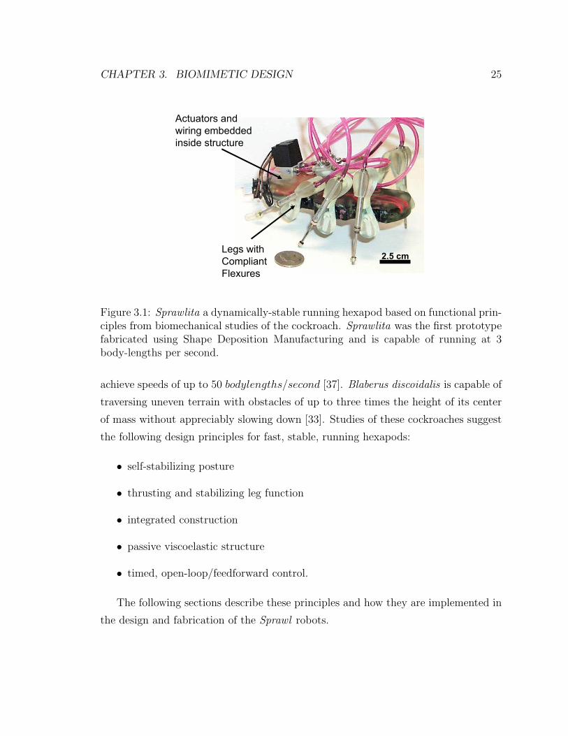
3.1 Sprawlita a dynamically-stable running hexapod based on functional
principles from biomechanical studies of the cockroach. Sprawlita was
the first prototype fabricated using Shape Deposition Manufacturing
and is capable of running at 3 body-lengths per second. . . . . . . . . 25
3.2 Self-stabilizing posture: A rear and low center of mass and wide base
of support contribute to the over-all stability of locomotion . . . . . . 27
xii

3.3 Leg Function Studies of ground reaction forces in cockroach locomotion
show that forces are directed towards the hip joints, essentially acting
as thrusters. In addition, each leg performs a di!erent function: front
legs act as decelerators while hind legs act as accelerators; middle legs
act as both. . . . . . . . . . . . . . . . . . . . . . . . . . . . . . . . . 28
3.4 Shape Deposition Manufacturing process plan for Sprawlita’s legs. The
alternating layers of hard and soft materials, as well as the embedded
components that make up the compliant legs, are shown. . . . . . . . 30
3.5 Leg deflection as shown by high-speed video . . . . . . . . . . . . . . 31
3.6 An alternative leg design allowing deflection in one rotational and one
axial direction. The leg is a spatial fourbar with compliant segments
that allow the sti!ness in each direction to be tuned independently. . 31
3.7 Suggested roles of a feedforward motor pattern, preflexes, and sensory
feedback. Here, disturbance rejection is the result of the mechanical
system and not an active neural control loop. (Adapted from [35].) . 33
3.8 Robot performance test results for slopes ranging from -8 degrees down-
hill to 20 degrees uphill for two di!erent stride periods. These tests
indicate the need to adapt variables of the locomotion scheme to envi-
ronmental conditions. . . . . . . . . . . . . . . . . . . . . . . . . . . . 35
4.1 Overview of simulation of Sprawlita featuring passively compliant hips
and pneumatic thrusting legs . . . . . . . . . . . . . . . . . . . . . . 41
4.2 (a) Overview of hip model and (b) the step deflection response for both
the robot leg and the model . . . . . . . . . . . . . . . . . . . . . . . 44
4.3 A comparison of the pressure rise and ground reaction force for the
robot and the model . . . . . . . . . . . . . . . . . . . . . . . . . . . 45
4.4 Schematic for the ideal gas pneumatic pressure model. The mass of
the air mair, extension of the piston x and pressure in the piston p
are all states of the system and are computed at each time step of the
simulation. . . . . . . . . . . . . . . . . . . . . . . . . . . . . . . . . . 46
xiii

4.5 A comparison of the exponential (case 1) and ideal gas (case 2) models
of Sprawlita’s pneumatics. Figure (a) compares the pressure profiles
for two strides, and (b) shows the front leg vertical ground reaction
force for the same strides . . . . . . . . . . . . . . . . . . . . . . . . . 48
4.6 Velocity vs. stride period for model and robot . . . . . . . . . . . . . 52
4.7 Ground reaction forces for each leg of robot and model . . . . . . . . 53
5.1 The e!ect of altering the valve stride period on locomotion e"ciency. 57
5.2 Velocity Profiles for Actuation Parameter Variations . . . . . . . . . . 64
5.3 Velocity Profiles for Body Parameter Variations . . . . . . . . . . . . 66
5.4 Velocity Profiles for Environmental Parameter Variations . . . . . . . 67
5.5 Speed and stability as a function of leg orientation . . . . . . . . . . . 70
5.6 Speed and Stability as a function of leg orientation . . . . . . . . . . 71
5.7 E!ect of ground contact sti!ness on the velocity for various stride periods 75
5.8 Range of leg angles chosen for terrain adaptation tests . . . . . . . . 78
5.9 E!ect of varying the mean leg angle on the velocity of the model for
various terrain conditions . . . . . . . . . . . . . . . . . . . . . . . . . 79
5.10 E!ect of Leg Hip Sti!ness on Velocity for Outdoor Sprawl . . . . . . 81
5.11 E!ect of Leg Angle on Velocity for Outdoor Sprawl. Each grid location
represents a di!erent nominal configuration of the robot. Each point
is where the lines of action of the leg pistons intersect. The circle’s
radius at each point is proportional to the robot’s velocity at that
configuration. The shaded area represents the unstable region. . . . . 83
6.1 Diagram showing how the WSM is calculated and how the 33 mm
threshold relates to the geometry. . . . . . . . . . . . . . . . . . . . 90
6.2 E!ect of leg angle on simplified WSM. The dark line represent the
boarder of instability as defined by ‘nose diving’ and the WSM respec-
tively. The size of the circle represents the open-loop forward velocity
for (a) and the magnitude of the WSM (b). . . . . . . . . . . . . . . 91
6.3 Typical decline in the WSM for an unstable configuration . . . . . . . 92
xiv

6.4 E!ect of altering hip sti!ness on velocity for a range of leg angles: (a)
For the softest hips tested, (b) For optimal sti!ness selected in section
5.5, and (c) for the sti! value tested. (d) shows the peak velocity for all
configurations at each level of sti!ness tested. (e) shows the fraction of
the tested configurations at each sti!ness that resulted in fast, period-1
running. . . . . . . . . . . . . . . . . . . . . . . . . . . . . . . . . . . 93
6.5 How intermittent foot contact digitally di!erentiates rough terrain, and
the concept of a ‘characteristic slopes’ for a given terrain . . . . . . . 96
6.6 E!ect of leg angle on bands of slope . . . . . . . . . . . . . . . . . . 97
6.7 E!ect of leg angle on bands of slope . . . . . . . . . . . . . . . . . . 99
6.8 E!ect of leg angle on bands of slope . . . . . . . . . . . . . . . . . . 101
6.9 Perturbation response for Pitch and Roll . . . . . . . . . . . . . . . . 103
6.10 Perturbation response for yaw rate and velocity . . . . . . . . . . . . 104
6.11 E!ect of leg angle on perturbation settling time . . . . . . . . . . . . 105
6.12 Comparison of the e!ect of leg posture for di!erent stability measures.
The circles represent the magnitude of the WSM for each of the stable
configurations. . . . . . . . . . . . . . . . . . . . . . . . . . . . . . . . 108
A.1 (A) Picture of the hip flexure test set up indicating the locations of
the markers, and (B) a typical picture of the motion of the markers in
Cartesian space. . . . . . . . . . . . . . . . . . . . . . . . . . . . . . 115
A.2 Six step responses. . . . . . . . . . . . . . . . . . . . . . . . . . . . . 116
A.3 Figure showing the surface friction test set up . . . . . . . . . . . . . 116
xv

Chapter 1
Introduction
For most of the history of the world legs have been mankind’s primary means of
transportation. While wheels have been incredibly useful in innumerable tasks, it is
only with the advent of the steam engine that self-powered wheeled vehicles came
into their own. Up until that time terrestrial locomotion was legged locomotion. And
legged locomotion meant a muscle based power source. We walked, we rode horses,
we pulled wagons, but we always used legs.
With the advent of the railway and the automobile the mechanical engineer came
into his own. Thousands of miles of track were laid, and later millions of miles of
roads were paved. The automobile has so permeated our culture that ‘walking’ and
‘running’ are considered recreational pastimes!
Nevertheless there are a lot of places that cars can not go. Consequently re-
searchers have, despite the di"culties, attempted to create artificial or robotic walk-
ers and runners. Over the past quarter century substantial progress has been made in
robotics in general. Many of these advances have carried over to legged locomotion,
but some inherent properties of legged motion have limited the successes in utiliz-
ing the traditional position and force base control techniques used in other areas of
robotics.
The purpose of this thesis is to put forward the design, simulation, and analysis of
a class of biologically inspired running robots. This analysis argues that the ease of
design and control, as well as the performance of running robots can be dramatically
1

CHAPTER 1. INTRODUCTION 2
improved with an appropriately designed self-stabilizing structure. While the robots
described in this thesis do not yet qualify as the “greatest thing since the wheel”
for the field of locomotion, I believe that the principles examined represent one step
toward making a viable artificial running machine.
1.1 Motivation
There are a number of advantages inherent to legged systems, the foremost of which
is their flexibility in dealing with rough terrain. They can step over pits or obstacles,
they can turn rapidly, and they lend themselves to climbing, swimming, burrowing,
and a host of other activities. These are all activities that we humans and many
other animals do relatively e!ortlessly. The challenge now for roboticists is to create
machines that duplicate the mobility and agility of living creatures.
A large percentage of earth’s surface is unavailable to wheeled vehicles. Much of
this area is, perhaps consequently, unpopulated. Nevertheless there are often com-
pelling reasons to send autonomous vehicles into these areas. Volcanos, surf zones,
densely wooded areas, caves, and mountainous regions are all possibly o!-limits to a
wheeled or tracked vehicle. Nevertheless for exploration purposes it would be ideal
to have a class of vehicle that did not need (or make) its own road. One example of
an early commercial interests is in the logging industry where a legged harvester is
being developed by Plustech, a John Deere company.
In addition to wilderness areas, there are environments made hostile due to man-
made e!ects such as mine fields and urban disaster sites. In these situations, sending
in humans is dangerous, yet their locomotive flexibility is required. One can also
imagine a number of scenarios involving surveillance, security, or planetary explo-
ration where having a vehicle with animal like invariance to terrain would be ideal.
1.2 Challenges
To solve the problem of getting from here to there (locomotion), engineering and
technology have favored solutions such as the wheel that have radically departed

CHAPTER 1. INTRODUCTION 3
from biological examples. In doing so they have exploited the strengths of their
discipline including the ability to produce accurate, repeatable, uniform geometric
parts, smooth bearing surfaces, and rotary actuators.
Creating e!ective legged robots, however, requires moving more directly into the
domain of motion that is favored by animals. Some inherent di"culties with legged
systems include: intermittent contact with the ground, interaction with an unknown
environment, unexpected environmental disturbances, and more complicated mechan-
ical dynamics. Relative to these demands, most mechanical attempts to created
legged robots have resulted in slow, fragile, or unstable systems.
Animals mitigate these di"culties in a number of ways including: a sophisticated
vision system for obstacle detection, a vestibular system to sense balance, a central
controller or brain to perform path planning, a distributed reflex system to regulate
gaits, and passive compliance in the legs to help in stabilization.
Researchers have worked for years to create artificial vision systems, inertial sen-
sors, and controllers for planning and gait generation. Determining the role of passive
compliance in augmenting stability has, however, been comparatively underdeveloped.
This thesis argues that by understanding and utilizing the way in which animals use
the passive compliance and energy dissipation in their leg structures the overall task
of achieving fast and stable running can be greatly simplified.
1.3 Contributions
The main contribution of this thesis is to characterize under what conditions an ap-
propriately tuned passive physical system can allow legged robots to run over rough
terrain with purely open loop control. The development and analysis of the Sprawl
family of robots demonstrates that a proper mechanical structure is not only neces-
sary, but can in fact be su"cient for robust outdoor locomotion.
The construction and use of a detailed dynamic simulation of the robot has allowed
the passive dynamic stabilizing properties of the legs or “preflexes” [18] to be tuned to
double the robots speed. For robust operation however, stability as well as speed needs
to be improved. Characterizing stability over rough terrain is a di"cult task, and

CHAPTER 1. INTRODUCTION 4
there is currently no universal metric for measuring it in such situations. Consequently
in this thesis a number of measures for gauging the impact of design changes on
stability are put forward and compared.
Specific contributions of this thesis include:
• Design and construction of the first monolithic multi-material compliant SDM
legs for the Sprawl robots.
• Development and calibration of a three-dimensional multi-body dynamic sim-
ulation of the Sprawl family of robots, and demonstration that the simulation
can be used to dramatically improve the design.
• Characterization of the parameter space for self-stabilizing leg posture.
• Evidence that a sprawled for-aft leg posture and di!erential leg use, increase
the range of fast and stable operation.
• Demonstration of how increasing hip impedance increases stability and charac-
terization of its e!ect on the velocity of the robot.
• First direct comparison of the e!ect of varying robot parameters for multiple
stability measures (including perturbation response rate and a dynamic stability
margin) on a running robot.
1.4 Thesis Overview
Chapter 2 gives an overview of previous work in walking and running robots. Special
attention is paid to the approaches taken to measure and generate stable gaits. The
concept of stability margins for walking robots is discussed, as is return-map analysis
for simplified hopping and walking systems. The context for the present work is given
in terms of the most recent developments in building and controlling running robots.
Chapter 3 describes the design of the Sprawl family of running robots developed
and analyzed in this thesis. The biological findings that motivated their construction
are reviewed, and the manufacturing process that enabled the construction of the

CHAPTER 1. INTRODUCTION 5
multi-material complaint legs is briefly summarized. The chapter concludes with a
discussion of initial results from a parameter variation design of experiments, which
indicate the relative importance of actuation and stance parameters on performance,
and how strongly these parameters are coupled.
Chapter 4 describes the construction and calibration of a three dimensional dy-
namic simulation of the robot used to evaluate design changes. The model was de-
signed to be as simple as possible while maintaining su"cient fidelity to the robots
for predictive purposes. The experimental tests used to characterize the model com-
ponents are described as are comparisons between the behavior of the robot and
model.
Chapter 5 describes how the simulation was used to investigate the parameter
space and tune the performance of the robot. The robot’s energetics and sensitivity
to parameter variation are described, as are the e!ect of varying environmental pa-
rameters on speed and e"ciency. Critical leg parameters and couplings are identified.
The chapter concludes with a description of how the simulation was used to redesign
the robot’s legs, doubling the robot’s speed.
Chapter 6 investigates the shape of the parameter space that results in self-
stabilizing running, and how changing these parameters a!ects the robot’s perfor-
mance. Four distinct measures for running ‘stability’ over rough terrain are presented.
The e!ects of changing the leg posture and hip impedance on each of these criteria
are compared.
Chapter 7 gives some conclusions and suggestions for future work.

Chapter 2
Previous Work
This chapter gives an overview of some of the previous research on legged robots,
with an emphasis on the e!orts that have led toward fast, stable locomotion, espe-
cially over rough terrain. The first section describes some significant walking robots
and the designs and controllers they have used to achieved motion. Di"culties with
rough terrain have led to a number of approaches to generating and coordinating leg
trajectories. Robots have implemented a variety of strategies, from centralized force-
control algorithms to decentralized, reflexive controllers to rule-based and adaptive
controllers. The overview of walking robots concludes with a discussion of the mea-
sures or “margins” that have been developed to quantify stability, and to help avoid
configurations and motions that would lead to falls.
The next section discusses dynamic and running systems, including simple hop-
ping robots and passive dynamic bipeds. These simple systems are designed so that
their inherent dynamics can be utilized to help stabilize themselves or to develop
energetically e"cient controllers. Additionally, these simple systems allow for the use
of reasonably simple and tractable models to guide their design and analyze their sta-
bility. Included is a very brief overview of the return-map stability analysis technique
used on these systems.
The concluding section looks at multi-legged running systems, most of which have
been developed concurrently with the research described in this thesis. These fast
and stable runners have come the closest to achieving performance levels necessary
6

CHAPTER 2. PREVIOUS WORK 7
for practical application in areas such as de-mining, planetary exploration, forestry,
surveillance, and search and rescue.
Since these robots are generally too complex to allow an analytic analysis of their
dynamics and stability, a number of approaches have been used to achieve stable
locomotion. These methods are discussed, giving context to the approach described
in this thesis.
2.1 Walking Robots
2.1.1 Early Walkers
In the days before microprocessors were powerful enough to implement sophisticated
control systems, a number of techniques were used to stabilize walking machines.
These techniques relied on human feedback, clever mechanical design, or simple feed-
forward trajectories. The principles embodied in these machines are of particular
interest due to their renaissance (in modified form) in some of the most recent and
successful running robots.
Teleoperation
An ingenuous approach to controlling a walking machine was taken by the GE Electric
Walking Truck built in 1967 [75]. It used human teleoperation to control and stabilize
itself. Built to extend the functional reach and power of a human, it was, in e!ect,
a quadrupedal mechanical exoskeleton. While the Walking Truck was functional,
researches quickly found that coordinating and controlling so many degrees of freedom
was a di"cult and demanding task which quickly exhausted the operator. Although
GE abandoned the project, it did demonstrate impressive performance by leveraging
properties of the human body.
Simple Trajectories
In the 1970s and early 1980s, the level of computational power available was insu"-
cient to implement intricate behaviors on complex geometries. Consequently, the first

CHAPTER 2. PREVIOUS WORK 8
generation of computer controlled walking machines including the Phoney Pony and
the OSU Hexapod had two and three degrees of freedom per leg and were able to fol-
low only very simple, pre-programmed trajectories [89]. These simple motions were
su"cient to generate forward movement, but the rigid legs fared poorly on rough
terrain. The proliferation of walking toys and ‘robotic hobby kits’ based on these
principles, demonstrates the success of this approach and its limitation to smooth
surfaces and slow speeds.
Beam Walkers
A less biological, but simpler approach to building stable legged robots was taken by
Ambler [62] and the Walking Beam [26]. Structurally, both of these machines moved
like two nested tables where one set of legs could translate while the other was in
contact with the ground. Thus one set of legs could support the body, while the
retracted set could be positioned for the next step. Designed to go to Mars, their size
and wight proved to be prohibitive. A smaller version of a frame walker, Dante II,
did succeed in climbing into a volcanic crater on Mt. Spurr in 1994 [10]. Its fragility,
however, proved to be its undoing as it had to be pulled out with its tether after
breaking on the rough terrain.
Despite their limitations, these robots could handle some pretty rough terrain.
Though these robot designs are now outdated, some of the principles they embodied,
such as the use of simple trajectories and alternating tripod gaits have been recently
revisited by a number of running robots.
2.1.2 Centralized Controller
As computational power and the sophistication of controllers increased during the
1980s, so did the complexity of the structures they were asked to direct. One excellent
example of a sophisticated walker is the Adaptive Suspension Vehicle (ASV) [97],
which had six legs each with three degrees of freedom. It was powered by a motorcycle
engine and was able to carry its operator.
The ASV was able to walk outdoors, up and down shallow slopes and even over

CHAPTER 2. PREVIOUS WORK 9
railroad ties. It used a variety of techniques including a primitive vision system and
a ‘follow the leader’ gait to implement obstacle avoidance behaviors [74]. Drawbacks
to the ASV included its noise, rough ride, extreme cost, and complex control require-
ments.
The clever use of a pantograph mechanism in the leg decoupled the control of
the leg degrees of freedom. This deviation from a biological leg design allowed the
height, extension, and rotation of the leg to be independently controlled, greatly
simplifying the control problem. The computational burden was further reduced by
the implementation of a control scheme based on “zero foot interaction forces” [102].
Despite using these techniques the control of the ASV remained a computationally
intensive task.
2.1.3 Gait Generation Via Distributed Control
The experience with the ASV and other robots with complex structures and many
degrees of freedom in the legs, demonstrated the di"culty in developing robust control
systems to coordinate multi-leg motions.
Brooks and his students at MIT have argued that implementing a distributed
control system is the answer, and supported this claim by building a series of small
robots including Attila [5], Gengis [6], and Boadecia [14].
As a source of inspiration for designing distributed control systems, Brooks and
other researchers have turned to biology. Due to their relatively simple physiology,
investigation into insect locomotion, particularly the stick insect, has been very fruit-
ful in developing simple, distributed controllers which generate natural gaits. Cruse
in particular has identified a number of low-level reflexes that work together to coor-
dinate the timing of the thrust and retraction of insects legs [28].
Some examples of robots that have used these principles include CWRU robot I
[31] and II [30], and the TUM Robot [81]. These small (0.3 to 0.6 m long) hexapedal
robots are capable of slowly walking over rough terrain and even a slotted surface.
They use foot contact sensors and simple microprocessors to implement their reflex
coordination and foot placement algorithms.

CHAPTER 2. PREVIOUS WORK 10
Despite these advances, the generation of smooth and natural walking motions
has still proven di"cult to achieve through discrete rules. Several researches have
attempted to mimic nature or the brain in a more centralized manner. One approach,
attempted with the hexapod Lauron, was to implement a motion controller based on
neural networks [12], another approach attempted by Galagher was to use genetic
algorithms to evolve the controllers [38].
Most recently Klaasen et al. have used “Basic Motion Patterns” derived from
reflexes and neural networks to generate gaits for their octapedal robot Scorpion.
They found that its walking patterns were comparable to those found in real scorpions
[56]. In a similar vein, the robot Tekken has augmented a central pattern generator
(CPG) and reflex based controller with legs equipped with virtual spring-dampers
designed to mimic the viscoelastic properties of muscle. This autonomous quadruped
can walk over terrains with “medium degrees of irregularity” [32].
The generation of smooth and stable walking trajectories has developed gradually
over time. The use of biological principles in the design of the robots and controllers
has helped considerably. We are just now beginning to be able to create fluid walking
gaits over rough terrain. In addition to being smooth, these gaits need to guarantee
stability. To aid in this a number of stability measures or “margins” have been
developed over the years.
2.1.4 Static Stability Margins
Slow moving or quasi-static robots are stable as long as the ground projection of the
center of mass (GCOM) of the robot lies within the polygon of support defined by the
stance legs. A measure of stability called “Static Stability Margin” (SSM) has been
defined by McGhee [66] to be the minimum distance from the GCOM to an edge of
the support polygon. This is shown schematically on figure 2.1.a.
A variant of SSM, the “Longitudinal Stability Margin” (LSM) is given by the
distance along the ground in the sagittal plane from projections of the center of mass
to the front edge of the support polygon [106].
These stability margins, however, do not account for slopes or other irregularities

CHAPTER 2. PREVIOUS WORK 11
Static Stability Margin (SSM) Energy Stability Margin (ESM)
)(min i
l
iESM mghSs
=
ψθ cos)cos1( −= ii Rhwhere
SSM
LSM
hi
Ri
θ ψ
Figure 2.1: Static Stability Margin (SSM) and Energy Stability Margin (ESM) Il-lustrated. The polygon of support is depicted as a gray triangle. The SSM is thedistance from the ground projection of the center of mass of the robot to the nearestedge of the support polygon. The LSM is the sagittal projection of the SSM. TheESM indicates the amount of potential energy (proportional to hi) that needs to beovercome before tipping occurs. Thus slope and body height are explicitly considered.
of terrain or the height of the center of mass of the robot. An improved and more
practical measure called the “Energy Stability Measure” (ESM) was proposed by
Messuri [71], and is shown schematically in figure 2.1b. The ESM measures how
much potential energy needs to be overcome before the robot tips. Essentially, this
measures how much the center of mass must rise during tipping before it exits the
support polygon. Mathematically this is given by:
SESM = minlsi (mghi) where hi = Ri (1" cos!i) cos"i (2.1)
Where m is the mass of the robot, g is the gravitational constant and hi is the
height the center of mass can rise before the robot tips along the ith edge of the
support polygon. R is the distance between the COM and the ith edge of the support
polygon, and ! is the angle between Ri and the gravity vector. "i indicates inclination
of the ith edge of the support polygon with respect to its projection onto the plane
normal to the gravity vector.
A version of this measure (scaled by mg), called the “Normalized Energy Stability
Margin” (NESM) [46] was successfully implemented by Hirose on Titan VII [47]. This
robot utilized a controller that modified its stance posture to maximize the NESM

CHAPTER 2. PREVIOUS WORK 12
and was able to negotiate slopes of up to 30 degrees.
2.1.5 Dynamic Stability Margins
The static stability margins described in section 2.1.4 are only valid for robots trav-
eling very slowly, typically using a wave or crawl gait. To incorporate the e!ect of
the dynamics on the stability of robots moving at more than ‘quasi-static’ speeds, a
number of alternative stability margins have been proposed.
Center of Pressure
By tracking the distance from the instantaneous center of pressure (COP) instead of
the GCOM of a robot, a more accurate stability margin can be generated. The COP
is the location of the resultant ground reaction force in the contact plane, (as shown
in figure 2.2) and can be expressed mathematically as:
#OP =
!ni=1 qifni!ni=1 fni
(2.2)
Where OP is the position vector from the origin to the COP, fni is the normal
component of the ground reaction force at the ith foot, and qi is the position vector
from the origin of the coordinate system to the point of contact of the ith foot. The
distance from the nearest edge of the polygon of support to the COP has been termed
both the “Dynamic Stability Margin” [79], and the “E!ective Mass Center” [54] as it
takes into account some of the dynamics of the mechanism as well as its kinematics.
Comparison
Over the years a number of other stability margins have been proposed. Only recently
has a study been undertaken by Garcia to analyze the relative merits of these defini-
tions [39]. She compared six di!erent margins for six cases of a simulated quadruped
walking in various conditions and found that each measure can give a di!erent in-
stant of maximum stability depending on the test condition; no single criterion gives
the optimal or most reliable results for all of the test conditions. Nevertheless this

CHAPTER 2. PREVIOUS WORK 13
DSM
COP/EMC
qi
OP
fi
COP/EMC = Center of Pressure or Effective Mass Center OP = position vector from the origin to the COP/EMC fi = ground reaction force at the i-th footqi = position vector from the origin to the point of contact of the i-th foot
Figure 2.2: The dynamic stability measure is the distance from the center of pressure(COP) or “E!ective Mass Center” (EMC) to the nearest edge of the support polygon(shown in gray).
investigation was the first to shed some light on di!erences between these measures.
One shortcoming of this study for the present work was that all of the tests only
considered four-legged walking gaits.
2.1.6 Bipedal Walking Stability
All of the walkers discussed thus far have been multi-legged, which allows gaits with
relatively large stability margins. While this eases the stability problem, people have
continued to pursue the dream of an anthropomorphic robot. In fact, the increased
di"culty of getting a two legged machine to walk has spurred the development of
more sophisticated and sensitive controllers.
In 1970 Vukobratovic proposed using what he called the “Zero Moment Point”
(ZMP) to help stabilize a biped [101]. Schematically the location of the ZMP with
respect to an arbitrary origin is shown in figure 2.3. Mathematically the ZMP is
defined as:

CHAPTER 2. PREVIOUS WORK 14
ZMP
OZ
OCi GiFi
Mi
OZ = position vector from the origin to the ZMPOCi = direction vector from the origin to the mass center of the i-th linkMi = moment of the inertial force of the i-th link about its mass centerFi = inertial force of the i-th link about its mass centerGi = gravitational force of the i-th link about its mass center
Figure 2.3: The Zero Moment Point is the point in the support plane where theresultant inertial force must act so that the magnitude of the out-of-plane resultantmoments are zero. If the robot is not tipping, then this is the same point as the centerof pressure.
"
OZ#n#
i=1
(Fi + Gi)
$
h
=
"n#
i=1
OCi # (Fi + Gi) +n#
i=1
Mi
$
h
(2.3)
Where OZ is the position vector from the origin to the ZMP and OCi is the
position vector from the origin to the mass center of the ith link. Mi is the moment
of the inertial force, Fi is the inertial force, and Gi is the gravitational force. Each of
these is computed about the corresponding mass center for each link.
As long as the ZMP is within the polygon of support then it is coincident with
the COP. The di!erence is that the ZMP is computed from the link accelerations
rather than the ground reaction forces (GRF). This allows the use of centeralized
proprioceptive sensors to compute the robot’s stability.
Recently Goswami reformulated the ZMP in terms of the forces acting on the ankle
of the stance foot (for a biped) and called the distance from the edge of the support
polygon to this point the “Foot Rotation Index” (FRI) [43]. He also suggested that
when this point is outside of the polygon, it serves as a measure of instability.
A number of walking robots have used the ZMP, or a variant of it, in their control

CHAPTER 2. PREVIOUS WORK 15
scheme include Honda’s Asimo [45, 107]. However, none of these robots have been
able to demonstrate good performance over rough terrain. This is partially due
to the fact that when having a single rigid foot in contact with a rough surface a
small pressure shift may dramatically change the ground-foot interaction mid-stride,
instantly destabilizing the robot.
Other approaches to walking controllers have included an ‘intuitive’ approach
attempted by G. Pratt and J. Pratt at MIT. They specified specific aspects of walking
that needed to be achieved with each stride and wrote simple controllers to ensure
that each of these happened. This control scheme was successfully implemented on
Spring Flamingo [84].
They have also used a neural net to stabilize a biped in simulation. The neural
net helps to account for the unmodeled dynamics and has demonstrated Lyapunov
stability [51]. They continued this work with the development of a “Virtual Model
Control” to allow a planar biped to walk on unknown slopes (and by extension)
rough terrain with minimal sensing [83]. The implementation of these control schemes
has increased the robustness of the biped on unstructured terrain, but they are still
constrained to slow motions.
2.1.7 Walking Constraints
Most of the robots described up to this point have been composed of rigid links artic-
ulated by motor-encoder feed-back loops. Consequently, they are precise, repeatable
and have large workspaces, but are slow. To go faster requires understanding and
accounting for the dynamics of the system as well as for the significant and sometimes
unpredictable impulses from foot contact. Robots in general are therefore limited not
only by the computational power available, but more fundamentally by their sensor
and actuator bandwidths. For many motions this constraint is not significant, but for
fast legged locomotion, which is characterized by large and unpredictable impacts,
this limitation is critical.

CHAPTER 2. PREVIOUS WORK 16
2.2 Dynamic Locomotion
Running involves more than simply moving faster than walking. It usually involves
a change of gait and aerial phases during which no feet are on the ground. A more
rigorous definition of running can be formed by looking at the relative phase of the
kinetic and potential energy during a gait [20]. McMahon [67] describes two simple
models that have been widely used to capture walking and running. The stance
leg in walking is modeled as an inverted pendulum, with the potential energy being
the greatest at the top of the swing, and the kinetic energy greatest just before the
stride transition. Running is modeled as a spring-loaded inverted pendulum (SLIP)
where potential energy is stored in the axial leg spring during stance. This model
also allows for the possibility of flight phases between steps. These models have been
found to have good correlation with a wide range of observed human and animal
ground reaction forces [15, 68].
Full et. al [35] have hypothesized that the SLIP model constitutes a fundamen-
tal template for dynamic locomotion. They suggests that this pogo-stick type hop-
ping motion captures some of the essential dynamics found in all running systems.
Alexander has suggested that the use of mechanical springs in running helps reject
disturbances, return energy to the system, and can help ease control [2].
2.2.1 Hopping Robots
The earliest successful dynamic running robots were built by Raibert and his students
at CMU and later at MIT [87]. The first planar hopping monopod created in 1980
[87] was a pneumatic air piston/spring that was controlled by three simple control
laws. Raibert assumed that hopping height, forward velocity, and pitch could be
controlled independently. Simple laws were put forth to correlate hopping height to
the magnitude of thrust, velocity to the touch-down angle of the leg, and body pitch
to the hip servoing during stance. Though these motions are, in fact, coupled, the
decoupled controllers were elegantly simple and turned out to be ‘close enough’. The
robot was able to run at speeds up to 2.3 m/s, hop up stairs and a biped version could
even do a flip [48]. One limitation was that the initial planar runner required complete

CHAPTER 2. PREVIOUS WORK 17
and accurate state information acquired by seven sensors in order to implement this
control scheme.
The remarkable success of these hoppers spawned an analytic study of simple
hopping robots and their stability. Koditschek found that their dynamics were very
similar to those of juggling robots [57], and both systems can be analyzed in closed-
form using return maps and the eigenvalue analysis described in section 2.2.3 [19]
[95]. Mombaur [72] extended this analysis to the case of planar hopper, and Cham
[21] furthered this work by removing the assumptions of low damping and no gravity
during stance.
Variants of hopping robots that have been built include an energy e"cient variant
of a hopping monopod, called the Bow-legged Hopper, developed at CMU. This hopper
used a very e"cient compliant leg which could store and return 70% of the energy from
each bounce [17]. An alternative approach taken by Ahmaid and Buehler involved
using both the hip and leg actuator to stabilize the trajectory while preserving the
passive motion. This approach dramatically reduced the required actuation energy
at the hip [1].
In addition to increasing the e"ciency of hoppers, work has been done to increase
their stability. Ringrose, for example, built an entirely open-loop self-stabilizing hop-
ping robot based on curved feet and a feed-forward actuation scheme [88].
The relatively simple dynamics of hopping and promising early experimental suc-
cesses have led to the development of a remarkable set of robots that have been the
first to achieve fast and stable motion.
2.2.2 Passive Dynamic Bipeds
In parallel to the research on hopping robots, work has been done investigating the
passive dynamics of simple bipedal walkers. McGeer has demonstrated analytically
and experimentally that a completely passive set of rigid links can walk down a gentle
slope, powered only by gravity [65]. This remarkable achievement demonstrates the
importance of understanding and utilizing the inherent dynamics of a legged system.
Others including Garcia [40], Goswami [42], and Kuo [61] have followed this with

CHAPTER 2. PREVIOUS WORK 18
studies of these simple bipeds utilizing a stability analysis similar to that used for
hopping robots (as described in section 2.2.3).
More recently several groups of researchers have exploited the concept that utiliz-
ing the natural dynamics of walking can lead to energy e"cient and stable gaits with
minimal control e!ort. These attempts at “passivity-mimicking” have included work
by Asano [7], Ohta [77], and Ono [78].
2.2.3 Stability Analysis for Simple Dynamic Systems
The simple hopping and walking models described in sections 2.2.1 and 2.2.2 have
allowed for the analytical (or at least numerical) computation of system stability by
means of an eigenvalue analysis of return maps.
Return maps are functions that describe how an oscillatory or repeating function
changes from one cycle to the next. For walking these have also been called “step
functions” [65], since they describe the how state of the system (q) changes from step
to step, i.e. qn+1 = f(qn). In nonlinear dynamics language, a steady-state gait is
seen as a stable limit cycle or “fixed point” (q!) on the return map. This implies
that all of the elements of the state vector (except forward position) are the same
from one step to the next, i.e. q! = f(q!). When a return map can be found,
either analytically or numerically, and evaluated at fixed points, an analysis of the
eigenvalues and eigenvectors of its Jacobian indicates the shape of the local basin of
attraction for the trajectory.
Jf (q!) =
$f
$qn
%%%%%q!
=$qn+1
$qn
%%%%%q!
(2.4)
Where Jf (q!) is the Jacobian of the return map evaluated at the fixed point (q!).
Since each step or cycle is discrete event, if absolute values of all of the eigenvalues
are less than one, the trajectory is stable. The magnitude of each eigenvalue indicates
the slope in its corresponding direction (eigenvector), or the percentage decay from
one step to the next. This is a local measure of the slope for the basin of attraction.
An advantage of this technique is that it incorporates the e!ect of perturbations from
all directions and on all state variables in a single measure [94].

CHAPTER 2. PREVIOUS WORK 19
This analysis technique is general and can be applied to a number of non-linear
systems including running [36], but thus far has only been successfully used on simple
models. The most applicable of these to this work is Chams’s analysis of planar
hoppers. The results of this study inspired a scheme to tune the valve actuation
pattern of Sprawlita [23].
2.3 Multi-legged Runners
Most recently a number of researchers have shown that fast locomotion over rough
terrain can be achieved by building platforms combining the advantages of a springy
hopper with the stability of a multi-legged platform.
There are a number of potential biological models for designing a compliant multi-
legged runner. The two most popular classes are mammalian runners, such as dogs or
horses, which generally have four long vertical legs and narrow posture, and arthro-
pods which tend to be smaller, have low centers of gravity, six legs, and a sprawled
postures.
2.3.1 Mammalian Runners
Recent studies of mammal-like running include the work done by Berkemeier [11] who
looked at a 2-DOF quadruped hopping in place with bound and pronk like gaits. He
found that a dimensionless inertia of 1 was essential for a stability of the bound. (Any
roughly mammalian multi-legged structure will have the requisite inertial properties.)
Buehler et al. have developed Scout, a quadruped that utilizes compliant legs and
actuated hips. The platform has been used to analyze a number of control schemes
and gaits from a “Walking Bound” with constant hip velocities during stance [29], to
a trot, and even to gaits with gallop-like footfall patterns [82].
Currently under development is a galloping machine designed to have kinematics
inspired by the Nubian goat. This robot is designed to run with an asymmetric foot
fall pattern to investigate high speed galloping gaits. It features electric actuation,
distributed controllers, and low inertia complaint legs [76]

CHAPTER 2. PREVIOUS WORK 20
2.3.2 Arthropod Runners
Developed concurrently with the Sprawl robots described in the next chapter, RHex
[92] is a half meter long autonomous hexapedal running robot built on biological
principles similar to the ones described in this thesis. It demonstrates the possibility
of simple, robust dynamic running machines that rely heavily on passive dynamics
and an open-loop gait. It can run at more than 5.0 bodylengths/second and over
rough terrain. Its controller has been modified to allow it to pronk and go up steep
slopes [58], climb stairs [73], right itself [93], and even swim. It has come closer than
any robot to date to achieving autonomous mobility in unstructured terrain.
2.4 Stability in Multi-legged Runners
Stable running is inherently di!erent and in many ways more di"cult than stable
walking. The increase in speed and the gait patterns used in running result in dynamic
e!ects that cannot be ignored: larger momentum, shorter response times, and large
impacts at ground contact.
At first glance it appears that achieving a stable gait in a multi-legged runner is
simpler than for a hopping monopod since statically stable configurations are possible.
However, the additional complexity of the multi-limbed structure makes the direct
application of the closed form control solutions and the functional approximations
that worked well for monopods impossible except for a small class of physical designs.
Despite the fact that statically stable configurations are possible during running,
none of the stability margins described in sections 2.1.4 and 2.1.5 is applicable for
fast dynamic running systems, since even robots with wide postures have airborne
phases and can violate the ‘dynamic’ stability margin with each stride. The return
map stability analysis methods described in section 2.2.3 has only been succesfully
applied to simple systems, such as one-legged hoppers, and even then they only give
the slope of the basin of attraction around the fixed point.
In short, there is no universal measure for the dynamic stability of a complex
system running over rough terrain. An e!ort to begin to remedy this situation is

CHAPTER 2. PREVIOUS WORK 21
described in chapter 6.
Even without the ability to directly analyze or measure the stability of a system
it is still possible to build controllers and robots that run well on rough terrain. It
appears that outside of the body of research with which this thesis is associated,
there are two main approaches that have been used to build fast and stable robots,
implementing complex controllers and mapping to simple models.
2.4.1 Complex Controllers
The first approach to dealing with the di"culties associated with controlling complex,
multi-legged running machines is to use “intelligent” or “adaptive” controllers. This
is the approach taken by the OSU/Stanford hopping leg and galloping goat. They use
a direct adaptive fuzzy controller to deal with the non-linearities, plant errors, and
disturbances experienced by the robot. This system does not require a good model of
the plant or extensive system identification, but instead uses heuristics (105 rules) as
the basis for the controller. Thus the system can make use of the natural dynamics
of the system and can generate gait characteristics comparable to their biological
inspiration [63]. The downside to this method is that is something of a ‘black box’
type approach and it is di"cult to know exactly what the controller is doing to ensure
stability.
2.4.2 Mapping to Simple Models
Raibert has extended his three part control scheme for hopping robots to bipedal
and quadrupedal running by means of controlling a “virtual leg” [87]. By exploiting
symmetry, the structure of the biped and quadruped are essentially simplified to that
of a monopod. The two or four legs are constrained to act together and are treated for
control purposes as a single leg operating at the center of the robot. The three-part
control scheme that worked for the hoppers is applied to the virtual leg and the biped
or quadruped is able to trot, pace, and bound [86].
Although it does not explicitly use symmetry in its design and control, RHex has
been shown (when loaded) to achieve center of mass trajectories which match the

CHAPTER 2. PREVIOUS WORK 22
predictions of the SLIP model [3]. Furthermore, control strategies for mapping the
six-legged behavior to a single-legged hopper have been developed [90]. These allow
controllers developed for the known dynamics of the simple model to be mapped to
those of a more complex robot.
Grizzle et al. have developed a technique similar to Saranli [90] for a multi-link
bipedal system using a control system to force the dynamics to map to those of
2D system that allows the application of linear tools for evaluating stability. These
include two basic ideas: “Virtual Constraints” and “Hybrid Zero Dynamics” [25,
44]. These techniques allow the development of provably asymptotic and exponential
controllers [103, 104].
In each of these cases a complex robot morphology has been reduced to a simple
dynamic walking or running model for which direct and provably stable controllers
can be written.
2.4.3 Passive Dynamic Self-stabilization
The methods listed in the previous section, however, inherently rely on feedback stabi-
lization loops which are sensitive to bandwidth constraints for sudden impacts. They
can also only give insight into how to tune the passive dynamics in the dimensions
and directions captured in the simple model. Each of these systems relies on passive
leg springs for stability, but by using a black-box like controller or a simplified model,
the ability to gain insight into how to tune these properties is limited. The SLIP
model can be used to give some idea how to tune the vertical compliance, as has
been done in Rhex [4] and iSprawl [55], but leaves unaddressed the rest of the whole-
body e!ective sti!ness matrix. The reliance upon these control techniques leaves an
impoverished repertoire from which to design the passive dynamics of the system.
A third approach to designing a stable runner is to carefully tune the 3D structure
to exploit both the natural rigid dynamics (like passive walkers), and the impedances
of the individual passive strain elements. This is the approach taken with the Sprawl
family of runners and described in this thesis.
While the mapping of complex systems to simple systems allows the development

CHAPTER 2. PREVIOUS WORK 23
of good controllers, the mapping reduces the design space. This thesis argues that
it is exactly in that space where the passive dynamics of the system exist that make
high-performance and self-stabilization even over rough terrain possible–with only
feed-forward control.
2.5 Summary
A large number of walking and running robots have been developed over the years.
In the process, a great variety of controllers have been created in order to generate
stable gaits, and a number of measures and methods have been designed to analyze
their stability. Nevertheless, until the recent development of biologically inspired
compliant multi-legged runners, no robot has been built that can run well on rough
as well as smooth terrain. These recent robots have demonstrated that a tuned
physical structure is fundamental to achieving this capability. As detailed in chapter
3, the Sprawl family of robots shows that this is not only a necessary condition, but
if tuned properly, can be a su"cient condition for fast stable running.

Chapter 3
Biomimetic Design and Fabrication
of Sprawlita
This chapter outlines the design, construction, and initial testing of Sprawlita, a small
hexapedal running robot based on biological principles. These principles of locomo-
tion, taken from the study of small invertebrates, especially cockroaches, include the
use of thrusting legs, passive hip compliance, and a sprawled posture. Their appli-
cation has resulted in a robot that can run at over 5 bodylengths/second, and over
hip-height terrain. It accomplishes this with an open-loop control scheme, and heavy
reliance upon the stabilizing properties of its passive dynamic structure. The proto-
type robot was fabricated using a manufacturing process that allows many of these
principles to be integrated into the structure of the robot itself, much like the biolog-
ical systems that inspired it (Figure 3.1). The chapter concludes by presenting some
initial experiments investigating the e!ects of changing the structure of the robot and
the open-loop control scheme on the performance of the robot.
3.1 Design Inspiration from Biology
For quick and robust traversal over uneven and uncertain terrain, design inspiration
is drawn from small arthropods. In particular, cockroaches are capable of remarkable
speed and stability. For example, it has been shown that Periplaneta americana can
24
CHAPTER 3. BIOMIMETIC DESIGN 25
Legs with CompliantFlexures
Actuators andwiring embeddedinside structure
2.5 cm
Figure 3.1: Sprawlita a dynamically-stable running hexapod based on functional prin-ciples from biomechanical studies of the cockroach. Sprawlita was the first prototypefabricated using Shape Deposition Manufacturing and is capable of running at 3body-lengths per second.
achieve speeds of up to 50 bodylengths/second [37]. Blaberus discoidalis is capable of
traversing uneven terrain with obstacles of up to three times the height of its center
of mass without appreciably slowing down [33]. Studies of these cockroaches suggest
the following design principles for fast, stable, running hexapods:
• self-stabilizing posture
• thrusting and stabilizing leg function
• integrated construction
• passive viscoelastic structure
• timed, open-loop/feedforward control.
The following sections describe these principles and how they are implemented in
the design and fabrication of the Sprawl robots.

CHAPTER 3. BIOMIMETIC DESIGN 26
3.1.1 Self-stabilizing Posture
The use of a sprawled hexapedal posture has many advantages. Many robots have
been designed with six legs so that they can walk with an alternating tripod gait.
By walking with three non-adjacent legs on the ground at one time, the robot can
constantly ensure static stability. The use of this approach, however, has limited
many of these robots to slow, near-static speeds.
Observations of cockroaches running at high speeds, on the other hand, show that
while they also run with an alternating tripod gait, their centers of mass approach
and exceed the bounds of the triangle of support within a stride [99]. Cockroaches
achieve a form of dynamic stability in rapid locomotion while maintaining a wide base
of support on the ground.
In addition, Kubow and Full [35] suggest a further advantage to an appropriately
sprawled posture with large lateral forces. Their studies show that for such a sys-
tem, horizontal perturbations to a steady running cycle are rejected by the resulting
changes in the body’s position relative to the location of the feet.
Sprawlita, the first-generation Shape Deposition Manufacturing (SDM) prototype
robot is approximately 16 cm in length, and was built for the simple task of fast
straight-ahead running over rough terrain. Thus, it was designed with a similar, but
not identical, sprawled morphology in the sagittal plane. The sprawl, or inclination,
angle between the legs is limited by foot traction; for larger animals (or robots), it
becomes progressively harder to sustain the necessary tangential forces. As shown in
Figure 3.2, the center of mass was placed behind and slightly below the location of
the hips, but still within the wide base of support provided by the sprawled posture.
3.1.2 Thrusting and Stabilizing Leg Function
Using the stability provided by a tripod of support formed by at least three legs,
many robotic walkers actuate the legs to move the robot’s center of mass forward
while minimizing internal forces in order to increase e"ciency [60]. Furthermore, a
common leg design places a vertically-oriented joint at the hip to avoid costly torques
for gravity compensation. The resulting rowing action minimizes internal forces, but

CHAPTER 3. BIOMIMETIC DESIGN 27
Smallest - 12pt.
Large - 16pt.
Good - 14pt.
Font Sizes:
Center ofMass
ForwardDirection
ForwardDirection
5.5 cm
Top view
Side view
Figure 3.2: Self-stabilizing posture: A rear and low center of mass and wide base ofsupport contribute to the over-all stability of locomotion
contradicts what is observed in the cockroach and other running animals.
Studies of the cockroach’s ground-reaction forces during running indicate that its
legs act mainly as thrusters. Throughout the stride the ground reaction forces for each
leg point roughly in the direction of the leg’s hip [34]. In the cockroach’s wide sprawled
posture, the front legs apply this thrusting mainly for deceleration, while the hind
legs act as powerful accelerators. Middle legs both accelerate and decelerate during
the stride. The creation of large internal forces may be ine"cient for smooth, steady-
state running, but there is evidence that this contributes to dynamic robustness to
perturbations [59], and to rapid turning [52].
A similar leg function has been designed in the Sprawl robots as shown in Fig-
ure 3.3. The primary thrusting action is performed by a prismatic actuator, here
implemented as a pneumatic piston. This piston is attached to the body through a
compliant rotary joint at the hip. This unactuated rotary joint is based on studies of
the cockroach’s compliant trochanter-femur joint, which is believed to be largely pas-
sive. In the prototypes, the compliant hip joint allows rotation mainly in the sagittal
plane, as shown in Figure 3.3.

CHAPTER 3. BIOMIMETIC DESIGN 28
CompliantSagittalRotary Joint
ActiveThrusting
Force
Figure 3.3: Leg Function Studies of ground reaction forces in cockroach locomotionshow that forces are directed towards the hip joints, essentially acting as thrusters.In addition, each leg performs a di!erent function: front legs act as decelerators whilehind legs act as accelerators; middle legs act as both.
These active-prismatic, passive-rotary legs are sprawled in the sagittal plane to
provide specialized leg function. Servo motors rotate the base of the hip with respect
to the body, thus setting the nominal, or equilibrium, angle about which the leg
will rotate. By changing this angle, the function that the leg performs is altered by
aiming the thrusting action toward the back (to accelerate) or toward the front (to
decelerate).
3.1.3 Integrated Construction
Bailey et al. argue that biomimetic design must also be accompanied by biomimetic
fabrication [8]. A common mode of failure for today’s robots lies in the numerous
fasteners and connectors that hold them together. This is especially problematic in
smaller robots, where much of the design space is dominated by fasteners. Funda-
mentally, a mechanism designed to be assembled can also disassemble itself.
Nature, on the other hand, composes its designs in a di!erent manner. Actuators,
sensors and structural members are compactly packaged in an integrated fashion and

CHAPTER 3. BIOMIMETIC DESIGN 29
are protected from the environment. In addition, nature’s compliant materials are
capable of large strains without failure [100]. Material properties are varied to meet
local loading requirements; for example, bone is hard and dense at the joints, but
porous in between.
Of course, we may never be able to achieve the complexity and elegance of biolog-
ical structures; however, the emerging manufacturing technology adopted to fabricate
the prototype robots does allow building integrated assemblies with embedded com-
ponents and material variations. This yields a structure that is rugged enough to
withstand the collisions and falls that are inevitable in running through an unstruc-
tured environment.
3.1.4 Passive Viscoelastic Structure
The advantages of compliance, or low impedance, for interaction with an unknown
environment have long been recognized [49]. A popular approach, even in locomoting
robots, has been active impedance control of rigidly-built robot appendages. Even
with active control, the high transient forces due to impacts involving sti! links cannot
be precluded because of limitations in servo bandwidth.
Animals, on the other hand, are commonly anything but rigid. In particular,
studies of the cockroach Blaberus discoidalis are revealing the role of the viscoelastic
properties of its muscles and exoskeleton in locomotion [41, 69, 105].
The prototype’s leg design contains a passive compliant and damped rotary hip
joint fabricated as a flexure of soft viscoelastic polymer urethane embedded in a leg
structure of sti!er plastic. This is an initial attempt at integrating desired impedance
properties passively through the structure of the robot itself. Although it primarily
allows rotation in the sagittal plane, the joint provides some compliance in the other
directions as well.
The construction of the multi-material compliant leg used in the robot, shown
in Figure 3.4, is made possible by a process called Shape Deposition Manufacturing
(SDM) [70] [13]. This process has the capability to vary the material properties during
construction of the part. Each layer can be built up of a di!erent material, each with

CHAPTER 3. BIOMIMETIC DESIGN 30
its own characteristics. The deposition of a layer of soft viscoelastic polyurethane
creates the compliant, damped hip flexure joint. A sti!er grade of polyurethane was
used for the structural members, which encase the piston and servo mounting.
Structural MaterialSacrificial WaxEmbedded PistonSupport Wax
Compliant MaterialStructural MaterialEmbedded FittingSupport Wax
Figure 3.4: Shape Deposition Manufacturing process plan for Sprawlita’s legs. Thealternating layers of hard and soft materials, as well as the embedded componentsthat make up the compliant legs, are shown.
As shown in Figure 3.5, this rotational viscoelastic compliance in the legs is essen-
tial for the locomotion mechanism. At the beginning of the half-stride (a), the tripod
has just made contact with the ground and the hip deflections are small. Near the
end of the half-stride (b), the pistons are at full stroke and the compliant hips are
significantly deflected. Once the tripod is retracted, the legs passively return to their
equilibrium positions.
Consequently, the actual path taken by the feet with respect to the body is de-
termined by the dynamics of the body interacting with the compliance of the legs
during running. This is in sharp contrast to most robots whose legs are commanded
to follow a prescribed nominal trajectory.
Modeling has been done to compare the properties of these polyurethanes with
the material characteristics found in the exoskeleton of cockroaches. It was found
that simple viscoelastic material models can be fitted to both the biological materials
and the polyurethanes [105].
Other, more sophisticated, leg designs for Sprawlita have also been experimented

CHAPTER 3. BIOMIMETIC DESIGN 31
(a) (b)
Figure 3.5: Leg deflection as shown by high-speed video
with. Figure 3.6 shows a prototype leg that was designed to have axial compliance in
series with the piston as well as rotational compliance. A spatial fourbar mechanism
was chosen to allow for only those two degrees of freedom. The geometry of the five
compliant segments on the fourbar allows independent control of the sti!ness in the
rotational and axial directions. This leg was fabricated before an understanding of
how to properly tune the compliance of the legs was achieved. Consequently, it is
much too sti!, and produces slower running than the earlier one degree of freedom
legs.
flexures
Figure 3.6: An alternative leg design allowing deflection in one rotational and oneaxial direction. The leg is a spatial fourbar with compliant segments that allow thesti!ness in each direction to be tuned independently.

CHAPTER 3. BIOMIMETIC DESIGN 32
While other robots such as Raibert’s hoppers [87], the Bow-legged Hopper [17]
and Rhex [92] have made use of complaint legs, the legs described in this section are
the first monolithic multi-material compliant legs built for a running robot. They are
also the first to rely upon compliance for their rotational displacement. Tuning their
sti!ness properly is the key to Sprawlita’s locomotion, and this is made possible by
use of SDM as a fabrication tool.
3.1.5 Open-loop/Feedforward Control
The self-stabilizing properties of the viscoelastic mechanical system and functional
morphology mentioned above have been termed ‘preflexes’ [18]. These preflexes pro-
vide an immediate, or ‘zero-order’ response to perturbations without the delays of
neural reflexes. Studies of the cockroach running over uneven terrain suggest that
these preflexes play a dominant role in the task of locomotion. It has been shown that
there are only minor changes in the cockroach’s muscle activation pattern as it rapidly
transitions from smooth to uneven terrain [33]; there is no carefully controlled foot
placement or noticeable changes in gait, period, or pattern. These findings suggest a
control hierarchy as shown in Figure 3.7 [35].
In this scheme, the basic task of locomotion is accomplished by a properly tuned
mechanical system activated by a feedforward, or open-loop, control input. This com-
bination e!ectively provides a mechanical ‘closed-loop’ that is su"cient to maintain
stability in the face of sudden perturbations or terrain changes [22]. Sensory informa-
tion is then used to modify the feedforward pattern to change the animal’s behavior
in order to adapt to changing conditions. For example, rapid turning may be e!ected
simply by changing the location of feet touchdown locations [52].
The Sprawl robots are controlled by alternately activating each of the leg tripods,
where a leg tripod is made up of a front and rear leg on the same side and a middle
leg on the opposing side. Each of these tripods is pressurized by a separate three-
way solenoid valve, which connects the pistons either to a pressurized reservoir or to
the atmosphere. These valves are operated at a frequency and duration determined
respectively by the stride period and duty cycle.

CHAPTER 3. BIOMIMETIC DESIGN 33
MechanicalSystem
(muscles, limbs)
Environment
MechanicalFeedback(Preflexes)
SensoryFeedback(Reflexes)
Neural System(CPG)
FeedforwardMotor Pattern
Passive DynamicSelf-Stabilization
Locomotion
Figure 3.7: Suggested roles of a feedforward motor pattern, preflexes, and sensoryfeedback. Here, disturbance rejection is the result of the mechanical system and notan active neural control loop. (Adapted from [35].)
The feedforward controller also commands the nominal angle for each hip, which
determines foot placement and thrust direction. However, these angles are not
changed within each stride, but are instead servoed in response to changes in the
desired task. For example, forward and backward velocity, as well as turning radius,
are functions of the relative nominal angles of each hip.
Running over rough terrain utilizes the stabilizing properties of the passive vis-
coelastic leg structures rather than adjusting the nominal gait or adjusting feedback
gains as has been done in most legged robots. The result is a simple basic control
strategy that sidesteps most of the issues and complexity associated with generating
a stable gait and trajectory.
3.2 Performance Results
As Sprawlita scurries across the floor and over obstacles, the combination of the pre-
flexes and control scheme mentioned above appear to result in locomotion similar to

CHAPTER 3. BIOMIMETIC DESIGN 34
the animal it is mimicking. Nevertheless, a closer examination of ground reaction
forces and center-of-mass trajectory reveal subtle di!erences from the cockroach’s
locomotion. This comparison is detailed by Bailey et al. [9] and suggests possible
improvements to this particular mapping of the biological principles. This section
presents results of performance tests in terms of maximum forward velocity and dis-
cusses initial attempts to understand the role of the robot’s design parameters on this
performance metric.
3.2.1 Parameter Design Studies
Variations in stride period, tripod duty cycle and nominal leg angles have been found
to have a significant e!ect on the speed of locomotion. Moreover, the optimal param-
eter settings vary as a function of the slope and condition of the terrain. A number of
parameter design studies have been undertaken to investigate these relationships. An
example of which, shown in figure 3.8, shows how the velocity varies as a function of
the slope for two di!erent gait periods. As indicated, the shorter period gives faster
performance on level ground. But for slopes of greater than 12 degrees the longer
period is preferable.
3.2.2 Design of Experiments
To better understand the relative importance and coupling of the factors influencing
the speed of locomotion, a full factorial binary design of experiments (DOE) was
performed [16]. For these tests the robot was started from rest and time required to
traverse a fixed distance was recorded. For each configuration 3 trials were made, for
a total of 384 runs. The order of the trials was randomized in order to block unwanted
e!ects such as wear on the robot or variation in the timing due to human fatigue.
While first and second order interaction e!ects could have been determined from a
partial factorial array, the large number of runs from the full factorial improved the
statistical significance of the results.
As shown in table 3.1, the robot parameters selected for the study were stride
period, duty cycle, front hip angle, middle hip angle, rear hip angle, and flexure

CHAPTER 3. BIOMIMETIC DESIGN 35
Velocity vs. Slope for Different Stride Frequencies
0
20
40
60
-10 0 10 20
Slope (deg)
Velo
city
(cm
/s)
Frequency = 11
Frequency = 5
Figure 3.8: Robot performance test results for slopes ranging from -8 degrees downhillto 20 degrees uphill for two di!erent stride periods. These tests indicate the need toadapt variables of the locomotion scheme to environmental conditions.
compliance. The first two of these parameters define the open-loop motor patten.
The next three parameters, the nominal leg angles, can also be varied during run
time via the hip servos. While not actuated during normal running they could be
altered on a stride-to-stride basis to steer the robot, or to adapt the robot’s posture
to changing environmental conditions. One such environmental condition that was
tested in this set of experiments was ground slope.
Parameter High Value Low ValueValve Duty Cycle 40% 25%
Stride Period 180 ms 120 msGround Slope 8" 0"
Compliance .084 Nm .026 NmFront Leg Angle 10" "10"
Middle Leg Angle "10" "30"
Rear Leg Angle "30" "50"
Table 3.1: Parameters and their high and low values used in the design of experiments.

CHAPTER 3. BIOMIMETIC DESIGN 36
These five robot parameters span the portion of the robot’s configuration space for
which run-time variation is possible. Despite the di"culties associated with varying
the physical aspects of the robot design, it is important to understand how they
a!ect the performance of the robot. Initial exploration has indicated that the robot
performance is particularly sensitive to the amount of passive impedance at the hips.
Consequently, hip flexure impedance was included as one of the factors in this study.
Due to the di"culty of replacing the robot legs between trials, this factor was not
randomized when generating the test sequence.
The high and low values for the experiment were chosen empirically based on rea-
sonable values for level ground and hill climbing. It should be noted that for all of the
tested conditions the robot converged from an initial rest position to steady running
gait. This indicates that reasonable values were selected, and that the parameter
space that results in acceptable running is at least as large at the six-dimensional box
defined by the high and low values of this DOE.
DOE Results
Under the experiments conditions, the maximum speed on smooth level ground was
43 cm/s, or approximately 2.5 bodylengths/second. The most significant factor af-
fecting running speed was the change in ground slope. As shown in Table 3.2, the
most significant robot parameters a!ecting the speed of locomotion were, in decreas-
ing order of significance, hip compliance, rear leg angles, front leg angles, and stride
period. These results indicate that while changing both the open-loop actuation pat-
tern (stride period and duty cycle) and the stance parameters (leg angles and hip
impedance) a!ect the performance of the robot, properly tuning the impedance and
stance properties is particularly important.
Slopes
The results of the DOE also indicate that for running up hill the most significant pa-
rameters to vary, again in decreasing order of significance, were stride period, rear leg

CHAPTER 3. BIOMIMETIC DESIGN 37
Parameter P-ValueCompliance 2.98 $ 10#11
Rear Leg Angle 3.51 $ 10#7
Front Leg Angle 3.81 $ 10#4
Stride Period 7.49 $ 10#4
Table 3.2: Most significant parameters on robot velocity
angles, and front leg angles. Although these interaction e!ects were not quite statis-
tically significant to the 95% confidence level (P-values of: .059, .117, and .177), the
results agree with the parameter study shown in figure 3.8 and suggest the importance
of adaptation of the basic feedforward pattern to match changes in the environment.
Cham et al. [24] have made use of these findings to implement an elegant adapta-
tion scheme for Sprawlita which takes data from a binary contact sensor in a foot, and
adjusts the stride period to maximize the amount of work performed by the actuators.
Other potential adaptation schemes are explored in section 5.4.
Interaction E!ects
Three other first-order interaction e!ects were found to be statistically significant.
These are, as shown in table 3.3, stride period and hip compliance, rear-leg angle
and compliance, and front leg angle and duty cycle. The coupling of each of these
parameter changes has a significant e!ect on locomotion speed. In the case of front
leg angle and duty cycle, the interaction had a greater e!ect than duty cycle alone!
Parameter P-ValueStride Period and Compliance 0.0022
Rear Leg Angle and Compliance 0.0276Front Leg Angle and Duty Cycle 0.0456
Table 3.3: Significant parameter interaction e!ects
While these results only indicate an e!ect, and do not specify a specific root cause,
plausible physical reasoning exists to explain why each of these couplings would be
significant. If the robot does bounce as the SLIP model [35] suggests, then it is

CHAPTER 3. BIOMIMETIC DESIGN 38
reasonable that leg sti!ness and damping, which define the system’s natural frequency,
would be coupled with the stride period–the frequency at which the system is being
driven.
Regarding leg angles and compliance, the rear legs are designed to provide the
main forward thrust for the robot, and if their angle becomes too steep with respect
to the ground, significant foot slippage will occur. As the rear hip sti!ness decreases
the amount of flexion, and hence slipping, during stance will increase. Careful con-
sideration as to the shape of the friction cone for the rear legs is called for. This may
be particularly important as the frictional properties of the substrate change.
It appears that the front legs are more sensitive than the other legs to the dura-
tion of the stance phase as defined by the valve duty cycle. With a nearly vertical
posture, the front legs stabilize and lift the body with each stride. It appears that this
stabilization is more sensitive to timing than the propulsion provided by the middle
and rear legs.
The fact that a number of interaction e!ects were found to be significant under-
scores the coupled nature of Sprawlita’s locomotion, and the importance of looking
at multiple parameters simultaneously.
3.2.3 Unstructured Terrain
On flat, even terrain, the robot is able to clear obstacles 3.5 cm high corresponding
to its ground clearance, or one ‘belly-height’. As slope increases, the height of the
maximum obstacles the robot can traverse decreases. With the development of a
computationally autonomous version of the Sprawl robots, the ability to move across
various ground conditions was also tested. The robot is capable of running at speed
across a variety of terrain such as dirt, brick, and rough asphalt. It can manage
some types of rougher terrain, such as grass, bark, and sand, but high-centering
becomes a problem as the obstacles become larger than the stroke length of the legs.
For deformable surfaces such as sand, appropriate foot design is critical to prevent
miring.

CHAPTER 3. BIOMIMETIC DESIGN 39
3.3 Conclusions
The design and construction of the Sprawl family of hexapedal runners has shown
that the adoption of appropriate functional biomimetic principles can enable robots
to begin to mimic some of the agility, versatility and speed of legged animals. The
heavy reliance on the self-stabilizing posture utilizing passive impedance has enabled
impressive performance with only simple open-loop control.
The experimental results from the DOE (described in section 3.2.2) are encourag-
ing, as they show that there is a wide set of control and configuration parameters for
Sprawlita which result in fast and stable running. Finding an optimal configuration
is, however, somewhat more challenging. Traditionally, this optimization becomes
a controller design problem. In the Sprawl robots however, tuning the open-loop
control system alone is not su"cient to maximize the potential of the robot. The
results of the DOE, as well as the attempt to improve performance by implementing
the (slow) 2 DOF spatial-fourbar legs, demonstrate that the proper tuning of the
physical impedance and stance parameters is critical.
Exploring any region of the parameter space through experimentation alone is slow
and di"cult. Investigating changes to structural parameters such as leg lengths or hip
sti!ness is particularly tedious. Yet, having a clear understanding of the mechanisms
behind the locomotion is essential. Simple models of running can be very useful in
this respect, but critical elements of Sprawlita’s design, such as the antagonistic leg
postures and the distributed rotational hip impedance are di"cult to capture in a
simple model. In order to be able to understand how changing the physical design of
the robot a!ects its ability to run quickly and stably, a computer simulation of the
robot is needed. The development of this model, and its comparison to the physical
robot is outlined in the next chapter.
Chapter 4
Modeling and Verification
With the construction of the Sprawl family of hexapedal running robots [27], it has
been demonstrated that a carefully designed mechanical structure can enable fast and
stable locomotion over a variety of terrain without feed-back control. The tuning of
the mechanical design, especially the compliant legs, has allowed the robots to run
over hip-height obstacles at speeds of over 5.0 bodylengths/second.
With this approach, the emphasis is shifted from the design of the control system
to the design of the structure of the robot. It therefore becomes increasingly impor-
tant to understand the e!ect of varying design parameters on performance. Some
parameters, such as actuation frequency and the nominal leg angles, are easily ad-
justed at run time. Others, such as the location of the center of mass, leg lengths, and
hip flexure sti!nesses, require time-consuming design modifications. Nevertheless, it
is critical for the designer to understand how these quantities a!ect the dynamics of
locomotion.
Both simple and complex models have been used to understand and refine the
design of the Sprawl robots. The simplified models have consisted of spring-based,
clock-driven hoppers derived from the pioneering work of Raibert and Koditschek
[87, 57]. Subsequent investigations of open-loop vertical hopping [88, 24, 21] have
provided important insights regarding thrust timing, ground contact, hop height, and
stability. However, the real robots reveal other behaviors that cannot be captured by
such idealized models.
40

CHAPTER 4. MODELING AND VERIFICATION 41
The more complex models described in this chapter consist of multi-body dynamic
simulations of the running platform which include design parameters describing the
system’s geometry, mechanical characteristics and actuation. Other investigators have
used similar approaches to design control systems for complex, multi-legged robots
[91, 56, 80]; however the emphasis in the current study was on using complex models
to determine the range of design parameters that will lead to fast, stable hexapedal
locomotion using only open-loop control.
Figure 4.1: Overview of simulation of Sprawlita featuring passively compliant hipsand pneumatic thrusting legs
4.1 Modeling and System Identification
Due to the complexity of the model that is required to answer the above questions,
the MSC.ADAMSTM commercial dynamic simulation package was chosen as the
modeling environment. ADAMSTM o!ers an appropriate combination of integrator
accuracy and stability, ease of building and parameterizing a design, and convenient
display and analysis tools.
Care was taken to establish the parameters defining the passive self-stabilizing
structure of the robot. As shown in figure 4.1, the model consists of a rigid body

CHAPTER 4. MODELING AND VERIFICATION 42
supported by six identical legs. The center of mass of the robot is located slightly
behind the middle legs, as in many insects [52], and as shown by Schmitt et al.
[96], to promote lateral stability. Each leg has one active and one passive degree of
freedom: a prismatic pneumatic actuator thrusts along the axis of the leg, and a
flexure provides rotational sti!ness and damping at the hip where the leg attaches
to the body. The robot also has servo motors at the hips, but these are used only
to establish the equilibrium positions of the legs. Thus, as in insects, propulsion is
due mainly to thrust forces directed along the legs, with elastic hip rotations being
responsible for swinging the legs forward at the end of each stride. Each foot, as well
as the corners of the body, has a contact model for collisions with the floor, and can
drag and bounce. The various subsystems, and the system identification processes
used in their development, are described in the following sections.
4.1.1 Legs - passive rotational elements
Each leg, as shown in figure 4.2a and described in section 3.1.4, is fabricated using
SDM, and consists of two di!erent grades of urethane. The clear structural material is
approximately 13 times more rigid than the translucent white grade. The soft material
was designed to act like the primarily passive tarsus-femur joint of a cockroach [105].
The flexure was designed so that the bending sti!ness in the fore-aft and medio-lateral
directions could be independently controlled by varying its dimensions.
The short length of the flexible section of the material compared to the length of
the leg suggests modeling it as a small-length flexural pivot [50]. If one assumes that
a pure moment is applied, then the rotation of a flexible beam can be described by
the Bernoulli-Euler equation as #0 = M0 lEI . Where M0 is the applied moment, E is the
modulus of elasticity of the bending material, and I is the mass moment of inertia
of the flexure. For a Hookian spring described by M0 = K#0 and a rectangular
cross-sectional geometry (w, h) the sti!ness K is simply:
K =E(wh3)
12 l(4.1)
Based on the geometry of the flexures, the rotational sti!ness should be 0.05 Nm

CHAPTER 4. MODELING AND VERIFICATION 43
in the fore-aft direction and 7.9 times sti!er (or 0.39 Nm) in the lateral direction.
The e!ective spring constant in the fore-aft direction was measured experimentally
and found to be 0.05 Nm. The softer, primary mode of bending is in the direction of
travel. Therefore, only a single degree of freedom was allowed in the initial version
of the model. Later simulations indicated that during turning the lateral mode of
bending becomes important. This addition, however, did not noticeably a!ect the
straight-ahead motion of the simulation [64].
The urethane used in the leg flexures is viscoelastic, and as shown by Xu et al.
[105] it dissipates energy in a way not unlike that observed in cockroach legs. To
simulate the observed energy loss at running speeds, a viscous rotational damper
was added in parallel to the hip spring on each leg. The e!ective damping was
experimentally determined to be 2.3E " 4 Nms (see Appendix A.1).
The simulated response of the leg model to non-zero initial conditions was similar
to the motion of the real leg as measured by high speed video. Figure 4.2b shows the
results of a step disturbance for the robot leg as captured by high-speed video and the
output from the ADAMS leg model. The thin solid line shows the average of several
experimental step responses and dotted lines show the variability corresponding to one
standard deviation. The heavy solid line is the simulated response, which produces
similar energy dissipation for excursions corresponding to a standard step size, but
faster decay for small excursions. This method of fitting a second-order system model
to the real non-linear system attempts to minimizes the error during the stance phase,
which has the largest impact on the locomotion dynamics.
4.1.2 Legs - active translational elements
Each SDM leg has a spring-loaded, normally retracted, piston embedded in it (as
shown in figure 4.2a). Consequently, each leg is modeled with an active prismatic
degree of freedom. The pistons are actuated by pneumatic valves and the associated
pressure rise times are shown in figure 4.3a.
The geometry, spring sti!ness, and pre-load for the piston are all specified by the
manufacturer and are given in table 4.1. Note that these pistons have a 20 mm stroke

CHAPTER 4. MODELING AND VERIFICATION 44
k,b
Theta
(A)
0 50 100 15035
30
25
20
15
10
5
0
5
10
15
Time(ms)
Thet
a (d
eg)
Experimental Data +/- stdADAMS Simulation
(B)
b,k
Figure 4.2: (a) Overview of hip model and (b) the step deflection response for boththe robot leg and the model
with hard stops at either end. The stops were modeled by sti! spring-dampers that
engage at prismatic translations corresponding to the ends of the piston stroke.
Festo Pistons ValuesLength .058 mOuter Diameter .005 mInner Diameter .004 mMass .006 kgSti!ness 55.0 N/mSpring Preload 1.50 NDamping .002 N
m/s
Table 4.1: Festo Piston Values
The damping in the piston was modeled as pure viscous damping for simplicity.
The value of the e!ective damping for the pistons was calculated experimentally.
Each of the pneumatic valves is given a square wave signal as a control input. The
frequency and duty cycle (% on) of the square wave determine the stride period and
amount of thrust applied to the legs.
Tests have shown that the pressure rise in the robots is approximately exponential

CHAPTER 4. MODELING AND VERIFICATION 45
Forc
e (N
)5
0 20 40 60 80Pr
essu
re (M
Pa)
0.55
00
Time (ms)
ValveSignal
FootContact
Sprawlita Model
Forc
e (N
)
5
0 20 40 60 80
Pres
sure
(MPa
)
0.55
0100
0
Time (ms)
ValveSignal
FootContact
100
Piston Actuation Comparison
PistonPressure.PDF
Figure 4.3: A comparison of the pressure rise and ground reaction force for the robotand the model
in nature, as shown in figure 4.3. Consequently, the first modeling e!orts used a simple
first-order ODE to calculate the pressure acting on the piston:
% ˙p(t) + p(t) = p0 where p0 =
&'
(pmax if valve on
0 if valve o!(4.2)
An advantage of this simple model is that it requires only a single parameter (%)
to characterize the rate at which the pressure rises to the supply limit (Pmax).
Pneumatic model
Simulations of the robot running indicate that there are large ground reaction force
spikes at the beginning of each foot’s contact (see figure 4.3). These are partially due
to the penetration/penalty based contact code used by the modeling software, but
could also be caused by the failure of the simple model to capture the compliance of
the pneumatics. Consequently, a slightly more sophisticated model was introduced
that models the air flow through the piston.
For this model, the mass flow through the valve is given by:

CHAPTER 4. MODELING AND VERIFICATION 46
Air Supply (Po)Valve Constant (C1)
Volume of Tubing (Vt)
Piston Pressure (p)
Cross-Sectional Area (A)
Piston Stroke (x)
Figure 4.4: Schematic for the ideal gas pneumatic pressure model. The mass of theair mair, extension of the piston x and pressure in the piston p are all states of thesystem and are computed at each time step of the simulation.

CHAPTER 4. MODELING AND VERIFICATION 47
mair = C1 (P0 " p) (4.3)
The pressure in the piston is then given by equation by:
p =mairRT
v=
mairC2
Ax + Vt(4.4)
Figure 4.4 shows a schematic of the model in which air is allowed to flow into
the piston/tubing chamber from a constant pressure source. The air is assumed to
be an adiabatic ideal gas. As the mass of air in the chamber increases the pressure
on the piston increases. When the piston strikes the ground the air in the piston is
compressed and the volume can momentarily decrease. As equations 4.3 and 4.4 and
figure 4.4 indicate, the use of this model introduces two new physical parameters,
the volume of the piston/tube chamber (Vt), and the flow rate through the valve
(C1). The volume was calculated and the flow rate was estimated from a best fit of
the experimental pressure rise data from the robot, an example of which is shown in
figure 4.3a.
Parameter ValuesSupply Pressure (P0) .040 MPaValve Constant(C1) 7.5e" 6Volume of Tubing (Vt) 8.3e"7 m3
Cross-sectional Area (A) 1.6e"5 m2
Gas Constant(R) 0.287 kJ/(Kg K)Temperature (T ) 300 K
Table 4.2: Table of values for the Ideal Gas model of pneumatics
Once calibrated, the pressure rise for both models is similar for normal running
with ground contact, as shown in Figure 4.5a. As shown in figure 4.5b, the use of the
ideal gas pneumatic model (case 2) mitigates the impact spike due to ground contact.
In addition, the ideal gas model generates a slightly larger thrust and more drag
more than the exponential model (case 1). The net result is locomotion at similar
forward velocities (0.595 m/s for the exponential model and 0.604 m/s for the ideal
gas model).

CHAPTER 4. MODELING AND VERIFICATION 48
Time (s) Time (s)
Pressure Vertical GRF
Forc
e (N
)
Pre
ssur
e (M
Pa)
Case 1
Case 2
2.75 2.8 2.85 2.9 2.95 3 3.050
0.05
0.1
0.15
0.2
0.25
0.3
0.35
0.4
2.75 2.8 2.85 2.9 2.95 3 3.050
0.5
1
1.5
2
2.5
(A) (B)
PneumaticsComparison.PDFFigure 4.5: A comparison of the exponential (case 1) and ideal gas (case 2) modelsof Sprawlita’s pneumatics. Figure (a) compares the pressure profiles for two strides,and (b) shows the front leg vertical ground reaction force for the same strides
4.1.3 Contacts - Modeling (Robot/World Interaction)
Foot/Ground Model
During running, ground contact is intermittent and its initiation and duration are
based on the open-loop clock timing, the piston pressure model, and the position and
orientation of the body. The foot-floor contact in the vertical direction was modeled
by a sti! nonlinear spring damper:
Fn = k(x)n + bx for x > 0 (4.5)
The ground characteristic parameters k, n, and b are the ground sti!ness, expo-
nential, and damping. These were experimentally measured for the foot and treadmill
interaction and found to be 62, 600 Nm, 2, and 10 Nm/s, respectively (see Appendix
A.3).
The damping constant, b, ramps up from zero to full damping during a brief initial
contact period in order to avoid numerical problems associated with discontinuous
forces that can occur with intermittent contact. Horizontal foot forces were computed
based on a Coulomb friction model. Static and dynamic friction coe"cients were
experimentally determined to be µs = 1.2 and µd = 1.08 for the rubber feet on the

CHAPTER 4. MODELING AND VERIFICATION 49
textured rubber treadmill (see Appendix A.2). Friction coe"cients also ramped up
from zero to full friction over a brief initial contact period to avoid discontinuities in
the horizontal forces.
The geometry of contact between Sprawlita’s rounded feet and the flat treadmill
was modeled as a sphere on a plane. This approximation allows ADAMSTM to use
an e"cient closed-form model to compute the initiation and penetration between the
feet and ground.
Body and Tether drag
High speed video and simulations show that during normal running the rear of the
robot as well as the feet make contact with the ground. When running over obstacles,
or when poorly configured, the front or ‘nose’ of the robot will, at times, also make
contact with the ground. To account for these phenomena, spherical contacts were
added at the four lower corners of the box that represents the body of the robot (see
figure 4.1). These contacts are treated in the same way as the foot contacts. During
normal running the rear corners of the robot will sometimes drag and support about
20% of the model’s weight, producing up to 0.9 N of drag force due to friction.
Although e!orts were taken to minimize the size and weight of the connecting
electrical cable, it still has a large impact on the running dynamics of the robot. It
creates a drag force and a!ects the turning dynamics. The e!ect of these changes
depends on how the tether is mounted and whether the robot is running on the
treadmill or on the lab floor [64].
Initially, no account was taken for the e!ect of the tether. This resulted in the
model predicting speeds much higher than those demonstrated by the robot. The
addition of a viscous drag force, proportional to the filtered velocity of the robot and
located at the center rear of the robot, accounts fairly well for the observed cable
drag. During normal running this simulated tether produces 0.42 N of drag force,
which is equivalent to about 14% of the weight of the robot.

CHAPTER 4. MODELING AND VERIFICATION 50
4.2 Model Verification
While some care has been taken to match each model component to experimental
data there is a limit to the accuracy that can achieved from a simulation with so
many simplifications and approximations. To verify that su"cient fidelity has been
preserved in the model a number of comparisons between the model and robot be-
haviors were made. These comparisons include the kinematics during running, as
recorded by high-speed video, and the ground reaction forces. The predictive power
of the model was tested by looking at the e!ect of varying valve actuation frequency
on velocity.
4.2.1 Kinematic Comparison
A comparison of the animation of the dynamic model versus high-speed video of the
robot on a treadmill shows that the motions are quite similar, with nearly identical
velocity, body orientation, actuator frequency, thrust duration, leg bend angles, and
duration of airborne phases. 1
A quantitative analysis of the di!erence between the robot and simulation was
performed by comparing high-speed marker data from the robot running to simulation
results. A summary of the numerical comparison of the kinematics is shown in table
4.3. As the table reveals, the leg flexing angles and the actuator duty cycles are quite
similar. However, the model runs somewhat more smoothly than the real robot with
smaller vertical and angular motions of the body.
4.2.2 Sensitivity to Actuation Frequency
For purposes of design, the sensitivity of the running behavior to variations in the
robot parameters is of interest. Consequently, the simulation should be able to repro-
duce the parameter sensitivities that we have observed experimentally. Experiments
1The interested reader can view a clip of the high-speed video (250frames/second) superimposedon the animated model at the following URL: http://dart.stanford.edu:88/Get/File-442/blend3_light.mov .

CHAPTER 4. MODELING AND VERIFICATION 51
Value per Stride Model Robot$Y Body COM .0019 m .0054 ± .0012 m
$! Front Legs 40.4 deg 35.6 ± 1.2 deg$! Middle Legs 30.6 deg 26.1 ± 4.4 deg
$! Rear Legs 15.5 deg 14.4 ± 2.1 deg$ Body Pitch 1.3 deg 2.9 ± 1.0 deg
Mean Body Pitch 9.6 deg 8.8 ± 0.2 deg
Table 4.3: Visual Verification Table
have shown that the stride period used in the open-loop robot controller has a sig-
nificant and non-linear e!ect on the speed of the robot [24]. As shown in figure 4.6,
adjusting the stride period of the model has a similar e!ect on running speed and
shows an optimum at the same period (approximately 130 ms) as observed for the
robot. Thus the model should be useful for evaluating the e!ects of design changes
when tuning the robot for speed. The curve for the model in Figure 4.6 is consistently
somewhat above that of real robot on a treadmill, likely due to imperfect modeling of
the tether and ground friction. As discussed in section 4.2.3, if the model is tuned to
provide comparable ground reaction forces and tether force as measured for the robot,
the model consistently runs faster, but with the same sensitivity to stride period and
leg angles.
4.2.3 Ground Reaction Forces
Ground reaction forces dictate the acceleration of the body; hence verifying the ac-
curacy of the ground forces predicted during a simulation is an essential test of the
veracity of the model. The legs of the robot were designed to function like those of
a cockroach, with the rear legs primarily propelling the robot forward, the front legs
primarily braking, and the middle legs performing both functions [27]. A comparison
of the measured and simulated ground reactions demonstrates that the specialization
of the legs is captured by the model (Figure 4.7). The middle and rear legs create less
drag in the model than on the robot. This may be due to the absence of the pneu-
matic tubes on the model, which serve to sti!en the robot’s legs for large excursions.

CHAPTER 4. MODELING AND VERIFICATION 52
Stride Period
model robot
Figure 4.6: Velocity vs. stride period for model and robot
Consequently, the rear corners of the model make a larger contribution to supporting
the body and produce more drag than on the robot. This would also explain the
reduced vertical forces from the rear legs of the model.
4.3 Conclusions
This chapter has described how the simulation of Sprawlita has been built and cal-
ibrated. Particular attention has been paid to experimentally tuning the passive
dynamics of the hips and the pneumatic actuation system–to a reasonable degree
considering the number of simplifications involved in the modeling. While sacrificing
accuracy, these approximations have kept the number of parameters that describe the
physical system to a manageable level.
To determine how well the model’s behavior mimics the robot a number of com-
parisons have been made. The system’s kinematics, parameter sensitivity, and ground
reaction forces have all been simulated and tested. While the model is clearly not an
exact match, the simulation’s behavior is su"ciently close to the robot’s to justify its
use in studying the robot’s behavior and investigating potential design changes and
adaptation schemes.

CHAPTER 4. MODELING AND VERIFICATION 53
Front Leg Hind Leg
0 50-2
0
4
ms
N
ms
N
0 50-2
0
4
0 50-2
0
4
0 50-2
0
4
Middle Leg
0 50-2
0
4
0 20 50-2
0
4 VerticalHorizontal
Ground Reaction Forces for Sprawlita and ADAMS Model
GroundReactionForce3.PDF
Figure 4.7: Ground reaction forces for each leg of robot and model
The next chapter begins with an exploration of the performance and energetics
of the nominal configuration of the simulation. A sensitivity analysis of this base
configuration highlights the factors that have the largest impact on the robot’s per-
formance. The model is also used to explore the e!ects of operating the robot over
various terrain and tuning the robot for peak performance.

Chapter 5
Parameter Variation and Tuning
The expressed purpose of building a simulation of the robot is to have a platform
to investigate the e!ects of introducing changes into the robot design and controller.
Initially, the simulation is used to look at the nominal configuration of the robot.
This provides a baseline for comparison of parameter variation studies, and it allows
for investigation into how well the robot runs in terms of e"ciency and what design
changes could improve its performance.
Next, an individual parameter sensitivity test is performed. Three classes of pa-
rameters are examined: the run-time control parameters, the leg and body settings,
and the environmental variables. The initial analysis tests how much small changes in
each individual parameter a!ect the locomotion speed of the model. A comparison of
the sensitivities gives some indication as to the relative importance of various design
considerations.
This linear and uncoupled study is followed by more detailed investigation into
how various important factors are coupled. Particular attention is paid to the e!ect of
changing the leg angles on performance and the e!ect of altering terrain variables. As
the robot moves on di!erent terrains, the corresponding simulation parameters that
model the robot/world interaction should vary. The simulation is used to determine
how altering the run-time control variables can be used mitigate the e!ects of these
changes. This understanding can provide the basis for developing potential run-time
‘adaptations’ of the open-loop controller.
54

CHAPTER 5. PARAMETER VARIATION AND TUNING 55
The chapter concludes with a design exercise in which the simulation is used to
tune the performance of a version of the robot designed to operate outdoors carrying
a significant payload. The robot is then reconfigured according to the predictions of
the simulation, and the performance increase is measured.
5.1 Analysis: Nominal Configuration
Looking at how the model runs in its nominal configuration can serve as a basis for
perturbation studies, and can give insight into the type of motion the model and
robot are using. This baseline configuration was chosen to match the hand-tuned
settings used on the robot, and was used in the verification tests in chapter 4.
For the physical robot the running speed is the most straightforward performance
criterion to measure. For the simulation, however, it is just as easy to measure the
energetics of the system. An analysis of the energetics helps shed light on the relative
contribution of design elements to ine"ciencies in running. These losses may come
from a number of possible sources including:
• Excessive foot drag
• Body drag
• Pneumatic losses
• Antagonistic leg function
• Shortened strides
Each of these aspects of Sprawlita’s gait result from design decisions that lead
to a fast stable robot. The passive hip flexures use stored energy to reposition the
legs between strides, but also cause the middle and rear legs to drag. The use of
pneumatics gives a compact and powerful linear thruster with compliance, but uses
the compressed air ine"ciently. The sprawled posture helps stabilize the robot, but
the front legs do negative work during part of the stride. The high stride frequency
increases speed, but is not optimized for e"ciency. An analysis of the energetics

CHAPTER 5. PARAMETER VARIATION AND TUNING 56
indicates how each of these design decisions contributes to the trade o!s between
speed, stability, and e"ciency.
Table 5.1 summarizes the performance and energetics of the simulation at its
nominal configuration. The following sections described how each of these values
were computed, and what they tell about the relative impact of each of the design
decisions discussed above.
ValueSpeed 0.7 m/sEnergy Consumed per stride 1.86 JE"ciency 0.049 m/JSpecific Resistance 7.24Positive Work per stride 0.58 J% KE exchange per stride 21.7% KE stored in PE 5.8
Table 5.1: Nominal Case Energy and Performance Values
Speed
With a nominal stride period of 130 ms and a forward velocity of 0.7 m/s, the robot
travels 0.091 meters/stride. With a piston stroke of 20 mm and a mean leg angle
displacement of about 30 degrees, the body center of mass can travel at most .032 m
per stance phase. With two stance phases per stride, this indicates that each airborne
phase covers at least 0.015 m. Although these flight phases are not large, they reduce
the dragging of the rear feet and increase the ability of the robot to clear obstacles.
5.1.1 Energy per Stride
For releasing compressed gas as an energy source, and assuming an adiabatic expan-
sion, the equation for the energy per stride is given by:
Energy/Stride =6#
i=1
%%%%%hair strokei forcei
R T
%%%%%Stride
(5.1)

CHAPTER 5. PARAMETER VARIATION AND TUNING 57
Where the enthalpy of air hair is (300.19kJ/Kg), the strokei is the maximum
stroke excursion for each leg, forcei is the maximum force generated by each piston,
R is the gas constant for air (287 Jkg K ), and T is the temperature (300K).
This calculates the power consumed by looking at the maximum force applied
over the maximum stroke length for each piston per stride. Measuring the maximum
extension of each piston is necessary, since during normal operation, the full stroke is
not utilized by all of the legs. When applied with the ideal gas model of pneumatics,
this measure includes the significant amount of air used to fill the tubes, and gives a
conservative estimate.
100 150 200 250 300 3500.04
0.045
0.05
0.055
0.06
0.065
0.07
0.075
0.08
Effect of Stride Period on Efficiency
Stride Period
Effi
cien
cy (m
/J)
Efficiency. PDF
Figure 5.1: The e!ect of altering the valve stride period on locomotion e"ciency.
This measure is used to calculate the e!ect of altering the valve activation period
on running e"ciency, as shown in figure 5.1. Significant is the fact that the maxi-
mum locomotion e"ciency for Sprawlita occurs at a stride period of about 260ms, as
opposed to 130ms stride period which is optimal for speed (as shown in figure 4.6).
This di!erence between optimal speed and e"ciency was also found for the one-legged
planer hopper investigated by Cham [21].
As with the simple model, the optimal e"ciency comes with the maximization of
stride length, which occurs with longer stride periods. Longer stance phases result in
greater flexion at the hip, allowing the body to rock further forward during stance.

CHAPTER 5. PARAMETER VARIATION AND TUNING 58
The actual increase is a function of body mass, linkage kinematics, and hip sti!ness.
Past a certain equilibrium position, for very long strides, the body begins to rock
backwards decreasing stride length and e"ciency.
For normal running the natural period of the body translation and rotation during
stance is longer than the duration of actuation. This reduces the e"ciency at the
nominal operation point, but alterations to the body dynamics to make it ‘fall’ faster
(e.g. by changing the mean leg angles or hip compliance) impact the system’s stability.
This is one way in which changing the system’s physical parameters trades e"ciency
for speed and stability.
5.1.2 Specific Resistance
A common measure for locomoting e"ciency in running animals and robots is ‘specific
resistance.’ This is a scalable measure of how much power is required to run at a
given speed. For robots both total electric power or mechanical power delivered by
the actuators have been used to determine their specific resistance.
The equation for specific resistance is given by:
& =P
mgv(5.2)
Where P is the power consumed, mg is the weight, and v is the velocity of the
robot. In table 5.2 the value for power consumed by Sprawlita is based on the volume
of compressed air used. Some systems have reported specific resistances based on
mechanical work done by the actuators. For the simulation of Sprawlita, using this
value would result in & = 2.19. This large di!erence highlights the ine"ciencies in
Sprawlita’s method of converting stored energy into useful work done by the actuators.
As table 5.2 shows, Sprawlita is relatively ine"cient in terms of energy use. This is
not surprising considering the large amount of compressed air that is vented without
being used each stride. The replacement of the pneumatic drive system with an
onboard electromechanical system in iSprawl, however, results in a specific resistance
of 1.7 [55]. This rather more impressive value indicates that the cost of the sprawled
posture and open-looping timing frequency (which are preserved on iSprawl) is not

CHAPTER 5. PARAMETER VARIATION AND TUNING 59
ValueScout II 1.0ASV 1.3Rhex 2.5MIT Quadruped 5.0Sprawlita 7.2iSprawl 1.7
Table 5.2: Reported specific resistance for running robots
nearly so high as the pneumatic losses and foot drag (which have been removed).
5.1.3 Mechanical Work
An examination of the mechanical work performed by each leg highlights their distinct
functional roles. The equation for mechanical work done by the pistons per stride is
given by:
W
Stride=
) 6#
i=1
Fi · Vcom (5.3)
Where Fi is the thrust vector for each leg and Vcom is the instantaneous velocity
of the center of mass of the body. Although each leg is structurally identical, the
di!erent leg angles dramatically change the function of each leg. The front legs,
which primarily stabilize and lift the robot only contribute 19% of the actual work
done on the body. The front legs actually do a small amount (about 2.8% of the total)
of negative work. This active deceleration of the robot occurs at the beginning of the
stride, and is highly dependent on the nominal leg angle. The middle legs contribute
33%, and the rear legs are the primary thrusters, adding 48% of the work done.
A significant amount of energy is expended in lifting the robot and in lateral
oscillations. In fact only 30% of the energy consumed by the robot actually propels
it forward, countering the e!ects of drag and impact losses.
The asymmetric or sprawled leg posture of Sprawlita results in di!erent functional
roles for each leg. The front legs actually do a small amount of negative work, but the

CHAPTER 5. PARAMETER VARIATION AND TUNING 60
braking and lifting forces they provide are essential for the whole-body stabilization.
5.1.4 Kinetic Energy Exchange
As part of their locomotion cycle most walking and running systems transfer energy
between kinetic and potential forms during locomotion. For walking systems a sig-
nificant percentage of energy is stored as gravitational potential during the middle
of a stride. Runners often store the energy from impact in tendons or springs. The
amount of energy exchanged between kinetic and gravitational potential forms gives
an indication of the nature of locomotion (run vs. walk) and gives an upper limit on
the amount of energy recycled through structural elastic elements.
The percentage of kinetic and potential energy exchanged and stored each stride
as given in table 5.1 is calculated based on the body of the robot, neglecting the
relatively light legs. Just over 85% of the kinetic energy of the robot is represented by
the average forward velocity of the robot. Only 5.8% of the total energy of the system
is represented by the vertical oscillations of the body. This ratio indicates a running
gait, with very little energy being exchanged between kinetic and gravitational forms.
Over a stride, the kinetic energy only changes by 22%. This is indicative of
a smooth running gait. The geometry of Sprawlita’s leg flexures precludes their
use in returning the energy they absorb during stance. They do however use their
stored energy to return the legs to their nominal position removing the necessity of
actuating the hip joint. Consequently there is no e!ective vertical spring, only a
damper. Therefore at least 22% of the system kinetic energy has to be added by
the actuators each stride. Thus it is less e"cient than a pure SLIP runner, which
could ideally recycle the energy from impact. The advantage of Sprawlita’s leg design
is in simplicity, having only one actuator, and stability–the heavy damping quickly
stabilizes perturbations.
5.1.5 Summary
In its current configuration Sprawlita is relatively ine"cient compared to other run-
ning robots. The analysis of the energetics of Sprawlita described in this section

CHAPTER 5. PARAMETER VARIATION AND TUNING 61
indicates that of the potential sources of ine"ciency described in section 5.1, the
losses due to pneumatics and leg drag are the most significant and least productive.
The other sources of loss, including the negative work done by the front legs and
the shortened strides from the high valve actuation frequency, are less significant and
serve to stabilize and increase the speed of the robot. The addition of vertical springs
in the legs should increase e"ciency, but their e!ect on stability should be monitored.
By using a sprawled posture and running at high frequency, Sprawlita trades
energetic e"ciency for speed and stability. As the electromechanical iSprawl indicates
these trades are very e!ective, and their cost is small compared to the waste in the
pneumatic system and from leg drag.
5.2 Parameter Sensitivity
The experimental design of experiments performed on Sprawlita (section 3.2.2) in-
vestigated the e!ects of varying a easily changed physical aspects of the robot on
performance. Since the physical design, rather than a software controller, is respon-
sible for the stability and performance of the robot it is essential to understand how
all of the physical parameters a!ect performance, not just those that are easy to
change at run time. This section investigates this and identifies the key parameters
for further study.
The parameters that influence the behavior of the robot are divided into three
categories as shown in table 5.3. The first set has to do with the actuation of the
robot, and can be varied at run time. These include three parameters for controlling
the timing of the pistons, and three settings for the servos attached to the legs. This
set represents the basis for any adaptive behaviors with which to imbue the robot.
Additionally, these simulation results can be compared to the experimental data from
section 3.2.2 as a further check.
The second category defines the dynamics of the body and legs. There is a param-
eter for the inertia, sti!ness and damping for each degree of freedom of the legs. These
define the passive rotational and linear retraction dynamics. Any changes to these
parameters on the robot requires a redesign of the legs or replacement of components

CHAPTER 5. PARAMETER VARIATION AND TUNING 62
and are consequently expensive to implement, but important to understand.
The third set of parameters define the interaction with the surface on which the
robot is running. These can be considered as uncontrolled parameters, since the robot
when running outside has little choice as to the character of the surface on which it
runs.
The sensitivity of the robot’s straight-ahead velocity is calculated with respect to
each of the parameters discussed above according to equation 5.4.
Sensitivity =
%%%!VV
%%%%%%!X
X
%%%(5.4)
Where (V) is the robot’s nominal steady-state velocity and (X) is the parameter
being modified. Each parameter was altered by +/- 1,5, and 10 percent of the nominal
values, and the results were averaged. For the angular cases, indicated with a (*), the
nominal values were modified by +/- 1,5, and 10 degrees rather than a percentage of
the nominal.
The third column in table 5.3 shows a measure of the stable range of operation
for each parameter. This range was calculated by varying the parameter from 50% to
150% of its nominal value and evaluating its performance. The range that results in
’felicitous’ running (i.e. stable, period-1, running at speeds of greater than half of the
nominal velocity) is shown. The large range for each of these variables indicates the
enormous design space available, and the relative insensitivity of the robot’s stability
to small parameter changes or model discrepancies. The fundamentally stable nature
of the locomotion scheme reduces the e!ects of modeling errors and accentuates the
applicability and utility of the model. The heavy reliance on passive compliance may
largely be responsible for this fortuitous result.
Figures 5.2, 5.3, and 5.4 show graphically the e!ect on performance caused by
varying each parameter over this range. A dashed line is drawn for configurations
resulting in non-felicitous running. In addition, the nominal setting and +/- 10
percent levels used for calculating the sensitivity are shown.

CHAPTER 5. PARAMETER VARIATION AND TUNING 63
Nominal Vel. Sens. Stable RangeStride Period 0.130 s 0.160 -40 to +50Duty Cycle 35 % 0.830 -20 to +50Front Leg Angle -6.0 deg 0.780* -5 to +40*Mid Leg Angle -30.0 deg 0.143* -50 to +20*Rear Leg Angle -58.0 deg 2.015* -10 to +20*
Hip Sti!ness .052 Nm 0.153 -10 to +50Hip Damping 2.3E-4 Nms 0.024 -50 to +50Supply Pressure .40 MPa 2.435 -10 to +50Piston Sti!ness 55 Nm 0.318 -50 to +50Piston Damping 2.1 Ns/m 0.704 -40 to +50Stroke Length .020 m 0.161 -50 to +50Body Mass .215 kg 0.601 -50 to +50Upper Leg Mass 0.009 kg 0.076 -50 to +50Foot Mass .001 kg 0.016 -50 to +50
Surface Friction (µs, µd) 1.2/1.08 0.331 -40 to +50Ground Sti!ness 62.6 kN/m 0.046 -50 to +50Ground Damping 10 Ns/m 0.057 -50 to +50Tether Drag 0.53 Ns/m 0.181 -50 to +40Slope 0.0 deg 5.12* -40 to +10*
Table 5.3: Nominal case parameter variation sensitivity
5.2.1 Actuated Parameters
Figure 5.2 shows the variation for the parameters in the first section of table 5.3.
These five parameters describe the system configuration that can be altered during
run-time. The stride period and duty cycle determine the valve actuation, and the
three nominal leg angles can be altered by small ’shape changing’ servo motors at
each hip.
Among these factors, the rear leg angle has the greatest sensitivity. As discussed
in section 5.1.3, the rear legs produce almost 50% of the positive work on the robot.
Decreased performance occurs when the rear leg angle becomes too large causing foot
slippage, and when the angle becomes too small, resulting in less force pushing the
robot forward. The front legs also show a high sensitivity. They only produce a small
amount of net work, but they are particularly important for stabilizing the robot. As

CHAPTER 5. PARAMETER VARIATION AND TUNING 64
shown in figure 5.2(c) small decreases in the angle results in unstable running.
The stride period and the duty cycle combine to determine the duration of the
thrust phase. Varying either of these will increase or decrease the net thrust from
each stance phase. Although duty cycle has a higher sensitivity, figures 5.2(a and
b) have essentially the same shape. Additionally, by adjusting the stride period, the
frequency as well as the magnitude of each thrust phase can be altered, and the
actuation frequency can be tuned to match the natural dynamics of the body.
It is also worth noting that all of the curves in figure 5.2 have a parabolic shape,
with the nominal condition very near or at the maximum configuration. While the
global velocity maximum for the actuation parameters may be at some other setting
than those selected as the nominal, only by looking at leg angle and valve parameter
interactions will further tuning be possible.
Actuated Parameters
0.06 0.08 0.1 0.12 0.14 0.16 0.18 0.20.3
0.35
0.4
0.45
0.5
0.55
0.6
0.65
0.7
0.75
Stride Period
Vel
ocity
(m/s
)
Seconds0.15 0.2 0.25 0.3 0.35 0.4 0.45 0.5 0.550
0.1
0.2
0.3
0.4
0.5
0.6
0.7
0.8
Duty Cycle
Vel
ocity
(m/s
)
%
(A) (B)Stable RegionUnstable RegionNominal Setting-10% of Nominal+10% of Nominal
-60 -40 -20 0 20 40 600.2
0.3
0.4
0.5
0.6
0.7
0.8
0.9
Front Leg Angle
Vel
ocity
(m/s
)
Degrees-80 -70 -60 -50 -40 -30 -20 -10 0 10 200
0.1
0.2
0.3
0.4
0.5
0.6
0.7
0.8
Mid Leg Angle
Vel
ocity
(m/s
)
Degrees-120 -100 -80 -60 -40 -20 00
0.1
0.2
0.3
0.4
0.5
0.6
0.7
0.8
Rear Leg Angle
Vel
ocity
(m/s
)
Degrees
(C) (D) (E)
Figure 5.2: Velocity Profiles for Actuation Parameter Variations

CHAPTER 5. PARAMETER VARIATION AND TUNING 65
5.2.2 Body and Leg Parameters
The greatest sensitivity in the second section of table 5.3 is associated with the
pneumatic supply pressure. Not surprisingly increasing the available pressure to the
legs dramatically increases the robot’s speed. If a simple mechanism were in place to
regulate the pressure, it would serve as an e!ective method of controlling the robot’s
speed. As shown in figure 5.3(c), within the range of values physically achievable,
simply maximizing the pressure is desired.
Hip sti!ness and damping are physically linked by the nature of the polyurethane
used in the hip flexures. Figure 5.3(b) indicates that minimizing the damping is
desirable, but the sti!ness, as shown in figure 5.3(a), is already near the limit of
stable operation. Since the hip sti!ness can be arbitrarily specified, and has a large
impact on stability, correctly tailoring the compliance to its local maximum is critical
to tuning the overall performance of the robot.
As shown in figure 5.3(d-f) each of the piston parameters has a straightforward
e!ect on performance. A long, compliant, and low friction piston would be ideal.
According to table 5.3, the damping is the most significant of these three parameters.
This fact motivated the search and replacement of the Festo pistons with pistons of
the same size produced by SMC corporation. These new pistons had a slightly higher
sti!ness (76.5 vs. 55.0 N/m), but had a considerably lower e!ective viscous friction
(1.76 Ns/m vs. 2.1 Ns/m). No commercially available pistons with longer stroke
lengths (at similar diameters) or lower e!ective damping were found. Any further
refinement of these parameters would require custom fabrication or an alternative
actuation scheme. Some attempts at devising linkages and coupling pistons to double
the stroke length were attempted, but without great success.
As expected, the mass of the robot’s body and legs has a large e!ect on the
robot’s performance. As shown in figure 5.3(g-i), the e!ects of increasing the body
and the leg mass are monotonic and nearly linear over the range of values tested.
Clearly shaving weight is advantageous, but this is naturally limited by structural
and performance requirements. The parameters that fully define the moments and
products of inertia of the body and legs were considered of secondary importance,
and were not examined in this investigation.

CHAPTER 5. PARAMETER VARIATION AND TUNING 66
Body Leg Parameters
0.02 0.03 0.04 0.05 0.06 0.07 0.080.35
0.4
0.45
0.5
0.55
0.6
0.65
0.7
0.75 Hip Stiffness
Vel
ocity
(m/s
)
Nm1 1.5 2 2.5 3 3.5 4
x 10-4
0.695
0.7
0.705
0.71
Hip Damping
Vel
ocity
(m/s
)
Nm/s0.2 0.25 0.3 0.35 0.4 0.45 0.5 0.55 0.6 0.650
0.2
0.4
0.6
0.8
1
1.2
1.4 Supply Pressure
Vel
ocity
(m/s
)
MPa
20 30 40 50 60 70 80 900.55
0.6
0.65
0.7
0.75
0.8
0.85
0.9 Piston Stiffness
Vel
ocity
(m/s
)
N/m1 1.5 2 2.5 3 3.5
0.5
0.55
0.6
0.65
0.7
0.75
0.8
0.85
0.9 Piston Damping
Vel
ocity
(m/s
)
Ns/m0.01 0.012 0.014 0.016 0.018 0.02 0.022 0.024 0.026 0.028 0.03
0.4
0.45
0.5
0.55
0.6
0.65
0.7
0.75 Piston Length
Vel
ocity
(m/s
)
m
0.1 0.15 0.2 0.25 0.3 0.350.5
0.55
0.6
0.65
0.7
0.75
0.8
0.85
0.9
0.95 Body Mass
Vel
ocity
(m/s
)
kg4 5 6 7 8 9 10 11 12 13 14
x 10-3
0.72
0.73
0.74
0.75
0.76
0.77
0.78
0.79
0.8
0.81 Upper Leg Mass
Vel
ocity
(m/s
)
kg0.5 1 1.5
x 10-3
0.772
0.774
0.776
0.778
0.78
Foot Mass
Vel
ocity
(m/s
)
kg
Stable RegionUnstable RegionNominal Setting-10% of Nominal+10% of Nominal
(A) (B) (C)
(D) (E) (F)
(G) (H) (I)
Figure 5.3: Velocity Profiles for Body Parameter Variations

CHAPTER 5. PARAMETER VARIATION AND TUNING 67
5.2.3 Environmental Parameters
The sensitivity analysis shown in table 5.3 indicates that ground slope and surface
friction have the greatest e!ects on the robot’s velocity. Clearly, the removal of the
tether connecting the robot to the computer and air-supply would be advantageous.
To a lesser degree increasing the ground sti!ness and damping would also be prof-
itable. At first glance, it may seem surprising that increasing ground damping would
increase velocity, however the decrease in bouncing and skittering from increasing
damping result in a net gain in speed. Since one cannot always choose the conditions
of the terrain, direct manipulation of these parameters outside of the lab being impos-
sible, the best one can do is alter the actuation parameters to attempt to compensate.
A more detailed analysis of the coupling of these two sets of parameters is undertaken
in section 5.4.
Environmental Parameters
0.4 0.6 0.8 1 1.2 1.4 1.6 1.8 20.65
0.7
0.75
0.8
0.85
0.9
0.95
1Surface Friction
Vel
ocity
(m/s
)
30 40 50 60 70 80 90 1000.68
0.685
0.69
0.695
0.7
0.705
0.71
0.715
0.72Ground Stiffness
Vel
ocity
(m/s
)
kN/m
5 6 7 8 9 10 11 12 13 14 150.68
0.69
0.7
0.71
0.72
0.73
0.74
Ground Damping
Vel
ocity
(m/s
)
Ns/m0.2 0.3 0.4 0.5 0.6 0.7 0.8 0.9
0.65
0.66
0.67
0.68
0.69
0.7
0.71
0.72
0.73
0.74Tether Coefficient
Vel
ocity
(m/s
)
Ns/m
Stable RegionUnstable RegionNominal Setting-10% of Nominal+10% of Nominal
(A) (B)
(C) (D) (E)
-50 -40 -30 -20 -10 0 10 20 30 40 500.2
0.3
0.4
0.5
0.6
0.7
0.8
0.9
Ground Slope
Vel
ocity
(m/s
)
Degrees
Figure 5.4: Velocity Profiles for Environmental Parameter Variations

CHAPTER 5. PARAMETER VARIATION AND TUNING 68
5.2.4 Comparison to Experimental DOE
The sensitivity analysis performed on the simulation agrees well with the results of the
design of experiments discussed in section 3.2.2. Both studies indicate the significant
e!ect of ground slope, hip compliance, rear and front leg angle, and stride period
in almost exactly the same order! The only exception was that in the experimental
results, the hip compliance was found to be more significant than the leg angles
and stride period. In the simulation results, this order was switched, but this may
largely be due to the greater range of hip sti!ness tested experimentally. As figure
5.3(A) shows, a slightly larger range of hip sti!ness results in dramatically changed
performance, which exactly matches the experimental findings.
5.2.5 Parameter Variation Conclusion
This linear perturbation analysis provides initial insights into the parameters to be
focused on when considering means of improving the speed of the robot. Future
studies will consider the potentially significant and non-linear coupling that arise
while simultaneously varying multiple parameters.
Leg angles, stride period, and hip sti!ness and damping are the best candidates
for tuning the operation of Sprawlita. Clearly, one wants to reduce parameters such
as piston friction, tether drag and mass, but there is a physical limit on how much
these can be reduced. Both the actuation parameters and the hip sti!nesses are easy
to change, and a full range of values is open for investigation.
As shown in figures 5.2 and 5.3, leg angles, stride period, and hip sti!ness all
have parabolic velocity profiles, indicating that these parameters need to be tuned
to a specific target, not just maximized or minimized. This and their coupled nature
make their tuning complex. The use of these five variables to tune performance will
be investigated in the remainder of this chapter, and they will be revisited in chapter
6 to tune for stability.

CHAPTER 5. PARAMETER VARIATION AND TUNING 69
5.3 Leg Angle Variation
One of the unique features of the Sprawl robots is the distinct function role for
the front, middle, and rear legs. Although currently all of the legs are identical
in structure, their orientation with respect to the body dramatically a!ects their
behavior. When constructing the robots we hypothesized that the introduction of a
‘sprawl angle’ into their design would increase their stability.
Experimental testing has shown that the e!ects of changing Sprawlita’s nominal
leg angles are coupled, and have a large impact on the locomotion dynamics. To
investigate the nature of this coupling, a series of simulation trials were run. In order
to allow for visualization of the results, and to reduce the number of tests necessary
it is desirable to intelligently constrain these parameters. Consequently, contralateral
pairs of legs are fixed to have the same orientation. All three leg pairs were further
constrained such that the line of action of each piston intersected at a common point,
as shown in figure 5.5. With these constraints, the orientation of all of the legs can be
specified with two parameters. Plotting the location of this intersection point relative
to the body of the robot allows for a geometric interpretation of the results.
Figure 5.5 shows the e!ect of varying this leg intersection point. 121 di!erent con-
figurations which span the reasonable configuration space were selected. The nominal
configuration is shown by the dotted lines. For each of these configurations two cir-
cles are drawn with the radius of the outer circle being proportional to the maximum
steady-state velocity of the robot, and the size of the smaller being proportional to
the minimum steady-state velocity. If both circles are visible, it is indicative of non-
period-1 running. The circles with x’s inside represent configurations that resulted
in the robot nose-diving. This mapping allows one to see the e!ect of the coupling
of the leg angles that could not be seen by the sensitivity analysis alone (as in figure
5.2).
Earlier work with simple one-legged models of Sprawlita has shown that optimal
speeds are usually achieved with configurations that lie on the boundary of instability
[21]. These simulation results indicate that this also holds for the more complex six-
legged robot morphology. This is an important verification of the applicability of the

CHAPTER 5. PARAMETER VARIATION AND TUNING 70
Direction of Travel
Unstable
Stable
-10 -5 0 530
35
40
45
50
55
60
SprawlitaLegAngles.PDFFigure 5.5: Speed and stability as a function of leg orientation

CHAPTER 5. PARAMETER VARIATION AND TUNING 71
simple template models to anchored robot designs.
In addition to supporting the findings of single-leg models of running, the simu-
lation highlights aspects of the robot design that cannot be captured by such simple
models. Specifically, figure 5.5 shows how increasing the sprawl angle of the legs de-
creases speed slightly, but increases the range of leg settings that produces moderately
fast and stable locomotion. This increase is evident for a range of mean leg angles,
but the amount of sprawl is limited by frictional constraints.
Unstable
Stable
NominalConfiguration
-80 -70 -60 -50 -40 -30 -20 -10 00
20
40
60
80
100
120
Mean leg angle (deg)
Spr
awl a
ngle
(deg
)
SprawlitaLegAnglesMS.PDFFigure 5.6: Speed and Stability as a function of leg orientation
By looking at the same data replotted in terms of mean leg angle and sprawl angle,
as shown in figure 5.6, we can more clearly see the e!ect of deviation from a parallel
leg orientation (0" sprawl angle). The maximum speed occurs at lower sprawl angles,
but there is a narrow range of mean angles that achieves this performance, and it is
very close to the range of unstable configurations. As the sprawl angle increases, the
speed decreases, but so does the sensitivity to the mean leg angle. At the nominal
configuration (as shown) there is a fair amount of room for leg misalignment while
still producing fast and stable motion.

CHAPTER 5. PARAMETER VARIATION AND TUNING 72
5.4 Ground Properties and Adaptation
While it is desirable to have a robot that can run well over just about any terrain,
a distinction can be made between dealing with obstacles and dealing with di!erent
types of otherwise smooth ground.
The di"cult tasks of obstacle avoidance and climbing are areas of active research
interest. As discussed in section 3.2.3 Sprawlita has demonstrated that it has no prob-
lem clearing objects of hip/belly height or lower. For larger obstacles, detection and
maneuverability are required and are being considered separately. Some discussion
of this is found in [64].
While smooth terrain is comparatively easy to traverse, running well on it de-
pends greatly on the physical properties of the ground. As shown in section 5.2.3,
running over slippery or soft ground or running uphill make it more di"cult to move
quickly. Changes in the control scheme may be necessary to minimize the resulting
performance deteriation. This section describes the e!ects of di!erent substrate con-
ditions on forward running, and how changing actuation parameters is linked to these
conditions.
5.4.1 Motivation: Adaptation
Although there is a great range of ground conditions and slopes in nature, the charac-
ter of the environment often changes gradually. Even when there are abrupt changes,
the frequency of such events is low compared to the robot’s stride frequency. Conse-
quently, robots, as well biological systems, can a!ord to modify their basic running
pattern over a number of strides when the terrain changes. Thus, using a slower, high-
level, adaptation scheme to tune the fast, low-level, open-loop control to compensate
for a changing environment is a promising approach [23].
Cham et al. have demonstrated that a method based on ground contact timing of
the feet can be use to regulate the robot’s leg firing frequency in order to maximize
ground speed over a level surface [24]. This approach was motivated by the analysis
of simple one DOF hoppers. It was found that maximum e"ciency and hopping
heights could be achieved for long-thrust hoppers when the end of their leg thrusts

CHAPTER 5. PARAMETER VARIATION AND TUNING 73
were timed to correspond to lift o!. A simple contact switch on one foot of Sprawlita
was instrumented to measure takeo! and landing events, and this information was
then used to increase or decrease the leg firing frequency.
This delightfully simple method worked well on a flat treadmill. When the same
scheme was used on a robot running uphill, the speed improved, but to a sub-optimal
level. How this adaptation scheme fares for soft or slippery ground has not yet been
tested.
The fundamental information required to evaluate the need or usefulness of an
adaptation scheme is the e!ect that varying the ground properties has on the perfor-
mance of the robot. As discussed in section 3.2.1, while running uphill always slows
the robot down, increasing the open-loop stride period of the robot can help mitigate
the e!ect. For each slope a di!erent stride period becomes optimal.
What happens as the ground becomes softer or slicker? Can we quantify the
changes in the control scheme that will give the best performance for these conditions?
Should something other than stride period be altered to improve performance? Is it
desirable to have auxiliary sensors to detect slope, ground sti!ness, etc.? To answer
these questions a study of the interaction e!ects of the environmental and actuation
parameters is undertaken.
5.4.2 Environmental Simulation Studies
In the dynamic simulation there are four environmental parameters that can be varied.
These are ground slope, surface friction (comprising both static and dynamic terms),
ground/foot interaction sti!ness and ground/foot damping.
It is straightforward to measure the e!ect of changing the terrain and the actuation
parameters in terms of the robot’s velocity and e"ciency. E"ciency is of interest as
the stride period changes, as it is the primary parameter that a!ects the rate of energy
consumption.
Simulations can show for each possible environment what control strategy would
result in optimal running, and whether ground sensing would give enough information
for the adaptation scheme to reach this ideal operation point. In addition to varying

CHAPTER 5. PARAMETER VARIATION AND TUNING 74
the robot’s valve actuation period, as done in [24] the mean leg angle was chosen as
a second potential adaptation variable to investigate.
Configuration of Environmental Studies
Simulations were run while varying the four environmental parameters, as shown in
table 5.4.
Parameter Test Values UnitsSlope (0, 3, 6, 9, 12) degreesFriction (0.3, 0.6, 0.9, 1.2, 1.5)Sti!ness (37.5, 75, 150, 300, 600) KN/mDamping (5, 10, 20, 40, 80) N/(m/s)
Table 5.4: Environmental parameter values
The bold values indicate the nominal values that were held fixed while varying each
parameter individually. Each configuration was run over 16 di!erent stride periods
varying from 50 ms to 200 ms, and eleven di!erent mean leg angles ranging from
"33 degrees to vertical. For each test the velocity and e"ciency were calculated.
5.4.3 Stride Period Variation
This section describes the e!ects of varying the open loop stride period as the envi-
ronmental parameters are changed. This indicates the degree to which altering the
valve actuation frequency can be used to adapt to changes in damping, sti!ness, fric-
tion, and slope. The e!ect of changing stride period is measured in terms of robot
velocity and e"ciency.
Figure 5.7 shows how the robot velocity varies as a function of changing terrain
conditions. Figure 5.7(a) shows that for the range of ground contact damping tested
there was very little change in the robot’s velocity. Higher values of contact damping
reduced the amount of bouncing and skittering from contact, and resulted in faster
running. Altering the open-loop stride frequency had no e!ect on the robot’s variation
in performance over the tested range of values.

CHAPTER 5. PARAMETER VARIATION AND TUNING 75
100 150 200 2500.5
0.55
0.6
0.65
0.7
0.75
0.8
0.85
Ground Damping
Stride Period (ms)
Velo
city
(m/s
)
100 150 200 2500
0.1
0.2
0.3
0.4
0.5
0.6
0.7
0.8
0.9
Surface Friction
Velo
city
(m/s
)
100 150 200 2500
0.1
0.2
0.3
0.4
0.5
0.6
0.7
0.8
Slope
Velo
city
(m/s
)
100 150 200 2500.45
0.5
0.55
0.6
0.65
0.7
0.75
0.8
Ground Stiffness
Velo
city
(m/s
)
37.5 KN/m75 KN/m
150 KN/m300 KN/m600 KN/m
0.30.60.91.21.5
5 Nm/s10 Nm/s20 Nm/s40 Nm/s80 Nm/s
0 Deg3 Deg6 Deg9 Deg
12 Deg
Stride Period (ms)
Stride Period (ms) Stride Period (ms)
Effect of Environment on Velocity
TerrainSPVel.PDFFigure 5.7: E!ect of ground contact sti!ness on the velocity for various stride periods

CHAPTER 5. PARAMETER VARIATION AND TUNING 76
The range of values tested for surface friction captured a more interesting range
of behaviors. As shown in figure 5.7(b), the smallest coe"cients of friction (0.3 and
0.6) resulted in large variations in performance for a range of stride periods. The
shortest stride frequencies tended to mitigate the amount of slipping, especially for
the slipperiest surface. As the level of friction increased beyond 0.9, the performance
of the robot decreased, due to an increase in drag forces. This decrease can be slightly
reduced by slowing the stride frequency. Thus, it appears that a run-time adaptation
scheme which alters the open-loop stride period for changing surface friction may be
desirable.
The most significant environmental parameter tested, as shown in Figure 5.7(c),
is clearly ground slope. For slopes of 9 degrees or more, the robot should run at a
significantly higher stride period in order to minimize the decrease in performance.
Slope and open loop running frequency are clearly correlated, and an adaptation
scheme is called for.
Increasing the sti!ness of the surface resulted in an increase in running speed for
the robot, as shown in Figure 5.7(d). Altering the stride period, however, had a
negligible e!ect on the variation.
E"ciency
As noted in section 5.1, increasing the valve actuation frequency directly changes the
energy consumption of the robot, as well as a!ecting the performance. Consequently,
incorporating the stride period into an adaptation scheme to improve velocity will
also have an impact on the robot’s energetic e"ciency. Alternatively, a di!erent
adaptation scheme may be called for to optimize e"ciency for changing terrain con-
ditions. To investigate this, the environmental trials described in section 5.4.3 were
also evaluated in terms of e"ciency. In this case the optimal stride period occurs at
about 260 ms (as shown in figure 5.1), the same trends were found for e"ciency as
for velocity. There may be some evidence for increasing the stride period as sti!ness
increases, and less evidence for slope, but otherwise the results are identical.

CHAPTER 5. PARAMETER VARIATION AND TUNING 77
Interaction e!ects
In order to determine if there were any significant parameter interaction e!ects a
partial factorial design of experiments was run. Each environmental parameter, as
well as stride period, was assigned a high and low value as shown in table 5.5.
Parameter Low value High value UnitsSlope 0 8 degFriction 0.9 1.5Sti!ness 37.5 600 KN/mDamping 5 80 N/(m/s)Stride Period 130 200 ms
Table 5.5: Stride Period Interaction E!ect Parameters
The values for the design of experiments correspond to the ranges tested for the
individual parameter studies. A total of thirty-two trials were run, and the steady-
state velocity for each was recorded. Table 5.6 shows the statistical significance
of each of the interaction e!ects. Each of the primary factors except sti!ness and
friction were found to be statistically significant, with a p-value of less than 0.05.
This indicates that each of these factors substantially influences the velocity and
e"ciency of the model. There was only one stride period interaction e!ect that was
significant, slope, with a p-value of 4.28e-7. These results agree with the individual
parameter interaction study of section 5.4.3.
Parameter P-ValueSlope and Friction 2.16e-11Slope and Stride Period 4.28e-7Slope and Damping .0036Sti!ness and Damping .0058
Table 5.6: Results of Stride Period DOE
The three other interactions that were significant were the slope and friction in-
teraction (p-value = 2.16e-11), the slope and damping interaction (p-value = 0.0036),
and the sti!ness and damping interaction (p-value = 0.0058).

CHAPTER 5. PARAMETER VARIATION AND TUNING 78
This set of simulation results indicate that the interaction of slope and friction
does make a statistically significant impact on the robot’s locomotion. The results,
however, also suggest that while stride period adaptation is beneficial for changing
slopes, the secondary e!ects of slope and friction or slope and sti!ness are not sus-
ceptible to mitigation by changing the robot’s open loop running frequency.
5.4.4 Leg Angle Variation
As an alternative to varying stride period, modifying the robots leg configuration
could serve as the basis for a terrain adaptation scheme. Changing the robot’s leg
angles may reduce the slipping on a low friction surface, or make the robot less likely
to stumble on a very soft surface. To investigate this the parameter variation study
performed in section 5.4.3 was repeated with the leg angles being varied instead of
the stride period. For each surface variation the mean leg angles were altered over
the range of values shown in figure 5.8.
Direction of Travel
Unstable
Stable
Range Used for Leg Angle Terrain Tests
-10 -5 0 530
35
40
45
50
55
60
TerrainLegRange.PDFFigure 5.8: Range of leg angles chosen for terrain adaptation tests
As shown in figure 5.9, altering the mean leg angle for changing sti!ness and
damping seems to have little e!ect. For high or low friction there appears to be

CHAPTER 5. PARAMETER VARIATION AND TUNING 79
some advantage to reducing the mean leg angle (making the legs more upright). For
low friction this reduces slipping, and for high friction, it reduces drag. The most
interesting e!ect comes from ground slope. As figure 5.9(c) clearly shows, there is a
huge advantage to tilting the legs forward for increasing slope, even into a range that
would result in unstable running on flat terrain. Adjusting the mean leg angle from
"26" to "36" almost double the robots speed on a 12" slope.
-40 -35 -30 -25 -20 -150.3
0.4
0.5
0.6
0.7
0.8
0.9
1 Effect of Ground Damping on Velocity
Mean Leg Angle
Vel
ocity
(m/s
)
5 Nm/s10 Nm/s20 Nm/s40 Nm/s80 Nm/s
DampingLegVel.PDF
-40 -35 -30 -25 -20 -150.3
0.4
0.5
0.6
0.7
0.8
0.9
1Effect of Surface Friction on Velocity
Mean Leg Angle
Vel
ocity
(m/s
)0.30.60.91.21.5
FrictionLegVel.PDF
-40 -35 -30 -25 -20 -150.3
0.4
0.5
0.6
0.7
0.8
0.9
1 Effect of Ground Slope on Velocity
Mean Leg Angle
Vel
ocity
(m/s
)
0 Degrees3 Degrees6 Degrees9 Degrees
12 Degrees
SlopeLegVel.PDF
-40 -35 -30 -25 -20 -150.3
0.4
0.5
0.6
0.7
0.8
0.9
1Effect of Ground Stiffness on Velocity
Mean Leg Angle
Vel
ocity
(m/s
)
37.5 KN/m75 KN/m
150 KN/m300 KN/m600 KN/m
StiffnessLegVel.PDFFigure 5.9: E!ect of varying the mean leg angle on the velocity of the model forvarious terrain conditions
5.4.5 Conclusions of Environmental Studies
For the range of values examined in the parameter study, it is clear that changes to
the surface friction and ground slope have a greater e!ect on locomotion speed and

CHAPTER 5. PARAMETER VARIATION AND TUNING 80
e"ciency than do changes in the sti!ness and damping of the surface.
From the results of the parameter variation studies and the design of experiments
it appears that changing the sti!ness or damping of the surface over which the model
runs does not require significantly changing the stride period adaptation scheme based
on foot-contact timing previously developed. As suggested by earlier experiments, a
change in slope requires a di!erent stride period to optimize the robots running. This
study indicates that changes in surface friction, as well as ground slope may benefit
from a stride period alteration scheme: slower frequencies for climbing hills, and
higher frequencies for slippery surfaces.
As with stride period, changing leg angles appears to have little e!ect on peak
performance for changing ground sti!ness, damping, and friction. Altering the leg
angles, however does have a significant e!ect when running on slopes. When running
up hill the robot should shift its mean leg angle forward to compensate, even though
these configurations would cause it to crash when running on flat terrain. Altering
the stance parameters appears to be more e!ective than altering the stride frequency.
For example on a 12 degree slope altering the leg angles results in stable running at
speeds over 50% higher than can be achieved by modifying the timing of the stride
period.
5.5 Application of Model in Design Process
Up until the adaptations described in this section, all of the Sprawl hexapods were
confined to running indoors. Each platform was connected to an air supply and to a
o!-board microprocessor.
In order to free the robot from the lab, the microprocessor interface was replaced
by on-board circuitry and a battery. Together these weighed about 100 g (about 1/3
of the body mass) and were attached to the back of the Sprawl body. A portable
compressed air supply was provided by a small tank that could be easily carried by
the operator. The di"culty with this setup was that after adding the battery pack
and a new set of sti!er legs the robot ran at a top speed of less than 0.40 m/s. (As
compared to the tethered versions that could run at speeds over 0.80 m/s.)

CHAPTER 5. PARAMETER VARIATION AND TUNING 81
This section describes how the dynamic simulation was used to determine quanti-
tatively what changes needed to be made to the robot in order to make its performance
similar to its tethered cousins.
5.5.1 Approach
The simulation model was adapted to match the new robot’s configuration by chang-
ing the valve pneumatics, adding mass for a battery and six valves, and changing
the sti!ness and damping of leg flexures. Parameter variation tests were then run to
investigate the e!ect on the model of these changes.
5.5.2 Leg sti!ness
Prior to the simulation studies, the new robot’s hip flexures were initially scaled up
from Sprawlita’s 2.76 mm to 4.3 mm in order account for the larger mass of the
reconfigured robot. The initial experiments with the simulation indicated that these
hips were probably too sti!, therefore tests were run for sti!nesses from 0.05 Nm
(the value used for Sprawlita) to 0.25 Nm evaluating the model’s velocity.
Leg Stiffness
Sprawlita Leg Old Outdoor LegsPredicted Leg Stiffness
Velo
city
Figure 5.10: E!ect of Leg Hip Sti!ness on Velocity for Outdoor Sprawl
As shown in figure 5.10, there was a clear maximum with a hip sti!ness of
0.094 Nm. Using the equations from section 4.1.1, the desired flexure width was

CHAPTER 5. PARAMETER VARIATION AND TUNING 82
calculated to be 3.1 mm. The step response of a leg with the predicted sti!ness was
computed. For a leg with these properties, the maximum overshoot occurs at 55 ms,
which is the nominal duration of the swing phase. It appears that as long as stabil-
ity is preserved, the legs operate best when tuned to oscillate at the robot’s natural
running frequency.
5.5.3 Leg Orientation
In order to tune the robot’s leg configuration, the leg angles are constrained, as in
section 5.3, such that their lines of action in the nominal configuration intersect at
a single point. Figure 5.11 shows the results of running the legs at 121 di!erent
configurations chosen to span a reasonable region of this space. The grey region
indicates the configurations for which the model ’nose dived’ or crashed. As before,
for each stable configuration, two circles are drawn, where the size of each circle is
proportional to the minimum and maximum velocity at steady state. If two circles
are visible, it is an indication of non-period-1 running.
The set of leg configurations that result in ‘felicitous’ running (the region enclosed
by the dashed lines) is smaller than for the original Sprawlita, and contains those
settings corresponding to a mean angle closer to vertical, and with a larger amount
of leg sprawl. This is presumably due to Outdoor Sprawl’s smaller thrust to weight
ratio.
The physical robot was tested at the initial configuration (as labeled on figure
5.11) which corresponds to the maximum predicted stable speed. The robot, however,
tripped after a few strides due to small disturbances on the treadmill. Consequently,
the second configuration (also labeled on figure 5.11) was chosen to increase stability
while minimizing the loss in predicted speed. True to the simulation’s predictions,
the robot ran slightly slower, but much more stably.
5.5.4 Battery Pack Mass and Location
The e!ect of varying the location and mass of the battery pack was also investigated.
Believing that these parameters were likely to be coupled, a simple DOE was tested.

CHAPTER 5. PARAMETER VARIATION AND TUNING 83
Unstable
StableFirst TestConfiguration
Second TestConfiguration
Direction of Travel-10 -5 0 5
30
35
40
45
50
55
60
Figure 5.11: E!ect of Leg Angle on Velocity for Outdoor Sprawl. Each grid locationrepresents a di!erent nominal configuration of the robot. Each point is where the linesof action of the leg pistons intersect. The circle’s radius at each point is proportionalto the robot’s velocity at that configuration. The shaded area represents the unstableregion.

CHAPTER 5. PARAMETER VARIATION AND TUNING 84
Masses of 20, 60, and 100 g and locations between 0.03 and "0.10 m (fore and aft of
the center of mass) were evaluated. The DOE results indicate that the coupling was,
in fact, not strong, and that the added mass should be located at the robot’s center
of mass–suggesting that the leg angles were already properly aligned for balancing
impulses. Changing the mass from 20 g to 100 g nearly linearly decreased the speed
by 0.20 m/s.
5.5.5 Results
After implementing the changes, the robot ran at 0.80 m/s, over twice as fast as it had
run before the changes were made. This demonstrates that the simulation developed
and described in this thesis can be e!ectively used as a design tool. The fact that
the first leg configuration resulted in unstable running for the robot on real terrain
suggests two possibilities. The first is that the mapping of the boundary of instability
from the simulation to the robot was not exact. The second possibility is that moving
the leg configuration point within the predicted ‘stable’ region influences the robot’s
ability to deal with real world terrain variations and disturbances. While both e!ects
are probably real, the second raises some interesting questions. How do these open-
loop stable gaits compare in the face of perturbations and irregularities found in the
real world? What is the optimal configuration for di!erent types of terrain? How
does changing the leg properties change the robots ability to self-stabilize? These
questions motivate the discussion of stability in simulation in chapter 6.
5.6 Parameter Variation Conclusion
The robot simulation described in chapter 4 was created with relative simplicity in
order to highlight critical design parameters while still maintaining su"cient accuracy
to predict the e!ects of changing those parameters. This chapter describes how the
simulation was used to investigate how changing the robots’ parameters a!ects the
their behavior. The main finding of this analysis are:
• The analysis of the robot’s energetics shows that the most significant sources of

CHAPTER 5. PARAMETER VARIATION AND TUNING 85
loss come from the excessive leg drag and pneumatic venting of air. While the
robot’s sprawled leg angles and high frequency running also reduce e"ciency,
these aspects of the design are less egregious and aid in creating fast and stable
motion.
• The parameter variation study indicates the shape and relative e!ect of altering
the robot’s configuration. The study also highlights the five most significant
parameters to tune for increasing performance.
• The leg angle investigation showed the range of configurations for fast, stable
locomotion. This substantiated the applicability of findings from one legged
models. The results also suggest that increasing the leg’s sprawl angle dramat-
ically a!ects stability.
• Investigation into terrain e!ects show that robot’s stride period and mean leg
angles should be altered for optimal running on changing slopes. Changing
the leg posture is, however, a more e!ective approach than tuning the valve
actuation frequency.
• The simulation was successfully used to redesign and configure the robot with
a significant (1/3 body mass) load which resulted in a doubling of its speed.
In conclusion, this study has shown that detailed dynamic models can be a useful
tool in understanding the motion of running, hexapedal robots. The complex model
has confirmed findings from simple, more theoretical, models, as well as adding insight
in areas that these simple models cannot address. Furthermore the practicle utility of
the the simulation as a design tool has been validated by the simulatin-based tuning
which resulted in the robot running twice as fast as had been achieved by emprical
e!orts alone.

Chapter 6
Stability
The simulation described in chapter 4 has been developed and used to understand
some steady-state behaviors of the robot including energetics, parameter sensitivities,
and the e!ect of changing terrain. It has also been used to tune the robot’s design to
maximize its forward running speed on flat ground.
The investigations in chapter 5 have shown that stability and optimal speed are
tightly related for the Sprawl robots. Since the Sprawl robots’ stability is largely a
function of their structure and posture, understanding how changing these parameters
a!ect stability is critical.
Thus far a simple binary definition of stability has been used–either the robot
converges to a steady state gait on smooth terrain or it does not. Stability on rough
terrain, however, is more di"cult to measure. The question of how surface variations
a!ect running has not yet been broached.
This chapter describes four di!erent criteria for measuring aspects of stability
that are applicable to a simulation of a robot running. Each of these criteria are
used to investigate how changing the self-stabilizing posture (hip impedance and leg
angles) a!ects the stability of the robot. By comparing the results from these four
techniques a picture of how changing the robot’s posture a!ects running over rough
terrain begins to emerge.
86

CHAPTER 6. STABILITY 87
6.1 Stability Measures
The stability of a robot running over rough terrain is a di"cult property to quantify.
At the most fundamental level, stability implies that the robot can continue to run in
the commanded direction. Beyond this, it is desirable to have a discrete measure, so
that the e!ect of design changes can be concretely evaluated. The rich nature of real
surfaces, the need for repeatability, and practical limitations of modeling software all
complicate the construction of viable, quantifiable measures of stability. Tradition-
ally two approaches have been taken to measuring stability, experimental tests and
theoretical measures.
6.1.1 Experimental Tests
A logical and useful test of a robot’s performance over rough terrain is an obstacle
course. Both Rhex [92] and Tekken [32] have published performance data for exper-
imental tests on obstacle courses. However, the run-to-run variability of any such
track makes any attempt to quantify how a particular design change or controller
implementation a!ects performance imprecise. Generally only statistical statements
about the probability of success can be made.
More significantly, the complexity and variation of real terrain requires fully-
functional physical robots that are environmentally robust and ready to test. This
makes rapid design explorations and changes early in the design cycle impossible.
It would be ideal to have a measure, or set of measures, that can be easily im-
plemented on a simulation of a robot, and that scale well from one robot design to
another. These measures should give insight into how changing the design or control
scheme of a robot will a!ect the quality of the robot’s motion over rough terrain, or
the limit to the severity of terrain that can be traversed.
6.1.2 Theoretical Stability Measures
As summarized in chapter 2, there have been many measures for stability created
for walking and running robots over the years. None of them, however, is wholly

CHAPTER 6. STABILITY 88
adequate for predicting successful running for a complex system over rough terrain.
Standard static and dynamic stability margins are commonly violated by running
systems due to their high speeds and airborne phases. The other general approach
to analyzing system stability, return map eigenvalue analysis, has thus far only been
successfully applied to very simple models of robotic systems.
This chapter discusses four distinct scalar values or measures of performance.
Each of these measures can easily be implemented on a steady state simulation of a
robot running on a smooth surface. The measures are length independent, and thus
can as easily be applied to a horse sized robot as an ant sized robot. Additionally,
each can be used to test the e!ect of varying both physical and control parameters–an
essential requirement for analyzing the Sprawl robots.
The sprawled fore-aft leg posture and the passive compliance in the legs are cho-
sen as parameters to investigate, as they are the characteristic features of Sprawlita’s
self-stabilizing posture. Tuning these parameters not only e!ects the speed and ma-
neuverability of the robot (as discussed in chapters 3 and 5), but also its ability to
reject disturbances and passively stabilize its motion.
The four measures examined in this chapter are:
• Size of the parameter space that results in felicitous running on flat terrain
• The band of slopes that can be traversed in steady-state running
• Speed of recovery from a perturbation during running
• An adapted version of the ‘Wide Stability Margin.’
Although each of these measures is applied to running on smooth surfaces, when
taken together they consider many of the e!ects that result from running on rough
terrain. A comparison of these measures serves to more fully illustrate how the
configuration of stance parameters a!ects the robots stability.

CHAPTER 6. STABILITY 89
6.2 Stability Margins
Most classical stability margins discussed in chapter 2 do not apply to a running
robot with airborne phases. One exception is the recently proposed Wide Stability
Margin (WSM) as used on Tekken [32]. As shown in figure 6.1, this measure maps
the ground projection of each foot and the center of mass. Although this measure
was developed to analyze walking, it can also be applied to running robots with flight
phases. However, the WSM is analogous to the static stability margin, as it takes
no account of the system dynamics. In general, and as acknowledged by [32], this
method could be refined by substituting the ZMP for the ground projection of the
center of mass.
6.2.1 E!ect of Posture on Stability Margin
For the purposes of this investigation, an approximate WSM is used, which as shown
in figure 6.1 simply measures the distance between the center of mass and front edge
of the support polygon in the sagittal plane. This makes for a simple computation,
but as shown in figure 6.2 it is adequite for predicting the occurrence of fore-aft nose
diving it is adequate.
As shown in figure 6.2, the boundary of stable configurations as defined by the
WSM has a good correlation with stability as defined by nose diving. While the WSM
margin never actually goes to zero (as this would require the robot flipping forward–
rather than nose diving), with a threshold of 33 mm, there is a strong alignment
with nose diving. This makes sense, for in a nose dive, the front legs are both fully
bent underneath the robot. This puts the center of mass of the robot as far forward
relative to the front feet as possible.
Figure 6.2(b) shows how decreasing the magnitude of the mean leg angle (moving
to the right of the plot) increases the size of the stability margin, which is proportional
to the size of the circle at each configuration. This is expected as it moves the nominal
location of the feet further away from the center of mass. The angle of the rear leg
angle also makes a di!erence, as it a!ects the nominal body orientation and amount
of pitching during a stride. Unfortunately these results simply tell us that greater

CHAPTER 6. STABILITY 90
SSM
WSM
Projected Polygon of Support
Polygon of Support
Figure 6.1: Diagram showing how the WSM is calculated and how the 33 mm thresh-old relates to the geometry.
stability in terms of WSM accompanies going slower.
As shown in figure 6.3, for configurations that nose dive, the WSM decreases over
a number of strides until contact is made. The robot resets itself and then begins
to fall forward again. The gradual nature of this instability suggests that if the
maximum rotation of the front leg angles were sensed, the onset of instability could
be detected, and the nominal orientation could be altered to right the robot. There
are, in fact, two or three stride periods between when the threshold is crossed and
contact is made, ample time to implement such a stabilizing reflex.
This section has shown that the WSM adaptation of the traditional stabilty margin
is a good predictor of configurations that will crash and could be used at run time to
moniter stability. A disadvantage of this measure is that it does not give insight into
how either the size of the stable range or how changing leg configurations within the
stable region a!ects the robot’s ability to handle rough terrain.

CHAPTER 6. STABILITY 91
-10 -5 0 530
35
40
45
50
55
60
-10 -5 0 530
35
40
45
50
55
60
Nose Dives
Doesn’t Nose DiveWSM Stable
(A) (B)Open-loop Running Velocity Wide Stability Margin
WSMbubble.PDFFigure 6.2: E!ect of leg angle on simplified WSM. The dark line represent the boarderof instability as defined by ‘nose diving’ and the WSM respectively. The size of thecircle represents the open-loop forward velocity for (a) and the magnitude of theWSM (b).

CHAPTER 6. STABILITY 92
0 0.2 0.4 0.6 0.8 10.015
0.02
0.025
0.03
0.035
0.04
0.045
Time
WS
M
Contact
WSM Boundary
Figure 6.3: Typical decline in the WSM for an unstable configuration
6.3 Size of the Configuration Space
The next measure of stability considered is the percentage of configurations tested
that result in felicitous locomotion. Configurations in this sense refer to leg angles
and hip impedance, specifically, how changing the hip sti!ness a!ects the size of the
leg intersection space. The implied assumption is that increasing the size of the stable
configuration space increases the range of rough terrain that can be traversed.
To investigate this, tests were run with hip sti!ness from 0.050 Nm to 0.250 Nm
and the range of leg configurations that resulted in fast, stable running was evaluated.
The optimal configuration from the parameter tuning exercise described in section 5.5
for Outdoor Sprawl was used for this study. Hip damping was increased proportionally
with sti!ness for these trials.
Figure 6.4(a-c) shows the set of stable configurations for the minimum, the newly
selected optimal, and the maximum sti!ness. The shaded region on the left of each
plot represents the unstable nose diving set of configurations. As in figure 5.11, the
size of each circle is proportional to the model’s velocity at that point. As the sti!ness
increases, this boundary shifts and tilts forward relative to the body of the robot. The

CHAPTER 6. STABILITY 93
-10 -5 0 530
35
40
45
50
55
60
-10 -5 0 530
35
40
45
50
55
60
-10 -5 0 530
35
40
45
50
55
60
0.05 0.1 0.15 0.2 0.250
0.1
0.2
0.3
0.4
0.5
0.6
0.05 0.1 0.15 0.2 0.250.5
0.6
0.7
0.8
0.9
1
1.1
Stiffness (Nm)Stiffness (Nm)
Max
Vel
ocity
Siz
e of
Sta
ble
Reg
ion
(A) (B) (C)
(D) (E)
K = 0.050 Nm K = 0.094 Nm K = 0.250 Nm
StableUnstable
A BC
A
BC
Figure 6.4: E!ect of altering hip sti!ness on velocity for a range of leg angles: (a) Forthe softest hips tested, (b) For optimal sti!ness selected in section 5.5, and (c) forthe sti! value tested. (d) shows the peak velocity for all configurations at each levelof sti!ness tested. (e) shows the fraction of the tested configurations at each sti!nessthat resulted in fast, period-1 running.

CHAPTER 6. STABILITY 94
setting with the maximum velocity is indicated by the dashed lines. For the cases
with the softer legs, this point occurs right on the boundary of stable configurations.
This agrees with the prediction made by simple hopping models performed previously
[21].
Figure 6.4(d) indicates how the maximum velocity changes with sti!ness. As the
sti!ness increases, each leg rotates less, shortening the stride length, which results in
slower running. As shown in (a-c) above, as the sti!ness of the hips decreases the
leg angles have to shift to stabilize the robot. At the softest levels the front feet are
placed in front of the hips, resulting in negative work and slowing of the robot.
Figure 6.4(e) shows how the size of the stable region increases with hip sti!ness.
The size is calculated as the percentage of test configurations that result in fast and
stable period-1 running. For large values of sti!ness (k), there is a remarkably large
set of configurations that result in desirable running patterns. These values would be
even higher for the largest hip sti!ness if the test area were shifted forward (to the
left).
Figure 6.4(a) shows that, especially for comparatively soft legs, the postures that
result in stable running are those where the orientation between the front and rear legs
(or fore-aft sprawl angle) is large (i.e. more sprawled). For a parallel leg orientation
(as used by almost all multi-legged running robots), the leg intersection point would
be at infinity. The simulation, however, indicates that for this hip sti!ness, as the
legs become more parallel and the intersection point rises further above the body, the
robot becomes less stable.
In addition to changing the size and shape of the stable region, modifying the hip
impedance alters the leg configuration that results in maximum running speed. As
the hip flexures are made sti!er, the mean leg angle increases (moves to the left) to
compensate for the increased energy absorbed by the hips. As the legs move away
from the ‘ideal’ sti!ness (k) = 0.10 Nm, the sprawl angle increases.
Using the size of the felicitous running region as a measure of stability allows the
evaluation of the coupling between leg angles and hip sti!ness. The simulation results
show that increasing the hip impedance increases stability at the cost of speed, and
suggests an advantageous design point with sti!ness (k = 0.10 Nm). This measure,

CHAPTER 6. STABILITY 95
however, does not indicate how leg configuration within the felicitous region a!ects
stability.
6.4 Slope Invariance
A third measure of how well a robot can run on rough terrain is its steady state ability
to traverse a range of slopes, an approach taken by [83, 98]. A possible justification
for this approach for certain frequencies of terrain features is given below.
Motivation
One of the fundamental di!erences between wheeled and legged terrestrial locomotion
is the intermittent nature of ground contacts for a legged runner. As long as the
swing foot does not make contact with the ground during retraction, the nature of
the surface between foot falls is irrelevant to the running robot or animal. As shown
schematically in figure 6.5(a), a continuous surface becomes a discrete set of foot holds.
To a robot with the foot fall patten shown by the dots, the terrains shown in figures
6.5(b) and (c) are essentially identical. The primary e!ect of the change in terrain
is experienced as an instantaneous slope for the robot. The robot’s intermittent
footfalls e!ectively digitally di!erentiate the continuously varying surface. Although
the figure is two dimensional, the concept is directly extensible to a tripod gait over
three dimensional terrain. The only di!erence is that in three dimensions there is a
lateral as well as for-aft slope to be considered.
For surface variations at frequencies much larger or smaller than the length of the
robot, the rate of change of the instantaneous slope is small, and it seems reasonable
to conjecture that there is a monotonic, if nonlinear, mapping between the di"culty
of traversing this range of slopes (figure 6.5(d)), and the ability of a robot to traverse
a band of continuous slopes in a steady-state manner (figure 6.5(e)). If this is true,
then measuring the range of ‘characteristic slopes’ that a given configuration of a
robot can successfully navigate, may be a good indicator as to its robustness to rough
terrain.

CHAPTER 6. STABILITY 96
Characteristic Slopes for this Terrain
+θ
-θ
(A)
(B)
(C)
(D)
(E)
Figure 6.5: How intermittent foot contact digitally di!erentiates rough terrain, andthe concept of a ‘characteristic slopes’ for a given terrain

CHAPTER 6. STABILITY 97
E!ect of Leg Configuration
In order to determine how changing leg orientation a!ects the range of characteristic
slopes that a given robot can handle, a series of simulations were run. For these
simulations the ‘optimal’ hip sti!ness found in section 5.5 was used, and for each of
the stable configurations on flat ground the robot was run on slopes up to ± 20 degrees
with 2 degree gradations. To ensure directional stability orientation constraints were
added to the simulation resulting in a slightly larger region of stable running, as shown
in figure 6.6. As before, the steady state velocity and presence of ‘nose dives’ were
examined to determine which trials resulted in good running. Figure 6.6(a) shows
the steady-state velocity on level ground for each configuration. Figure 6.6(b) shows
the band of slopes that was achievable for each configuration. In each case this is a
plus/minus band. In other words, to rate a 6, the simulation was able to run well for
each inclination between a +6 and a -6 degree slope.
-10 -5 0 530
35
40
45
50
55
60
-10 -5 0 530
35
40
45
50
55
60
2
0
0
0
4
4
6
6
6
6
2
0
0
2
12
12
10
10
10
8
8
4
4
2
8
12
12
10
8
6
4
2
2
0
8
10
10
6
6
4
2
8
6
4
4
2
4
2
2
0
0
0
(A) (B)
Felicitous Configuration
# Band of Slopes
Max Velocity
Max Band of Slopes
Figure 6.6: E!ect of leg angle on bands of slope
Figure 6.6(b) shows that operation in the middle of the parameter space increases

CHAPTER 6. STABILITY 98
the slope invariance. The most impressive finding, however, is that increasing the
sprawl angle (moving down the vertical axis) dramatically increases the band of slopes
that can be handled. Although the maximum speed occurs at a narrower sprawl angle,
increasing the sprawl angle significantly improves the robot’s invariance to slopes.
Discussion
Although configurations with a greater sprawl angle do better according to this mea-
sure, the di!erence might simply be due to the increased size of the polygon of support,
rather than the di!erential leg function or antagonistic leg thrusting. To test this,
as shown in figure 6.7, the footprint of a sprawled configuration was duplicated by
shifting the location of the rear hip. For the less sprawled configuration, however, as
shown in figure 6.7(b), this change did not increase the traversable band of slopes.
Thus, it appears that the increase in slope invariance comes from the opposing lines
of action of the legs.
In conclusion, slope invariance is a promising way of evaluating stability over rough
terrain with steady-state simulations, as it is a measure of the size of the basin of
attraction for height variations in terrain. This stability measure also highlights how
increasing sprawl angles a!ects performance, and delineates the trade-o! between
speed and slope invariance. The weakness of this measure is that it does not capture
the e!ects of impulses on the system.
6.5 Perturbation Response
Full et al. argue that analyzing the system response to perturbations is the next
step in understand dynamic running [36]. For simple systems like hopping monopods
and passive walkers perturbation analysis can be performed analytically via Floquet
multipliers or eigenvalue analysis as describe in section 2.2.3 [57]. Models that exist
in only one or two dimensions and have a single stance leg result in small state vectors
and tractable dynamic equations of motion. For these simple models exact limit cycles
can be found and used to analyze local convergence for true perturbations to the state
vector. Additionally, perturbations in all directions can be analyzed simultaneously.

CHAPTER 6. STABILITY 99
23.5deg
37.6deg
D2 = 127mm
-10 -5 0 530
35
40
45
50
55
60
2
0
0
0
4
4
6
6
6
6
2
0
0
2
12
12
10
10
10
8
8
4
4
2
8
12
12
10
8
6
4
2
2
0
8
10
10
6
6
4
2
8
6
4
4
2
4
2
2
0
0
0
23.5deg
(A) (B)
D1= 117mm
D2 = 127mm
Change Hip Location
# Band of Slopes
22
10
Figure 6.7: E!ect of leg angle on bands of slope

CHAPTER 6. STABILITY 100
However, calculating the size of the basin of attraction in N-dimensional space is still
di"cult.
On the other extreme of complexity are biological systems. Sprawlita’s design was,
in part, inspired by the results of clever perturbation studies on cockroaches which
show that their passive structure is largely responsible for their stability to lateral
perturbations [53]. These experiments were able to look at a single perturbation to
a single type of animal. The resulting variations in the insects’ stride pattern where
then compared to ‘normal’ insect running to gain insights. A number of trials were
necessary to gain statistical confidence in the results.
Having a full dynamic model of a running system places one in a position be-
tween these simple and complex cases. The simulation allows for applying precise
and repeatable disturbance inputs into the model, but the nature of the simulation
environment precludes applying perturbations to each position state of the system.
In addition, the higher-order dynamics and the coupling in the model make the stan-
dard return-map linearization less meaningful as well as more di"cult to perform and
interpret.
The path taken in this thesis is two fold. First the response of a single configuration
to a variety of disturbances is analyzed, and the resulting behavior in each direction
of motion is observed. The coupling between the degrees of freedom is described, and
the shape of the decaying-oscillations is mapped. Secondly, the e!ect of changing
the stance parameters on the rate of recovery for two representative disturbances is
observed.
6.5.1 Perturbation Response Behavior
For the first perturbation study, a nominal configuration of the tuned outdoor simu-
lation is chosen in the middle of the stable region of leg angles which nearly optimizes
forward velocity and slope invariance.
After achieving steady-state locomotion, the model is disturbed with impulses
equal to approximately 15% of the forward momentum of the robot. A positive and
negative impulse is applied at the center of mass of the body in three orthogonal

CHAPTER 6. STABILITY 101
directions aligned with the orientation of the body. In addition, disturbance torques
are applied about the same axes. All of the impulses are applied during an airborne
phase.
A typical perturbation response plot is shown in figure 6.8. This shows the yaw
rate response for a positive and negative applied yaw torque impulse applied at t =
2.4 seconds. As can be seen on the far left side of figure 6.8(a), the steady-state
angular velocity normally oscillates during each stride. The e!ect of the perturbation
decays and oscillates in a manner similar to an underdamped second-order system,
but at a frequency about three times slower than the nominal oscillation. Figure
6.8(b) shows the same data, but strobed, or sampled, once per stride where each
dot represents the body yaw rate at the beginning of a stride. For this trial the
perturbation responses are symmetric, but this is not always the case. The higher
order nature of the disturbance oscillation with its distinct frequency suggests using
measures such as settling time and maximum overshoot, rather than simply the rate
of decay from the first stride to the second, as is done in an eigenvalue analysis.
2 2.5 3 3.5 4 4.5 5-500
-400
-300
-200
-100
0
100
200
300
400
500
Yaw Rate Response to a Yaw Disturbance
Time (sec)
Yaw
Vel
ocity
(deg
/s)
nominal+ perturbation- perturbation
2 2.5 3 3.5 4 4.5 5-500
-400
-300
-200
-100
0
100
200
300
400
"Stride to Stride" Yaw Rate Response to a Yaw Disturbance
Time (sec)
Yaw
Vel
ocity
(deg
/s)
nominal+ perturbation
1 Stride
Figure 6.8: E!ect of leg angle on bands of slope
Like its biological inspiration, Sprawlita demonstrates neutral stability for lateral
motions and directional heading, but asymptotic stability in the other directions. The
resulting change to the three body motions that should be stable (height, roll, and
pitch) is observed. In the other three directions the robot’s velocity should stabilize.
As the velocity in each direction has large nominal oscillations, a filtered or strobed

CHAPTER 6. STABILITY 102
value is used in these cases.
An examination of all possible combinations of inputs (12) and outputs(6) results
in 72 distinct responses. To simplify the graphical representation, four outputs are
chosen to focus on: roll, pitch, yaw rate, and forward velocity. Roll and pitch motions
should naturally stabilize, but excursions beyond a certain amount will result in
tipping and other forms of instability. Yaw rate and forward velocity are performance
metrics of interest, in that poor response to either of these compromises locomotion
and trajectory tracking. For each motion tracked, the four corresponding disturbance
inputs are used, resulting in 16 plots.
Figure 6.9 shows the roll and pitch responses to all four inputs, and figure 6.10
shows the yaw rate and velocity responses to the same inputs. As can be seen in these
figures, roll and yaw motions are strongly coupled. A disturbance in either of these
directions also excites a pitching oscillation, but pitching disturbances do not excite
changes in either the rolling or yawing motions. Disturbances in the fore-aft direction
do not excite rotational motions, though any disturbance to an angular motion will
slow the forward velocity.
Of the various directions, pitch disturbances settle at the slowest rate. All of the
modes, however, stabilize regardless of the direction of disturbance, and they all reach
a steady-state motion within one second. This is also the time required for the robot
to reach its steady-state gait from the initial rest position.
From this analysis is would appear that roll and yaw are strongly linked and
decay the fastest (have the lowest eigenvalues). Consequently, it seems logical to
choose forward velocity and pitch as representative responses for evaluating the e!ect
of changing configuration for the following reasons:
1. Any disturbance excites these modes.
2. Of all the rotational modes, pitch is the slowest to decay.
3. Changing the robots leg angles in the sagittal plane is most likely to a!ect pitch
directly.
4. Pitch response relates to the planar slope invariance considered previously.

CHAPTER 6. STABILITY 103
Pitch Angle Response to Four Disturbances
2 3 4 50
5
10
15
20Fore-aft Disturbance
Pitc
h An
gle
(Rz)
Time (sec)2 3 4 5
0
5
10
15
20Roll Disturbance
Pitc
h An
gle
(Rz)
Time (sec)
2 3 4 50
5
10
15
20Yaw Disturbance
Pitc
h An
gle
(Rz)
Time (sec)2 3 4 5
0
5
10
15
20Pitch Disturbance
Pitc
h An
gle
(Rz)
Time (sec)
+ perturbation- perturbation
PertPitch.PDF
2 3 4 570
80
90
100
110Fore-aft Disturbance
Rol
l Ang
le (R
x)
Time (sec)2 3 4 5
70
80
90
100
110Roll Disturbance
Rol
l Ang
le (R
x)
Time (sec)
2 3 4 570
80
90
100
110Yaw Disturbance
Rol
l Ang
le (R
x)
Time (sec)2 3 4 5
70
80
90
100
110Pitch Disturbance
Rol
l Ang
le (R
x)
Time (sec)
+ perturbation- perturbation
Roll Angle Response to Four Disturbances
PertRoll.PDFFigure 6.9: Perturbation response for Pitch and Roll

CHAPTER 6. STABILITY 104
"Stride to Stride" Yaw Rate Response to Four Disturbances
2 3 4 5-500
0
500Fore-aft Disturbance
Yaw
Rat
e (W
y)
Time (ms)2 3 4 5
-500
0
500Roll Disturbance
Yaw
Rat
e (W
y)
Time (ms)
2 3 4 5-500
0
500Yaw Disturbance
Yaw
Rat
e (W
y)
Time (ms)2 3 4 5
-500
0
500Pitch Disturbance
Yaw
Rat
e (W
y)
Time (ms)
+ perturbation- perturbation
PertYawRate.PDFForward Velocity Response to Four Disturbances
0 1 2 3 4 50
0.5
1
1.5Fore-aft Disturbance
Velo
city
(Vx)
Time (seconds)0 1 2 3 4 5
0
0.5
1
1.5Roll Disturbance
Velo
city
(Vx)
Time (seconds)
0 1 2 3 4 50
0.5
1
1.5Yaw Disturbance
Velo
city
(Vx)
Time (seconds)0 1 2 3 4 5
0
0.5
1
1.5Pitch Disturbance
Velo
city
(Vx)
Time (seconds)
+ perturbation- perturbation
PertVelocity.PDFFigure 6.10: Perturbation response for yaw rate and velocity

CHAPTER 6. STABILITY 105
5. Velocity is a performance variable of interest.
6.5.2 Configuration Dependant Response Rate
Figure 6.11 compares the pitch response to the speed response for a range of leg
orientations. For each case the settling time is plotted, with the circle size being
proportional to the number of strides required before the state has settled to its
nominal value. The grey area highlights the region that converges the most quickly.
-10 -5 0 530
35
40
45
50
55
60
Pitch Perturbation
-10 -5 0 530
35
40
45
50
55
60
Fore-aft Perturbation
Settling Time (larger = slower)
Fastest PitchResponse
(3) Perturbation Response and Directional Coupling
Settling Time (larger = slower)
Fastest VelocityResponse
Did not converge Did not converge
PurturbationComparison.PDFFigure 6.11: E!ect of leg angle on perturbation settling time
As figure 6.11(a) shows, the region of fastest convergence for the fore-aft pertur-
bation response lies on the border of unstable values. The region of the configuration
space that results in the fastest running overlaps with this region. This may be due
to stronger locking into the limit cycle, but these configurations also pose a greater
danger of crashing due to configuration or alignment errors.
The pitch response to a pitching disturbance impulse is shown in figure 6.11(b).
The region of fastest convergence occurs near the middle of the stable range. Values
to the rear (right) of the stable region converge poorly for both types of disturbances.
These values are not unstable in the sense of nose diving, but also do not show a

CHAPTER 6. STABILITY 106
sharp period-1 gait locking. The pitch results agree well with the slope invariance
tests of section 6.4. In both cases, the best performance is found in the center of the
stable region.
Forward configurations (with the intersection point to the left) result in good for-
aft perturbation rejection. These configurations also have less body pitch and pitch
oscillation in general, and a larger percentage of the leg thrust is horizontal. The
central leg configurations, on the other hand, have larger nominal body pitches and
larger oscillation in body pitch with each stride. These configurations are better able
to quickly absorb the e!ects of sudden pitching torques applied to the body, as might
result from a bump, pit, or change in ground slope.
Even though pure fore-aft disturbances are perhaps rare, the dependance of the
forward velocity response on rotational disturbances as described in section 6.5.1
suggests that figure 6.11(a) may be a representative result in terms of speed for a
range of perturbations. For surfaces with small disturbances that do converge the
fore-aft response plot may be a good indicator of the resulting loss of speed, i.e. leg
configurations that result in rapid velocity perturbation recovery may also mitigate
the decrease in velocity while running over a given stretch of rough, but passable
terrain.
The slow settling time and strong dependance of the pitching response on other
types of disturbances suggests that figure 6.11b may be an indicator for predicting the
e!ect of leg configuration on how rough a terrain the robot can successfully traverse.
6.6 Stability Measure Comparison
The four di!erent measures described in this chapter all contribute to our under-
standing of how posture a!ects stability. The first measure, WSM, is an extension of
the ‘stability margins’ applied extensively to walking robots. While it is an excellent
predictor of configurations that lead to nose-diving, and could be used to implement
a stumbling reflex or slope-adaptation algorithm, it does not tell us anything useful
about how changing configurations within the stable regions a!ects performance. It
simply implies that going slower increases stability.

CHAPTER 6. STABILITY 107
The second measure, the size of the stable region, gives a good indication of how
hip sti!ness interacts with leg angles. It clearly shows the trade o! between maximum
possible speed and the size of the configuration space for changing hip sti!nesses. It
also indicates a design ‘sweet spot’ for maximizing both. The third measure, slope
invariance, gives an indication of how altering the leg orientation impacts the ability
of the model to handle slopes. It gives evidence that increasing the leg sprawl angle
increases stability.
The perturbation test study demonstrates the coupling between the motions of
the robot and indicates how well the robot may respond to impulses and impacts
encountered while running. It also indicates that configurations on the boundary of
instability (more negative mean leg angles) have faster responses to fore-aft pertur-
bations, but for rotational disturbances a more central leg placement is desirable.
Figure 6.12 graphically overlays the results from these four measures. The size
of the circles at each configuration is proportional to the WSM for that setting.
For fast operation on smooth terrain the leg configurations shown by the dotted
lines that result in the maximum velocity would be recommended. For operation on
unknown or rough terrain however, a more sprawled leg configuration coinciding with
the intersection of the fastest pitch recovery and slope invariance regions would be
suggested.
Although the connection between each of these measures and the e!ect of real
terrain has not yet been ascertained, the composite e!ect from looking at these dif-
ferent measures provides an idea of how changing the robot’s stance parameters will
a!ect its stability. Though far from definitive, these measures provide a first step to
capturing these complex interactions in a simulation environment in a manner that
could be used as a design tool early in the plan/build/test cycle.

CHAPTER 6. STABILITY 108
35
40
45
50
55
-10 -5 0 530
60
Max Velocity
Fastest PitchRecovery
Greatest Rangeof Slopes
WSM Boundary
Fastest Fore-aftrecovery
StabilityComparison.PDFFigure 6.12: Comparison of the e!ect of leg posture for di!erent stability measures.The circles represent the magnitude of the WSM for each of the stable configurations.

Chapter 7
Conclusions and Future Work
Before the research described in this thesis was begun, the only robots to run at
speeds of body-lengths per second were the hopping robots developed under Raibert
direction. These robots relied on leg symmetry, long airborne phases, knowledge of the
terrain, and multiple sensor driven feed-back loops to run. Recent research into insect
locomotion has inspired a number of robots, including the Sprawl robots described in
this paper, as well as the Scout [29] and Whegs [85] and Rhex [3] robots, which can
run as fast as the hopping robots, but can also handle unpredictable rough terrain.
A large part of the success of these robots can be attributed to their simplicity and
the judicial use of passive compliance in their legs.
Of these robots, the Sprawl robots are unique in that they use thrusting legs,
passive compliant hips, and are completely open loop in their control. The result-
ing leg trajectories are consequently a function of the dynamic interaction with the
substrate. Without the compliant hips, the robots would not be able to move. Con-
sequently, the appropriate tuning of the physical properties of the legs is not only
essential to perturbation rejection and running on rough terrain, but is requisite for
any locomotion at all.
109

CHAPTER 7. CONCLUSIONS AND FUTURE WORK 110
7.1 Contributions
One of the encouraging findings of this thesis is that there is a large region of the leg
design space that results in forward locomotion, and that many of these configurations
result in fast, self-stabilizing running. By appropriately tuning the leg structure
we not only generate locomotion, but dynamic trajectories with a large basin of
attraction.
Easily underappreciated is the fact that this basin of attraction includes the rest
state of the robot–where all of the actuators are o!, and the robot is lying on its belly.
Being able to start from this lowest energy state has not only removed the necessity of
specifying start-up control sequences, but more importantly allows for recovery from
a wide variety of crashes and falls. The only way that this could be better were if the
robot could reverse its legs and run on its back.
The development of the dynamic simulation of the robot has enabled a rapid vir-
tual examination of the leg parameter space. This tool along with physical testing
has shown the relative importance and e!ect of the various leg parameters on speed,
and has allowed for the identification and mapping of critical parameters. To the
extent that physical testing was possible, the relative magnitudes and shapes of sim-
ulation parameter studies agree with those tests in indicating the relative importance
of design elements on performance.
The simulation findings also agree with those from simple one-legged models in
predicting how changing the open-loop activation frequency a!ects the robots’ speed
and e"ciency. The analysis further indicates the relative energetic cost and benefits
of Sprawl’s characteristic design decisions such as sprawled posture.
The tuning of these parameters on the simulation resulted in significant increases
in the robot’s running velocity. The application of these design changes back onto the
physical robot resulted in similar increases in performance, providing confirmation of
the model’s predictive ability.
If a true optimization of the robot’s speed were desired, the simulation would
provide a meaningful approximation upon which to implement any one of a number
of optimization schemes. Of greater interest than numerically calculating how to

CHAPTER 7. CONCLUSIONS AND FUTURE WORK 111
implement incremental increases in speed is the intuition gained by studying the
simulation as to the roles of elements such as leg inertia, hip damping, and stride
frequency on the nature of the gait.
Of critical importance for running outdoors is the ability of the robot to reject
disturbances and handle slopes and rough terrain. Defining stability for running
outdoors is, however, a di"cult task. Although a number of stability margins and
measures have been proposed over the years, there exists no satisfactory metric to
measure stability under such conditions.
One of the contributions of this thesis is the comparison of multiple measures of
stability for a running robot. All of these measures can be applied to a simulation
of the robot, thereby enabling a large number of inexpensive tests to be run. The
fact that these measures are not restricted to fully functional physical robots means
that any design changes suggested by their use can be implemented early on in the
design/build/test cycle. And while none of the measures alone is a wholly acceptable
representative of rough terrain stability, taken in aggregate, they produce a much
clearer picture of a system’s behavior.
The main advantage to these simulation based measures is that they allow an
investigation into how changing the physical design a!ects the resulting robot perfor-
mance. For a completely open-loop design such as the one used in the Sprawl robots,
this is essential for evaluating how the changing the mechanical design a!ects the
self-stabilizing properties of the legs.
One of the most interesting findings of the stability study on the Sprawl robots
is that the use of a significant fore-aft leg sprawl improves the stability of the robot.
Simply by configuring the legs with di!erent nominal orientations, the legs take on
di!erent roles, produce di!erent forces on the robot, and tend to aid in stabilization.
Other fast running robots’ front and rear legs are not only physically identical,
but operate with the same control and function in mind, resulting in similar ground
reaction forces and a horizontal torso. The sprawled posture and significant body
pitching found in the Sprawl robots are novel and, as the current study shows, aid
significantly to the robots’ stability.

CHAPTER 7. CONCLUSIONS AND FUTURE WORK 112
7.2 Future Work
There are several avenues of future work from the current study, from the direct ap-
plication of the simulation-based tuning approach to other robots to broad theoretical
questions about the nature of stability when running over rough terrain, and how to
appropriately tune the passively self-stabilizing posture of robots.
A very concrete potential application of the methodology described in this the-
sis is provided by iSprawl, the most recent incarnation of the Sprawl family of
robots. iSprawl is a fully-autonomous, electrically driven version of the robot [55].
It uses a crank-rocker mechanism to convert the rotary output of the drive motor
to a linear motion. Specially designed push-pull cables transmit the thrust to each
leg in an alternating tripod gait. This robot is capable of running at 2.3 m/s or
15 bodylengths/second, making it currently the fastest legged robot for its size in the
world. It was able to achieve a 50% speed increase by the addition of passive compli-
ance in the shaft direction of each leg. The optimal magnitude of both this axial and
the hip flexure remain, however, unknown. The application of the simulation tuning
method described in chapter 5, should result in a significant further improvement in
both speed and stability.
A second straightforward extension of the thesis is to look at the e!ect of changing
rotational and axial leg compliance for a range of postures on the size of the stable
region for the WSM, Slope Invariance, and Perturbation Response measures discussed
in chapter 6. The shape and size of the stable region may change, giving further insight
on how the passive structural elements a!ect stability.
Another area of future work involves improving and combining the stability mea-
sures suggested in chapter 6. The Wide Stability Margin could be augmented by
including the e!ects of momentum and acceleration to create a stability margin that
is useful for a running robot. If this augmented margin included the e!ects of the
system dynamics, the system velocity, and ground conditions such as slope it could be
used as an input for a feed-back stabilization scheme, or single measure of performance
for design purposes.
In addition, the perturbation analysis can be extended to measure the size of

CHAPTER 7. CONCLUSIONS AND FUTURE WORK 113
the basin of attraction, in addition to the rate of recovery. This, as yet, untapped
possibility is one of the great advantages of this technique.
The slope invariance measure is currently only sensitive to the e!ect of low-
frequency terrain changes, and only measures changes in the fore-aft direction. A
more explicit connection between slope invariance and the e!ect of rough terrain can
be created by including roll angles and by considering impulses. For an alternating
tripod gait the extension to three dimensional terrain changes is straightforward. The
intermittent nature of legged locomotion inherently bypasses high-frequency terrain
features, but disturbances on the order of the length of the body of the robot may
be significant. Some of the e!ect of this sort of terrain could be captured by looking
at impulses applied in tandem with slope changes, while other e!ects will require a
more specific and detailed model. For each of the theoretical measures of performance
discussed in chapter 6, rigorous physical testing is required to illuminate the strength
of connection between simulation results and the e!ect of real terrain.
This investigation into the dynamics of the Sprawl robots has shown the leg spe-
cialization and significant leg compliance and damping can lead to self-stabilizing
running over rough terrain. The robots have demonstrated this, and the simulation
has shown size and shape of this basin of attraction and how changing the robot’s
posture a!ects these. The larger questions of why this is the case, and how to suc-
cessfully abstract these principles and apply them to other platforms remains the
subject of future research. Some suggestions have been raised by the current study,
but the complex nature of the coupled, non-linear dynamics of the system has thus
far precluded the abstraction of more general and useful analytical tools.

Appendix A
Model Calibration
This section describes the physical tests used to calibrate the ADAMS model elements
to their physical counterparts. Due to the nature of the modeling assumptions in the
formulation of the simulation, the required accuracy of these tests is low. Nevertheless
the procedures described here were followed to achieve reasonable accuracy with a
low number of tests.
All of data for the motion/displacement tests was taken via high speed digi-
tal video. A MotionScope camera using RedLake software captured images at 250
frames/second. Approximately 6 mm diameter reflective markers were placed on the
test platform and were tracked by the camera. Video processing was done with cus-
tom software that produced X,Y coordinates in MATLAB. Accuracy was typically
better than 0.1mm. Force data was taken by a JR3 3 axis force/torque sensor at a
sample rate of 1kHz. Force resolution was at least of 0.1N.
Three di!erent tests are described in this section, the sti!ness and damping of
Sprawlita’s rotational leg flexures, the ground contact sti!ness and damping, and the
frictional properties of the foot/treadmill interaction.
A.1 Sprawlita Hip Flexure Tests
Sti!ness was measured by recording with high-speed digital camera the leg response
to step deflections. Three reflective markers were added to the robot leg, One of which
114

APPENDIX A. MODEL CALIBRATION 115
was located on the e!ective center of rotation. The rotation of the line formed by the
other two markers was used to calculate the angular response of the leg. Deflections
of magnitudes typical during running were applied to the leg from both directions.
Figure A.1 shows the test set up and a typical response in Cartesian coordinates.
220 230 240 250 260 270 280 290 300 310 320
300
310
320
330
340
350
360
370
Pixels (1 Pixel = 0.44mm)
Pixe
ls
(B)(A)Photo of Test Setup
Fiducial Markers θ
Figure A.1: (A) Picture of the hip flexure test set up indicating the locations of themarkers, and (B) a typical picture of the motion of the markers in Cartesian space.
Figure A.2 shows the six trajectories that were averaged to generate figure 4.2b.
Each one is overlaid with the resulting second order model trajectory.
A.2 Surface Friction Tests
The friction properties of the foot/treadmill interaction were modeled by a static and
dynamic coe"cient. In order to measure these a static version of the robot with
a single tripod of legs rigidly attached to the body was built. This platform had
the same rubber feet that were used on the treadmill, and approximately the same
geometry. The platform was placed on the treadmill and attached via a cable to the
JR3 force sensor, located directly behind it, as shown in figure A.3.
The treadmill was then turned on and the force profile was recorded. For each
trial the recorded force ramped up to a peak and then dropped to a steady value
as the treadmill moved under the stationary platform. The peak value was used to
calculate the static friction, and the steady-state force value was used to calculate

APPENDIX A. MODEL CALIBRATION 116
0 20 40 60 80 100 120 140 160 180 200-30
-25
-20
-15
-10
-5
0
5
10
0 20 40 60 80 100 120 140 160 180 200-30
-25
-20
-15
-10
-5
0
5
10
15
0 20 40 60 80 100 120 140 160 180 200-30
-25
-20
-15
-10
-5
0
5
10
15ExperimentalModel
0 20 40 60 80 100 120 140 160 180 200-15
-10
-5
0
5
10
15
20
25
30
0 20 40 60 80 100 120 140 160 180 200-20
-10
0
10
20
30
40
0 20 40 60 80 100 120 140 160 180 200-20
-10
0
10
20
30
40
Time (ms) Time (ms) Time (ms)
Time (ms) Time (ms) Time (ms)
Angl
e (D
eg)
Angl
e (D
eg)
Angl
e (D
eg)
Angl
e (D
eg)
Angl
e (D
eg)
Angl
e (D
eg)
Figure A.2: Six step responses.
Force SensorTreadmill
Static Test Platform
Figure A.3: Figure showing the surface friction test set up

APPENDIX A. MODEL CALIBRATION 117
the dynamic friction. Trials were run with a mass equivalent to Sprawlita (307g) and
with 200g and 500g added. The results are shown in table A.1.
Trial µS µD
307-1 1.06 0.95307-2 1.10 0.94307-3 1.08 0.94507-1 1.08 0.88507-2 1.05 0.89507-3 1.01 0.87807-1 0.89 0.82807-2 0.91 0.83807-3 0.95 0.83
Table A.1: Friction test values
These results were comparable to earlier friction tests that looked at the necessary
loading for incipient slip of a smooth section of polyurethane on the treadmill. The
static values listed here were slightly higher than the earlier tests, presumably due to
the interaction of the feet and the small conical depressions in the treadmill surface.
Although only three trials were run at each setting, the variance was low enough
that an averaged value of the results was found to be acceptable. The addition of
the mass to the body raised the center of mass of the platform above the attachment
point of the cable. Similar eccentricities in the polyurethane tests resulted in more
dramatic decreases in the measured coe"cient of friction, even for the same test mass.
Consequently, only the mean values for the unaltered test configuration were used in
the ADAMS simulation.
A.3 Ground Contact Tests
The treadmill/foot e!ective sti!ness was tested by examining the static deflection of
the rigid test platform described in section A.2. The height of the center of mass of
the test platform was recorded with the digital camera and reflective markers before
and after a known mass was added to the body. The added test masses ranged from
500g to 2.5kg. Table A.2 shows the resulting sti!ness for each test.

APPENDIX A. MODEL CALIBRATION 118
Trial Sti!ness N/m200-1 9.41200-2 5.54200-3 5.54500-2 8.82500-3 4.451000-1 5.241000-2 6.321000-3 6.771500-1 6.851500-2 4.661500-3 4.89
Table A.2: Ground sti!ness test values
The measured foot/surface interaction sti!ness was relatively variable, but not
overly non-linear, consequently the mean value of 6.26x10⁴ N/m was used in the
simulation.
To measure the e!ective damping of the surface the same test platform was
dropped from about 35mm above the surface and the resulting penetration and
bounce were measured with the high-speed digital camera. The resulting heights
and penetration values are given in table A.3
Trial bounce height (%) Damping Ns/m307-1 1.06 0.95307-2 1.10 0.94307-3 1.08 0.94507-1 1.08 0.88507-2 1.05 0.89507-3 1.01 0.87807-1 0.89 0.82807-2 0.91 0.83807-3 0.95 0.83
Table A.3: Ground damping test values
[something about how the value was calculated, and standard deviation . . . ]
Accuracy in measuring the resulting height was decreased by the pitching and

APPENDIX A. MODEL CALIBRATION 119
rolling of the platform upon rebounding from the surface. Out of plane rotations
were not accounted for in the marker processing software.
As shown in the terrain adaptation section the model is not very sensitive to small
changes in sti!ness and damping near these nominal values.

Bibliography
[1] Mojtaba Ahmadi and Martin Buehler. Stable control of a simulated one-legged
running robot with hip and leg compliance. In IEEE Transactions on Robotics
and Automation, volume 13, pages 96–104, 1997.
[2] R. McN Alexander. Three uses for springs in legged locomotion. International
Journal of Robotics Research, 9(2):53–61, 1990.
[3] R. Altendorfer, N. Moore, H. Komsuoglu, M. Buehler, Jr. Brown H. B, D. Mc-
Mordie, U. Saranli, R. Full, and D. E. Koditschek. Rhex: A biologically inspired
hexapod runner. Autonomous Robots, 11(3):207–213, 2001.
[4] R Altendorfer, U Saranli, H Komsuoglu, D Koditschek, HB Brown, M Buehler,
N Moore, D McMordie, and R Full. Evidence for spring loaded inverted pen-
dulum running in a hexapod robot. In EXPERIMENTAL ROBOTICS VII,
volume 271, pages 291–302. SPRINGER-VERLAG BERLIN, 2001.
[5] C. Angle. Genghis: A Six-Legged Autonomous Walking Robot. Sb, Mas-
sachusetts Institute of Technology, 189.
[6] C. Angle. Design of an Artificial Creature. PhD thesis, Masssachusetts Institute
of Technology, 1991.
[7] F. Asano, M. Hashimoto, N. Kamamichi, and M. Yamakita. Extended vir-
tual passive dynamic walking and virtual passivity-mimicking control laws. In
Proceedings - IEEE International Conference on Robotics and Automation, vol-
ume 3, pages 3139–3144, 2001.
120

BIBLIOGRAPHY 121
[8] S. A. Bailey, J. G. Cham, M. R. Cutkosky, and R. Full. Biomimetic
robotic mechanisms via shape deoposition manufacturing. In J Hollerbach
and D. E. Koditschek, editors, International Symposium for Robitics Research
(ISRR2000), London, 2000.
[9] S. A. Bailey, J. G. Cham, M. R. Cutkosky, and R. J. Full. Comparing the
locomotion dynamics of the cockroach and a shape deposition manufactured
biomimetic hexapod. In Experimental Robotics Vii, volume 271, pages 239–
248, 2001.
[10] JE Bares and DS Wettergreen. Dante ii: technical description, results, and
lessons learned. International Journal of Robotics Research, 18(7):621–49, 1999.
[11] Matthew D. Berkemeier. Modeling the dynamics of quadrupedal running. In-
ternational Journal of Robotics Research, 17(9):971–985, 1998.
[12] K. Berns, R. Dillmann, and S. Piekenbrock. Neural networks for the control of
a six-legged walking machine. Robotics and Autonomous Systems, 14(2-3):233–
244, 1995.
[13] M Binnard and MR Cutkosky. Design by composition for layered manufactur-
ing. JOURNAL OF MECHANICAL DESIGN, 122(1):91–101, 2000.
[14] M. B. Binnard. Design of a Small Pneumatic Walking Robot. Sm, Massachusetts
Institute of Technology, 1995.
[15] R. Blickhan and R. J. Full. Similarity in multilegged locomotion: Bounding
like a monopod. JOurnal of Comparative Physiology, 173(5):509–517, 1993.
[16] G BOX and S BISGAARD. Statistical tools for improving designs. MECHAN-
ICAL ENGINEERING, 110(1):32–40, 1988.
[17] B. Brown and G. Zeglin. The bow legged hopping robot. In IEEE International
Conference on Robotics and Automation, pages 781–786, New York, NY, 1998.

BIBLIOGRAPHY 122
[18] I.E. Brown and G.E. Loeb. A reductionist approach to creating and using neuro-
musculoskeletal models. In J.M. Winters and P.E. Crago, editors, Biomechanics
and Neural Control of Posture and Movement, pages 148–163. Springer-Verlag,
2000.
[19] M. Buehler, D. E. Koditschek, and P. J. Kindlmann. Planning and control of
a juggling robot. International Journal of Robotics Research, 13(2):101–118,
1994.
[20] G. A. Cavagna, N. C. Heglund, and Taylor C. R. Mechanical work in terres-
trial locomotion: Two basic mechanisms for minimizing energy expenditure.
American Journal of Physiology, 233, 1977.
[21] J. G. Cham. On Stability and Performance in Open-loop Running. PhD thesis,
Stanford University, 2002.
[22] J. G. Cham, S. A. Bailey, and M. R. Cutkosky. Robust dynamic locomotion
through feedforward-preflex interaction. In ASME IMECE Proceedings, Or-
lando, Flordia, 2000.
[23] J. G. Cham and M. R. Cutkosky. Adapting work through actuator phas-
ing in running. In Intl. Symp on Adaptive Motion of Animals and Machines
(AMAM2003), Kyoto, Japan, 2003.
[24] J. G. Cham, J. Karpick, J. E. Clark, and M. R. Cutkosky. Stride period adapta-
tion for a biomimetic running hexapod. In International Symposium of Robotics
Research, Lorne Victoria, Australia, 2001.
[25] C. Chevallereau, G. Abba, Y. Aoustin, F. Plestan, E.R. Westervelt, C. Canduas-
de Wit, and J.W. Grizzle. Rabbit: A testbed for advanced control theory
(preprint). IEEE Control Systems Magazine, 2002.
[26] W. Chun. The walking beam: a planetary rover. Martin Marietta Astronautics
Group Journal, 1:32–39, 1990.

BIBLIOGRAPHY 123
[27] J. E. Clark, J. G. Cham, S. A. Bailey, E. M. Froehlich, P. K. Nahata, R. J.
Full, and M. R. Cutkosky. Biomimetic design and fabrication of a hexapedal
running robot. In Proceedings - IEEE International Conference on Robotics and
Automation, volume 4, pages 3643–3649, 2001.
[28] H. Cruse. What mechanisms coordinate leg movement in walking arthropods?
Trends in Neurosciences, 13:15–21, 1990.
[29] M. De Lasa and M. Buehler. Dynamic compliant quadruped walking. In Pro-
ceedings IEEE International Conference on Robotics and Automation, volume 3,
pages 3153–3158, 2001.
[30] K. S. Espenschied, R. D. Quinn, R. D. Beer, and Hillel Chiel. Biologically
based distributed control and local reflexes improve rough terrain locomotion
in a hexapod robot. Robotics and Autonomous Systems, 18(1-2):59–64, 1996.
[31] K. S. Espenschied, R. D. Quinn, H. J. Chiel, and R. D. Beer. Leg coordination
mechanisms in stick insect applied to hexapod robot locomotion. Adaptive
Behavior, 1(4):455–468, 1993.
[32] Y. Fukuoka, H. Kimuar, and A. H. Cohen. Adaptive dynamics walking of a
quadruped robot on irregular terrain based on biological concepts. International
Journal of Robotics Research, 22(3-4):187–202, 2003.
[33] R Full, K Autumn, J. I. Chung, and AN Ahn. Rapid negotiation of rough
terrain by the death-head cockroach. American Zoologist, 38(81A), 1998.
[34] R. J. Full, R. Blickhan, and L. H. Ting. Leg design in hexapedal runners.
Journal of Experimental Biology, 158(UL):369–390, 1991.
[35] RJ Full and DE Koditschek. Templates and anchors: Neuromechanical hy-
potheses of legged locomotion on land. Journal of Experimental Biology,
202(23):3325–3332, 1999.

BIBLIOGRAPHY 124
[36] RJ Full, T Kubow, J Schmitt, P Holmes, and D Koditschek. Quantifying
dynamic stability and maneuverability in legged locomotion. INTEGRATIVE
AND COMPARATIVE BIOLOGY, 42(1):149–157, 2002.
[37] RJ FULL and MS TU. Mechanics of a rapid running insect - 2-legged, 4-
legged and 6-legged locomotion. JOURNAL OF EXPERIMENTAL BIOLOGY,
156(AR):215–231, 1991.
[38] J. C. Gallagher, R. D. Beer, K. S. Espenschied, and R. D. Quinn. Application of
evolved locomotion controllers to a hexapod robot. Robotics and Autonomous
Systems, 19(1):95–103, 1996.
[39] E. Garcia, J. Estremera, and P. Gonzalez de Santos. A comparative study of
stability margins for walking machines. Robotica, 20(6):595–606, 2002.
[40] M Garcia, A Chatterjee, A Ruina, and M Coleman. The simplest walking
model: Stability, complexity, and scaling. JOURNAL OF BIOMECHANICAL
ENGINEERING-TRANSACTIONS OF THE ASME, 120(2):281–288, 1998.
[41] M Garcia, AD Kuo, AM Peattie, PC Wang, and RJ Full. Damping and size:
Insights and biological inspiration. In International Symposium on Adaptive
Motion of Animals and Machines, Montreal, Canada, 2000.
[42] A Goswami, B Thuilot, and B Espiau. A study of the passive gait of a compass-
like biped robot: Symmetry and chaos. INTERNATIONAL JOURNAL OF
ROBOTICS RESEARCH, 17(12):1282–1301, 1998.
[43] Ambarish Goswami. Postural stability of biped robots and the foot-rotation
indicator (fri) point. International Journal of Robotics Research, 18(6):523–
533, 1999.
[44] Jesse W. Grizzle, Gabriel Abba, and Franck Plestan. Asymptotically stable
walking for biped robots: Analysis via systems with impulse e!ects. IEEE
Transactions on Automatic Control, 46(1):51–64, 2001.

BIBLIOGRAPHY 125
[45] K. Hirai, M. Hirose, H. Haikawa, and Takenaka T. The development of the
honda humanoid robot. In IEEE International Conference on Robotics and
Automation, 1998.
[46] S. Hirose, H. Tsukagoshi, and K. Yoneda. Normalized energy stability maring:
Generalized stability criterion for walking vehicles. In Climbing and Walking
Robots (CLAWAR 1998), pages 71–76, Brussels, 1998.
[47] S. Hirose, K. Yoneda, and H. Tsukagoshi. Titan vii: Quadruped walking and
manipulating robot on a steep slope. In Proceedings - IEEE International Con-
ference on Robotics and Automation, Albuquerque, New Mexico, 1997.
[48] J. Hodgins and M. H. Raibert. Biped gymnastics. International Journal of
Robotics Research, 9(2):115–132, 1990.
[49] N. Hogan. Impedance control: an approach to manipulation. i. theory. Trans-
actions of the ASME. Journal of Dynamic Systems, Measurement and Control,
107(1):1–7, 1985.
[50] Larry L. Howell. Compliant Mechanisms. Wiley, New York, 2001.
[51] Jianjuen Hu, Jerry Pratt, and Gill Pratt. Stable adaptive control of a bipedal
walking robot with cmac neural networks. In Proceedings - IEEE International
Conference on Robotics and Automation, volume 2, pages 1050–1056, 1999.
[52] DL Jindrich and RJ Full. Many-legged maneuverability: Dynamics of turning
in hexapods. Journal of Experimental Biology, 202(12):1603–1623, 1999.
[53] DL Jindrich and RJ Full. Dynamic stabilization of rapid hexapedal locomotion.
JOURNAL OF EXPERIMENTAL BIOLOGY, 205(18):2803–2823, 2002.
[54] D. Kang, Y. Lee, S. Lee, Y. Hong, and Z. Bien. A study on an adaptive gait
for a quadruped walking robot under external forces. In IEEE Interternational
Conference on Robotics and Automation, pages 2777–2782, Albuquerque, NM,
1997.

BIBLIOGRAPHY 126
[55] S Kim, J. E. Clark, and M. R. Cutkosky. isprawl: Autonomy, and the e!ects
of power transmission. In International Conference on Climbing and Walking
Robots (CLAWAR), volume 7. Professional Engineering Publishing, Madrid,
Spain, 2004.
[56] Bernhard Klaassen, Ralf Linnemann, Dirk Spenneberg, and Frank Kirchner.
Biomimetic walking robot scorpion: Control and modeling. In Proceedings of
the ASME Design Engineering Technical Conference, volume 5, pages 1105–
1112, 2002.
[57] D Kodistchek and M Buehler. Analysis of a simplified hopping robot. Interna-
tional Journal of Robotics Research, 10(6):587–605, 1991.
[58] H. Komsuoglu, D. McMordie, U. Saranli, N. Moore, M. Buehler, and D. E.
Koditschek. Proprioception based behavioral advances in a hexapod robot.
In Proceedings - IEEE International Conference on Robotics and Automation,
volume 4, pages 3650–3655, 2001.
[59] TM Kubow and RJ Full. The role of the mechanical system in control: a
hypothesis of self-stabilization in hexapedal runners. Philosophical Transactions
of the Royal Society of London Series B-Biological Sciences, 354(1385):849–861,
1999.
[60] V KUMAR and KJ WALDRON. Force distribution in walking vehicles. JOUR-
NAL OF MECHANICAL DESIGN, 112(1):90–99, 1990.
[61] A. D. Kuo. Stabilization of lateral motion in passive dynamic walking. Inter-
national Journal of Robotics Research, 18(9):917–930, 1999.
[62] C. Locke. Pushing the envelope: Space telerobotics at carnegie mellon univer-
sity. IEEE Expert, 5(3):2–6, 1990.
[63] D. W. Marhefka, D. E. Orin, J. P. Schmiedeler, and K. J. Waldron. Intelli-
gent control of quadruped gallops. IEEE/ASME Transactions on Mechatronics,
8(4):446–456, 2003.

BIBLIOGRAPHY 127
[64] A. J. McClung, J. G. Cham, and M. R. Cutkosky. Dynamic maneuvering of a
biologically inspired hexapedal robot. In ASME IMECE Proceedings, 2004.
[65] Tad McGeer. Passive dynamic walking. International Journal of Robotics Re-
search, 9(2):62–82, 1990.
[66] R. B. McGhee and A. A. Frank. On the stability properties of quadruped
creeping gaits. Mathematical Bioscience, 3:331–351, 1968.
[67] T. A. McMahon. Mechanics of locomotion. International Journal of Robotics
Research, 3(2):4–28, 1984.
[68] T. A MCMahon and G. C. Cheng. Mechanics of running. how does sti!ness
couple with speed? Journal of Biomechanics, 23(1):65–78, 1990.
[69] K. Meijer and R. J. Full. Stabilizing properties of invertebrate skeletal muscle.
American Zoologist, 39, 1999.
[70] R. Merz, Prinz. F. B., K. Ramaswami, M. Terk, and L. E. Weiss. Shape depo-
sition manufacturing. In Proceedings of the Solid Freeform Fabrication Sympo-
sium, University of Texas at Austin, 1994.
[71] D. A. Messuri and C. A. Klein. Automatic body regulation for maintaining
stability of a legged vehicle during rough-terrain locomotion. IEEE Journal of
Robotics and Automation, RA-1(3):132–141, 1985.
[72] K. D. Mombaur. Stability Optimization of Open-loop Controlled Walking
Robots. PhD thesis, Universitaet Heidelberg, 2001.
[73] E. Z. Moore, D. Campbell, F. Grimminger, and M. Buehler. Reliable stair
climbing in the simple hexapod ’rhex’. In Proceedings - IEEE International
Conference on Robotics and Automation, volume 3, pages 2222–2227, 2002.
[74] Adam Morecki and Kenneth J. Waldron. Human and machine locomotion.
Springer, Wien ; New York, 1997.

BIBLIOGRAPHY 128
[75] R. S. Mosher. Versatile walking truck. In ASME - Transportation Eng Confer-
ence, Washington D.C., 1968.
[76] J. G. Nichol, L. R. Palmer, and K. J. Waldron. Design of a leg system for
quadruped gallop. In Tian Huang, editor, World Congress in Mechanism adn
Machine Science, Tianjin, China, 2003. China Machinery Press.
[77] H. Ohta, M. Yamakita, and K. Furuta. From passive to active dynamic walking.
International Journal of Robust and Nonlinear Control, 11(3):287–303, 2001.
[78] K Ono and R Takahashi. Self-excited walking of a biped mechanism. Interna-
tional Journal of Robotics Research, 20(12):953–966, 2001.
[79] D. E. Orin. Interactive Control of a Six-Legged Vehicle with optimization of
both stability and energy. PhD thesis, The Ohio State University, 1976.
[80] K. Osuka, Y. Saruta, and K. Kirihara. Development and control of new legged
robot quartet iii - from active walking to passive walking. In IEEE International
Conference on Intelligent Robots and Systems, volume 2, pages 991–995, 2000.
[81] F. Pfei!er, J. Eltze, and Weidemann, editors. The TUM Walking Machine.
Intelligent Automation and Soft Computing 2. TSI Press, Albuquerque, NM,
1994.
[82] I. Poulakakis, J. A. Smith, and M. Buehler. On the dynamics of bounding
and extensions towards the half-bound and the gallop gaits. In International
Symposium on Adaptive motion of Animals and Machines (AMAM), Kyoto,
Japan, 2003.
[83] Jerry Pratt, Chee-Meng Chew, Ann Torres, Peter Dilworth, and Gill Pratt. Vir-
tual model control: an intuitive approach for bipedal locomotion. International
Journal of Robotics Research, 20(2):129–143, 2001.
[84] Jerry Pratt and Gill Pratt. Intuitive control of a planar bipedal walking robot.
In Proceedings - IEEE International Conference on Robotics and Automation,
volume 3, pages 2014–2021, 1998.

BIBLIOGRAPHY 129
[85] RD Quinn, GM Nelson, RJ Bachmann, DA Kingsley, JT O", TJ Allen, and
RE Ritzmann. Parallel complementary strategies for implementing biologi-
cal principles into mobile robots. International Journal of Robotics Research,
22(3/4):169–86, 2003.
[86] M. H. Raibert. Trotting, pacing, and bounding by a quadruped robot. Journal
of Biomechanics, 1991.
[87] Marc H. Raibert. Legged robots that balance. MIT Press series in artificial
intelligence. MIT Press, Cambridge, Mass., 1986.
[88] Robert Ringrose. Self-stabilizing running. In Proceedings - IEEE International
Conference on Robotics and Automation, volume 1, pages 487–493, 1997.
[89] M. E. Rosheim. Robot Evolution: The development of Anthrobotics. Wiley-
Interscience, New York, NY, 1994.
[90] U. Saranli. Dynamic Locomotion with a Hexapod Robot. PhD thesis, The Uni-
versity of Michigan, 2002.
[91] Uluc Saranli, Martin Buehler, and Daniel E. Koditschek. Design, modeling
and preliminary control of a compliant hexapod robot. In Proceedings - IEEE
International Conference on Robotics and Automation, volume 3, pages 2589–
2596, 2000.
[92] Uluc Saranli, Martin Buehler, and Daniel E. Koditschek. Rhex: A simple
and highly mobile hexapod robot. International Journal of Robotics Research,
20(7):616–631, 2001.
[93] Uluc Saranli and Daniel E. Koditschek. Back flips with a hexapedal robot.
In Proceedings - IEEE International Conference on Robotics and Automation,
volume 3, pages 2209–2215, 2002.
[94] S. Sastry. Nonlinear Systems: Analysis, Stability and Control. Springer Verlag,
1999.

BIBLIOGRAPHY 130
[95] S. Schaal, D. Sternad, and C. G. Atkeson. One-handed juggling: A dynamic
approach to a rhythmic movement task. Journal of Motor Behavior, 28(2):165–
183, 1996.
[96] J Schmitt and P Holmes. Mechanical models for insect locomotion: Dynamics
and stability in the horizontal plane i. theory. Biological Cybernetics, 83(6):501–
515, 2000.
[97] Shin-Min Song and Kenneth J. Waldron. Machines that walk : the adaptive
suspension vehicle. MIT Press series in artificial intelligence. MIT Press, Cam-
bridge, Mass., 1989.
[98] G. Taga. A model of the neuro-musculo-skeletal system for human locomo-
tion ii. real-time adaptability under various constraints. Biological Cybernetics,
73(2):113–121, 1995.
[99] LH TING, R BLICKHAN, and RJ FULL. Dynamic and static stability in
hexapedal runners. JOURNAL OF EXPERIMENTAL BIOLOGY, 197:251–
269, 1994.
[100] S. Vogel. Better bent than broken. Discover, 16(5):62–67, May 1995.
[101] M. Vukobratovic, A. A. Frank, and D. Juricic. On the stability of biped loco-
motin. IEEE Trans Bio-Med Eng, 17(1):25–36, 1970.
[102] KJ Waldron. Force and motion management in legged locomotion. IEEE Jour-
nal of Robotics and Automation, RA/2(4):214–20, 1986.
[103] E. R. Westervelt and J. W. Grizzle. Design of asymptotically stable walking for a
5-link planar biped walker via optimization. In Proceedings IEEE International
Conference on Robotics and Automation, volume 3, pages 3117–3122, 2002.
[104] E. R. Westervelt, J. W. Grizzle, and D. E. Koditschek. Hybrid zero dynamics of
planar biped walkers. In IEEE Transactions on Automatic Control, volume 48,
pages 42–56, 2003.

BIBLIOGRAPHY 131
[105] X. Xu, W. Cheng, DM Dudek, M. Hatanaka, M. R. Cutkosky, and RJ Full. Ma-
terial modeling for shape deposition manufacturing of biomimetic componentsd,
September 10-14 2000.
[106] C. Zhang and S. Song. Gaits and geometry of a walking chiar for the disabled.
Journal of Terramechanics, 26(3):211–233, 1989.
[107] F Zonfrilli, G. Oriolo, and D. Nardi. A biped locomotion strategy for the
quadruped robot sony ers-210. In IEEE International Conference on Robotics
and Automation, pages 2768–2774, 2002.