12TH INTERNATIONAL CONFERENCE ON GEOMETRY AND GRAPHICS c©2006 ISGG6-10 AUGUST, 2006, SALVADOR, BRAZIL

DESCRIPTIVE GEOMETRY MEETS COMPUTER VISION —THE GEOMETRY OF MULTIPLE IMAGES

Hellmuth STACHELVienna University of Technology, Austria

ABSTRACT: The geometry of multiple images has been a standard topic in Descriptive Geometryand Photogrammetry (Remote Sensing) for more than 100 years. During the last twenty years greatprogress has been made within the field of Computer Vision, a topic with the main goal to endow acomputer with a sense of vision. The previously graphical or mechanical methods of reconstructionhave been replaced by mathematical methods as offered by computer algebra systems. This paperwill explain to geometers how to reconstruct two digital images of the same scene and how to recovermetrical data of the depicted object — using standard software only. Not the presented results arenew, but the way how they are deduced by geometric reasoning. The arguments are based on LinearAlgebra and classical Descriptive Geometry results.

Section 1 deals with the difference between central perspectives and general linear images, i.e.,between calibrated and uncalibrated images. Suppose a point x is imaged in two views, at x′ in thefirst, and x′′ in the second. What is the relation between these corresponding image points x′,x′′ ?This will be explained in Section 2; the required relation called ‘epipolar constraint’ is based onthe essential matrix. In Section 3 the problem of reconstruction is addressed, for the calibrated caseas well as for uncalibrated images. For given epipolar constraint the reconstruction of the depictedscene is possible up to a collinear transform in the uncalibrated case and up to the scale for calibratedimages. The related theorems are already 100 years old. Hence, the crucial point is the determinationof the essential matrix. This problem, which is related to the classical Problem of Projectivity, issolved in Section 4. The paper ends with an algorithm which can be carried out with any computeralgebra system like Maple.

Keywords: Descriptive Geometry, multiple images, two-views-system, essential matrix.

Paper #T30

1. INTRODUCTION

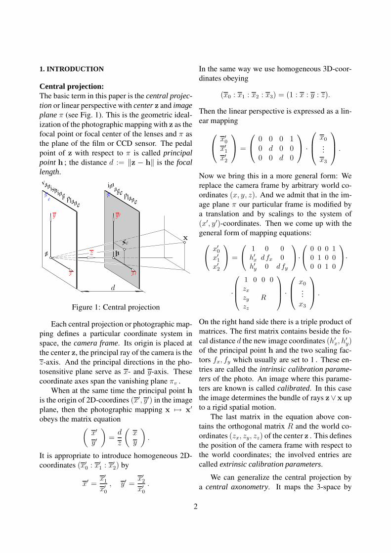
Central projection:The basic term in this paper is the central projec-tion or linear perspective with center z and imageplane π (see Fig. 1). This is the geometric ideal-ization of the photographic mapping with z as thefocal point or focal center of the lenses and π asthe plane of the film or CCD sensor. The pedalpoint of z with respect to π is called principalpoint h ; the distance d := ‖z − h‖ is the focallength.

PSfrag replacements

image plane

vanishing planeππ

v

x

y

z

x

z h

d

xc

x′

y′

Figure 1: Central projection

Each central projection or photographic map-ping defines a particular coordinate system inspace, the camera frame. Its origin is placed atthe center z, the principal ray of the camera is thez-axis. And the principal directions in the pho-tosensitive plane serve as x- and y-axis. Thesecoordinate axes span the vanishing plane πv .

When at the same time the principal point h

is the origin of 2D-coordines (x′, y′) in the imageplane, then the photographic mapping x 7→ x′

obeys the matrix equation(

x′

y′

)=

d

z

(x

y

).

It is appropriate to introduce homogeneous 2D-coordinates (x′

0 : x′

1 : x′

2) by

x′ =x′

1

x′

0

, y′ =x′

2

x′

0

.

In the same way we use homogeneous 3D-coor-dinates obeying

(x0 : x1 : x2 : x3) = (1 : x : y : z).

Then the linear perspective is expressed as a lin-ear mapping

x′

0

x′

1

x′

2

=

0 0 0 10 d 0 00 0 d 0

·

x0

...x3

.

Now we bring this in a more general form: Wereplace the camera frame by arbitrary world co-ordinates (x, y, z). And we admit that in the im-age plane π our particular frame is modified bya translation and by scalings to the system of(x′, y′)-coordinates. Then we come up with thegeneral form of mapping equations:

x′

0

x′

1

x′

2

=

1 0 0h′

x d fx 0h′

y 0 d fy

·

0 0 0 10 1 0 00 0 1 0

·

·

1 0 0 0zx

zy R

zz

·

x0

...x3

.

On the right hand side there is a triple product ofmatrices. The first matrix contains beside the fo-cal distance d the new image coordinates (h′

x, h′

y)of the principal point h and the two scaling fac-tors fx, fy which usually are set to 1 . These en-tries are called the intrinsic calibration parame-ters of the photo. An image where this parame-ters are known is called calibrated. In this casethe image determines the bundle of rays z∨x upto a rigid spatial motion.

The last matrix in the equation above con-tains the orthogonal matrix R and the world co-ordinates (zx, zy, zz) of the center z . This definesthe position of the camera frame with respect tothe world coordinates; the involved entries arecalled extrinsic calibration parameters.

We can generalize the central projection bya central axonometry. It maps the 3-space by

2

a (singular) collinear transformation into the im-age plane. Hence, collinearity of points remainsinvariant and cross ratios are preserved. In ho-mogeneous coordinates a central axonometry canbe expressed by a linear mapping, and there-fore the images are called linear images. Thereare several results on how to characterize per-spective views among linear images (see, e.g.,[6, 13, 7, 11, 2, 12, 8]).

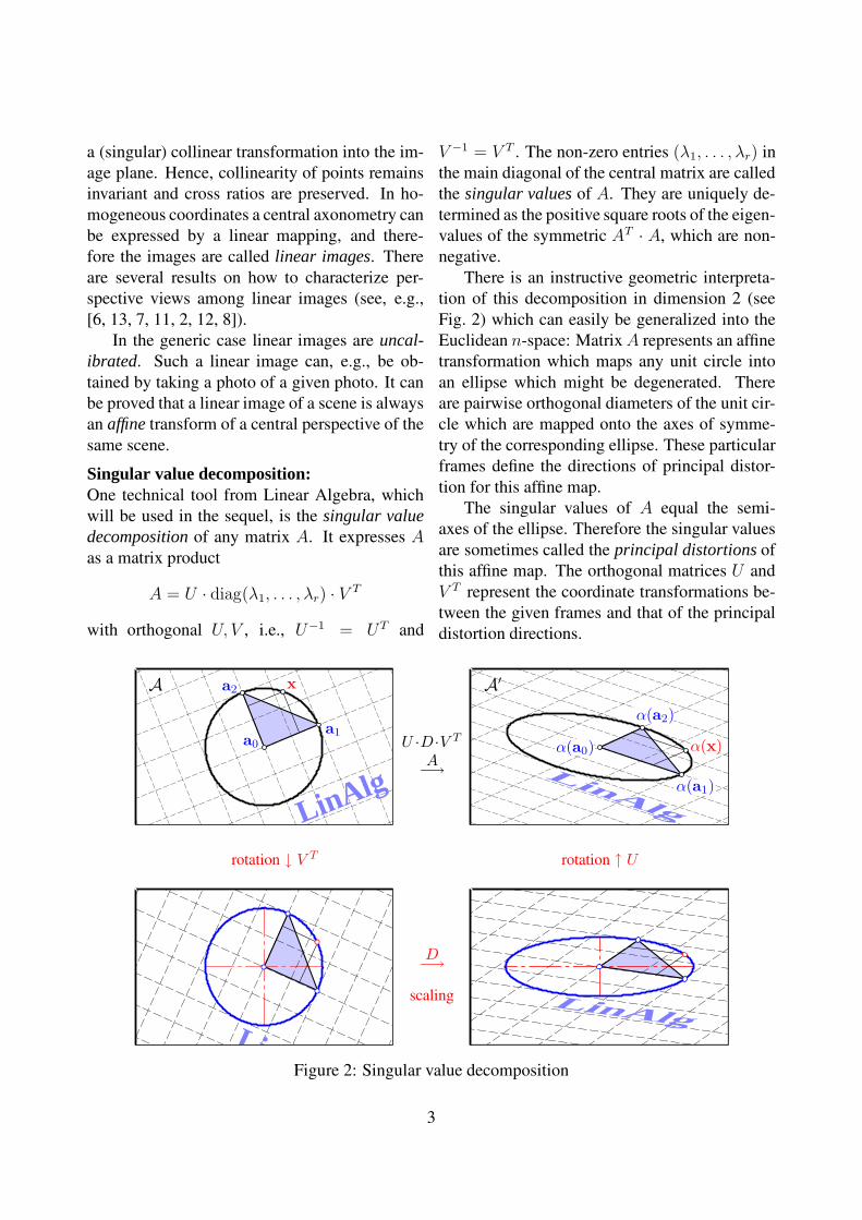
In the generic case linear images are uncal-ibrated. Such a linear image can, e.g., be ob-tained by taking a photo of a given photo. It canbe proved that a linear image of a scene is alwaysan affine transform of a central perspective of thesame scene.Singular value decomposition:One technical tool from Linear Algebra, whichwill be used in the sequel, is the singular valuedecomposition of any matrix A. It expresses A

as a matrix product

A = U · diag(λ1, . . . , λr) · VT

with orthogonal U, V , i.e., U−1 = UT and

LinAlgLinAlg

PSfrag replacements

a0

a1

a2 xA

α(a0)

α(a1)

α(a2)

α(x)

A′

U ·D ·V T

A−→

rotation ↓ V T rotation ↑ U

LinAlg

LinAlg

PSfrag replacementsa0

a1

a2

x

Aα(a0)

α(a1)

α(a2)

α(x)

A′

U ·D ·V T

A−→

a0

a1

a2

x

Aα(a0)

α(a1)

α(a2)

α(x)

A′

D−→

scaling

Figure 2: Singular value decomposition

V −1 = V T . The non-zero entries (λ1, . . . , λr) inthe main diagonal of the central matrix are calledthe singular values of A. They are uniquely de-termined as the positive square roots of the eigen-values of the symmetric AT · A, which are non-negative.

There is an instructive geometric interpreta-tion of this decomposition in dimension 2 (seeFig. 2) which can easily be generalized into theEuclidean n-space: Matrix A represents an affinetransformation which maps any unit circle intoan ellipse which might be degenerated. Thereare pairwise orthogonal diameters of the unit cir-cle which are mapped onto the axes of symme-try of the corresponding ellipse. These particularframes define the directions of principal distor-tion for this affine map.

The singular values of A equal the semi-axes of the ellipse. Therefore the singular valuesare sometimes called the principal distortions ofthis affine map. The orthogonal matrices U andV T represent the coordinate transformations be-tween the given frames and that of the principaldistortion directions.

3

2. THE GEOMETRY OF IMAGE PAIRS

The geometry of pairs of central views has beena classical subject of Descriptive Geometry. Im-portant results are, e.g., due to S. FINSTER-WALDER, E. KRUPPA [9], J. KRAMES, W.WUNDERLICH, H. BRAUNER [1].

π1π1π1π1π1π1π1π1π1π1π1π1π1π1π1π1π1

π2π2π2π2π2π2π2π2π2π2π2π2π2π2π2π2π2

z2z2z2z2z2z2z2z2z2z2z2z2z2z2z2z2z2 z1z1

z1z1z1z1z1z1z1z1z1z1z1z1z1z1z1

z21z21

z21z21

z21z21

z21z21z2

1z21

z21z21z2

1z21

z21z21

z21

z12z12

z12z12

z12z12

z12z12z1

2z12

z12z12z1

2z12

z12z12

z12

zzzzzzzzzzzzzzzzz

x1x1x1x1x1x1x1x1x1x1x1x1x1x1x1x1x1

x2x2x2x2x2x2x2x2x2x2x2x2x2x2x2x2x2

xxxxxxxxxxxxxxxxxδXδXδXδXδXδXδXδXδXδXδXδXδXδXδXδXδX

l1l2l2l2l2l2l2l2l2l2l2l2l2l2l2l2l2l2

π′

1π′

1π′

1π′

1π′

1π′

1π′

1π′

1π′

1π′

1π′

1π′

1π′

1π′

1π′

1π′

1π′

1 π′′

2π′′

2π′′

2π′′

2π′′

2π′′

2π′′

2π′′

2π′′

2π′′

2π′′

2π′′

2π′′

2π′′

2π′′

2π′′

2π′′

2

κ1κ1κ1κ1κ1κ1κ1κ1κ1κ1κ1κ1κ1κ1κ1κ1κ1

κ2κ2κ2κ2κ2κ2κ2κ2κ2κ2κ2κ2κ2κ2κ2κ2κ2

x′x′x′

x′x′

x′x′

x′x′

x′x′

x′x′x′x′x′x′

x′′x′′x′′

x′′x′′

x′′x′′

x′′x′′

x′′x′′

x′′x′′x′′x′′x′′x′′

l′l′l′

l′l′

l′l′

l′l′

l′l′

l′l′l′l′l′l′

l′′l′′l′′

l′′l′′

l′′l′′l′′l′′

l′′l′′l′′l′′l′′l′′l′′l′′

z′2z′2z′

2z′2z′

2z′2z′2z′2z′

2z′2z′2z′2z′

2z′

2z′2z′

2z′2

z′′1z′′1z′′

1z′′1z′′1z′′1z′′1z′′1z′′

1z′′1z′′1z′′1z′′

1z′′

1z′′1z′′

1z′′1

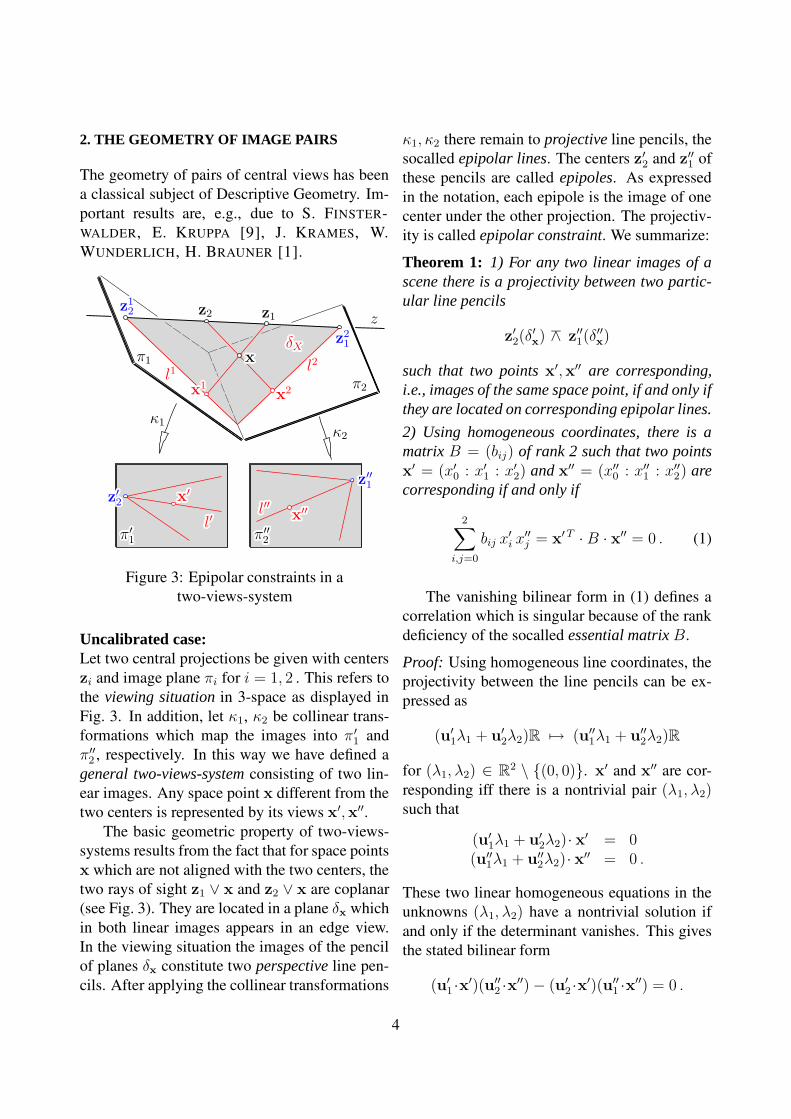
Figure 3: Epipolar constraints in atwo-views-system

Uncalibrated case:Let two central projections be given with centerszi and image plane πi for i = 1, 2 . This refers tothe viewing situation in 3-space as displayed inFig. 3. In addition, let κ1, κ2 be collinear trans-formations which map the images into π ′

1 andπ′′

2 , respectively. In this way we have defined ageneral two-views-system consisting of two lin-ear images. Any space point x different from thetwo centers is represented by its views x′,x′′.

The basic geometric property of two-views-systems results from the fact that for space pointsx which are not aligned with the two centers, thetwo rays of sight z1 ∨ x and z2 ∨ x are coplanar(see Fig. 3). They are located in a plane δ

xwhich

in both linear images appears in an edge view.In the viewing situation the images of the pencilof planes δ

xconstitute two perspective line pen-

cils. After applying the collinear transformations

κ1, κ2 there remain to projective line pencils, thesocalled epipolar lines. The centers z′

2 and z′′1 ofthese pencils are called epipoles. As expressedin the notation, each epipole is the image of onecenter under the other projection. The projectiv-ity is called epipolar constraint. We summarize:Theorem 1: 1) For any two linear images of ascene there is a projectivity between two partic-ular line pencils

z′2(δ′

x) ∧− z′′1(δ

′′

x)

such that two points x′,x′′ are corresponding,i.e., images of the same space point, if and only ifthey are located on corresponding epipolar lines.

2) Using homogeneous coordinates, there is amatrix B = (bij) of rank 2 such that two pointsx′ = (x′

0 : x′

1 : x′

2) and x′′ = (x′′

0 : x′′

1 : x′′

2) arecorresponding if and only if

2∑

i,j=0

bij x′

i x′′

j = x′T · B · x′′ = 0 . (1)

The vanishing bilinear form in (1) defines acorrelation which is singular because of the rankdeficiency of the socalled essential matrix B.Proof: Using homogeneous line coordinates, theprojectivity between the line pencils can be ex-pressed as

(u′

1λ1 + u′

2λ2)R 7→ (u′′

1λ1 + u′′

2λ2)R

for (λ1, λ2) ∈ R2 \ {(0, 0)}. x′ and x′′ are cor-

responding iff there is a nontrivial pair (λ1, λ2)such that

(u′

1λ1 + u′

2λ2)· x′ = 0

(u′′

1λ1 + u′′

2λ2)· x′′ = 0 .

These two linear homogeneous equations in theunknowns (λ1, λ2) have a nontrivial solution ifand only if the determinant vanishes. This givesthe stated bilinear form

(u′

1 ·x′)(u′′

2 ·x′′) − (u′

2 ·x′)(u′′

1 ·x′′) = 0 .

4

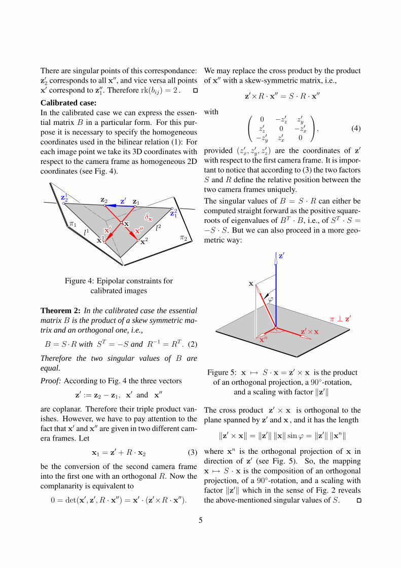
There are singular points of this correspondance:z′2 corresponds to all x′′, and vice versa all pointsx′ correspond to z′′1. Therefore rk(bij) = 2 .Calibrated case:In the calibrated case we can express the essen-tial matrix B in a particular form. For this pur-pose it is necessary to specify the homogeneouscoordinates used in the bilinear relation (1): Foreach image point we take its 3D coordinates withrespect to the camera frame as homogeneous 2Dcoordinates (see Fig. 4).

π1π1π1π1π1π1π1π1π1π1π1π1π1π1π1π1π1

π2π2π2π2π2π2π2π2π2π2π2π2π2π2π2π2π2

z2z2z2z2z2z2z2z2z2z2z2z2z2z2z2z2z2 z1z1

z1z1z1z1z1z1z1z1z1z1z1z1z1z1z1z′z′z

′

z′z′

z′z′z′z′

z′z′z′z′

z′z′z′z′

z21z21

z21z21

z21z21

z21z21z2

1z21

z21z21z2

1z21

z21z21

z21

z12z12

z12z12

z12z12

z12z12z1

2z12

z12z12z1

2z12

z12z12

z12

x1x1x1x1x1x1x1x1x1x1x1x1x1x1x1x1x1

x2x2x2x2x2x2x2x2x2x2x2x2x2x2x2x2x2

xxxxxxxxxxxxxxxxxδx

δxδxδx

δxδx

δxδxδxδx

δxδxδxδx

δxδxδx

l1l2l2l2l2l2l2l2l2l2l2l2l2l2l2l2l2l2x′x′x′

x′x′

x′x′

x′x′

x′x′

x′x′x′x′x′x′

x′′x′′x′′

x′′x′′

x′′x′′

x′′x′′

x′′x′′

x′′x′′x′′x′′x′′x′′

Figure 4: Epipolar constraints forcalibrated images

Theorem 2: In the calibrated case the essentialmatrix B is the product of a skew symmetric ma-trix and an orthogonal one, i.e.,

B = S ·R with ST = −S and R−1 = RT . (2)

Therefore the two singular values of B areequal.

Proof: According to Fig. 4 the three vectors

z′ := z2 − z1, x′ and x′′

are coplanar. Therefore their triple product van-ishes. However, we have to pay attention to thefact that x′ and x′′ are given in two different cam-era frames. Let

x1 = z′ + R · x2 (3)

be the conversion of the second camera frameinto the first one with an orthogonal R. Now thecomplanarity is equivalent to

0 = det(x′, z′, R · x′′) = x′ · (z′×R · x′′).

We may replace the cross product by the productof x′′ with a skew-symmetric matrix, i.e.,

z′×R · x′′ = S · R · x′′

with

0 −z′z z′yz′z 0 −z′x−z′y z′x 0

, (4)

provided (z′x, z′

y, z′

z) are the coordinates of z′

with respect to the first camera frame. It is impor-tant to notice that according to (3) the two factorsS and R define the relative position between thetwo camera frames uniquely.The singular values of B = S · R can either becomputed straight forward as the positive square-roots of eigenvalues of BT · B, i.e., of ST · S =−S · S. But we can also proceed in a more geo-metric way:

PSfrag replacements z′

x

xnz′×x

ϕ

π ⊥ z′

Figure 5: x 7→ S · x = z′ × x is the productof an orthogonal projection, a 90◦-rotation,

and a scaling with factor ‖z′‖

The cross product z′ × x is orthogonal to theplane spanned by z′ and x , and it has the length

‖z′ × x‖ = ‖z′‖ ‖x‖ sinϕ = ‖z′‖ ‖xn‖

where xn is the orthogonal projection of x indirection of z′ (see Fig. 5). So, the mappingx 7→ S · x is the composition of an orthogonalprojection, of a 90◦-rotation, and a scaling withfactor ‖z′‖ which in the sense of Fig. 2 revealsthe above-mentioned singular values of S.

5

3. THE FUNDAMENTAL THEOREMS

What means ‘reconstruction’ from two images ?The photos have been taken in a particular view-ing situation. But afterwards we have only thetwo images, and we know nothing about howthe camera frames where mutually placed in 3-space. Hence, reconstruction means both, recov-ering the viewing situation and recovering the de-picted scene.

The problem of recovering a scene from twoor more images is a basic problem in ComputerVision (see, e.g., [3, 4, 15, 5]). It is remark-able, that sometimes in the cited books the au-thors really refer to results which have alreadybeen achieved in Descriptive Geometry (note,e.g., the high estimation of E. KRUPPA’s results[9] in [15]). However, Computer Vision focuseson numerical solutions, and the use of computersbrought new insight and progress in this prob-lem. Since measuring pixels in any image can becarried out with standard software, it has becomepossible to recover an object with high precisionfrom two digital images just by using a laptop.Theorem 3: From two uncalibrated imageswith given projectivity between epipolar linesthe depicted object can be reconstructed up to acollinear transformation.

Sketch of the proof: The two images can beplaced in space such that pairs of epipolar linesare intersecting:

For this purpose we start with a positionwhere the two images are coplanar and two cor-responding lines are aligned. Then the two pen-cils of epipolar lines are perspective with respectto an axis a . Now we rotate one of the im-age planes about this axis a . The correspondingepipolar lines are still intersecting on a . Then wespecify arbitrary centers z1, z2 on the baseline z

which connects the two epipoles. This gives riseto a reconstructed 3D object.

Any other choice of the viewing situationgives a collinear transform of the previously re-covered 3D object.

Theorem 4: (S. Finsterwalder, 1899)From two calibrated images with given projectiv-ity between epipolar lines the depicted object canbe reconstructed up to a similarity.

Sketch of the proof: In the corresponding bun-dles of rays the pencils of epipolar planes δ

xfor

both projections need to be congruent. There isa rigid motion of one camera frame such thatany two corresponding epipolar planes are co-incident. For any choice of z2 relative to z1 onthe carrier line z of the unified pencil of planesthere exists a reconstructed 3D object. Any otherchoice of z2 gives a similar 3D object.

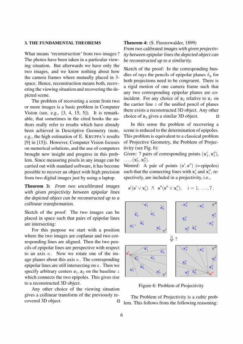
In this sense the problem of recovering ascene is reduced to the determination of epipoles.This problem is equivalent to a classical problemof Projective Geometry, the Problem of Projec-tivity (see Fig. 6):Given: 7 pairs of corresponding points (x′

1,x′′

1),. . . , (x′

7,x′′

7).Wanted: A pair of points (s′, s′′) (= epipoles)such that the connecting lines with x′

i and x′′

i , re-spectively, are included in a projectivity, i.e.,

s′(s′ ∨ x′

i) ∧− s′′(s′′ ∨ x′′

i ), i = 1, . . . , 7 .

PSfrag replacements

x′

1x

′

2

x′

3x′

4

x′

5

x′

6x

′

7

x′′

1

x′′

2

x′′

3x

′′

4

x′′

5

x′′

6x′′

7

s′

s′′

π′

π′′

⇓ ?

PSfrag replacements

x′

1x

′

2

x′

3x′

4

x′

5

x′

6x

′

7

x′′

1

x′′

2

x′′

3x

′′

4

x′′

5

x′′

6x′′

7

s′

s′′π′

π′′

Figure 6: Problem of Projectivity

The Problem of Projectivity is a cubic prob-lem. This follows from the following reasoning:

6

Due to (1) the 7 given pairs of correspondingpoints give 7 linear homogeneous equations

xTi · B · x′′

i = 0, i = 1, . . . , 7 , (5)

for the 9 entries in the essential (3× 3)-matrixB = (bij). The condition rk(B) = 2 gives theadditional cubic equation det B = 0 which fixesall bij up to a common factor.

4. COMPUTING THE ESSENTIAL MATRIX

For noisy image points it is recommended to usemore than 7 points and to apply methods of leastsquares approximation for obtaining the ‘best fit-ting’ matrix B :

Let A denote the coefficient matrix in the lin-ear system (5) of homogeneous equations for theentries of B. Then the ‘least square fit’ B isan eigenvector for the smallest eigenvalue of thesymmetric matrix AT · A which minimizes

yT · AT · A · y = ‖A · y‖2

under the side condition ‖y‖ = 1 .Any essential matrix has the rank 2, and in

particular in the calibrated case the two singularvalues must be equal. In order to obtain such a‘best fitting’ essential matrix B for our obtainedB, we use what sometimes is called the ’projec-tion into the essential space’:

This is based on the singular value decom-position of B, which has been presented in Sec-tion 1. It factorizes B as a matrix product

B = U · D · V T , D = diag(λ1, λ2, λ3),

with orthogonal U, V . For the singular values ofB we suppose λ1 ≥ λ2 ≥ λ3 .

Then in the uncalibrated case the best fittingessential matrix reads

B = U · diag(λ1, λ2, 0) · V T . (6)

In the calibrated case

B = U ·diag(λ, λ, 0)·V T with λ =λ1+λ2

2(7)

is optimal in the sense of the Frobenius norm‖A‖f for square matrices A (see, e.g., [10, 15]).‖A‖2

f equals the trace of AT ·A and therefore thesquare sum of the singular values of A.

In the uncalibrated case the solution B of (6)gives

‖B − B‖f = λ3

which is minimal among all rank 2 matrices. Inthe calibrated case the solution B presented in (7)yields the error

‖B − B‖f =√

(λ − λ1)2 + (λ − λ2)2 + λ23 ,

which is minimal among all possible essentialmatrices.

The factorization B = S · R according toTheorem 2 reveals already the relative positionof the two camera frames. Therefore we need

Theorem 5: The factorization of the essentialmatrix B = U · D · V T , D = diag(λ, λ, 0), intothe skew symmetric matrix S and the orthogonalmatrix R reads:

S = ±U · R+ · D · UT , R = ±U · RT+ · V T

where R+ =

0 −1 01 0 00 0 1

. (8)

Proof: It is sufficient to factorize the product ofthe first two matrices by

U · D = S · R′,

because this implies immediately

B = S · (R′ · V T ), i.e., R = R′ · V T .

We focus on the affine 3D transformations whichare represented by the involved matrices:• U ·D is composed from the orthogonal projec-tion parallel to the z-axis, the scaling with factorλ and the rotation U which transforms the z-axisinto the kernel of U · B.• On the other hand, the skew symmetric matrixS represents the orthogonal projection parallel z′

composed with a 90◦-rotation about z′ and a scal-ing with factor ‖z′‖ (see Fig. 5).

7

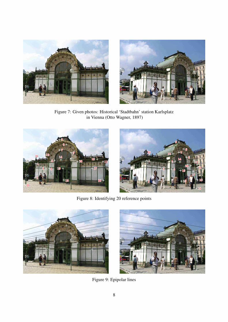
Figure 7: Given photos: Historical ‘Stadtbahn’ station Karlsplatzin Vienna (Otto Wagner, 1897)

11111111111111111

22222222222222222

33333333333333333 44444444444444444

55555555555555555

6666666666666666677777777777777777

88888888888888888

99999999999999999

1010101010101010101010101010101010

1111111111111111111111111111111111

1212121212121212121212121212121212

13131313131313131313131313131313131414141414141414141414141414141414

1515151515151515151515151515151515

1616161616161616161616161616161616

1717171717171717171717171717171717

1818181818181818181818181818181818

1919191919191919191919191919191919

2020202020202020202020202020202020 11111111111111111

22222222222222222

33333333333333333 44444444444444444

55555555555555555

66666666666666666

77777777777777777

88888888888888888

99999999999999999

1010101010101010101010101010101010

1111111111111111111111111111111111

1212121212121212121212121212121212

1313131313131313131313131313131313

1414141414141414141414141414141414

1515151515151515151515151515151515

1616161616161616161616161616161616

1717171717171717171717171717171717

1818181818181818181818181818181818

1919191919191919191919191919191919

2020202020202020202020202020202020

Figure 8: Identifying 20 reference points

Figure 9: Epipolar lines

8

Let R+ denote the matrix representing the90◦-rotation about the z-axis. Then R+ is of theform stated in Theorem 5. The product R+ ·D =D ·R+ is skew-symmetric and thus we obtain thefollowing two solutions:

S = ±U · R+ · D · UT and R′ = ±U · RT+ .

For the following reason, these are the only twopossible factorizations of the required type:As matrix B represents an orthogonal axonom-etry, the column vectors are the images of anorthonormal frame. We know from DescriptiveGeometry that apart from translations parallel tothe rays of sight there are exactly two differenttriples of pairwise orthogonal axes with imagesin direction of the given column vectors. The twotriples are mirror images from each other. So, wecan’t expect more than two factorizations.

There are critical configurations where thespecified reference points are not sufficient todetermine the epipoles uniquely. This is, e.g.,the case when only coplanar 3D points are cho-sen as reference points. But there are also othercases related to quadrics. For details see, e.g.,[14, 15, 5]).

5. THE ALGORITHM

We summarize: The numerical reconstruction oftwo calibrated images with the aid of any com-puter algebra system (e.g., Maple) consists of thefollowing five steps:

1) Specify n > 7 pairs (x′

i,x′′

i ), i = 1, . . . , n,of corresponding points under avoidanceof critical configurations.

2) Set up the homogeneous linear system ofequations x′T

i ·B ·x′′

i = 0 for the unknownfundamental matrix B. The optimal so-lution B is an eigenvector of the smallesteigenvalue of AT · A with A as the coeffi-cient matrix of this system.

PSfrag replacements

1

2

3 4

5

6

7

8

9

9

10

11

12

12

13

1314

15

16

17

18

19

20

z1

z1

z2

z2

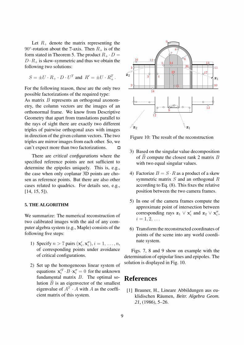
Figure 10: The result of the reconstruction

3) Based on the singular value decompositionof B compute the closest rank 2 matrix B

with two equal singular values.

4) Factorize B = S ·R as a product of a skewsymmetric matrix S and an orthogonal R

according to Eq. (8). This fixes the relativeposition between the two camera frames.

5) In one of the camera frames compute theapproximate point of intersection betweencorresponding rays z1 ∨ x′

i and z2 ∨ x′′

i ,i = 1, 2, . . .

6) Transform the reconstructed coordinates ofpoints of the scene into any world coordi-nate system.

Figs. 7, 8 and 9 show on example with thedetermination of epipolar lines and epipoles. Thesolution is displayed in Fig. 10.

References

[1] Brauner, H., Lineare Abbildungen aus eu-klidischen Raumen, Beitr. Algebra Geom.21, (1986), 5–26.

9

[2] Dur, A., An Algebraic Equation for theCentral Projection, J. Geometry Graphics7, (2003), 137–143.

[3] Faugeras, O., Three-Dimensional Com-puter Vision. A Geometric Viewpoint, MITPress, Cambridge, Mass., 1996.

[4] Faugeras, O., and Q.-T. Luong, The Geom-etry of Multiple Images, MIT Press, Cam-bridge, Mass., 2001.

[5] Hartley, R., and Zisserman, A., MultipleView Geometry in Computer Vision. Cam-bridge University Press, 2000.

[6] Havel, V., O rozkladu singularnıch linear-nıch transformacı, Casopis Pest. Mat. 85,(1960), 439–447.

[7] Havlicek, H., On the Matrices of Cen-tral Linear Mappings, Math. Bohem. 121,(1996), 151–156.

[8] Hoffmann, M., and Yiu, P., Moving CentralAxonometric Reference Systems, J. Geom-etry Graphics 9, (2005), 133–140.

[9] Kruppa, E., Zur achsonometrischen Meth-ode der darstellenden Geometrie, Sitzungs-ber., Abt. II, osterr. Akad. Wiss., Math.-Naturw. Kl. 119, (1910), 487–506.

[10] Lawson, C.L., and Hanson, R.J., SolvingLeast Squares Problems, siam, 1995, 1sted.: Prentice-Hall, Inc., Englewood Cliffs,NJ, 1974.

[11] Stachel, H., Zur Kennzeichnung derZentralprojektionen nach H. Havlicek,Sitzungsber., Abt. II, osterr. Akad. Wiss.,Math.-Naturw. Kl. 204, (1995), 33–46.

[12] Stachel, H., On Arne Dur’s Equation Con-cerning Central Axonometries, J. GeometryGraphics 8, (2004), 215–224.

[13] Szabo, J., Stachel, H. and Vogel, H., EinSatz uber die Zentralaxonometrie, Sitzungs-ber., Abt. II, osterr. Akad. Wiss., Math.-Naturw. Kl. 203, (1994), 3–11.

[14] Tschupik, J., and Hohenberg, F., Die geo-metrische Grundlagen der Photogramme-trie, in Jordan, Eggert, Kneissl (eds.):Handbuch der Vermessungskunde III a/3,10. Aufl., Metzlersche Verlagsbuchhand-lung, Stuttart 1972, 2235–2295.

[15] Yi Ma, Soatto, St., Kosecka, J., and Sas-try, S. Sh., An Invitation to 3-D Vision.Springer-Verlag, New York 2004.

ABOUT THE AUTHOR

Hellmuth Stachel, Ph.D, is Professor of Ge-ometry at the Institute of Discrete Mathemat-ics and Geometry, Vienna University of Tech-nology, and editor in chief of the “Journal forGeometry and Graphics”. His research interestsare in Higher Geometry, Kinematics and Com-puter Graphics. He can be reached by e-mail:stachel@dmg.tuwien.ac.at, by fax: (+431)-58801-11399, or through the postal address:Institut fur Diskrete Mathematik und Geometrie /Technische Universitat Wien / Wiedner Hauptstr.8-10/104 / A 1040 Wien / Austria, Europe.

10