descriptions of the algorithms - sourceforgepragmath.sourceforge.net/algorithms.pdf · descriptions...
TRANSCRIPT
Descriptions of the Algorithmswith several illustrations by the author
Christoph Zurnieden�[email protected] �
Last change: July 29, 2008
-6
-4
-2
0
2
4
6
-6 -4 -2 0 2 4 6
Contents
����������� ����� 9
Introduction 10
1 Special Data Types 121.1 Matrix . . . . . . . . . . . . . . . . . . . . . . . . . . . . . . . . . 12
1.1.1 Usage of the Class . . . . . . . . . . . . . . . . . . . . . . 121.2 Complex . . . . . . . . . . . . . . . . . . . . . . . . . . . . . . . . 14
1.2.1 � . . . . . . . . . . . . . . . . . . . . . . . . . . . . . . . . . 141.2.2 Usage of the Class . . . . . . . . . . . . . . . . . . . . . . 15
1.3 Vector . . . . . . . . . . . . . . . . . . . . . . . . . . . . . . . . . . 15
2 Constants 162.1 Mathematical Constants . . . . . . . . . . . . . . . . . . . . . . . 16
2.1.1 Airy functions . . . . . . . . . . . . . . . . . . . . . . . . . 162.1.2 Apery’s Constant ( ������� ) . . . . . . . . . . . . . . . . . . . 172.1.3 �����! #"$ . . . . . . . . . . . . . . . . . . . . . . . . . . . . . . 172.1.4 Artins Constant . . . . . . . . . . . . . . . . . . . . . . . . 182.1.5 Backhouse’s Constant . . . . . . . . . . . . . . . . . . . . 182.1.6 Bernstein’s Constant . . . . . . . . . . . . . . . . . . . . . 182.1.7 Brun’s Constant . . . . . . . . . . . . . . . . . . . . . . . . 192.1.8 Cahen’s Constant . . . . . . . . . . . . . . . . . . . . . . . 192.1.9 Catalan’s Constant . . . . . . . . . . . . . . . . . . . . . . 192.1.10 Champernown’s constant . . . . . . . . . . . . . . . . . . 202.1.11 Continued Fraction Constant . . . . . . . . . . . . . . . . 202.1.12 Conway’s Constant . . . . . . . . . . . . . . . . . . . . . . 202.1.13 Copeland-Erdos’ Constant . . . . . . . . . . . . . . . . . . 212.1.14 %�&('*) . . . . . . . . . . . . . . . . . . . . . . . . . . . . . . 212.1.15 %�&('�+,) . . . . . . . . . . . . . . . . . . . . . . . . . . . . . . 212.1.16 -. / . . . . . . . . . . . . . . . . . . . . . . . . . . . . . . . 212.1.17 -. � . . . . . . . . . . . . . . . . . . . . . . . . . . . . . . . 222.1.18 Dubois-Raymond Constant . . . . . . . . . . . . . . . . . 222.1.19 Euler-Mascheroni Constant � . . . . . . . . . . . . . . . . 222.1.20 Embree-Trefethen Constant . . . . . . . . . . . . . . . . . 22
2
Contents Contents
2.1.21 Erdos-Borwein Constant . . . . . . . . . . . . . . . . . . . 232.1.22 0 . . . . . . . . . . . . . . . . . . . . . . . . . . . . . . . . . 232.1.23 Gompertz’ constant . . . . . . . . . . . . . . . . . . . . . 232.1.24 Feigenbaum Constants . . . . . . . . . . . . . . . . . . . . 242.1.25 Fibonacci Factorial Constant . . . . . . . . . . . . . . . . 272.1.26 Fransen-Robinson Constant . . . . . . . . . . . . . . . . . 272.1.27 Froda’s Constant . . . . . . . . . . . . . . . . . . . . . . . 272.1.28 Gibbs Constant 12��� � � . . . . . . . . . . . . . . . . . . . . . 272.1.29 Gauss-Kuzmin-Wirsing Constant . . . . . . . . . . . . . . 282.1.30 Glaisher-Kinkelin Constant . . . . . . . . . . . . . . . . . 282.1.31 Golden Ratio . . . . . . . . . . . . . . . . . . . . . . . . . 282.1.32 Golomb’s Constant . . . . . . . . . . . . . . . . . . . . . . 302.1.33 Grothendieck’s Majorant . . . . . . . . . . . . . . . . . . 302.1.34 Hadamard-de la Valle-Poussin Constant . . . . . . . . . 302.1.35 Hafner-Sarnak-McCurley Constant . . . . . . . . . . . . . 312.1.36 Hard-Hexagon Entropy Constant . . . . . . . . . . . . . 312.1.37 Khintchine Constant . . . . . . . . . . . . . . . . . . . . . 332.1.38 Khintchine’s Harmonic Mean . . . . . . . . . . . . . . . . 342.1.39 Komornik-Loreti Constant . . . . . . . . . . . . . . . . . . 342.1.40 Second Order Landau-Ramanujan Constant . . . . . . . 352.1.41 Laplace Limit Constant . . . . . . . . . . . . . . . . . . . 362.1.42 Lehmer Constant . . . . . . . . . . . . . . . . . . . . . . . 362.1.43 Lemniscate Constant . . . . . . . . . . . . . . . . . . . . . 362.1.44 Lengyel Constant . . . . . . . . . . . . . . . . . . . . . . . 372.1.45 Levy constant . . . . . . . . . . . . . . . . . . . . . . . . . 372.1.46 Madelung’s Constant . . . . . . . . . . . . . . . . . . . . 372.1.47 Magata’s constant . . . . . . . . . . . . . . . . . . . . . . 382.1.48 Meissel-Mertens constant . . . . . . . . . . . . . . . . . . 382.1.49 Niven’s constant . . . . . . . . . . . . . . . . . . . . . . . 382.1.50 Reciprocal of the One-Ninth-Constant . . . . . . . . . . . 392.1.51 One-Ninth-Constant . . . . . . . . . . . . . . . . . . . . . 392.1.52 Paris Constant . . . . . . . . . . . . . . . . . . . . . . . . . 402.1.53 Parking Renyi Constant . . . . . . . . . . . . . . . . . . . 402.1.54 Smallest Pisot-Vijayaraghavan Number . . . . . . . . . . 412.1.55 Plastic Constant . . . . . . . . . . . . . . . . . . . . . . . . 422.1.56 Porter constant . . . . . . . . . . . . . . . . . . . . . . . . 422.1.57 Sum of the Product of the Inverse of Primes . . . . . . . 422.1.58 Rabbit Constant . . . . . . . . . . . . . . . . . . . . . . . . 432.1.59 Ramanujan-Soldner Constant . . . . . . . . . . . . . . . . 442.1.60 Reciprocal Fibonacci Constant . . . . . . . . . . . . . . . 442.1.61 Reciprocal Prime Constant . . . . . . . . . . . . . . . . . 442.1.62 Robbins’ Constant . . . . . . . . . . . . . . . . . . . . . . 442.1.63 Smallest Known Salem Number . . . . . . . . . . . . . . 452.1.64 Sierpinski Constant . . . . . . . . . . . . . . . . . . . . . . 452.1.65 '435 6) . . . . . . . . . . . . . . . . . . . . . . . . . . . . . . . 452.1.66 '435 7+6) . . . . . . . . . . . . . . . . . . . . . . . . . . . . . . 45
PRAGMATIC MATHEMATICAL SERVICE 3
Contents Contents
2.1.67 Traveling Salesman Constant . . . . . . . . . . . . . . . . 452.1.68 Tribonacci Constant . . . . . . . . . . . . . . . . . . . . . 462.1.69 Gauss constant . . . . . . . . . . . . . . . . . . . . . . . . 462.1.70 Universal Parabolic Constant . . . . . . . . . . . . . . . . 472.1.71 Viswanath’s Constant . . . . . . . . . . . . . . . . . . . . 472.1.72 Weierstrass Constant . . . . . . . . . . . . . . . . . . . . . 482.1.73 Some � Values . . . . . . . . . . . . . . . . . . . . . . . . . 48
2.2 Physical Constants . . . . . . . . . . . . . . . . . . . . . . . . . . 482.2.1 Astronomical Unit . . . . . . . . . . . . . . . . . . . . . . 482.2.2 Avogadro Constant . . . . . . . . . . . . . . . . . . . . . . 482.2.3 Boltzmann Constant . . . . . . . . . . . . . . . . . . . . . 482.2.4 Candela . . . . . . . . . . . . . . . . . . . . . . . . . . . . 492.2.5 Dielectric Constants . . . . . . . . . . . . . . . . . . . . . 492.2.6 Dirac Constant . . . . . . . . . . . . . . . . . . . . . . . . 492.2.7 Gas Constant . . . . . . . . . . . . . . . . . . . . . . . . . 492.2.8 Weight of One Mol Water . . . . . . . . . . . . . . . . . . 492.2.9 Speed of Light . . . . . . . . . . . . . . . . . . . . . . . . . 492.2.10 Light Year . . . . . . . . . . . . . . . . . . . . . . . . . . . 502.2.11 Magnetic Permeability of the Vacuum . . . . . . . . . . . 502.2.12 Newton’s Gravity Constant . . . . . . . . . . . . . . . . . 502.2.13 Parsec . . . . . . . . . . . . . . . . . . . . . . . . . . . . . 502.2.14 Planck Constant . . . . . . . . . . . . . . . . . . . . . . . . 512.2.15 Seconds in a Year . . . . . . . . . . . . . . . . . . . . . . . 512.2.16 Stefan-Boltzmann constant . . . . . . . . . . . . . . . . . 512.2.17 Luminosity of the Sun . . . . . . . . . . . . . . . . . . . . 512.2.18 Electric Constant . . . . . . . . . . . . . . . . . . . . . . . 512.2.19 Wien’s displacement constant . . . . . . . . . . . . . . . . 51
3 Common Functions 523.1 Basic operations . . . . . . . . . . . . . . . . . . . . . . . . . . . . 52
3.1.1 Operations on complex numbers . . . . . . . . . . . . . . 523.1.2 Operations on Matrices . . . . . . . . . . . . . . . . . . . 56
3.2 Geometric Functions . . . . . . . . . . . . . . . . . . . . . . . . . 603.2.1 Triangle . . . . . . . . . . . . . . . . . . . . . . . . . . . . 603.2.2 Polygon . . . . . . . . . . . . . . . . . . . . . . . . . . . . 613.2.3 Circle . . . . . . . . . . . . . . . . . . . . . . . . . . . . . . 633.2.4 Ellipse . . . . . . . . . . . . . . . . . . . . . . . . . . . . . 653.2.5 Sphere . . . . . . . . . . . . . . . . . . . . . . . . . . . . . 663.2.6 Torus . . . . . . . . . . . . . . . . . . . . . . . . . . . . . . 673.2.7 Cone . . . . . . . . . . . . . . . . . . . . . . . . . . . . . . 673.2.8 Miscellaneous Geometric Figures . . . . . . . . . . . . . . 68
3.3 Trigonometric Functions . . . . . . . . . . . . . . . . . . . . . . . 703.3.1 Complex.prototype.sin . . . . . . . . . . . . . . . . 703.3.2 Complex.prototype.cos . . . . . . . . . . . . . . . . 703.3.3 Complex.prototype.tan . . . . . . . . . . . . . . . . 703.3.4 Complex.prototype.asin . . . . . . . . . . . . . . . . 70
4 PRAGMATIC MATHEMATICAL SERVICE

Contents Contents
3.3.5 Complex.prototype.acos . . . . . . . . . . . . . . . . 703.3.6 Complex.prototype.atan . . . . . . . . . . . . . . . . 713.3.7 Math.cot . . . . . . . . . . . . . . . . . . . . . . . . . . . 713.3.8 Complex.prototype.cot . . . . . . . . . . . . . . . . 713.3.9 Math.acot . . . . . . . . . . . . . . . . . . . . . . . . . . 713.3.10 Complex.prototype.acot . . . . . . . . . . . . . . . . 713.3.11 Complex.prototype.acoth . . . . . . . . . . . . . . . 713.3.12 Math.sec . . . . . . . . . . . . . . . . . . . . . . . . . . . 713.3.13 Complex.prototype.sec . . . . . . . . . . . . . . . . 723.3.14 Complex.prototype.sech . . . . . . . . . . . . . . . . 723.3.15 Complex.prototype.asec . . . . . . . . . . . . . . . . 723.3.16 Complex.prototype.asech . . . . . . . . . . . . . . . 723.3.17 Math.csc and Math.cosec . . . . . . . . . . . . . . . . 723.3.18 Complex.prototype.csc . . . . . . . . . . . . . . . . 723.3.19 Complex.prototype.csch . . . . . . . . . . . . . . . . 723.3.20 Complex.prototype.acsc . . . . . . . . . . . . . . . . 733.3.21 Complex.prototype.acsch . . . . . . . . . . . . . . . 733.3.22 Math.sem . . . . . . . . . . . . . . . . . . . . . . . . . . . 733.3.23 Math.asem . . . . . . . . . . . . . . . . . . . . . . . . . . 733.3.24 Math.atan2 . . . . . . . . . . . . . . . . . . . . . . . . . 733.3.25 Math.cosh . . . . . . . . . . . . . . . . . . . . . . . . . . 733.3.26 Math.sinh . . . . . . . . . . . . . . . . . . . . . . . . . . 743.3.27 Math.tanh . . . . . . . . . . . . . . . . . . . . . . . . . . 743.3.28 Complex.prototype.tanh . . . . . . . . . . . . . . . . 743.3.29 Math.coth . . . . . . . . . . . . . . . . . . . . . . . . . . 743.3.30 Complex.prototype.coth . . . . . . . . . . . . . . . . 743.3.31 Math.acosh . . . . . . . . . . . . . . . . . . . . . . . . . 743.3.32 Complex.prototype.acosh . . . . . . . . . . . . . . . 753.3.33 Math.asinh . . . . . . . . . . . . . . . . . . . . . . . . . 753.3.34 Complex.prototype.asinh . . . . . . . . . . . . . . . 753.3.35 Math.atanh . . . . . . . . . . . . . . . . . . . . . . . . . 753.3.36 Complex.prototype.atanh . . . . . . . . . . . . . . . 753.3.37 Math.acoth . . . . . . . . . . . . . . . . . . . . . . . . . 753.3.38 Conversions . . . . . . . . . . . . . . . . . . . . . . . . . . 76
4 Special Functions 784.1 Dilogarithm . . . . . . . . . . . . . . . . . . . . . . . . . . . . . . 784.2 Exponential Integral . . . . . . . . . . . . . . . . . . . . . . . . . 784.3 Kummer’s Confluent Hypergeometric Function . . . . . . . . . 784.4 Fresnel Integrals . . . . . . . . . . . . . . . . . . . . . . . . . . . . 784.5 Bessel Functions . . . . . . . . . . . . . . . . . . . . . . . . . . . . 80
4.5.1 Differential Equation . . . . . . . . . . . . . . . . . . . . . 814.5.2 Ascending Series . . . . . . . . . . . . . . . . . . . . . . . 824.5.3 Relation to the Gamma-function . . . . . . . . . . . . . . 824.5.4 Wronskians . . . . . . . . . . . . . . . . . . . . . . . . . . 824.5.5 Asymptotic Expansions for Large Arguments . . . . . . 83
PRAGMATIC MATHEMATICAL SERVICE 5
Contents Contents
4.6 Beta Functions . . . . . . . . . . . . . . . . . . . . . . . . . . . . . 854.6.1 Beta function 8,��9�:�;<� . . . . . . . . . . . . . . . . . . . . . 854.6.2 Incomplete Beta Function . . . . . . . . . . . . . . . . . . 854.6.3 Regularized Incomplete Beta Function . . . . . . . . . . . 86
4.7 Gamma Functions . . . . . . . . . . . . . . . . . . . . . . . . . . . 864.7.1 = -function . . . . . . . . . . . . . . . . . . . . . . . . . . . 864.7.2 Incomplete = -function . . . . . . . . . . . . . . . . . . . . 894.7.3 Regularized = -function . . . . . . . . . . . . . . . . . . . 894.7.4 Digamma >@?(��A�� or B . . . . . . . . . . . . . . . . . . . . . 894.7.5 Polygamma >@C���A�� . . . . . . . . . . . . . . . . . . . . . . 914.7.6 Double Factorial . . . . . . . . . . . . . . . . . . . . . . . 914.7.7 Hyperfactorial . . . . . . . . . . . . . . . . . . . . . . . . . 914.7.8 Raising Factorial (Pochhammer Symbol) . . . . . . . . . 914.7.9 K-Function . . . . . . . . . . . . . . . . . . . . . . . . . . . 924.7.10 Barne’s G-Function . . . . . . . . . . . . . . . . . . . . . . 92
4.8 Error Function . . . . . . . . . . . . . . . . . . . . . . . . . . . . . 924.9 Generalized Laguerre Function . . . . . . . . . . . . . . . . . . . 944.10 � (Riemann, Hurwitz), DFEC . . . . . . . . . . . . . . . . . . . . . . 94
4.10.1 Riemann’s � -Function . . . . . . . . . . . . . . . . . . . . 944.10.2 Hurwitz’ � -Function . . . . . . . . . . . . . . . . . . . . . 954.10.3 General Partial Harmonic Function DGEC . . . . . . . . . . 954.10.4 Partial Harmonic Function D "C . . . . . . . . . . . . . . . 95
5 Linear Algebra (Matrices) 975.1 Matrix Decompositions . . . . . . . . . . . . . . . . . . . . . . . . 97
5.1.1 Eigen Decomposition . . . . . . . . . . . . . . . . . . . . 975.1.2 LU Decomposition . . . . . . . . . . . . . . . . . . . . . . 975.1.3 QR Decomposition . . . . . . . . . . . . . . . . . . . . . . 975.1.4 Singular Value Decomposition . . . . . . . . . . . . . . . 97
5.2 Systems of Equations . . . . . . . . . . . . . . . . . . . . . . . . . 975.2.1 Determinant . . . . . . . . . . . . . . . . . . . . . . . . . . 97
6 Sets 986.1 Equality HJILK . . . . . . . . . . . . . . . . . . . . . . . . . . . . 986.2 Union HNMOK . . . . . . . . . . . . . . . . . . . . . . . . . . . . . . 986.3 Intersection HNPOK . . . . . . . . . . . . . . . . . . . . . . . . . . 996.4 Difference HRQSK . . . . . . . . . . . . . . . . . . . . . . . . . . . . 99
6.4.1 Absolute Complement . . . . . . . . . . . . . . . . . . . . 996.4.2 Relative Complement . . . . . . . . . . . . . . . . . . . . 1006.4.3 Symmetric Difference . . . . . . . . . . . . . . . . . . . . 101
6.5 Power . . . . . . . . . . . . . . . . . . . . . . . . . . . . . . . . . . 1026.5.1 Families and other Collections . . . . . . . . . . . . . . . 102
6.6 Cartesian Product HUTVK . . . . . . . . . . . . . . . . . . . . . . . 1026.6.1 Binary Relation . . . . . . . . . . . . . . . . . . . . . . . . 103
7 Combinatorics 106
6 PRAGMATIC MATHEMATICAL SERVICE

Contents Contents
8 Statistical Functions 1078.1 Distributions . . . . . . . . . . . . . . . . . . . . . . . . . . . . . . 107
8.1.1 Beta Distribution . . . . . . . . . . . . . . . . . . . . . . . 1078.1.2 Binomial . . . . . . . . . . . . . . . . . . . . . . . . . . . . 1088.1.3 Cauchy . . . . . . . . . . . . . . . . . . . . . . . . . . . . . 1088.1.4 F-Distribution . . . . . . . . . . . . . . . . . . . . . . . . . 1098.1.5 Geometric . . . . . . . . . . . . . . . . . . . . . . . . . . . 1098.1.6 Hypergeometric . . . . . . . . . . . . . . . . . . . . . . . . 110
8.2 Means . . . . . . . . . . . . . . . . . . . . . . . . . . . . . . . . . . 1118.2.1 Range . . . . . . . . . . . . . . . . . . . . . . . . . . . . . 1118.2.2 Harmonic Mean . . . . . . . . . . . . . . . . . . . . . . . . 1118.2.3 Geometric Mean . . . . . . . . . . . . . . . . . . . . . . . 1118.2.4 Root-Mean-Square . . . . . . . . . . . . . . . . . . . . . . 1128.2.5 Arithmetic Mean . . . . . . . . . . . . . . . . . . . . . . . 1128.2.6 Logarithmic Arithmetic Mean . . . . . . . . . . . . . . . . 1128.2.7 Power Mean . . . . . . . . . . . . . . . . . . . . . . . . . . 1128.2.8 Arithmetic Geometric Mean . . . . . . . . . . . . . . . . . 1138.2.9 Geometric Harmonic Mean . . . . . . . . . . . . . . . . . 1148.2.10 Arithmetic Harmonic Mean . . . . . . . . . . . . . . . . . 1148.2.11 Weighted Geometric Mean . . . . . . . . . . . . . . . . . 1148.2.12 Weighted Arithmetic Mean . . . . . . . . . . . . . . . . . 1158.2.13 Weighted Harmonic Mean . . . . . . . . . . . . . . . . . . 1158.2.14 Pythagorean Means . . . . . . . . . . . . . . . . . . . . . 1158.2.15 Median . . . . . . . . . . . . . . . . . . . . . . . . . . . . . 1168.2.16 Mode . . . . . . . . . . . . . . . . . . . . . . . . . . . . . . 1168.2.17 Variance . . . . . . . . . . . . . . . . . . . . . . . . . . . . 1168.2.18 Logarithm of the Variance . . . . . . . . . . . . . . . . . . 1168.2.19 Co-Variance . . . . . . . . . . . . . . . . . . . . . . . . . . 1178.2.20 Standard Deviation . . . . . . . . . . . . . . . . . . . . . . 1178.2.21 Logarithm of the Standard Deviation . . . . . . . . . . . 1178.2.22 Average Deviation . . . . . . . . . . . . . . . . . . . . . . 1188.2.23 Geometric Standard Deviation . . . . . . . . . . . . . . . 1188.2.24 Skewness . . . . . . . . . . . . . . . . . . . . . . . . . . . 1188.2.25 Kurtosis . . . . . . . . . . . . . . . . . . . . . . . . . . . . 1188.2.26 Other Means . . . . . . . . . . . . . . . . . . . . . . . . . . 118
9 Physics Functions 1219.1 Astronomy . . . . . . . . . . . . . . . . . . . . . . . . . . . . . . . 1219.2 Mechanics . . . . . . . . . . . . . . . . . . . . . . . . . . . . . . . 1219.3 Quantum Mechanics . . . . . . . . . . . . . . . . . . . . . . . . . 1219.4 Thermodynamics . . . . . . . . . . . . . . . . . . . . . . . . . . . 1219.5 Electric . . . . . . . . . . . . . . . . . . . . . . . . . . . . . . . . . 121
9.5.1 Capacitance of a Cylinder Capaciator (Coax-cable) . . . 121
PRAGMATIC MATHEMATICAL SERVICE 7
Contents Contents
10 String Functions 12210.1 Comparing . . . . . . . . . . . . . . . . . . . . . . . . . . . . . . . 122
10.1.1 Similarity (Ratcliff/Obershelp) . . . . . . . . . . . . . . . 12210.1.2 Difference (Levenshtein) . . . . . . . . . . . . . . . . . . . 122
10.2 Sampling . . . . . . . . . . . . . . . . . . . . . . . . . . . . . . . . 12210.3 Mixing . . . . . . . . . . . . . . . . . . . . . . . . . . . . . . . . . 122
11 Helper Functions 12311.1 Lists (Arrays) . . . . . . . . . . . . . . . . . . . . . . . . . . . . . 123
12 Miscellaneous Functions 12412.1 W . . . . . . . . . . . . . . . . . . . . . . . . . . . . . . . . . . . . 124
12.1.1 Size of a Bloomfilter . . . . . . . . . . . . . . . . . . . . . 12412.1.2 Happy Numbers . . . . . . . . . . . . . . . . . . . . . . . 12412.1.3 Roman Numbers X Arabic Numbers . . . . . . . . . . . 12512.1.4 Factorizing . . . . . . . . . . . . . . . . . . . . . . . . . . . 126
12.2 Y . . . . . . . . . . . . . . . . . . . . . . . . . . . . . . . . . . . . . 12612.3 Z . . . . . . . . . . . . . . . . . . . . . . . . . . . . . . . . . . . . 126
12.3.1 Greatest Common Denominator . . . . . . . . . . . . . . 12612.3.2 Least Common Multiple . . . . . . . . . . . . . . . . . . . 12612.3.3 Basic Operations . . . . . . . . . . . . . . . . . . . . . . . 126
12.4 [ . . . . . . . . . . . . . . . . . . . . . . . . . . . . . . . . . . . . 12612.4.1 Rounding & Truncating . . . . . . . . . . . . . . . . . . . 12612.4.2 Lucas Numbers . . . . . . . . . . . . . . . . . . . . . . . . 131
12.5 \ . . . . . . . . . . . . . . . . . . . . . . . . . . . . . . . . . . . . 13112.5.1 Discrete Fourier Transformation . . . . . . . . . . . . . . 131
12.6 Leftovers fitting nowhere else . . . . . . . . . . . . . . . . . . . . 131
Glossary 133
Bibliography 147���]^����� �_����� 159
8 PRAGMATIC MATHEMATICAL SERVICE
`Nacbedgfihgjlk fnmNoIt’s easy to solve the halting problem with a shotgun. :-)[LARRY WALL,“ � [email protected] � ”]
Prepared with a heavily used copy of Abramowitz&Stegun, a painfullyslow internet connection, a freshly decalcified coffee machine with several poundsof carefully grained beans in slightly smeary de-aired packages and a wellcleaned mug with dirty pictures inside. . .
9
Introduction
Nec sic incipies, ut scriptor cyclicus olim:“Fortunam Priami cantabo et nobile bellu”.Quid dignum tanto feret hic promissor hiatu?Parturient montes, nascetur ridiculus mus.1
[QUINTUS HORATIUS FLACCUS,“De Arte Poetica”, 138]
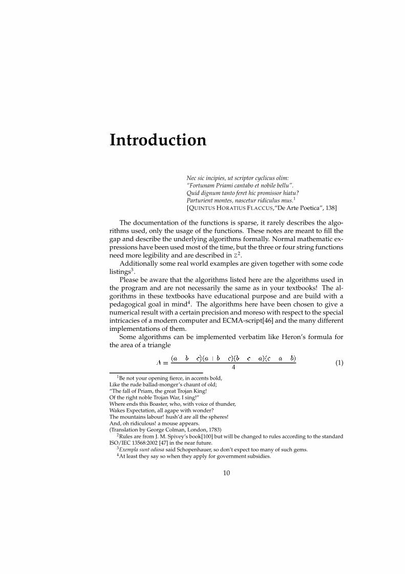
The documentation of the functions is sparse, it rarely describes the algo-rithms used, only the usage of the functions. These notes are meant to fill thegap and describe the underlying algorithms formally. Normal mathematic ex-pressions have been used most of the time, but the three or four string functionsneed more legibility and are described in Z2.
Additionally some real world examples are given together with some codelistings3.
Please be aware that the algorithms listed here are the algorithms used inthe program and are not necessarily the same as in your textbooks! The al-gorithms in these textbooks have educational purpose and are build with apedagogical goal in mind4. The algorithms here have been chosen to give anumerical result with a certain precision and moreso with respect to the specialintricacies of a modern computer and ECMA-script[46] and the many differentimplementations of them.
Some algorithms can be implemented verbatim like Heron’s formula forthe area of a trianglep I �q9srt;@rvu�����96rn;xwyu��<�z;{rvuSwy9|�<��u}rn9~wv;<�� (1)
1Be not your opening fierce, in accents bold,Like the rude ballad-monger’s chaunt of old;“The fall of Priam, the great Trojan King!Of the right noble Trojan War, I sing!”Where ends this Boaster, who, with voice of thunder,Wakes Expectation, all agape with wonder?The mountains labour! hush’d are all the spheres!And, oh ridiculous! a mouse appears.(Translation by George Colman, London, 1783)
2Rules are from J. M. Spivey’s book[100] but will be changed to rules according to the standardISO/IEC 13568:2002 [47] in the near future.
3Exempla sunt odiosa said Schopenhauer, so don’t expect too many of such gems.4At least they say so when they apply for government subsidies.
10
Introduction Introduction
This is implemented as �1 Math . triangleAreaHeron = function ( a , b , c ) �2 var one = a+b+c ;3 var two = a+b � c ;4 var three = b+c � a ;5 var four = c+a � b ;6 return ( one � two � three � four ) /4;7 � ; �
The formula has been parted for better legibility but it is the verbatim transla-tion of Heron’s formula to ECMA-script.
On the other side there are some occasions where a literal translation is notpossible or not optimal. The former holds for every function of the real lineor above if we assume the the number of possible steps of a Turing machineis at most countable. The latter is the case in the implementation of the partialharmonic function D "C for exampleD "C I C� ��� " ) � (2)
This formula works well for small � up to about )��!�!� but for larger values of� the naıve algorithm loses a lot of precision because of the division of ) bymore and more larger numbers. The individual losses at every division stepaccumulates. Only slowly, but they add up until the point where a simpleasymptotic series not only suffices but is also more precise.
Christoph Zurnieden
PRAGMATIC MATHEMATICAL SERVICE 11

Chapter 1
Special Data Types
1.1 Matrix
The Matrix class handles dense complex matrices numerically. Several oper-ations are implemented. The basic operations are described in chapter 3.1 andthe operations for linear algebra in chapter 5.
1.1.1 Usage of the Class
Instantiation
A new matrix can be installed by generating a new instance of the Matrixclass or via a specially formated string. The Matrix class offers several specialmatrixes and suffers a bit from featuritis bombasti but is nevertheless still useful.The format of the string to build a matrix might be familiar to some. �
1 var s = ” [1 + 2 . 3 i , 3 + 4 i ; 2 + 0 . 1 i , � 9 � � 9 i ] ” ;2 var m = s . parseMatrix ( ) ; �
The lines above produce the following/ T / matrix� )xr /|� ��� ��r � �/ rn� � )���w��,w�w������
The individual elements 9 ��� of the matrix can be reached directly. The onlydifference is that the counting starts at � . To get the element 9 $�$ the followinglines are necessary. �
1 var s = ” [1 + 2 . 3 i , 3 + 4 i ; 2 + 0 . 1 i , � 9 � � 9 i ] ” ;2 var m = s . parseMatrix ( ) ;3 a l e r t (m. a [ 1 ] [ 1 ] ) ; / / g i v e s ” � 9 ��� 9 i ” �
The special matrices offered are (all values are complex numbers, imaginaryparts are omitted if they are � ):
12
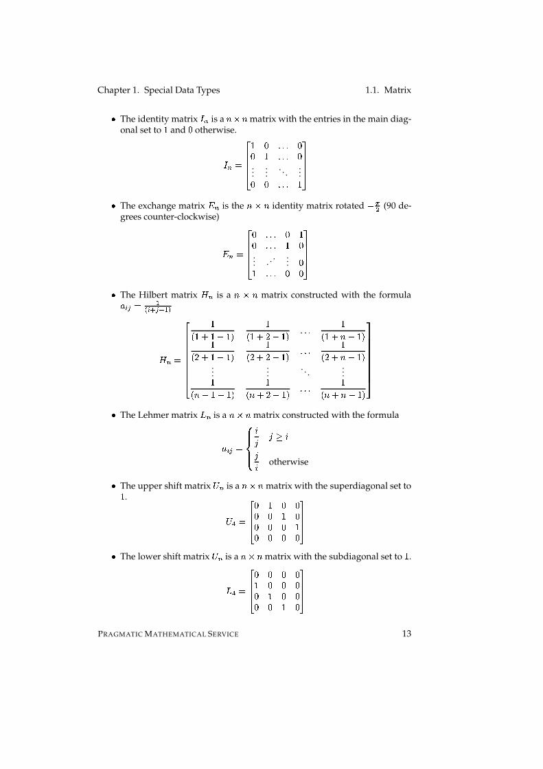
Chapter 1. Special Data Types 1.1. Matrix� The identity matrix � C is a �VT�� matrix with the entries in the main diag-onal set to ) and � otherwise.
�<C�I�� ¡)¢� ����� �� ) ����� �...
.... . .
...�£� ����� )¤¦¥¥¥§
� The exchange matrix ¨�C is the �tT©� identity matrix rotated w#ª $ (90 de-grees counter-clockwise)
¨ C I�� ¡� ����� � )� ����� )¢�... . . .
... �) ����� �£�¤¦¥¥¥§
� The Hilbert matrix D C is a �«T¬� matrix constructed with the formula9 ��� I " �5���<® "°¯D C I � ¡
)�°)±rL)²w�)³� )�°)xr / wt)´� ����� )�4)xr¬�Vw�)³�)� / rL)²w�)³� )� / r / wt)´� ����� )� / r¬�Vw�)³�...
.... . .
...)���µr¶)²w�)³� )���µr / wt)´� ����� )���µr¬�Vw�)³�¤¦¥¥¥¥¥¥¥¥§
� The Lehmer matrix · C is a �eT¸� matrix constructed with the formula
9 ��� I�¹ºº» ºº¼�½ ½�¾ �½ � otherwise� The upper shift matrix ¿ C is a �FTµ� matrix with the superdiagonal set to) . ¿@ÀÁI � ¡ � )Â�£��£� )¢��£�Ã� )�£�Ã�£�
¤ ¥¥§� The lower shift matrix ¿ C is a �GT#� matrix with the subdiagonal set to ) .·}ÀÁI � ¡ �£�Ã�£�)¢�Ã�£�� )Â�£��£� )¢�
¤¦¥¥§PRAGMATIC MATHEMATICAL SERVICE 13
1.2. Complex Chapter 1. Special Data Types� The “empty” matrix Ä is a/ T / matrix with all elements set to Number.NaN
except 9 $�$ which is set to the string "empty"Ä~I �Number.NaN Number.NaNNumber.NaN "empty" �� The zero matrix is a �eT¸� matrix with all elements set to ��rv�!�
1.2 Complex
1.2.1 ÅThe Complex class handles the complex numbers numerically. Because thereal numbers are a proper subset of the complex numbers the complex set isalso called the complex plane.
a = cos
b = sin θ
bθ z
a
ρ
θ
i
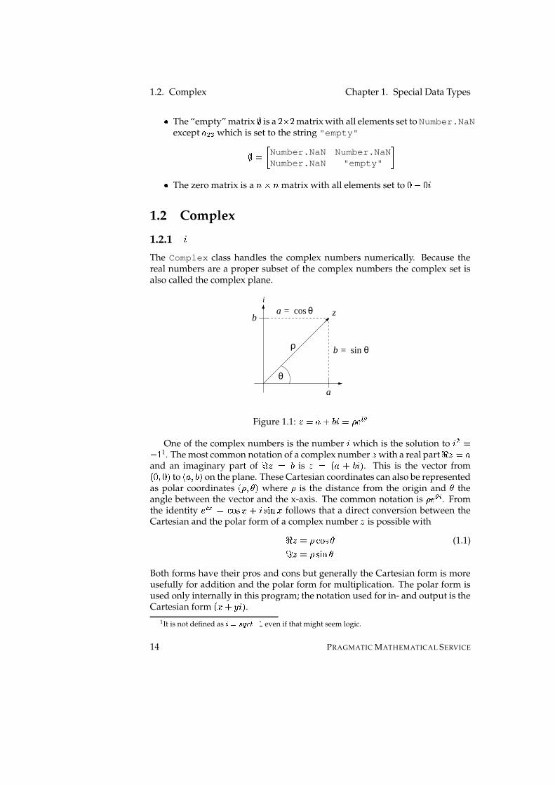
Figure 1.1: ÆÇIL96rt;_�ÈI � 0 �5ÉOne of the complex numbers is the number � which is the solution to � $ Iw6) 1. The most common notation of a complex number Æ with a real part ʱÆËIL9
and an imaginary part of ÌSÆÍIÎ; is ÆÍIÏ�q9OrN;��Ð� . This is the vector from����:��(� to ��9�:_;<� on the plane. These Cartesian coordinates can also be representedas polar coordinates � � :�Ñ(� where � is the distance from the origin and Ñ theangle between the vector and the x-axis. The common notation is � 0 É�� . Fromthe identity 0 ��Ò IÓ%�&('|AVrÔ��'435 ±A follows that a direct conversion between theCartesian and the polar form of a complex number Æ is possible withʱÆÕI � %<&('7Ñ (1.1)ÌSÆÕI � '435 ±ÑBoth forms have their pros and cons but generally the Cartesian form is moreusefully for addition and the polar form for multiplication. The polar form isused only internally in this program; the notation used for in- and output is theCartesian form ��AËr¬Ö��°� .
1It is not defined as ×�ØiÙ�Ú�Û�ÜÞÝ@ß even if that might seem logic.
14 PRAGMATIC MATHEMATICAL SERVICE
Chapter 1. Special Data Types 1.3. Vector
Two conversion functions are implemented to convert the different formsback and forth, namely pol2cart to convert form polar form to Cartesianform and cart2pol for the other direction. Polar to Cartesian (pol2cart)ʱÆÕI � %<&�'�Ñ (1.2)ÌSÆÕI � '�3� ±ÑCartesian to polar (cart2pol)ʱÆÕIRà Æ�à (1.3)ÌSÆÕI«���_�� / �zÌSÆ:�ʱÆ��
Because the real line is a proper subset of the complex plane all complexoperations are mere extensions to the operations on real numbers and thus canbe used as such if the imaginary part is zero. This is usefully for operationsthat are not defined for any real number but for complex ones (for examplewith some inputs to Math.asin()).
1.2.2 Usage of the Class
Instantiation
A new complex number can be installed by generating a new instance of theComplex class. The following lines produce complex numbers, all of the samevalue ��rv�!� : �
1 var i = new Complex ( ) ;2 var j = new Complex ( 0 , 0 ) ;3 var n = 0 ;4 var k = n . toComplex ( ) ;5 var l = n . toComplex ( 0 ) ;6 var s = ”0 + 0 i ” ;7 var m = s . toComplex ( ) ; �
1.3 Vector
The Vector class handles complex vectors numerically.
PRAGMATIC MATHEMATICAL SERVICE 15

Chapter 2
Constants
A short list of more or less useful constants is also included. All constantshave been rounded when more than 37 decimal digits were available. Mostof the mathematical constants have been calculated by the author with 100decimal digits of precision but almost all1 can be found on the net. Some ofthe constants implemented have been omitted if the source is obvious and thedescription in the source-code sufficient. With some exceptions.
2.1 Mathematical Constants
2.1.1 Airy functions
From [1], pp. 446 ff.:
The Airy functions are the solutions to the differential equationá�â â weÆ á IL� (2.1)
Pairs of linearly independent solutions areã 3z�qÆ��<: ã 3z�qÆ�� (2.2)ã 3z�qÆ��<: ã 3z�qÆ(0 $ ª�ä- �ã 3z�qÆ��<: ã 3z�qÆ(0 ® $ ªåä- �1Most probably all, but the author has not looked up all of them, so it has to be “almost all”
16

Chapter 2. Constants 2.1. Mathematical Constants
The ascending seriesã 3Ð�qÆ��{I¶u "<æ �qÆ��Èwyu $�ç ��Æ�� (2.3)ã 3Ð�qÆ��{I . ����u " æ ��Æ��Èweu $ ç �qÆ���� (2.4)æ �qÆ��{Iè)xr )��é Æ�ê}r )²ë �ì é r )²ë � ë�í��é rLë�ë�ë (2.5)IÏî� ? ��ïËð )��ñ ï Æ ê ï�q�(ò7�<éç �qÆ��{I¶ÆÁr /� é Æ À r / ë´óí|é Æ�ô}r / ë´ósë�õ)���é Æ " ��r¶ë�ë�ë (2.6)I î� ? ��ïËð /��ñ ï Æ ê ï � "�q�(ò6r¶)³��éð � r )�*ñ ? Iè)� ïÇð � r )�*ñ ? IN��� � rL)´�<�q� � r � �öë�ë�ë³��� � rv��òÕw / � � arbitrary; ò�IÍ)!: / :��7: �����u " I ã 3Þ���(�{I ã 3Þ�����. �I � ®x÷-=}� $ê � (2.7)
u $ IÍw ã 3 â �q�(�}I ã 3 â ���(�. �I � ® ä-=}� "ê � (2.8)
2.1.2 Apery’s Constant ( ø}ù�úöû )2.1.3 üý�üþ ßÿThe arcus tangent function at "$ .
The value has been calculated via the continuous fraction�����! �ÆÕI Æ)xr Æ $)}r � Æ $��r �(Æ $ó�r ) ì Æ $í²r � $ Æ $���µr¶)³��r¶ë�ë�ë(2.9)
PRAGMATIC MATHEMATICAL SERVICE 17

2.1. Mathematical Constants Chapter 2. Constants
Please see the section about trigonometry in section 3.3
2.1.4 Artins Constant
For the description see E. Artin’s collected papers in [6]. A short oversight is at[117] u�I î�ï�� " � )²w )� ï � � ï wt)´��� � ï is the ò�� prime (2.10)
2.1.5 Backhouse’s Constant
Let ����A�� be a power series whose coefficients � are the primes � C and � ? IÍ) .����A��}I î�ï�� ? � ï A ï ò �OW (2.11)Iè)xr / AËrv�!A $ rtó�A ê rtí�A À r¶)!)�A��}r¶)��!A��}r¶)´í´A ô ë�ë�ëLet ����A�� be ����Aö�}I )����A�� (2.12)I î�ï�� ?�� ï A ï (2.13)IÍ)²w / A�r¬A $ wGA�êxr / A À we�!A � r�í´A � rLë�ë�ë (2.14)
N. Backhouse’s conjecture: � I��53��C�� î����� �C � "� C ���� (2.15)Iè) � � ó ì ��í � � ����� (2.16)
2.1.6 Bernstein’s Constant
If ¨�C*� æ � is the error of the best approximation to a real function æ ��A�� on theinterval ��w6)!:�)�� by real polynomials of degree at most � and � ��Aö�#I à AÈà thenBernstein showed in [11] that� �^/ ì í±ë�ë�ë! "��3#�C$� î ��¨ $ C*� � �% Ô� �^/ õ ì ����� (2.17)
Many people had refined the underlying theory and augmented the numericapproximation of the constant &}� "$ � . The number used here has been calculatedon the principles shown in [20](section 2).
Bernstein himself established the upper and lower bounds 25 years later in[10] as &x� � �% =x� / � ��à '��Þ�{� ��� ��à� for 9)(�� (2.18)
18 PRAGMATIC MATHEMATICAL SERVICE
Chapter 2. Constants 2.1. Mathematical Constants
=}� / � �åà '��Þ�{� ��� ��à� * )²w )/ � w�),+ -&}� � � for 9.( )/ (2.19)
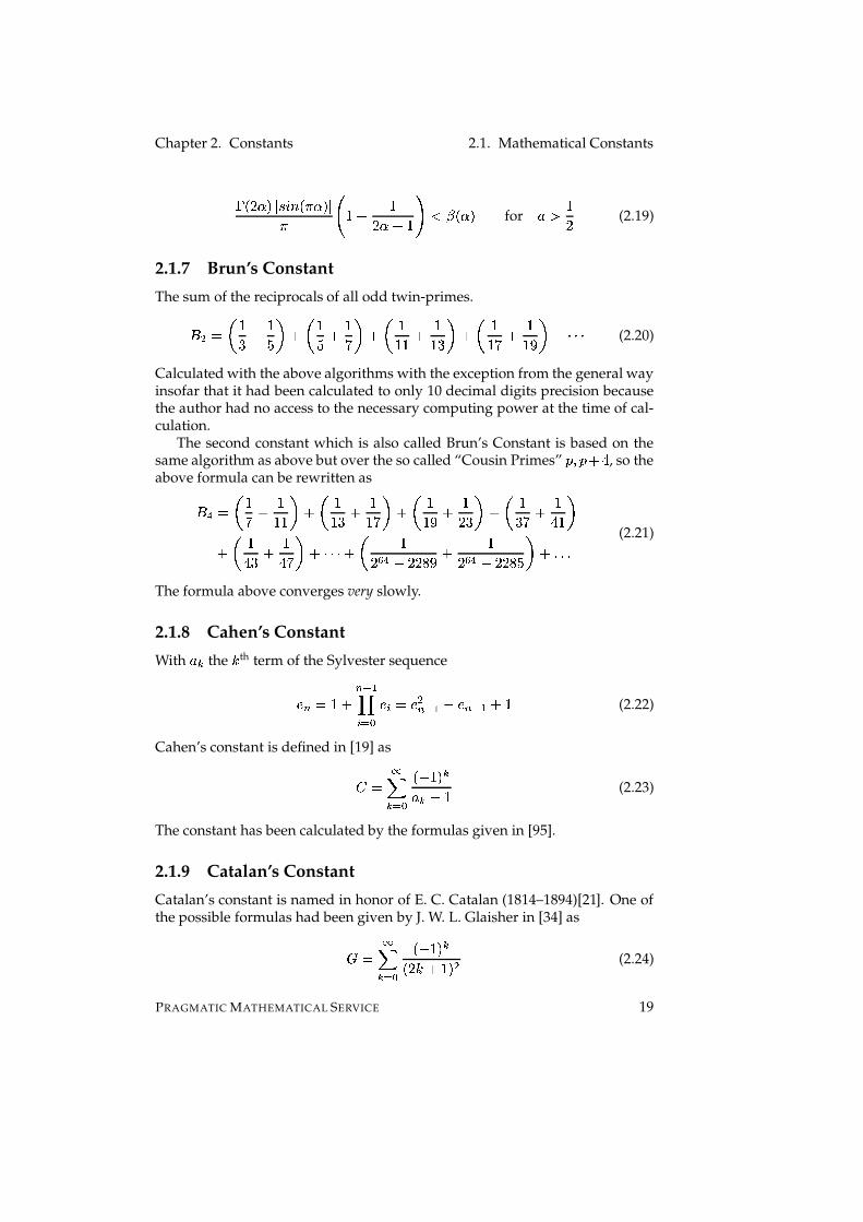
2.1.7 Brun’s Constant
The sum of the reciprocals of all odd twin-primes.� $ I ð )� r )ó ñ rÓð )ó r )í ñ r�ð ))() r ))³� ñ r�ð ))´í r ))�� ñ r¶ë�ë�ë (2.20)
Calculated with the above algorithms with the exception from the general wayinsofar that it had been calculated to only 10 decimal digits precision becausethe author had no access to the necessary computing power at the time of cal-culation.
The second constant which is also called Brun’s Constant is based on thesame algorithm as above but over the so called “Cousin Primes” � : � r � , so theabove formula can be rewritten as� À I ð )í r ))()7ñ r�ð ))�� r ))�í�ñ rÓð ))�� r )/ �*ñ rÓð )��í r )� )7ñr ð )� � r )� íñ r¶ë�ë�ë³r ð )/ � À w /(/ õ(� r )/ � À w /!/ õ�ó�ñ r ����� (2.21)
The formula above converges very slowly.
2.1.8 Cahen’s Constant
With 9 ï the ò th term of the Sylvester sequence0´C�IN)xr C® "�� � ? 0 � I«0 $C ® " wy0´C ® " r¶) (2.22)
Cahen’s constant is defined in [19] as/ I î�ï�� ? �4w6)³� ï9 ï w�) (2.23)
The constant has been calculated by the formulas given in [95].
2.1.9 Catalan’s Constant
Catalan’s constant is named in honor of E. C. Catalan (1814–1894)[21]. One ofthe possible formulas had been given by J. W. L. Glaisher in [34] as0 Ilî�ï�� ? �4w6)³� ï� / ò6r¶)³� $ (2.24)
PRAGMATIC MATHEMATICAL SERVICE 19
2.1. Mathematical Constants Chapter 2. Constants
The formula used to compute the numerical approximation was0 I � õ �5 1 / r . ��2�r î�ï�� ? òöé $� / ò���é � / ò~r¶)³� $ (2.25)
2.1.10 Champernown’s constant
Champernown’s constant/
is build by concatenating the positive natural inte-gers. With 3 the concatenation operator and �4�iW the decimal representationof Champernown’s constant is/ I¶� � )53 î6C � $87 � � ) / � � ó ì í@õ{�±)��±)()@) /S����� (2.26)
The resulting real is transcendental and a simple normal number in base 10. Anormal number is a real number with its digits showing a uniform distributionin all bases and a simple normal number is a number in base ; with its digitsappearing with probability " 9 .2.1.11 Continued Fraction Constant
In a posting to the Math–fun list ([40]) Bill Gosper said:
By strange coincidence, the information in a typical continued frac-tion term is very nearly one decimal digit—actuallyu�I )ì � $�5 å� / �!�5 å�°)³�(� (2.27)
2.1.12 Conway’s Constant
Conway’s Constant describes the rate of growth of the number of digits in thelook–and–say sequence. This sequence is an integer sequence with the term �xr¸)“describing” the term � . Starting with � ? IÍ) :� ? Iè) (2.28)� " Iè)!) ”one” 1 (2.29)� $ I / ) ”two” 1s (2.30)� ê Iè) / )!) ”one” 2, ”one” 1 (2.31)�����
(2.32)
20 PRAGMATIC MATHEMATICAL SERVICE
Chapter 2. Constants 2.1. Mathematical Constants
It is the unique real root of the polynomial�~I¶Aô " weA �;: w / A �;< weA � ôxr / A �;� r / A �;� rvA � À weA � ê²wGA � $ wGA � " wGA � ?weA �;: r / A �;< rtó�A � ô rn��A �;� w / A �=� w�)��!A � À we�!A � ê w / A � $ r ì A � " r ì A � ?rvA À : rv�!A À < wy��A À ô wví´A À � wyõ�A À � wyõ�A À�À rL)³��A À ê r ì A À $ rnõ�A À "w¬ó�A À ? w�) / A�ê : rtí�Aê < w¬í�Aê�ôxrtí�Aê � rvAê � we�!Aê À r¶)���A�ê�ê}rvAê $ w ì A�ê "w / Aê ? w�)���A $ : we�!A $ < r / A $ ôxrv�!A $ � wy��A $ � r¶) � A $ À weõ!A $ ê²w¬í�A $ "rn��A $ ? rn��A " : w � A " < w�)��!A " ô±w¬í�A " � r¶) / A " � r�í´A " À r / A " ê²wt) / A " $w � A "�" w / A " ? rtó�A : r¬A�ô²wví´A � rtí�A � w � A À rL) / Aê±w ì A $ rn��A�w ì(2.33)
The above polynomial is not a mere approximation of the constant but theclosed form. For detailed descriptions see J. H. Conway’s articles in [22] and[23].
2.1.13 Copeland-Erdos’ Constant
Copeland-Erdos’ constant is a variation of Champernown’s constant: not thepositive integers are concatenated but the positive primes.
2.1.14 >�?A@CBThe cosine of ) had been calculated with%�&('7ÆÕI 0 ��D rv0 ®��#D/ (2.34)
2.1.15 >�?A@FEGBThe cosine hyperbolicus of ) had been calculated with%�&('7ÆÕI 0 ��D rv0 ®��#D/ (2.35)I«%<&�'4+����ÐÆ��2.1.16 HI JThe cube root of 2 had been calculated with the ”long hand” method and thehelp of a pencil and several perforated sheets of paper to 101 digits accuracy bythe author while he was suffering from the symptoms of a visit to a restaurantwith surprisingly bad hygienics.
PRAGMATIC MATHEMATICAL SERVICE 21

2.1. Mathematical Constants Chapter 2. Constants
2.1.17 HI úThe cube root of 3 had been calculated with Perl’s implementation of big in-teger and big floating point numbers and Newton’s method. All steps weredone with fractions K L to make use of the absolute precision of integer arith-metic. Only the last step was done by computing the division out to get adecimal representation.
2.1.18 Dubois-Raymond Constant
One of the remarkable numbers to be found in [59] is the second Dubois-Raymond constant / I 0 $ w’/ (2.36)
2.1.19 Euler-Mascheroni Constant MThis constant, also known as Euler’s constant, is defined as the limit of� I��53��C$� î � C�ï�� " )ò wN�� ²� � (2.37)
The identity with the harmonic numbers� IO��3#�C$� î �zD C wN�5 ²�å� (2.38)
makes this constant useful for computing several related functions like the har-monic function itself in section 4.10.4.
2.1.20 Embree-Trefethen Constant
The Embree-Trefethen constant is the generalized form of Viswanath’s constantdescribed in 2.1.71. For the recurrenceA C � " I¶A CQP &�A C ® " with 9 ? I¶��:�9 " Iè)(:=��� sign �}I )/ (2.39)
a limit exists for almost all values of &R �&��}IO��3#�C$� î à AÈà äS (2.40)
The critical value &UT such that R �V&UT��vI�) is sometimes called the Embree-Trefethen constant because of[24].
Viswanath’s constant can be found at R �°)´� .22 PRAGMATIC MATHEMATICAL SERVICE

Chapter 2. Constants 2.1. Mathematical Constants
2.1.21 Erdos-Borwein Constant
The Erdos-Borwein constant, named after Paul Erdos and Peter Borwein is thesum of the reciprocals of the Mersenne numbers.¨XWnI î�C � " )/ C w�) (2.41)
2.1.22 YThe constant 0 , also known as Napier’s constant, is the base of the naturallogarithm.
The most common descriptions are0sI î�C � ? )�@é (2.42)
0sI"�53��Ò � î ð )xr )A ñÒ
(2.43)
The equation 2.42 is due to [?].There is a nice, albeit non-simple continued fraction representation of 00ÁI / r ))xr )/ r /��r �� r �ó�r¶ë�ë�ë
(2.44)
2.1.23 Gompertz’ constant
Gompertz constant 0[Z]\ î? 0 ®A^)xr`_ba _ (2.45)IÍw�0dc{3z�°w6)³� (2.46)c}3q��Aö� is the exponential integral.A simple continued fraction has been foundby Stieltjes[101] 0 I )/ w ) $� w / $ì w � $õ,w�ë�ë�ë
(2.47)
PRAGMATIC MATHEMATICAL SERVICE 23
2.1. Mathematical Constants Chapter 2. Constants
2.1.24 Feigenbaum Constants
Theory
The Feigenbaum constants describe the ratios in a bifurcation diagram. Theconstant e is a universal constant for functions approaching chaos via perioddoubling, discovered by Mitchel Feigenbaum in [26] with the iterationæ ��A��}IN)²w à AÈà f (2.48)
With C the point of the/ C -cycle, î the value of C at g and under the as-
sumption of geometric convergence�53��C$� î î w C�I çe C (2.49)
Solving for e with ç constant and eh( )e6I��53#�C$� î C � " w C C � $ w C � " (2.50)
The Feigenbaum constant � is the separation of adjacent elements from onedoubling to the next � Ii�53#�C$� î j Cj C
� " (2.51)
with j C the value of the element closest to zero in the/ C -cycle 2.
The constants given in the implementation for e and � are for the logisticmap æ ��A��}Iè)²w à AÈà $ (2.52)
The other constants, ;´:�u�: j , were given by [17] in an email to Simon Plouffe3.With æ ��A�� and ç ��A�� even functions æ ���(�{I ç �q�(�{IN) , e as large as possible andç � � A��� I ç � ç ��A���� (2.53)e æ � � A��� I ç â � ç �qA���� æ ��Aö�år æ � ç ��Aö��� (2.54)
together with ç �z;<�{I«�6I )ç ��u{r j �°� with k´;�:�u�: j,l �i[�
(2.55)
while k�;´:�u $ r�; $ l are minimal. With m the order of the nearest singularity andz approaching zero )ç �qu@r j �örnÆ�� Ion���Æ!p(� (2.56)
2vid. [16, 86] for both constants3With Keith Briggs, David Bailey and Steven Finch listed as the recipients of a quite pale carbon
copy
24 PRAGMATIC MATHEMATICAL SERVICE
Chapter 2. Constants 2.1. Mathematical Constantsq q q q q q q qr r r r r r r rFunny Pictures Plotting Bifurcation Diagrams for Highly Pedagogical Aims
To get a Bifurcation diagram4 of the recurrence formula given in [37]A�C � " I � A�C*�°)²weAC�� (2.57)
by on-board means5 two small program-listings might be helpful.At first a standard[45] C program. �
1 # include � s t d l i b . h�2 # include � s t d i o . h�3
4 i n t main ( i n t argc , char �(� argv ) �5 double x = 0 . 0 ;6 double r = 0 . 0 ;7 / / s t a r t must be be tween 0( z e r o ) and 1( one )8 double s t a r t = 0 . 5 ;9 i n t i =0;
10
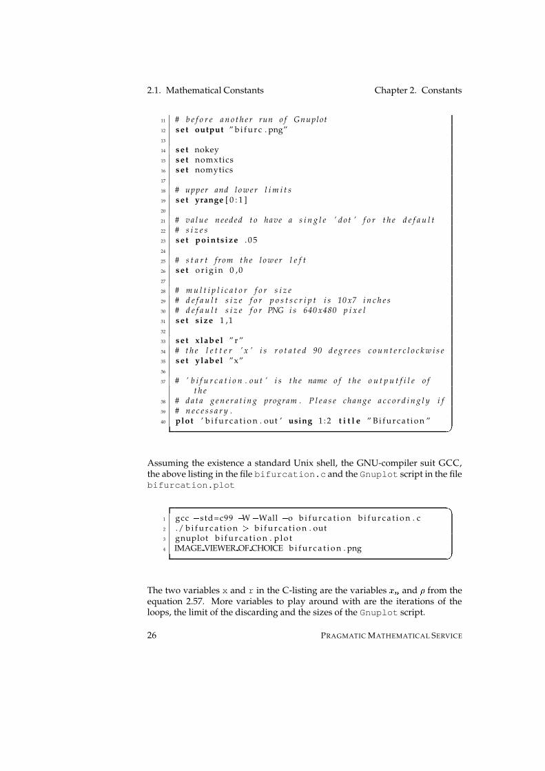
11 for ( r = 0 ; r � 4 ; r += 0 . 0 0 1 ) �12 x = s t a r t ;13 for ( ; i � 500; i ++) �14 x = r � x � (1 � x ) ;15 / �16 Discard t h e f i r s t 450 p o i n t s b e c a u s e t h e17 i t e r a t i o n s need some t ime t o s e t t l e on a18 f i x e d p o i n t .19 � /20 i f ( i � 450) �21 p r i n t f ( ”%f s t%f s n” , r , x ) ;22 �23 �24 �25 e x i t ( EXIT SUCCESS ) ;26 � �
then the listing for Gnuplot �1 # P o s t s c r i p t f i l e s w i l l g e t v e r y l a r g e !2 # s e t term p o s t s c r i p t enhanced ” H e l v e t i c a ” 123 # s e t output ” b i f u r c . ps ”4
5 # D e f a u l t i s PNG with b l a c k t i c k s and r e d d a t a6 # p o i n t s7 s e t terminal png8
9 # Gnuplot w i l l no t o v e r w r i t e ( a t l e a s t with v e r s i o n10 # 3 . 7 p2 ) so t h e f i l e l i s t e d h e r e has t o be d e l e t e d
4A logistic map, to be a bit more exact5At least on-board means of most Unix distributions.
PRAGMATIC MATHEMATICAL SERVICE 25
2.1. Mathematical Constants Chapter 2. Constants
11 # b e f o r e a n o t h e r run o f Gnuplot12 s e t output ” b i f u r c . png”13
14 s e t nokey15 s e t nomxtics16 s e t nomytics17
18 # upper and l o w e r l i m i t s19 s e t yrange [ 0 : 1 ]20
21 # v a l u e needed t o have a s i n g l e ’ d o t ’ f o r t h e d e f a u l t22 # s i z e s23 s e t points ize . 0 524
25 # s t a r t f rom t h e l o w e r l e f t26 s e t o r i g i n 0 ,027
28 # m u l t i p l i c a t o r f o r s i z e29 # d e f a u l t s i z e f o r p o s t s c r i p t i s 10 x7 i n c h e s30 # d e f a u l t s i z e f o r PNG i s 640 x480 p i x e l31 s e t s ize 1 ,132
33 s e t x label ” r ”34 # t h e l e t t e r ’ x ’ i s r o t a t e d 90 d e g r e e s c o u n t e r c l o c k w i s e35 s e t ylabel ”x”36
37 # ’ b i f u r c a t i o n . out ’ i s t h e name o f t h e o u t p u t f i l e o ft h e
38 # d a t a g e n e r a t i n g program . P l e a s e change a c c o r d i n g l y i f39 # n e c e s s a r y .40 plot ’ b i f u r c a t i o n . out ’ using 1 : 2 t i t l e ” B i f u r c a t i o n ” �
Assuming the existence a standard Unix shell, the GNU-compiler suit GCC,the above listing in the file bifurcation.c and the Gnuplot script in the filebifurcation.plot �
1 gcc � std=c99 � W � Wall � o b i f u r c a t i o n b i f u r c a t i o n . c2 ./ b i f u r c a t i o n � b i f u r c a t i o n . out3 gnuplot b i f u r c a t i o n . p l o t4 IMAGE VIEWER OF CHOICE b i f u r c a t i o n . png �
The two variables x and r in the C-listing are the variables A C and � from theequation 2.57. More variables to play around with are the iterations of theloops, the limit of the discarding and the sizes of the Gnuplot script.
26 PRAGMATIC MATHEMATICAL SERVICE

Chapter 2. Constants 2.1. Mathematical Constants
2.1.25 Fibonacci Factorial Constant
The Fibonacci factorial constant t is the infinite producttèI î�ï�� "vu )²we9 ïxw (2.58)
with 9�IÍw )y $ (2.59)
andy
the Golden Ration y I )xr . ó/ (2.60)
2.1.26 Fransen-Robinson Constant
The Fransen-Robinson constant t is defined (vid. [29, 31, 30]) by the integraltÍI \ î? a A=x��Aö� (2.61)
2.1.27 Froda’s Constant
Froda’s constant is simply/�z
. The interesting thing is that he tried to prove itsirrationality in [32]. It is unknown to the author if the prove holds.
2.1.28 Gibbs Constant {,Å�ù}|�ûThe Gibbs- or Wilbraham-Gibbs constant
0 â is the sine-integral with the upperlimit � 0 â I \ î? '�3� %*Ñ a Ñ (2.62)I]~�3Þ� � � (2.63)
There are several functions gathered under the hood of the name “sine-integral”.The variation used here is ~|3z�qÆ��{I \ D? '435 C�� a � (2.64)
From equations 2.62 and 2.64 it is evident that the function '�35 �%*A 6 could bedefined with '435 �%!��A��}I ¹º» º¼
) for A¸I«�'435 ²AA otherwise(2.65)
6sine cardinal with its full name
PRAGMATIC MATHEMATICAL SERVICE 27

2.1. Mathematical Constants Chapter 2. Constants
2.1.29 Gauss-Kuzmin-Wirsing Constant
With t C ��A�� the Gauss-Kuzmin distribution and �Ë���(�{I��Ë�°)´�@I¶��53��C$� î t C ��A��@wN�5 å�°)xrvA��w � I��Ë��Aö� (2.66)
Here � is the Gauss-Kuzmin-Wirsing constant ([124]).Biggs ([12]) computed the constant with the help of the matrix� � ï I �°w²�°� �½ é5�4w / � ï ï� � � ? ð ò �³ñ �°w / � � ���ör / � �� ������r ½ r¶)³� u / �5����� $ w�) w w / ������� $�� (2.67)
with � � ½ , ò��L� , ��A�� C the raising factorial (Pochhammer symbol) and �7��A�� isRiemann’s � -function. [119] gives an example:� $�$ I � � � $ weõ�� í������(�ÈwN"À � $ w ì) ì w�)³ó!������� í��7�q�(�2wN"$ � $ r � �´� (2.68)
The constant is the negative of the absolute value of the second largest Eigen-value of that matrix.
2.1.30 Glaisher-Kinkelin Constant
The Glaisher-Kinkelin constant can be defined memorizable by means of Rie-mann’s � -function([114, 54]) p IL0 ää ÷ ®���� ® "4¯ (2.69)
It can ([35, 36]) also be defined by means of the � -function4.7.9p I��53��C�� î �n����r¶)³�� S ÷÷ � S ÷ � ää ÷ 0��$� ÷� (2.70)
And by means of the0
-function4.7.100 ää ÷p IO��3#�C$� î 0 ���å�� S ÷÷ ® ää ÷ � / � � S ÷ 0 ® ê S ÷� (2.71)
2.1.31 Golden Ratio
The Golden Ratioy y I )xr . ó/ (2.72)
The triangle described by the edges A,B and C in figure 2.1.31 is also called aGolden Gnomon. The ratio of the lengths of the lines 9vI � /
and ;¸I p �is
equal to the Golden Ratio y I 9 ; (2.73)
28 PRAGMATIC MATHEMATICAL SERVICE

Chapter 2. Constants 2.1. Mathematical Constants
α
C
A Bh
Figure 2.1: Pentagon withGolden Gnomon
����������������������������������������������������������������������������������������������������������������������������������������������������������������������������������������������������������������������������������������������������������������������������������������������������������������������������������������������������������������������������������������������������������������������������������������������������������������������������������������������������������������������������������������������������������������������������������������������������������������������������������������������������������������������������������������������������������������������������������������������������������������������������������������������������������������������������������������������������������������������������������������������������������������������������������������������������������������������������������������������������������������������������������������������������
Figure 2.2: Pentagram withGolden Gnomon
Thus the angle � is in radians � I / '�35 ® " ð ;/ 9Èñ (2.74)I )ó � (2.75)
or 36 degrees.Mirroring the triangle at
p �and copying and rotating 36 degrees results in
the pentagram in figure 2.1.31Rotating the triangle at the point ' 36 degrees a sufficient number of times
gives a decagon with a side length of
p �The infinite series for the Golden Ratio is according to [?]y I )��õ r î�C � ? �°w6)´� C
� " � / �#r¶)³�<é����r / �<é �@é � $ C � ê (2.76)
The continued fraction is very simple to memorizey Iè)}r ))xr ))xr ))xr ))xr ))xr¶ë�ë�ë(2.77)
The Golden Ratio has relations with many other functions, for example withthe Fibonacci numbers (with t C the � th Fibonacci number)y Iè)xr î�C � ? �°w6)´� C
� "t�C,tÈC � " (2.78)
PRAGMATIC MATHEMATICAL SERVICE 29

2.1. Mathematical Constants Chapter 2. Constants
which follows from the continued fraction in equation 2.77ACµIÍ)xr )A C ® " (2.79)
with A " IN) and has the obvious solutionACµI t C � "t C (2.80)
so y I��53��C$� î t Ct C ® " (2.81)
Equation 2.81 has been used to calculate the Golden Ratio because it is possibleto calculate it with rationals up to the last point where one Big Float divisionis necessary.
2.1.32 Golomb’s Constant
The Golomb constant [38], also known as the Golomb-Dickman constant, is thelimit of the ratio � IO��3#�C$� î I 9�C� (2.82)
where 9 C is the expected length of the longest cycle in a uniformly distributedrandom permutation of a set � with ���©IL� .
An approximation for 9 C 7 as shown in [82]9�C�I y $ ®�� � �(® " r-� ð � �(® "�5 ²�tñ (2.83)
wherey
denotes the Golden Ration " ��� �$ .
2.1.33 Grothendieck’s Majorant
Grothendieck’s majorant [41] ç I �/ �5 å�4)xr . / � (2.84)
2.1.34 Hadamard-de la Valle-Poussin Constant
More prominently known as the Meissel-Mertens ([71]) or prime reciprocalconstant it is defined by the infinite sum� " I � r î�ï�� " ð �5 u )²w � ® "ï w r )� ï ñ (2.85)
7The sequence is known as the Golomb sequence or Silverman’s sequence
30 PRAGMATIC MATHEMATICAL SERVICE

Chapter 2. Constants 2.1. Mathematical Constants
where � is the Euler-Mascheroni constant and � ï is the ò th prime, or by thelimit � " I"��3#�Ò � î �� �K�� Ò )� wN�� C�5 ²A��� (2.86)
A fast converging series is according to [55]� " I � r î�C � $ ���å�� �5 ~�q�����å��� (2.87)
where �7���å� is Rieman’s � -function and ��Aö� is the Mobius function.
2.1.35 Hafner-Sarnak-McCurley Constant
The Hafner-Sarnak-McCurley constant is the average probability �����å� that thedeterminants of two �yTO� integer matrices are relatively prime.�����å�xIlî�ï�� " ��� )²w �� )²w C�� � " u )²w � ®7�C w �� $ � �� (2.88)� ï is the ò th prime.
With ���°)³� as the average probability that two random integers are relativelyprime ���°)³�{I ì� $ (2.89)
As this is obviously the inverse of �7� / ��I ª ÷� another, exponentially8 converg-ing equation has been found by [28]R Z �53��C�� î �����å�{I î�ï�� $ �7�zò7� ®�¡�¢ (2.90)
2.1.36 Hard-Hexagon Entropy Constant
The hard square hexagon constant mA£ is given bym £ I���3#�C$� î � 0 ���å�4� äS ÷ (2.91)
8at ¤b¥�¦ §�¨�©PRAGMATIC MATHEMATICAL SERVICE 31

2.1. Mathematical Constants Chapter 2. Constantsm £ is algebraic ([8, 49])m�£ÕIom " m $ m ê m À (2.92)m " I � ® " � � ª )() � ªä ÷ u ® $ (2.93)m $ I ð*)²w . )²wyu{r¬« / rvu}r /, )xrvu}rnu $ ñ $ (2.94)m ê I ð*w6)±w . )²wyu{r « / rvu{r / )xrvu{rnu $ ñ $ (2.95)m À I ð . )²we9,r « / rv96r /, )xrn96rv9 $ ñ ® ä÷ (2.96)
9ËI w6) / �� ì � )() ä- (2.97)
;²I / ó���))!)���í�� �!� ä÷ (2.98)
u�I ð )�¸r �õ 9�1��z;2r¶)³� ä- wL�q;xwt)´� ä- 2 ñ ä- (2.99)
This can be summarized to be the unique positive root ofm�£ÕI / ó��(��í � / � ì �7)³Æ $ À r / �7)³� / �(� ì ó|) /(/!/ í´õ � Æ $�$r / ó���ó�� ì / ��)!)´í / � ì í��(í�� / Æ $ ? r�í���í!í / ì!ì �!õ(õ ì!ì(ì ó�õ(�(í���í!í ì Æ " <rtí �!� � � õ(õ!��)��7)³�7)³��õ!�|)³���7) ì �!Æ " � r / ��ó�õ(�7)³ó!�!�(õ!��í ì �(ó�õ / �(�!ó / õ(Æ " Àw¬í / � �(ó ì í�� / õ(ó ì � �|) ì ) ì )´í � �!õ!Æ " $ rL)³��í�)´ó!ó �!� õ�)³ó!� �!� �!��õ(õ�� � � / ì � Æ " ?w¬í|) /(/ �!õ(�!� �!� ) � �(� � �!ó!õ�õ � � / õ!Æ < wví��!� � í � �7)()�õ(� ì �(�|)��!�!õ(í|) � õ�õ(Æ �rv��í�) � �7)³�(ó / í!í���í(í�ó(í�ó7)��!��ó / õ!Æ À wy� / í!ó|) ì �7)³õ7)³� � í����7)³ó���õ�ó�)³ó /(2.100)
The0 ���å� in equation 2.91 is the number of arrays with no adjacent 1s in a
binary �GTO� -matrix� � I � ¡
)Â� ) ������ )¢� �����)Â� ) �����...
......
. . .
¤¦¥¥¥§ (2.101)
The adjacent elements are the set of some 9 ��� Iè)k³9 �V® � l TGk³9�5���V® � :�9 �V® ��� " :�9 �5� " ® ��� " l (2.102)
32 PRAGMATIC MATHEMATICAL SERVICE

Chapter 2. Constants 2.1. Mathematical Constants
The number0 ���å� is also the number of configurations of non-attacking kings
on a �vT©� hexagonal chessboard. A detail of such a board with two possiblecombinations is shown in figure 2.3, the possibles moves of a king accordingsome of the most common rules is shown in figure 2.4.
¯°¯°¯°¯¯°¯°¯°¯¯°¯°¯°¯±°±°±°±±°±°±°±±°±°±°±²°²°²°²²°²°²°²²°²°²°²²°²°²°²²°²°²°²³°³°³°³³°³°³°³³°³°³°³³°³°³°³³°³°³°³
´°´°´°´´°´°´°´´°´°´°´µ°µ°µ°µµ°µ°µ°µµ°µ°µ°µ¶°¶°¶°¶¶°¶°¶°¶¶°¶°¶°¶¶°¶°¶°¶¶°¶°¶°¶·°·°·°··°·°·°··°·°·°··°·°·°··°·°·°· ¸°¸°¸°¸¸°¸°¸°¸¸°¸°¸°¸¹°¹°¹°¹¹°¹°¹°¹¹°¹°¹°¹º°º°º°ºº°º°º°ºº°º°º°ºº°º°º°ºº°º°º°º»°»°»°»»°»°»°»»°»°»°»»°»°»°»»°»°»°»
¼°¼°¼°¼¼°¼°¼°¼¼°¼°¼°¼¼°¼°¼°¼½°½°½°½½°½°½°½½°½°½°½½°½°½°½¾°¾°¾°¾¾°¾°¾°¾¾°¾°¾°¾¾°¾°¾°¾¾°¾°¾°¾¿°¿°¿°¿¿°¿°¿°¿¿°¿°¿°¿¿°¿°¿°¿¿°¿°¿°¿
À°À°À°À°ÀÀ°À°À°À°ÀÀ°À°À°À°ÀÁ°Á°Á°ÁÁ°Á°Á°ÁÁ°Á°Á°Á°°°°Â°°°°Â°°°°Â°°°°Â°°°°ÂðððÃðððÃðððÃðððÃðððÃ
Ä°Ä°Ä°Ä°ÄÄ°Ä°Ä°Ä°ÄÄ°Ä°Ä°Ä°ÄÅ°Å°Å°ÅÅ°Å°Å°ÅÅ°Å°Å°ÅÆ°Æ°Æ°Æ°ÆÆ°Æ°Æ°Æ°ÆÆ°Æ°Æ°Æ°ÆÆ°Æ°Æ°Æ°ÆÆ°Æ°Æ°Æ°ÆÇ°Ç°Ç°ÇÇ°Ç°Ç°ÇÇ°Ç°Ç°ÇÇ°Ç°Ç°ÇÇ°Ç°Ç°ÇÈ°È°È°È°ÈÈ°È°È°È°ÈÈ°È°È°È°ÈÉ°É°É°É°ÉÉ°É°É°É°ÉÉ°É°É°É°ÉÊ°Ê°Ê°Ê°ÊÊ°Ê°Ê°Ê°ÊË°Ë°Ë°Ë°ËË°Ë°Ë°Ë°Ë
Ì°Ì°Ì°Ì°ÌÌ°Ì°Ì°Ì°ÌÌ°Ì°Ì°Ì°ÌÍ°Í°Í°Í°ÍÍ°Í°Í°Í°ÍÍ°Í°Í°Í°ÍΰΰΰΰÎΰΰΰΰÎÏ°Ï°Ï°Ï°ÏÏ°Ï°Ï°Ï°ÏаааÐаааÐаааÐÑ°Ñ°Ñ°ÑÑ°Ñ°Ñ°ÑÑ°Ñ°Ñ°ÑÒ°Ò°Ò°ÒÒ°Ò°Ò°ÒÓ°Ó°Ó°ÓÓ°Ó°Ó°Ó
Ô°Ô°Ô°Ô°ÔÔ°Ô°Ô°Ô°ÔÔ°Ô°Ô°Ô°ÔÕ°Õ°Õ°Õ°ÕÕ°Õ°Õ°Õ°ÕÕ°Õ°Õ°Õ°ÕÖ°Ö°Ö°Ö°ÖÖ°Ö°Ö°Ö°Ö×°×°×°×°××°×°×°×°×
ذذذØذذذØذذذØٰٰٰÙٰٰٰÙٰٰٰÙÚ°Ú°Ú°ÚÚ°Ú°Ú°ÚÛ°Û°Û°ÛÛ°Û°Û°Û
Ü°Ü°Ü°ÜÜ°Ü°Ü°ÜÜ°Ü°Ü°ÜÝ°Ý°Ý°ÝÝ°Ý°Ý°ÝÝ°Ý°Ý°ÝÞ°Þ°Þ°ÞÞ°Þ°Þ°Þß°ß°ß°ßß°ß°ß°ß
Figure 2.3: Hexagonal Chessboard
2.1.37 Khintchine Constant
The Khintchine constant ([52]) is the limit of the geometric mean0 C*�q�ÐA of the
partial quotients 9�C of a continued fraction for �áàâg0 C ��Aö�xIN��9 " 9 $ 9 ê ë�ë�ë�9 C � äS (2.103)
The exact value is difficult to compute, see for example [7] for examples. Oneis � I¬ã�äæå * )�5 / î�C � $ D â$ C
® " � �7� / �å�Èwt) �� + (2.104)
Here, �7�qÆ�� is Riemann’s � -function and D âC is an alternating harmonic number.Not all numbers are equal of course, so some real A exist for which �53�� C�� îèç S Ò ¯;é�ëê ,
for example 0 , . / , . � .
PRAGMATIC MATHEMATICAL SERVICE 33

2.1. Mathematical Constants Chapter 2. Constants
ì�ì�ì�ì�ìì�ì�ì�ì�ìì�ì�ì�ì�ìí�í�í�íí�í�í�íí�í�í�íî�î�î�î�îî�î�î�î�îï�ï�ï�ïï�ï�ï�ïð�ð�ð�ð�ðð�ð�ð�ð�ðð�ð�ð�ð�ðð�ð�ð�ð�ðð�ð�ð�ð�ðñ�ñ�ñ�ññ�ñ�ñ�ññ�ñ�ñ�ññ�ñ�ñ�ññ�ñ�ñ�ñò�ò�ò�ò�òò�ò�ò�ò�òò�ò�ò�ò�òò�ò�ò�ò�òò�ò�ò�ò�òó�ó�ó�óó�ó�ó�óó�ó�ó�óó�ó�ó�óó�ó�ó�óô�ô�ô�ô�ôô�ô�ô�ô�ôô�ô�ô�ô�ôõ�õ�õ�õõ�õ�õ�õõ�õ�õ�õö�ö�ö�ö�öö�ö�ö�ö�ö÷�÷�÷�÷÷�÷�÷�÷ø�ø�ø�øø�ø�ø�øø�ø�ø�øù�ù�ù�ùù�ù�ù�ùù�ù�ù�ùú�ú�ú�úú�ú�ú�úú�ú�ú�úû�û�û�ûû�û�û�ûû�û�û�û ü�ü�ü�ü�üü�ü�ü�ü�üü�ü�ü�ü�üý�ý�ý�ýý�ý�ý�ýý�ý�ý�ýþ�þ�þ�þ�þþ�þ�þ�þ�þÿ�ÿ�ÿ�ÿÿ�ÿ�ÿ�ÿ
�������������������������������������������������������������������������������� ������������������������������������������������������������������������������������������������ ����������������������������������������������������� � � � � � � � � � � � � ��������������������������������������������������������������� ���������������������������������������������������������������������������������������������������������������������������������������������������������������������������������������������������������������������������������������������������������������������������������������������������������������������������� � � � � � �
Figure 2.4: Moves of a king on a hexagonal Chessboard
2.1.38 Khintchine’s Harmonic Mean
Khintchine’s Harmonic mean is a variation of Khintchine’s constant describedin 2.1.37. It is described by the integral� ® " Ii��3#�C$� î �9 ® "" rv9 ® "$ rv9 ® "$ rLë�ë�ë³rn9 ® "C (2.105)
2.1.39 Komornik-Loreti Constant
The Komornik-Loreti constant is the value of � described by)ÁI î�C � " � ï� ï (2.106)
34 PRAGMATIC MATHEMATICAL SERVICE

Chapter 2. Constants 2.1. Mathematical Constants
with � ï the Thue-Morse sequence. This constant is the smallest number in �¦)(: / �for which a unique � -development of the form)�I î�C � " � � ®�� (2.107)
exists ([56]).The constant is also the unique positive real root ofî�ï�� ? ð*)²w )� $ ¢ ñ I ð*)²w )� ñ
® " w / (2.108)
The constant is transcendental ([2]).
2.1.40 Second Order Landau-Ramanujan Constant
If 1²��A�� is the number of positive integers �tA which can be expressed as a sumof two squares, then the following limit exists [58].�"!VI$#��&%OC$� î . �5 ²AA 1���A�� (2.109)
The sums of squares of the first ten positive integers that are expressible as thesum of two squares )�I«� $ r¶) $ (2.110)/ IN) $ r¶) $ (2.111)� I«� $ r / $ (2.112)ó,IN) $ r / $ (2.113)õ6I / $ r / $ (2.114)�6I«� $ rn� $ (2.115))³�6IN) $ rn� $ (2.116))³�6I / $ rn� $ (2.117)) ì I«� $ r � $ (2.118))³õ6I«� $ rn� $ (2.119)
So 1²�4)³��I ) , 1�� / ��I /, 1²� � �ËIU� , 1²�qó(�ËI �
, 1²��õ��ËIUó , 1²�����ËI ì, 1²�°)³�(��I í ,1²�4)����2I«õ , 1²�°) ì �@I¶� , 1²�°)³õ(�@IN)�� . . .
Ramanujan exchanged the lower bound for the series � with a variable
p.
The according equation 1²��Aö�{I¬� !(' \ Ò) a �. �� C� rvÑ���Aö� (2.120)
PRAGMATIC MATHEMATICAL SERVICE 35

2.1. Mathematical Constants Chapter 2. Constants
The constant � !(' is the first order Landau-Ramanujan constant.[?] A fast con-verging formula had been given in [28]� !(' I )' � * � / î�C � " � ð )²w )/ $ S ñ �7� / C �&}� / C � � ä÷ S,+ ä (2.121)
where ����Aö� is Riemann’s � -function and &}��Aö� is Dirichlet’s & -function.The second order Landau-Ramanujan constant
/is the limit�53#�C$� î ��� ²Aö� -
÷�"!(' ð1²��Aö�2w � !('. �5 ²A ñ I / (2.122)
2.1.41 Laplace Limit Constant
The Laplace Limit constant is the point at which Laplace’s formula for Kepler’sequation starts to diverge. It is the unique real root ofæ ��Aö�}I Ö5ã�äæå u . )xrvA $ w)xr . )xr¬A $ (2.123)
2.1.42 Lehmer Constant
The Lehmer constant occurs in the Lehmer cotangent expansion ([60])AOIL%�&�� * î�C � ? �°w6)³� C %�&�� ® " u<C + (2.124)
where u C is the recurrenceu C I«u $C � " rvu C r¶) with � ¾ ) (2.125)
2.1.43 Lemniscate Constant
With the arc length of a lemniscate12.6 with 9�Iè) being'ÁI ). / � ð = ð )� ñ�ñ $ (2.126)
the Lemniscate constant is ([1]) ·nI )/ ' (2.127)
Other constants exists under this name:
First Lemniscate Constant With · the lemniscate constant as described in equa-tion 2.127, the second lemniscate constant is ([59])· " I )/ · (2.128)
36 PRAGMATIC MATHEMATICAL SERVICE

Chapter 2. Constants 2.1. Mathematical Constants
Second Lemniscate Constant With� I "ç and
0the Gauss constant?? the
number · $ I )/ � (2.129)
is sometimes called the second lemniscate constant([105].
2.1.44 Lengyel Constant
With · the partition lattice of a set k³9 ? :�9 " : ����� :�9 C l the maximum element ¨ E ¡�Ò Ik�k³9 ? :�9 " : ����� :�9 C l�l and the minimum element ¨ E � C I k$k$k´9 ? l :�k´9 " l : ����� :�k´9 C l�l ,the number - C denoting the number of chains . with .0/Ô·215k´¨ E ¡<Ò :�¨ E � C l �. satisfies the recurrence relation-@C�I C ® "�ï�� " '����@:_ò7�3- ï with - " Iè) (2.130)
The quotient * ���å�xI -{C*� / �5 / � C � " � 4 5 ÷-���@é^� $ (2.131)
is bound between two constants as � approaches infinity ([62]).
2.1.45 Levy constant
In a continued fraction representation of a number A the nth root of the denom-inator � C of the nth convergent asymptotically approaches a constant when �approaches règ . �53��C$� î � "76 C ¯C I«0 � ª ÷ 6�" $98 :$ � (2.132)
With the exception of the set of A of measure zero[63, 61]. Plouffe ([?]) calledthe exponent of ª ÷" $98 :�$ the Khinchin-Levy constant.
2.1.46 Madelung’s Constant
In determine the energy of a single ion in a crystal the constant�
in the equa-tion ¨NIÍw Æ $ 0 $ �� ��<; * ? (2.133)
is called Madelung constant. Different crystals have different geometric ar-rangements, so Madelungs constant depends on the orientation� I � ï � P � ï * ?* ï (2.134)
Madelung constants for cubic lattice sums are defined by ([67]);�C*� / '´�{I î� âï ä ® =>=>= ® ï S � ® î �°w6)´� ï ä � ?>?>? � ï S�qò $" r¶ë�ë�ë³rtò $C �3@ (2.135)
PRAGMATIC MATHEMATICAL SERVICE 37

2.1. Mathematical Constants Chapter 2. Constants
Where the prime indicates that the summation over ����: ����� :��(� is excluded.For a three dimensional table salt crystal (NaCl); ê �°)´�{I î� âï ä ® ï ÷ ® ï - � ® î �4w6)³� ï ä
� ï ÷ � ï - � " ò $" rtò $ rnò $ê (2.136)�Tyagi has found ([108]) a fast converging sum� Ièw )ì w �� /� � w � �� r )/ . / r = u "< w = u ê< w� - ÷ . / w / (2.137)
î� âï ä ® ï ÷ ® ï - � ® î �°w6)³� ï ä � ï ÷ � ï - ò $" rtò $ rnò $ê A 0³A � 1�õ � ò $" r�ò $ rtò $ê 2#w�)CB (2.138)
The constant factor 2.137 of the equation is good for ten decimal digits on itsown, without the following summation.
The other possible packing for a crystal is hexagonal, for example cesiumchloride (CsCl). The formula for the hexagonal lattice sum D $ � / � has a closedform. D @ � / �{I � �5 �� . � (2.139)
The Madelung constant used in the implementation is that of ; ê �°)´� and thecalculation has been done with the equation 2.137.
2.1.47 Magata’s constant
Let � be the data set k��4)!: / ��:³� / :��(�<:�����:�ó(��:�� � :�í���: ����� :³���@: � C7� l with � C denoting thenth prime. With polynomial fit of degree �Owt)u ? r�u " ��A±w¸)³��r�u $ ��A±w¸)³�<��A±w / ��rµu ê ��A±w#)´�<��ASw / ����A±wÇ���´rië�ë�ëÐrµu C ��A±w#)´�öë�ë�ë³��A±wÕ�å�
(2.140)the sum of the coefficients approach a constant when � approaches g ([68]).
2.1.48 Meissel-Mertens constant
See 2.1.34.
2.1.49 Niven’s constant
Let the prime factorization of a number A �iWyQ k´� l be described byA¸I � C ä" � C ÷$ ë�ë�ë � C ¢ï (2.141)
38 PRAGMATIC MATHEMATICAL SERVICE

Chapter 2. Constants 2.1. Mathematical Constants
then the two functions Då��A��}I¬��3� ���� " :4� $ : ����� :4� ï � (2.142)Dv��A��}I¬��� ä*��� " :4� $ : ����� :4� ï � (2.143)with Dn�°)³�{IED��°)³�{IN) (2.144)
have the following properties ([76]):�53��C$� î )� C�Ò � " Då��A��}Iè) (2.145)
�53��C�� î F CÒ � " D���Aö�@we�. A I � u ê $ w������� (2.146)
�53#�C$� î )� C�Ò � " Dv��A��}I / (2.147)
The constant/
in equation 2.147 is the number known as the Niven constantand has the value / Iè)xr * î�ï�� $ � )²w )�7�zò7� � + (2.148)
2.1.50 Reciprocal of the One-Ninth-Constant
See 2.1.51.
2.1.51 One-Ninth-Constant
The One-Ninth-constant is based on a conjecture later proven to be false.In the beginning was a proof by Schonhage ([93]) that�53#�C$� î � � ? ® C �}I )� (2.149)
with � E ® C Chebychev constants. The conjecture wasG I��53��C�� î � � C ® C7� "76 C I )� (2.150)
The naming of constants follows some weird rules, so this constant was namedthe “one-ninth constant” and, by the same logic, its reciprocal is sometimesknown as “Varga’s constant”.
PRAGMATIC MATHEMATICAL SERVICE 39
2.1. Mathematical Constants Chapter 2. Constants
A first hint, thatGIHI ": was given numerically ([107]), a formal disprove
followed only two years later ([39]). An exact value ofG
is given by ([69])G I¬ã�äæå ����� w� � u . )²wyu $ w�n�qu�� ����� (2.151)
with � the complete elliptic integral of the first kind and u a solution to�n�qò��{I / ¨µ�qò7� (2.152)
with ¨ the complete elliptic integral of the second kind.Another name for this constant has been proposed by Varga ([109]): Halphen
constant. Halphen computed the root ([42]) of the equationî�ï�� ? � / ò6rL)´� $ �°w²A�� ï ï � "°¯J6 $ I¶� (2.153)
With A �¬�q�7:�)´� the unique solution is indeedG
([70])
2.1.52 Paris Constant
For the recursion y C I )xr y C ® " for � ¾ / 1 y " IÍ) (2.154)
Paris had proved in [81] thaty C approaches the Golden Ratio
yat a constant
rate. ��3#�C$� î � y w y C �<� / y � C/ I / (2.155)
So ([27]) / I î�C � $ / yy r y C (2.156)
2.1.53 Parking Renyi Constant
This constant answers the question of how much place is wasted by randomlyparking cars in a street. Because this is a theoretical constant the cars have unitlength, the length of the street is a real number and the cars do not overlap norare they allowed to push. So within the closed interval � �7:�A,� with Ao( ) themean number
� ��A�� of cars that can park on that street is described by ([87])� ��Aö�}I ¹» ¼ � for ���nAá ))xr $Ò�® "LK Ò!® "? � ��Ö7� a Ö for A ¾ ) (2.157)
40 PRAGMATIC MATHEMATICAL SERVICE

Chapter 2. Constants 2.1. Mathematical Constants
The mean density %ÂI �53�� Ò � î M Ò ¯Ò , Renyi’s parking constant, can be de-scribed by \ î? ã�äæå©ð*w / \ Ò? )²we0 ®ONÖ ñ a A (2.158)
While the inner integral is � rè=}����:4Aö��r��� ²A with =x��A�:4Ö7� the incomplete = -function or � r c{3z�°w²Aö��r �� ²A with c}3z��A�� the exponential integral, no other formexist for the outer one. Inserting that in equation 2.158 gives% I«0 ® $3P \ î? 0 ® $3Q ? ® Ò ¯A $ (2.159)I«0 ® $3P \ î? 0 ® $SRUT ®öÒ ¯A $ (2.160)
The above holds in one dimension only, but [80] conjectured that for twodimensions �53#�Ò$® N � î � ��Aå:4Ö7�AÖ I$% $ (2.161)
which is not yet proven nor disproven9.
2.1.54 Smallest Pisot-Vijayaraghavan Number
A Pisot number is a positive algebraic integer greater than 1 allof whose conjugate elements have absolute value less than 1. A realquadratic algebraic integer greater than 1 and of degree 2 or 3 is aPisot number if its norm is equal to P ) . [120]
The smallest Pisot number Ñ " , also known as the Plastic constant, is the positiveroot of Aê²weAµw�)ÁI¶� (2.162)
as shown by [92] and proved by [96] The second smallest Pisot number, foundby [96], is the positive root of A À wGA�ê²wt)ÁI¶� (2.163)
He also showed that Ñ " and Ñ $ are isolated and that the positive roots of thefollowing polynomials are also Pisot numbersA C u A $ weAµw�) w rvA $ wt) for ���Nk³W¬Q k³� l$l (2.164)A C w A C � " wt)A $ w�) for ���Nk³W¬Q k³��:�)!: / l�l 1,& a,a � (2.165)
A C w A C ® " wt)A $ w�) for ���Nk³W¬Q k³��:�)!: / l�l 1,& a,a � (2.166)
(2.167)9At least not known to the author at the date given on the front page of this article.
PRAGMATIC MATHEMATICAL SERVICE 41

2.1. Mathematical Constants Chapter 2. Constants
The numbers have been named by [91] because of the closely related worksof [83, 111] about VXW��(%!��A�� Z AµwZY�A([2.1.55 Plastic Constant
See 2.1.54. As a sidenote: with � the plastic constant the circumference of aSnub Icosidodecadodecahedron with 9ËIN) is)/L\ / �«wt)� wt) (2.168)
2.1.56 Porter constant
Porter’s constant ([85])/ I ì �� /� $ � � �5 / r � � w / �� � â � / �2w / � w )/ (2.169)
Example
With ]Õ�X%e:4�å� the number of steps to compute ^�% a �J%G:��å� by means of the Euk-lidian algorithm and ]Õ�X%e:����xIÍ� if % ¾ � then the value of ]Õ�X% � �å� is definedby the reccurence formula]Õ�X%e:4�å�{I`_ )xra]Õ���@:3% �Ë& a �å� for % ¾ �)xra]Õ���@:3%V� for % �� (2.170)
With fixed � and randomly choosen % the average number of steps is ([55])]Õ���å�{I )� �? � Ecb C ]Õ�X%e:4�å� (2.171)
and it has been shown by [78] that]Õ���å�@I ) / �5 /� �¡ �5 ²�¸w � dfe C G � j �j¤§ r / r )� � dfe C y � j ���¸� j
® "36 � �hg � (2.172)
withG � j � the Mangoldt-function,
y � j � the totient-function and/
the Porterconstant.
2.1.57 Sum of the Product of the Inverse of Primes
This constant is probably better described as the sum of the reciprocals of theprimorials10.
10Which rhymes with factorials not with primordials. As said elsewhere in this article: the name-finding in mathematics is not always fully comprehensible.
42 PRAGMATIC MATHEMATICAL SERVICE
Chapter 2. Constants 2.1. Mathematical Constants
A primorial is defined as the product of all primes � ï up to a given prime� C . � C�� I C�ï�� " � ï (2.173)
More generally with a number � instead of the prime � C��� I ª C ¯�ï�� " � ï (2.174)
where � ���å� is the prime counting function which has the numbers of primesup to the limit � .
The limit of the reciprocals of the primorials is��3#�C$� î )� C�ï�� " � C � 7 � � í��(ó / �!��)´í�)�í���)�õ ����� (2.175)
which is implemented here as the sum of the product of the inverse of primes.This limit ([90]) might be of additional interest�53#�C$� î � � C��Ë� "36 K S I«0 (2.176)
where 0 is the base of the natural logarithm.
2.1.58 Rabbit Constant
The rabbit constant has been named aptly: it is a result of the miraculous gift-edness of rabbits to grow up and reproduce. Despite the biological mecha-nism of the reproduction of rabbits the rabbit sequence starts with one rabbit;a young one even, not able to reproduce before growing older. This singlepre-pubescent rabbit of unknown sex shall be denoted � . A rabbit in legalage shall be denoted ) . With the two mappings � à ) for a rabbit grow-ing up and )¬à )�� for multiplicating bunnies. Following the timeline weget � à )oà )³� à )³�7)]à )³�7)!)³�²ë�ë�ë . Written as a binary fraction gives� � )³�7)!)³�7)³�7)!)³�7)()�� ����� $ which is called the Rabbit constant. The implementationgives the decimal representation � � í��(�!õ!�(� �(� ����� .
The Rabbit constant is related to the Fibonacci sequence by the continuedfraction representation of the constant� �7: / ? : /ji ä : /,i ÷ : /ji - : ����� � (2.177)
where t C are Fibonacci numbers ([4, 33, 94]).
PRAGMATIC MATHEMATICAL SERVICE 43

2.1. Mathematical Constants Chapter 2. Constants
2.1.59 Ramanujan-Soldner Constant
The root of the logarithmic integral �53z��A��±I � is also known as the Ramanujan-Soldner constant 11. With the logarithmic integral defined as the Cauchy prin-cipal value ��3Ð��A��}I$kLl \ Ò? a ��5 C� (2.178)Ii�53#�g �,? + � \ " ®�g? a ��� C� \ Ò" �hg a ��5 C� � (2.179)
and the identity follows ([113, 75])kLl \ Ò? a ��5 C� I \ Òm a ��� C� for A ( (2.180)
2.1.60 Reciprocal Fibonacci Constant
The reciprocal Fibonacci constant is exactly what its name implies: the sum ofthe reciprocals of the Fibonacci numbers t2C� i I î�C � " )t C (2.181)
This constant was proved to be irrational by [5].
2.1.61 Reciprocal Prime Constant
See 2.1.34.
2.1.62 Robbins’ Constant
This constant is the average distance of two randomly chosen points inside aunit cube. More exact ([89])n ���(�{I ))���ó A � r¶)´í . / w ì . ��r / )ë�5 .1!)xr . / 2�r � / �5 .1 / r . �x2¸w¬í � B
(2.182)A useful identity is probably�5 1 )xr . / 2 I¶�('435 7+,) (2.183)
It might be of interests to the more claustrophobic readers that the averagedistance of two randomly chosen points on different faces of the cube is [14, 15]n i �q�(�{I )í�ó A )xrL)�í . / w ì . ��r / )ë�� 1 )xr . / 2 r � / �� 1 / r . � 2 wví � B
(2.184)11But o is also found here and there
44 PRAGMATIC MATHEMATICAL SERVICE
Chapter 2. Constants 2.1. Mathematical Constants
The ratio of these two is n i ���(�{I íó n ����� (2.185)
2.1.63 Smallest Known Salem Number
The smallest Salem number is the largest root ofA " ? rvA : weAô�wGA � wGA � weA À weAê±r¬AËr¶) (2.186)
2.1.64 Sierpinski Constant
The Sierpinsky constant � can be described by ([97])� Ii��3#�C$� î � C�ï�� " * $ �qò��ò w � �5 ²� � (2.187)
where * $ ��Aö� is the number of ways to represent the number A asAOI¶9 $ rn; $ for k³9�:�; l �VW (2.188)
2.1.65 @qpqþ�BThe sine of ) had been calculated with'�3� �ÆÕI 0 ��D we0 ®ö��D/ � (2.189)
2.1.66 @qpqþUEáBThe sine hyperbolicus of ) had been calculated with'435 �ÆÕI 0 �#D wy0 ®��#D/ � (2.190)Ièw²��'�3� 7+����ÐÆ��2.1.67 Traveling Salesman Constant
The length of a self-avoiding space-filling curve through a set of � points.� I ��3#�E � î · E. � E (2.191)I � u )xr / . / w . ó7))³ó!� (2.192)
with · E the curve length at the mth iteration and � E the size of the point set([77])
PRAGMATIC MATHEMATICAL SERVICE 45

2.1. Mathematical Constants Chapter 2. Constants
2.1.68 Tribonacci Constant
The Tribonacci sequence is one generalization of the Fibonacci sequence]*C�Ir]*C ® " rs]*C ® $ rs]*C ® ê with ] " It] $ Iè)(:7] ê I / and � ¾ � (2.193)
It has a corresponding constant, the positive root of the polynomial�~ILA�ê²wGA $ weAµwt) (2.194)
Continuing with this technique12
Polynome Constant Name�~ILA $ wGA#wt) "$ u )xr . ó w Fibonacci�~ILA ê wGA $ weAµwt) "ê A )xr - )��,wy� . �!��r - )³�²rn� . �(� B Tribonacci�~ILA À wtë�ë�ë�weAµw�) 7 ) � � / í!ó ì )³��í!ó Tetranacci�~ILA � wtë�ë�ë�weAµw�) 7 ) � � ì ó!� � õ / � ì Pentanacci�~ILA � wtë�ë�ë�weAµw�) 7 ) � �(õ!��ó�õ / õ � � Hexanacci�~ILA ô wtë�ë�ë�weAµw�) 7 ) � �(�7)³� ì � )�� ì Heptanacci�~ILA C weA C ® " w�ë�ë�ë�wGA#wt) 2 � -anacci
2.1.69 The A.G.M of B and ßu ÿThe Gauss constant
0is the reciprocal of the arithmetic-geometric mean of )
and. / 0 I )� u )(: . / w (2.195)
I . /� � ð ). / ñ (2.196)
I )� / � � -÷ � = ð )� ñ � $ (2.197)
where �n��A�� is the complete elliptic integral of the first kind and =}���� the = -function.
A series, converging quite fast is given by [27]0 I / ª� 0 �$�- * î�C � ® î �°w6)³� C 0® $ C ª ê C � "4¯ + $ (2.198)
The constant �. / (2.199)
is called the ubiquitous constant in some articles ([99, 27])12The names of the constants are due to [121]
46 PRAGMATIC MATHEMATICAL SERVICE

Chapter 2. Constants 2.1. Mathematical Constants
2.1.70 Universal Parabolic Constant
F
x
y
v
a
ll1 2
cb−1
0
1
2
3
4
5
6
7
8
−6 −4 −2 0 2 4 6
Figure 2.5: Parabola "À A $ r¶)The universal parabolic constant � is the ratio between the length of the
line # " # $ , the latus rectum and the length of the segment of the parabola # "<v # $ infigure 2.5. The exact value is�èI . / r �� 1!)xr . / 2 (2.200)I . / rn�!'�3� �+s) (2.201)
2.1.71 Viswanath’s Constant
The Viswanath constant is a special form of the Embree-Trefethen constant de-scribed in section 2.1.20.
For the recurrence9 C I P 9 C ® " P 9 C ® $ with 9 ? I¶�7:�9 " Iè)!:;��� sign �{I )/ (2.202)
exists almost surely the limit ([112])�53��C$� î S à 9öà (2.203)
PRAGMATIC MATHEMATICAL SERVICE 47

2.2. Physical Constants Chapter 2. Constants
2.1.72 Weierstrass Constant
The Weierstrass constant á is defined as the value "$ R �4),w�)!:4�°� of Weierstrass’sigma function R �qÆxw � " : � $ � . It has the closed form ([115, 116])á I / ª� . � 0 � y= $ u "À w (2.204)
2.1.73 Some ø Values
Some of the more useful �7���å� values of mostly odd � are implemented. Formore information about Riemann’s � -function and the numerical evaluation ofit see section 4.10.1.
2.2 Physical Constants
This section lacks a lot of bibliographical links, but it is difficult to get the handson the original works. Most of the older books are only available as abridgedtranslations13.
2.2.1 Astronomical Unit
The astronomical unit
p ¿ is the mean distance between Earth and sun. Moreformal: the radius of an unperturbed circular orbit a massless object wouldrevolve about the sun in
$ ªï days. The Gaussian constant ò is defined exactlyas � � �7)�í / � / �(�!õ(�(ó in this case. ([74])
2.2.2 Avogadro Constant
The Avogadro constant z ) is the number of atoms in � � �7) / kg of C " $ and thecurrent value is ([79])ì � � /!/ ) � )´í��~TG)³� $ ê mol
® " P � � ��TG)³� " ô (2.205)
2.2.3 Boltzmann Constant
The Boltzmann constant ò describes the relation between the macroscopic tem-perature and the microscopic particle energy. It is the ratio of the gas constant{
and the Avogadro constant z ) ò�I {z ) (2.206)
13And sometimes bad translations! The author has read a translation of some work of New-ton which could be clearly judged as wrong even without knowning the original text at all—themathematics were glaring wrong.
48 PRAGMATIC MATHEMATICAL SERVICE

Chapter 2. Constants 2.2. Physical Constants
2.2.4 Candela
The definition of a candela14
The candela is the luminous intensity, in a given direction, ofa source that emits monochromatic radiation of frequency ó � �GT)�� " $ Hz and that has a radiant intensity in that direction of "�=< ê wattper steradian.
A wax candela emits about one candela hence the now historic name.
2.2.5 Dielectric Constants
The dielectric constant f is the ratio of the static permitivity of the material @and the electric constant ? f I @ ? (2.207)
The values given in the implementation are the values of @ .2.2.6 Dirac Constant
The Dirac constant | is related to Planck’s constant D by the ratio|ËI D/ � (2.208)
2.2.7 Gas Constant
The gas constant is related to the Boltzmann constant but measures the energyof one mol of particles instead of single particles.
2.2.8 Weight of One Mol Water
The Avogadro constant times the average atomic mass of water–about 18 grams.The word “average” is very important because the composition of water canvary between H "$ O " � and H
$$ O " < or even H ê$ O " � !2.2.9 Speed of Light
The speed of light is fixed at/ �(�xí�� / � ó!õ m
s to have a steady point in spacetimeto hang up the physicist’s hat.
More formal: the meter is defined as15
The metre is the length of the path traveled by light in vacuumduring a time interval of )f} / �(�xí�� / � ó!õ of a second.
1416th CGPM 1979, resolution 31517th CGPM 1983, resolution 1
PRAGMATIC MATHEMATICAL SERVICE 49

2.2. Physical Constants Chapter 2. Constants
So it follows that the speed of light is exactly/ �!�xí�� / � ó�õ m
s . The second is de-fined as16
The second is the duration of ��)�� / ì �7)2í!í�� periods of the radi-ation corresponding to the transition between the two hyperfinelevels of the ground state of the caesium 133 atom.
This definition is not complete, so at the 1997 meeting of the CIPM it was amade clear that:
This definition refers to a caesium atom at rest at a temperatureof 0 K.
2.2.10 Light Year
The year in this implementation is defined to be � ì ó �^/ ó days with/ �
hours ina day,
ì � minutes in an hour andì � seconds in a minute. A lightyear is the
length a photon travels in one year, so the length of a lightyear might differfrom the numbers in other implementations.
2.2.11 Magnetic Permeability of the Vacuum
The magnetic permeability of the vacuum ? follows from the definition of theAmpere and is therefore defined as ? defI � � TG)³� ô N
A$ (2.209)
2.2.12 Newton’s Gravity Constant
Newton’s gravity constant is the proportional constant0
intèI 0 % " % $* $ (2.210)
where t is the force, % " and % @ are masses («� and * is the distance betweenthe masses.
2.2.13 Parsec
Parsec is short for parallax second.�èI ¿ ) ë�%�&���ð / � ) â â� ì �©ñ (2.211)I ¿ ) ë�%�&�� ð / � � � �!�(� / í(í!í�õ� ì � ñ (2.212)
with ¿ ) the astronomical unit.1613th CGPM 1967/68, resolution 1
50 PRAGMATIC MATHEMATICAL SERVICE
Chapter 2. Constants 2.2. Physical Constants
2.2.14 Planck Constant
The Planck constant D is the ratio between the energy of a photon ¨ and itsfrequency � D#I ¨ � (2.213)
2.2.15 Seconds in a Year
Because the term year is ambiguous and variable17 this constant is offered inthis implementation and is the number of seconds in a year of � ì ó �^/ ó days ofõ ì � �(� seconds per day.
2.2.16 Stefan-Boltzmann constant
Also known as Stefan’s constant it is exactlyR I / � � ò À)³ó,D ê u $ (2.214)
with D Planck’s constant, ò Boltzmann constant and u the speed of light. It isthe constant in the Stefan-Boltzmann law of energy flux of a black-body~ I R ] À (2.215)
with ] the absolute temperature of the black-body.
2.2.17 Luminosity of the Sun
Implemented here is the defined value18.
2.2.18 Electric Constant
The electric constant ? is defined as ? defI ) ?³u $ (2.216)
with ? the magnetic constant and u the speed of light.
2.2.19 Wien’s displacement constant
Wien’s displacement constant ; is the ratio between the wavelength of the emis-sion peak of a black-body and the temperature of this black-body;²I � ] (2.217)
With � the emission’s peak wavelength and ] the absolute temperature of theblack-body.
17Sidereal year? Tropical year? Which planet are you even talking about?18The sun is a slightly variable star, so the luminosity varys
PRAGMATIC MATHEMATICAL SERVICE 51
Chapter 3
Common Functions
3.1 Basic operations
The basic functions are defined here as the mathematical functions in the ECMA-standard with the exception of the trigonometric functions which have theirown section. This program extends these functions to the complex plane withthe restriction that ECMA-script in its current version does not allow overload-ing of all functions, so the syntax for the complex arithmetic is different.
3.1.1 Operations on complex numbers
Equality
Two complex numbers Æ " and Æ $ are equal if and only if the real and the imag-inary parts are equal.Æ " I«Æ $ iff 汮 " I 汮 $ 1�ÌSÆ " I«ÌSÆ $ (3.1)
Addition
The addition of complex numbers in their Cartesian notation works like vectoraddition because, well, they are vectors.Æ " rnÆ $ ILÆ ê I _ 汮 ê I¶Ê±Æ " rt汮 $ÌSÆ ê I«ÌSÆ " r�ÌSÆ $ (3.2)�
1 var z 1 = new Complex ( 2 . 3 , � 3.4) ;2 var z 2 = new Complex( � 7.3 , 3 . 8 ) ;3 var z 3 = z 1 . add ( z 2 ) ; �
Subtraction works accordingly ( Æ " .sub( Æ $ )).
52

Chapter 3. Common Functions 3.1. Basic operations
Multiplication
There are mainly two different ways two multiply two complex numbers: theone with the Cartesian notation and the one with the polar form. The polarform is easier to calculate manually but lacks precision when used with Gaus-sian integers1 because of the use of 0 .
The algorithm for the Cartesian form ÆÕI �qʱÆÁr�ÌSÆ��Æ " ë�Æ $ I¶Æ ê I _ 汮 ê I«Ê±Æ " ë�汮 $ wvÌSÆ " ë³ÌSÆ $ÌSÆ ê I ÌSÆ " ë�汮 $ rt汮 " ë³ÌSÆ $ (3.3)
The algorithm for the polar form ÆÕI � 0 É��Æ " ë�Æ $ I¶Æ ê I � D ä � D ÷ u 0 É3� ä ��É7� ÷ w (3.4)
The algorithm used in the program is the Cartesian because of the reasonslisted above.
Division
The rules for division are obviously the same as for multiplication and there aremainly two ways to divide. The algorithm for the Cartesian form ÆÇIè�zʱÆör�ÌSÆ��
Æ "Æ $ I«Æ ê I ¹ºººº» ºººº¼Ê±Æ ê I �q汮 " ë´Ê±Æ $ r�ÌSÆ " ë´ÌSÆ $ ��4�z汮 $ � $ r«�zÌSÆ $ � $ �ÌSÆ ê I �zÌSÆ " ë´Ê±Æ $ rt汮 " ë´ÌSÆ $ ��4�z汮 $ � $ r«�zÌSÆ $ � $ � (3.5)
The algorithm for the polar form ÆÕI � 0 É��Æ "Æ $ I«Æ ê I �D ä� D ÷ u 0 É3� ä ®öÉ7� ÷ w (3.6)
1Gaussian integers are complex numbers with both the real and integer part integer
PRAGMATIC MATHEMATICAL SERVICE 53
3.1. Basic operations Chapter 3. Common Functions
Actually, the algorithm used for division is a third one. It is slightly less precise(about one decimal digit) but avoids overflow
Æ "Æ $ ILÆ ê I¹ººººººººººººººººº» ººººººººººººººººº¼
à ÌSÆ " à ¾ à ÌSÆ $ à ¹ºººº» ºººº¼Ê±Æ ê I )1 汮 $ rÔÌSÆ $x� D ÷� D ÷ 2 ð汮 " r�ÌSÆ " ÌSÆ $汮 $ ñÌSÆ ê I )1 汮 $ rÔÌSÆ $x� D ÷� D ÷ 2 ð�ÌSÆ " w¬Ê±Æ " ÌSÆ $汮 $ ñ
otherwise ¹ºººº» ºººº¼Ê±Æ ê I )1³Ê±Æ $ � D ÷� D ÷ r�ÌSÆ $ 2 ð汮 " 汮 $ÌSÆ $ rtÌSÆ " ñÌSÆ ê I )1 ÌSÆ $ � D ÷� D ÷ r�ÌSÆ $ 2 ð汮 " 汮 $ÌSÆ $ wy汮 " ñ
(3.7)
Power
To get the power of complex numbers is not so easy but solvable, even withcomplex exponents.
In case the exponent is a real number A it is easyÆ Ò I¶0 Ò 8 : D (3.8)
When the exponent is complex too, it is still not that complicated. �jW�^�qÆ�� is�7D�0��°9 from the polar form and thus �,W3^xÆÕI¶������ / �zÌSÆ:�ʱÆ�� .Æ D ÷" I¶9ËI _ ʱ9 I«0 �� Õà Æ " à4汮 $ wvÌSÆ $ ë��jW�^{Æ "ÌS9 I¬�� Õà Æ " à�ÌSÆ $ rt汮 $ ë��,W3^}Æ " (3.9)
Both algorithms return the complex number in its polar form, so this programconverts the results to the Cartesian form before returning them.
Roots
To get roots of complex numbers use the Complex.pow() function with ratio-nal exponents (for example z.pow(.5) for the square root). Only one branchis returned.
Exponential 0 ÒThe exponential works like the power function but is implemented as follows0 D I¶9ËI _ ʱ9 IL0 � DÌS9 I«ÌSÆ (3.10)
This returns the result in polar form. The program converts it to Cartesian formbefore it returns the result.
54 PRAGMATIC MATHEMATICAL SERVICE
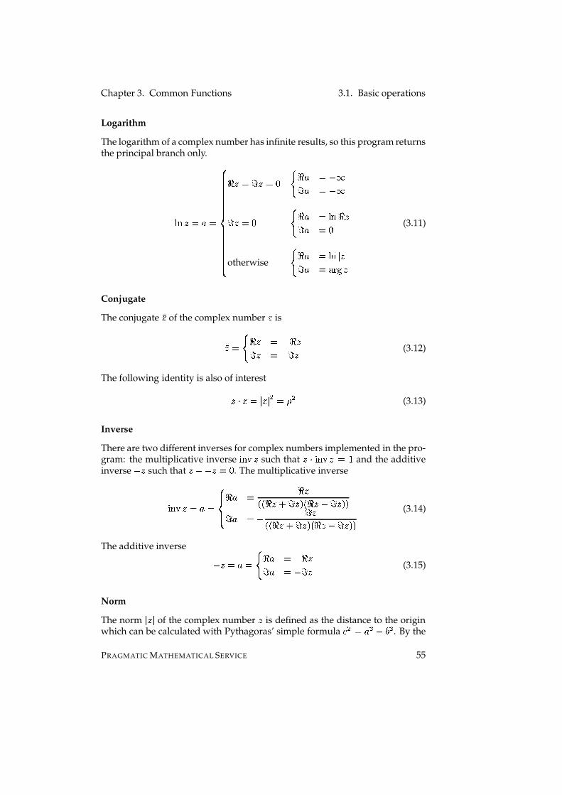
Chapter 3. Common Functions 3.1. Basic operations
Logarithm
The logarithm of a complex number has infinite results, so this program returnsthe principal branch only.
�5 �ÆÕI«9ËI ¹ººººººººººººº» ººººººººººººº¼
ʱÆÇI ÌSÆÇIL� _ ʱ9 Ièw gÌS9 Ièw gÌSÆÇI¶� _ ʱ9 I �� �ʱÆÌS9 I¶�otherwise _ ʱ9 I �� Õà Æ�àÌS9 I¶�jW�^}Æ
(3.11)
Conjugate
The conjugate �Æ of the complex number Æ is�ÆÕI _ 汮 I ʱÆÌSÆ IÍwÁÌSÆ (3.12)
The following identity is also of interestÆ~ëU�ÆÕI à Æöà $ I � $ (3.13)
Inverse
There are two different inverses for complex numbers implemented in the pro-gram: the multiplicative inverse 35 9�²Æ such that ÆËë�3� 9�²Æ©I ) and the additiveinverse w�Æ such that Æ�rLw�ÆÕI«� . The multiplicative inverse
35 9�²ÆÕI¶9�I ¹º» º¼Ê±9 I ʱÆ���zʱÆÁrtÌSÆ��<�zʱÆ,w¬ÌSÆ��4�ÌS9 Ièw ÌSÆ�4�qʱÆsrtÌSÆ��<�zʱÆ6w¬ÌSÆ��4� (3.14)
The additive inverse w�Æ6I«9ËI _ ʱ9 Ièw�ʱÆÌS9 IèwÁÌSÆ (3.15)
Norm
The norm à Æöà of the complex number Æ is defined as the distance to the originwhich can be calculated with Pythagoras’ simple formula u $ I 9 $ r�; $ . By the
PRAGMATIC MATHEMATICAL SERVICE 55
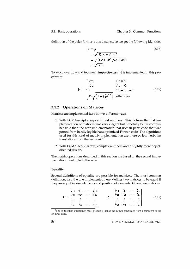
3.1. Basic operations Chapter 3. Common Functions
definition of the polar form � is this distance, so we get the following identitiesà Æ�à�I � (3.16)I �zʱÆ�� $ r¶�ÞÌSÆ�� $I �zʱÆÁr�ÌSÆ����qʱÆ,wvÌSÆ��I . Æ,ë(�ÆTo avoid overflow and too much impreciseness à Æ�à is implemented in this pro-gram as
à Æöà�I ¹ººººº» ººººº¼à ʱÆ�à ÌSÆÕI«�à ÌSÆ�à ʱÆÕI«�� ʱÆÕI ÌSÆÕI«�汮 \ 1()xr u � D� D w $ 2 otherwise
(3.17)
3.1.2 Operations on Matrices
Matrices are implemented here in two different ways:
1. With ECMA-script arrays and real numbers. This is from the first im-plementation of matrices, not very elegant but hopefully better compre-hensible than the new implementation that uses in parts code that wasported from hardly legible handoptimized Fortran code. The algorithmsused for this kind of matrix implementation are more or less verbatimtranslations from the textbook2.
2. With ECMA-script arrays, complex numbers and a slightly more object-oriented design.
The matrix operations described in this section are based on the second imple-mentation if not noted otherwise.
Equality
Several definitions of equality are possible for matrices. The most commondefinition, also the one implemented here, defines two matrices to be equal ifthey are equal in size, elements and position of elements. Given two matricesp I � ¡
9 "�" 9 " $ ����� 9 " �9 $ " 9 $�$ ����� 9 $ �...
.... . .
...9 � " 9 � $ ����� 9 ���¤ ¥¥¥§ � I � ¡
; "�" ; " $ ����� ; "��; $ " ; $�$ ����� ; $ �......
. . ....; ï " ; ï $ ����� ; ï �¤ ¥¥¥§ (3.18)
2The textbook in question is most probably [25] as the author concludes from a comment in theoriginal code.
56 PRAGMATIC MATHEMATICAL SERVICE

Chapter 3. Common Functions 3.1. Basic operations
these matrices are equal in size, elements and position of elements ifp I ������� 9 �^� � p�� ; ï � � � k�; ï � à 9 �^� I«; ï � 1Ç�2I¶ò�1 ½ I$#j15k³��: ½ :�òö:�# l �VW l(3.19)The equation 3.19 is simplified—matrices are not common sets of course—butbasically correct3.
Addition
The addition of two matrices of the same size and form is done by adding theelements of the same positions.p r � I � ¡
9 "�" rn; "�" 9 " $ rt; " $ ����� 9 " � rt; "��9 $ " rn; $ " 9 $�$ rt; $�$ ����� 9 $ � rt; $ �......
. . ....9 � " rt; ï " 9 � $ rt; ï $ ����� 9 ��� rn; ï �
¤¦¥¥¥§ (3.20)
Subtraction
The subtraction of two matrices is implemented by multiplying one matrixwith w6) and adding both. p w � I p r«� � ë��°w6)´�4� (3.21)
Multiplication
The multiplication of two matrices is a bit more complicated.
matrix
ptimes a number � That is the simplest algorithm in this group: just
multiply every element with the number.p ë<�iIÎ� ¡9 "�" ë<� 9 " $ ë<� ����� 9 " � ë��9 $ " ë<� 9 $�$ ë<� ����� 9 $ � ë��
......
. . ....9 � " ë<� 9 � $ ë<� ����� 9 �^� ë<�¤¦¥¥¥§ (3.22)
matrix
ptimes matrix
�The product of two matrices is only defined if
½ I ò ,that is if
phas as many columns as
�has rows. The algorithm itself is
nearly as simple as matrix addition.
u � � I ��C � " 9 � C ; C � (3.23)
3Hopes the author.
PRAGMATIC MATHEMATICAL SERVICE 57

3.1. Basic operations Chapter 3. Common Functions
Example: p I � 9 "�" 9 " $ 9 " ê9 $ " 9 $�$ 9 $ ê �� I �¡ ; "�" ; " $; $ " ; $�$; ê " ; ê $
¤§ (3.24)/ I p � (3.25)u "�" I¶9 "�" ;´)!)}rn9 " $ ; / )}rv9 " ê ;���) (3.26)u " $ I¶9 "�" ;´) / rn9 " $ ; /!/ rv9 " ê ;�� / (3.27)u $ " I¶9 $ " ;´)!)}rn9 $�$ ; / )}rv9 $ ê ;���) (3.28)u $�$ I¶9 $�$ ;´) / rn9 $�$ ; /!/ rv9 $ ê ;�� / (3.29)
Matrix multiplication is not commutative!p � HI � p for most
p : � (3.30)
Example: p I � ) /� � � � I � / ))¢ó´� (3.31)p � I � � )!))³� / �´� (3.32)� p I � ó õ) ì /!/ � (3.33)
The conditions such that
p � I � p are� if both matrices are equal under the conditions described in equation 3.19� if all elements of one or both of two square matrices are zero� if the size of at least one matrix is one (only one element)
Division
The division of two matrices)W is implemented as the product of
pand the
inverse of
�. For an explanation of the matrix inverse see 26
Rotation
One of the sometimes ridiculed but nevertheless useful operations is the rota-tion of the matrix 90 degrees anti-clockwise.W�&�� : ? � 9 "�" 9 " $ 9 " ê9 $ " 9 $�$ 9 $ ê � I �¡ 9 " ê 9 $ ê9 " $ 9 $�$9 "�" 9 $ "
¤§ (3.34)
58 PRAGMATIC MATHEMATICAL SERVICE

Chapter 3. Common Functions 3.1. Basic operations
Main Diagonal
The main diagonal of a matrix is described for a square matrix bya 35�,^�� p �}I k³9 "�" :�9 $�$ : ����� :�9 �5� l (3.35)
Trace
The trace is the sum of the elements on the main diagonal. For a �#T©� matrixp
it is defined as ��W��(%�ã!� p �}I«9 "�" rn9 $�$ rn9 ê�ê (3.36)
Norm, 2-Norm, Rank
These values are calculated by doing a singular value decomposition of thematrix. The singular value decomposition is sadly implemented for real matri-ces only. The 2-norm of a matrix is sometimes called the condition and notatedin equations for a matrix
pas %<&( a � p �
Determinant
The determinant for square matrices is determined differently depending onthe size of the matrix.)6Te) The determinant of a constant is the constant itself/ T / Direct way a ã��³� p �}I«9 "�" 9 $�$ wy9 " $ 9 $ " (3.37)��TV� By following Sarrus’ rule strictlya ã<�³� p �}I«9 "�" 9 $�$ 9 ê�ê (3.38)rn9 " $ 9 $ ê 9 ê " (3.39)rn9 " ê 9 $ " 9 ê $ (3.40)wy9 " ê 9 $�$ 9 ê " (3.41)wy9 " $ 9 $ " 9 ê�ê (3.42)wy9 "�" 9 $ ê 9 ê $ (3.43)�eT¸� with �G(Ô� This is done by means of the LU-decomposition in the new
implementation of matrices and by building and adding all subdetermi-nants in a computationaly very expensive recursion in the old one.
For further explanations see the chapter about linear algebra on page 97.
PRAGMATIC MATHEMATICAL SERVICE 59
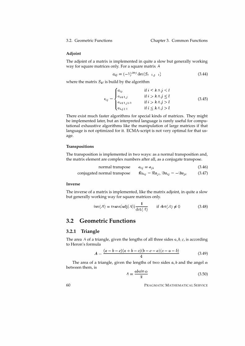
3.2. Geometric Functions Chapter 3. Common Functions
Adjoint
The adjoint of a matrix is implemented in quite a slow but generally workingway for square matrices only. For a square matrix
p9 ��� IN�4w6)³� �5��� a ã��³�q1 ��® " ® �<® " � (3.44)
where the matrix 1 ï � is build by the algorithm
' ��� I ¹ººº» ººº¼9 �^� if �v�Lò�1 ½ ��#9 ��� " ® � if �v(Lò�1 ½ ��#9 ��� " ® ��� " if �v(Lò�1 ½ (�#9 �V® ��� " if �v�Lò�1 ½ (�# (3.45)
There exist much faster algorithms for special kinds of matrices. They mightbe implemented later, but an interpreted language is rarely useful for compu-tational exhaustive algorithms like the manipulation of large matrices if thatlanguage is not optimized for it. ECMA-script is not very optimal for that us-age.
Transpositions
The transposition is implemented in two ways: as a normal transposition and,the matrix element are complex numbers after all, as a conjugate transpose.
normal transpose 9 ��� I¶9 ��� (3.46)conjugated normal transpose ʱ9 ��� I«Ê±9 ��� :�ÌS9 �^� IèwÁÌS9 ��� (3.47)
Inverse
The inverse of a matrix is implemented, like the matrix adjoint, in quite a slowbut generally working way for square matrices only.3� 9��� p �}IL�3W_�� �'���� a�� � p ��� )a ã���� p � if a ã<��� p � HIL� (3.48)
3.2 Geometric Functions
3.2.1 Triangle
The area
pof a triangle, given the lengths of all three sides 9:_;´:�u , is according
to Heron’s formulap I �q9srt;@rvu�����96rn;xwyu��<�z;{rvuSwy9|�<��u}rn9~wv;<�� (3.49)
The area of a triangle, given the lengths of two sides 9�:�; and the angel �between them, is
p I 9|;ö'�3� �/ (3.50)
60 PRAGMATIC MATHEMATICAL SERVICE
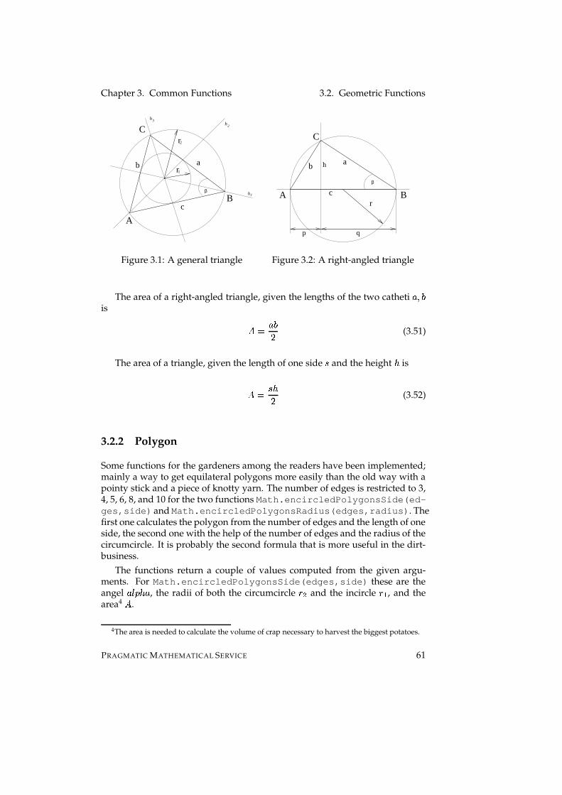
Chapter 3. Common Functions 3.2. Geometric Functions
B
A
C
a
c
b r1
2r
β
hh
1
2
3
h
Figure 3.1: A general triangle
A
C
r
β
Bc
b a
p q
h
Figure 3.2: A right-angled triangle
The area of a right-angled triangle, given the lengths of the two catheti 9�:_;is p I 9|;/ (3.51)
The area of a triangle, given the length of one side ' and the height D isp I 'fD/ (3.52)
3.2.2 Polygon
Some functions for the gardeners among the readers have been implemented;mainly a way to get equilateral polygons more easily than the old way with apointy stick and a piece of knotty yarn. The number of edges is restricted to 3,4, 5, 6, 8, and 10 for the two functions Math.encircledPolygonsSide(ed-ges,side) and Math.encircledPolygonsRadius(edges,radius). Thefirst one calculates the polygon from the number of edges and the length of oneside, the second one with the help of the number of edges and the radius of thecircumcircle. It is probably the second formula that is more useful in the dirt-business.
The functions return a couple of values computed from the given argu-ments. For Math.encircledPolygonsSide(edges,side) these are theangel 9S# � D9 , the radii of both the circumcircle * $ and the incircle * " , and thearea4
p.
4The area is needed to calculate the volume of crap necessary to harvest the biggest potatoes.
PRAGMATIC MATHEMATICAL SERVICE 61
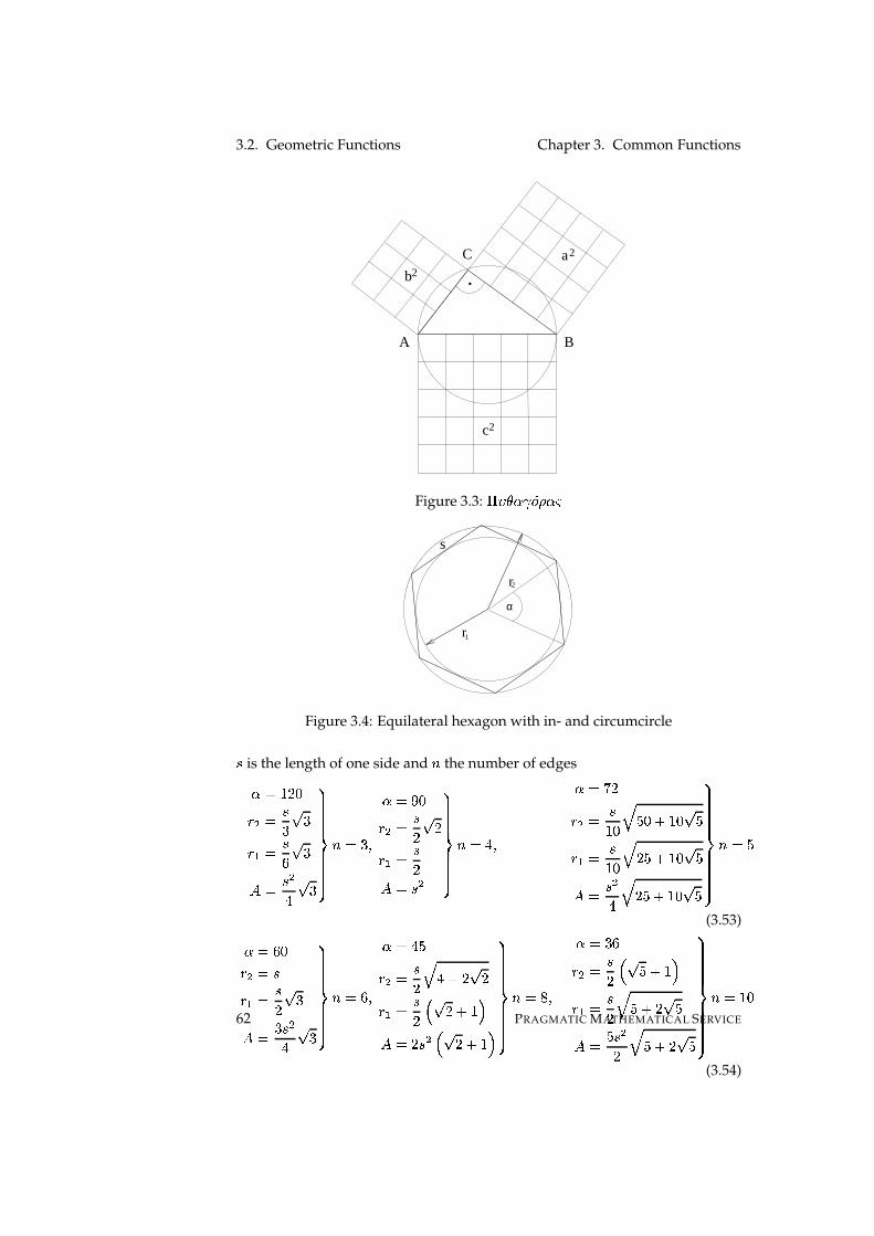
3.2. Geometric Functions Chapter 3. Common Functions
b
BA
C
.2
a
c
2
2
Figure 3.3: ����Ñ �å����������r2
r1
s
α
Figure 3.4: Equilateral hexagon with in- and circumcircle' is the length of one side and � the number of edges� IN) / �* $ I '� . �* " I 'ì . �p I ' $� . �� ººººººº�ººººººº��iI«�7:
� IL�(�* $ I '/ . /* " I '/p I¬' $� ºººººº�ºººººº� �©I
� :� I í /* $ I ')�� « ó���r¶)�� . ó* " I ')�� « / ó²r¶)�� . óp I ' $� « / ó²r¶)³� . ó
� ºººººººº�ºººººººº��©I¶ó
(3.53)� I ì �* $ Io'* " I '/ . �p I ��' $� . �� ºººººº�ºººººº� �iI
ì :� I � ó* $ I '/ « � r / . /* " I '/ 1 . / r¶) 2p I / ' $ 1 . / r¶) 2
� ººººººº�ººººººº��iI«õ7:
� I«� ì* $ I '/ 1 . ó�rL) 2* " I '/ « ó�r / . óp I ó$' $/ « ó�r / . ó� ºººººººº�ºººººººº��iIN)��
(3.54)
62 PRAGMATIC MATHEMATICAL SERVICE

Chapter 3. Common Functions 3.2. Geometric Functionsu is the circumference of the polygon� IN) / �'ÁI * $ . �u²I«� * $ . �* " I * $/p I � * $$� . �� ººººººººº�ººººººººº��iI¶��:
� I«�!�'ÁI * $ . /u²I � * $ . /* " I * $/ . /p I / * $$� ºººººººº�ºººººººº��iI � :
� I í /'ÁI * $/ « )��,w / . óu�I ó * $/ « )³�sw / . ó* " I * $� 1 . ó�r¶)F2p I ó * $õ « )³��r / . / �� ºººººººººººº�ºººººººººººº��VI ó
(3.55)� I ì �'sI * $u�I ì * $* " I * $/ . �p I � * $/ . �� ºººººººº�ºººººººº��iI ì :
� I � ó'ÁI * $ « / w . /u²I«õ * $ « / w . /* " I * $/ « / r . /p I / * $$ . /� ºººººººººº�ºººººººººº��©I¶õ�:
� I«� ì'ÁI * $/ 1 . ósw�) 2u�I ó * $ 1 . ósw�)F2* " I * $�b« )���r / . óp I ó * $� « )³�sw / . ó� ºººººººººººº�ºººººººººººº��©Iè)³�
(3.56)
A couple of more general formulas for equilateral polygons are also imple-mented. u�IÔ� * $ '�3� .1 �� 2 (3.57)u�I / � * " �_�� 1 �� 2 (3.58)p IÔ� * $$ '�35 ©ð / ��vñ )/ (3.59)p IÔ� * $" �_�� 1 � � 2 (3.60)'sI / * $ '�3� ©ð / �� ñ (3.61)
3.2.3 Circle
“Circle” is the common name of the set of all points with the same distancefrom a fixed point u . The following formulas are for a circle on a plane.
Circumference
The circumference ç of a circle can be calculated in a lot of ways. One of thesepaths is ç I / * � (3.62)
PRAGMATIC MATHEMATICAL SERVICE 63
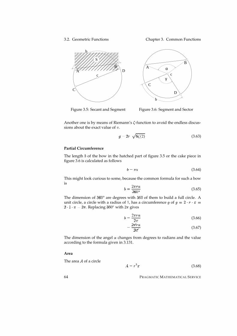
3.2. Geometric Functions Chapter 3. Common Functions
�,�,�,�,�,�,�,�,�,�,�,�,�,�,�,�,�,�,�,�,�,��,�,�,�,�,�,�,�,�,�,�,�,�,�,�,�,�,�,�,�,�,��,�,�,�,�,�,�,�,�,�,�,�,�,�,�,�,�,�,�,�,�,��,�,�,�,�,�,�,�,�,�,�,�,�,�,�,�,�,�,�,�,�,��,�,�,�,�,�,�,�,�,�,�,�,�,�,�,�,�,�,�,�,�,��,�,�,�,�,�,�,�,�,�,�,�,�,�,�,�,�,�,�,�,�,��,�,�,�,�,�,�,�,�,�,�,�,�,�,�,�,�,�,�,�,�,��,�,�,�,�,�,�,�,�,�,�,�,�,�,�,�,�,�,�,�,�,��,�,�,�,�,�,�,�,�,�,�,�,�,�,�,�,�,�,�,�,�,��,�,�,�,�,�,�,�,�,�,�,�,�,�,�,�,�,�,�,�,�,��,�,�,�,�,�,�,�,�,�,�,�,�,�,�,�,�,�,�,�,�,��,�,�,�,�,�,�,�,�,�,�,�,�,�,�,�,�,�,�,�,�,��,�,�,�,�,�,�,�,�,�,�,�,�,�,�,�,�,�,�,�,�,��,�,�,�,�,�,�,�,�,�,�,�,�,�,�,�,�,�,�,�,�,��,�,�,�,�,�,�,�,�,�,�,�,�,�,�,�,�,�,�,�,�,��,�,�,�,�,�,�,�,�,�,�,�,�,�,�,�,�,�,�,�,�,��,�,�,�,�,�,�,�,�,�,�,�,�,�,�,�,�,�,�,�,�,��,�,�,�,�,�,�,�,�,�,�,�,�,�,�,�,�,�,�,�,�,�A
S
BD
C
c
b
Figure 3.5: Secant and Segment
AB
C
D
b
c
α
γ
Figure 3.6: Segment and Sector
Another one is by means of Riemann’s � -function to avoid the endless discus-sions about the exact value of � .ç I / * ��� ì �7�
/ � ��� (3.63)
Partial Circumference
The length ; of the bow in the hatched part of figure 3.5 or the cake piece infigure 3.6 is calculated as follows ;²I * � (3.64)
This might look curious to some, because the common formula for such a bowis ;²I / � * �� ì �S (3.65)
The dimension of � ì � are degrees with � ì � of them to build a full circle. Aunit circle, a circle with a radius of ) , has a circumference ç of ç I / ë * ë � I/ ë�)²ë � I / � . Replacing � ì � with
/ � gives;²I / � * �/ � (3.66)I�¡ ¡/ � * �¡ ¡/ � (3.67)
The dimension of the angel � changes from degrees to radians and the valueaccording to the formula given in 3.131.
Area
The area
pof a circle
p I * $ � (3.68)
64 PRAGMATIC MATHEMATICAL SERVICE
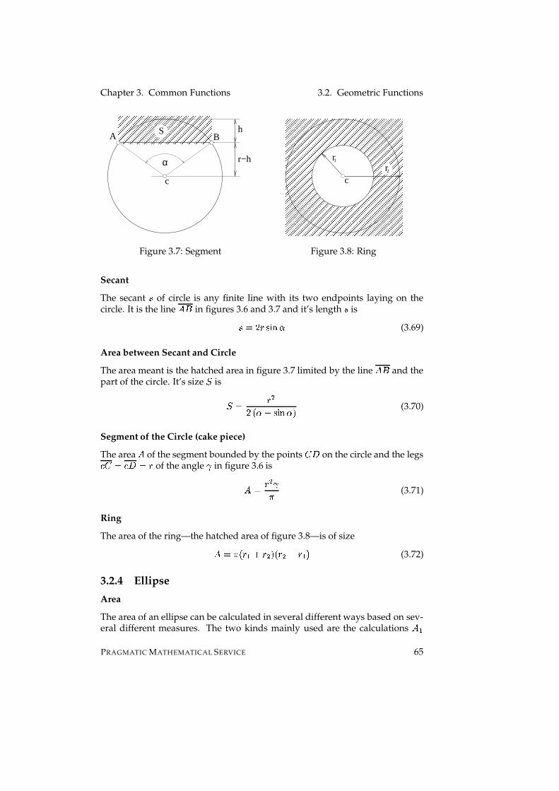
Chapter 3. Common Functions 3.2. Geometric Functions
¢,¢,¢,¢,¢,¢,¢,¢,¢,¢,¢,¢,¢,¢,¢,¢,¢,¢,¢,¢¢,¢,¢,¢,¢,¢,¢,¢,¢,¢,¢,¢,¢,¢,¢,¢,¢,¢,¢,¢¢,¢,¢,¢,¢,¢,¢,¢,¢,¢,¢,¢,¢,¢,¢,¢,¢,¢,¢,¢¢,¢,¢,¢,¢,¢,¢,¢,¢,¢,¢,¢,¢,¢,¢,¢,¢,¢,¢,¢¢,¢,¢,¢,¢,¢,¢,¢,¢,¢,¢,¢,¢,¢,¢,¢,¢,¢,¢,¢¢,¢,¢,¢,¢,¢,¢,¢,¢,¢,¢,¢,¢,¢,¢,¢,¢,¢,¢,¢£,£,£,£,£,£,£,£,£,£,£,£,£,£,£,£,£,£,£,££,£,£,£,£,£,£,£,£,£,£,£,£,£,£,£,£,£,£,££,£,£,£,£,£,£,£,£,£,£,£,£,£,£,£,£,£,£,££,£,£,£,£,£,£,£,£,£,£,£,£,£,£,£,£,£,£,££,£,£,£,£,£,£,£,£,£,£,£,£,£,£,£,£,£,£,££,£,£,£,£,£,£,£,£,£,£,£,£,£,£,£,£,£,£,£α
c
BAh
r−h
S
Figure 3.7: Segment ¤,¤,¤,¤,¤,¤,¤,¤,¤,¤,¤,¤,¤,¤,¤,¤,¤,¤,¤,¤,¤,¤,¤,¤,¤¤,¤,¤,¤,¤,¤,¤,¤,¤,¤,¤,¤,¤,¤,¤,¤,¤,¤,¤,¤,¤,¤,¤,¤,¤¤,¤,¤,¤,¤,¤,¤,¤,¤,¤,¤,¤,¤,¤,¤,¤,¤,¤,¤,¤,¤,¤,¤,¤,¤¤,¤,¤,¤,¤,¤,¤,¤,¤,¤,¤,¤,¤,¤,¤,¤,¤,¤,¤,¤,¤,¤,¤,¤,¤¤,¤,¤,¤,¤,¤,¤,¤,¤,¤,¤,¤,¤,¤,¤,¤,¤,¤,¤,¤,¤,¤,¤,¤,¤¤,¤,¤,¤,¤,¤,¤,¤,¤,¤,¤,¤,¤,¤,¤,¤,¤,¤,¤,¤,¤,¤,¤,¤,¤¤,¤,¤,¤,¤,¤,¤,¤,¤,¤,¤,¤,¤,¤,¤,¤,¤,¤,¤,¤,¤,¤,¤,¤,¤¤,¤,¤,¤,¤,¤,¤,¤,¤,¤,¤,¤,¤,¤,¤,¤,¤,¤,¤,¤,¤,¤,¤,¤,¤¤,¤,¤,¤,¤,¤,¤,¤,¤,¤,¤,¤,¤,¤,¤,¤,¤,¤,¤,¤,¤,¤,¤,¤,¤¤,¤,¤,¤,¤,¤,¤,¤,¤,¤,¤,¤,¤,¤,¤,¤,¤,¤,¤,¤,¤,¤,¤,¤,¤¤,¤,¤,¤,¤,¤,¤,¤,¤,¤,¤,¤,¤,¤,¤,¤,¤,¤,¤,¤,¤,¤,¤,¤,¤¤,¤,¤,¤,¤,¤,¤,¤,¤,¤,¤,¤,¤,¤,¤,¤,¤,¤,¤,¤,¤,¤,¤,¤,¤¤,¤,¤,¤,¤,¤,¤,¤,¤,¤,¤,¤,¤,¤,¤,¤,¤,¤,¤,¤,¤,¤,¤,¤,¤¤,¤,¤,¤,¤,¤,¤,¤,¤,¤,¤,¤,¤,¤,¤,¤,¤,¤,¤,¤,¤,¤,¤,¤,¤¤,¤,¤,¤,¤,¤,¤,¤,¤,¤,¤,¤,¤,¤,¤,¤,¤,¤,¤,¤,¤,¤,¤,¤,¤¤,¤,¤,¤,¤,¤,¤,¤,¤,¤,¤,¤,¤,¤,¤,¤,¤,¤,¤,¤,¤,¤,¤,¤,¤¤,¤,¤,¤,¤,¤,¤,¤,¤,¤,¤,¤,¤,¤,¤,¤,¤,¤,¤,¤,¤,¤,¤,¤,¤¤,¤,¤,¤,¤,¤,¤,¤,¤,¤,¤,¤,¤,¤,¤,¤,¤,¤,¤,¤,¤,¤,¤,¤,¤¤,¤,¤,¤,¤,¤,¤,¤,¤,¤,¤,¤,¤,¤,¤,¤,¤,¤,¤,¤,¤,¤,¤,¤,¤¤,¤,¤,¤,¤,¤,¤,¤,¤,¤,¤,¤,¤,¤,¤,¤,¤,¤,¤,¤,¤,¤,¤,¤,¤¤,¤,¤,¤,¤,¤,¤,¤,¤,¤,¤,¤,¤,¤,¤,¤,¤,¤,¤,¤,¤,¤,¤,¤,¤¤,¤,¤,¤,¤,¤,¤,¤,¤,¤,¤,¤,¤,¤,¤,¤,¤,¤,¤,¤,¤,¤,¤,¤,¤¤,¤,¤,¤,¤,¤,¤,¤,¤,¤,¤,¤,¤,¤,¤,¤,¤,¤,¤,¤,¤,¤,¤,¤,¤¤,¤,¤,¤,¤,¤,¤,¤,¤,¤,¤,¤,¤,¤,¤,¤,¤,¤,¤,¤,¤,¤,¤,¤,¤¤,¤,¤,¤,¤,¤,¤,¤,¤,¤,¤,¤,¤,¤,¤,¤,¤,¤,¤,¤,¤,¤,¤,¤,¤¥,¥,¥,¥,¥,¥,¥,¥,¥,¥,¥,¥,¥,¥,¥,¥,¥,¥,¥,¥,¥,¥,¥,¥,¥¥,¥,¥,¥,¥,¥,¥,¥,¥,¥,¥,¥,¥,¥,¥,¥,¥,¥,¥,¥,¥,¥,¥,¥,¥¥,¥,¥,¥,¥,¥,¥,¥,¥,¥,¥,¥,¥,¥,¥,¥,¥,¥,¥,¥,¥,¥,¥,¥,¥¥,¥,¥,¥,¥,¥,¥,¥,¥,¥,¥,¥,¥,¥,¥,¥,¥,¥,¥,¥,¥,¥,¥,¥,¥¥,¥,¥,¥,¥,¥,¥,¥,¥,¥,¥,¥,¥,¥,¥,¥,¥,¥,¥,¥,¥,¥,¥,¥,¥¥,¥,¥,¥,¥,¥,¥,¥,¥,¥,¥,¥,¥,¥,¥,¥,¥,¥,¥,¥,¥,¥,¥,¥,¥¥,¥,¥,¥,¥,¥,¥,¥,¥,¥,¥,¥,¥,¥,¥,¥,¥,¥,¥,¥,¥,¥,¥,¥,¥¥,¥,¥,¥,¥,¥,¥,¥,¥,¥,¥,¥,¥,¥,¥,¥,¥,¥,¥,¥,¥,¥,¥,¥,¥¥,¥,¥,¥,¥,¥,¥,¥,¥,¥,¥,¥,¥,¥,¥,¥,¥,¥,¥,¥,¥,¥,¥,¥,¥¥,¥,¥,¥,¥,¥,¥,¥,¥,¥,¥,¥,¥,¥,¥,¥,¥,¥,¥,¥,¥,¥,¥,¥,¥¥,¥,¥,¥,¥,¥,¥,¥,¥,¥,¥,¥,¥,¥,¥,¥,¥,¥,¥,¥,¥,¥,¥,¥,¥¥,¥,¥,¥,¥,¥,¥,¥,¥,¥,¥,¥,¥,¥,¥,¥,¥,¥,¥,¥,¥,¥,¥,¥,¥¥,¥,¥,¥,¥,¥,¥,¥,¥,¥,¥,¥,¥,¥,¥,¥,¥,¥,¥,¥,¥,¥,¥,¥,¥¥,¥,¥,¥,¥,¥,¥,¥,¥,¥,¥,¥,¥,¥,¥,¥,¥,¥,¥,¥,¥,¥,¥,¥,¥¥,¥,¥,¥,¥,¥,¥,¥,¥,¥,¥,¥,¥,¥,¥,¥,¥,¥,¥,¥,¥,¥,¥,¥,¥¥,¥,¥,¥,¥,¥,¥,¥,¥,¥,¥,¥,¥,¥,¥,¥,¥,¥,¥,¥,¥,¥,¥,¥,¥¥,¥,¥,¥,¥,¥,¥,¥,¥,¥,¥,¥,¥,¥,¥,¥,¥,¥,¥,¥,¥,¥,¥,¥,¥¥,¥,¥,¥,¥,¥,¥,¥,¥,¥,¥,¥,¥,¥,¥,¥,¥,¥,¥,¥,¥,¥,¥,¥,¥¥,¥,¥,¥,¥,¥,¥,¥,¥,¥,¥,¥,¥,¥,¥,¥,¥,¥,¥,¥,¥,¥,¥,¥,¥¥,¥,¥,¥,¥,¥,¥,¥,¥,¥,¥,¥,¥,¥,¥,¥,¥,¥,¥,¥,¥,¥,¥,¥,¥¥,¥,¥,¥,¥,¥,¥,¥,¥,¥,¥,¥,¥,¥,¥,¥,¥,¥,¥,¥,¥,¥,¥,¥,¥¥,¥,¥,¥,¥,¥,¥,¥,¥,¥,¥,¥,¥,¥,¥,¥,¥,¥,¥,¥,¥,¥,¥,¥,¥¥,¥,¥,¥,¥,¥,¥,¥,¥,¥,¥,¥,¥,¥,¥,¥,¥,¥,¥,¥,¥,¥,¥,¥,¥¥,¥,¥,¥,¥,¥,¥,¥,¥,¥,¥,¥,¥,¥,¥,¥,¥,¥,¥,¥,¥,¥,¥,¥,¥¥,¥,¥,¥,¥,¥,¥,¥,¥,¥,¥,¥,¥,¥,¥,¥,¥,¥,¥,¥,¥,¥,¥,¥,¥
c
rr2
1
Figure 3.8: Ring
Secant
The secant ' of circle is any finite line with its two endpoints laying on thecircle. It is the line
p �in figures 3.6 and 3.7 and it’s length ' is'sI / * '�3� � (3.69)
Area between Secant and Circle
The area meant is the hatched area in figure 3.7 limited by the line
p �and the
part of the circle. It’s size 1 is 1eI * $/ � � we'�3� � � (3.70)
Segment of the Circle (cake piece)
The area
pof the segment bounded by the points
/§¦on the circle and the legsu / I u ¦ I * of the angle � in figure 3.6 isp I * $ �� (3.71)
Ring
The area of the ring—the hatched area of figure 3.8—is of sizep I � � * " r * $ ��� * $ w * " � (3.72)
3.2.4 Ellipse
Area
The area of an ellipse can be calculated in several different ways based on sev-eral different measures. The two kinds mainly used are the calculations
p "PRAGMATIC MATHEMATICAL SERVICE 65
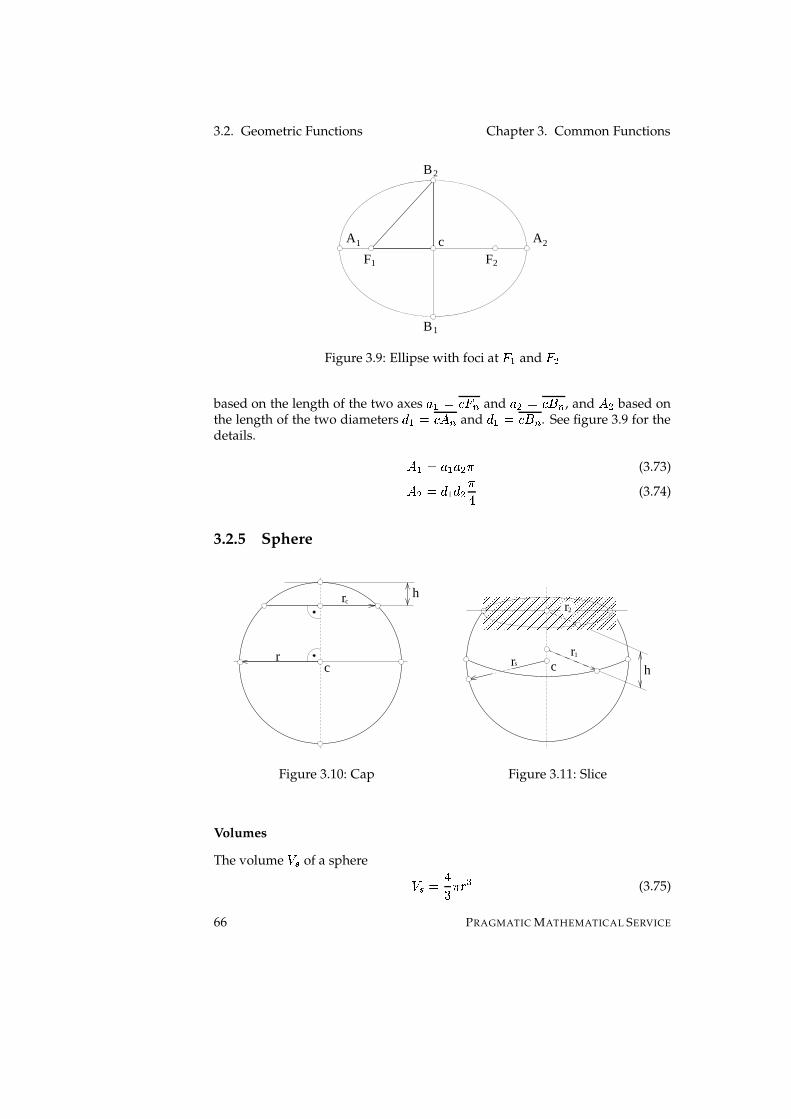
3.2. Geometric Functions Chapter 3. Common Functions
A A
F F
B
1
1
1
B2
2
2
c
Figure 3.9: Ellipse with foci at t " and t $based on the length of the two axes 9 " I u�t C and 9 $ I u � C , and
p $ based onthe length of the two diameters j " I u
p C and j " I u� C . See figure 3.9 for the
details. p " I¶9 " 9 $ � (3.73)p $ I j " j $ � � (3.74)
3.2.5 Sphere
rc
hcr
Figure 3.10: Cap
c h
r1sr
¨,¨,¨,¨,¨,¨,¨,¨,¨,¨,¨,¨,¨,¨,¨,¨,¨,¨,¨,¨¨,¨,¨,¨,¨,¨,¨,¨,¨,¨,¨,¨,¨,¨,¨,¨,¨,¨,¨,¨¨,¨,¨,¨,¨,¨,¨,¨,¨,¨,¨,¨,¨,¨,¨,¨,¨,¨,¨,¨¨,¨,¨,¨,¨,¨,¨,¨,¨,¨,¨,¨,¨,¨,¨,¨,¨,¨,¨,¨¨,¨,¨,¨,¨,¨,¨,¨,¨,¨,¨,¨,¨,¨,¨,¨,¨,¨,¨,¨©,©,©,©,©,©,©,©,©,©,©,©,©,©,©,©,©,©,©,©©,©,©,©,©,©,©,©,©,©,©,©,©,©,©,©,©,©,©,©©,©,©,©,©,©,©,©,©,©,©,©,©,©,©,©,©,©,©,©©,©,©,©,©,©,©,©,©,©,©,©,©,©,©,©,©,©,©,©©,©,©,©,©,©,©,©,©,©,©,©,©,©,©,©,©,©,©,©r2
Figure 3.11: Slice
Volumes
The volume ª @ of a sphere ª @ I � � � * ê (3.75)
66 PRAGMATIC MATHEMATICAL SERVICE

Chapter 3. Common Functions 3.2. Geometric Functions
The volume ª¬« of a cap of a sphere (figure: 3.10)ª¬«xI D �ì u � * $« r�D $ w (3.76)I D $ �� �q� * wD�� (3.77)
Areas
The area
pof a sphere
p I � � * $ (3.78)
3.2.6 Torus
®,®,®,®,®,®,®,®,®,®,®®,®,®,®,®,®,®,®,®,®,®®,®,®,®,®,®,®,®,®,®,®®,®,®,®,®,®,®,®,®,®,®®,®,®,®,®,®,®,®,®,®,®®,®,®,®,®,®,®,®,®,®,®¯,¯,¯,¯,¯,¯,¯,¯,¯,¯¯,¯,¯,¯,¯,¯,¯,¯,¯,¯¯,¯,¯,¯,¯,¯,¯,¯,¯,¯¯,¯,¯,¯,¯,¯,¯,¯,¯,¯¯,¯,¯,¯,¯,¯,¯,¯,¯,¯¯,¯,¯,¯,¯,¯,¯,¯,¯,¯°,°,°,°,°,°,°,°,°,°°,°,°,°,°,°,°,°,°,°°,°,°,°,°,°,°,°,°,°°,°,°,°,°,°,°,°,°,°°,°,°,°,°,°,°,°,°,°°,°,°,°,°,°,°,°,°,°±,±,±,±,±,±,±,±,±,±±,±,±,±,±,±,±,±,±,±±,±,±,±,±,±,±,±,±,±±,±,±,±,±,±,±,±,±,±±,±,±,±,±,±,±,±,±,±±,±,±,±,±,±,±,±,±,±rr1 2
Figure 3.12: Torus
The Volume ª of a torus ªèI / � $ * $" * $ (3.79)
The area
pof a torus
p I � � $ * " * $ (3.80)
3.2.7 Cone
The cones here are always cones with a circle as the base.
Volume
The volume ª of a slanted cone (figure: 3.14)ªNI )� � * $ D (3.81)
The mantel area
p E of a straight cone (figure: 3.13)p E I � * ' (3.82)
PRAGMATIC MATHEMATICAL SERVICE 67

3.2. Geometric Functions Chapter 3. Common Functions
²³²³²³²³²³²³²³²³²³²³²³²³²³²²³²³²³²³²³²³²³²³²³²³²³²³²³²²³²³²³²³²³²³²³²³²³²³²³²³²³²´³´³´³´³´³´³´³´³´³´³´³´³´³´´³´³´³´³´³´³´³´³´³´³´³´³´³´´³´³´³´³´³´³´³´³´³´³´³´³´³´hs
r
Figure 3.13: A straight cone µ³µ³µ³µ³µ³µ³µ³µ³µ³µ³µ³µ³µ³µµ³µ³µ³µ³µ³µ³µ³µ³µ³µ³µ³µ³µ³µµ³µ³µ³µ³µ³µ³µ³µ³µ³µ³µ³µ³µ³µ¶³¶³¶³¶³¶³¶³¶³¶³¶³¶³¶³¶³¶³¶¶³¶³¶³¶³¶³¶³¶³¶³¶³¶³¶³¶³¶³¶¶³¶³¶³¶³¶³¶³¶³¶³¶³¶³¶³¶³¶³¶r
h3
h2
h1 c
c3
c2
1
Figure 3.14: Three slanted cones
The area
pof a straight cone (figure: 3.13)p I p «}ë p E (3.83)I * $ � ë � * ' (3.84)I * ê � ê ' (3.85)
The side ' of a straight cone (figure: 3.13)'ÁI * $ r�D $ (3.86)
The height D of a straight cone (figure: 3.13)D#I ' $ w * $ (3.87)
3.2.8 Miscellaneous Geometric Figures
Lame Curve
The gnuplot script to produce figure 3.15 was: �1 s e t terminal f i g big f o n t s i z e 12 metric ;2 s e t output ” s u p e r e l l i p s e . f i g ” ;3 s e t parametric ;4 s e t trange [ � 2 � pi : 2 � pi ] ;5 s e t xrange [ � 3 . 2 : 3 . 2 ] ; s e t yrange [ � 3 . 2 : 3 . 2 ] ;6 y ( t , n ) =b � sgn ( sin ( t ) ) � abs ( sin ( t ) ) �|� (2/n ) ;7 x ( t , n ) =a � sgn ( cos ( t ) ) � abs ( cos ( t ) ) �|� (2/n ) ;8 a =2; b =3; plot s9 x ( t , 3 ) , y ( t , 3 ) , x ( t , 6 . 1 ) , y ( t , 6 . 1 ) , x ( t , 2 . 5 ) , y ( t , 2 . 5 ) , s
10 x ( t , 2 ) , y ( t , 2 ) , x ( t , 1 ) , y ( t , 1 ) , x ( t , . 5 ) , y ( t , . 5 ) , x ( t , . 0 1 ) , s11 y ( t , . 0 1 ) , x ( t , 5 . 6 ) , y ( t , . 5 6 ) ; �
The Lame curve has been named after the Mathematician Gabriel Lame whodescribed it first in[57].
68 PRAGMATIC MATHEMATICAL SERVICE

Chapter 3. Common Functions 3.2. Geometric Functions
x(t,3), y(t,3)
x(t,6.1), y(t,6.1)
x(t,2), y(t,2)
x(t,1), y(t,1)
x(t,.5), y(t,.5)
x(t,.01), y(t,.01)
x(t,5.6), y(t,.56)
Figure 3.15: Lame Curves
The equation for the Cartesian coordinates system)ÁI ��� A 9 f ��� r ��� Ö ; f ��� (3.88)
The parameter generating function, useful for plotting the curveA¸I«9x%�&(' ÷· � (3.89)Ö�I¶;ö'�3� ÷· � (3.90)(3.91)
The area of the curve isp I � " ® "36 C 9|; . � = u )xr "C w= u "$ rÓ"C w (3.92)
The formula used in the program differs slightly from equation 3.92p I � 9|;�= u )xr "C w $= u )xr $C w (3.93)
PRAGMATIC MATHEMATICAL SERVICE 69
3.3. Trigonometric Functions Chapter 3. Common Functions
3.3 Trigonometric Functions
A couple of basic trigonometric functions have been implemented. Some forreal arguments that are not in the standard ECMA-script and all of those knownto the author for complex arguments. The functions taking complex argumentsare also usefully for the trigonometric functions that expand to the complexplane. For example Math.asin(2)will yield NaN because it is not defined onthe real line but on the complex plane whereas alert(new Complex(2,0).asin()) gives the expected 7 ) � ó�í���í�� ì wt) � ��) ì �(ó�õ!� .3.3.1 Complex.prototype.sin
The sinus for complex numbers ��AËrvÖ��Ð� .'�3� ���A�rvÖ��°�@I«ÆÕI _ 汮 I¶'�3� ���A��7%<&('�+å��Ö��°�ÌSÆ I¶%�&('���A��|'�35 7+���Ö��°� (3.94)
3.3.2 Complex.prototype.cos
The cosines for complex numbers ��A�r¬Ö��°� .%<&�'���A�r¬Ö��°�{ILÆÇI _ 汮 I %�&('���A��7%<&('�+å��Ö��°�ÌSÆ INwi'435 ���Aö�|'435 7+È��Ö��°� (3.95)
3.3.3 Complex.prototype.tan
The tangent for complex numbers ��AËrvÖ��Ð� .���! å��A�r¬Ö��°�@I '�3� å��AËrnÖ��Ð�%�&('���AËrvÖ��°� (3.96)
3.3.4 Complex.prototype.asin
The arcus sinus for complex numbers ÆÕIN��AËr¬Ö��°� .�('435 �ÆÕINw²���5 1 Æ(�ör )²weÆ $ 2 (3.97)
3.3.5 Complex.prototype.acos
The arcus cosines for complex numbers ÆÇIè��A�rvÖ��°� .�!%�&('7ÆÕI � / rv���� 1 Æ(�ör )²wyÆ $ 2 (3.98)
70 PRAGMATIC MATHEMATICAL SERVICE

Chapter 3. Common Functions 3.3. Trigonometric Functions
3.3.6 Complex.prototype.atan
The arcus tangent for complex numbers ÆÕIè��A�rvÖ��°� .�!%<&�'7ÆÕI �/ �� ~�4)²weÆ(�°�ÈwG�5 ~�°)xrnÆ!�°� (3.99)
3.3.7 Math.cot
The cotangent for real numbers A .%�&��7AOI )���� ²A (3.100)
3.3.8 Complex.prototype.cot
The cotangent for complex numbers ��AËrvÖ��°� .%�&��³��AËrvÖ��°�{I )���� ���A�rvÖ��°� (3.101)
3.3.9 Math.acot
The arcus cotangent for real numbers A .�!%<&!�7AOI � / wy���_�� ���Aö� (3.102)
3.3.10 Complex.prototype.acot
The arcus cotangent for complex numbers ��AËr¬Ö��°� .�!%�&�����AËr¬Ö��°�{I � / wy���_�� å��AËr¬Ö��°� (3.103)
3.3.11 Complex.prototype.acoth
The area cotangent hyperbolicus for complex numbers ��AËrvÖ��°� .�(%<&!��+���A�r¬Ö��°�{I¶�����! 7+ )��AËrvÖ��Ð� (3.104)
3.3.12 Math.sec
The secant for real numbers A . '=ã�%�A¸I )%�&('|A (3.105)
PRAGMATIC MATHEMATICAL SERVICE 71

3.3. Trigonometric Functions Chapter 3. Common Functions
3.3.13 Complex.prototype.sec
The secant for complex numbers ��AËrvÖ��°�'=ã�%(��AËrvÖ��Ð�@I )%<&�'���A�r¬Ö��°� (3.106)
3.3.14 Complex.prototype.sech
The secant hyperbolicus for complex numbers ��AËr¬Ö��°�'=ã�%_+���A�rvÖ��°�@I )%<&('�+���A�r¬Ö��°� (3.107)
3.3.15 Complex.prototype.asec
The arcus secant for complex numbers ��A�rvÖ��Ð�' ã³%!��A�r¬Ö��°�{IL�(%<&(' )��AËrvÖ��Ð� (3.108)
3.3.16 Complex.prototype.asech
The area secant hyperbolicus for complex numbers ��AËrvÖ��°�' ã³%_+å��AËrvÖ��°�{IL�!%�&('�+ )��AËrvÖ��Ð� (3.109)
3.3.17 Math.csc and Math.cosec
The cosecant for real numbers A . %�'�%*A¸I )'435 ±A (3.110)
3.3.18 Complex.prototype.csc
The cosecant for complex numbers ��A�r¬Ö��°�%�'�%���AËrvÖ��°�{I )'435 å��AËr¬Ö��°� (3.111)
3.3.19 Complex.prototype.csch
The cosecant for complex numbers ��A�r¬Ö��°�%�'�%_+���AËr¬Ö��°�{I )'435 7+å��AËr¬Ö��°� (3.112)
72 PRAGMATIC MATHEMATICAL SERVICE

Chapter 3. Common Functions 3.3. Trigonometric Functions
3.3.20 Complex.prototype.acsc
The arcus cosecant for complex numbers ��AËr¬Ö��°��!%�'�%���AËrvÖ��°�{I¶�!'�3� )��AËr¬Ö��°� (3.113)
3.3.21 Complex.prototype.acsch
The area cosecant hyperbolicus for complex numbers ��AËrvÖ��Ð��!%�'�%_+���AËr¬Ö��°�{I«�!'�3� 7+ )�('435 7+���A�r¬Ö��°� (3.114)
3.3.22 Math.sem
The semiversus for real numbers A .'=ã ��AOI¶'435 $ 1 )/ 2 (3.115)
3.3.23 Math.asem
The arcus semiversus for real numbers A .�(' ãF�nA¸I / �!'�3� u . A w (3.116)
3.3.24 Math.atan2
The two-argument arcus tangent for real numbers A .
������ / ��A " :4A $ �{I ¹ºººººººº» ºººººººº¼�����! Ò ÷Ò ä A $ (Ô������! Ò ÷Ò ä r � A $ Ô�7:�Ö ¾ ������! Ò ÷Ò ä r � A $ Ô�7:�Ö) ��ª $ A $ I«�7:�A " (Ô�wµª$ A $ I«�7:�A " Ô�� A $ I«�7:�A " I«�
(3.117)
3.3.25 Math.cosh
The cosines hyperbolicus for real numbers A .%�&('�+SAVI )/ * 0 e Ò e r )0 e Ò e + (3.118)
PRAGMATIC MATHEMATICAL SERVICE 73
3.3. Trigonometric Functions Chapter 3. Common Functions
3.3.26 Math.sinh
The sinus hyperbolicus for real numbers A .
'�35 7+²A¸I ¹º» º¼A AOI«�w¸"$ u 0 e Ò e w "z¹¸ ºC¸ w Aá Ô�"$ u 0 e Ò e w "z ¸ ºC¸ w Aá(Ô� (3.119)
3.3.27 Math.tanh
The tangent hyperbolicus for real numbers A .
���� �+SAVI ¹º» º¼A A¸I«�w u )²w $z ÷ ¸ ºC¸ � " w A Ô�)²w $z ÷ ¸ º»¸ � " A (Ô� (3.120)
3.3.28 Complex.prototype.tanh
The tangent hyperbolicus for complex numbers ÆÕIN��A�rvÖ��°����� �+�ÆÕI '�3� 7+�Æ%�&('�+±Æ (3.121)
3.3.29 Math.coth
The cotangent hyperbolicus for real numbers A .
%<&!��+²A¸I ¹ºº» ºº¼A AVIL�w 1 )xr $z ÷ ¸ ºC¸ ® " 2 A� t�)xr $z ÷ ¸ º»¸ ® " A�(t� (3.122)
3.3.30 Complex.prototype.coth
The cotangent hyperbolicus for complex numbers ��AËrvÖ��Ð�%<&���+å��A�r¬Ö��°�{I %�&('�+���A�rvÖ��°�'�3� �+å��AËrvÖ��°� (3.123)
3.3.31 Math.acosh
The arcus cosines hyperbolicus for real numbers A .�!%�&('�+xAOI¬�5 1 AËr A $ wt) 2 A ¾ ) (3.124)
74 PRAGMATIC MATHEMATICAL SERVICE

Chapter 3. Common Functions 3.3. Trigonometric Functions
3.3.32 Complex.prototype.acosh
The area sinus hyperbolicus for complex numbers ÆiI ��A#rÔÖ��°� . This versionhas been implemented because of overflow. The simplified version �!%�&('�+SÆiI�5 å� ��Æ $ w�)³�4� is more elegant but obviously suffers from overflow if Æ $ is toolarge. �(%<&('�+²ÆÕI �5 u Æ�r u . Æ,wt) . ÆÁrL) wFw (3.125)
3.3.33 Math.asinh
The arcus sinus hyperbolicus for real numbers A .
�!'�35 7+²A¸I�¹ºº» ºº¼A A¸I«�w �5 51(w²AÇr . A $ rL)F2 A Ô��5 81�AËr . A $ r¶) 2 A (Ô� (3.126)
3.3.34 Complex.prototype.asinh
The area sinus hyperbolicus for complex numbers ÆÕI ��AËrvÖ��°� .�('435 7+�ÆÕI �5 Æ�r¶�4)xrtÆ $ � (3.127)
3.3.35 Math.atanh
The arcus tangent hyperbolicus for real numbers A .���_�� 7+²A¸I )/ �5 * )xrvA)²weA + w�)è�tA � ) (3.128)
3.3.36 Complex.prototype.atanh
The area tangent hyperbolicus for complex numbers ÆÕI ��AËrvÖ��°� .������ �+±ÆÕI )/ * �5 ~�°)xrnÆ��ÈwG�5 ~�4)²wyÆ�� + (3.129)
3.3.37 Math.acoth
The arcus tangent hyperbolicus for real numbers A .�(%<&!��+±A¸I )/ �5 * A�rL)A#wt) + à A2à ¾ ) (3.130)
PRAGMATIC MATHEMATICAL SERVICE 75

3.3. Trigonometric Functions Chapter 3. Common Functions
3.3.38 Conversions
Conversions for different dimensions of angles.
Degrees j to Radians * : * I / � j� ì � (3.131)
Radians * to Degrees j : j I � ì � */ � (3.132)
Grad ç to Radians * : * I / � ç� �!� (3.133)
Radians * to Grad ç : ç I � �(� */ � (3.134)
Degrees j to grad ç : ç I � �!� j� ì � (3.135)
Grad ç to degrees j : j I � ì � j� �(� (3.136)
Conversions between different coordinate systems.
Cartesian to spherical: * I A $ r¬Ö $ rnÆ $ (3.137)ÑÇI Æ A $ rnÖ $ rnÆ $ (3.138)� IL������ ÖA (3.139)
Cartesian to spherical (unit):0 f I«'435 å��Ñ��*�q0 Ò %�&(' � rv0 N '435 � ��rv0 D %�&('|Ñ (3.140)0 É I«%<&('���Ñ(���q0 Ò %<&�' � rn0 N '435 � �Èrv0 D '�3� ²Ñ (3.141)0�¼µINw�0 Ò '�35 � rv0 N %<&�' � (3.142)
Cylinder to Cartesian: AOI � %<&(' � (3.143)Ö�I � '435 � (3.144)ÆÇILÆ (3.145)
76 PRAGMATIC MATHEMATICAL SERVICE

Chapter 3. Common Functions 3.3. Trigonometric Functions
Cylinder to Cartesian (unit): 0 Ò I¶0f½�%<&(' � wy0f¼�'435 � (3.146)0 N I¶0 ½ '435 � rn0 ¼ %<&�' � (3.147)0 D I¶0 D (3.148)
Sphere to Cartesian: A¸I * ë³%<&(' � ë�'�3� ²Ñ (3.149)ÖËI * ë³'435 � ë�%�&('|Ñ (3.150)ÆÕI * ë³%<&(' � (3.151)
Sphere to Cartesian (unit):A¸I¶0 f '�3� ²Ñ{%�&(' � we0�¼²'�3� � rn0 É %�&('|Ñ{%�&(' � (3.152)Ö�I¶0 f '�3� ²Ñ{'�3� � rv0�¼²%�&(' � rn0 É '�35 SÑ{%�&(' � (3.153)ÆÕI¶0 f %<&�'|Ñ6wy0 É '435 ²Ñ (3.154)
Cylinder to sphere: * I � $ rvÆ $ (3.155)ÑÇIL������ �Æ (3.156)� I � (3.157)
Cylinder to sphere (unit): * IL0f½å'�3� ²ÑÁrn0 D %�&('|Ñ (3.158)ÑÇIL0f½å%�&('|Ñ6wy0 D '�3� ²Ñ (3.159)� IL0�¼ (3.160)
Sphere to cylinder: � I * '�35 ²Ñ (3.161)� I � (3.162)ÆÕI * %�&('|Ñ (3.163)
Sphere to cylinder (unit): � IL0 f '�3� ²Ñ�rn0 É %<&�'|Ñ (3.164)� IL0�¼ (3.165)ÆÕIL0 f %�&('|Ñ,wy0 É '435 ±Ñ (3.166)
PRAGMATIC MATHEMATICAL SERVICE 77

Chapter 4
Special Functions
This chapter contains large parts of [1].
4.1 Dilogarithm
The dilogarithm or Spence’s integral for �iI / 1
æ ��A��xIÍw \ Ò" �5 C��2w�)Xa � (4.1)
A series expansion
æ ��Aö�{Ilî�ï�� " �°w6)³��ï ��A¸wt)´� ïò $ for/ ¾ A ¾ � (4.2)
4.2 Exponential Integral
4.3 Kummer’s Confluent Hypergeometric Function
4.4 Fresnel Integrals¾�qÆ��{I \ D? %<&�' 1 � / � $ 2 a � (4.3)~*�qÆ��{I \ D? %<&�'51 � / � $ 2 a � (4.4)
1From [1] p. 1004
78

Chapter 4. Special Functions 4.4. Fresnel Integrals
Variations of these functions
¾" ��Æ��{I \ � / \ D? %<&(',� $ a � (4.5)
¾$ ��Æ��{I ). / � \ D? %�&('æ�. � a � (4.6)~ " ��Æ��{I \ � / \ D? '435 C� $ a � (4.7)~ $ ��Æ��{I ). / � \ D? '�3� %�. � a � (4.8)
Relations to the original integrals¾��A��xI
¾" ð|A \ � / ñ I
¾$ 1�A $ � / 2 (4.9)~*��A��xI]~ " ð A \ � / ñ Io~ $ 1 A $ � / 2 (4.10)
Series expansions
¾��Æ��{I î�C � ? �°w6)´� C ��ª $ � $ C� / �å��é � � ��r¶)³� Æ À C � " (4.11)¾
��Æ��{I«%<&('81 � / Æ $ 2 î�C � ? �°w6)´� C � $ C)²ë��²ë�ë�ë�� � �µrL)´� Æ À C � "rn'435 1 � / Æ $ 2 î�C � ? �°w6)´� C � $ C � ")²ë���ë�ë�ë�� � �µrn�(� Æ À C � ê (4.12)
~*��Æ��{I î�C � ? �°w6)´� C � ª $ � $ C � "� / �µrL)´��é � � �µrn�(� Æ À C � ê (4.13)
~*��Æ��{Ièwi%�&(' 1 � / Æ $ 2 î�C � ? �4w6)³� C � $ C � ")²ë��²ë�ë�ë�� � ��rn�(� Æ À C � êrv'�35 1 � / Æ $ 2 î�C � ? �4w6)³� C � $ C)²ë��²ë�ë�ë�� � �µrL)´� Æ À C � " (4.14)
There are also series expansions by means of the Bessel function ¿ C � "36 $ ��Æ�� forthe variations
¾$ and ~ $¾
$ ��Æ��{IÀ¿ ä÷ ��Æ���ra¿ ª÷ �qÆ���rÁ¿ y÷ ��Æ���rLë�ë�ë (4.15)~ $ ��Æ��{IÀ¿ -÷ ��Æ���ra¿ÃÂ÷ �qÆ���rÁ¿ äzä÷ �qÆ���rLë�ë�ë (4.16)
PRAGMATIC MATHEMATICAL SERVICE 79
4.5. Bessel Functions Chapter 4. Special Functions
The symmetries
¾�4w�Æ��{Ièw
¾�qÆ�� ~*�4w�Æ��{Ièwá~*��Æ�� (4.17)
¾�qÆ!�°�{IL�
¾�qÆ�� ~���Æ(�°�@Ièw²�æ~ö��Æ�� (4.18)
¾� Æ(�}I
¾��Æ�� ~*� Æ��{I ~*��Æ�� (4.19)
The values at infinity are "$ for both integrals
¾��Æ�� and ~���Æ�� .
4.5 Bessel Functions
The notation of the different Bessel functions follow that of [1] explained atpage 3582.
2[1] notes that the function ÄÆÅjÇÉÈ»Ê is often denoted as ËÌÅ,ÇÍÈ»Ê by physicists and European workersand lists a small list of other variations.
Aldis, Airey Î © ÇÍÈ»Ê for Ý ßÿUÏÃÐ © ÇÍÈ»Ê (4.20)Ñ © ÇÍÈ»Ê for Ç�Ý�Ê © Ñ © ÇÉÈ»Ê (4.21)
Clifford Ò © ÇÔÓ,Ê for Ó9ÕUÖ ©Ø× ©³Ù ÿ u ÓjÚ (4.22)
Gray, Mathews and MacRobert Ð © ÇÍÈ»Ê forßÿ ÏÃÐ © ÇÍÈ»ÊSÛÜÇÔÝ>Þ ÿ ÝàßÆÊ × © ÇÉÈ»Ê (4.23)Ð © ÇÍÈ»Ê for Ï Å�á Öãâåä7æ ÇÍç Ï Ê Ð Å�ÇÉÈ»Ê (4.24)Î ÅjÇÍÈ»Ê forßÿ9Ï ×»èêéÉëåìÅ ÇÍÈãÊ (4.25)
Jahnke, Emde and Losch í Å,ÇÉÈ»Ê for î¬ÇÉçÌÛ¸ß3Ê&Ç ßÿ È»Ê Õ Å × Å,ÇÉÈ»Ê (4.26)
Jeffreys è~Ù Å ÇÍÈ»Ê for èÌéÉëåìÅ ÇÉÈ»Ê (4.27)ès× Å ÇÍÈ»Ê for è éðï�ìÅ ÇÉÈ»Ê (4.28)Ñ�ñ Å ÇÍÈ»Ê for Ç ÿÏ Ê Ñ Å ÇÉÈ»Ê (4.29)
(4.30)
Heine Ñ © ÇÍÈ»Ê for Ý ßÿ9ÏØÐ © ÇÍÈ»Ê (4.31)
Neuman Ð © ÇÍÈ»Ê forßÿ9ÏÃÐ © ÇÍÈ»ÊSÛÜÇÔÝ>Þ ÿ ÝàßÆÊ × © ÇÉÈ»Ê (4.32)
Whittaker and Watson Ñ Å ÇÍÈ»Ê for æ7ò<â ÇÉç Ï Ê Ñ Å ÇÍÈ»Ê (4.33)
80 PRAGMATIC MATHEMATICAL SERVICE
Chapter 4. Special Functions 4.5. Bessel Functions
4.5.1 Differential Equation
Æ $ a $ áa Æ $ rnÆ a áa Æ r á ��Æ $ w � $ �xIL� (4.34)
has as solutions the Bessel functions of the first kind ¿9óhô���Æ�� , of the second kindõ ô|�qÆ�� 3 and of the third kind ö "°¯ô �qÆ�� and ö $ ¯ô �qÆ�� 4.
For fixed � , Æhà � and small arguments
¿ ô ��Æ�� 7 �³"$ Æ�� ô=x� � r¶)³� with � }�Gk³Y ® Q k³� l$l (4.35)õ ?���Æ�� 7 w²�9ö "°¯? �qÆ�� (4.36)7 �9ö $ ¯? �qÆ��7 /� �5 �Æõ ô7��Æ�� 7 w²�9ö "°¯ô �qÆ�� (4.37)7 �9ö $ ¯ô �qÆ��7 w~� )� �°=x� � ��� )/ � ® ô with Ê � (Ô�3also known as the Weber function4also known as the Hankel functions
PRAGMATIC MATHEMATICAL SERVICE 81
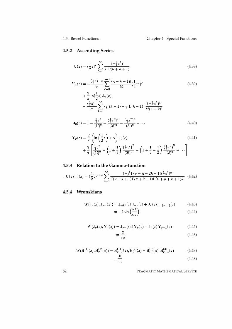
4.5. Bessel Functions Chapter 4. Special Functions
4.5.2 Ascending Series¿ ô ��Æ��{Iè� )/ Æ�� ô î�ï�� ? �°w "À Æ $ �òöé�=x� � rtò,r¶)³� (4.38)õ C ��Æ��{IÍw � "$ Æ�� ® �� C ® "�ï�� ? ���Vw¬òÕw�)³�<éòöé � )� Æ $ � ï (4.39)r /� �5 å� )/ Æ��U¿ C ��Æ��w � "$ Æ�� C� î�ï�� ? ��>G�qò6rL)´��r¬>G���åò6r¶)³�4� �°w "À Æ $ � ïòöé5����rtò7�<é¿ ? ��Æ��{IÍ)²w "À Æ $�°)!é^� $ r �´"À Æ $ � $� / é � $ w �´"À Æ $ � ê�q�7é^� $ r«ë�ë�ë (4.40)õ ?���Æ��{I /� ðæ�5 ©ð )/ Æ ñ r � ñ ¿!?���Æ�� (4.41)r /� � "À Æ $�°)!é^� $ w ð )xr )/ ñ u "À Æ $ w $� / é^� $ r ð )xr )/ r )�åñ u "À Æ $ w ê�q�7é^� $ w�ë�ë�ë �4.5.3 Relation to the Gamma-function¿ ô ��Æ��U¿ m �qÆ��{IN� )/ Æ�� ô � m î�ï�� ? �°w�� ï =}� � r r / òsr¶)³���³"À Æ $ � ï=}� � rtò~r¶)³�°=x� rnò6r¶)³�4=}� � r rnò6r¶)³��òöé (4.42)
4.5.4 Wronskians÷ �J¿ ô ��Æ���:�¿ ® ô ��Æ��4�{IÀ¿ ô � " �qÆ��(¿ ® ô ��Æ���ra¿ ô �qÆ��U¿ ® ô � "4¯ ��Æ�� (4.43)INw / '�3� .1 ���� Æ 2 (4.44)÷ �J¿ ô �qÆ��<: õ ô ��Æ��4�{IÀ¿ ô � " ��Æ�� õ ô ��Æ��2w¿ ô �qÆ�� õ ô � " �qÆ�� (4.45)I /� Æ (4.46)÷ �Jö "4¯ô ��Æ���:3ö $ ¯ô ��Æ��4�{IÀö "4¯ô � " �qÆ��<:3ö $ ¯ô �qÆ��Èwö "4¯ô ��Æ���:�ö $ ¯ô � " �qÆ�� (4.47)INw � �� Æ (4.48)
82 PRAGMATIC MATHEMATICAL SERVICE

Chapter 4. Special Functions 4.5. Bessel Functions
4.5.5 Asymptotic Expansions for Large Arguments
Principal Asymptotic Forms
For � fixed and Abà g¿ ô �qÆ��{I \ /� Æ ð %<&�' ð Æ,w )/ ��� w )� � ñ rv0 e � D e � 1 à Æöà ® " 2 ñ for à �,W3^{Æöà! �(4.49)õ ô|�qÆ��{I \ /� Æ ð7'435 ©ð7Æ6w )/ ��� w )� � ñ rn0 e � D e � 1�à Æöà ® " 2 ñ for à �jW�^}Æ�à� �(4.50)ö "°¯ô �qÆ�� 7 \ /� Æ 0 � D�® ä÷ ô ª ® ä� ª�¯ for w � ��jW�^}Æ� / � (4.51)ö $ ¯ô �qÆ�� 7 \ /� Æ 0 � D�® ä÷ ô ª ® ä� ª�¯ for w / � ��,W3^{Æ � (4.52)
Hankel’s Expansion
With AOILÆ6w � �´"$ � r "À �¿9ô|�qÆ��{I \ /� Æ �åk�� � :�Æ��|%�&('�AµwaøË� � :�Æ��|'�3� ±A�� for à �,W3^{Æöà� � (4.53)õ ô �qÆ��{I \ /� Æ �JkÁ� � :�Æ��7'435 ±AµwsøÇ� � :�Æ��|%�&('|Aö� for à �,W3^}Æöà� � (4.54)ö "°¯ô �qÆ��@I \ /� Æ �åk�� � :�Æ���rv�UøÇ� � :�Æ��4�70 �5Ò for w � ��jW�^}Æ� / � (4.55)
ö $ ¯ô �qÆ��{I \ /� Æ �Jk�� � :�Æ��Èwe�UøÇ� � :�Æ��4�|0 ®ö��Ò for w / � ��,W3^{Æ) � (4.56)
With I � � $k�� � :�Æ��{I î�ï�� ? �°w6)´� ï � : / ò� / Æ�� $ ï (4.57)Iè)²w � w�)³��� we���/ é ��õ(Æ�� $ r � wt)´�<� wy�(��� w / ó!��� w � �(�� é ��õ(Æ�� À wtë�ë�ë (4.58)
PRAGMATIC MATHEMATICAL SERVICE 83
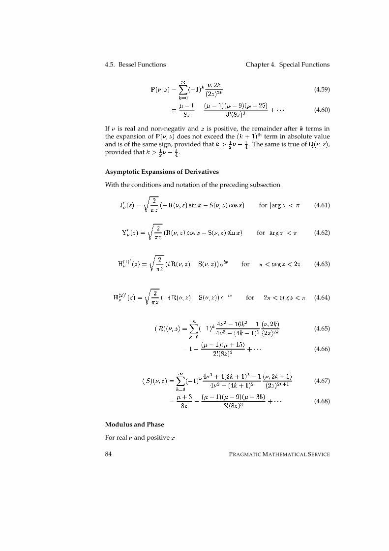
4.5. Bessel Functions Chapter 4. Special FunctionskÁ� � :�Æ��@Ilî�ï�� ? �°w6)´� ï � : / ò� / Æ�� $ ï (4.59)I w�)õ!Æ w � wt)´�<� wy�(��� w / ó!��7é ��õ(Æ�� ê r¶ë�ë�ë (4.60)
If � is real and non-negativ and Æ is positive, the remainder after ò terms inthe expansion of k�� � :�Æ�� does not exceed the �zò�rè)´� th term in absolute valueand is of the same sign, provided that ò ( "$ � w "À . The same is true of øË� � :�Æ�� ,provided that ò (�"$ � w êÀ .
Asymptotic Expansions of Derivatives
With the conditions and notation of the preceding subsection¿ â ô �qÆ��{I \ /� Æ �4wúù6� � :�Æ��|'�3� ±Aµw`~*� � :�Æ��|%�&('�A�� for à �,W3^}Æöà� � (4.61)õ â ô �qÆ��{I \ /� Æ �åùÕ� � :�Æ��7%<&('�A#w4~*� � :�Æ��|'�35 SAö� for à �jW�^{Æ�à! � (4.62)
ö "4¯ �ô ��Æ��{I \ /� Æ ���9ù~� � :�Æ��Èw`~*� � :�Æ��4��0 ��Ò for w � ��,W3^xÆ� / � (4.63)
ö $ ¯ �ô ��Æ��{I \ /� Æ �4w²�Sù6� � :�Æ��Èw`~*� � :�Æ��4�|0 ®ö��Ò for w / � ��,W3^{Æ) � (4.64)
� { ��� � :�Æ��{I î�ï�� ? �°w6)´� ï � � $ r¶) ì ò $ wt)� � $ wÔ� � òÇw�)³� $ � � : / ò7�� / Æ�� $ ï (4.65)Iè)²w � wt)´�<� r¶)³ó(�/ é5�qõ!Æ�� $ rLë�ë�ë (4.66)
�(1{�<� � :�Æ��@Ilî�ï�� ? �°w6)³� ï � � $ r � � / ò,r¶)³� $ wt)� � $ wÔ� � ò6r¶)³� $ � � : / ò6rL)´�� / Æ�� $ ï � " (4.67)I rn�õ(Æ w � w�)³��� we���<� rn�(ó(��7é ��õ!Æ�� ê rLë�ë�ë (4.68)
Modulus and Phase
For real � and positive A84 PRAGMATIC MATHEMATICAL SERVICE

Chapter 4. Special Functions 4.6. Beta Functions
4.6 Beta Functions
4.6.1 Beta function ûiù7üLýfþ(ûThe Beta function, also known as the Euler integral of the first kind, is definedby the integral8s��9�:�;<�xI \ "? A ¡³® " �4)²wGAö� 9 ® " a A for k´9:_; l �O[
� Q k´� l (4.69)
The Beta function can be extended to the complex plane by analytic continu-ation. One of the possible results is also the identity used in the implementa-tion5. 8,��9�:_;<�{I =�9�=}�q;��=x��9,rn;<� for k³9�:�;�:�9Árt; l �i\yQ k´�7:�Y
®l (4.70)
From the identity above it is obvious that the function is symmetric8Á�q9:_;<�{I«8s�z;´:�9|� (4.71)
Some interesting identities: ð � ò�ñ I )���µr¶)³�|8,���Ow¬ò,r«)(:�ò,rL)´� (4.72)
8,��9�:�;��|8,��9sr�;´:�)±wy;<�{I �A�'�3� �� � A�� (4.73)
4.6.2 Incomplete Beta Function
The incomplete beta function is the generalization of the beta function and is,like the incomplete gamma function, defined by the indefinite integral8Á��Ahw�9:_;<�}I \ Ò? � ¡´® " �4)²wG�4� 9 ® " a � (4.74)
From which follows 8s�4),w�9:_;<�{IL8,�q9:_;<� (4.75)
The incomplete beta function is related to the hypergeometric function8,��A�w�9�:�;<�{I«9 ® " A ¡Ãÿ ��9�:�)²w¬;fw�9,rL)Æw4Aö� (4.76)
The implementation of the incomplete beta function is by means of the regu-larized beta function.
5With the exception that the current implementation of the Gamma-function is for �����;¥���� Õonly.
PRAGMATIC MATHEMATICAL SERVICE 85

4.7. Gamma Functions Chapter 4. Special Functions
4.6.3 Regularized Incomplete Beta Function
The regularized incomplete beta function� Ò ��9�:�;��{I 8s��A�w�9�:�;<�� �q9:_;<� (4.77)
It is implemented with the continued fraction given at[122].� D ��9�:�;��{I Æ ¡ �°)²wyÆ�� 99S8Á�q9:_;<� ))xr * �4)³�)xr * � / �)xr * �����)xr * � � �)xr * �zó!�)xr¶ë�ë�ë(4.78)
* � / �#rL)´�{Ièw Æ�q9Árv�å�<��96rt;2rv�å��q9sr / �å�<�q9sr / �µrL)´�* � / �å�xI Æ(�{�q;}we�å��q9sr / �Owt)´�<��96r / �å�4.7 Gamma Functions
4.7.1 � -function
The = -function is the generalized factorial A�é .=x��ÆÁr¶)³�{I«Æé for Æ6w�) �VW � Q k³� l (4.79)
It is defined for all Æ �V\yQ k´�7:�Y ® l by the integral=}�qÆ��{I \ î? � D�® " 0 ® " a � (4.80)
The picture on the frontpage is a plot of the values of =}��A�� with A �i[ 1ew ì �A � ì . It is the result of the following Gnuplot-script �1 s e t terminal p o s t s c r i p t eps enhanced s o l i d ” Helvet i ca ”
142 s e t output ”gammafunction . eps”3 s e t zeroaxis4 s e t nokey5 s e t parametric6 s e t s ize r a t i o � 1 1 ,17 s e t trange [ � 6:6]8 s e t xrange [ � 6 : 6 ] ; s e t yrange [ � 6:6]9 s e t samples 15000
86 PRAGMATIC MATHEMATICAL SERVICE

Chapter 4. Special Functions 4.7. Gamma Functions
10 f ( x ) = ( � pi ) /(x � gamma( abs ( x ) ) � sin ( pi � x ) )11 plot t , ( t � 0)? f ( t ) :gamma( t ) �The =}���� -function is implemented here with the common Lanczos approxi-
mation6. =}��Æ��@I . / � �qÆÁr�íÁwe� � ó(� D�® ? = �0 D_� ô ® ? = � * � ? �C � " =>=>= < � CÆ�r¬� + (4.81)
The values of � ? ����� � <� ? � � �(�!�(�!�!�(�!�(�!�!�(�!õ��(���!�� " ì í ì � ó / �(� ì õ�) / )�õ!õ�ó|)� $ w6) / ó!� � )³�!� / ) ì í /(/ � � / õ� ê í!í|) � � / � � / õ�í!í(í ì ó!�7)��� À w6)´í ì � ì )³ó!� / ��) ì / ) � �(ó��� � ) /�� ó!��í�� � � / í�õ ì õ ì ����ó� � w�� � )³�!õ�ó(í�)³�!��ó / ì ó(í / �|) /� ô � � �(õ � � ì ��ó(í�õ!�7)³�(ó!í|) ì 0{w ì� < ) � ó!�(ó ì � / í���ó|) � �!�|)() ì 0{w¬íNegative non-integer values of Æ are computed by the way of the identity=}�4w�Æ��{I w �Æ(=x��Æ��|'435 � Æ (4.82)
The logarithm of the = -function is implemented as=x��Æ��{Iè�z9~wy� � ó!���5 ~��96rtíÁwy� � ó!�ÈwÔ��9,rtíÁwy� � ó!�r �� * . / � * � ? �C � " =>=>= < � CÆ�r¬�C+Q+ (4.83)
And the logarithm of the = -function of the negative non-integer values by=}�4w�Æ��{I �� Õ��à =x��Æ���à � (4.84)
Viktor T. Thot gave in [106] a simple way to produce arbitrary precisionvalues for =}��Æ�� with Æ)�O\ with the following formulas7�5 �=}�qÆÁrL)´�{I �5 � ��¶r«�qÆ�rn� � ó!�æ�� ~�qÆÁr ç rv� � ó(�Èw��qÆÁr ç rv� � ó(� (4.85)
With the row vector vI � ) )Æ�rL) )Æsr / ����� )Æsr¬�Owt) � (4.86)
6The algorithm has been implemented for rationals only at the time of this writing.7C++-code can be found at the webpage linked from [106]
PRAGMATIC MATHEMATICAL SERVICE 87

4.7. Gamma Functions Chapter 4. Special Functions� the product of the �yT¸� matrices �G:�K¸:¹. and the column vector �K ��� I ¹º» º¼
) if �2I«�w6) �<®ö� u �����<® "�<® " w if � (Ô�7: ½�¾ �� otherwise(4.87)
. ��� I ¹º» º¼"$ if �2I ½ I«�� if
½ (��w6) ��®7� F � ï�� ? u $ �$ ï w u ïï ���<®ö� w otherwise(4.88)
� ��� I ¹ººººº» ººººº¼� if � HI ½) if �@I ½ I«�w6) if �@I ½ IN)� ��® " ® �<® " / � / ��w�)³��åw�) otherwise
(4.89)
� � I � / �°�_é�0 ��� � � ? = ��_é / $ ��® " �q�ör ç rn� � ó!� �5� ? = � (4.90)
The typical error can be calculated with� IE.�� (4.91)
à à!I ������/ . / 0 * 0 � . � w C
® "� � � ? w6) � �z¨Õ� � + ����� (4.92)
Another way are the polynomial approximations for values ���nAá� ) withthe coefficients as listed in [1] p.257.=}��A2r¸)´�{IÍ)�rË9 " A@rË9 $ A $ rË9 ê Aê�rË9�À�A À rË9 � A � r ��Aö� à ��A���àæ�Ló@T6)³� ® � (4.93)9 " INw � ó�í � õ ì � ì 9(ÀÁI � � / � ó(ó � � (4.94)9 $ I � �(ó7) / � ì � 9 � Ièw � )³�7)�� ì í�õ9 ê INw � ì �!�(õ(ó@õ(õAnd with a slightly smaller error=}��AËr¶)³�{IÍ)xrt; " AËrn; $ A $ rLë�ë�ë³rt; < A < r ��A�� à ��A���à,����Te)�� ® ô (4.95); " IÍw � ó(í!í|)��²) ì ó / ; � INw � í�ó ì í�� � ��í�õ (4.96); $ I � �(õ!õ / �}ó�õ(�7) ; � I � � õ / )��{�(�!� �; ê IÍw � õ!��í��(ó ì �!��í ; ô INw � )��!��ó / í�õ7)³õ;�ÀÁI � ��)�õ / � ì õ�ó(í ; < I � �!�(ó!õ ì õ(� � �88 PRAGMATIC MATHEMATICAL SERVICE
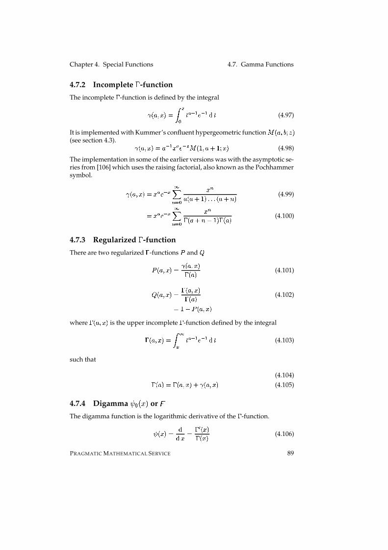
Chapter 4. Special Functions 4.7. Gamma Functions
4.7.2 Incomplete � -function
The incomplete = -function is defined by the integral� �q9�:4A��xI \ Ò? � ¡³® " 0 ® " a � (4.97)
It is implemented with Kummer’s confluent hypergeometric function� ��9�:_;fw�Æ��
(see section 4.3). � ��9�:4Aö�{I¶9 ® " A ¡ 0 ®AD � �4)!:�9,rL)Æw4Aö� (4.98)
The implementation in some of the earlier versions was with the asymptotic se-ries from [106] which uses the raising factorial, also known as the Pochhammersymbol. � ��9�:4Aö�{ILA ¡ 0 ®�Ò î�C � ? A C9ö��9,rL)´� ����� ��9,r¬�å� (4.99)ILA ¡ 0 ®�Ò î�C � ? A C=}�q9srv�#rL)´�°=}�q9|� (4.100)
4.7.3 Regularized � -function
There are two regularized = -functions � and �����9�:4Aö�{I � ��9�:�A��=x��9|� (4.101)����9�:4Aö�{I =x��9�:4Aö�=}�q9�� (4.102)Iè)²w4����9�:�A��where =}�q9:�A�� is the upper incomplete = -function defined by the integral=x��9�:4Aö�{I \ îÒ � ¡³® " 0 ® " a � (4.103)
such that
(4.104)=x��9|�{I¶=x��9�:4Aö�år � �q9:�A�� (4.105)
4.7.4 Digamma � ¥ ù��xû or �The digamma function is the logarithmic derivative of the = -function.>Á��A��}I aa A I = â ��A��=}��A�� (4.106)
PRAGMATIC MATHEMATICAL SERVICE 89
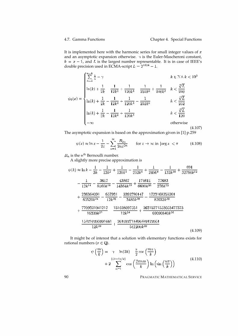
4.7. Gamma Functions Chapter 4. Special Functions
It is implemented here with the harmonic series for small integer values of Aand an asymptotic expansion otherwise. � is the Euler-Mascheroni constant,òtI AGw ) , and · is the largest number representable. It is in case of IEEE’sdouble precision used in ECMA-script ·nI / " ? $ À w�) .> ? ��A��}I
¹ºººººººººººººººº» ºººººººººººººººº¼
C �åïFC � " "C w � ò �VW�1iò «)³� ê�� È�qò7�år )/ ò w )) / ò $ r )) / �(ò À w )/ ó / ò � r )/ � �(ò < ò y. ·/ � ��� È�qò7�år )/ ò w )) / ò $ r )) / �(ò À w )/ ó / ò � ò �. ·/ ó /�� È�qò7�år )/ ò w )) / ò $ r )) / �(ò À ò �. ·) / �règ otherwise(4.107)
The asymptotic expansion is based on the approximation given in [1] p.259>s��Æ�� 7 �5 �Æ6w )/ Æ w î�C � "� $ C/ ��Æ $ C for Æ àâg in à �jW�^{Æöà! � (4.108)� C is the � th Bernoulli number.
A slightly more precise approximation is>s�qò7� 7 �5 �òËw )/ ò w )) / ò $ r )) / ��ò À w )/ ó / ò � r )/ � �(ò < w ))�� / ò " ? r ì �7)� / í ì �(ò " $w )) / ò " À r � ì )´íõ�) ì �(ò " � w � �!õ ì í) � � ì � ò " < r )�í � ì )!)ì!ì �!��ò $ ? w í(í ì õ(�/ í ì ò $�$r / � ì � ì � �!�7)ì ó!ó / �(ò $ À w ì ó(í��(�7)) / ò $ � r �(�!� / í�õ(�7) � í� � õ(�(ò $ < w )´í / �7) ì õ / ó!ó / �7)õ�ó��!� / ò ê ?r í(í��!�(� / )�� � ) / )´í) ì � / ��ò ê $ w )´ó|) ì / õ ì ��í�ó!ó7)) / ò ê À r / ì ��)³ó / í�)´ó!ó��(�(ó�� � í!í���í´�ì �!�(�!�(õ � ��ò ê �w )´ó � / )�� / �(ó!�!��) ì!ì )) / ò ê < r / ì )��(õ / í|)�õ � � ì �!� ��) /!/ �(ó�)ó � ) / �(�(ò À ?(4.109)
It might be of interest that a solution with elementary functions exists forrational numbers ( A �VZ ).> 1 % ò 2iIèw � wN�� È� / ò7�Èw � / %�&��%1 % �ò 2r /�� ï ® "4¯J6 $���C � " %�&('�ð / � ��%ò ñ �� 1�'�3� 1 � �ò 2A2 (4.110)
90 PRAGMATIC MATHEMATICAL SERVICE
Chapter 4. Special Functions 4.7. Gamma Functions
All numbers in a computer are �ÍZ , so the above formula seems to be a fit-ting algorithm but the solution for some A is not in Z anymore, so any directimplementation would suffer from lost of precision.
4.7.5 Polygamma ���@ù��xûThe polygamma function >{C���Aö� is the � th derivative of the digamma function> ? ��A�� . > C ��Aö�}I a C >2?���Æ��a A (4.111)
It is implemented here, for positive integer orders only, with Hurwitz’ � -function.> C ��A��}I _ >2?(��A�� �©I«��4w6)³� C � " =x���µrL)´�4�7���#rL)(:4A��Ï�N�VW � (4.112)
4.7.6 Double Factorial
The double factorial A�é�é is implemented here as follows
Aåé5é�I ¹ººº» ººº¼undefined & a,a ���å�8�VY ®) �iIèw6)(:4�VI«�ã�äæå u �5 �=}� C � "$ rn� � ó!��r "8 :�$ C � "$ wG�5 å� . � � w & a,a �qY4à �}à [��8�OY ®ã�äæå u "8 :ö$ C $ r �� �= u C $ r¶) w w otherwise
(4.113)
4.7.7 Hyperfactorial
The logarithm of the hyperfactorial Dn���å� is implemented as
Dv���å�{I ¹º» º¼not defined here � H�OW �) �iI¶�F C� � " ���5 å���°� (4.114)
4.7.8 Raising Factorial (Pochhammer Symbol)
The raising factorial or Pochhammer symbol � C �q9�� is implemented in threedifferent ways:
By Product �ÈC*��9|�}I C�� � ? �q9,rv�°� (4.115)
PRAGMATIC MATHEMATICAL SERVICE 91

4.8. Error Function Chapter 4. Special Functions
By the = -Function � C ��9|�{I =}�q9,rv�å�=}�q9|� (4.116)
By the �5 �= -Function �5 X� C ��9|�{IN��� �=x��96r¬�å���2wÔ�V�5 �=}��9|��� (4.117)
4.7.9 K-Function
The definition of the K-function used here is �n���å��I Dv���©wL)³� where Dv���å� isthe hyperfactorial and �N�OW � .�t���å�{I¶� ? ) " / $ � ê ë�ë�ë³���Owt)´� C ® " (4.118)
The hyperfactorial function of the implementation returns the logarithm of thehyperfactorial and so does the implementation of the K-function in the imple-mentation.
4.7.10 Barne’s G-Function
Barne’s G-Function is defined as0 ���å�}I � =}���å�}� C ® "�n���å� _ ) if �©IL��7é5)!é / é�ë�ë�ë<���Ow / �<é if �N(t� (4.119)
Where the square brackets denote the rounding to the nearest integer.It is implemented with logarithmic calculations�5 0 ���å�{I ¹º» º¼
not defined � H�iW#��@) �©I¶��:4�VIN)!:��VI /�����Vw�)³�!�5 ²=}���å���2wN�� �t���å� (4.120)
with �n���å� the K-function at the positive integer � .
4.8 Error Function
The error function is defined by the integral 8ã»W3V�ÆÕI /. � \ D? 0 ® ÷ a � (4.121)
8From [1] p. 297 ff.
92 PRAGMATIC MATHEMATICAL SERVICE

Chapter 4. Special Functions 4.8. Error Function
The complemetary error functionã»W3V�%�ÆÕI /. � \ îD 0 ® ÷ a � (4.122)IN)²wGããW7V�Æwith the restriction that �jW�^v� à � with à � à� ª À as � à g and � I ª À if Ê8� $ isbounded to the left.
Another useful integralá ��Æ��{I¶0 ®�D ÷ ð*)xr / �. � \ D? 0 ÷ a � ñ (4.123)I¶0 ®�D ÷ ããW7V�%(�°w�Æ(�Ð�Several series expansions are possibleããW7V�ÆËI /. � î�C � ? �4w6)³� C Æ $ C
� "�@é � / ��r¶)³� (4.124)I /. � 0 ®�D ÷ î�C � ? / C)²ë��²ë�ë�ë�� / �µrL)´� Æ $ C � " (4.125)á �qÆ��xI î�C � ? �qÆ!�°� C= u C $ r¶) w (4.126)
Some useful symmetriesã»W3V��4w�Æ��@INwbããW7V�Æ (4.127)ã»W3V ÆÕI ã»W3V�Æ (4.128)á �°w�Æ��{I / 0 ®�D ÷ w á ��Æ�� (4.129)á � Æ��{I á �°w�Æ�� (4.130)
Continued fractions/ 0 D ÷ \ îD 0 ® ÷ a �{I )ÆÁr "$Æ�r )ÆÁr ê$Æsr /Æ�r¶ë�ë�ëfor 汮 (�� (4.131)
). � \ î® î 0® ÷ a �Æ~wG� I )Æ,w "$Æ6w )Æ6w ê$Æ,w /Æ~wtë�ë�ë
for ÌSÆ HIL� (4.132)
PRAGMATIC MATHEMATICAL SERVICE 93

4.9. Generalized Laguerre Function Chapter 4. Special Functions
With A C ¯ï the zeros and D C ¯ï the weight factors of the Hermite polynomials theformula in 4.132 can be described as). � �53#�C$� î C�ï�� " D C ¯ïÆ6weA C ¯ï (4.133)
The error function is related to the confluent hypergeometric function (seesection 4.3) ã»W3V�ÆÇI / Æ. �"! ð )/ : � / :�w�Æ $ ñ (4.134)I / Æ. � 0 ®�D ÷ ! ð )(: � / :�w�Æ $ ñWhich leads to the implementations for Aá�V[ã»W3V7AOIL'�3Ô^( å��Aö� � u "$ :4A $ w. � (4.135)ã»W3V�%�ÆÕIÍ)²wNã»W3V�A (4.136)
Two other approximations for Aá�VZ �?ã»W3V7AOIN)²w )�4)xrv9 " A�rv9 $ A $ rn9 ê A ê rn9�À�A À � À r ��A�� with à ��A���àæ�LóËTG)³� ® À(4.137)9 " I �^/ í�õ!�(�{� 9 $ I �^/ �(�!�!õ}� (4.138)9 ê I � �!�(�!��í / 9 À I � ��í�õ7)��}õã»W3V7A¸Iè)²w )�°)xrn9 " AËrn9 $ A $ r¶ë�ë�ë´rv9 � A � � � r ��A�� with à ��A���à!�Ô��TG)³� ® ô(4.139)9 " I � ��í���ó / �(��í�õ � 9 $ I � � � /(/ õ / �7) / � (4.140)9 ê I � �!�!� / í2��ó / í � 9(ÀÁI � �!�!��)³ó / �7) � �9 � I � �!�!� / í ì ó ì í / 9 � I � �!�!�(� � �(� ì �!õ
4.9 Generalized Laguerre Function
4.10 # (Riemann, Hurwitz), $ %�4.10.1 Riemann’s ø -Function
For the right halfplane by means of the Dirchlet % -function�7� '³�{I ))²w / " ® @ î�C � ? �°w6)³� C® "� @ (4.141)
94 PRAGMATIC MATHEMATICAL SERVICE

Chapter 4. Special Functions 4.10. � (Riemann, Hurwitz), DGECFor the entire complex plane without 'sIè) ([43])��� '´�}I ))²w / " ® @ î�C � ? )/ C � " C�ï�� ? �°w6)´� ï ð � ò�ñ �qò6r¶)³� ® @ (4.142)
For even �N�OW and � ¾ / �7���å�}I / C ® " à � C à � C���å��é (4.143)
and for odd �N�OW and � ¾ ) �7�°w²�å�{INw � C � "�µrL) (4.144)
where
� C are Bernoulli numbers.
Derivatives
The derivative of the Riemann � -function is defined for the right half-plane by� â � '´�{INw î�C'&)(+* " ® $-, �� ²�� @ (4.145)
For/ �N�VW and � ¾ )� â �4w / �å�@I �°w6)³� C �7� / �µrL)´�<� / �å��é/ $ C � " � $ C (4.146)
4.10.2 Hurwitz’ ø -Function
4.10.3 General Partial Harmonic Function .0/�The general partial harmonic function D EC is implemented with the summationformula D EC I C� � � " )� E (4.147)
4.10.4 Partial Harmonic Function . ß�The partial harmonic function D "C is implemented in two ways: with simplesummation up to �iIN)å�!�(� and an asymptotic series approximation otherwise.
D�C�I ¹» ¼F C�5� " " � with �G )å�!�(�� r �� å���å�år )/ � w )) / � $ r )) / �!� À with � ¾ )å�!�(� (4.148)
PRAGMATIC MATHEMATICAL SERVICE 95

4.10. � (Riemann, Hurwitz), DGEC Chapter 4. Special Functions
That limit is not as arbitrary as it seems to be. With æ ���å� the summation func-tion in ECMA-script, ç ���å� a high precision calculation9 and D����å� the asymptoticapproximation as described above.æ ���å�{I«í � � õ(ó � í��{õ ì �}ó(ó��@� ��� ) ì � /ç ���å�{I«í � � õ(ó � í��{õ ì �}ó(ó��@� � � / í!ó2�Då���å�}I«í � � õ(ó � í��{õ ì �}ó(ó��@� ��� �|) / ì ó ì ó7)�õ / � � �!��� ����� � º�º� �©Iè)å�(�!� (4.149)
æ ���å�{IÍ) /|� �!�(�²) � ì ) / �{õ ì � � / �±)³õ|)ç ���å�{IÍ) /|� �!�(�²) � ì ) / �{õ ì � / õ7)�í � �Då���å�}IÍ) /|� �!�(�²) � ì ) / �{õ ì � � / íÈ� � í2� ì � / )��@� ì �}ó�� � ����� � º�º� �iIè)³�!�{�(�!� (4.150)
14 decimal digits of precision for �G�VW seem sufficient.
9With GNU’s bc(1) with the summation formula and scale=100
96 PRAGMATIC MATHEMATICAL SERVICE
Chapter 5
Linear Algebra (Matrices)
5.1 Matrix Decompositions
5.1.1 Eigen Decomposition
5.1.2 LU Decomposition
5.1.3 QR Decomposition
5.1.4 Singular Value Decomposition
5.2 Systems of Equations
5.2.1 Determinant
97

Chapter 6
Sets
The set arithmetic used here is based on the common Zermel-Fraenklin axioms.If H©:�K are subsets of a universe 1 than the basic operations are the equality,union, intersection, difference, power, and the Cartesian product.
Sets are implemented in this program as simple arrays.
6.1 Equality 2 354Two sets H©:�K are equal if both sets have the same elements.� H©:�K¸:4AÈ��A �iH � � Aá�VK��}I � ��H I¶K�� (6.1)
6.2 Union 2 674
898989898989898989898989889898989898989898989898988989898989898989898989898898989898989898989898989889898989898989898989898988989898989898989898989898898989898989898989898989889898989898989898989898988989898989898989898989898898989898989898989898989889898989898989898989898988989898989898989898989898:9:9:9:9:9:9:9:9:9:9:9:9::9:9:9:9:9:9:9:9:9:9:9:9::9:9:9:9:9:9:9:9:9:9:9:9::9:9:9:9:9:9:9:9:9:9:9:9::9:9:9:9:9:9:9:9:9:9:9:9::9:9:9:9:9:9:9:9:9:9:9:9::9:9:9:9:9:9:9:9:9:9:9:9::9:9:9:9:9:9:9:9:9:9:9:9::9:9:9:9:9:9:9:9:9:9:9:9::9:9:9:9:9:9:9:9:9:9:9:9::9:9:9:9:9:9:9:9:9:9:9:9::9:9:9:9:9:9:9:9:9:9:9:9:
;9;9;9;9;9;9;9;9;9;9;9;9;9;;9;9;9;9;9;9;9;9;9;9;9;9;9;;9;9;9;9;9;9;9;9;9;9;9;9;9;;9;9;9;9;9;9;9;9;9;9;9;9;9;;9;9;9;9;9;9;9;9;9;9;9;9;9;;9;9;9;9;9;9;9;9;9;9;9;9;9;;9;9;9;9;9;9;9;9;9;9;9;9;9;;9;9;9;9;9;9;9;9;9;9;9;9;9;;9;9;9;9;9;9;9;9;9;9;9;9;9;;9;9;9;9;9;9;9;9;9;9;9;9;9;;9;9;9;9;9;9;9;9;9;9;9;9;9;;9;9;9;9;9;9;9;9;9;9;9;9;9;;9;9;9;9;9;9;9;9;9;9;9;9;9;;9;9;9;9;9;9;9;9;9;9;9;9;9;<9<9<9<9<9<9<9<9<9<9<9<9<9<<9<9<9<9<9<9<9<9<9<9<9<9<9<<9<9<9<9<9<9<9<9<9<9<9<9<9<<9<9<9<9<9<9<9<9<9<9<9<9<9<<9<9<9<9<9<9<9<9<9<9<9<9<9<<9<9<9<9<9<9<9<9<9<9<9<9<9<<9<9<9<9<9<9<9<9<9<9<9<9<9<<9<9<9<9<9<9<9<9<9<9<9<9<9<<9<9<9<9<9<9<9<9<9<9<9<9<9<<9<9<9<9<9<9<9<9<9<9<9<9<9<<9<9<9<9<9<9<9<9<9<9<9<9<9<<9<9<9<9<9<9<9<9<9<9<9<9<9<<9<9<9<9<9<9<9<9<9<9<9<9<9<<9<9<9<9<9<9<9<9<9<9<9<9<9<
A B
U
Figure 6.1: H MOKThe union of the two sets HF:�K is defined asHRM¸K I�k�A2à A��OH>=ÇAá�VK l (6.2)
The implementation of the union concatenates both arrays, sorts the result andremoves all non-unique entries. That is admittedly not the fastest way to do it.
98
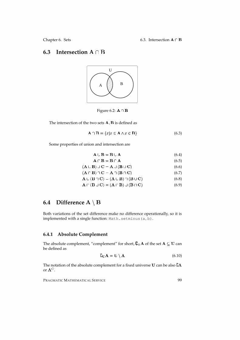
Chapter 6. Sets 6.3. Intersection H POK6.3 Intersection 2 ?74
A B
U
Figure 6.2: HNP¸KThe intersection of the two sets H©:�K is defined asH P¸KRI k³AÈà Aá�VHÀ1ÇAá�OK l (6.3)
Some properties of union and intersection areHNM¸K I¶K«MOH (6.4)HNP¸K I¶K«POH (6.5)�qH MOKË�*Mú.RI¶HNMe��K Mú.Ç� (6.6)�qH POKË�*Pú.RI¶HNPe��K Pú.Ç� (6.7)HRMF�zK«Pú.Ë�{IN�qH M#K���Pe��K M .Ë� (6.8)HRPF�zK«Mú.Ë�{IN�qH P#K���Me��K P .Ë� (6.9)
6.4 Difference 2 @A4Both variations of the set difference make no difference operationally, so it isimplemented with a single function: Math.setminus(a,b).
6.4.1 Absolute Complement
The absolute complement, “complement” for short, B9C�H of the set H /D1 canbe defined as B C HÓI>1RQSH (6.10)
The notation of the absolute complement for a fixed universe 1 can be also B�Hor HFE .
PRAGMATIC MATHEMATICAL SERVICE 99
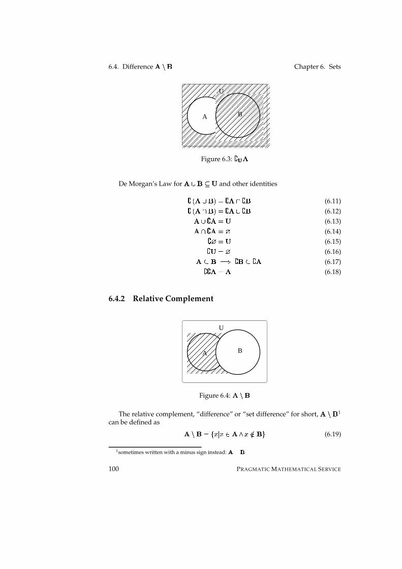
6.4. Difference H QSK Chapter 6. Sets
G9G9G9G9G9G9G9G9G9G9G9G9G9G9G9G9G9G9G9G9G9G9G9G9G9GG9G9G9G9G9G9G9G9G9G9G9G9G9G9G9G9G9G9G9G9G9G9G9G9G9GG9G9G9G9G9G9G9G9G9G9G9G9G9G9G9G9G9G9G9G9G9G9G9G9G9GG9G9G9G9G9G9G9G9G9G9G9G9G9G9G9G9G9G9G9G9G9G9G9G9G9GG9G9G9G9G9G9G9G9G9G9G9G9G9G9G9G9G9G9G9G9G9G9G9G9G9GG9G9G9G9G9G9G9G9G9G9G9G9G9G9G9G9G9G9G9G9G9G9G9G9G9GG9G9G9G9G9G9G9G9G9G9G9G9G9G9G9G9G9G9G9G9G9G9G9G9G9GG9G9G9G9G9G9G9G9G9G9G9G9G9G9G9G9G9G9G9G9G9G9G9G9G9GG9G9G9G9G9G9G9G9G9G9G9G9G9G9G9G9G9G9G9G9G9G9G9G9G9GG9G9G9G9G9G9G9G9G9G9G9G9G9G9G9G9G9G9G9G9G9G9G9G9G9GG9G9G9G9G9G9G9G9G9G9G9G9G9G9G9G9G9G9G9G9G9G9G9G9G9GG9G9G9G9G9G9G9G9G9G9G9G9G9G9G9G9G9G9G9G9G9G9G9G9G9GG9G9G9G9G9G9G9G9G9G9G9G9G9G9G9G9G9G9G9G9G9G9G9G9G9GG9G9G9G9G9G9G9G9G9G9G9G9G9G9G9G9G9G9G9G9G9G9G9G9G9GG9G9G9G9G9G9G9G9G9G9G9G9G9G9G9G9G9G9G9G9G9G9G9G9G9GG9G9G9G9G9G9G9G9G9G9G9G9G9G9G9G9G9G9G9G9G9G9G9G9G9GG9G9G9G9G9G9G9G9G9G9G9G9G9G9G9G9G9G9G9G9G9G9G9G9G9GG9G9G9G9G9G9G9G9G9G9G9G9G9G9G9G9G9G9G9G9G9G9G9G9G9GG9G9G9G9G9G9G9G9G9G9G9G9G9G9G9G9G9G9G9G9G9G9G9G9G9GH9H9H9H9H9H9H9H9H9H9H9H9H9H9H9H9H9H9H9H9H9H9H9H9H9HH9H9H9H9H9H9H9H9H9H9H9H9H9H9H9H9H9H9H9H9H9H9H9H9H9HH9H9H9H9H9H9H9H9H9H9H9H9H9H9H9H9H9H9H9H9H9H9H9H9H9HH9H9H9H9H9H9H9H9H9H9H9H9H9H9H9H9H9H9H9H9H9H9H9H9H9HH9H9H9H9H9H9H9H9H9H9H9H9H9H9H9H9H9H9H9H9H9H9H9H9H9HH9H9H9H9H9H9H9H9H9H9H9H9H9H9H9H9H9H9H9H9H9H9H9H9H9HH9H9H9H9H9H9H9H9H9H9H9H9H9H9H9H9H9H9H9H9H9H9H9H9H9HH9H9H9H9H9H9H9H9H9H9H9H9H9H9H9H9H9H9H9H9H9H9H9H9H9HH9H9H9H9H9H9H9H9H9H9H9H9H9H9H9H9H9H9H9H9H9H9H9H9H9HH9H9H9H9H9H9H9H9H9H9H9H9H9H9H9H9H9H9H9H9H9H9H9H9H9HH9H9H9H9H9H9H9H9H9H9H9H9H9H9H9H9H9H9H9H9H9H9H9H9H9HH9H9H9H9H9H9H9H9H9H9H9H9H9H9H9H9H9H9H9H9H9H9H9H9H9HH9H9H9H9H9H9H9H9H9H9H9H9H9H9H9H9H9H9H9H9H9H9H9H9H9HH9H9H9H9H9H9H9H9H9H9H9H9H9H9H9H9H9H9H9H9H9H9H9H9H9HH9H9H9H9H9H9H9H9H9H9H9H9H9H9H9H9H9H9H9H9H9H9H9H9H9HH9H9H9H9H9H9H9H9H9H9H9H9H9H9H9H9H9H9H9H9H9H9H9H9H9HH9H9H9H9H9H9H9H9H9H9H9H9H9H9H9H9H9H9H9H9H9H9H9H9H9HH9H9H9H9H9H9H9H9H9H9H9H9H9H9H9H9H9H9H9H9H9H9H9H9H9HH9H9H9H9H9H9H9H9H9H9H9H9H9H9H9H9H9H9H9H9H9H9H9H9H9H
U
I9I9I9I9I9I9I9I9I9I9I9I9I9II9I9I9I9I9I9I9I9I9I9I9I9I9II9I9I9I9I9I9I9I9I9I9I9I9I9II9I9I9I9I9I9I9I9I9I9I9I9I9II9I9I9I9I9I9I9I9I9I9I9I9I9II9I9I9I9I9I9I9I9I9I9I9I9I9II9I9I9I9I9I9I9I9I9I9I9I9I9II9I9I9I9I9I9I9I9I9I9I9I9I9II9I9I9I9I9I9I9I9I9I9I9I9I9II9I9I9I9I9I9I9I9I9I9I9I9I9II9I9I9I9I9I9I9I9I9I9I9I9I9II9I9I9I9I9I9I9I9I9I9I9I9I9II9I9I9I9I9I9I9I9I9I9I9I9I9II9I9I9I9I9I9I9I9I9I9I9I9I9IJ9J9J9J9J9J9J9J9J9J9J9J9J9JJ9J9J9J9J9J9J9J9J9J9J9J9J9JJ9J9J9J9J9J9J9J9J9J9J9J9J9JJ9J9J9J9J9J9J9J9J9J9J9J9J9JJ9J9J9J9J9J9J9J9J9J9J9J9J9JJ9J9J9J9J9J9J9J9J9J9J9J9J9JJ9J9J9J9J9J9J9J9J9J9J9J9J9JJ9J9J9J9J9J9J9J9J9J9J9J9J9JJ9J9J9J9J9J9J9J9J9J9J9J9J9JJ9J9J9J9J9J9J9J9J9J9J9J9J9JJ9J9J9J9J9J9J9J9J9J9J9J9J9JJ9J9J9J9J9J9J9J9J9J9J9J9J9JJ9J9J9J9J9J9J9J9J9J9J9J9J9JJ9J9J9J9J9J9J9J9J9J9J9J9J9J
A B
Figure 6.3: B C HDe Morgan’s Law for H MOK`/A1 and other identitiesB±�qHNM¸K��{IKB�HNPLB�K (6.11)B±�qHNP¸K��{IKB�HNMLB�K (6.12)H MLB�H�I>1 (6.13)H PLB�H�IKM (6.14)BNM«I>1 (6.15)B'1JIKM (6.16)H /�K I � B�K`/OB�H (6.17)BNB�H�I«H (6.18)
6.4.2 Relative Complement
U
P9P9P9P9P9P9P9P9P9P9P9PP9P9P9P9P9P9P9P9P9P9P9PP9P9P9P9P9P9P9P9P9P9P9PP9P9P9P9P9P9P9P9P9P9P9PP9P9P9P9P9P9P9P9P9P9P9PP9P9P9P9P9P9P9P9P9P9P9PP9P9P9P9P9P9P9P9P9P9P9PP9P9P9P9P9P9P9P9P9P9P9PP9P9P9P9P9P9P9P9P9P9P9PP9P9P9P9P9P9P9P9P9P9P9PP9P9P9P9P9P9P9P9P9P9P9PP9P9P9P9P9P9P9P9P9P9P9PQ9Q9Q9Q9Q9Q9Q9Q9Q9Q9Q9QQ9Q9Q9Q9Q9Q9Q9Q9Q9Q9Q9QQ9Q9Q9Q9Q9Q9Q9Q9Q9Q9Q9QQ9Q9Q9Q9Q9Q9Q9Q9Q9Q9Q9QQ9Q9Q9Q9Q9Q9Q9Q9Q9Q9Q9QQ9Q9Q9Q9Q9Q9Q9Q9Q9Q9Q9QQ9Q9Q9Q9Q9Q9Q9Q9Q9Q9Q9QQ9Q9Q9Q9Q9Q9Q9Q9Q9Q9Q9QQ9Q9Q9Q9Q9Q9Q9Q9Q9Q9Q9QQ9Q9Q9Q9Q9Q9Q9Q9Q9Q9Q9QQ9Q9Q9Q9Q9Q9Q9Q9Q9Q9Q9QQ9Q9Q9Q9Q9Q9Q9Q9Q9Q9Q9Q
A B
Figure 6.4: HRQSKThe relative complement, “difference” or “set difference” for short, H Q²K 1
can be defined as HRQSKRI k�AÈà Aá�VHÀ1ËAÁ}�VK l (6.19)
1sometimes written with a minus sign instead: R¬Ý�S100 PRAGMATIC MATHEMATICAL SERVICE
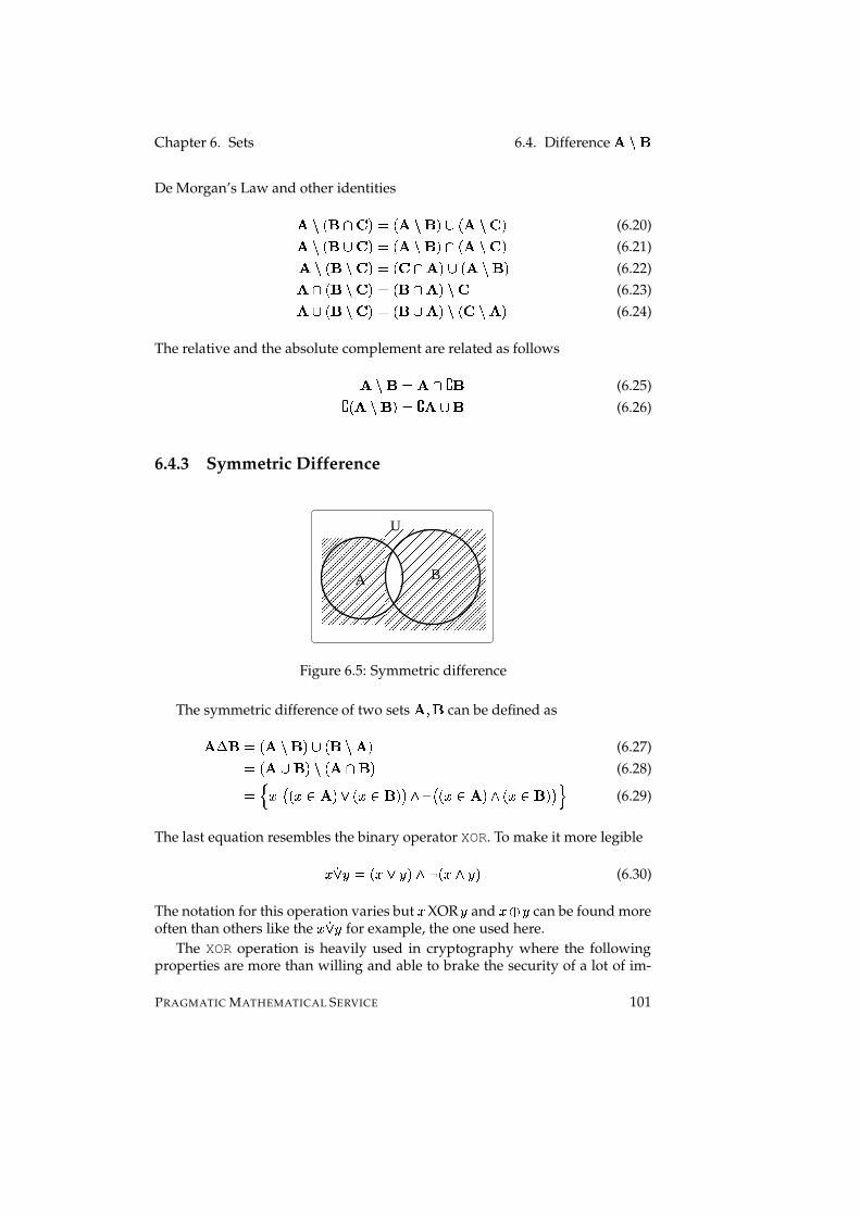
Chapter 6. Sets 6.4. Difference HRQSKDe Morgan’s Law and other identitiesH Qs��K P .Ë�{I ��H QSK���Me��HRQ�.Ë� (6.20)H Qs��K M .Ë�{I ��H QSK���Pe��HRQ�.Ë� (6.21)H Qs��K Q�.Ë�{I � .«P¸HO��Me��HRQSK�� (6.22)HNPe��K Q�.Ë�{I ��K«POHO�åQ�. (6.23)HNMe��K Q�.Ë�{I ��K«MOHO�åQs� . QSH¸� (6.24)
The relative and the absolute complement are related as followsHRQSKRI¶H PLB�K (6.25)B|��H QSKË�{ITB�H M¸K (6.26)
6.4.3 Symmetric Difference
U9U9U9U9U9U9U9U9U9U9U9UU9U9U9U9U9U9U9U9U9U9U9UU9U9U9U9U9U9U9U9U9U9U9UU9U9U9U9U9U9U9U9U9U9U9UU9U9U9U9U9U9U9U9U9U9U9UU9U9U9U9U9U9U9U9U9U9U9UU9U9U9U9U9U9U9U9U9U9U9UU9U9U9U9U9U9U9U9U9U9U9UU9U9U9U9U9U9U9U9U9U9U9UU9U9U9U9U9U9U9U9U9U9U9UU9U9U9U9U9U9U9U9U9U9U9UU9U9U9U9U9U9U9U9U9U9U9UV9V9V9V9V9V9V9V9V9V9V9VV9V9V9V9V9V9V9V9V9V9V9VV9V9V9V9V9V9V9V9V9V9V9VV9V9V9V9V9V9V9V9V9V9V9VV9V9V9V9V9V9V9V9V9V9V9VV9V9V9V9V9V9V9V9V9V9V9VV9V9V9V9V9V9V9V9V9V9V9VV9V9V9V9V9V9V9V9V9V9V9VV9V9V9V9V9V9V9V9V9V9V9VV9V9V9V9V9V9V9V9V9V9V9VV9V9V9V9V9V9V9V9V9V9V9VV9V9V9V9V9V9V9V9V9V9V9V
W9W9W9W9W9W9W9W9W9W9W9W9W9WW9W9W9W9W9W9W9W9W9W9W9W9W9WW9W9W9W9W9W9W9W9W9W9W9W9W9WW9W9W9W9W9W9W9W9W9W9W9W9W9WW9W9W9W9W9W9W9W9W9W9W9W9W9WW9W9W9W9W9W9W9W9W9W9W9W9W9WW9W9W9W9W9W9W9W9W9W9W9W9W9WW9W9W9W9W9W9W9W9W9W9W9W9W9WW9W9W9W9W9W9W9W9W9W9W9W9W9WW9W9W9W9W9W9W9W9W9W9W9W9W9WW9W9W9W9W9W9W9W9W9W9W9W9W9WW9W9W9W9W9W9W9W9W9W9W9W9W9WW9W9W9W9W9W9W9W9W9W9W9W9W9WW9W9W9W9W9W9W9W9W9W9W9W9W9WX9X9X9X9X9X9X9X9X9X9X9X9X9XX9X9X9X9X9X9X9X9X9X9X9X9X9XX9X9X9X9X9X9X9X9X9X9X9X9X9XX9X9X9X9X9X9X9X9X9X9X9X9X9XX9X9X9X9X9X9X9X9X9X9X9X9X9XX9X9X9X9X9X9X9X9X9X9X9X9X9XX9X9X9X9X9X9X9X9X9X9X9X9X9XX9X9X9X9X9X9X9X9X9X9X9X9X9XX9X9X9X9X9X9X9X9X9X9X9X9X9XX9X9X9X9X9X9X9X9X9X9X9X9X9XX9X9X9X9X9X9X9X9X9X9X9X9X9XX9X9X9X9X9X9X9X9X9X9X9X9X9XX9X9X9X9X9X9X9X9X9X9X9X9X9XX9X9X9X9X9X9X9X9X9X9X9X9X9XU
A B
Figure 6.5: Symmetric difference
The symmetric difference of two sets H©:�K can be defined asH n KRI ��HRQSK���MG��KÍQSH¸� (6.27)I ��H MOK���Qs��H POK�� (6.28)IZYA �� u ��A �iH¸�[=O�qA �iKË� w 1]\ u ��Aá�VH¸�x1O��Aá�OK�� w_^ (6.29)
The last equation resembles the binary operator XOR. To make it more legibleAa`=2Ö�I ��Aa=#Ö7��1b\±��A 1#Ö7� (6.30)
The notation for this operation varies but A XOR Ö and AdcVÖ can be found moreoften than others like the Aa`=ÈÖ for example, the one used here.
The XOR operation is heavily used in cryptography where the followingproperties are more than willing and able to brake the security of a lot of im-
PRAGMATIC MATHEMATICAL SERVICE 101
6.5. Power Chapter 6. Sets
plementations. Exchanging then
-sign with c for legibility we gete cgf IOfhc e (6.31)� e cif©�jck vI e c«�lfmck }� (6.32)� e cif©��c¶�nfock x�}I e ck (6.33)e c e ITM (6.34)e PG�nfock x�}IN� e Ppf©��c¶� e PL }� (6.35)
6.5 Power
The power set is not implemented directly in this program because the functionArray.prototype.subsets does not add the empty set to the output2. Forthe sake of completeness: the axiom of the power set isq �qH¸�}I � H � Ö � ƱÆ��OÖ ��� � � ���8�OAbà �8�OHO� (6.36)
6.5.1 Families and other Collections
The subsets of the power set form so called “families” or “collections” of sets,for example the set of all disjoint sets of some power set. The common notationis to typeset the names of these collections in Fraktura3.
For any family r r / q ��HO� (6.37)
Example: let H be a small set of integers HÓI�k / :���: � l . The power set is thenq ��HO�}I�k'MÇ:�k / l : k³� l :�k � l :�k / :4� l :�k / : � l :�k³�7: � l :�k / :��|: � lxl (6.38)
The set r of all subsets of H that have an even prime as a member isrLI k$k / l : k / :�� l :�k / : � l :�k / :��7: � l$l (6.39)
6.6 Cartesian Product 2 st4The cartesian product of two sets H©:�K is a set of ordered pairs where each pairconsists of one element from H and one from KH TOKRI k��q9:_;<�8� q ��H MOK���à 9)�VHÀ1�; �iK l (6.40)
2It is difficult to express the empty set in computerprograms, even “nothing” has to have anaddress
3The \mathfrac � letter command from the uwvyx -LATEX packet has been used here. Thefont is called eufrak—Euler Fraktur alphabet.
102 PRAGMATIC MATHEMATICAL SERVICE
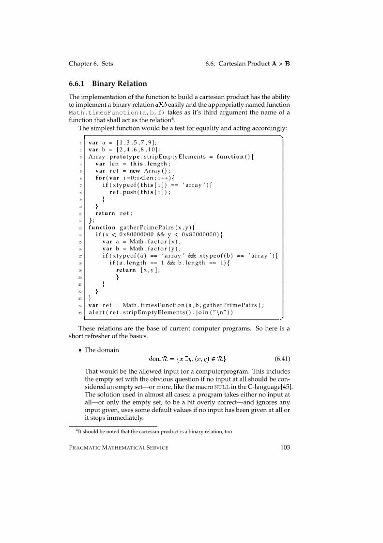
Chapter 6. Sets 6.6. Cartesian Product H TVK6.6.1 Binary Relation
The implementation of the function to build a cartesian product has the abilityto implement a binary relation 9Nz¸; easily and the appropriatly named functionMath.timesFunction(a,b,f) takes as it’s third argument the name of afunction that shall act as the relation4.
The simplest function would be a test for equality and acting accordingly:�1 var a = [ 1 , 3 , 5 , 7 , 9 ] ;2 var b = [ 2 , 4 , 6 , 8 , 1 0 ] ;3 Array . prototype . stripEmptyElements = function ( ) �4 var len = t h i s . length ;5 var r e t = new Array ( ) ;6 for ( var i =0; i � len ; i ++) �7 i f ( xtypeof ( t h i s [ i ] ) == ’ array ’ ) �8 r e t . push ( t h i s [ i ] ) ;9 �
10 �11 return r e t ;12 � ;13 function gatherPrimePairs ( x , y ) �14 i f ( x � 0 x80000000 && y � 0 x80000000 ) �15 var a = Math . f a c t o r ( x ) ;16 var b = Math . f a c t o r ( y ) ;17 i f ( xtypeof ( a ) == ’ array ’ && xtypeof ( b ) == ’ array ’ ) �18 i f ( a . length == 1 && b . length == 1) �19 return [ x , y ] ;20 �21 �22 �23 �24 var r e t = Math . t imesFunct ion ( a , b , gatherPrimePairs ) ;25 a l e r t ( r e t . stripEmptyElements ( ) . j o i n ( ” s n” ) ) �These relations are the base of current computer programs. So here is a
short refresher of the basics.� The domain a &$�Az�I k�A2à � Ö�:³��A�:4Ö7�8�{z l (6.41)
That would be the allowed input for a computerprogram. This includesthe empty set with the obvious question if no input at all should be con-sidered an empty set—or more, like the macro NULL in the C-language[45].The solution used in almost all cases: a program takes either no input atall—or only the empty set, to be a bit overly correct—and ignores anyinput given, uses some default values if no input has been given at all orit stops immediately.
4It should be noted that the cartesian product is a binary relation, too
PRAGMATIC MATHEMATICAL SERVICE 103
6.6. Cartesian Product H TOK Chapter 6. Sets� The range W_�� |z�I k�Ö�à � Aå:³��A�:4Ö7�8�{z l (6.42)
For a computer program: the output it is able to give.� The field } ã � a zÓI a &��iz MÜW��! ~z (6.43)
The fields a current computer program can use are finite subsets of Z .� The inverse z ® " I k���Öö:�A���à���A�:4Ö7�%�{z l (6.44)
That is the “back” in “back&forth” it is the “forth”.� The image of a set Hz�� H)�*I�k³Ö.� W��! |zGà � A��VHF:���Aå:4Ö7�8�{z l (6.45)� The image of a set H under the inverse of a relation z , also known as the“preimage” z ® " � H �öI k�A � a &$�AzGà � Ö.�VH©:³��Aå:�Ö7�%�{z l (6.46)
So a relation z is a relation on H if} ãF� a z /�H (6.47)
It is desirable to keep �ÕH , the number of elements of H , as small as possibleand moreso that
} ã � a zJI¶H or the program might not be fully testable. It willdefinitly not be fully testable if à HGà ¾ à W±à even with infinite Turing machines 5.
Complicated looking formulas for which a simple example is advised.Consider æ ��A��{I¶A $ which maps the real line to itself æ"� [ à [ .� The domain is [� The range is [ �� The field is [� The inverse is æ ® " ��A��xI . A . That means that6æ ® " �}k � l �@I k(w / : / l (6.48)æ ® " �4��)!: / �°�{I �°w . / :�w6)³�*Me�°)(: . / � (6.49)æ ® " �}k(w6) l �{IKM (6.50)
5Under the assumption, of course that the number of steps of a Turing machine is at mostcountable.
6The parentheses anotate a range of numbers, in the case of Çqß)� ÿ Ê it is the set ��ß)� ¦ ¦ ¦�� ÿ ����� Ç��(Ê .104 PRAGMATIC MATHEMATICAL SERVICE

Chapter 6. Sets 6.6. Cartesian Product H TVKSo domain, range and field of æ ® " ��A�� area &$� æ ® " I«[ � (6.51)W��! æ ® " I«[ (6.52)} ã � a æ ® " I«[ � MO[LI¶[ (6.53)� The image is the “result” of æ ��A�� for every AN� a &$� æ ; it is the range of æor the image of a &�� æ .
im k / : � l I æ � k / : � l �{I k � :�) ì l (6.54)
im æ I«[ � (6.55)� The preimage is, by the definition of the image and the definition of theinverse, the image of W��! æ .
im
® " k � :�) ì l I æ® " � k � :�) ì l �{I k(w � :�w / : / : � l (6.56)
im
® " æ I¶[ (6.57)
With a function æ"� e à7f , the sets k p " : p $ : ����� : p C l / e and k � " : � $ : ����� : � C l /f the following (in)equalities should look familiar to the reader.æ � p C M p E �}I æ � p C �*M æ � p E � (6.58)æ ® " � � C M � E �}I æ ® " � � C �*M æ ® " � � E � (6.59)
but æ � p C P p E � / æ � p C �*P æ � p E � (6.60)æ ® " � � C P � E �}I æ ® " � � C �*P æ ® " � � E � (6.61)
From the example with æ ��A��±I A $ it should be obvious that æ ��A�� is not alwayssimply the inverse of æ ® " ��Aö� for every Aæ � æ ® " � � C ��� / � C (6.62)æ ® " � æ � p C ���|� p C (6.63)
The average computer language designer has problems with the empty setas described above, so to avoid it the mapping æ shall be extended to æ�� \ à \because the square root is well defined for every Aá�V\ .a &$� æ I«\ (6.64)a &$� æ ® " I«\ (6.65)W��! æ I«\ (6.66)W��! æ ® " I«\ (6.67)
PRAGMATIC MATHEMATICAL SERVICE 105

Chapter 7
Combinatorics
106

Chapter 8
Statistical Functions
It is easy to lie with statistics. It is hard to tell the truth withoutstatistics. [ANDREJS DUNKELS]
He uses statistics as a drunken man uses lampposts—forsupport rather than illumination. [ANDREW LANG]
8.1 Distributions
Some basic algorithms for the most common distributions are implemented;least the probability function and the distribution function, but also the inverseof the distribution function for almost all of the offered distributions.
8.1.1 Beta Distribution
The beta distribution is based on the beta function� ��9�:�;��{I =x��9|�°=x�q;<�=}��96rt;<� (8.1)
Probability Function
The probability function �UWÁ��Aå:�9�:_;<� is implemented for 9.(���:�; (���:�� nAá )�dWÁ��Aå:�9�:_;<�{ILA ¡³® " �°)²wyA�� ;xwt)´�� ��9�:_;<� (8.2)
Distribution Function
The distribution function¦ W ��A�:�9�:�;�� is implemented for 9.(���:�; (t�7:�A (��¦ W ��Aå:�9�:_;<�{I _ ) if 9.(��Ì1Ë; (�� 1~A ¾ )���Aå:�9�:_;<� otherwise
(8.3)
107

8.1. Distributions Chapter 8. Statistical Functions
where ����A�:�9�:�;�� is the regularized beta function.
8.1.2 Binomial
Probability Function
The probability function � 9 ���@:_òö: � � is implemented in two different ways for�G�VWS:�� � � � ) . � 9 ���@:�òö: � �{I ð � ò ñ � ï �°)�w � � C ® ï (8.4)
where u C ï w is the binomial coefficient calculated with factorials, following thetextbook. The other implementations uses the logarithm of the binomial coef-ficient calculated with the log-Gamma function.�� ©ð � ò|ñ I �� �=#���#rL)´�Èw���� �=#�qò~r¶)³��r �� �=µ���¸w¬ò6rL)´�4� (8.5)
This second implementation returns the logarithm of the binomial probabilityfunction �5 X� 9 ���@:�òö: � ��5 X� 9 ���@:_òö: � �{I �5 ©ð � ò�ñ rnò8�5 � r«���Vwyò��!�� ��°)²w � � (8.6)
Distribution Function
The distribution function¦ 9 ���@:_òö: � � for � � � � ) is implemented with the
help of the regularized beta function.¦ 9 ���@:_òö: � �{I¶���°)²w � :_òÇwZY��O[{:�)xr Y �O[´� (8.7)
8.1.3 Cauchy
Probability Function
The probability function � E ��Aå: � : R � for R ¾ � is� E ��Aå: � : R �xI )�4)xr Ò!®��� $ � �ëR (8.8)
Distribution Function
The distribution function¦ E ��Aå: � : R � for R ¾ � is¦ E ��A�: � : R �xI )/ r �����! u Ò!®��� w� (8.9)
108 PRAGMATIC MATHEMATICAL SERVICE

Chapter 8. Statistical Functions 8.1. Distributions
Inverse of the Distribution Function
The inverse of the distribution function¦ ® "E ��Aå: � : R � for R ¾ ��:�� �ÍA � ) can
be represented in closed form¦ ® "E ��A�: � : R �SI ¹º» º¼w g if A¸I«�règ if A¸IN)� w R %<&��´��A � � else
(8.10)
8.1.4 F-Distribution
Probability Function
The probability function � i ��Aå:3%G:��å� for A�(t�7:3% (t��:4�N(t� is implemented as� i ��A�:7%e:4�å�}I ã�äæå ð51 % / w�) 2 �� 1 %OA� 2 w % r¬�/ �5 1 )xr %OA� 2 ñ u E C w�u E $ : C $ w(8.11)
Distribution Function
The distribution function¦ i ��Aå:3%G:��å� for A`( ��:7% (Í�7:4� ( � is implemented
as � i ��Aå:7%e:4�å�xI _ ) if A¸I règ)²wy� 1 "" � E Ò 6 C ¯ : C $ : E $ 2 else(8.12)
where ���Ahw�9:_;<� is the regularized beta function.
Inverse of the Distribution Function
The inverse of the distribution function¦ ® "i ��Aå:7%e:4�å� for � ��A � )(:7% (Ô�7:���(� can be represented in closed form¦ ® "i ��Aå:3%G:��å�år ¹» ¼ règ if A¸Iè))¦ ® "W u )²wGA�: C $ : E $ w CE else (8.13)
where¦ ® "W is the inverse of the beta distribution function.
8.1.5 Geometric
Probability Function
The probability function � ç ��A�: � � for ��� � � )(:4A �VW is implemented as� ç ��Aå: � �{I _ ) if AOI règ 1 � IL�� �4)²w � � Ò else(8.14)
PRAGMATIC MATHEMATICAL SERVICE 109
8.1. Distributions Chapter 8. Statistical Functions
Distribution Function
The distribution function¦ ç ��Aå: � � for ��� � � )!:�A �OW is implemented as¦ ç ��A�: � �xI _ ) if A¸I règ 1 � I¶�)²wÔ�°)�w � � Ò³� " else
(8.15)
Inverse of the Distribution Function
The inverse of the distribution function¦ ® "ç ��Aå: � � for � �LAG�Í)!:��)� � �Í) can
be represented in closed form¦ ® "ç ��A�: � �xI _ règ if AOIÍ)���xä 1j� 8 : " ®�Ò ¯8 : " ® K ¯�� w�)!:�� 2 else(8.16)
where ���xä*�q9�:�;<� denotes the maximum value of the two variables 9�:�; .8.1.6 Hypergeometric
Probability Function
The probability function ���Ç��Aå:7%e: ��:��å� for kã%e:4�@: � l �GWS:4� HIÍ��:7% �¬��:�� �¬� isimplemented as���Ç��Aå:3%G:=��:4�å�{I ¹» ¼ � if A H�VW 1OA�(�%Z1~�N tA�1²���OwGAö�%(Í�V�Èw %i���� º �<��� � �S � º �� �S � else
(8.17)
Distribution Function
The distribution function¦ �Ë��A�:7%e: ��:4�å� for kq%G:��@: � l �VWS:�� HI«�7:3% � ��:��G� � is
implemented by means of the distribution function of the discrete distribution.¦ �Ë��A�:7%e: ��:��å�{I ¦]� ��A�:����°� C� � " :=���Ë���_:7%e: ��:��å� C� � " � (8.18)
This might be one of the cases, where the code of the implementation is morereadable as the underlying algorithm.
Inverse Distribution Function
The inverse distribution function is similar to the distribution function exceptthat it uses the inverse distribution function of the discrete distribution insteadof the normal distribution function.
The inverse distribution function¦ ® "� ��Aå:3%G:=��:4�å� for kq%G:��@: � l � WS:4� HI�7:3%O� ��:4� � � is implemented by means of the distribution function of the
discrete distribution.¦ ® "� ��Aå:3%G:=��:4�å�}I ¦ ® "� ��A�:����°� C� � " :=���Ë���_:7%e: ��:��å� C� � " � (8.19)
110 PRAGMATIC MATHEMATICAL SERVICE

Chapter 8. Statistical Functions 8.2. Means
8.2 Means
Let 1 be a sequence k³9 � l C� � " of data points, for example the content of the au-
thor’s ashtray after he gave up cigarette smoking—a handful of coins of differ-ent values: �iI¶õ (8.20)k³9 " :�9 $ : ����� :�9 C l I k��q� � �7)!:_ó!�<:���� � � / :�õ(��:³��� � ��ó|:�����:³��� � )���: / �!��: (8.21)��� � / �7:�)³ó!�<:��q� � ó��7: / )´��:��4) � �!��: � �<:�� /|� �!�|:��(� lSuch a sequence can be described in several ways.
8.2.1 Range
The range W_�� ��z1{� of a dataset 1 is the difference between the smallest and thelargest element. W_�� ��q1}�{I ��� ä*�q1}�2wG��35 å�q1}� (8.22)
8.2.2 Harmonic Mean
The harmonic mean Dn�q1{� is defined byDn�q1{�{I �F C� � " "¡)� (8.23)
8.2.3 Geometric Mean
The geometric mean0 �z1{� is defined by0 �z1{�{I * C�� � " 9 � + )� (8.24)
With only two elements in the sequence ( �eI / ) the geometric mean is relatedto the arithmetic mean
p �z1{� and harmonic mean Dn�q1{�0 �q1{�{I p �q1}�°Dv�z1{� (8.25)
As every mean is a special case of the general power mean, the geometric meanis the case
� ? of the power mean. The geometric mean is, the name impliesit, describable by geometric means and is thus one of the three Pythagoreanmeans.
The following might be of additional interest ([44])0 ��9 " rnu�:�9 $ rnu�: ����� :�9 C rnu���(±u}r 0 ��9 " :�9 $ : ����� :�9 C � (8.26)
PRAGMATIC MATHEMATICAL SERVICE 111

8.2. Means Chapter 8. Statistical Functions
8.2.4 Root-Mean-Square
The root-mean-square ù ! ~*�q1}� is defined for a discrete distribution byù ! ~��q1{�}I ���� * C� � � " 9 $� + )� (8.27)
and for a continuous distribution byù ! ~*�q1}�{I�� K ����9|�°9 $ a 9K ����9|� a 9 (8.28)
It has been shown by [44] that for a positive constant uù ! ~��q9 " rvu�:�9 $ rvu�: ����� :�9�C~rnu��� �u{rÁù ! ~*�q9 " :�9 $ : ����� :�9�C7� (8.29)
8.2.5 Arithmetic Mean
The arithmetic mean is probably the most common mean, taught in primaryschool and called the average. The arithmetic mean
p �z1{� is defined byp �z1{�}I * C� � � " 9 � + )� (8.30)
Similar to the geometrical mean [44] showedp �q9 " rvu�:�9 $ rvu�: ����� :�9 C rnu���Isu{r p ��9 " :�9 $ : ����� :�9 C � (8.31)
8.2.6 Logarithmic Arithmetic Mean
The logarithmic arithmetic mean
p !@�q1}� is defined byp !@�q1}�{I * C� � � " �5 �9 � + )� (8.32)
8.2.7 Power Mean
The power mean is the generalized algorithm for means. Every other meancan be derived from the power mean. It is defined by� K �q1{�{I * )� C�� � " 9 K � + )� with 9 ï ¾ � (8.33)
If we include maximum and minimum as means and denote the power meanas� K the special cases of the power mean are
112 PRAGMATIC MATHEMATICAL SERVICE
Chapter 8. Statistical Functions 8.2. Means���Common Symbol Name of Mean� ® î ��3� Minimum� ® " D Harmonic Mean� ? 0
Geometric Mean� " pArithmetic Mean� $ ù ! ~ Root-Mean-Square� î ���xä Maximum
8.2.8 Arithmetic Geometric Mean
This mean is actually a limit. The recurrence formulae forã�� ! ��9�:�;<� are9�C � " I )/ ��9�C~rn;�C7� with 9�?ÁI«9 (8.34); C � " I 9 C ; C with ; ? I¶; (8.35)
(8.36)
The mean is reached when 9|C©I ;�C but in praxi the iterating takes forth until9�C#IÍ;�C~rtu or 9�C~rtuÁIè;<C where u is an arbitrary small constant—the desiredprecision for the numerical solution.
Some combinations of 9 and ; have a closed form for� ! �q9�:�;<� for example
the famous Gauss constant. The Gauss constant is the reciprocal ofã�� ! �°)(: . / �)ã�� ! �°)!: . / � I � = u "À w � $/ � ê 6 $ . / (8.37)
The derivative�� ; ã�� ! �q9�:�;<�{I �õ ¡³® 9¡�� 9�; ë ��9ËI«;<�æcÁ� ¡³® 9¡�� 9 �@w / ;� Ç� ¡³® 9¡�� 9 �A �� ¡³® 9¡�� 9 � B $ (8.38)
where ���Aö� is the complete elliptic integral of the first kind and c���A�� is that ofthe second kind.
For the special case ofã�� ! �°)!:_;<� a series expansion existã�� ! �4)!:_;<�{Ièw �/ �� u "À ; w r � � )}r`�5 u "À ; w � ; $õ � �5 u "À ; w � $ r-� u ; À w (8.39)
Some properties ofã�� ! �q9:_;<�u ã�� ! ��9�:_;<�{I ã�� ! ��u<9�:�u�;<� (8.40)ã�� ! ��9�:_;<�{I ã�� ! ð )/ ��96rn;���: . 9|; ñ (8.41)ã�� ! 1�)(: )²wGA $ 2VI ã�� ! �°)xrvAå:�)�wGAö� (8.42)ã�� ! �4)!:_;<�{I )xrt;/ ã�� ! * )!: / . ;)xrn; + (8.43)
PRAGMATIC MATHEMATICAL SERVICE 113
8.2. Means Chapter 8. Statistical Functions
8.2.9 Geometric Harmonic Mean
This mean is the limit of the recurrence formulae9 C � " I / 9 C ; C9�C6rt;�C with 9 ? I¶9 (8.44); C � " I 9 C ; C with ; ? I ; (8.45)
It is implemented in a slightly different way9�C � " I /"¡ S r "9 S with 9�?ÁILDv�z1{� (8.46);�C � " I 9�C�;�C with ;_?ÁI 0 �q1{� (8.47)
with the sum "¡ S rÏ"9 S HI � , Dv�z1{� the harmonic mean and0 �q1{� the geometric
mean. The mean is reached when 9|C�I«;�C but in praxi the iterating takes forthuntil 9�CvIJ;<C�r¶u or 9�C�r¶u#I ;�C where u is an arbitrary small constant—thedesired precision for the numerical solution. The geometric harmonic mean0 �Ç�z1{� is related to the arithmetic geometric mean
ã�� ! by0 ���z1{�{I��53��C�� î 9 C I )ã�� ! 1Õ"¡ & :±"9 & 2 (8.48)
8.2.10 Arithmetic Harmonic Mean
The arithmetic harmonic mean is identical to the geometric mean. The recur-rence formulae are 9�C � " I )/ �q9�C~rt;�C7� with 9�?ÁI¶9 (8.49); C � " I / 9 C ; C9�C6rn;�C with ; ? I ; (8.50)
Calculating the limits 9�:�;Càâg givesp � �z1{�{I��53��C�� î 9�C�IO��3#�C$� î ;�C�I . 9|; (8.51)
which is indeed the geometric mean.
8.2.11 Weighted Geometric Mean
The weighted geometric mean0¢¡ �q1{� puts a value � C4�nW to each element of
the sequence 9�C . 0£¡ �q1{�xI F C� � " � C �� �9 CF C� � " � C (8.52)
withF C� � " � C Iè)
114 PRAGMATIC MATHEMATICAL SERVICE

Chapter 8. Statistical Functions 8.2. Means
8.2.12 Weighted Arithmetic Mean
The weighted arithmetic mean
p ¡ �q1}� puts a value � CN�vW to each element ofthe sequence 9�C .
p ¡ �q1{�{I F C� � " � C|9�CF C� � " � C (8.53)
withF C� � " � C�Iè)
8.2.13 Weighted Harmonic Mean
The weighted harmonic mean D ¡ �z1{� puts a value � C �tW to each element ofthe sequence 9 C . D ¡ �q1{�{I F C� � " ¡ S¡ SF C� � " � C (8.54)
withF C� � " � C Iè)
8.2.14 Pythagorean Means
a cb
GH
A
Figure 8.1:
p �q9�:�;<� ¾ 0 ��9�:�;�� ¾ Dv�q9�:�;<�The group of the arithmetic mean
p �q1{� , geometric mean0 �z1{� and har-
monic mean Dv�q1{� are also called the Pythagorean means. The relation between
PRAGMATIC MATHEMATICAL SERVICE 115
8.2. Means Chapter 8. Statistical Functions
them in case of positive arguments 9�:�; (Ô� isp �q1}� ¾ 0 �z1{� ¾ Dv�q1{� (8.55)
The inequality is shown geometrically in figure 8.1.
8.2.15 Median
The median "76 $ is the value in the middle of a sorted sequence 1 with length� and defined by "36 $ I ¹» ¼¤ 9 C 6 $)¥ æ � * & a,a ���å�¡ S§¦ ÷ � ¡©¨ S + ä�ª ¦ ÷$ æ � * ãã�$ã� ����å�(1Ç� HI¶� (8.56)
The efficiency of the median depends on the sample size z I / �irè) by theway of ([50]) �53��« � î � �� � / �#r¶)³� I /� (8.57)
8.2.16 Mode
The mode is the number of occurances of one value. In the case of the changein the ashtray the mode is either ��� � ó!�7: / )³� (unimodal) or all of the elements(multimodal1). Only the unimodal mode is implemented directly.
8.2.17 Variance
The bias corrected sample variance R $ is defined byR I F C� � " ��9�CËw p �q1{��� $�Owt) (8.58)
where
p �q1{� is the arithmetic mean.
8.2.18 Logarithm of the Variance
The logarithm of the bias corrected sample variance R $� is defined byR � I F C� � " �V�5 �9�CÕw p �Þ1{�4� $�Vw�) (8.59)
where
p �q1{� is the arithmetic mean
1That is, of course, not the exclusive name for “all elements occur the same number of times”,only to distinguish from unimodal. There are distinct names for special values of multimodalityin the literature like “bimodal”, “trimodal” and so on.
116 PRAGMATIC MATHEMATICAL SERVICE
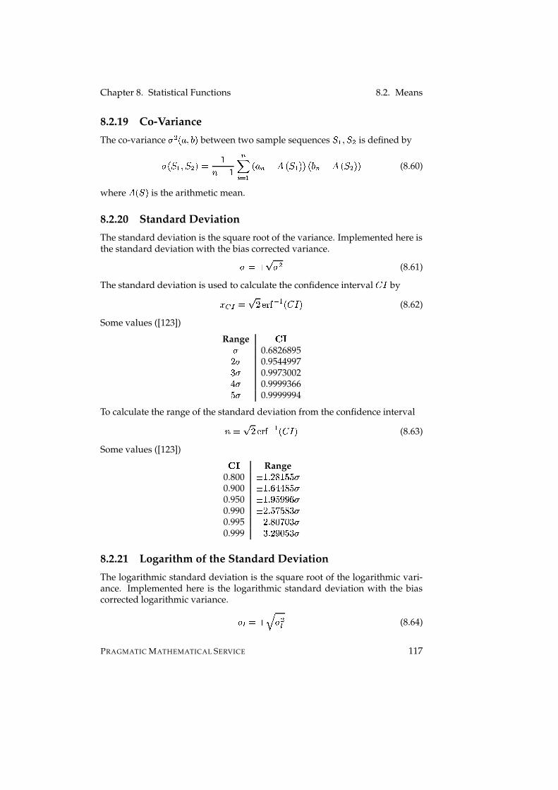
Chapter 8. Statistical Functions 8.2. Means
8.2.19 Co-Variance
The co-variance R $ ��9�:_;<� between two sample sequences 1 " :�1 $ is defined byR �z1 " :_1 $ �xI )�Ow�) C� � � " �q9 C w p �z1 " �4���z; C w p �q1 $ ��� (8.60)
where
p �z1{� is the arithmetic mean.
8.2.20 Standard Deviation
The standard deviation is the square root of the variance. Implemented here isthe standard deviation with the bias corrected variance.R I r . R $ (8.61)
The standard deviation is used to calculate the confidence interval/ � byA Ej¬ I . / ããW7V ® " � / ��� (8.62)
Some values ([123])
Range .�R 0.6826895/ R 0.9544997� R 0.9973002� R 0.9999366ó R 0.9999994
To calculate the range of the standard deviation from the confidence interval�VI . / ã»W3V ® " � / ��� (8.63)
Some values ([123]) .� Range0.800 P ) � / õ7)´ó!ó R0.900 P ) � ì �!� õ(ó R0.950 P ) � ��ó��(� ì R0.990 P /7� ó�í�ó!õ!� R0.995 P /7� õ(��í��!� R0.999 P � � / �!��ó�� R
8.2.21 Logarithm of the Standard Deviation
The logarithmic standard deviation is the square root of the logarithmic vari-ance. Implemented here is the logarithmic standard deviation with the biascorrected logarithmic variance. R � I r « R $� (8.64)
PRAGMATIC MATHEMATICAL SERVICE 117

8.2. Means Chapter 8. Statistical Functions
8.2.22 Average Deviation
Also known as mean deviation R E it is defined byR E I )/ C� � � " à 9 � wp �q1{��à (8.65)
where
p �q1{� is the arithmetic mean.
8.2.23 Geometric Standard Deviation
The geometric standard deviation R �R � I ã ä!å �� ���� )� C� � � " �V�5 �9 � wG�5 0 �q1}�4� $ �� (8.66)
where0 �z1{� is the geometric mean.
8.2.24 Skewness
The skewness & is defined differently in different sources, the variation imple-mented is &FI F C� � " ��9 � w p �z1{�4� ê���¸w�)³� p ê �z1{� (8.67)
where
p �q1{� is the arithmetic mean.
8.2.25 Kurtosis
The kurtosis is measured in two different ways: one is called “kurtosis proper”& $ and the other “kurtosis excess” � $ ([1]). The difference is � 2. It is imple-mented as & $ I F C� � " ��9 � w p �z1{�4� À�q�¸w�)³� p À �z1{� (8.68)
� $ I F C� � " ��9 � w p �z1{�4� À�q�¸w�)³� p À �z1{� wy� (8.69)
8.2.26 Other Means
Other means, beside the obvious “money” and “blunt object” exists. One ofthese is the Stolarsky mean 1åC ([102])1 f �q9�:�;<�{I ð 9 f wy; f* ��9Çwy;���ñ ä· � ä (8.70)
2Yes, really!
118 PRAGMATIC MATHEMATICAL SERVICE

Chapter 8. Statistical Functions 8.2. Means
This mean is not implemented but the following ECMA-script code might givean idea. �
1 function s t o l a r s k y ( a , b , r ) �2 / / S a n i t y c h e c k s o m i t t e d h e r e3 var nominator = Math .pow( a , r ) � Math . pow( b , r ) ;4 var denominator = r � ( a � b ) ;5
6 return Math .pow( nominator/denominator , 1 / ( r � 1) ) ;7 � ; �
The Stolarsky mean is derived from the mean value theorem�® �4� Aå:4Ö�� æ â � ® �}I æ ��A��2w æ ��Ö7�AµweÖ (8.71)
Solving for
®gives
® I æ â ® " ð æ ��Aö�2w æ ��Ö7�AµwGÖ ñ (8.72)
Or in a more generalized form for �µrL) variables with the nth derivative1 f �q9 " :�9 $ : ����� :�9 C � " �}I æ C � ä ���@é æ ��9 " :�9 $ : ����� :�9 C � " ��� (8.73)
Some relations to other means
Stolarsky Mean Related Mean�53�� f � ® î 1 f ��9�:�;<� Minimum1 ® " ��9�:�;�� Geometric mean��3#� f �,? 1 f �q9:_;<� Logarithmic mean ( æ ��A��{I¬�� ²A )1 ä÷ �q9:_;<� Power mean with exponent "$��3#� f � " 1 f �q9:_;<� Identric3 mean ( æ ��Aö�{ILAX�5 ²A )1 $ ��9�:�;<� Arithmetic mean�53�� f � � î 1 f ��9�:�;<� Maximum
And as we are at it, the identric mean ����9�:_;<� mentioned in the table 8.2.26 isdefined by ����9�:�;��{I )0b¯ �N°\ 9 ¡; 9 (8.74)
The identric mean is not implemented but this short ECMA-script should givean idea. �
1 function i d e n t r i c ( a , b ) �2 / / S a n i t y c h e c k s o m i t t e d h e r e3 var nominator = Math .pow( a , a ) ;4 var denominator = Math .pow( b , b ) ;5 var r e c i p r o c a l E = 1/Math . E ;6
PRAGMATIC MATHEMATICAL SERVICE 119

8.2. Means Chapter 8. Statistical Functions
7 return r e c i p r o c a l E � Math .pow( nominator/denominator , a� b ) ;8 � ; �
Generalization to more then the mere two variables follows, like the generaliza-tion of the Stolarsky mean, by the mean value theorem for divided differences.
The identric mean has caught some interest from [3, 18], just to name two.
120 PRAGMATIC MATHEMATICAL SERVICE
Chapter 9
Physics Functions
9.1 Astronomy
9.2 Mechanics
9.3 Quantum Mechanics
9.4 Thermodynamics
9.5 Electric
9.5.1 Capacitance of a Cylinder Capaciator (Coax-cable)
121

Chapter 10
String Functions
10.1 Comparing
10.1.1 Similarity (Ratcliff/Obershelp)
10.1.2 Difference (Levenshtein)
10.2 Sampling
10.3 Mixing
122

Chapter 11
Helper Functions
11.1 Lists (Arrays)
123

Chapter 12
Miscellaneous Functions
12.1 ±12.1.1 Size of a Bloomfilter
12.1.2 Happy Numbers
A positive integer is a happy number if the sum of the squares of its digits—iterated—reaches ) .
Let ' be a concatenation j " ë�ë�ë j C of decimal digits j C �Nk³��:�)!: / :��7: � :�ó7: ì :�í�:�õ7:�� l ,then the reccurence formula
j â " ����� j âC� I j $ " rLë�ë�ë j $C (12.1)
reaches one of the points k³��:�)(: � :�) ì : / ��:���í�: � / :_ó�õ7:�õ��7:�) � ó l ([84]). For '6IÍ��í thecalculation is )��(�,I«� $ r�í $ (12.2))��~IN) $ rn� $ rn� $ (12.3))�IN) $ rn� $ (12.4)
so ��í is a happy number, but ) ì / I«� $ rn� $ (12.5)� )�IN) $ r ì $ r / $ (12.6))´í,I � $ r¶) $ (12.7)ó��~IN) $ r�í $ (12.8)/ ó6I ó $ rn� $ (12.9)/ �~I / $ rtó $ (12.10)õ(ó6I / $ rn� $ (12.11)õ!�~I«õ $ rtó $ (12.12)
124

Chapter 12. Miscellaneous Functions 12.1. WSo �(� is not a happy number and therefore called, admittedly not very inven-tive, an unhappy number. These unhappy numbers never reach ) but end inperiodical sequences. Carrying on with the example �!� at the state õ!�
) � ó6I¶õ $ rv� $ (12.13)� / Iè) $ r � $ rnó $ (12.14)/ �~I � $ r / $ (12.15)� I / $ rv� $ (12.16)) ì I � $ (12.17)��í,Iè) $ r ì $ (12.18)ó!õ~I¶� $ rtí $ (12.19)õ(�~I«ó $ rvõ $ (12.20)
the period is²´³ à � / à / �Qà � àc) ì à ��í à ó�õQà ²´³ à � / à / �Qà � àcë�ë�ë (12.21)
The numbers listed in the set k � :�) ì : / �7:���í|: � / :�ó!õ7:�õ!�7:�) � ó l end all in a periodicalsequence when used as a startvalue for formula 12.1. Only the numbers � and) from the set k´�7:�)(: � :�) ì : / �7:���í�: � / :_ó�õ|:�õ!�|:�) � ó l consolidate. The number � isexcepted from the rule because the only number that consolidates at � is � itself.
Happy Bases
Happy number exist in other bases, too. There are even happy bases like base-2and base-4, where all numbers are happy.
12.1.3 Roman Numbers µ Arabic Numbers
The main difference between the base-5 Roman system and the base-10 Arabicsystem is the lack of a symbol for zero in the Roman system.
The implementation is restricted to positive integers between 1 andì �(�!�
PRAGMATIC MATHEMATICAL SERVICE 125

12.2. Y Chapter 12. Miscellaneous Functions
12.1.4 Factorizing
12.2 ¶12.3 ·12.3.1 Greatest Common Denominator
12.3.2 Least Common Multiple
12.3.3 Basic Operations
12.4 ¸12.4.1 Rounding & Truncating
d
Figure 12.1: � � �It is not possible to represent all numbers in all possible number systems
with a finite number of symbols, so it is sometimes necessary to round thisnumber to make it representable in the number system of choice. Let the setk³��: ����� :���: � l be the alphabet ¹ with which we want to represent the number � ,
126 PRAGMATIC MATHEMATICAL SERVICE
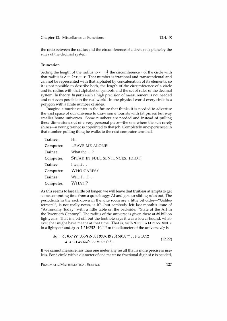
Chapter 12. Miscellaneous Functions 12.4. [the ratio between the radius and the circumference of a circle on a plane by therules of the decimal system:
Truncation
Setting the length of the radius to * I "$ the circumference u of the circle withthat radius is uÇI / * � I � . That number is irrational and transcendental andcan not be represented with that alphabet by concatenation of its elements, soit is not possible to describe both, the length of the circumference of a circleand its radius with that alphabet of symbols and the set of rules of the decimalsystem. In theory. In praxi such a high precision of measurement is not neededand not even possible in the real world. In the physical world every circle is apolygon with a finite number of sides.
Imagine a tourist center in the future that thinks it is needed to advertisethe vast space of our universe to draw some tourists with fat purses but waysmaller home universes. Some numbers are needed and instead of pullingthese dimensions out of a very personal place—the one where the sun rarelyshines—a young trainee is appointed to that job. Completely unexperienced inthat number-pulling thing he walks to the next computer terminal.
Trainee: Hi!
Computer: LEAVE ME ALONE!Trainee: What the . . . ?
Computer: SPEAK IN FULL SENTENCES, IDIOT!Trainee: I want . . .
Computer: WHO CARES?Trainee: Well, I . . . I . . .
Computer: WHAT!?
As this seems to last a little bit longer, we will leave that fruitless attempts to getsome computing time from a quite buggy AI and get our sliding rules out. Theperiodicals in the rack down in the ante room are a little bit older—“Galileoretracts!”, is not really news, is it?—but sombody left last month’s issue of“Astronomy Today” with a little table on the backside: “State of the Art inthe Twentieth Century”. The radius of the universe is given there at �(� billionlightyears. That is a bit off, but the footnote says it was a lower bound, what-ever that might have meant at that time. That is, with � � ì �xí��(� � í / ó�õ��}õ��!�Ì%in a lightyear and º©» 7 ) � ì ) ì / ó / ë�)³� ® ê � % the diameter of the universe j¼ is
j¼ I � ó ì ó�í / ��í2�(ó!õ@�(ó�ó@� ì �@�!�!õ{� � � / ì � ó�� � õ(í!í2ó!�|) � í � �!ó /��)�� ì / � � ì �}ó(ó(í ì �(ó@õ|) � / )³í½º�» (12.22)
If we cannot measure less than one meter any result that is more precise is use-less. For a circle with a diameter of one meter no fractional digit of � is needed,
PRAGMATIC MATHEMATICAL SERVICE 127

12.4. [ Chapter 12. Miscellaneous Functions
for a circle with a diameter of 10 meters two fractional digits are needed butalso for * Ièó and one digit for * I / , so to get maximal precision the numberof fractional digits needed is the number of digits of the next decimal exponent.� d I¿¾ �5 / *�5 6)���À rL) (12.23)
So a mere 63 digits of � are needed to calculate the circumference of the uni-verse as exact as physically possible.� � ê I¶� � ) � )�ó�� / ì ó!�}ó�õ(�}í���� / �!õ � ì / ì � �@�!õ!� / í��}ó�� / õ(õ � )���í) ì �{�!�(�{��í!ó±)���ó2õ / �}�(í � � �(� ó�� / (12.24)
This gives the resultu ¼ IN) � � � � ì{ì / �{� / �±)�õ��±)³�|)åõ|) ì í!í / õ � í / � / ó��|) ì � õ@� / �� ��ó@õ!õ(�}ó � � ì ��)åó ��� ó ì í /!/ �{���!�jº�» (12.25)
A 63-digit number will probably impress a lot of potential tourists and weshould not be too mannerless and give the envelope—that with the calcula-tion on its backside—to the sobbing picture of misery in the corner: the poorboy formerly known as the BEST APPRENTICE IN THE UNIVERSE; at least to hismother.
A decimal number A will be truncated � digits to result in the new numberA â A â I _ Aµw W;ã � u Ò" ? S w for A �OYAµw W;ã � 1 Ò ää & S 2 for A � (12.26)
where W;ã �i� K L�� is the remainder of the division K L . Examples:) / �(�!�!�,I���WÂÁ7 %!�°) / � � ó ì :���� (12.27)ì ó � � �6I���WÂÁ7 %!� ì ó � � � / )!: / � (12.28)
Rounding
After careful lecture of section 12.4.1 the attentive reader has most probablyobserved the problems of the calculations in that section. In the case of theuniverse the result with truncated � gives a polygon with a circumferencethat is obviously smaller than the circumference of the universe and it remainssmaller, no matter which length º©» has and after which digit � is truncated1.The tourist center is saved from a lawsuit for “Exaggerated Advertising” butthat will not help us to resolve the problem of underestimating the real size ofthe universe—especially if we get paid for the meter.
“Meter” is a good keyword. For example the price of the gasoline the au-thor’s car needs to run its motor costs at the day of the writing ) � ì �!� EUR per
1Actually, the circumference of the polygon is equal to the circumference of the universe ifÃÂÄ Ø ¥ and Ï is not truncated at all.
128 PRAGMATIC MATHEMATICAL SERVICE
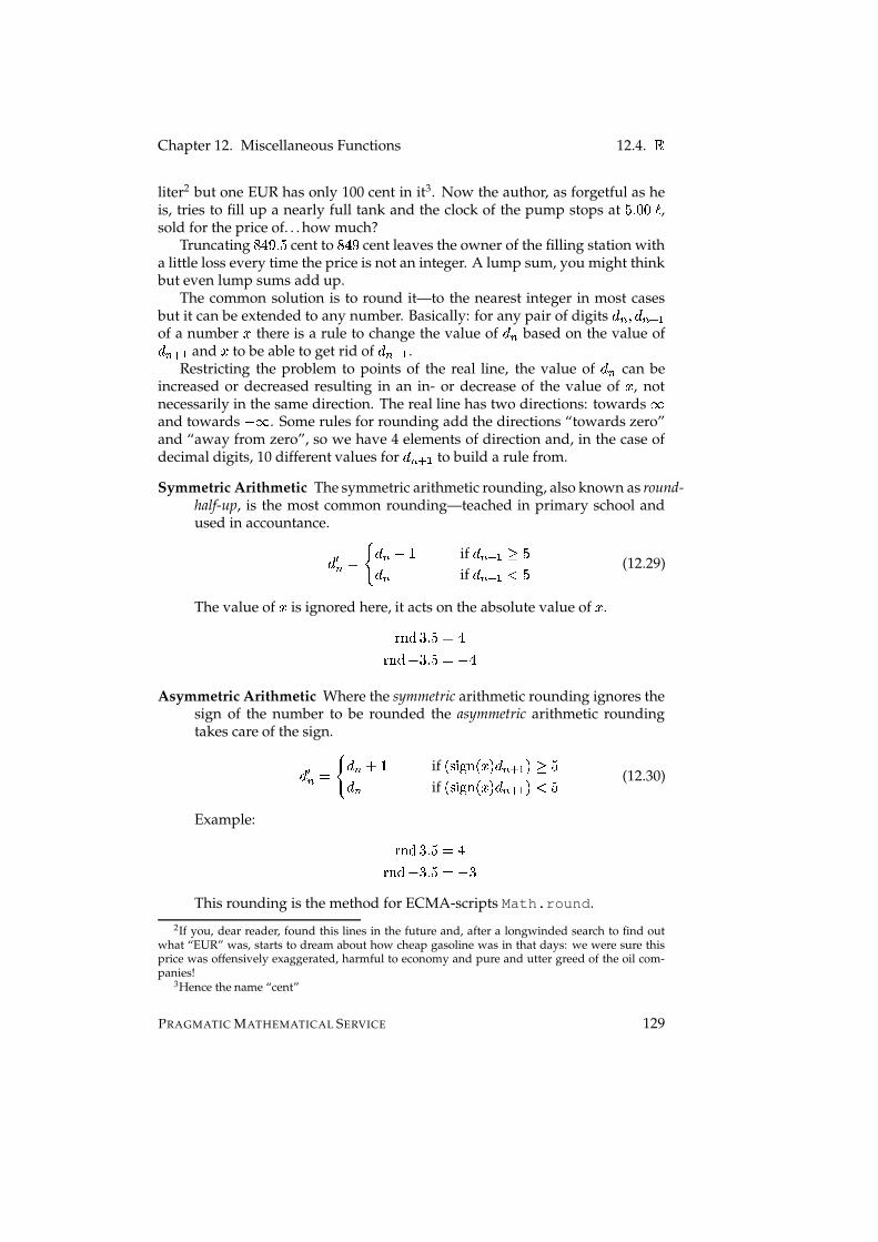
Chapter 12. Miscellaneous Functions 12.4. [liter2 but one EUR has only 100 cent in it3. Now the author, as forgetful as heis, tries to fill up a nearly full tank and the clock of the pump stops at ó � �!�dº ,sold for the price of. . . how much?
Truncating õ � � � ó cent to õ � � cent leaves the owner of the filling station witha little loss every time the price is not an integer. A lump sum, you might thinkbut even lump sums add up.
The common solution is to round it—to the nearest integer in most casesbut it can be extended to any number. Basically: for any pair of digits j C : j C
� "of a number A there is a rule to change the value of j C based on the value ofj C� " and A to be able to get rid of j C
� " .Restricting the problem to points of the real line, the value of j C can be
increased or decreased resulting in an in- or decrease of the value of A , notnecessarily in the same direction. The real line has two directions: towards gand towards w g . Some rules for rounding add the directions “towards zero”and “away from zero”, so we have 4 elements of direction and, in the case ofdecimal digits, 10 different values for j C
� " to build a rule from.
Symmetric Arithmetic The symmetric arithmetic rounding, also known as round-half-up, is the most common rounding—teached in primary school andused in accountance.
j âC I _ j C rL) if j C� " ¾ ój C if j C� " Ôó (12.29)
The value of A is ignored here, it acts on the absolute value of A .W� a � � ó6I �W� a w�� � ó6Ièw �Asymmetric Arithmetic Where the symmetric arithmetic rounding ignores the
sign of the number to be rounded the asymmetric arithmetic roundingtakes care of the sign.
j âC I _ j C rL) if �q'43Í^! ���A�� j C� " � ¾ ój C if �q'43Í^! ���A�� j C� " �8 Ôó (12.30)
Example: W� a � � ó6I �W� a w�� � ó6Ièw��This rounding is the method for ECMA-scripts Math.round.
2If you, dear reader, found this lines in the future and, after a longwinded search to find outwhat “EUR” was, starts to dream about how cheap gasoline was in that days: we were sure thisprice was offensively exaggerated, harmful to economy and pure and utter greed of the oil com-panies!
3Hence the name “cent”
PRAGMATIC MATHEMATICAL SERVICE 129
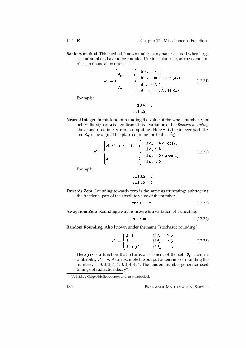
12.4. [ Chapter 12. Miscellaneous Functions
Bankers method This method, known under many names is used when largesets of numbers have to be rounded like in statistics or, as the name im-plies, in financial institutes.
j âC I ¹ºººº» ºººº¼ jC~r¶) _ if j C
� " ¾�ìif j C
� " I«óL1 ã»��ã� å� j C �j C _ if j C� " � �
if j C� " I«óL1Õ& a,a � j C �
(12.31)
Example: W� a � � ó6I¶�W� a � � ó6I«óNearest Integer In this kind of rounding the value of the whole number A , or
better: the sign of A is significant. It is a variation of the Bankers Roundingabove and used in electronic computing. Here A â is the integer part of Aand j C is the digit at the place counting the tenths ( "" ? ).
A â I ¹ºººº» ºººº¼'43Í^! ���A��<��à AÈà³rL)´� _ if j C I«óÌ1~& a,a ��A��if j C (ÔóA â _ if j C�I«óÌ1Qãã�$ã� ���A��if j C Ôó
(12.32)
Example: W� a � � ó6I �W� a � � ó6I �Towards Zero Rounding towards zero is the same as truncating: subtracting
the fractional part of the absolute value of the numberW� a AOI Y A([ (12.33)
Away from Zero Rounding away from zero is a variation of truncating.W� a AOIÆÅ A[Ç (12.34)
Random Rounding Also known under the name “stochastic rounding”.
j âC I ¹º» º¼ j C rL) if j C� " (Lój C if j C� " Lój C~r æ �z� if j C� " I ó (12.35)
Here æ �q� is a function that returns an element of the set k³��:�) l with aprobability
q I "$ . As an example the out put of ten runs of rounding thenumber � � ó : 3, 3, 3, 4, 4, 3, 3, 4, 4, 4. The random number generator usedtimings of radiactive decay4.
4A brick, a Geiger-Muller-counter and an atomic clock
130 PRAGMATIC MATHEMATICAL SERVICE

Chapter 12. Miscellaneous Functions 12.5. \12.4.2 Lucas Numbers
The Lucas numbers ([66]) are the same as the Fibonacci numbers with the ex-ception that the sequence starts with
/instead of � .
12.5 È12.5.1 Discrete Fourier Transformation
12.6 Leftovers fitting nowhere else
PRAGMATIC MATHEMATICAL SERVICE 131

12.6. Leftovers fitting nowhere else Chapter 12. Miscellaneous Functions
132 PRAGMATIC MATHEMATICAL SERVICE
Glossary
Affinely Extended Real Numbers It is the set [vMGk(w g¶:_règ l , a 2-point com-pactification of the real line. The common notation seems to be ��[@� . Thisset is not a field: for example règLr��4w gn� and w gLr��Þrègn� are not defined,so the inverse axiom of the field axiom does not hold here.
Blancmange Recipe by Paul Bocuse in [13]
250 g almonds, peeled2 bitter almonds
2/5 º fresh cream100 g sugar
1/2 tbl vanilla sugar7–8 leaves gelatine
1/10 º thick cream (creme fraıche)some extra sugar
Soak the almonds5 for at least 30 minutes in cold water, let them drippoff and pound them in a mortar until it is a fine paste. Add some dripsof water after the first minutes of pounding and later the cream in smallquantities6. Put the paste in a clean cloth and wring it out over a bowl.Solve the sugar, the vanilla sugar in that almond milk. Warm a smallquantity of that milk up to solve the gelatine in it. Add that mix to therest of the almond milk, let it cool off until the gelatine starts to set. Whipthe rest of the cream7 together with a bit of sugar and add. Fill into amold or dish, cool of in the refrigerator (at least 2 hours), unmold andserve.
Blancmange Function The Blancmange-function is a continuous function butnowhere differentiable. It is also called the “Takagi fractal curve” by [110]
5if they are not peeled: cook about five minutes, quench and press them between thumb andforefinger to slip the peel of. It is quite a mess, the author suggests to buy peeled almonds, theyare not very expensive.
6Yes, the whole process might last about 15–20 minutes!7 It is not in the recipe which of the two sorts of cream is meant to be whipped, but creme fraıche
is nearly impossible to whip
133
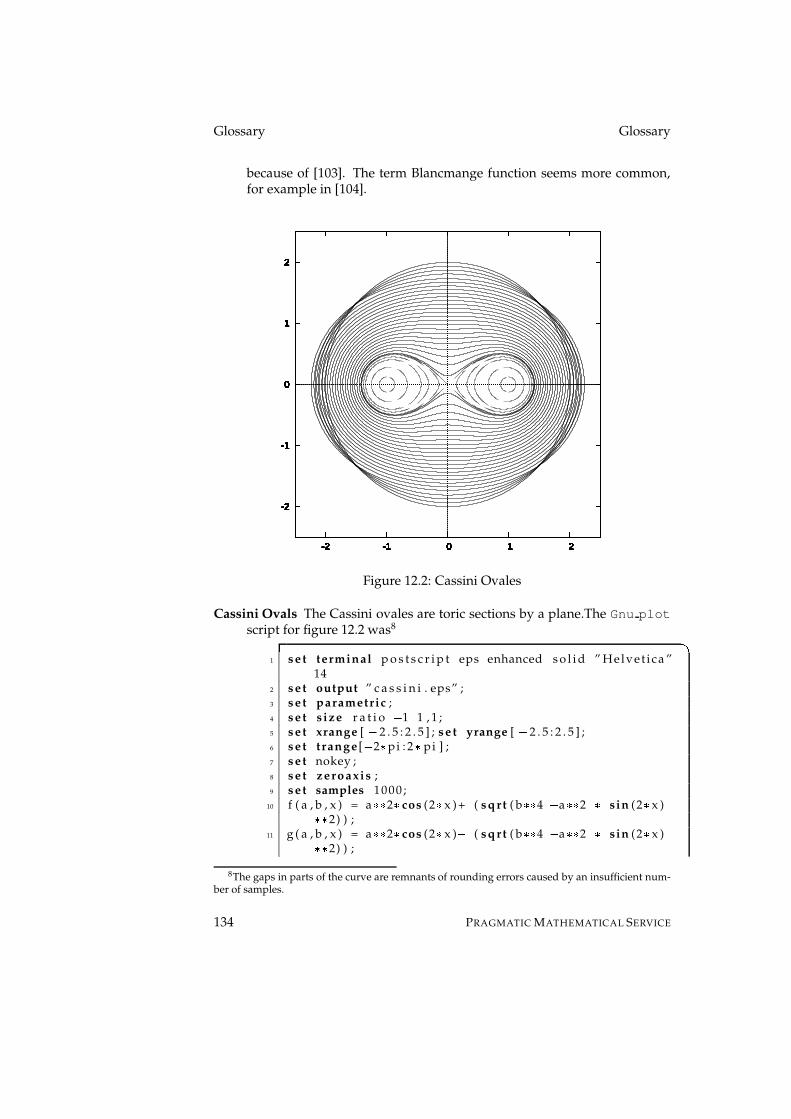
Glossary Glossary
because of [103]. The term Blancmange function seems more common,for example in [104].
-2
-1
0
1
2
-2 -1 0 1 2
-2
-1
0
1
2
-2 -1 0 1 2
-2
-1
0
1
2
-2 -1 0 1 2
-2
-1
0
1
2
-2 -1 0 1 2
-2
-1
0
1
2
-2 -1 0 1 2
-2
-1
0
1
2
-2 -1 0 1 2
-2
-1
0
1
2
-2 -1 0 1 2
-2
-1
0
1
2
-2 -1 0 1 2
-2
-1
0
1
2
-2 -1 0 1 2
-2
-1
0
1
2
-2 -1 0 1 2
-2
-1
0
1
2
-2 -1 0 1 2
-2
-1
0
1
2
-2 -1 0 1 2
-2
-1
0
1
2
-2 -1 0 1 2
-2
-1
0
1
2
-2 -1 0 1 2
-2
-1
0
1
2
-2 -1 0 1 2
-2
-1
0
1
2
-2 -1 0 1 2
-2
-1
0
1
2
-2 -1 0 1 2
-2
-1
0
1
2
-2 -1 0 1 2
-2
-1
0
1
2
-2 -1 0 1 2
-2
-1
0
1
2
-2 -1 0 1 2
-2
-1
0
1
2
-2 -1 0 1 2
-2
-1
0
1
2
-2 -1 0 1 2
-2
-1
0
1
2
-2 -1 0 1 2
-2
-1
0
1
2
-2 -1 0 1 2
-2
-1
0
1
2
-2 -1 0 1 2
-2
-1
0
1
2
-2 -1 0 1 2
-2
-1
0
1
2
-2 -1 0 1 2
-2
-1
0
1
2
-2 -1 0 1 2
-2
-1
0
1
2
-2 -1 0 1 2
-2
-1
0
1
2
-2 -1 0 1 2
-2
-1
0
1
2
-2 -1 0 1 2
-2
-1
0
1
2
-2 -1 0 1 2
-2
-1
0
1
2
-2 -1 0 1 2
-2
-1
0
1
2
-2 -1 0 1 2
-2
-1
0
1
2
-2 -1 0 1 2
-2
-1
0
1
2
-2 -1 0 1 2
Figure 12.2: Cassini Ovales
Cassini Ovals The Cassini ovales are toric sections by a plane.The Gnu plotscript for figure 12.2 was8 �
1 s e t terminal p o s t s c r i p t eps enhanced s o l i d ” Helvet i ca ”14
2 s e t output ” c a s s i n i . eps” ;3 s e t parametric ;4 s e t s ize r a t i o � 1 1 , 1 ;5 s e t xrange [ � 2 . 5 : 2 . 5 ] ; s e t yrange [ � 2 . 5 : 2 . 5 ] ;6 s e t trange [ � 2 � pi : 2 � pi ] ;7 s e t nokey ;8 s e t zeroaxis ;9 s e t samples 1000 ;
10 f ( a , b , x ) = a ��� 2 � cos (2 � x )+ ( sqr t ( b �(� 4 � a �(� 2 � sin (2 � x )�7� 2) ) ;11 g ( a , b , x ) = a ��� 2 � cos (2 � x ) � ( sqr t ( b �(� 4 � a �(� 2 � sin (2 � x )�7� 2) ) ;
8The gaps in parts of the curve are remnants of rounding errors caused by an insufficient num-ber of samples.
134 PRAGMATIC MATHEMATICAL SERVICE
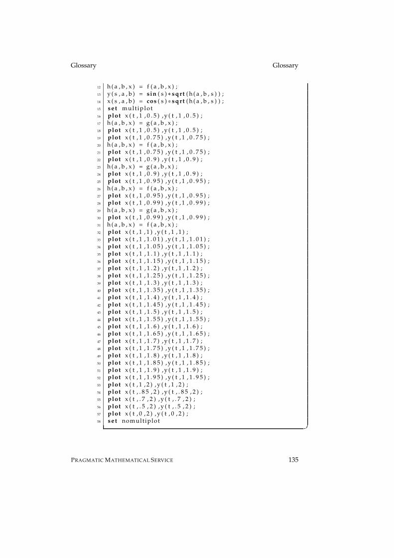
Glossary Glossary
12 h ( a , b , x ) = f ( a , b , x ) ;13 y ( s , a , b ) = sin ( s ) � sqr t ( h ( a , b , s ) ) ;14 x ( s , a , b ) = cos ( s ) � sqr t ( h ( a , b , s ) ) ;15 s e t mult ip lo t16 plot x ( t , 1 , 0 . 5 ) , y ( t , 1 , 0 . 5 ) ;17 h ( a , b , x ) = g ( a , b , x ) ;18 plot x ( t , 1 , 0 . 5 ) , y ( t , 1 , 0 . 5 ) ;19 plot x ( t , 1 , 0 . 7 5 ) , y ( t , 1 , 0 . 7 5 ) ;20 h ( a , b , x ) = f ( a , b , x ) ;21 plot x ( t , 1 , 0 . 7 5 ) , y ( t , 1 , 0 . 7 5 ) ;22 plot x ( t , 1 , 0 . 9 ) , y ( t , 1 , 0 . 9 ) ;23 h ( a , b , x ) = g ( a , b , x ) ;24 plot x ( t , 1 , 0 . 9 ) , y ( t , 1 , 0 . 9 ) ;25 plot x ( t , 1 , 0 . 9 5 ) , y ( t , 1 , 0 . 9 5 ) ;26 h ( a , b , x ) = f ( a , b , x ) ;27 plot x ( t , 1 , 0 . 9 5 ) , y ( t , 1 , 0 . 9 5 ) ;28 plot x ( t , 1 , 0 . 9 9 ) , y ( t , 1 , 0 . 9 9 ) ;29 h ( a , b , x ) = g ( a , b , x ) ;30 plot x ( t , 1 , 0 . 9 9 ) , y ( t , 1 , 0 . 9 9 ) ;31 h ( a , b , x ) = f ( a , b , x ) ;32 plot x ( t , 1 , 1 ) , y ( t , 1 , 1 ) ;33 plot x ( t , 1 , 1 . 0 1 ) , y ( t , 1 , 1 . 0 1 ) ;34 plot x ( t , 1 , 1 . 0 5 ) , y ( t , 1 , 1 . 0 5 ) ;35 plot x ( t , 1 , 1 . 1 ) , y ( t , 1 , 1 . 1 ) ;36 plot x ( t , 1 , 1 . 1 5 ) , y ( t , 1 , 1 . 1 5 ) ;37 plot x ( t , 1 , 1 . 2 ) , y ( t , 1 , 1 . 2 ) ;38 plot x ( t , 1 , 1 . 2 5 ) , y ( t , 1 , 1 . 2 5 ) ;39 plot x ( t , 1 , 1 . 3 ) , y ( t , 1 , 1 . 3 ) ;40 plot x ( t , 1 , 1 . 3 5 ) , y ( t , 1 , 1 . 3 5 ) ;41 plot x ( t , 1 , 1 . 4 ) , y ( t , 1 , 1 . 4 ) ;42 plot x ( t , 1 , 1 . 4 5 ) , y ( t , 1 , 1 . 4 5 ) ;43 plot x ( t , 1 , 1 . 5 ) , y ( t , 1 , 1 . 5 ) ;44 plot x ( t , 1 , 1 . 5 5 ) , y ( t , 1 , 1 . 5 5 ) ;45 plot x ( t , 1 , 1 . 6 ) , y ( t , 1 , 1 . 6 ) ;46 plot x ( t , 1 , 1 . 6 5 ) , y ( t , 1 , 1 . 6 5 ) ;47 plot x ( t , 1 , 1 . 7 ) , y ( t , 1 , 1 . 7 ) ;48 plot x ( t , 1 , 1 . 7 5 ) , y ( t , 1 , 1 . 7 5 ) ;49 plot x ( t , 1 , 1 . 8 ) , y ( t , 1 , 1 . 8 ) ;50 plot x ( t , 1 , 1 . 8 5 ) , y ( t , 1 , 1 . 8 5 ) ;51 plot x ( t , 1 , 1 . 9 ) , y ( t , 1 , 1 . 9 ) ;52 plot x ( t , 1 , 1 . 9 5 ) , y ( t , 1 , 1 . 9 5 ) ;53 plot x ( t , 1 , 2 ) , y ( t , 1 , 2 ) ;54 plot x ( t , . 8 5 , 2 ) , y ( t , . 8 5 , 2 ) ;55 plot x ( t , . 7 , 2 ) , y ( t , . 7 , 2 ) ;56 plot x ( t , . 5 , 2 ) , y ( t , . 5 , 2 ) ;57 plot x ( t , 0 , 2 ) , y ( t , 0 , 2 ) ;58 s e t nomult iplot �
PRAGMATIC MATHEMATICAL SERVICE 135
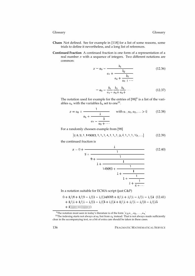
Glossary Glossary
Chaos Not defined. See for example in [118] for a list of some reasons, sometrials to define it nevertheless, and a long list of references.
Continued Fraction A continued fraction is one form of a representation of areal number A with a sequence of integers. Two different notations arecommon: AVIL9�?Sr ; "9 " r ; $9 $ r ; ê9 ê rLë�ë�ë
(12.36)
IL9�?Sr ; "9 " r ; $9 $ r ; ê9 ê r ë�ë�ë (12.37)
The notation used for example for the entries of [98]9 is a list of the vari-ables 9�C with the variables ;<C set to one10.A¸I¶9 ? r )9 " r )9 $ r )9 ê rLë�ë�ë
with 9 " :�9 $ :�9 ê : ����� (Ô� (12.38)
For a randomly choosen example from [98]� �(w�õ�:���:�)!:�) � �!�!õ(�7:�)!:�)(:�)�: � :<)(:�)�:�)!:��|: � :<)!:�)�:�)(:�)�ó7: ����� � (12.39)
the continued fraction isAOIL��r )õ�r )��r ))xr )) � �!�!õ(�±r ))xr ))xr ))}r )� rLë�ë�ë
(12.40)
In a notation suitable for ECMA-script (just C&P)��r¶)f}7��õ�rL)�}|�q��rL)�}|�°)}r¶)f}7�°) � �!�(õ!�Sr¶)f}7�°)}r¶)f}|�4)}rL)�}|�°)xr¶)f}7� � (12.41)r¶)f}7�°)}rL)�}|�4)xrL)�}|�°)}r¶)f}7����rL)�}|� � r¶)f}7�°)xr¶)f}7�°)}rL)�}|�4){r¶)f}7�°)´ór¶)³���4�4���4���4�4���4���4�4���4���9The notation most seen in today’s literature is of the form É Ê�Ë©Ì�Ê ë ��Ê ï �=¦ ¦ ¦���Ê ©9Í10The indexing starts not always at Ê Ë but from Ê ë instead. That is not always made sufficiently
clear in the accompanying text, so a bit of extra care should be taken in these cases.
136 PRAGMATIC MATHEMATICAL SERVICE

Glossary Glossary
Running gives � � ) / � � ó ì í�õ!�7)³�7)�)() , which is Champernowns constant to 13digits precision. The real precision of the continued fraction 12.41 is 185digits, the twenty digits 9 " < ? – 9 $ ?�? are �(ó!� ì ��í�� ³ �(�!�7)³� / �(��� � �(óChampernowns constant had been choosen as an example because it isextremely easy to check the correctness of the result and because the con-tinued fraction expansion has a weird pattern11 and is very hard to ob-tain.
Getting a continued fraction expansion is quite simple, at least in theory:
Example 12.6.1. Some warm-up: we are looking for the continued frac-tion expansion of
. /. The rules are simple:� ? I � (12.42)9�C�I Y � CS[ (12.43)� C � " I )� CÇwy9�C (12.44)
9 ? IÏÎ . /�Ð IN) (12.45)� " I ). / w�) (12.46)I . / r¶)/ w�)I . / r¶)9 " I Î . / rL) Ð I / (12.47)� $ I ). / r¶)²w / (12.48)I ). / w�)I . / r¶)/ w�)I . / r¶)9 $ I Î . / rL) Ð I / (12.49)
We can stop here because it is obvious that the partial quotients are al-ways
/. So, with the overline marking the periodical sequence, the con-
tinued fraction expansion of. /
is ��),w / � .11The next partial quotient Ê ënÑ is Ò�¦ §�¨�§-Ò�Ó�ß ¥ ënÔ�Õ
PRAGMATIC MATHEMATICAL SERVICE 137

Glossary Glossary
Computing the expansion with ten partial quotients (again fit for a simpleC&P) )xr¶)f}|� / rL)�}|� / r¶)f}7� / r¶)f}|� / rL)�}|� / r¶)f}7� / r)f}7� / r¶)f}|� / rL)�}|� / r¶)f}7� / �4�4���4���4�4���4� (12.50)I õ7)!)³�ó(í � )7 ) � � ) � / )³�(ó!ó7) (12.51). / 7 ) � � ) � / )³�(ó ì / (12.52)
Ten partial quotients give seven decimal digits precision, not a very highconverging speed but at least easy to compute.
The error is approximately the multiplicative inverse of the square of thelast denominator. In this case)ó(í � ) $ 7 � � �!� � Te)�� ® ? < (12.53)
In the case of Champernowns constant)� �(�!�(ó!�!�(�!�!�(�!� $ 7 � � ) ì � Te)�� ® $ À (12.54)
which is a bit off. Including partial quotient 9 " < gives an approxximationof ) � �!õ(�ÁTV)³� ® ê �;� , which even more off. The arithmetic mean of the expo-nents is )�õ(� � ó which seems more passable in relation to the real precisionof 185 decimal digits.
Dirichlet & -function The Dirichlet & -function is defined by the sum&}��A��}I î�C � ? �°w6)´� C � / �µrL)´� ®�Ò (12.55)
Equivalent equations include&}��A��xI / ®öÒ ~ ð*w6)!:�Aå: )/ ñ (12.56)I )� Ò * � ð A�: )� ñ w¬� ð A�: �� ñ + (12.57)
Where �7��Aå:�9�� is Hurwitz’ � -function and~ �qÆ�:�'(:�9|� is the Lerch transcen-
dent.
Extending the & -function to the complex plane can be done by&x�°)�wyÆ��@I ð /� ñD '435 ð )/ � Æ�=}�qÆ�� &}��Æ�� ñ (12.58)
where =}�q�� is the = -function.
138 PRAGMATIC MATHEMATICAL SERVICE

Glossary Glossary
Field A field is unsuprisingly defined by its axioms
Name Addition MultiplicationCommutativity 9,rt;²I¶;@rv9 9|;SI ;�9
Associativity �q9srt;<�årnu�IL9sr �z;2rnu�� ��9|;<�4u²I«9ö�q;�u��Distributivity 9��z;{rvu��{IL9|;@rv9�u �q9,rt;<�4u²I¶9�u}rn;�u
Identity 96rv�~I«9ËI¶��rv9 9~ë!)�I«9ËIè)²ë�9Inverse 9sr«�°w�9|�{I«�ÕIè�4w�9���rv9 9 "¡ IN)ÁI "¡ 9 with 9 HIL�
Iverson Bracket The Iverson bracket ([48]) is a notation for a numerical equiv-alence of a Boolean result. Given a mathematical statement 1 , then thedefinition and notation is� 1d�*I _ � if 1 is false) if 1 is true
(12.59)
The notation with the brackets � A,� is sometimes used for the floor functionand for rounding to the nearest integer, too. The former is rarely seen,the notation Y A([ is probably the most common in the time of this writing.The latter used should be made clear by the accompanying text or, if thatis not possible, with the named operator 735 ��³��A�� , which seems to be themost common abbreviation for that kind of rounding.
-0.6
-0.4
-0.2
0
0.2
0.4
0.6
-1 -0.5 0 0.5 1
Figure 12.3: Lemniscate
Lemniskate The lemniscate or Bernoulli’s lemniscate12 is a special form of
12Bernoulli described that curve in [9]
PRAGMATIC MATHEMATICAL SERVICE 139
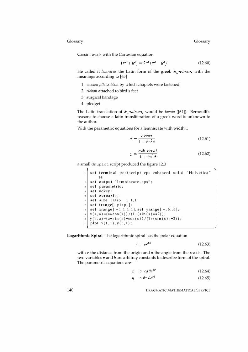
Glossary Glossary
Cassini ovals with the Cartesian equationu A $ r¬Ö $ w I / u $ u A $ weÖ $ w (12.60)
He called it lemnicus the Latin form of the greek � % å�×Ö] R m �f� with themeanings according to [65]
1. woolen fillet,ribbon by which chaplets were fastened
2. ribbon attached to bird’s feet3. surgical bandage4. pledget
The Latin translation of � % å�×Ö] R m �f� would be taenia ([64]). Bernoulli’sreasons to choose a latin transliteration of a greek word is unknown tothe author.
With the parametric equations for a lemniscate with width 9A¸I 9x%�&('æ�)xrv'�3� $ � (12.61)
Ö�I 9x'�3� %�|%<&�'æ�)xrn'435 $ � (12.62)
a small Gnuplot script produced the figure 12.3 �1 s e t terminal p o s t s c r i p t eps enhanced s o l i d ” Helvet i ca ”
142 s e t output ” lemnisca te . eps” ;3 s e t parametric ;4 s e t nokey ;5 s e t zeroaxis ;6 s e t s ize r a t i o � 1 1 ,17 s e t trange[ � pi : pi ] ;8 s e t xrange [ � 1 . 1 : 1 . 1 ] ; s e t yrange [ � . 6 : . 6 ] ;9 x ( s , a ) =( a � cos ( s ) ) /(1+( sin ( s ) �7� 2) ) ;
10 y ( s , a ) =( a � sin ( s ) � cos ( s ) ) /(1+( sin ( s ) �7� 2) ) ;11 plot x ( t , 1 ) , y ( t , 1 ) ; �
Logarithmic Spiral The logarithmic spiral has the polar equation* IL9�0 9 É (12.63)
with * the distance from the origin and Ñ the angle from the x-axis. Thetwo variables 9 and ; are arbitray constants to describe form of the spiral.The parametric equations are AOI¶9x%�&('|Ñ(0 9 É (12.64)Ö�I¶9x'�35 ²Ñ!0 9 É (12.65)
140 PRAGMATIC MATHEMATICAL SERVICE
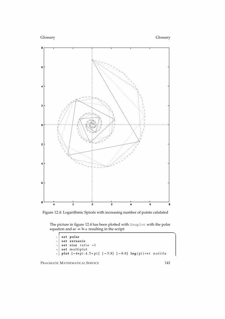
Glossary Glossary
8
6
4
2
0
2
4
6
8
4 2 0 2 4 6 8 8
6
4
2
0
2
4
6
8
4 2 0 2 4 6 8 8
6
4
2
0
2
4
6
8
4 2 0 2 4 6 8 8
6
4
2
0
2
4
6
8
4 2 0 2 4 6 8 8
6
4
2
0
2
4
6
8
4 2 0 2 4 6 8
Figure 12.4: Logarithmic Spirals with increasing number of points calulated
The picture in figure 12.4 has been plotted with Gnuplot with the polarequation and 9�0sI �� � resulting in the script: �
1 s e t polar2 s e t zeroaxis3 s e t s ize r a t i o � 14 s e t mult ip lo t5 plot [ � 4 � pi : 4 . 5 � pi ] [ � 5:8] [ � 8:8] log ( pi ) �!� t n o t i t l e
PRAGMATIC MATHEMATICAL SERVICE 141
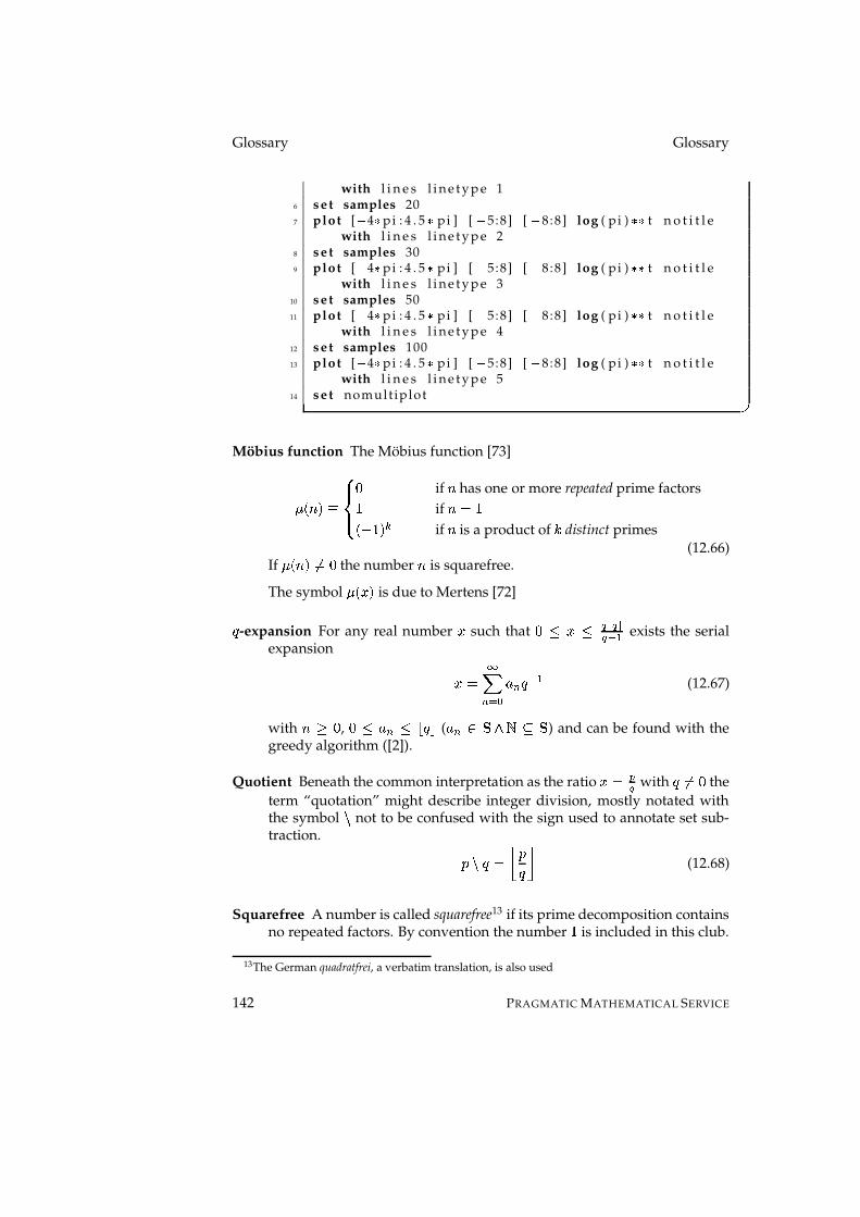
Glossary Glossary
with l i n e s l i n e t y p e 16 s e t samples 207 plot [ � 4 � pi : 4 . 5 � pi ] [ � 5:8] [ � 8:8] log ( pi ) �(� t n o t i t l e
with l i n e s l i n e t y p e 28 s e t samples 309 plot [ � 4 � pi : 4 . 5 � pi ] [ � 5:8] [ � 8:8] log ( pi ) �(� t n o t i t l e
with l i n e s l i n e t y p e 310 s e t samples 5011 plot [ � 4 � pi : 4 . 5 � pi ] [ � 5:8] [ � 8:8] log ( pi ) �(� t n o t i t l e
with l i n e s l i n e t y p e 412 s e t samples 10013 plot [ � 4 � pi : 4 . 5 � pi ] [ � 5:8] [ � 8:8] log ( pi ) �(� t n o t i t l e
with l i n e s l i n e t y p e 514 s e t nomult iplot �
Mobius function The Mobius function [73]
���å� Z ¹º» º¼� if � has one or more repeated prime factors) if �iIN)�°w6)´� ï if � is a product of ò distinct primes
(12.66)If ���å� HI«� the number � is squarefree.
The symbol ��A�� is due to Mertens [72]� -expansion For any real number A such that � �ÓA � L � L �L ® " exists the serialexpansion AVI î�C � ? 9�C � ® " (12.67)
with � ¾ � , �4�R9 C � Y � [ ( 9 C �]� 1ÇW / � ) and can be found with thegreedy algorithm ([2]).
Quotient Beneath the common interpretation as the ratio AOI K L with � HIL� theterm “quotation” might describe integer division, mostly notated withthe symbol Q not to be confused with the sign used to annotate set sub-traction. � Q � IÙØ � ��Ú (12.68)
Squarefree A number is called squarefree13 if its prime decomposition containsno repeated factors. By convention the number ) is included in this club.
13The German quadratfrei, a verbatim translation, is also used
142 PRAGMATIC MATHEMATICAL SERVICE

Glossary Glossary� factors squarefree1 1 yes2 2 yes3 3 yes4
/ ë / no5 5 yes6
/ � yes7 7 yes8
/ ë / ë / no9 �,ë�� no
10/ ë³ó yes
The asymptotic density e of such numbers �e6I )��� / � for �G�VW (12.69)
Here, as elsewhere, �����å� is Riemann’s � -function.
The equivalent for the integers on the complex plane, the Gaussian inte-gers, e,I ì� $ � (12.70)� is Catalan’s constant
Stirling Number of the Second Kind A Stirling number of the second kind1²�X%e:�ò7� describes the number of collections Û � of same-sized non-emptysubsets Ü C of a power set
q �q1}� . More formaly:���N(Ô� (12.71)Û � /ok q �z1{��QÝM l (12.72)ÜxC2/OÛ � (12.73)Û � I k$k§Ü{?(:ÂÜ " : ����� :ÞÜ}C l � ��ÜxC�Io��Ü}C� " 1aÜ}C HITM l (12.74)% I���� (12.75)ò�I���Ü}C (12.76)1²�X%e:�ò7�{I��)k§Û ? :ÞÛ " : ����� :-Û � l (12.77)
Some examples with the set �©I k / :���: � l :q �z1{�@I k'MÇ:�k / l : k³� l :�k � l : k / :�� l : k / : � l : k³�|: � l : k / :��|: � lxl (12.78)1²�q�7:�)´�@Io�)k$k�k / l :�k´� l :�k � l$l�l Iè) (12.79)1²�q�7: / �@Io�)k$k / :�� l : k / : � l :�k´�7: � lxl I¶� (12.80)1²�q�7:����@Io�)k$k / :��7: � l$l IÍ) (12.81)
PRAGMATIC MATHEMATICAL SERVICE 143
Glossary Glossary
Thue-Morse Sequence The Thue-Morse sequence can can be easily generatedwith the substitution map � à �7) (12.82)) àc)�� (12.83)
Interpreted as the concatenation of binary digits gives the Thue-Morseconstant.
Wronskian The Wronskian, or Wronski-determinant, is defined for a set offunctions differentiable over an interval � by÷ � æ!" : æ $ : ����� : æ C �<��A�� Z ���������
æ " æ $ ë�ë�ë æ Cæ â" æ â$ ë�ë�ë æ âC......
. . ....æ C ® "4¯" æ C ® "4¯$ ë�ë�ë æ C ® "4¯C ���������
(12.84)
If the Wronskian is non-zero somewhere on the interval � the functionsare said to be linearly independent on the interval.
Example:Given the interval [ and the three functions æ " ��Aö�}Iè) , æ $ I¶A and æ ê ILA êwhich are luckily defined for every A � [ and are easily differentiablewithout the help of a CAS14. The Wronskian is in that case÷ � æ!" : æ $ : æ ê ����Aö� Z ������
) A A ê� )Ã��A $� � ì A ������(12.85)
The determinant of a �sTÇ� square matrix can be calculated without muchheadache by strictly following Sarrus’ rule��9 "�" 9 $�$ 9 ê�ê � (12.86)rÇ��9 " $ 9 $ ê 9 ê " �rÇ��9 " ê 9 $ " 9 ê $ �w6��9 " ê 9 $�$ 9 ê " �w6��9 " $ 9 $ " 9 ê�ê �w6��9 "�" 9 $ ê 9 ê $ �Filling the blanks and calculating15 the determinant comes out as
ì A whichis evidently non-zero on the given interval, the real line, so the functionsare linearly independent.
14Just in case: the derivative of a constant is 0(zero), the derivative of a power is o�Ó © Ø � o�Ó © Õ ë(with o constant, the coeficient) which means for an exponent of 1(one): Ó ë ØFßàßJÓ éÉë Õ ëåì ØGßàßJÓ Ë Øß½ß�ß�ØGß
15Which has been left as an exercise to the reader, of course.
144 PRAGMATIC MATHEMATICAL SERVICE

Glossary Glossary
For another example consider the three functions æ�" ��A��6I ) , æ $ ��A��6IRA $and æ ê ��A��}I«��r / A $ over the interval [ . The Wronskian is÷ � æ " : æ $ : æ ê �<��A�� Z ������
) A $ ��r / A $� / A � A� / � ������IL� (12.87)
This result is a hint, that these functions might be linearly dependent,but it is not mandatory! We can see by further inspection that æ ê ��A���I� æ " ��A��2r / æ $ ��Aö� . That rule has it’s continuation in the relation of the col-umn vectors u ê I �(u " r / u $ so these three functions are in fact linearlydependent.
It is not sufficient to assume that the functions are linearly independentfrom the value of the Wronski-determinant alone if that determinant iszero everywhere. A counter-example is easily constructed with the twofunctions æ!" ��A��xILA $ à A2à and æ $ ��Aö�}IÔA ê over the interval �°w6)(:�)´� �i[ 16 . æ("is differentiable at A¸I«� and
æ!" ��A��}I`_ w���A $ if Aá Ô���A $ if A ¾ � (12.88)
The Wronskians are then÷ � æ " : æ $ �<��A�� Z ¹ººººº» ººººº¼�����A ê A ê��A $ ��A $ ����� I«� if A ¾ ������w²A ê A êw���A $ ��A $ ����� I¶� if Aá t� (12.89)
So for all A-�«�°w6)(:�)´� the Wronski-determinant is
÷ � æ " : æ $ �ÁI � . Never-theless it is obvious that these two functions are linearly independant on�°w6)!:�)³� , moreso on any interval �IN��9�:�;�� with k³� l �{ .
16Note that contrary to most textbooks the derivative of the function áSÇÍÓ,ÊåØAâ Ó[â does not exist.Only if it is restricted to the real line derivatives exist for all points except 0
PRAGMATIC MATHEMATICAL SERVICE 145

Glossary Glossary
146 PRAGMATIC MATHEMATICAL SERVICE

Bibliography
Qualem commendes, etiam atque etiam aspice, ne moxincutiant aliena tibi peccata pudorem.[QUINTUS HORATIUS FLACCUS,“Epistulae”, I,18,76]
Copy from one, it’s plagiarism; copy from two, it’s research.[WILSON MIZNER (1876–1933)]
[1] Milton Abramowitz and Irene A. Stegun, editors.Handbook of Mathematical Functions.Dover, New York, � th edition, 1965.
[2] J.-P. Allouche and M. Cosnard.The Komornik-Loreti constant is transcendental.Amer. Math. Monthly, 107:448–449, 2000.
[3] H. Alzer.Some gamma function inequalities.Math. Comput., 60:337–346, 1993.
[4] T. C.; Anderson, P. G.; Brown and P. J.-S. Shiue.A simple proof of a remarkable continued fraction identity.Proc. Amer. Math. Soc., 123:2005–1009, 1995.
[5] R. Andre-Jennin.Irrationalite de la somme des inverses de certaines suites recurrentes.C. R. Acad. Sci. Paris Ser. I Math., 308:539–541, 1989.
[6] E. Artin.Collected Papers.Springer–Verlag, New York, 1965.
[7] D. H. Bailey, J. M. Borwein, and R. E. Crandall.On the Khintchine constant.Math. Comput, 66:417–431, 1907.
[8] R. J. Baxter.Hard hexagons: Exact solution.J. Physics, 13:1023–1030, 1980.
147

Bibliography Bibliography
[9] J. Bernoulli.Constructio facilis Curvae accessus aequabilis a puncto dato per Rectifi-
cationem Curvae Algebraicae.Acta Eruditorum, pages 394–399, 1694.
[10] S. N. Bernstein.Sur la meilleure approximation de à A2à par les polynomes de degres tres
eleves.Bull. Acad. Sci., Cl. sci. math. nat 2:181–190, 1938.
[11] S. N. Bernstein.Sur la meilleure approximation de à A2à par les polynomes de degres
donnes.Acta Math., 37:1–57, 1957.
[12] K. Biggs.A precise computation of the Gauss-Kuzmin-Wirsing constant.2003.
[13] Paul Bocuse.La Cuisine de Marche.Flammarion, Paris, 1998.
[14] J. Borwein and D. Bailey.Mathematics by Experiment: Plausible Reasoning in the 21st Century.A. K. Peters, Wellesley, MA, 2003.
[15] J.; Borwein, D.; Bailey, and R. Girgensohn.Experimentation in Mathematics: Computational Paths to Discovery.A. K. Peters, Wellesley, MA, 2004.
[16] K. Briggs.A Precise Calulation of the Feigenbaum Constants.Math. Comput., 57:435–439, 1991.
[17] D Broadhurst.Feigenbaum constants to 1018 decimal places.1999.
[18] D. S.; Bullen, P.S.;Mitrinovic and P.M. Vasic.Means and their Inequalities.Reidel, Dordrecht, Netherlands, 1988.
[19] E. Cahen.Note sur un developpement des quantites numeriques, qui presente
quelque analogie avec celui des fractions continues.Nouv. Ann. Math., 10:508–514, 1891.
[20] Amos J. Carpenter and Richard S. Varga.Some numerical results on best uniform polynomial approximation of A ¼
on � �(w�) � . methods of approximation theory in complex analysis andmathematical physics.
1993.
148 PRAGMATIC MATHEMATICAL SERVICE
Bibliography Bibliography
http://www.math.kent.edu/˜varga/pub/paper_189.pdf, vis-ited at Mon Jun 23 12:14:15 CEST 2008. This article was reissued laterin ”Lecture Notes in Mathematics” (Springer Verlag),1993, pp. 192–222.
[21] E Catalan.Recherches sur la constant G, et sur les integrales euleriennes.Memoires de l’Academie imperiale des sciences de Saint-Petersbourg, Ser. 7,
1833.
[22] J. H. Conway.The weird and wonderful chemistry of audioactive decay.Open Problems in Communications and Computation, pages 173–188, 1987.
[23] J. H. Conway and R. K. Guy.The look and say sequence.The Book of Numbers, pages 208–209, 1996.
[24] M. Embree and L. N Trefethen.Growth and Decay of Random Fibonacci Sequences.Proceedings of the Royal Society, A 455(July):2471–2485, 1999.
[25] Die Fachredaktionen des Bibliographischen Instituts, editor.MEYERS Großer Rechenduden, volume 1.Bibliographisches Institut AG, Mannheim, Germany, 1964.
[26] M. J. Feigenbaum.The universal metric properties of nonlinear transformations.J. Stat. Phys., 21:669–706, 1979.
[27] S. R. Finch.Mathematical Constants.Cambridge University Press, Cambridge, England, 2003.
[28] P. Flajolet and I. Vardi.Zeta function expansions of classical constants.1996.
[29] A. Fransen.Accurate determination of the inverse gamma integral.BIT, 19:137–138, 1979.
[30] A. Fransen.Addendum and corrigendum to ‘high-precision values of the gamma
function and of some related coefficients’.Math. Comp., 37:233–235, 1981.
[31] A. Fransen and S. Wrigge.High-precision values of the gamma function and of some related coeffi-
cients.Math. Comp., 34:553–566, 1980.
[32] Alexandre Froda.Sur l’irrationalite du nombre
/�z.
PRAGMATIC MATHEMATICAL SERVICE 149

Bibliography Bibliography
Atti Accad. Naz. Lincei Rend. Cl. Sci. Fis. Mat. Natur., 35:472–478, 1963.
[33] M. Gardner.Penrose Tiles and Trapdoor Ciphers. . . and the Return of Dr. Matrix, reissue ed.W. H. Freeman, New York, 1991.
[34] J. W. L. Glaisher.On a numerical continued product.Messenger Math., 6:71–76, 1877.
[35] J. W. L. Glaisher.On the product ) " / " � ê ë�ë�ë4� C .Messenger Math., 7:43–47, 1878.
[36] J. W. L. Glaisher.On the constant which occurs in the formula for ) " / " � ê ë�ë�ë4� C .Messenger Math., 24:1–16, 1894.
[37] J. Gleick.Choas.Penguin Books, London, 1987.
[38] S. W. Golomb.Random Permutations.Bull. Amer. Math. Soc., 70, 1954.
[39] A. A. Gonchar and E. A. Rakhmanov.Equilibrium distributions and degree of rational approximation of ana-
lytic functions.Math. USSR Sbornik, 62:305–348, 1980.
[40] Bill Gosper.The information in a typical continued fraction term. . . .Math–fun list, April � th, 1998.
[41] A. Grothendieck.Elements de geometrie algebrique (rediges avec la collaboration de Jean
Dieudonne), I.Le langage des schemas.Publications Mathematiques de l’IHES, 4:5–228, 1960.
[42] G. H. Halphen.Traite des Fonctions Elliptiques et de Leurs Application.Paris, 1886–1889.
[43] J. Havil.Gamma: Exploring Euler’s Constant.Princeton University Press, Princeton, NJ, 2003.
[44] L. Hoehn and I. Niven.Averages on the move.Math. Mag., 58:151–156, 1985.
[45] ISO/IEC.Information technology – Programming languages – C.
150 PRAGMATIC MATHEMATICAL SERVICE

Bibliography Bibliography
International Standard ISO/IEC 9899:1999, International Standards Or-ganization, 1999.
[46] ISO/IEC.Information technology – ECMA-Script language specification.International Standard ISO/IEC 16262:2002, International Standards Or-
ganization, 2002.
[47] ISO/IEC.Information technology – Z formal specification notation – Syntax, type
system and semantics.International Standard ISO/IEC 13568:2002, International Standards Or-
ganization, 2002.
[48] K. E. Iverson.A Programming Language.Wiley, New York, 1962.
[49] G. S. Joyce.Exact results for the activity and isothermal compressibility of the hard-
hexagon model.J. Physics A: Math. Gen., 21:L983–L988, 1988.
[50] J. F. Kenney and E. S. Keeping.Mathematics of Statistics, volume 1.Van Nostrand, Princeton, NJ, 3rd edition, 1962.
[51] A. Ya. Khinchine.Continued Fractions.Dover, New York, 1997.
[52] A. Khintchine.Metrische Kettenbruchprobleme.Compositio Math., 1:361–382, 1934.
[53] A. Khintchine.Metrische Kettenbruchprobleme.Compositio Math., 2:276–285, 1936.
[54] Kinkelin.Uber eine mit der Gammafunktion verwandte Transcendente und deren
Anwendung auf die Integralrechnung.J. reine angew. Math., 57:122–158, 1860.
[55] Donald E. Knuth.The Art of Computer Programming—Seminumerical Algorithms, volume 2.Addison-Wesley, Reading, MA, 3 edition, 1998.
[56] V. Komornik and P. Loreti.Unique developments in non-integer bases.Amer. Math. Monthly, 105:636–639, 1998.
[57] Gabriel Lame.
PRAGMATIC MATHEMATICAL SERVICE 151
Bibliography Bibliography
Examen des differentes methodes employees pour resoudre les problemes degeometrie.
Vve. Courcier, Paris, 1818.
[58] E. Landau.Uber die Einteilung der positiven ganzen Zahlen in vier Klassen nach der
Mindeszahl der zu ihrer additiven Zusammensetzung erforderlichenQuadrate.
Arch. Math. Phys., 13:305–312, 1908.
[59] Francois le Lionnais.Les nombres remarquables.Hermann, France, 1983.
[60] D. H. Lehmer.A cotangent analogue of continued fractions.Duke Math. J., 4:323–340, 1938.
[61] D. H. Lehmer.Note on an absolute constant of khintchine.Amer. Math. Monthly, 46:148–152, 1938.
[62] T. Lengyel.On a recurrence involving stirling numbers.Europ. J. Comb, 5:313–321, 1984.
[63] P Levy.Sur le developpement en fraction continue d’un nombre choisi au
hasard.Compositio. Math., 3:286–303, 1936.
[64] H. G. Liddell and R. Scott.An Intermediate Greek-English Lexicon.Clarendon Press, Oxford, 1898.
[65] H. G. Liddell and R. Scott.A Greek-English Lexicon. revised and augmented throughout by. Sir Henry
Stuart Jones. with the assistance of. Roderick McKenzie.Clarendon Press, Oxford, 1940.
[66] F. E. Lucas.Theorie des fonctions numeriques simplement periodiques.Amer. J. of Math. pure and applied, 1:184–251,289–321, 1878.
[67] E. Madelung.without title.Phys. Zs., 19, 1918.
[68] F. Magata.Newtonian interpolation and primes.1998.
[69] A. P. Magnus.CFGT determination of Varga’s constant 1/9.
152 PRAGMATIC MATHEMATICAL SERVICE

Bibliography Bibliography
Inst. Preprint B-1348, 1986.
[70] A. P Magnus.On the use of the Caratheodory-fejer method for investigating ": and sim-
ilar constants.Nonlinear Numerical Methods and Rational Approximation (Wilrijk, 1987).,
pages 105–132, 1988.
[71] F. Mertens.without title.J. fur Math., 78:46–62, 1874.
[72] F. Mertens.Uber einige asymptotische Gesetze der Zahlentheorie.J. reine angew. Math., 77:46–62, 1874.
[73] A. F. Mobius.Uber eine besondere Art von Umkehrung der Reihen.J. reine angew. Math., 9:105–123, 1832.
[74] NASA.Glossary: Astronomical unit (AU).http://neo.jpl.nasa.gov/glossary/au.html, visited at Mon
Jul 21 23:57:51 CEST 2008.
[75] N. Nielsen.Theorie des Integrallogarithmus und Verwandter Transzendenten.Chelsea, New York, 1995.
[76] I. Niven.Averages of exponents in factoring integers.Proc. Amer. Math. Soc., 22:256–360, 1969.
[77] M. G. Norman and P. Moscato.The euclidean traveling salesman problem and a space-filling curve.Chaos Solitons Fractals, 6:389–397, 1995.
[78] G. H. Norton.On the asymptotic analysis of the Euclidean algorithm.J. Symb. Comput., 10:53–58, 1990.
[79] National Institute of Standards and Technology.Fundamental physical constants from NIST.http://physics.nist.gov/cuu/Constants/index.html vis-
ited at Wed Jul 23 01:51:26 CEST 2008, 2006.
[80] I. Palasti.On some random space filling problems.Publ. Math. Inst. Hung. Acad. Sci., 5:353–359, 1960.
[81] R. B. Paris.An asymptotic approximation connected with the golden number.Amer. Math. Monthly, 94:272–278, 1987.
PRAGMATIC MATHEMATICAL SERVICE 153
Bibliography Bibliography
[82] Petermann, Remy, and Vardi.Discrete Derivatives of Sequences.ADVAM: Advances in Applied Mathematics, 27, 2001.Full text at http://www.lix.polytechnique.fr/Labo/Ilan.
Vardi/discrete_derivatives.ps visited at Wed Jul 9 23:00:04CEST 2008.
[83] C. Pisot.La repartition modulo 1 et les nombres algebriques.Annali di Pisa, 7:205–248, 1938.
[84] A. Porges.A set of eight numbers.Amer. Math. Monthly, 52:379–382, 1945.
[85] J. W. Porter.On a theorem of Heilbronn.Mathematika, 22:20–28, 1975.
[86] S. N. Rasband.Chaotic Dynamics of Nonlinear Systems.Wiley, New York.
[87] A. Renyi.On a one-dimensional problem concerning random space-filling.Publ. Math. Inst. Hung. Acad. Sci., 3:109–127, 1958.
[88] G. F. B. Riemann.Uber die Anzahl der Primzahlen unter einer gegebenen Grosse.Monatsber. Kgl. Preuss. Akad. Wiss. Berlin, pages 671–680, 1859.
[89] D. Robbins.Average distance between two points in a box.Amer. Math. Monthly, 85:278, 1978.
[90] S. M. Ruiz.A result on prime numbers.Math. Gaz., 81, 1997.
[91] R. Salem.Sets of uniqueness and sets of multiplicity.Trans. Amer. Math. Soc., 54:218–228, 1943.
[92] R. Salem.A remarkable class of algebraic numbers. proof of a conjecture of Vija-
yaraghavan.Duke Math. J., 11:103–108, 1944.
[93] A. Schonhage.Zur rationalen Approximierbarkeit von 0 ®�Ò uber � �7:�gn� .J. Approx. Th., 7:395–398, 1973.
[94] M. Schroeder.Fractals, Chaos, Power Laws: Minutes from an Infinite Paradise.
154 PRAGMATIC MATHEMATICAL SERVICE
Bibliography Bibliography
W. H. Freeman, New York, 1991.
[95] J. Shallit and J. L. Davidson.Continued fractions for some alternating series.Monatshefte Math., 111:119–126, 1991.
[96] C. L. Siegel.Algebraic numbers whose conjugates lie in the unit circle.Duke Math. J., 11:597–602, 1944.
[97] W. Sierpinski.Oevres choisies, tome 1.1974.
[98] N. J. A. Sloane.The on-line encyclopedia of integer sequences.http://www.research.att.com/˜njas/sequences/ visited at
Sun Jul 6 14:01:54 CEST 2008, 2005.
[99] J. Spanier and K. B. Oldham.An Atlas of Functions.Hemisphere, Washington, DC, 1987.
[100] J. M. Spivey.The Z Notation: A Reference Manual.Prentice Hall International Series in Computer Science, 2nd edition, 1992.
[101] T. J. Stieltjes.Sur la theorie des nombres.Ann. Fac. Sci. Toulouse, 4:1–103, 1890.Reprinted in “Oeuvres Completes”, Vol. II, pp. 279–377.
[102] K. B. Stolarsky.Generalization of the logarithmic mean.Math. Mag., 48:87–92, 1975.
[103] T. Takagi.A simple example of the continuous function without derivative.Proc. Phys. Math. Japan, 1:176–177, 1903.
[104] D. O. Tall.The Blancmange Function, continuous everywhere but differentiable
nowhere.Math. Gaz., 66:11–22, 1982.
[105] J. Todd.The lemniscate constant.Comm. ACM, 18:14–19 and 162, 1975.
[106] Victor T. Toth.Programmable calculators: Calculators and the gamma function.http://www.rskey.org/gamma.htm, visited at Fri Jul 4 19:36:24
CEST 2008.
PRAGMATIC MATHEMATICAL SERVICE 155

Bibliography Bibliography
[107] L. N. Trefethen and M. H. Gutknecht.The Caratheodory-Fejer method for real rational approximation.SINUM, 20:420–436, 1983.
[108] S. Tyagi.New series representation for Madelung constant.Arxiv.org, 2004.
[109] R. S. Varga.Scientific Computations on Mathematical Problems and Conjectures.SIAM, Philadelphia, PA, 1990.
[110] various.Midpoint displacement and systematic fractals: The Takagi fractal curve,
its kin, and the related systems.In H.-O. Peitgen and D. Saupe, editors, The Science of Fractal Images, pages
246–248. Springer Verlag, New York, 1988.
[111] T. Vijayaraghavan.On the fractional parts of the powers of a number, II.volume 37, pages 349–357, 1941.
[112] D. Viswanath.Random Fibonacci sequences and the number ) � )���)��!õ(õ / � ����� .Mathematics of Computation, 69:1131–1155, 2000.
[113] J. G. von Soldner.Abhandlungen, volume 2.1812.
[114] A. Voros.Spectral functions, special functions and the selberg zeta function.Commun. Math. Phys, 110:439–465, 1987.
[115] M Waldschmidt.Fonctions entieres et nombres transcendants.Cong. Nat. Soc. Sav. Nancy, 5, 1978.
[116] M Waldschmidt.Nombres transcendants et fonctions sigma de Weierstrass.C. R. Math. Rep. Acad. Sci. Canada, 1:111–114, 1978/79.
[117] Eric W. Weisstein.Artin’s constant.http://mathworld.wolfram.com/ArtinsConstant.htm, visited
at Mon Jun 23 12:13:59 CEST 2008.
[118] Eric W. Weisstein.Chaos.http://mathworld.wolfram.com/Chaos.html, visited at Wed Jul
9 17:16:28 CEST 2008.
[119] Eric W. Weisstein.Gauss-kuzmin-wirsing constant.
156 PRAGMATIC MATHEMATICAL SERVICE
Bibliography Bibliography
http://mathworld.wolfram.com/Gauss-Kuzmin-WirsingConstant.html, visited at Thu Jul 10 14:25:10 CEST 2008.
[120] Eric W. Weisstein.Pisot number.http://mathworld.wolfram.com/PisotNumber.html, visited at
Sat Jul 19 19:45:19 CEST 2008.
[121] Eric W. Weisstein.Pisot number.http://mathworld.wolfram.com/Fibonaccin-StepNumber.
html, visited at Tue Jul 22 00:52:30 CEST 2008.
[122] Eric W. Weisstein.Regularized incomplete beta function: Continued fraction representa-
tions (formula 06.21.10.0001).http://functions.wolfram.com/06.21.10.0001.01, visited at
Sat Jul 5 13:23:15 CEST 2008.
[123] Eric W. Weisstein.Standard deviation.http://mathworld.wolfram.com/StandardDeviation.html,
visited at Sat Jul 26 21:35:17 CEST 2008.
[124] E. Wirsing.On the theorem of Gauss-Kuzmin-Levy and a Frobenius-type theorem
for function spaces.Acta Arith., 24:507–528, 1974.
PRAGMATIC MATHEMATICAL SERVICE 157

Bibliography Bibliography
158 PRAGMATIC MATHEMATICAL SERVICE

fG`äã*dgfih j�k ftmNb mPooh!
159