description of the ncar community climate model (ccm3)
TRANSCRIPT

NCAR/TN-420+STRNCAR TECHNICAL NOTE
September 1996
Description of theNCAR Community Climate Model (CCM3)
JEFFREY T. KIEHLJAMES J. HACKGORDON B. BONANBYRON A. BOVILLEBRUCE P. BRIEGLEBDAVID L. WILLIAMSON
PHILIP J. RASCH
CLIMATE AND GLOBAL DYNAMICS DIVISION
NATIONAL CENTER FOR ATMOSPHERIC RESEARCHBOULDER, COLORADO
- A"
I


CONTENTS
Page
LIST OF FIGURES ...................... . vii
1. INTRODUCTION .......................... 1
a. Brief History . . . . . . . . . . . . . . . . . . . . . . . . . ... 1
b. Overview of CCM3 .... . ................ . 3
2. OVERVIEW OF TIME DIFFERENCING ....... 7
3. DYNAMICS ............................ 11
a. Hybrid Form of Governing Equations . ............. 11
Generalized terrain-following vertical coordinates .......... 11
Conversion to final form .. ..... . ....... . . .13
Continuous equations using & In (7r) /lt .............. 15
Semi-implicit formulation ................. ... 17
Energy conservation ................... . . 20
Horizontal diffusion . . . . . . . . . . . .. . . . . . . . . . .24
Finite difference equations .................... 25
b. Spectral Transform ........................ 29
Spectral algorithm overview ......... ........ . 30
Combination of terms .................. . .. 33
Transformation to spectral space ................. 34
Solution of the semi-implicit equations . ............ 35
Horizontal diffusion . . . . . . . . . . . . . . . . . . . . . . .36
Initial divergence damping .................... 37
Transformation from spectral to physical space
iii
. 38

Horizontal diffusion correction
c. Semi-Lagrangian Transport
d. Mass Fixers
4. MODEL PHYSICS ........
4.1 Tendency Physics ...
a. Cloud Parameterization
b. Parameterization of Radiation
Diurnal cycle ...
Solar radiation ...
Longwave radiation
Major absorbers
Trace gas paramaterizations
Mixing ratio of trace gases
Cloud emissivity
Numerical algorithms ....
c. Surface Exchange Formulations
Land .....
Ocean and sea ice
d. Vertical Diffusion and Atmospher
Local diffusion scheme
"Non-local" atmospheric bound
Numerical solution of non-lineal
e. Gravity-wave Drag ...
Adiabatic inviscid formulation
Saturation condition .
iv
. . . . . . . . . . . . . . . . . . 40
. . . . . . . . . . . . . . . . . . 45
. . . . . . . . . . . . . . . . . . 47
... . . . . . . . . . . . . . . . 47
. . . . . . . . . . . . . . . . . . 47
. . . . . . . . . . . . . . . . . . 51
.... . . . . . . . . . . . . . . . 51
. . . . . . . . . . . . . . . . . . 52
. . . . . . . . . . .. . . . . 58
... . . . . . . . . . . . . . . . 60
. . . . . . . . . . . . . . . . . . 61
... . . . . . . . . . . . . . . . 71
.. . . . . . . . . . . . . . . . . 72
. . . . . . . . . . . . . . . . . . 72
. . . . . . . . . . . . . . . . . . 79
. . . . . . . . . . . . . . . . . . 79
... . . . . . . . . . . .. . . 83
ic Boundary Layer Processes . . . 85
. . . . . . . . . . . . . . . . . . 85
ary layer scheme .......... 87
r time-split vertical diffusion .. . 92
. 96
. 97
. 98
. . . 39
. .-- - -- --- -- -- -
. . . . . . . .
. . . . . . . .

Radiative damping and dissipation
Orographic source function
Gravity wave spectrum
Numerical approximations
f. Rayleigh Friction
4.2 Adjustment Physics ..
g. Deep Convection ....
h. Shallow/Middle Tropospheric
i. Stable Condensation ..
j. Dry Adiabatic Adjustment
5. LAND SURFACE MODEL
6. SLAB OCEAN MODEL
a. Open Ocean Component
b. Sea Ice Component .
c. Specifications of Ocean Q Flu:
Arctic sea ice thickness
Antarctic sea ice thickness
d. Ocean Q Flux in Presence of I
7. INITIAL AND BOUNDARY DA
a. Initial Data ...
b. Boundary Data
8. STATISTICS CALCULATIONS
Appendix A-Terms in Equations
Appendix B-Physical Constants
... . . . . . . . . . . . . . . . . 99
· · · · · · ·...................· · 100
· · · · · ·...................· · . 100
* · · · · ·...................· · 103
* · · · · ·...................· · 103
... . . . . . . . .. . . . . . . . 104
Moist Convection .... 107
. . . . . . . . . . . . . . . . . . . 112
... . . . . . . . . . .. ..... . . . . . 1 14
.. . . . . . . . . . . . . . . . .. 117
.. . . . . . . . . . . . . . . . . . 119
.. . . . . . . . . . . . . . . . .. 119
.. . . . . . . . . . . . . . . . .. 120
. . . . . . . . . . .. . . . . 126
. .... . .. . . . . . . . . . . . . .O . 127
... . . . . . . . . . . . . . . . . 128
Ice . . . . . . . . . . .129
.TA . .. . ... 131
... . . . . . . . . . . . . . . .. 131
. . . . .. . .. . . . . . . . . . . 132
. . . . . . . . . . . . . . . . . . 133
... . . . . . . . . . . .. . . . 135
. . . . . . . . . . . . . . . . . . . 137
Appendix C-Constants for Slab Ocean Thermodynamic Sea Ice Model
v
139
. . . . . . 9

Acknowledgments ... ..... 141
References .. . . . . . . . . . . . . . . . . . . 143
vi
LIST OF FIGURES
Page
Figure 1. Vertical level structure of CCM 19
Figure 2. Pentagonal truncation parameters 31
Figure 3. Subdivision of model layers for radiation flux calculation 76
Figure 4. Conceptual three-level non-entraining cloud model 109
vii
1. INTRODUCTION
This report presents the details of the governing equations, physical parame-terizations, and numerical algorithms defining the version of the NCAR CommunityClimate Model designated CCM3. The material provides an overview of the majormodel components, and the way in which they interact as the numerical integrationproceeds. Details on the coding implementation, along with in-depth information onrunning the CCM3 code, are given in a separate technical report entitled "User's Guideto NCAR CCM3" (Acker et al., 1996). As before, it is our objective that this modelprovide NCAR and the university research community with a reliable, well documentedatmospheric general circulation model. This version of the CCM incorporates significantimprovements to the physics package, new capabilities such as the incorporation of aslab ocean component, and a number of enhancements to the implementation (e.g., theability to integrate the model on parallel distributed-memory computational platforms).We believe that collectively these improvements provide the research community with asignificantly improved atmospheric modeling capability.
a. Brief History
Over the last decade, the NCAR Climate and Global Dynamics (CGD) Divisionhas provided a comprehensive, three-dimensional global atmospheric model to universityand NCAR scientists for use in the analysis and understanding of global climate. Becauseof its widespread use, the model was designated a community tool and given the nameCommunity Climate Model (CCM). The origina the original versions of the NCAR CommunityClimate Model, CCMOA (Washington, 1982) and CCMOB (Williamson et al., 1983), werebased on the Australian spectral model (Bourke et al., 1977; McAvaney et al., 1978)and an adiabatic, inviscid version of the ECMWF spectral model (Baede et al., 1979).The CCMOB implementation was constructed so that its simulated climate would matchthe earlier CCMOA model to within natural variability (e.g., incorporated the same setof physical parameterizations and numerical approximations), but also provided a moreflexible infrastructure for conducting medium- and long-range global forecast studies. Themajor strength of this latter effort was that all aspects of the model were described in aseries of technical notes, which included a Users' Guide (Sato et al., 1983), a subroutineguide which provided a detailed description of the code (Williamson et al., 1983) a detaileddescription of the algorithms (Williamson, 1983), and a compilation of the simulatedcirculation statistics (Williamson and Williamson, 1984). This development activity firmlyestablished NCAR's commitment to provide a versatile, modular, and well-documentedatmospheric general circulation model that would be suitable for climate and forecaststudies by NCAR and university scientists. A more detailed discussion of the early historyand philosophy of the Community Climate Model can be found in Anthes (1986).
1

The second generation community model, CCM1, was introduced in July of
1987, and included a number of significant changes to the model formulation which
were manifested in changes to the simulated climate. Principal changes to the model
included major modifications to the parameterization of radiation, a revised vertical finite-
differencing technique for the dynamical core, modifications to vertical and horizontal
diffusion processes, and modifications to the formulation of surface energy exchange. A
number of new modeling capabilities were also introduced, including a seasonal mode in
which the specified surface conditions vary with time, and an optional interactive surface
hydrology which followed the formulation presented by Manabe (1969). A detailed series
of technical documentation was also made available for this version (Williamson et al.,
1987; Bath et al., 1987a; Bath et al., 1987b; Williamson and Williamson, 1987; Hack et
al., 1989) and more completely describe this version of the CCM.
The most ambitious set of model improvements occurred with the introduction of
the third generation of the Community Climate Model, CCM2, which was released in
October of 1992. This version was the product of a major effort to improve the physical
representation of a wide range of key climate processes, including clouds and radiation,
moist convection, the planetary boundary layer, and transport. The introduction of
this model also marked a new philosophy with respect to implementation. The CCM2
code was entirely restructured so as to satisfy three major objectives: much greater
ease of use, which included portability across a wide range of computational platforms;
conformance to a plug-compatible physics interface standard; and the incorporation of
single-job multitasking capabilities.
The standard CCM2 model configuration was significantly different from its
predecessor in almost every way, starting with resolution where the CCM2 employed a
horizontal T42 spectral resolution (approximately 2.8 x 2.8 degree transform grid), with
18 vertical levels and a rigid lid at 2.917 mb. Principal algorithmic approaches shared with
CCM1 were the use of a semi-implicit, leap frog time integration scheme; the use of the
spectral transform method for treating the dry dynamics; and the use of a bi-harmonic
horizontal diffusion operator. Major changes to the dynamical formalism included the
use of a terrain-following hybrid vertical coordinate, and the incorporation of a shape-
preserving semi-Lagrangian transport scheme (Williamson and Rasch, 1994) for advecting
water vapor, as well as an arbitrary number of other scalar fields (e.g., cloud water
variables, chemical constituents, etc.). Principal changes to the physics included the use
of a 6-Eddington approximation to calculate solar absorption (Briegleb, 1992); the use of
a Voigt line shape to more accurately treat infrared radiative cooling in the stratosphere;
the inclusion of a diurnal cycle to properly account for the interactions between the
radiative effects of the diurnal cycle and the surface fluxes of sensible and latent heat;
the incorporation of a finite heat capacity soil/sea ice model; a more sophisticated cloud
fraction parameterization and treatment of cloud optical properties (Kiehl et al., , 1994);
the incorporation of a sophisticated non-local treatment of boundary-layer processes
2
(Holtslag and Boville, 1992); the use of a simple mass flux representation of moistconvection (Hack, 1994), and the optional incorporation of the Biosphere-AtmosphereTransfer Scheme (BATS) of Dickinson et al. (1986). As with previous versions of themodel, a User's Guide (Bath et al., 1992) and model description (Hack et al., 1993)were provided to completely document the model formalism and implementation. Controlsimulation data sets were documented in Williamson (1993).
b. Overview of CCM3
The CCM3 is the fourth generation in the series of NCAR's Community ClimateModel. Many aspects of the model formulation and implementation are identical to theCCM2, although there are a number of important changes that have been incorporatedinto the collection of parameterized physics, along with some modest changes to thedynamical formalism. Modifications to the physical representation of specific climateprocesses in the CCM3 have been motivated by the need to address the more serioussystematic errors apparent in CCM2 simulations, as well as to make the atmosphericmodel more suitable for coupling to land, ocean, and sea-ice component models. Thus,an important aspect of the changes to the model atmosphere has been that they addresswell known systematic biases in the top-of-atmosphere and surface (to the extent thatthey are known) energy budgets. When compared to the CCM2, changes to the modelformulation fall into five major categories: modifications to the representation of radiativetransfer through both clear and cloudy atmospheric columns, modifications to hydrologicprocesses (i.e., in the form of changes to the atmospheric boundary layer, moist convection,and surface energy exchange), the incorporation of a sophisticated land surface model, theincorporation of an optional slab mixed-layer ocean/thermodynamic sea-ice component,and a collection of other changes to the formalism which at present do not introducesignificant changes to the model climate.
Changes to the clear-sky radiation formalism include the incorporation of minorCO2 bands trace gases (CH4 , N 2 0, CFC11, CFC12) in the longwave parameterization,and the incorporation of a background aerosol (0.14 optical depth) in the shortwaveparameterization. All-sky changes include improvements to the way in which cloud opticalproperties (effective radius and liquid water path) are diagnosed, the incorporation of theradiative properties of ice clouds, and a number of minor modifications to the diagnosis ofconvective and layered cloud amount. Collectively these modification substantially reducesystematic biases in the global annually averaged clear-sky and all-sky outgoing longwaveradiation and absorbed solar radiation to well within observational uncertainty, whilemaintaining very good agreement with global observational estimates of cloud forcing.Additionally, the large warm bias in simulated July surface temperature over the NorthernHemisphere, the systematic overprediction of precipitation over warm land areas, and a
3

large component of the stationary-wave error in CCM2, are also reduced as a result of
cloud-radiation improvements.
Modifications to hydrologic processes include revisions to the major contributing
parameterizations. The formulation of the atmospheric boundary layer parameterization
has been revised (in collaboration with Dr. A. A. M. Holtslag of KNMI), resulting in
significantly improved estimates of boundary layer height, and a substantial reduction
in the overall magnitude of the hydrologic cycle. Parameterized convection has also
been modified where this process is now represented using the deep moist convection
formalism of Zhang and McFarlane (1995) in conjunction with the scheme developed by
Hack (1994) for CCM2. This change results in an additional reduction in the magnitude
of the hydrologic cycle and a smoother distribution of tropical precipitation. Surface
roughness over oceans is also diagnosed as a function of surface wind speed and stability,
resulting in more realistic surface flux estimates for low wind speed conditions. The
combination of these changes to hydrological components results in a 13% reduction
in the annually averaged global latent heat flux and the associated precipitation rate.
It should be pointed out that the improvements in the radiative and hydrologic cycle
characteristics of the model climate have been achieved without compromising the quality
of the simulated equilibrium thermodynamic structures (one of the major strengths of the
CCM2) thanks in part to the incorporation of a Sundqvist (1988) style evaporation of
stratiform precipitation.
The CCM3 incorporates version 1 of the Land Surface Model (LSM) developed by
Bonan (1996) which provides for the comprehensive treatment of land surface processes.
This is a one-dimensional model of energy, momentum, water, and CO2 exchange between
the atmosphere and land, accounting for ecological differences among vegetation types,
hydraulic and thermal differences among soil types, and allowing for multiple surface
types including lakes and wetlands within a grid, cell. LSM replaces the prescribed
surface wetness, prescribed snow cover, and prescribed surface albedos in CCM2. It also
replaces the land surface fluxes in CCM2, using instead flux parameterizations that include
hydrological and ecological processes (e.g., soil water, phenology, stomatal physiology,
interception of water by plants).
The fourth class of changes to the CCM2 includes the option to run CCM3 with
a simple slab ocean-thermodynamic sea ice model. The model employs a spatially and
temporally prescribed ocean heat flux and mixed layer depth, which ensures replication of
realistic sea surface temperatures and ice distributions for the present climate. The model
allows for the simplest interactive surface for the ocean and sea ice components of the
climate system.
The final class of model modifications include a change to the form of the
hydrostatic matrix which ensures consistency between w and the discrete continuity
4

equation, and a more generalized form of the gravity wave drag parameterization. In thelatter case, the parameterization is configured to behave in the same way as the CCM2parameterization of wave drag, but includes the capability to exploit more sophisticateddescriptions of this process.
A detailed technical description of the Land Surface Model (Bonan, 1996)complements this technical note. A separate User's Guide (Acker et al., 1996) is alsoavailable, which provides details of the code logic, flow, data structures and style, andexplains how to modify and run CCM3. One of the more significant implementationdifferences with the earlier model is that CCM3 includes an optional message-passingconfiguration, allowing the model to be executed as a parallel task in distributed-memoryenvironments. This is an example of how the Climate and Global Dynamics Divisioncontinues to invest in technical improvements to the CCM in the interest of making iteasier to acquire and use in evolving computational environments. As was the case forCCM2, the code is internally documented, obviating the need for a separate technicalnote that describes each subroutine and common block in the model library. Thus, theUsers' Guide, the land surface technical note, the present report, the actual code anda planned series of reviewed scientific publications are designed to completely documentCCM3.
5

2. OVERVIEW OF TIME DIFFERENCING
The temporal approximations are designed around a time-splitting formalism. Inthis section we provide the details of the splitting and relate the various steps to theindividual processes described in later sections. When describing time-split algorithms, thenotational details often become very complex and cumbersome (e.g., CCM1 in Williamsonet al., 1987), even though each process or sub-step in isolation can be described asa straightforward centered, forward or backward process. Therefore, we do not carrythe detailed notation forward throughout this report, but rather, describe each processindividually with simple, local notation and relate that simple notation to the complete,and therefore complex, notation adopted in this section only.
The general prognostic equations for a generic model variable b can be written as
it = PT (¢) + r (P,) + F ('P) + PA () ,(2.a.1)
where PT represents those physical parameterizations applied as tendencies, PA thoseparameterizations applied as adjustments, and F represents the dynamical components.The term F is an ad hoc correction to ensure conservation of atmospheric mass, watervapor, and chemical constituents if included by the dynamical processes.
We describe a basic time step assuming the unfiltered prognostic variables areknown on the Gaussian grid at time n, (' n ) and time filtered prognostic variables are
known at time n - 1, (, n - ). The time step is complete after the predicted variables are
available at grid points at time n+1, ('n+1), and time filtered values are available at time
n, [^ )
One complete time step proceeds as
-6 =r ) + 2AtPT (-, on, ) (2.a.2)
(,i+= + 2Aitr (+ + ,, ̂ , , ) (2.a.3a)
{+ = L r ) (tp-) (2.a.3b)
4,+ =- + + 2AtF (2.a.4)
n+l' = PA (i+) (2.a.5)
n= ln + a (-"1 _ 2bn +, n+l) (2.a.6)
The time filter, (2.a.6), was originally designed by Robert (1966) and later studied byAsselin (1972). The tendency physics (2.a.2) includes (in the following order) the cloudparameterization; radiative fluxes and atmospheric heating rates; update land surface
7
properties; temperature update; surface fluxes; free atmosphere vertical diffusivities, ABLheight, diffusivities and countergradient term; vertical diffusion solution; gravity wavedrag; and Rayleigh friction. Note that for greater stability (2.a.2) is, in general, implicitwith the unknown 0- appearing on the right-hand side. To make the solution practical,this step is further subdivided into time split steps for each component as described inSection 4.1. The end result of step (2.a.2) is the net tendency attributable to the tendencyphysics
PT_ =- .(2.a.7)2At
The dynamical step (2.a.3) is written in two general forms, with (2.a.3a) forthe semi-implicit spectral transform dynamical components and (2.a.3b) for the semi-Lagrangian advection of water vapor (and additional constituents). Because the tendencyphysics (2.a.2) is formulated in terms of u and v, but the dynamics (2.a.3a) is formulatedin terms of vorticity and divergence (( and 6), it is convenient to rewrite (2.a.3a) bysubstituting in (2.a.2):
+ =n +2Atr (+ n , , + 2tP2 ( ,-, ,-). (2.a.8)
One subtle point associated with the dynamics is that, in some minor ways, F explicitly-- 1
depends on n , as indicated in (2.a.3a). In a traditional time-split approach, thisdependency would be replaced with an equivalent one on i-, leading to the equation
+ - - + 2Atr (+, ni, 0-). (2.a.9)
Formally, however, the approximation actually used in the model is as given in (2.a.3a),which yields (2.a.8). Equation (2.a.2) is used only to provide the tendencies, not for aprovisional forecast value entering in the dynamics.
The dynamics step (2.a.3a), or more properly (2.a.8), is based on a centered semi-implicit, spectral transform method. It includes a transformation from grid to spectralspace during the forecast and an inverse transform to grid space of the updated variables.Horizontal diffusion is applied on r7 surfaces in spectral space and a partial correction to psurfaces (consisting of the leading term only) is applied locally on the return to grid space.The details of this step are presented in Section 3.
The advection of water vapor and constituents is cleanly time split, as indicated in(2.a.3b). In this semi-Lagrangian step, L represents the interpolation operator applied todetermine a- at the departure point. The superscript n implies that the winds at time nare used to determine the departure point. Details are provided in Section 3.c.
The fixer step (2.a.4) applies a change to the surface pressure and water vapor(and constituents) such that the global average of dry atmosphere mass, water vapor, and
8

constituents are conserved in the advective process, z.e.,
/J+dA- J (Zq+A +) dA /JFn-dA- J ( ~q-a pn-1) dA (2.a.10)
J( q+Ap+) dA= ( q-Apn- 1) dA, (2.a.11)
and
/ (E(-+(1 q+)Ap+) dA - ( ( -(1 q-)Ap dA (2.a.12)
where 7r is the surface pressure, q is the specific humidity and 4 is the constituent mixingratio based on a dry atmosphere. The E denotes an approximation to the integral by avertical sum over the grid values, and the integral J ( ) dA denotes the discrete horizontalGaussian quadrature approximation to the integral. Details are given in Section 3.d.
The adjustment physics (2.a.5) consists of a number of adjustment type sub-stepsalso, each applied in a time-split manner. These sub-steps are mass flux convectiveparameterization, large scale stable condensation, and dry convective adjustment (at thelevels activated). They are detailed in Section 4.2.
Finally, the time filtering (2.a.6) is applied to complete the time step. The form(2.a.6) is applied to u, v, T, q and 7r (where ir is surface pressure). To be consistent withu and v, C and 6 must also be filtered. To minimize data motion in the code, the filter isapplied in two steps to ( and 3 only:
n- = /n + a (- - 2n1 n) , (2.a.13)
- = _ n + a (on+l ) (2.a.14)
In the time split steps (2.a.2) through (2.a.6) all prognostic variables are notalways affected by an individual sub-step, and thus by implication the "before" and"after" superscript notation denotes the same variable. For example, ir (or ln7r) is notaffected by the tendency physics so that 7r- and Tn-l can be used interchangeably.Likewise, u, v (and C and 6) and T are not affected by the fixers, so (^)+ and ( )+ areinterchangeable for them. In addition, u, v (and C and 3) and nr (or in 7r) are unaffected bythe adjustment physics, so ( )n + l and ( )+ are interchangeable for them. By implicationthen, ( )n+ and (^)+ also become interchangeable for u and v (and C and 6). Thisnotational interchangeability should be kept in mind in the discussions in subsequentsections, relating the notations used there to this overview section.
The time step is complete after (2.a.6), at which point the temporal index isdecremented and the calculation proceeds back to (2.a.2) for the next time step. In acircular structure such as this, the program code could easily start anywhere, and thetemporal index could also be decremented anywhere. In fact, the CCM3 code appears
9
not to start with (2.a.2), but rather to finish up the previous time step by solving (2.a.4),
(2.a.5), and (2.a.6) first, at which time the history of state (Ji) is recorded if desired.
The calculation then proceeds with (2.a.2) and part of (2.a.3a), up to the completion ofthe spectral transform. At this point the flow of the dynamics is interrupted while thesemi-Lagrangian step (2.a.3b) is performed. After this, the dynamics (2.a.3a) is completedby solving the semi-implicit equations, applying the horizontal diffusion and performingthe inverse transform. This appears to be the end of the process in the code, and thetemporal indices are all shifted down one. However, as mentioned earlier, the time step asdescribed by (2.a.2) through (2.a.6) is actually completed at the beginning of the code.
10

3. DYNAMICS
a. Hybrid Form of Governing Equations
The hybrid vertical coordinate that has been implemented in CCM3 is describedin this section. The hybrid coordinate was developed by Simmons and Striifing (1981) inorder to provide a general framework for a vertical coordinate which is terrain following atthe Earth's surface, but reduces to a pressure coordinate at some point above the surface.The hybrid coordinate is more general in concept than the modified a scheme of Sangster(1960), which is used in the GFDL SKYHI model. However, the hybrid coordinate isnormally specified in such a way that the two coordinates are identical.
The following description uses the same general development as Simmons andStriifing (1981), who based their development on the generalized vertical coordinate ofKasahara (1974). A specific form of the coordinate (the hybrid coordinate) is introducedat the latest possible point. The description here differs from Simmons and Striifing (1981)in allowing for an upper boundary at finite height (nonzero pressure), as in the originaldevelopment by Kasahara. Such an upper boundary may be required when the equationsare solved using vertical finite differences.
Generalized terrain-following vertical coordinates
Deriving the primitive equations in a generalized terrain-following verticalcoordinate requires only that certain basic properties of the coordinate be specified. Ifthe surface pressure is 7r, then we require the generalized coordinate r7(p, 7r) to satisfy:
1. 7r(p, 7r) is a monotonic function of p.
2. 77(7r, 7)=1
3. r/(0,7r) =0
4. rl(pt, 7r) = rIt where pt is the top of the model.
The latter requirement provides that the top of the model will be a pressure surface,simplifying the specification of boundary conditions. In the case that pt = 0, the lasttwo requirements are identical and the system reduces to that described in Simmons andStriifing (1981). The boundary conditions that are required to close the system are:
(7r, r) -= O, (3.a.1)
(pt, 7r) = (pt) 0. (3.a.2)
Given the above description of the coordinate, the continuous system of equationscan be written following Kasahara (1974) and Simmons and Striifing (1981). The
11

prognostic equations are:
= k. V x (n/cos ) + F,, (3.a.3)t=
t = V (n/ cos ) - V 2 (E )+ ( + 3.a.4)
OT -1 [a a&T Rt a cos 2 L ) (UT) + cos 04i (VT)] + T - 7T + Tat a cos2 A 9f 977 c^ p
+Q + FTH + FFH, (3.a.5)
aq 1 a q(U acos+ cos q(Vq) -l + S, (3.a.6)a t a cos 2 (;A ( +c
v.7r = J-;V( d /77. (3.a.7)
The notation follows standard conventions except that the virtual temperature isrepresented by T and the following terms have been introduced, with n = (n, nv):
oU T I&pnv = +(( + f)V - R--- + FU, (3.a.8)
0V T cos q Opnv = -(C + f)U - a - R + F (3.a.9)
U 2 + V 2E = 2cos2 (3.a.10)
2 cos 2 (f)
(U,V) = (u,v)cos , (3.a.11)
T= 1+ --( 1) q T (3.a.12)
p=1 + 1(c ) q cp. (3.a.13)
The terms Fu, Fv, Q, and S represent the sources and sinks as determined by the tendencyphysics for momentum (in terms of U and V), temperature, and moisture, respectively.This is discussed in the overview (Section 2) and in detail in Section 4. The termsF( and F6H represent sources due to horizontal diffusion of momentum, while FTHand FFH represent sources attributable to horizontal diffusion of temperature and acontribution from frictional heating (see sections on horizontal diffusion and horizontaldiffusion correction).
12

In addition to the prognostic equations, three diagnostic equations are required:P(l)
(= -4s+R Td np, (3.a.14)Jp(v)
p= L- (pit-/ .V (Pv) dr, (3.a.15)
w= VVp- V. V d77. (3.a.16)
Note that the bounds on the vertical integrals are specified as values of qr (e.g., rt, 1) oras functions of p (e.g., p (1), which is the pressure at 7 = 1).
Conversion to final form
Equations (3.a.1) - (3.a.16) are the complete set which must be solved by a GCM.However, in order to solve them, the function r(p, 7r) must be specified. In advance ofactually specifying 77(p, 7r), the equations will be cast in a more convenient form. Most ofthe changes to the equations involve simple applications of the chain rule for derivatives,in order to obtain terms that will be easy to evaluate using the predicted variables inthe model. For example, terms involving horizontal derivatives of p must be converted toterms involving only &p/ad7 and horizontal derivatives of 7. The former can be evaluatedonce the function r/(p, 7r) is specified.
The vertical advection terms in (3.a.5), (3.a.6), (3.a.8), and (3.a.9) may be rewrittenas:
(go ap c9,0Iq =aqj 71an o9(3.a.17)
since 10p/0r7 is given by (3.a.15). Similarly, the first term on the right-hand side of (3.a.15)can be expanded as
Op _Op &prOPliQt^^Tt-~ 8 t '(3.a.18)
and (3.a.7) invoked to specify &7r/&t.
The integrals which appear in (3.a.7), (3.a.15), and (3.a.16) can be written moreconveniently by expanding the kernel as
V. TV = V V (P) + V.v. (3.a.19)\9 ri I\Q\) Sr
13

The second term in (3.a.19) is easily treated in vertical integrals, since it reduces to anintegral in pressure. The first term is expanded to:
V. V = V.- (Vp)
= v- (PV7rar i7r7
0V.7 (p )V+V V ) K 77 . (3.a.20)
The second term in (3.a.20) vanishes because 07r/907 = 0, while the first term is easilytreated once 7r(p, 7r) is specified. Substituting (3.a.20) into (3.a.19), one obtains:
(Op N 0 p N OpV. ) = ri V VV + v . V. (3.a.21)
Using (3.a.21) as the kernel of the integral in (3.a.7), (3.a.15), and (3.a.16), one obtainsintegrals of the form
J p a\ ) J p ]dnJv(y V)Vd 77 - VJ ( ) V""+-V.V d77
= /JV.V d( ) + J6dp. (3.a.22)
The original primitive equations (3.a.3)- (3.a.7), together with (3.a.8), (3.a.9), and(3.a.14) - (3.a.16) can now be rewritten with the aid of (3.a.17), (3.a.18), and (3.a.22).
g = k . V x (n/cos q ) + F¢, , (3.a.23)
06t = V. (n/ cos 0) - V 2 (E + ) + F H , (3.a.24)
aT _ a a ap(UT) + cos T6 (VT)] + r 0 - t) p T Rw -
at- acos2 9b c; p
+ Q + FTH + FFH (3.a.25)
aq -1 [a0a p (aq0= a cos21 -(Uq) + cos - (Vq) + q - - -+S, (3.a.26)Ot acos2 q [0 aA qJ 0977 Op9
14

9n /"( 1) V.Qv\ A>p( l )
A - j V7rd - 6dp, (3.a.27)at j (.V) 7 P(77t)
ap au 7'1 p aOrnu = +( + f)V - i -R p + Fu (3.a.28)
a 7 9p a p OV7r aA
9p9V RTcos q llpp Ownv = -(+ - ap ) -r 7-p R os- + F v (3.a.29)r7 aOp a p O 7r9q F
p(l)-= S(s + R ( Tdlnp, (3.a.30)
9p 9 rp _ f ® ORaA /(O( ) p ( 77)
( rp- / V. Vrd dM- f 5dp, (3.a.31)
(9p r) r)P p ( 77)
W = -v Vt - VVTwd y -) Sdp. (3.a.32)a 7r 7t) a 7
8 Jpt)Once 7(p, 7r) is specified, then Op/O7r can be determined and (3.a.23)- (3.a.32) can besolved in a GCM.
In the actual definition of the hybrid coordinate, it is not necessary to specifyr/(p, 7r) explicitly, since (3.a.23) - (3.a.32) only requires that p and ap/Oir be determined.It is sufficient to specify p(r7, 7r) and to let rq be defined implicitly. This will be done in alater section. In the case that p(r7, r) = a7r and t = 0, (3.a.23) - (3.a.32) can be reducedto the set of equations solved by CCM1.
Continuous equations using a ln(7r)/Ot
In practice, the solutions generated by solving the above equations are excessivelynoisy. This problem appears to arise from aliasing problems in the hydrostatic equation(3.a.30). The lnp integral introduces a high order nonlinearity which enters directly intothe divergence equation (3.a.24). Large gravity waves are generated in the vicinity of steeporography, such as in the Pacific Ocean west of the Andes.
The equations given above, using wr as a prognostic variable, may be easilyconverted to equations using II = ln(7r), resulting in the hydrostatic equation becomingonly quadratically nonlinear except for moisture contributions to virtual temperature.Since the spectral transform method will be used to solve the equations, gradients will
15

be obtained during the transform from wave to grid space. Outside of the prognosticequation for I, all terms involving Vxr will then appear as 7rVII.
Equations (3.a.23)- (3.a.32) become:
at = k V x (n/cos q) + F+F,
, = V (n/ cos ) _- V2 (E + ) + F6s,,
(3.a.33)
(3.a.34)
oT -19t a cos 2 0
[ (UT) + cos 0 (VT)]
aq _ -1
at a cos 2 0 [ (Uq) + cos 0 j(Vq)] +, q -
ani /_(1) (O9p\ ) 1 p ( )-=- V. VI.Id p - <dp,
Ot -Op p7r A
9p (UU R )-7r Op HInu +(( + f)V - l R -- + Fu,an1 ap a p 9r dA
. p 9V _TcosT ir Op OHnv = -(' + f)UI- p a pR Fv,arl ap p cgq9b
Td lnp,
_app [(1)= r L J( rv V*Vnda 7r L (t)
( ap \\ir J
fP(l)+ p ) dp
JpOrt )
_nr f 9\ fP(d7)
rv) Vnd (- -/ 6dp,77t ) P(77t )
p (7 )w = -irV. V - (/)a7r ( (n)
(3.a.41)
(3.a.42)
The above equations reduce to the standard a equations used in CCM1 if 7 = a and
rt = 0. (Note that in this case dp/arr = p/Tr = a.)
16
+ + FT +FFH,
Op OT+ TJS a 9pIrl q p
R wc+ PCp p
(3.a.35)
Op Oqia7ap s (3.a.36)
(3.a.37)
(3.a.38)
(3.a.39)
D = ,sJ +R )Jp(n)
.ap'7an
(3.a.40)
7rV - Vrnd - Jdp .("

Semi-implicit formulation
The model described by (3.a.33) - (3.a.42), without the horizontal diffusion terms,together with boundary conditions (3.a.1) and (3.a.2), is integrated in time using the semi-implicit leapfrog scheme described below. The semi-implicit form of the time differencingwill be applied to (3.a.34) and (3.a.35) without the horizontal diffusion sources, andto (3.a.37). In order to derive the semi-implicit form, one must linearize these equationsabout a reference state. Isolating the terms that will have their linear parts treatedimplicitly, the prognostic equations (3.a.33), (3.a.34), and (3.a.37) may be rewritten as:
= -RTV 2 lnp - V 2 ( + X 1, (3.a.43)
OT R w Op (Tat,=+ T a77- - + Y 1, (3.a.44)at Cp p rlp 'p
an 1 p(1)At - I 6dp+ Z1, (3.a.45)at Jp(rl )
where X 1, Y,Z 1 are the remaining nonlinear terms not explicitly written in (3.a.43)-(3.a.45). The terms involving 4 and w may be expanded into vertical integrals using(3.a.40) and (3.a.42), while the V 2 lnp term can be converted to V 2n, giving:
08 = -RT p d;TOdp v2n ri 2-= RT7i V2- RV 2 Tdlnp + X 2, (3.a.46)
AT RT P() 6 9p O p(l) p() d 1T_T n d p - dp dp + Y2 (3.a.47)at cp p Jp(v) L JP(7t) Jp() P ap
OHn 1 p(l)at -- dp + Z 2 (3.a.48)at 7JP( )
Once again, only terms that will be linearized have been explicitly represented in(3.a.46) - (3.a.48), and the remaining terms are included in X 2 , Y2 , and Z2 . Anticipatingthe linearization, T and cp have been replaced by T and Cp in (3.a.46) and (3.a.47).Furthermore, the virtual temperature corrections are included with the other nonlinearterms.
In order to linearize (3.a.46) - (3.a.48), one specifies a reference state fortemperature and pressure, then expands the equations about the reference state:
T - Tr+ T, (3.a.49)
r = r + 7r', (3.a.50)
p =Pr(7, 7r) +p'. (3.a.51)
17
In the special case that p(r7, 7r) = a7, (3.a.46)- (3.a.48) can be converted into equationsinvolving only n1 = n Ir instead of p, and (3.a.50) and (3.a.51) are not required. This isa major difference between the hybrid coordinate scheme being developed here and the acoordinate scheme in CCM1.
Expanding (3.a.46)- (3.a.48) about the reference state (3.a.49)- (3.a.51) andretaining only the linear terms explicitly, one obtains:
F^ " ^r / f)^\ r ^W rr W T+-=-RV 2 T r p- ( & + dnPrP() / p)-d +d X 3, (3.a.52)
ot pr (9 d}r Jpar () Jp (77) pr
aT R T r /pr(7 ?) / ap r /pr(1) pr(77) aTAt r pd( i p() - dpP dp + Y3,(3.a.53)t Cp Pr pr (77t) / prt ) (pt ) J apr
91 1 fpp(i)A=t 7 6dpr +Z 3 . (3.a.54)at 7rr jp )wr~ Jpr('it)
The semi-implicit time differencing scheme treats the linear terms in (3.a.52)- (3.a.54)by averaging in time. The last integral in (3.a.52) is reduced to purely linear form by therelation
dp' 7r'd (- + x (3.a.55)
In the hybrid coordinate described below, p is a linear function of Tr, so x above is zero.
We will assume that centered differences are to be used for the nonlinear terms, and
the linear terms are to be treated implicitly by averaging the previous and next time steps.Finite differences are used in the vertical, and are described in the following sections. Atthis stage only some very general properties of the finite difference representation must bespecified. A layering structure is assumed in which field values are predicted on K layermidpoints denoted by an integer index, irk (see Figure 1). The interface between 7rk and77k+1 is denoted by a half-integer index, 7 k+1/2. The model top is at 771/2 = t), and theEarth's surface is at 77K+1/2 = 1. It is further assumed that vertical integrals may bewritten as a matrix (of order K) times a column vector representing the values of a fieldat the r7k grid points in the vertical. The column vectors representing a vertical columnof grid points will be denoted by underbars, the matrices will be denoted by bold-facedcapital letters, and superscript T will denote the vector transpose.
18
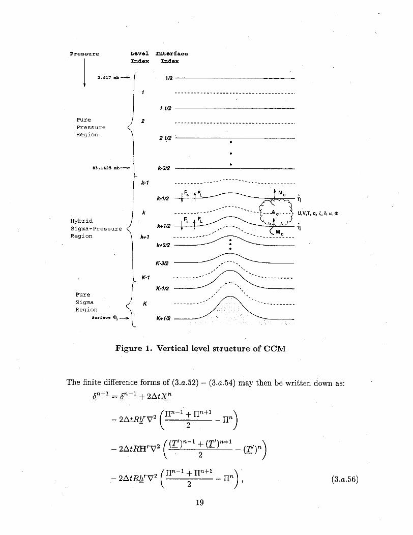
Pressure LevelIndex
2.917 mb->
1
Pure 2PressureRegion
83.1425 mb---
k-l
kHybrid
Sigma-PressureRegion k+l
K-1
Pure
Sigma KRegion
surface s -
Interface
Index
1/2
1 1/2
21/2
k-3/2
k-1/2
k+ 1/2
.
0
S
…--- -
U,V,T, q, r, S, o),
TI
k+3/2
K-3/2
K-1/2
K+1/2 :::: ---- -
K+1/2 . . ..
Figure 1. Vertical level structure of CCM
The finite difference forms of (3.a.52) - (3.a.54) may then be written down as:5n+1 = 6n-1 + 2AtX n
-2AztRbrV 2 (IIn- + In -n)· - -2
- 2tRHrV2 -- (T') - (T') )2)
- 2AtRhrV 2 (n- + n+l-_ n+ ) (3.a.56)
19
- - -

nt n - 1 + 6+ 1 _ +1
T +1 = T- 1 + 2AtY n - 2AtD" ( -n1 -- n ) (3.a.57)-2 l-
where ()n denotes a time varying value at time step n. The quantities Xnyn, and Znare defined so as to complete the right-hand sides of (3.a.43) - (3.a.45). The componentsof Apr are given by Apr = p+½ -p_ 1. This definition of the vertical difference operator
A will be used in subsequent equations. The reference matrices H' and D', and thereference column vectors bI and hr, depend on the precise specification of the verticalcoordinate and will be defined later.
Energy conservation
We shall impose a requirement on the vertical finite differences of the model thatthey conserve the global integral of total energy in the absence of sources and sinks. Weneed to derive equations for kinetic and internal energy in order to impose this constraint.The momentum equations (more painfully, the vorticity and divergence equations) withoutthe Fu, Fv, FCH and F6H contributions, can be combined with the continuity equation
9 (9p\ ( &p \ (9 (p\at rp pv+ k ) +V) 0 (3.a.59)
to give an equation for the rate of change of kinetic energy:
k( apE>-V() =-V PEV) _ (PE)
_-^ V Vp- V. V@V. (3.a.60)
The first two terms on the right-hand side of (3:a.60) are transport terms. The horizontalintegral of the first (horizontal) transport term should be zero, and it is relativelystraightforward to construct horizontal finite difference schemes that ensure this. Forspectral models, the integral of the horizontal transport term will not vanish in general,but we shall ignore this problem.
The vertical integral of the second (vertical) transport term on the right-hand sideof (3.a.60) should vanish. Since this term is obtained from the vertical advection terms formomentum, which will be finite differenced, we can construct a finite difference operatorthat will ensure that the vertical integral vanishes.
20
The vertical advection terms are the product of a vertical velocity (O10p/97]) andthe vertical derivative of a field (Ob/Op). The vertical velocity is defined in terms ofvertical integrals of fields (3.a.41), which are naturally taken to interfaces. The verticalderivatives are also naturally taken to interfaces, so the product is formed there, and thenadjacent interface values of the products are averaged to give a midpoint value. It is thedefinition of the average that must be correct in order to conserve kinetic energy undervertical advection in (3.a.60). The derivation will be omitted here, the resulting verticaladvection terms are of the form:
.OapO -0 1
VOrO ap k 2AaPk(n Op
APk -= Pk+1/2 - Pk-1/2 (3.a.62)
The choice of definitions for the vertical velocity at interfaces is not crucial to the energyconservation (although not completely arbitrary), and we shall defer its definition untillater. The vertical advection of temperature is not required to use (3.a.61) in order toconserve mass or energy. Other constraints can be imposed that result in different formsfor temperature advection, but we will simply use (3.a.61) in the system described below.
The last two terms in (3.a.60) contain the conversion between kinetic and internal(potential) energy and the form drag. Neglecting the transport terms, under assumptionthat global integrals will be taken, noting that Vp = oPVII, and substituting for thegeopotential using (3.a.40), (3.a.60) can be written as:
Oa Op E) =-ROpO \E& j-RTV.at 9 aq 1'qn (Tp an)
p 07a )
9p(1)aPv VVs - v. XV RTdlnp+ ...atr 9r) (7O)
(3.a.63)
The second term on the right-hand side of (3.a.63) is a source (form drag) term that canbe neglected as we are only interested in internal conservation properties. The last termon the right-hand side of (3.a.63) can be rewritten as
(9, p (7?)RTdlnpV * { pv j
7v fP(71)
21
(+il- k) +( 9) k-1/2\ ^/fc-l/2
(Ok-f' -k1) , (3.a.61)
RTdlnp)
V v(~V)/ R'Tdln p. (3.a.64)· ( ) JpP()
The global integral of the first term on the right-hand side of (3.a.64) is obviously zero, sothat (3.a.63) can now be written as:
t 9PE) =-RT V p - VII)
+V - V ) R Tdlnp+... (3.a.65)
We now turn to the internal energy equation, obtained by combining thethermodynamic equation (3.a.35), without the Q, FTH, and FFH terms, and the continuityequation (3.a.59):
0 (9 p Op a OpAt (7cp*T) =-V* (cTV - 8 -(PT
+ RT---. (3.a.66)C) yc p
As in (3.a.60), the first two terms on the right-hand side are advection terms that can beneglected under global integrals. Using (3.a.16), (3.a.66) can be written as:
O (O-cpT) Op V(7rp )I c*T I RT Vao q 77 p i~n
-RTfrp 1 jV V) (V dr+... (3.a.67)
The rate of change of total energy due to internal processes is obtained by adding(3.a.65) and (3.a.67) and must vanish. The first terms on the right-hand side of (3.a.65)and (3.a.67) obviously cancel in the continuous form. When the equations are discretizedin the vertical, the terms will still cancel, providing that the same definition is used for(l/p ap/O7r)k in the nonlinear terms of the vorticity and divergence equations (3.a.38) and(3.a.39), and in the w term of (3.a.35) and (3.a.42).
The second terms on the right-hand side of (3.a.65) and (3.a.67) must also cancelin the global mean. This cancellation is enforced locally in the horizontal on the columnintegrals of (3.a.65) and (3.a.67), so that we require:
=rp {RT j .p( l ) (3V{ (- h Rrd Inpd )t4 {r f -Jp7V
lnt I 9 p 7t Dan-,
22

The inner integral on the left-hand side of (3.a.68) is derived from the hydrostatic equation(3.a.40), which we shall approximate as
K
k= Ds, + R Hke Te,e=k
K
= s + R HkT7, (3.a.69)e=i.
(=I sl + RHT, (3.a.70)
where Hke = 0 for £ < k. The quantity 1 is defined to be the unit vector. The innerintegral on the right-hand side of (3.a.68) is derived from the vertical velocity equation(3.a.42), which we shall approximate as
(_)k= (--) Vk VkK 197r k r \ I
- c L6p+ (vP .+ (V ) V i( ) ,A (3.a.71)
where Cke 0 for t > k, and Cki is included as an approximation to 1/pk for e < kand the symbol A is similarly defined as in (3.a.62). Cke will be determined so that w isconsistent with the discrete continuity equation following Williamson and Olson (1994).Using (3.a.69) and (3.a.71), the finite difference analog of (3.a.68) is
{ )k [AN Pk+IVk .VHY/A ( kkiT} ALTkK:K ( [r\] k A
E = S R- AZAPCkp + T (V V) ( ) R A H Ak,(3.a.72)
where we have used the relation V * V(9p/9)k = [SkAPk + r (Vk VII) A 9p/9P/r)k]/Ark(see 3.a.22). We can now combine the sums in (3.a.72) and simplify to give
{[-- kApc +Tr(VkVII) (a ) ]Hkiti}
=E { [&AptP +7r (Vt. VII)A ( ) APkCkte k (3.a.73)
Interchanging the indexes on the left-hand side of (3.a.73) will obviously result in identicalexpressions if we require that
Hke = CekApe. (3.a.74)
23

Given the definitions of vertical integrals in (3.a.70) and (3.a.71) and of verticaladvection in (3.a.61) and (3.a.62) the model will conserve energy as long as we requirethat C and H satisfy (3.a.74). We are, of course, still neglecting lack of conservation dueto the truncation of the horizontal spherical harmonic expansions.
Horizontal diffusion
CCM3 contains a horizontal diffusion term for T,(, and 6 to prevent spectralblocking and to provide reasonable kinetic energy spectra. The horizontal diffusionoperator in CCM3 is also used to ensure that the CFL condition is not violated in theupper layers of the model. The horizontal diffusion is a linear V2 form on 77 surfaces in thetop three levels of the model and a linear V4 form with a partial correction to pressuresurfaces for temperature elsewhere. The V 2 diffusion near the model top is used as asimple sponge to absorb vertically propagating planetary wave energy and also to controlthe strength of the stratospheric winter jets. The V 2 diffusion coefficient has a verticalvariation which has been tuned to give reasonable Northern and Southern Hemispherepolar night jets.
In the top three model levels, the V 2 form of the horizontal diffusion is given by
FCH = K(2) [V 2 (( + f) + 2 (( + f) /a 2 ], (3.a.75)
F6 = K(2) [V 26 + 2(6/a 2 )], (3.a.76)
FTH = K(2)V 2 T. (3.a.77)
Since these terms are linear, they are easily calculated in spectral space. Theundifferentiated correction term is added to the vorticity and divergence diffusionoperators to prevent damping of uniform (n = 1) rotations (Orszag, 1974; Bourke etal., 1977). The V 2 form of the horizontal diffusion is applied only to pressure surfaces inthe standard model configuration.
The horizontal diffusion operator is better applied to pressure surfaces than toterrain-following surfaces (applying the operator on isentropic surfaces would be stillbetter). Although the governing system of equations derived above is designed to reduceto pressure surfaces above some level, problems can still occur from diffusion along thelower surfaces. Partial correction to pressure surfaces of harmonic horizontal diffusion
24

(Qk/Ot = KV2 ~) can be included using the relations:
Vp = V V7-p V, Inp
(3.a.78)
V = -V -_ p 7v lnp - 2V,7 (p)Vp +Pa Vq (9P cp X722P i I
Retaining only the first two terms above gives a correction to the rq surface diffusion whichinvolves only a vertical derivative and the Laplacian of log surface pressure,
V2p = V 2-1i -- PV 2HI + .. . (3.a.79)
Similarly, biharmonic diffusion can be partially corrected to pressure surfaces as:
7 p2- 74 ~' p O~r .V4 V4- 7r-- V4- +... (3.a.80)
Op Owrr
The bi-harmonic V 4 form of the diffusion operator is applied at all other levels (generallythroughout the troposphere) as
FCH = -K ( 4 [V4 ( + f) -( + f) (2/a2)2 ], (3.a.81)
FH = -K(4) [V46 - 6(2/a2) 2], (3.a.82)
FTH -K4) [V4T - T7rp --II . (3.a.83)
The second term in FTH consists of the leading term in the transformation of the V 4
operator to pressure surfaces. It is included to offset partially a spurious diffusion of Tover mountains. As with the V 2 form, the V 4 operator can be conveniently calculated inspectral space. The correction term is then completed after transformation of T and V 41back to grid-point space. As with the V2 form, an undifferentiated term is added to thevorticity and divergence diffusion operators to prevent damping of uniform rotations.
Finite difference equations
It will be assumed that the governing equations will be solved using the spectralmethod in the horizontal, so that only the vertical and time differences are presentedhere. The schematic dynamics term r in equation (2.a.3a) includes horizontal diffusionof T, (C + f), and . Only T has the leading term correction to pressure surfaces. Thus,equations that include the terms in this time split sub-step are of the form
25

= Dyn ()- (-l)iK(2i)V , (3.a.84)
for (C + f) and 6, and
9T (2i){V2 iTOT pOt= Dyn (T) - (-1)K 2 ) iV2T -7r i V 2 } , (3.a.85)
where i = 1 in the top few model levels and i = 2 elsewhere (generally within thetroposphere). These equations are further subdivided into time split components:
Xn+ = bn-1 + 2At Dyn (o n+1 n, np n - 1) , (3.a.86)
*= pn+l - 2At (-1)'K(2 )V2 (*n+l) , (3.a.87)
¢n+ l = ,* , (3.a.88)
for (C + f) and 6, and
T " + = T " - l + 2At Dyn (Tn+,T TT - l ) , (3.a.89)
T* = T + - 2At (-1)i K(2 i)V 2 i7 (T*) , (3.a.90)
n+l = T* + 2At (-1) iK(2i)r O a V 2 i n , (3.a.91)&p anr
for T, where in the standard model i only takes the value 2 in (3.a.91). The first stepfrom ( ) n - l to ( )n+l includes the transformation to spectral coefficients. The secondstep from ( )n +l to (^)n+1 for 6 and (, or ( )n+l to ( )* for T, is done on the spectralcoefficients, and the final step from ( )* to (^)n + l for T is done after the inverse transformto the grid point representation.
The following finite-difference description details only the forecast given by (3.a.86)
and (3.a.89). In what follows we use ( ) n l- instead of( ) from (2.a.8). This notationis convenient for discussing the dynamical equations in isolation. The finite-differenceform of the forecast equation for water vapor will be presented later in Section 3c. Thegeneral structure of the complete finite difference equations is determined by the semi-implicit time differencing and the energy conservation properties described above. Inorder to complete the specification of the finite differencing, we require a definition of thevertical coordinate. The actual specification of the generalized vertical coordinate takesadvantage of the structure of the equations (3.a.33) - (3.a.42). The equations can be finite-differenced in the vertical and, in time, without having to know the value of q anywhere.The quantities that must be known are p and ap/Oar at the grid points. Therefore the
26

coordinate is defined implicitly through the relation:
p(77, 7r) = A(77)po + B(V)7r,
which gives
ap
(3.a.92)
(3.a.93)
A set of levels 7k may be specified by specifying Ak and Bk, such that 77k Ak + Bk, anddifference forms of (3.a.33) - (3.a.42) may be derived.
The finite difference forms of the Dyn operator (3.a.33) - (3.a.42), including semi-implicit time integration are:
(n+l = (n- + 2Atk. V x (n n /cos ) , (3.a.94)
6n+1 = n- [V . (n-1/cos0) 2 (n + >At, + RH"n( ')]
-AtRHrV 2 ( (T'n-1 -+ (/T')n+l- 2AtRH V2 (T) 2 +-(_T,+- (T)n)
- 2AtR (br + hr) V 2 I n- 1+ n+l2
(T'n+l = (T' )n-l 2At 2[ 1a cos 2
- 2AtDr (- + n+l-((--1 2
_ r9
(UT') + - aq(VT')a cos ' O'
(3.a.95)
-rn]
_ n)(3.a.96)
in+l = nr- 1 - 2At- ((An)T Ap" + (Vn)T VIlnrniA)7rn \ -- - --- /
T-_ n-Jr
- 2 (t 6n- l + 6n+ l1AP7rr I (3.a.97)
(nu)k = (k + f)Vk-RTk(1 ap 101I\p 9r k a A
(Uk+l - Uk) +)ap (Uk - Uk-1)f kak-1/2
1 ap Cos 0 6Op (97r a ido
27
12Apk
+ (Fu)k
(nv)k= - (k +f)Uk- Rk
] (3.a.98)

77I)07/ k+1/2(Vk+l - Vk) +
Pk = T1 6k (RTk (W) Q(C;)k P k
On (T k +l - Tk)+\- '' ̂ f+ 1/ 2(r p ) (Tk- Tk-)] ,(3.a.100)
k k-l/2
Ek = (Uk) + (vk) 2 ,
RTk R ( T + Tk(C;)k cp + P _ 1 qk
'97Jk±1/2
K
= Bk+1/2 E [3eApe + Vte 7VIIABe]e=1
k
-Z [St Ape + Ve' 7rVIIABe],e=1
(p)k ()Vk /rV- Ck [ap+=Ck [ + V
£=l
1 for t < k
Ck _ I- for = k'2pk
HkU CekApt,
RD'e = Ap T C
p
Apr+ 2Ap (T k - T- 1 )2AprC
(Ekt+l - Bk-1/2)
28
12Ap+ (
+ (Fv)k ,
(3.a.99)
1
2Apk
(3.a.101)
(3.a.102)
irVITABe],
(3.a.103)
(3.a.104)
(3.a.105)
(3.a.106)
a'7lp k-1/2 .

Ž+ ^2(pr ~T~ T ) (eke- Bk+l / 2) * ((3.a.107)k
ek { ,< k (3.a.108)
where notation such as (UT') ' denotes a column vector with components (UkTk)' . Inorder to complete the system, it remains to specify the reference vector h r , together withthe term (l/p ap/i7r), which results from the pressure gradient terms and also appears inthe semi-implicit reference vector br:
lp\ (1\ 9p\ B_lp- =1 B 3k (3.a.109)p arkkP kcrJ k Pk
br = T, (3.a.110)
h =0. (3.a.111)
The matrices C' and Hn (i.e., with components Cke and Hkt) must be evaluated ateach time step and each point in the horizontal. It is more efficient computationally tosubstitute the definitions of these matrices into (3.a.95) and (3.a.104) at the cost of someloss of generality in the code. The finite difference equations have been written in theform (3.a.94) - (3.a.111) because this form is quite general. For example, the equationssolved by Simmons and Striifing (1981) at ECMWF can be obtained by changing only thevectors and hydrostatic matrix defined by (3.a.108) - (3.a.111).
b. Spectral Transform
The spectral transform method is used in the horizontal exactly as in CCM1.As shown earlier, the vertical and temporal aspects of the model are represented byfinite-difference approximations. The horizontal aspects are treated by the spectral-transform method, which is described in this section. Thus, at certain points in theintegration, the prognostic variables ( + f),, T, and H are represented in terms ofcoefficients of a truncated series of spherical harmonic functions, while at other pointsthey are given by grid-point values on a corresponding Gaussian grid. In general, physicalparameterizations and nonlinear operations are carried out in grid-point space. Horizontalderivatives and linear operations are performed in spectral space. Externally, the modelappears to the user to be a grid-point model, as far as data required and producedby it. Similarly, since all nonlinear parameterizations are developed and carried out ingrid-point space, the model also appears as a grid-point model for the incorporation
29

of physical parameterizations, and the user need not be too concerned with the spectralaspects. For users interested in diagnosing the balance of terms in the evolution equations,however, the details are important and care must be taken to understand which termshave been spectrally truncated and which have not. The algebra involved in the spectraltransformations has been presented in several publications (Daley et al., 1976; Bourkeet al., 1977; Machenhauer, 1979). In this report, we present only the details relevant tothe model code; for more details and general philosophy, the reader is referred to theseearlier papers.
Spectral algorithm overview
The horizontal representation of an arbitrary variable + consists of a truncatedseries of spherical harmonic functions,
M nV(m)
(A,/u) - E) E PmP )(/)eimA, (3.b.1)m=-M n=lmf
where g = sin X, M is the highest Fourier wavenumber included in the east-westrepresentation, and Af (m) is the highest degree of the associated Legendre polynomialsfor longitudinal wavenumber m. The properties of the spherical harmonic functions usedin the representation can be found in the review by Machenhauer (1979). The modelis coded for a general pentagonal truncation, illustrated in Figure 2, defined by threeparameters: M, K, and N, where M is defined above, K is the highest degree of theassociated Legendre polynomials, and N is the highest degree of the Legendre polynomialsfor m = 0. The common truncations are subsets of this pentagonal case:
Triangular: M = N = K,
Rhomboidal: K = N + M, (3.b.2)
Trapezoidal: N = K > M.
The quantity A((m) in (3.b.1) represents an arbitrary limit on the two-dimensionalwavenumber n, and for the pentagonal truncation described above is simply given by
/(m) = min (N + Iml, K).
The associated Legendre polynomials used in the model are normalized such that
X [Pn _()]2 d = 1 (3.b.3)-1
With this normalization, the Coriolis parameter f is
f = - P17P', (3.b.4)which is required for the absolute vorticity.
which is required for the absolute vorticity.
30

A
N
0
n
m0 M
Figure 2. Pentagonal truncation parameters
The coefficients of the spectral representation (3.b.1) are given by1 27r
Omn 2 O1 j b / (A, M)e-iAdAPn (ML)d/. (3.b.5)
The inner integral represents a Fourier transform,
1 oP2rm(l= (I) - r (A, /l)e-imdA, (3.b.6)
which is performed by a Fast Fourier Transform (FFT) subroutine. The outer integral isperformed via Gaussian quadrature,
J
An = f m(~j)Pn (Lj)wj (3.b.7)j=1
where Mj denotes the Gaussian grid points in the meridional direction, Wj the Gaussianweight at point /j, and J the number of Gaussian grid points from pole to pole. TheGaussian grid points (pj) are given by the roots of the Legendre polynomial Pj(t), and
31
4I

the corresponding weights are given by
2(1 -2)wj -[JPJ-(] 2 (3.b.8)
[JPj l()]2'
The weights themselves satisfy
J
wj = 2.0 . (3.b.9)j=l
The Gaussian grid used for the north-south transformation is generally chosento allow un-aliased computations of quadratic terms only. In this case, the number ofGaussian latitudes J must satisfy
J > (2N+K+M + 1)/2 for M <2(K-N), (3.b.10)
J > (3K + 1)/2 for M > 2(K- N). (3.b.11)
For the common truncations, these become
J > (3K + 1)/2 for triangular and trapezoidal, (3.b.12)
J > (3N + 2M + 1)/2 for rhomboidal. (3.b.13)
In order to allow exact Fourier transform of quadratic terms, the number of points P inthe east-west direction must satisfy
P> 3M +1 . (3.b.14)
The actual values of J and P are often not set equal to the lower limit in order to allowuse of more efficient transform programs.
Although in the next section of this model description, we continue to indicatethe Gaussian quadrature as a sum from pole to pole, the code actually deals with thesymmetric and antisymmetric components of variables and accumulates the sums fromequator to pole only. The model requires an even number of latitudes to easily use thesymmetry conditions. This may be slightly inefficient for some spectral resolutions. Wedefine a new index, which goes from -I at the point next to the south pole to +1 at thepoint next to the north pole and not including 0 (there are no points at the equator or polein the Gaussian grid), i.e., let I = J/2 and i = j - J/2 for j > J/2 + 1 and i = j - J/2 -1for j < J/2; then the summation in (3.b.7) can be rewritten as
I
nm E Vm (/li)P (fii)Wi. (3.b.15)i=-Ii$O
32

The symmetric (even) and antisymmetric (odd) components of Om are defined by
(E) ( + i)2
(3.b.16)
(v)r = 2 (f - 2i)
Since wi is symmetric about the equator, (3.b.15) can be rewritten to give formulas forthe coefficients of even and odd spherical harmonics:
I
IE ('bE)i (Lli)P (tli)2wi for n -m even,i=l
(=2n - (3.b.17)
E (Vo) (pi)Pm ()2wu for n - m odd.i=l
The model uses the spectral transform method (Machenhauer, 1979) for allnonlinear terms. However, the model can be thought of as starting from grid-pointvalues at time t (consistent with the spectral representation) and producing a forecastof the grid-point values at time t + At (again, consistent with the spectral resolution).The forecast procedure involves computation of the nonlinear terms including physicalparameterizations at grid points; transformation via Gaussian quadrature of the nonlinearterms from grid-point space to spectral space; computation of the spectral coefficients ofthe prognostic variables at time t + At (with the implied spectral truncation to the modelresolution); and transformation back to grid-point space. The details of the equationsinvolved in the various transformations are given in the next section.
Combination of terms
In order to describe the transformation to spectral space, for each equation wefirst group together all undifferentiated explicit terms, all explicit terms with longitudinalderivatives, and all explicit terms with meridional derivatives appearing in the Dynoperator. Thus, the vorticity equation (3.a.94) is rewritten
(+ f)+ __ '1' 2 ) V -(1 - 2) (V)] , (3.b.18)
where the explicit forms of the vectors V, V>,, and Vu are given in Appendix A [(Al)-(A3).] The divergence equation (3.a.95) is
33

?+ _=_D + (- )-(DA1 - v 2_Dvan+l -A 1 2) D +aA(1 + (1 - Ja ( ]- V(3.b.19)
- AtV 2 (RHrT 'n+l + R (br + hr) I"l+1 ).
The mean component of the temperature is not included in the next-to-last term sincethe Laplacian of it is zero. The thermodynamic equation (3.a.96) is
T" + l = T- (_ ) [ ( A) + (1 -[2) (T,)] -AtDr n+l 1 (3.b.20)a(1 - ,u2) a T
The surface-pressure tendency (3.a.97) is
n + 1 = PS -A (PrT .+ (3.b.21)
The grouped explicit terms in (3.b.19)-(3.b.21) are all given in Appendix A [(A4)-(A11)].
Transformation to spectral space
Formally, Equations (3.b.18)- (3.b.21) are transformed to spectral space byperforming the operations indicated in (3.b,22) to each term. We see that the equations
basically contain three types of terms, for example, in the vorticity equation the
undifferentiated term V, the longitudinally differentiated term Vx, and the meridionally
differentiated term VA. All terms in the original equations were grouped into one of these
terms on the Gaussian grid so that they could be transformed at once.
Transformation of the undifferentiated term is obtained by straightforwardapplication of (3.b.5) - (3.b.7),
J
{V}n = Z; Vm(/j)Pn(/Lj)wj, (3.b.22)j=1
where Vm(pj) is the Fourier coefficient of V with wavenumber m at the Gaussian grid
line /j. The longitudinally differentiated term is handled by integration by parts, using
the cyclic boundary conditions,
{ l I '2 9 Vx -iX{ } = j 2 7 r c9VAimAdA
(3.b.23)
= _ V xe- i m x dA,
34

so that the Fourier transform is performed first, then the differentiation is carried out inspectral space. The transformation to spherical harmonic space then follows (3.b.25):
{a(1 2) V) = imZ VA i) (J) (3.b.24)j=1 3
where Vy (pj) is the Fourier coefficient of VA with wavenumber m at the Gaussian gridline I 3j.
The latitudinally differentiated term is handled by integration by parts using zeroboundary conditions at the poles:
r 1· /? ma >1 2 aa(1 - 2)(1 - a2) (V = (1 I 2)(1- 2) (V d
(3.b.25)
fl 1 dP m
J a(l 2) Vm(l t 2 ) n d A.
Defining the derivative of the associated Legendre polynomial by
H m = (1- 12) dnm (3.b.26)
(3.b.28) can be written
{ 1 (1 ,2) ia (H)=-V H(VA)m H(IJ) wj. (3.b.27)a(l11OA n j=l, a(1 - 2 )j
Similarly, the V2 operator in the divergence equation can be converted to spectral spaceby sequential integration by parts and then application of the relationship
V 2pm()eim -n(n + ) m im (.28)· ) - n (/) , (3.b.28)a2
to each spherical harmonic function individually so that
{V2Dv}m = (n ) Dm()pnm(lj)wj (3.b.29)a2
j=1
where Dm (t) is the Fourier coefficient of the original grid variable _Dv.
Solution of semi-implicit equations
The prognostic equations can be converted to spectral form by summation over theGaussian grid using (3.b.22), (3.b.24), and (3.b.27). The resulting equation for absolutevorticity is
( + f)m = V (3.b.30)
where (C + f) m denotes a spherical harmonic coefficient of (C + f)n+l, and the form ofVS$, as a summation over the Gaussian grid, is given in Appendix A (A12).
35

The spectral form of the divergence equation (3.b.19) becomes
M= DS + At n [RHrTnm + R (br + hr) Ir ] (3.b.31)a 2 --
where 6m T 'm and H1 are spectral coefficients of 6n +1 T'n+l, and I n + 1. TheLaplacian of the total temperature in (3.b.19) is replaced by the equivalent Laplacianof the perturbation temperature in (3.b.31). DSm is given in Appendix A (A13). Thespectral thermodynamic equation is
T' TSm - AtDrg, (3.b.32)
with TSm defined in Appendix A (A14), while the surface pressure equation is
=P pS2-m (Apr)T t (3.b.33)
where PSn is also given in Appendix A (A15).
Equation (3.b.30) for vorticity is explicit and complete at this point. However,the remaining equations (3.b.31)-(3.b.33) are coupled. They are solved by eliminating allvariables except 6m :
AnJm = DSm + At ( +1) [RHr(TS)m + R (br + hr) (PS)n], (3.b.34)a2
where
An =I+At2 2 n ) [RHrDr+R( r +h) (( 1 (3.b. 3 5)
which is simply a set of K simultaneous equations for the coefficients with givenwavenumbers (m,n) at each level and is solved by inverting An. In order to preventthe accumulation of round-off error in the global mean divergence (which if exactly zeroinitially, should remain exactly zero) (Ao) -1 is set to the null matrix rather than theidentity, and the formal application of (3.b.34) then always guarantees P = 0. Once 6m
is known, T'm and 1m can be computed from (3.b.32) and (3.b.33), respectively, and allprognostic variables are known at time n+1 as spherical harmonic coefficients. Note thatthe mean component To is not necessarily zero since the perturbations are taken withrespect to a specified T r .
Horizontal diffusion
As mentioned earlier, the horizontal diffusion in (3.a.87) and (3.a.90) is computedimplicitly via time splitting after the transformations into spectral space and solution ofthe semi-implicit equations. In the following, the C and 6 equations have a similar form,so we write only the 6 equation:
(*) m = (Sn+ 1) -(-1) 2AtK( 2i ) [V 2i ((*) m - (-1) (6*) m (2/a2)i] (3.b.36)
(T*) - (Tn+1)m - (_l)i 2AtK( 2i ) [V 2i (T*)m] . (3.b.37)
36
The extra term is present in (3.b.36), (3.b.40) and (3.b.42) to prevent damping ofuniform rotations. The solutions are just
(5*)n = K( 2 i ) (6 n+-n1)m, (3.b.38)
(T*)m = K ( 2 i ) (T) (Tn+1 )m (3.b.39)
n 2(2) r [In (n + 1) N32 b . 1K( (6) = { + 2L\tDK 2 ) [( a2 } - } (3.b.40)
IK 2(T) ()= j1+2AtDnK 2 )( n (n + 1j)) (3.b.41)n a2
K( 4 () = { + 2AtDK 4 ) (n + 4 I() (3.b.42)n \ a2 a4
K(4) (T)= {1 + 2AtDnK(4) n (n ) } (3.b.43)n a J
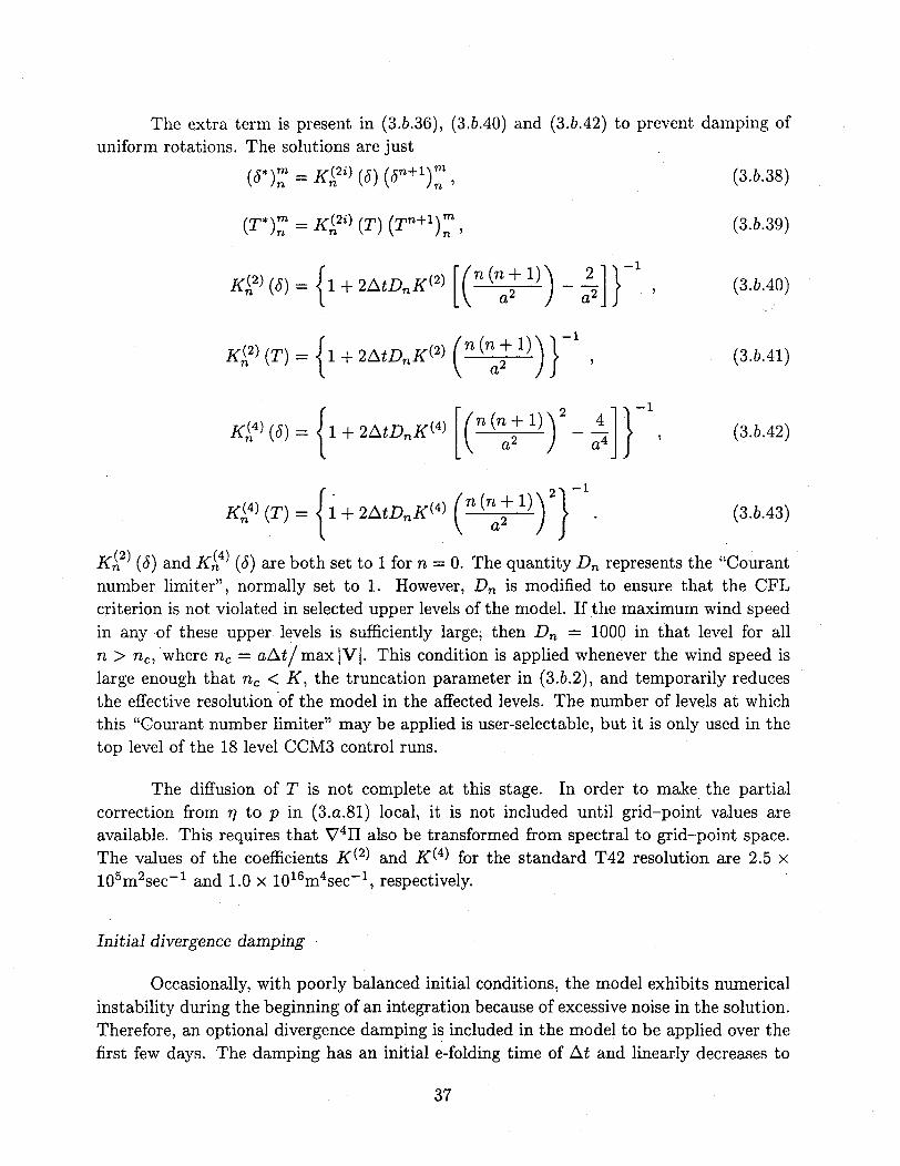
K(2) (6) and K(4) (6) are both set to 1 for n = 0. The quantity Dn represents the "Courantnumber limiter", normally set to 1. However, Dn is modified to ensure that the CFLcriterion is not violated in selected upper levels of the model. If the maximum wind speedin any of these upper levels is sufficiently large; then Dn = 1000 in that level for alln > nc, where nc = aAt/max VI. This condition is applied whenever the wind speed islarge enough that nc < K, the truncation parameter in (3.b.2), and temporarily reducesthe effective resolution of the model in the affected levels. The number of levels at whichthis "Courant number limiter" may be applied is user-selectable, but it is only used in thetop level of the 18 level CCM3 control runs.
The diffusion of T is not complete at this stage. In order to make the partialcorrection from ?7 to p in (3.a.81) local, it is not included until grid-point values areavailable. This requires that V 417 also be transformed from spectral to grid-point space.The values of the coefficients K(2) and K(4) for the standard T42 resolution are 2.5 x10⁵ m 2 sec- 1 and 1.0 x 10¹⁶ m 4 sec- 1, respectively.
Initial divergence damping
Occasionally, with poorly balanced initial conditions, the model exhibits numericalinstability during the beginning of an integration because of excessive noise in the solution.Therefore, an optional divergence damping is included in the model to be applied over thefirst few days. The damping has an initial e-folding time of At and linearly decreases to
37
0 over a specified number of days, tD, usually set to be 2. The damping is computed
implicitly via time splitting after the horizontal diffusion.
r = max 1 (t - t)/D, o] (3.b.44)
(^*) = 1 (5*)m (3.b.45)W n 1 + 2Atr n
Transformation from spectral to physical space
After the prognostic variables are completed at time n + 1 in spectral space
+f)*), (5*)m, (T*)m (Iin+l), they are transformed to grid space. For a
variable A, the transformation is given by
M FV(m)
)(A, /) = jE PE n(/)] eim x. (3.b.46)m=-M n=[lmI
The inner sum is done essentially as a vector product over n, and the outer is again
performed by an FFT subroutine. The term needed for the remainder of the diffusion
terms, V 4 n, is calculated from
v4In+l = 1 ~e n(n + 1) (/) eim x (3.b.47)-- 1)) (Ha2 )^J) emA 2n (3.b.47)'m=-M n=lml a
In addition, the derivatives of nI are needed on the grid for the terms involving VII and
VVH-aVVilU H V V
V nVH = 2) + 2(1-. (3.b.48)a(l - j2 ) 9\ all - p2) ap,
These required derivatives are given by
M [A((m)
Zt. im E HrnM P j et m,' (3.b.49)
m=-M n=lml
and using (3.b.26),
M 'V(m)n (1 21 M [=E E nHn) e1 , (3.b.50)
m=-M Ln=lmI
which involve basically the same operations as (3.b.47). The other variables needed on
the grid are U and V. These can be computed directly from the absolute vorticity and
divergence coefficients using the relations
(C + f)= n(n 2 1)z + fn, (3.b.49)a2
38

an = n(n2 ), (3.b.52)a2 Xn
in which the only nonzero fm is f- = Q//.375, and
lax _(1 _ L2 ) apU- 10X (3.b.53)
a 9A a djLz
1 a'O (1 _-/t 2) aXV = - + ( )(3.b.54)a cA a o,' "
Thus, the direct transformation is
im .1M /(m) m ( e
U = - S a n() - (n ) ( + + f)mHm() e+im=-M n=ml
a f2- Ho, (3.b.53)
2 0~.375
M A'(m)
v =M- (m [ im ( + 1f) (n P( 1 ) +(( + Hm ()] eimA*(3 b 56)Vn(n+1) n(n+1) nn
m=-M n=lml
The horizontal diffusion tendencies are also transformed back to grid space. The
spectral coefficients for the horizontal diffusion tendencies follow from (3.b.36) and (3.b.37):
FTH (T*)m = (-)i+ l K 2 i [V 2i (T*)], (3.b.57)
F, ((C + f)*)m = (-l)i+l K 2i {V2i (( + f)* (-1)/ (C + f)* (2/a2)i}, (3.b.58)
F6H (')m = (-1) K 2i {V2 (6*)- (-l) i * (2/a2)i}, (3.b.59)
using i = 1 or 2 as appropriate for the V 2 or V 4 forms. These coefficients are transformed
to grid space following (3.b.1) for the T term and (3.b.55) and (3.b.56) for vorticity
and divergence. Thus, the vorticity and divergence diffusion tendencies are converted
to equivalent U and V diffusion tendencies.
Horizontal diffusion correction
After grid-point values are calculated, frictional heating rates are determined from
the momentum diffusion tendencies and are added to the temperature, and the partial
correction of the V 4 diffusion from 77 to p surfaces is applied to T. The frictional heating
rate is calculated from the kinetic energy tendency produced by the momentum diffusion
FFH - u-lFu, (u/*)/C - vnFvH (v*)/cp, (3.b.60)
39

where Fu,, and Fv, are the momentum equivalent diffusion tendencies, determined fromFCH and FsH just as U and V are determined from ( and 6, and
Ccp c1 + (PU 1 q, +l . (3.b.61)
These heating rates are then combined with the correction,
n+1 = T, + (2A H)k + 2t (7B )K(4V 4 nl. (3.b.62)
The vertical derivatives of T* (where the * notation is dropped for convenience) are definedby
(jap 1 2 Api[ 1 +2 ( )
(7rB k 2 k [Bk+1 (Tk+1 - Tk) + Bk- (Tk -Tk-.1), (3.b.63)
The corrections are added to the diffusion tendencies calculated earlier (3.b.57) togive the total temperature tendency for diagnostic purposes:
FTH(T*)k = FTH(T*)k + (2AtFFH)k + 2AtBk yr p )k V (3.b.64)
c. Semi-Lagrangian Transport
The forecast equation for water vapor specific humidity and constituent mixingratio in the r/ system is from (3.a.36) excluding sources and sinks.
dq q VVq+ pi q = 0 (3.c.1)dt - t + V
ordq &q q
d -= 3t + V. Vq +/ - 0. =°(3.c.2)
Equation (3.c.2) is more economical for the semi-Lagrangian vertical advection, as Atdoes not vary in the horizontal, while Ap does. Written in this form, the 77 advectionequations look exactly like the a equations.
These are the necessary equations for the time split subset (2.a.3b). For simplicity,in this section we will use the notation adopted in the previous section, i.e., ( )n-l for
40

( )- of (2.a.3b) and ( )n+1 for (^)+. Thus, the tendency sources have already been addedto the time level labeled (n - 1) here. The semi-Lagrangian advection step (2.a.3b) is
further subdivided into horizontal and vertical advection sub-steps, which, in an Eulerian
form, would be written
q* qn-1 + 2At (V Vq) n (3.c.3)
and
qn +l = q* + 2At ( ) (3.c.4)
In the semi-Lagrangian form used here, the general form is
q* = Lx- (qn-), (3.c.5)
qn+l = Lv (q*). (3.c.6)
Equation (3.c.5) represents the horizontal interpolation of qn-l at the departure point
calculated assuming i7 = 0. Equation (3.c.6) represents the vertical interpolation of q* at
the departure point, assuming V = 0.
The horizontal departure points are found by first iterating for the mid-point of the
trajectory, using winds at time n, and a first guess as the location of the mid-point of the
previous time step
Ak+l = AA - n (A ) /acos o, (3.c.7)
k+l = A - Atvn (A, ) /a, (3.c.8)
where subscript A denotes the arrival (Gaussian grid) point and subscript M the midpoint
of the trajectory. The velocityh components at () are determined by Lagrange cubic
interpolation. For economic reasons, the equivalent Hermite cubic interpolant with cubic
derivative estimates is used at some places in this code. The equations will be presented
later.
Once the iteration of (3.c.7) and (3.c.8) is complete, the departure point is given
by
AD = AA - 2Atu" (AM, (M) /a cos (M, (3.c.9)
PD = AA - 2Atv' (AM, PM) /a, (3.c.10)
where the subscript D denotes the departure point.
The form given by (3.c.7) - (3.c.10) is inaccurate near the poles and thus is only
used for arrival points equatorward of 70° latitude. Poleward of 70° we transform to
a local geodesic coordinate for the calculation at each arrival point. The local geodesic
coordinate is essentially a rotated spherical coordinate system whose equator goes through
41

the arrival point. Details are provided in Williamson and Rasch (1989). The transformedsystem is rotated about the axis through (AA - , 0) and (AA + 2, 0), by an angle cPA so
the equator goes through (AA, PA). The longitude of the transformed system is chosento be zero at the arrival point. If the local geodesic system is denoted by (A', p'), withvelocities (u', v'), the two systems are related by
sin ' = sinq cos A - cos sin A'COS (A - A), (3.C.11)
sin q = sin q' cos AA + cos qs sin /A cos , (3.C.12)
sin A' cos q' = - sin (AA - A) cos b , (3.c.13)
v' cos' = = V [Cos 0 cos AA + sin q sin qA cos (AA - A)]
- usin bA sin (AA - A), (3.c.14)
u' cos A' v sin A' sin b = u cos (AA - A) + v sin q sin (A - A) . (3.C.15)
The calculation of the departure point in the local geodesic system is identical to (3.c.7) -(3.c.10) with all variables carrying a prime. The equations can be simplified by noting that
(A PA) = (0, 0) by design and u'(AA A) = U(AA,PA) and v (PA, ) = V(A,PA).The interpolations are always done in global spherical coordinates.
The interpolants are most easily defined on the interval 0 < 0 < 1. Define
0 = (XD - Xi) / (Xi+l - i), (3.C.16)
where x is either A or c and the departure point XD falls within the interval (xi,xi+i).Following (23) of Rasch and Williamson (1990) with ri = 3 the Hermite cubic interpolantis given by
qD= qi+l [3 - 20] 02 - di+l [hi02 (1 - 0)](3.c.17)
+ qi [3-2 (1 - 0)] (1 _ 0) 2 + di [hi(1 0)2
(3..17)
where qi is the value at the grid point xi, di is the derivative estimate given below, andhi = xi+ -x i.
Following (3.2.12) and (3.2.13) of Hildebrand (1956), the Lagrangian cubicpolynomial interpolant used for the velocity interpolation, is given by
2
fD = ej(XD) fi+j (3.c.18)j=-i
42

where
(XD - Xi-1) .. (XD -- Xi+j-l) (XD - Xi+j+l) . . (XD -Xi+2) 319i (XD) - (3.C. 19)
(Xi (j ) - i-.. (i+j - Xi+j- 1) (xi+j - i+j+l) ... (Xi+j - Xi+ 2 )
where f can represent either u or v, or their counterparts in the geodesic coordinatesystem.
The derivative approximations used in (3.c.17) for q are obtained by differentiating(3.c.18) with respect to XD, replacing f by q and evaluating the result at XD equal xi andxi+1 . With these derivative estimates, the Hermite cubic interpolant (3.c.17) is equivalentto the Lagrangian (3.c.18). If we denote the four point stencil (xi- 1 ,xi, xi+, xi+2) by(x1, 2, x 3, x 4 , ) the cubic derivative estimates are
(X= ( 2 - x3 ) (X 2 - X4)(x - 2) (x - x 3 ) ( 1 - X4) J
[ 1 _ 1 _ 1 1
-(Xl X2) (X2 -X3) (X2 -X4) 2](3.c.20)
[ (X1 - X3) (X2 - X3) (X3 - X4) q a
(X2-X1) (X2-X 3 )
(X1 - X4) (X2- 4) (X3 - 4)
and
d= [- (x 3 -x2) (X 3 - x4) ]( - x 2) (x21 - x3 ) (x21 -xX - ) ( - 4) J
(X1 -X2) (X2 - X3) (X2 - qX4) 2 3 .(3.c.21)
[(X 1 -3) + (X2 - 3) (x 3 -X4) q3
[ (X3 - Xi) (X 3 - X 2 ) 1(X - X4) (X2 - X4) (X3- 4) q4
The two dimensional (A, S) interpolant is obtained as a tensor product applicationof the one-dimensional interpolants, with A interpolations done first. Assume thedeparture point falls in the grid box (Ai, Ai+ 1 ) and (ypi, ,°i+i). Four A interpolations areperformed to find q values at (AD, pj-i), (AD, j) ,(AD, soj+l), and (AD, Tj+2). This isfollowed by one interpolation in Sp using these four values to obtain the value at (AD, WD).
43
Cyclic continuity is used in longitude. In latitude, the grid is extended to include a polepoint (row) and one row across the pole. The pole row is set equal to the average of therow next to the pole for q and to wavenumber 1 components for u and v. The row acrossthe pole is filled with the values from the first row below the pole shifted wr in longitudefor q and minus the value shifted by ir in longitude for u and v.
Once the departure point is known, the constituent value of q* = q- 1 isobtained as indicated in (3.c.5) by Hermite cubic interpolation (3.c.17), with cubicderivative estimates (3.c.18) and (3.c.19) modified to satisfy the Sufficient Condition forMonotonicity with C° continuity (SCMO) described below. Define Aiq by
qi+l - qiAiq= - (3.c.28)
Xi+l - Xi
First, if Aiq = 0 then
di di+ =0 . (3.c.29)
Then, if either
di0 < 3 (3.c.30)
or
di+l0 < i+ < 3 (3.c.31)iAq
is violated, di or dil is brought to the appropriate bound of the relationship. Theseconditions ensure that the Hermite cubic interpolant is monotonic in the interval [xi, xi+1].
The horizontal semi-Lagrangian sub-step (3.c.5) is followed by the vertical step(3.c.6). The vertical velocity i is obtained from that diagnosed in the dynamicalcalculations (3.a.93) by
M =k (i+ d / (Pk+l-p) (3.c.32)(Op \/ (pk+ -- k
with r7 k = Ak+Bk. Note, this is the only place that the model actually requires an explicitspecification of r7. The mid-point of the vertical trajectory is found by iteration
klk = 7A A (Ai ) . (3.C.33)
Note, the arrival point 'TA is a mid-level point where q is carried, while the i7 used for theinterpolation to mid-points is at interfaces. We restrict IrM by
'1 < niM <• 7K, (3.c.34)
which is equivalent to assuming that q is constant from the surface to the first modellevel and above the top q level. Once the mid-point is determined, the departure point iscalculated from
r/D = r]A - 2Atn (riM), (3.c.35)
44

with the restriction
r71 < ?iD 71K. (3.c.36)
The appropriate values of 77 and q are determined by interpolation (3.c.17), with the
derivative estimates given by (3.c.18) and (3.c.19) for i = 2 to K - 1. At the top and
bottom we assume a zero derivative (which is consistent with (3.c.34) and (3.c.36)), di = 0
for the interval k = 1, and 6i+1 = 0 for the interval k = K 1. The estimate at the
interior end of the first and last grid intervals is determined from an uncentered cubic
approximation; that is di+1 at the k = 1 interval is equal to di from the k = 2 interval,
and di at the k = K -1 interval is equal to di+i at the k = K - 2 interval. The monotonic
conditions (3.c.30) to (3.c.31) are applied to the q derivative estimates.
d. Mass fixers
The fixers which ensure conservation (2.a.4) are applied to the dry atmospheric
mass, water vapor specific humidity and constituent mixing ratios. For water vapor and
atmospheric mass the desired discrete relations, following Williamson and Olson (1994)
are
I/ +- q+ + =P, (3.d.1)
2 3
++ = J q-Ap-, (3.d.2)
3 3
where P is the dry mass of the atmosphere. From the definition of the vertical coordinate,
Ap = poAA + rAB, (3.d.3)
and the integral f denotes the normal Gaussian quadrature while f includes a vertical2 3
sum followed by Gaussian quadrature. The actual fixers are chosen to have the form
,r+ (A, p) = Mir+ (A, ) , (3.d.4)
preserving the horizontal gradient of II, which was calculated earlier during the inverse
spectral transform, and
q+ (A, p, 7) = q+ + ariq^q - q-l. (3.d.5)
In (3.d.4) and (3.d.5) the ( ) denotes the provisional value before adjustment. The form
(3.d.5) forces the arbitrary corrections to be small when the mixing ratio is small and when
the change made to the mixing ratio by the advection is small. In addition, the 77 factor is
included to make the changes approximately proportional to mass per unit volume (Rasch
et al., 1995). Satisfying (3.d.1) and (3.d.2) gives
45

f q-Ap- - f q+poAA - M fq'+-+ABl +--poA+M l +- +AB (3.d.6)3 . 3f vq+ jqj+ - qI poAA + Mf 77+ I+ - q- +AB (3.d.6)
3 3
and
M = P+ q-Ap- / + (3.d.7)
3 2
Note that water vapor and dry mass are corrected simultaneously. Additional advectedconstituents are treated as mixing ratios normalized by the mass of dry air. This choicewas made so that as the water vapor of a parcel changed, the constituent mixing ratioswould not change. Thus the fixers which ensure conservation involve the dry mass of theatmosphere rather than the moist mass as in the case of the specific humidity above. LetX denote the mixing ratio of constituents, then the desired relationship for conservation is
J -X(1 -q+A += X-(1 -)Ap- (3.d.8)3 3
Following Rasch et al. (1995) the change made by the fixer is the same form as (3.d.5)
X+ (A, C, r) = x+ + axr + Ix+ - - I (3.d.9)
Substituting (3.d.9) into (3.d.8) and using (3.d.4) through (3.d.7) gives
fx-(l-q-)Ap-- f X+(1 - q+)A++a f X+r+lq+ - q-lAp3 A,B A,B (.
x S +I+ - X- 1 -(l -+)Aap - a Vr+1X+- X- rlq+I+ - q-lApA,B A,B
where the following shorthand notation is adopted
A ()Ap = 3( )po+M ( B (3.d.1)A,B 3 3
46

4. MODEL PHYSICS
4.1 Tendency Physics
As discussed earlier, the tendency physics include (in the following order) theparameterization of cloud amount; the evaluation of radiative fluxes and atmosphericheating rates; the evaluation of surface fluxes; update land surface properties; evaluationof free atmosphere vertical diffusivities, diagnosis of the PBL height, PBL diffusivities andnon-local transport term followed by the vertical diffusion solution; evaluation of gravitywave drag tendencies; and Rayleigh friction. Note that for greater stability the formulationof many of these processes is implicit, and the time step is further sub-divided into timesplit steps for each component to make the solution of the tendency terms more practical.The final result of the evaluation of these processes is the net tendency attributable tothe tendency physics as shown in (2.a.7). Also note that we use the more conventional Ps
notation for surface pressure (as opposed to 7r) for the following model physics discussion.
a. Cloud Parameterization
Cloud amount (or cloud fraction), and the associated optical properties, areevaluated via a diagnostic method in CCM3. Although the basic approach is similarto what was employed in the CCM2, the specific techniques represent some of the moresignificant changes to the collection of model physics. The diagnosis of cloud fractionrepresents a generalization of the scheme introduced by Slingo (1987), and depends onrelative humidity, vertical velocity, atmospheric stability, and the convective mass fluxassociated with parameterized moist convection (sections 4g and 4h). Three types ofcloud are diagnosed by the scheme: convective cloud, layered cloud, and low-level marinestratus. Some of the major changes from Slingo (1987) are: clouds are allowed to formin any model layer, except the layer nearest the surface; low-level frontal clouds occur forall w < wc (where wc is an arbitrary threshold); the relative humidity thresholds for mid-and upper-level layered clouds are functions of atmospheric stability; and convective cloudamount is determined from the rate of convective overturning (as opposed to convectiveprecipitation rate). The minimum convective cloud fraction requirement of 20% employedin the CCM2 has been removed.
Total column convective cloud amount is diagnosed from the presence and strengthof moist convective activity. In particular, it is a function of the column averagedconvective mass flux diagnosed by the moist convective parameterization (e.g., along thelines of Xu and Krueger, 1991) where
Aconv= 0.035 ln(1.0 + Mc) , (4.a.1)
47

where the vertically averaged convective mass flux Mc is given by_ rps rps
Mc = mc(p)dp/ dp, (4.a.1.1)PT PT
mc(p) is in units of mb/day, and Aonv is not allowed to exceed 80%. The convective cloudamount in each model layer is assumed to be randomly overlapped within the convectivelyactive region, the bounds of which are provided by the moist convection parameterization.Thus, the total cloud fraction in (4.a.1) is distributed in the vertical according to
Aconv = 1.0 - (1.0 - Aconv )/N, (4.a.2),
where N is the number of model levels within the convectively active region. For thesubsequent cloud fraction calculation, the large scale relative humidity within the gridbox is adjusted to account for the assumption that the fraction of convective cloud, Aconv,is saturated. The specific humidity grid value itself is unchanged. Thus, the adjusted largescale relative humidity, RH', is given by
R H - AconvRH= RH-Ac (4.a.3)1 - Aconv
where RH is the actual grid box relative humidity. The remaining cloud types arediagnosed on the basis of RH . Frontal and tropical low cloud fraction, i.e., cloudsoccurring below 750 mb, are diagnosed according to
0 w > Wc
Wc- R-H -RH',
AC ) 1- R H nO ) 0 < w (4.a.4)
RH -RHm\l 1-RHOw W < 01-RH inOw
while stratus associated with low-level inversions is determined from
Ac =
0 RH < 0.6
(-6.67p -0.667)x (1- 0o.9RH') x (P-75)
0.6 < RH' < 0.9 and
(4.a.5)op < -0.125,750 < p 900
(-6.67a - 0.667)x (75 0 ) RH' > 0.9 and
ae <-0.125-r
where as is the maximum inversion strength and RH' is the adjusted layer relative
humidity given by (4.a.3). The pressure factor, (P1 5 0 ), accounts for the transitionfrom marine stratus clouds that occur in the presence of low level inversions to tradecumulus clouds that can occur for higher level inversions. The parameter w, is set to
48

50 mb/day, allowing low level clouds to form under weak subsidence conditions. Theparameter RH,?,, the relative humidity threshold for low cloud formation, is assumed tobe 0.9 (i.e., 90%) over open ocean, and 0.8 over land. This distinction is made to accountfor enhanced cloud drop nucleation (i.e., at lower relative humidities) that can occur overCCN rich land areas.
Middle and upper level cloud is defined to occur between 750 mb and the uppermostmodel level (which relaxes an earlier constraint that clouds form only in the troposphere).Mid- and high-level stratified (or layered) cloud amount is determined from the relation
c-[maxl RH' - RHJlim 2Ac max ( 0, 1R Rim X (4.a.7)
RHim= .999 - (1 - Rhi ) [ 3] (4.a.8)3.5 x 10⁻⁴
where N 2 is the square of the Brunt-Vaisalla frequency:
2 g 2p 00N 2 = _(4.a.9)-0 ap'
Note that the ratio N 2 /3.5 x.10- 4 is not allowed to exceed 1. The parameter RH hi, therelative humidity threshold for mid-level and high cloud formation, is assumed to be 0.9(i.e., 90%). The cloud cover in any layer is finally defined as
Ac = (1.0- Aconv)Ac + Acov, (4.a.10)
where Ac is not allowed to exceed 0.999.
As in the CCM2, cloud optical properties in the CCM3 are accounted for usingthe Slingo (1989) parameterization for liquid water droplet clouds. This scheme relatesthe extinction optical depth, the single-scattering albedo, and the asymmetry parameterto the cloud liquid water path and cloud drop effective radius (see Section 4b). Thelatter two microphysical cloud properties were statically specified in the CCM2. Inparticular, in-cloud liquid water paths were evaluated from a prescribed, meridionallyand height varying, but time independent, cloud liquid water density profile, pe(z). whichwas analytically determined on the basis of a meridionally specified liquid water scaleheight (e.g., see Kiehl et al., 1994; Kiehl, 1991). The cloud drop effective radius wassimply specified to be 10am for all clouds. The CCM3 continues to diagnose cloud opticalproperties, but relaxes the rigid CCM2 framework. CCM3 employs the same exponentiallydecaying vertical profile for in-cloud water concentration
Pe = Pe(- / h ) (4.a.11)
where the reference value pe is equal to 0.21 g m -3 . Instead of specifying a zonallysymmetric meridional dependence for the cloud water scale height, hi, it is locally
49

diagnosed as a function of the vertically integrated water vapor (precipitable water)
h = 7001n (.0+- qdp (4.a.12)g T
The cloud water path is then determined by integrating the liquid water concentrationusing
CWP= JPedZ, (4.a.13)
which can be analytically evaluated for an arbitrary layer k as
e k- O1-,I+ ,+½h, -z hiCWP (k) = p°ht [ez+ - e zk/] , (4.a.14)
where zk+i and Zk-_ are the heights of the kth layer interfaces.
Observational studies have shown a distinct difference between maritime andcontinental effective cloud drop size, re, for warm clouds. For this reason, the CCM3differentiates between the cloud drop effective radius for clouds diagnosed over maritimeand continental regimes (Kiehl, 1994). Over the ocean, the cloud drop effective radius forliquid water clouds, ree, is specified to be 10[pm, as in the CCM2. Over land masses ree isdetermined using
5 f/m T > -10°C
ree = -5- (T+°) tm -30°C < T < -10°C (4.a.14.1)
Trei T < -30°CAn ice particle effective radius, rei, is also diagnosed by CCM3, which at the momentamounts to a specification of ice radius as a function of normalized pressure
10 Lm P/Ps > Pi g h
r m = e [- i. p ig}W (4. a.15.1)max max _ min (P/Ps)-Pigh high
re i = e i - ,i L high low m P/Ps 4 Pi
where rax = 30/rm, r = 10/rm, pih = 0.4, and po - 0.0. The fraction of the totalcloud water in the form of ice particles is then determined using
0 T > -10°C
fice = -0.05 (T + 10) -30°C < T < -10°C (4.a.16.1)
1 T < -30°C
Finally, for diagnostic purposes, the CCM3 calculates three levels of cloud fraction,assuming random overlap. These diagnostics, denoted as low, middle, and high cloud, arebounded by the pressure levels p, to 700 mb, 700 mb to 400 mb, and 400 mb to the modeltop.
50

b. Parameterization of Radiation
Diurnal cycle
In the standard configuration, both the longwave and shortwave heating ratesare evaluated every model hour as discussed in the following sections. Between hourlyevaluations, the longwave and shortwave fluxes and heating rates are held constant. Thesurface radiative fluxes are also fixed between hourly calculations.
The insolation at the top of the model atmosphere is given by
SI = Soe cos(, (4.b.1)
where So is the solar constant, C is the solar zenith angle, and C is the eccentricity factor(square of the ratio of mean to actual distance that depends on the time of year). Werepresent the annual and diurnal cycle of solar insolation with a repeatable solar yearof exactly 365 days and with a mean solar day of exactly 24 hours, respectively. Therepeatable solar year does not allow for leap years. The expressions defining the annualand diurnal variation of solar insolation are given by:
cos C = sin 0 sin 6 - cos q cos S cos(27rtlocal)
e = 1.000110 + .034221 cos 00 + .001280 sin 00 + .000719 cos 200 + .000077 sin 200
6 = .006918 - .399912 cos 0o + .070257 sin 00 - .006758 cos 20o+
.000907 sin 200 - .002697 cos 30o + .001480 sin 300
where27wd
= d- (mean orbit angle)365
andd = calendar day of year(= 0, for January 1 and 364 for December 31)
b = latitude in radians
6 = solar declination in radians
tlocal = calendar day with local time (ranges from 0.0 to 365.0).
Note that the calendar day d varies continuously throughout the repeatable year and isupdated every model time step.
The expression for cos was taken from Sellers (1965, p.15), while the expressionsfor e and 6 were obtained from Paltridge and Platt (1976), pages 57 and 63, respectively.The eccentricity factor e is appropriate for the current earth orbit and, according toPaltridge and Platt (1976), is accurate to better than 10 - 4 . Maximum eccentricity factor
51

(the orbit point closest to the sun (perhelion)) occurs about January 3 (calendar day 2.0),and minimum e (the orbit point farthest from the sun (aphelion)) occurs about July 5
(calendar day 185).
The declination 6 (the angle between the celestial equator and the sun) is
appropriate for the present earth obliquity of about 23 °. The declination expressionabove is accurate to better than 3' of arc (Paltridge and Platt, 1976); since the change
in declination in 24 hours is never greater than 30' of arc, (and remembering that the
disc of the sun itself subtends an angle of ' 30' of arc), the above expression is quite an
adequate approximation. Minimum declination 6 occurs on about December 22 (calendar
day 355.0), and maximum declination 6 occurs on about June 21 (calendar day 172.0).
It does not seem necessary to compute solar insolation more accurately (for
example, accounting for equation of time changes in the solar day during the year, or
accounting for long-term secular changes in orbit) for two reasons: (1) the solar insolation
given above multiplies approximate factors dealing with the scattering and absorption in
the model's atmosphere/surface system (for example, the surface albedos in the model
are not known to an accuracy of better than 1-2% of solar insolation (Briegleb et al.,
1986), and (2) for multi-year model runs, it is desirable when looking at interannual
variability that the solar insolation repeat precisely every year in order to eliminate this
source of variation. The loss (in a run of larger than 4 years) of the leap year day seems
an acceptable approximation since this loss would only amount to 5 days after a 20-year
run, for example.
The local time (tiocal) in the expression for cos depends on the calendar day as
well as model longitude:A
tlocal = d+ (4.b.2)3600'
where A = model longitude in degrees starting from Greenwich running eastward. This
would mean, for example, that a model calendar day d having no fraction (such as 182.00)
would refer to local midnight at Greenwich, and to local noon at the date line (180°
longitude).
Solar radiation
The 6-Eddington approximation of Joseph, Wiscombe, and Weinman (1976) and
also Coakley, Cess and Yurevich, (1983) has been adopted and is described in Briegleb
(1992). This approximation has been shown to simulate quite well the effects of multiple
scattering.
The solar spectrum is divided into 18 discrete spectral intervals (7 for 03, 1 for the
visible, 7 for H 2 0, and 3 for C0 2). The CCM3 model atmosphere consists of a discrete
52

vertical set of horizontally homogeneous layers within which radiative heating rates areto be specified (see Figure 1). Each of these layers is considered to be a homogeneouscombination of several radiatively active constituents. Solar irradiance, as well as surfacereflectivity for direct and diffuse radiation in each spectral interval, are specified, as wellas the cosine of the solar zenith angle.
The method involves evaluating the 3-Eddington solution for the reflectivity andtransmissivity for each layer in the vertical. The layers are then combined together,accounting for multiple scattering between layers, which allows evaluation of upward anddownward spectral fluxes at each interface boundary between layers. This procedure isrepeated for all spectral intervals to accumulate broad band fluxes, from which the heatingrate can be evaluated from flux differences across each layer.
The 5-Eddington approximation allows for gaseous absorption by 03, CO 2, 02, andH 2 0. Molecular scattering and cloud water droplet scattering/absorption are included.A summary of the spectral intervals and the absorption/scattering data used in theformulation is given in Briegleb (1992).
For cloud scattering and absorption, the radiative parameterization of Slingo [1989]for liquid water droplet clouds is employed. In this parameterization, the optical propertiesof the cloud. droplets are represented in terms of the prescribed cloud water path (CWPin units of kg m - 2, see 4.a.11-14) and effective radius, re = f r3 n(r)dr/ f r2n(r)dr, wheren(r) is the cloud drop size distribution over radius r.
Cloud radiative properties explicitly account for the phase of water. For shortwaveradiation we use the following generalization of the expression used by Slingo (1989)for liquid water clouds. The cloud liquid optical properties, for each spectral interval,(extinction optical depth, single scattering albedo, asymmetry parameter and forwardscattering parameter) are defined as,
rf = CWP 1a + b} (1-fice) (4.b.3)[ l rel
aWc= 1- c- dre (4.b.4)
S = el + ffrel (4.b.5)
ffc (g) 2 (4.b.6)
where superscript i denotes spectral interval. The spectral intervals and coefficients forliquid water are defined in Briegleb (1993). The radiative properties of ice cloud aredefined by,
,ric =CWP [a + K (4.b.7)L rei J
53

c 1 - cC - direi (4.b.8)
gi = e+ + firei (4.b.9)
fC= (j) 2 (4.b.10)
where the subscript i denotes ice radiative properties. The values for the coefficients a - fare based on the results of Ebert and Curry (1992) and are listed in Table 4.1 for thefour pseudo-spectral intervals (.25-.69 um, .69-1.19 tum, 1.19-2.38 ttm, and 2.38-4.00 rm)employed in the CCM3 shortwave radiation model. Note that when 0 < fice < 1, then thecombination of these expression in (4.b.11 - 4.b.14) represent the radiative properties for amixed phase cloud.
TABLE 4.1: Cloud ice radiative coefficients
Interval a b c d
1 3.448 x 10- 3 2.431 1.0 x 1.0- 5 02 3.448 x 10- 3 2.431 1.1 x 10- 4 1.405 x 10- 5
3 3.448 x 10- 3 2.431 1.861 x 10⁻² 8.328 x 10- 4
4 3.448 x 10- 3 2.431 0.46658 2.05 x 10- 5
Partial cloudiness and cloud overlap radiative effects are represented in thefollowing manner. A parameterization that gives results approximately equal to therandom overlap assumption, without the computational cost of calculating the spectrumof cloud cases and which gives the proper limits of zero cloud cover and complete cloudcover in a single layer, is utilized. The cloud extinction optical depth (rc) for each layer is
3modified as: rT -= TcAj and Ac is the fractional cloud cover in the layer; the power 3 wasfound necessary to give results approximately the same as the random overlap assumption.Despite the simplicity of this assumption for dealing with partial cloud cover and cloudoverlap effects, the resulting heating rates in a cloudy atmosphere are well representedwhen compared with the benchmark calculations [see Briegleb, 1992].
A uniform (in space and time) background boundary layer aerosol is included inCCM3. The aerosol is well mixed in the bottom three layers of the model. The aerosolmass mixing ratio in these layers is specified to yield a visible optical depth of 0.14. Weview this prescription of aerosol as a "place holder" for future implementations of variousaerosol types that have realistic spatial and temporal variability. The optical propertiesof the aerosol are identical to sulfate aerosols described by Kiehl and Briegleb (1993).
The 6-Eddington scheme is implemented so that the solar radiation is evaluatedonce every model hour over the sunlit portions of the model earth. The surface albedois specified in two wavebands (0.2-0.7 /m, and 0.7-5.0 um) and distinguishes albedos for
54

direct and diffuse incident radiation. Albedos for ocean surfaces, geographically varyingland surfaces, and sea ice surfaces are distinguished. Ozone is prescribed, and CO2 isassumed to be uniformly mixed with constant mass mixing ratio. Diagnostic cloud amount(Ac) is evaluated every model hour just prior to the solar radiation calculation.
For some diagnostic purposes, such as estimating cloud radiative forcing (Kiehl andRamanathan, 1990) a clear-sky absorbed solar flux is required. A diagnostic calculation isincluded to give an estimate of clear-sky column absorbed and surface absorbed flux. Forcomputational efficiency, the clear sky top of atmosphere and surface fluxes are evaluatedassuming two homogeneous atmospheric layers. The top layer contains only 03, whilethe lower layer contains all other absorbers/scatterers except clouds. The actual surfacealbedos are employed.
Details of the implementation are as follows. The CCM3 model atmosphere isdivided into K + 1 layers in the vertical; an extra top layer (beyond the K layers specifiedby CCM3) is added. This extra layer prevents excessive heating in the top layer whenthe top pressure is not very low; also, as the model does not specify absorber propertiesabove its top layer, the optical properties of the top layer must be used for the extralayer. Layers are assumed to be horizontally and vertically homogeneous for each modelgridpoint and are bounded vertically by layer interfaces. For each spectral band, upwardand downward fluxes are computed on the layer interfaces (which include the surface andtop interface). The spectral fluxes are summed and differenced across layers to evaluatethe solar heating rate. The following discussion refers to each of the spectral intervals.
In general, several constituents absorb and/or scatter in each homogeneous layer(e.g. cloud, aerosol, gases...). Every constituent is defined in terms of a layer extinctionoptical depth r, single scattering albedo w, asymmetry parameter g, and the forwardscattering fraction f. To define bulk layer properties, the combination formulas of Cess[1985] are used:
T = ZTi, (4.b.11)i
W = E i Wi, (4.b.12)T
g= (4.b.13)
Ei fiWirif= efIrI (4.b.14)
where the sums are over all constituents.
55

The 6-Eddington solution for each layer requires scaled properties for r, w, g, givenby the expressions:
r* = r(1 - f), (4.b.15)
w* = W ( 1 -f) , (4.b.16)
gl-f9 = -f (4.b.17)
1-fThe scaling accounts for the scattering effects of the strong forward peak in particle
scattering. The 6-Eddington nonconservative (w < 1) solutions for each layer for directradiation at cosine zenith angle po are (following the notation of Coakley, Cess, andYurevich, 1983):
R(po) = (a - 7)Te-/ + (a + )R- (a - 7), (4.b.18)
T(([o) = (a + y)T + (a - y)Re-7~' / ° - (a + y - 1)e-r'/ °, (4.b.19)
= (u + 1)(u - )(e xAr - e-A*)N- 1 , (4.b.10)
T= 4uN-1 , (4.b.21)
where
a- o- w3 ( 1 g*( 21 - *)) (4.b.22)
a lw3* (13 (w*)/z ) (4.b.23)
N = (u + 1) 2e ' - (u - 1)2 e-A*, (4.b.24)
2 ( A )' (4.b.25)
A = 3(1- w*)(1 - w*), (4.b.26)
where R(po), T(/Lo) are the layer reflectivity and transmissivity to direct radiationrespectively, and R, T are the layer reflectivity and transmissivity to diffuse radiationrespectively. It should be noted that in some cases of small but nonzero w, the diffuse
reflectivity can be negative. For these cases, R is set to 0, which produces negligible
impact on fluxes and the heating rate.
To combine layers, it is assumed that radiation, once scattered, is diffuse and
isotropic (including from the surface). For an arbitrary layer 1 (or combination of layerswith radiative properties RW([o), T([to)R 1,T 1) overlying layer 2 (or combination of layerswith radiative properties R 2 ( 0o), T 2 ([lto), and R 2, T 2 ), the combination formulas for direct
56

and diffuse radiation incident from above are:
R12 (o) = R1 (Ho)
+ T1{(T i(o) - e- ;/o)R2 + e-r;/1o R 2 ([o)}+1 - RR 2 , (4.b.27)1 - R1R2
T 12 (0o) = e-r;i/°T2(Po)
+T2 -eO /*IA) + e-T;/IOR 2(o) Rl}(~~1-RR+ 2 ,(4.b.28)
1- R1R2
T 1R 2T 1R 12 = R + (4.b.29)1 - R1R2
T1T2T12 = 1 RR (4.b.30)
Note that the transmissions for each layer (T 1 (o), T2 ([lo)) and for the combinedlayers (T 12 ([o)) are total transmissions, containing both direct and diffuse transmission.Note also that the two layers (or combination of layers), once combined, are no longer ahomogeneous system.
To combine the layers over the entire column, two passes are made through thelayers, one starting from the top and proceeding downward, the other starting from thesurface and proceeding upward. (In passing from the top down, the layer 5-Eddingtoncomputation of R([Lo), T(,uo), R, T is terminated if the total transmission to directradiation for the spectral band (normalized to 1.0 at top) is less than .001; this produces anegligible error and saves computational overhead). The result is that for every interface,the following combined reflectivities and transmissivities are available:
e - ' / °o- direct beam transmission from top of at-mosphere to the interface (r* is the scaledoptical depth from top-of-atmosphere tothe interface),
Rup(pIo) = reflectivity to direct solar radiation ofentire atmosphere below the interface,
Tdn(PO) = total transmission to direct solar ra-diation incident from above to entireatmosphere above the interface,
Rp = reflectivity of atmosphere below the inter-face to diffuse radiation from above,
Rdn = reflectivity of atmosphere above the inter-face to diffuse radiation from below.
57

With these quantities, the upward and downward fluxes at every interface canbe computed. For example, the upward flux would be the directly transmitted flux(e -r*/ °0) times the reflection of the entire column below the interface to direct radiation(RJup(po)), plus the diffusely transmitted radiation from above that reaches the interface(Tdn(bLO) - e-T*/° 0) times the reflectivity of the entire atmosphere below the interface todiffuse radiation from above (Rup), all times a factor that accounts for multiple reflectionsat the interface. A similar derivation of the downward flux is straightforward. Theresulting expressions for the upward and downward flux are:
Fu= e-'/oRup (Lo) + (Tdn(Ao) - e*o)Rup (4.b.31)1 - RdnRup
Fdn = e-
+(Tdn (o) - e- T /o) + e-r / -o R (o)Rd (4.b2)+ (4.b.32)1- RdnRup
The upward and downward spectral fluxes at each interface are summed to evaluatethe spectrally integrated fluxes, then differenced to produce the solar heating rate,
g Fdn (k+l) - Fup (Pk+l) - Fdn (Pk) + Fup (Pk)Qsol - C-- ------ Pk (4.b.33)Cp Pk+1 - Pk
which is added to the nonlinear term (Q) in the thermodynamic equation.
Longwave radiation
The method employed in the CCM to represent longwave radiative transfer is basedon an absorptivity/emissivity formulation (Ramanathan and Downey, 1986),
p
FL(p) = B(O)e(O,p) + Ja(p,p')dB(p') (4.b.34)0
Ps
F (p) = B(Ts) - (p p')dB(p') (4.b.35)
P
where B(T) = aT 4 , is the Stefan-Boltzmann relation. a and e are the absorptivity andemissivity,
00
f {dB,(p')/dT(p')} (1 - Tv(p,p')) dv
C(p, pl)_ o (4.b.36)(p' = dB(p')/dT(p') (436)
f B(T,) (1 - T,(O,p))dv(O,p) =- B (4.b.37)
B(0)
58

where the integration is over wavenumber, v. B (p) is the Planck function, and Tv is theatmospheric transmission. Thus, to solve for fluxes at each model layer we need solutionsto the following,
0
jI1 TV)F(BV^ (4.b.38)o
where F(BV) is the Planck function for the emissivity, or the derivative of the Planckfunction with respect to temperature for the absorptivity.
The general method employed for the solution of (4.b.38) for a given gas is basedon the broad band model approach described by Kiehl and Briegleb (1991) and Kiehl andRamanathan (1983). This approach is based on the earlier work of Ramanathan (1976).The broad band approach assumes that the spectral range of absorption by a gas is limitedto a relatively small range in wavenumber, v, and hence, can be evaluated at the bandcenter, i.e.
rV2 V2
/ (1 - T)F (Bv) dv F B) (1 - Tv)dv = F(Bo)A (4.b.39)1 M1
where A is the band absorptance (or equivalent width) in units of cm - 1. Note that A,in general, is a function of the absorber amount, the local emitting temperature, and thepressure. Thus, the broad band model is based on finding analytic expressions for theband absorptance. Ramanathan (1976) proposed the following functional form for A,
uA(u,T,P) = 2Ao0 n {1+ /4 ( /)} (4.b.40)
~S(T)where Ao is an empirical constant, u is the scaled dimensionless path length,
u= AS(T) (4.b.41)
where S(T) is the band strength, 1 is the mass mixing ratio of the absorber, pa is thedensity of air. 3 is a line width factor,
S ui d r7(T) Po d (4.b.42)
where y(T) is the mean line halfwidth for the band, P is the atmospheric pressure andPo is a reference pressure and d is the mean line spacing for the band. The determinationof y, d, S from spectroscopic line databases, such as the FASCODE database is describedin detail in Kiehl and Ramanathan (1983). Kiehl and Briegleb (1991) describe how(4.b.40) can be extended to account for sub-bands within a spectral region. Essentially,the argument in the log function is replaced by a summation over the subbands. Thisbroad band formalism is employed for C0 2, 03, CH4, N20 and minor absorption bands ofC0 2, while for the CFCs we employ the exponential transmission approximation discussed
59
by Ramanathan et al. (1985),
T = exp [-D (S(T)/Av) W] (4.b.43)
where Av is the band width, and W is the absorber path length,
W = J ppadz, (4.b.44)
and D is a diffusivity factor. The final problem that must be incorporated into the broadband method is the overlap of one or more absorbers within the same spectral region.Thus, for the wavenumber range of interest, namely 500 to 1500 cm- 1, the radiative fluxis determined in part by the integral,
(1500
J ( -T) F (B,)dv (4.b.45)500
which can be re-formulated for given sub intervals in wavenumber as,r1500 /750
1 (1- T) F (B,)d = / (1- TCo 2 TN TH2 O)F (B) dvY500 500
8-20 r880
'+ (1 - TFClTH20)F (Bv) dv + (1 TCFCl O)F (B,) d750 J820/900 r1 00 0
+ (1 FCl2 TH2 )F (B,) dv + (1 - To2 TH2 FCllFCl 2 )F (B,) dv-- TC 127H2 TC02 TH20TCFC11F CFC12880 /900
1120
+ (1 -co2 T 2 To3 TH2,oCFCl1 FC12 )F (B, ) dv1000I1170 r1 5 0 0
+ (1- TFCl2TH2 o 0 ) F (B,) dv + (1 - TCH4 IN2oH 20) F (Bv) dv1120 J1170
(4.b.46)The sub-intervals, in turn, can be reformulated in terms of the absorptance for a given gasand the "overlap" transmission factors that multiply this transmission. Note that in thebroad band formulation there is an explicit assumption that these two are uncorrelated(see Kiehl and Ramanathan, 1983). The specific parameterizations for each of these sub-intervals depends on spectroscopic data particular to a given gas and absorption band forthat absorber.
Major absorbers
Details of the parameterization for the three major absorbers, H 2 0, CO 2 and O3,are given in Ramanathan and Downey (1986), Kiehl and Briegleb (1991) and Ramanathanand Dickinson (1979), respectively. Therefore, we only provide a brief description of howthese gases are treated in the CCM.
For CO 2
1) dBco 2()Ac2 ( 7 )cco2 (PP, p ') - ')AT dT' (4.b.47)4aV3(p') dT'
60

Bco2 is evaluated for i = 667 cm-1 , where Aco 2(p',p) is the broad-band absorptancefrom Kiehl and Briegleb (1991). Similarly,
1co2 (0,) = T 4 (0)co (0)Aco2(0, p). (4.b.48)
For ozone,
I dBosa OS (P, ) = 4(pO(p (P',p), (4.b.49)
4aT3 (p') dT'
and1
o3(0,p) = T (0) 3 (0)A 3 (0, p), (4.b.50)
where Ao3 is the ozone broad-band absorptance from Ramanathan and Dickinson (1979).The longwave absorptance formulation includes a Voigt line profile effects for CO2 and03. For the mid-to-upper stratosphere (p < 10mb), spectral absorption lines are no longerLorentzian in shape. To account for the transition to Voigt lines a method described inKiehl and Briegleb (1991) is employed. Essentially the pressure appearing in the meanline width parameter, y,
7=o p- (4.b.51)toP0
is replaced with
7 = -7 [ + 61 (4.b.52)po V 250
where 6 = 5.0 x 10- 3 for CO2 and 6 = 2.5 x 10- 3 for 03. These values insure agreementwith line-by-line cooling rate calculations up to p w 0.3 mb. Water vapor cannot employthe broad-band absorptance method since H 2 0 absorption extends throughout the entirelongwave region. Thus, we cannot factor out the Planck function dependence as in (4.b.39).The method of Ramanathan and Downey (1986) is used for water-vapor absorptivities andemissivities. The overlap treatment between water vapor and other gases is also describedin Ramanathan and Downey (1986).
Trace gas paramaterizations
Methane. The radiative effects of methane are represented'by the last term in (4.b.46).We re-write this in terms of the absorptivity due to methane as,
p1 5 0 0
/ (1 - TCH4 NoT2 H 2 )F(Bv)dv=J1170
/\l-7^~o)F ~(B,^ +~~ d~ AH oB++ cHiOF 4B.5)dv1(1 -H 2o)F (B,) dv + J ACH4 TH 2OF (IB3) dC + J AN20 TCH4 T H2 0F (B,) dv(4.b.53)
61

Note that this expression also incorporates the absorptance due to the 7.7 micron bandof nitrous oxide as well. The first term is due to the rotation band of water vapor and isalready accounted for in the CCM radiation model by the parameterization describedin Ramanathan and Downey (1986). The second term in (4.b.53) accounts for theabsorptance due to the 7.7 micron band of methane. The spectroscopic parameters arefrom Donner and Ramanathan (1980). In terms of the broad band approximation wehave,
JACH4 TH2 oF (Bv) dv ACH4 TH,2OF (BD) (4.b.54)
where according to (4.b.40),
ACH4 = 6.00444V/Tln {1 + ( + (4.b.55)
where Tp is a path weighted temperature,
T T(p)dp (4.b.56)fdp
The dimensionless path length is,
D 8.60957 x 10⁴ J ICH4= ---- --- g dp (4.b.57)
and the mean line width factor is,
f T (o) lCH4dp= 2.94449 fucH 4dP (4.b.58)
f I-TcHNdp
where I/CH is the mass mixing ratio of methane, T is the local layer temperature in Kelvinand P is the pressure in Pascals, and Po is 1 x 10⁵ Pa. D is a diffusivity factor of 1.66.The water vapor overlap factor for this spectral region is,
TH20 = exp(-UH 2 0) (4.b.59)
where,
UH20 =DJ IH 2 0( ) d (4.b.60)
and ILH2O is the mass mixing ratio of water vapor.
Nitrous Oxide. For nitrous oxide there are three absorption bands of interest: 589, 1168and 1285 cm-l bands. The radiative effects of the 1285 cm-1 band is given by the lastterm in (4.b.53),
AN2• TCH4 H2oF (Bv) dv AN2OTfcH4TAH 2 0F (Bo) (4.b.61)
62

The absorptance for the 1285 cm- 1 N 20 band is given by,
Aa3 uaA% 2 0 =2.35558 1Tln{1+ + (4b.62)
oJ~~ ~ =/4 + U o3 (1 + 1/ ) /4 + u (1 + 1j3 )
where u3, 03 account for the fundamental transition, while u3, (3 account for the first"hot" band transition. These parameters are defined as,
u3 = D 1.02346 x 10⁵ N 2 dp (4.b.63)
and,
P
3 = 19399 () du (4.b.64)19.39 J fdu
While the "hot" band parameters are defined as,
3 15f 1 -847.36/T dpu -= D 2.06646 x 10⁵ e-43 (4.b.65)
and,
f i (Z U3 i33 = 19.399 fdu (4.b.66)
The overlap factors in (4.b.61) due to water vapor is the same factor defined by (4.b.59),while the overlap due to methane is obtained by using the definition of the transmissionfactor in terms of the equivalent width (Ramanathan, 1976),
TCH4 = e-ACH4 /2 (4.b.67)
Substitution of (4.b.55).into (4.b.61) leads to,
TCH4 = 1 + 0 02 (4.b.68)/4+u(l+l/?)
where u and ,3 are given by (4.b.57) and (4.b.58), respectively, and the 0.02 factor isan empirical constant to, match the overlap effect obtained from narrow band modelbenchmark calculations. This factor can physically be justified as accounting for the factthat the entire methane band does not overlap the N 20 band.
The 1168 cm-' N2 O band system is represented by the seventh term on the RHSof (4.b.46). This term can be re-written as,
1170
J (1 - TFC12TH2 TN2) F (By) dv =1120
(1 - TH2 o)F (BV) dv + J ACFC12TH F ((B)dV+ Av FC12dv
(4.b.69)
63
where the last term accounts for the 1168 cm-l N 20 band. For the broad bandformulation this expression becomes,
No7TCFCl2 TH2oF(Bv)dv AN20OFC12TH20 F(Bp) (4.b.70)
The band absorptance for the 1168 cm - 1 N 2 0 band is given by,
AN2 0 = 2.54034 Tp In 1 + u(4.b.71)
{1 + 4+ + (1 + 1//3)}
where the fundamental band pathlength and mean line parameters can be simplyexpressed in terms of the parameters defined for the 1285 cm- 1 band (eq. 4.b.63-4.b.64).
uo = 0.0333767u3 (4.b.72)
and,
,2 = 0.982143/3g (4.b.73)
Note that the 1168 cm -1 band does not include a "hot" band transition. The overlapby water vapor includes the effects of water vapor rotation lines, the so called "e-type"and "p-type" continnua (e.g. Roberts et al., 1976). The combined effect of these threeabsorption features is,
TH2 0 = TTeTp (4.b.74)
where the contribution by line absorption is modeled by a Malkmus model formulation,
Tl = exp {-I I + 52 1) (4.b.75)
where J6 and 62 are coefficients that are obtained by fitting (4.b.75) to the averagedtransmission from a 10 cm- 1 narrow band Malkmus. The path length fit is,
dPut D i p- (4.b.76)
and,
l =( PoP)W ' ( \ (4.b.77)
where 4b and '1 account for the temperature dependence of the spectroscopic parameters(Rodgers and Walshaw, 1966),
- e-aITp- 250I-PITp- 25012 (4.b.78)
= e- 'ITp-250l-P'ITp-25012 (4.b.79)
The coefficients for various spectral intervals are given in Table 4.3. The transmission dueto the e-type continuum' is given by,
T e-63ue (4.b.80)
64
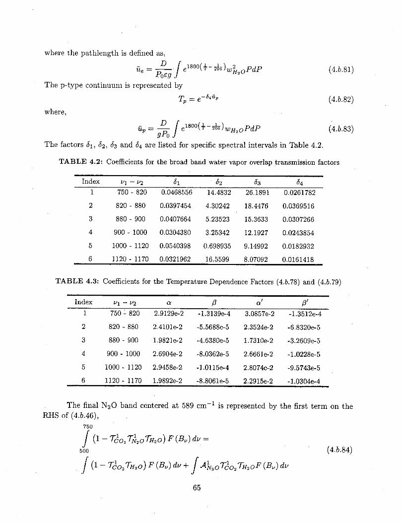
where the pathlength is defined as,
Pg Je1800( )w 2 oPdu- flsoo( 6 - H2 OPdP
The p-type continuum is represented by
Tp = e-64 p
where,
up= D J e8oo(-- 296) WH PdP
The factors 61, 62, 63 and 64 are listed for specific spectral intervals in Table 4.2.
(4.b.81)
(4.b.82)
(4.b.83)
TABLE 4.2: Coefficients for the broad band water vapor overlap transmission factors
Index
1
2
3
4
5
6
VI - V2
750 - 820
820 - 880
880 - 900
900 - 1000
1000 - 1120
1120 - 1170
Si
0.0468556
0.0397454
0.0407664
0.0304380
0.0540398
0.0321962
62
14.4832
4.30242
5.23523
3.25342
0.698935
16.5599
63
26.1891
18.4476
15.3633
12.1927
9.14992
8.07092
64
0.0261782
0.0369516
0.0307266
0.0243854
0.0182932
0.0161418
TABLE 4.3: Coefficients for the Temperature Dependence Factors (4.b.78) and (4.b.79)
Vl - V2
750 - 820 2.9129e-2
820 - 880 2.4101e-2
880 - 900 1.9821e-2
900 - 1000 2.6904e-2
1000 - 1120 2.9458e-2
1120 - 1170 1.9892e-2
The finalRHS of (4.b.46),
N 2 0 band centered at 589 cm- 1 is represented by the first term on the
750
J/ (1 - Te 2 T 2 oTH2 o) F (B) dv =
500
(1 - T o2 TH2 o) F (BV) dv + JAN20CO2 H 2 F (BV) dv
65
Index
1
2
3
4
5
6
-1.3139e-4
-5.5688e-5
-4.6380e-5
-8.0362e-5
-1.0115e-4
-8.8061e-5
a'
3.0857e-2
2.3524e-2
1.7310e-2
2.6661e-2
2.8074e-2
2.2915e-2
/'-1.3512e-4
-6.8320e-5
-3.2609e-5
-1.0228e-5
-9.5743e-5
-1.0304e-4
(4.b.84)
__
I _
- - --

where the last term in (4.b.84) represents the radiative effects of the 589 cm-l N 2 0 band,
A N2oTo 2T H 2oF (B,) dv - A1 ofoAo TH2oF (Bp) (4.b.85)
The absorptance for this band includes both the fundamental and hot band transitions,
A 2o = 2.65581 T ln{1+ U + u11 /---) (4.b.86)
[ A.n+/4 + u 1 (1 + 1/301) /4 + u (1 + 1/ ) J
where the pathlengths for this band can also be defined in terms of the 1285 cm-l1 bandpath length and mean lines parameters (4.b.63 - 4.b.66),
u= 0 .100090 3 (4.b.87)
and,
,8= 0.964282/3 (4.b.88)
and,
u1 = 0.0992746u3 (4.b.89)
and,
l3\ = 0.964282/3 (4.b.90)m- 1
The overlap effect of water vapor is given by the transmission factor for the 500 to 800cm-1 spectral region defined by Ramanathan and Downey (1986) in their Table A2. Thisexpression is thus consistent with the transmission factor for this spectral region employedfor the water vapor formulation of the first term on the right hand side of (4.b.84). Theoverlap factor due to the CO2 bands near 589 cm- is obtained from the formulation inKiehl and Briegleb (1991),
To 2 1+ = Uo2 (4.b.91)
+1 + 02 (o+l 2 )
where the functional form is obtained in the same manner as the transmission factor forCH4 was determined in (4.b.67). The 0.2 factor is empirically determined by comparing(4.b.91) with results from 5 cm - 1 Malkmus narrow band calculations. The pathlengthparameters are given by,
D 4.9411 x 10⁴ (1- e-960/T) 3 , dP~UCop 0 ---- = --- e- 9 6 0 /T (4.b.92)
and,
5.3228 P (4.b.93)C2+5xe 250300
66
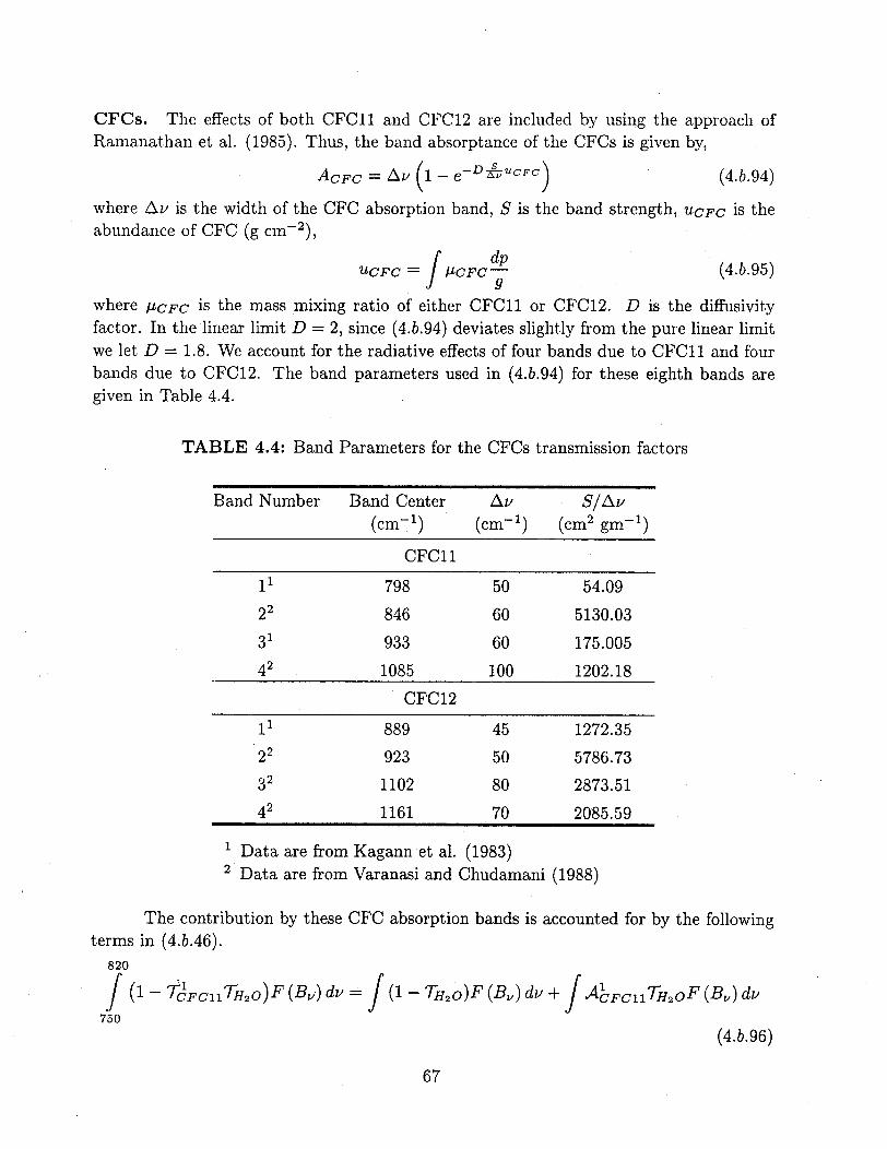
CFCs. The effects of both CFC11 and CFC12 are included by using the approach ofRamanathan et al. (1985). Thus, the band absorptance of the CFCs is given by,
ACFC = Av (- e-D ACFC) (4.b.94)
where Av is the width of the CFC absorption band, S is the band strength, UCFC is theabundance of CFC (g cm- 2 ),
UCFC =- CFC-dp9
(4.b.95)
where ICFC is the mass mixing ratio of either CFC11 or CFC12. D is the diffusivityfactor. In the linear limit D = 2, since (4.b.94) deviates slightly from the pure linear limitwe let D = 1.8. We account for the radiative effects of four bands due to CFC11 and fourbands due to CFC12. The band parameters used in (4.b.94) for these eighth bands aregiven in Table 4.4.
TABLE 4.4: Band Parameters for the CFCs transmission factors
Band Number Band Center Av S/Av(cm - ) (cm- 1) (cm 2 gm- 1)
CFC11
11 798 50 54.09
22 846 60 5130.03
31 933 60 175.005
42 1085 100 1202.18
CFC12
11 889 45 1272.35
22 923 50 5786.73
32 1102 80 2873.51
42 1161 70 2085.59
1
2Data areData are
from Kagann et al. (1983)from Varanasi and Chudamani (1988)
The contribution by these CFC absorption bands is accounted for by the followingterms in (4.b.46).
820
J (1 - TFllTo)F (B,) dv = (1- TH2 )F (Bv) dv + AFCll 2 oF (B , ) dv750
(4.b.96)
67

880
J (1 TCFCllTH2 )F (B) d = 1 TH2o)F (B) du +J CFC11H 2 oF (BV) dv820
(4.b.97)900
J (1 - FCl H 2o)F (BV) dv = (1 -THO)F (BV) dv + J ACFClF B dv880
(4.b.98)1000
J (1 C- 'CoH 2 TCFC1 FCFC12) F (BV) dv (1 TH2 0o)F (BV) dv+900
J CFC12TH2 F (BV) dv + J ACFC1 THOc2 OCF F (B) d+ (4.b.99)
faroTm o 2a 2, F (By ,AC02T H 2oTCFCllCFC12F (By)dv
1120
J (1 T- CO2To3 TH2OTC FClTFC2) F (B.) dv = J'(i - H 2 O)F ) d+1000
J AO3TH2OF (BV) dv+ (4.b.100)
3 4 3J A To2 3 H 2o7-CFC llCFCl2 F (BV) dv+
J ACFClTO3 TH2 OF (BV) dv + j AFCl2 T OF (BV) dv
For the 798 cm-1 CFC11 band, the absorption effect is given by the second termon the right hand side of (4.b.96),
ACFC11TH2oF (BV) dv" AFTF (B) (4.b.101)
where the band absorptance for the CFC is given by (4.b.94) and the overlap factor dueto water vapor is given by (4.b.74) using the index 1 factors from Tables 4.2 and 4.3.Similarly, the 846 cm-l CFC11 band is represented by the second term on the RHS of(4.b.97),
f A 2 FC 1TH F (B) dv MA2FC11TH2OF (BP) (4.b.102)
where the H 20 overlap factor is given by index 2 in tables 4.2 and 4.3. The 933 cm - 1
CFC11 band is given by the third term on the RHS of (4.b.99),
J ACFCT1 H2 oTFC 2F (BV) dv ACFC1TH2 oTFc F (B) (4.b.103)A~FC1THo FC H2CFC12 vc~
68

where the H 2 0 overlap factor is defined as index 4 in Tables 4.2 and 4.3, and the CFC12transmission factor is obtained from (4.b.94). The final CFC11 band centered at 1085cm-1 is represented by the fourth term on the RHS of (4.b.100),
ACFC11TO 3 oH2O F (By) dv AFclATo3 T F (Bo) (4.b.104)CA~FCll TO~3TH2 0 F (Bvd,,CFC11Ac 3 TH2os o
where the transmission due to the 9.6 micron ozone band is defined similar to (4.b.91) forCO2 as,
T3 = (4.b.105)i+C / ~u03
1+ E Uoi=1 4+Uo3(l+l
where the pathlengths are defined in Ramanathan and Dickinson (1979). The H 2 0 overlapfactor is defined by index 5 in Tables 4.2 and 4.3.
For the 889 cm-'1 CFC12 band the absorption is defined by the second term in
(4.b.98) as,
CFC12TH2, F (Bv) dv ACFC2TH2 F (B (4.b.106)
where the H 20 overlap factor is defined by index 3 of Tables 4.2 and 4.3, and the CFCabsorptance is given by (4.b.94). The 923 cm -1 CFC12 band is described by the secondterm in (4.b.99),
J ACFC1H 2OF (Bv) dv tAFC12TH2OF (Bo) (4.b.107)
where the H 2O overlap is defined as index 4 in Tables 4.2 and 4.3. The 1102 cm- 1 CFC12band is represented by the last term on the RHS of (4.b.100),
J ACFC12TO3 TH2 F (BV) dv -ACFCl 2TO 3TH 2oF (Bo) (4.b.102)
where the transmission by ozone is described by (4.b.105) and the H 2 0 overlap factoris represented by index 5 in tables 1 and 2. The final CFC12 band at 1161 cm- 1 isrepresented by the second term on the RHS of (4.b.69),
J ACFC12 H 2 F (B , ) dv ACFC12TH2 0F (Bo) (4.b.109)CFC127H2 CFC12TH2
where the H 20 overlap factor is defined as index 6 in Tables 4.2 and 4.3.
Minor CO 2 Bands. There are two minor bands of carbon dioxide that have been addedto the CCM longwave model. These bands play a minor role in the present day radiativebudget, but are very important for high levels of CO2, such as during the Archean. Thefirst band we consider is centered at 961 cm - 1. The radiative contribution of this band isrepresented by the last term in (4.b.99),
2I AO 2 TH2o FClTlFC2 F (B) dv AoTH2 OTFclF (Be) (4.b.110)/·C02 oTH20 llTCFC11 CFC12C0T2 F1F (B.) dv r, A 3 6FC1 F (Bo) (4.b.110)
69

where the transmission factors for water vapor, CFC11 and CFC12 are defined in theprevious section for the 900 to 1000 cm-1 spectral interval. The absorptance due to CO 2
is given by,
Ac 02 = 3.8443 1n 1 + (4.b.111)
where the pathlength parameters are defined as,
ul = 3.88984 x 10³ (Tp) we-1997-6/ T (4.b.112)
ul = 3.88984 x 10³ (Tp) we-1997.6/T (4.b.113)
U3 = 6.50642 x 10³c (Tp) we-2989-7 / T (4.b.114)
and the pressure parameter is,
/=3 2.97558 (P (4.b.115)
/2 = -p (4.b.116)
83 = 231 (4.b. 117)and,
(Tp (1- e-1360.0/Tp) 3
a{(Tp)= -- - (4.b.118)
The CO 2 band centered at 1064 cm-l is represented by the third term on the RHS of(4.b.100),
J ACo2 o 3 TH 2 oTO'TCFC11'CFC12F(Bv)d AC 2Ti03 TH 2 O TFCllT1 FClF(BP)
(4.b.119)where the transmission factors due to ozone, water vapor, CFC11 and CFC12 are definedin the previous section. The absorptance due to the 1064 cm-1 CO2 band is given by,
A = 3.8443 ln { 1 + Eu (} (4.b.120)
where the dimensionless pathlength is defined as,
ul = 3.42217 x 10³ a (Tp) we-1849.7/T (4.b.121)
u2 = 6.02454 x 10³ (Tp) we- 2782 l/T (4.b.122)
U3 = 5.53143 x 10³ a (Tp) we-3723.2/T (4.b.123)
where
(1- e- 1540./Tp) 3
a (Tp) - (4.b.124)VTP
70
The pressure factor, i01, for (4.b.120) is the same as defined in (4.b.115), while the otherfactors are,
P2 = 2P1 (4.b.125)
/3 = 32 (4.b.126)
In the above expressions, w is the column mass abundance of C02,dP IAC02
W = C0 2 P (4.b.127)9 9
where uco0 is the mass mixing ratio of CO 2 (assumed constant).
Mixing ratio of trace gases
The mixing ratios of methane, nitrous oxide, CFC11 and CFC12 are specified aszonally averaged quantities. The stratospheric mixing ratios of these various gases do varywith latitude. This is to mimic the effects of stratospheric circulation on these tracers.The exact latitude dependence of the mixing ratio scale height was based on informationfrom a two dimensional chemical model (S. Solomon, personal communication). In thetroposphere the gases are assumed to be well mixed,
ICH 4 = 0.55241wcH4 (4.b.128)
N 20 = 1.51913wN2 (4.b.129)
P/CFC11 = 4.69548WCFC11 (4.b.130)
]tCFC12 - 4.14307WCFC12 (4.b.131)
where w denotes the volume mixing ratio of these gases. The CCM3 employs volumemixing ratios for the year 1992 based on the 1994 IPCC report, WCH4 = 1.714 ppmv,WN20 = 0.311 ppmv, WCFCll = 0.280 ppbv and WCFC12 = 0.503 ppbv. The pressure level(mb) of the tropopause is defined as,
Ptrop = 250.0 - 150.0 cos2 q (4.b.126)
For p < Ptrop, the stratospheric mixing ratios are defined as,/ v \XCH4
1CH1 CH4 = C 4 ( (4.b. 133)Ptrop/
/ T \ ^XN 20
AN 2O = IN 20 ( Ptrop ) (4.b.134)
/ \XCFC11
~ICFC11 = -- CFC11 (rop (4.b.135)Ptropj
0 / \XCFC12
ItCFC12 = ICFC12 Pp) (4.b.136)XPtrop/
71

where the mixing ratio scale heights are defined as,
XCH4 = 0.2353XN 2 o = 0.3478 + 0.00116 [I /<45 (4.-137)7Qu < 45 (4.b.137)XCFC11 = 0.7273 + 0.00606 101
XCFC12 = 0.4000 + 0.00222 |[0and,
XCH4 - 0.2353 + 0.22549 ||XNo = 0.4000 + 0.01333 > 45 4.b.138)
XCFC11 = 1.0000 + 0.01333 1 1 45XCFC12 = 0.5000 + 0.02444 1||
where 0 is latitude in degrees.
Cloud emissivity
The cloud emissivity is accounted for by defining an effective cloud amount for eachmodel layer,
A'= ecdAc (4.b.139)
The cloud emissivity is defined as,
Ecld 1- e- D -absCWP (4.b.140)
where D is a diffusivity factor set to 1.66, Kabs is the longwave absorption coefficient(m 2g-1 ), and CWP is the cloud water path (gm- 2 ). The absorption coefficient is definedas,
Kabs = K (1 - fice) + Eiifice (4.b.141)
where 1I is the longwave absorption coefficient for liquid cloud water and has a value of0.090361, such that DKi is 0.15. ci is the absorption coefficient for ice clouds and is basedon a broad band fit to the emissivity given by Ebert and Curry's formulation,
1i = 0.005 + . (4.b.142)
Tre
Numerical algorithms
The downward longwave clear-sky flux at the surface is,
Fcr(Ps) = B(O)e(O,ps) + a (p'p dB (4.b.143)
while the upward flux at the surface is just
Ft(ps) = TBTS. (4.b.144)
72

The downward cloudy-sky flux at the surface is
F (ps) =-Fc$ (Ps)fclear + CT4 (plbk)A(Pc12)
~K IPs ~ dB (p') , ,,, (4.b.145)
+ EZ oT4(Pclbk) + a (Ps P ' ') dp' fcld (k) (k-=3 clbk ' p '
where Pclbk is the pressure level of the cloud base at k.
fcld(k) is the probability of a cloud existing in layer k, and clear sky below thislayer,
k-1
fcld(k) = A A(1 ) (4.b.146)i=2
orK
i (1-A)fcld(k) Ai=2 .(4.b.147)
i(1-AD)i=k
The clear-sky fraction for the total atmospheric column, fclear, is given byK
flear = (1 - Ai), (4.b.148)i=1
where AX is the fractional cloud cover in layer i and N is the total number of atmospheric
layers.
Fluxes within the atmosphere are evaluated at each interface (Figure 1) so that
longwave heating-rates are on model levels. The upward flux between the surface and the
lowest cloud layer is equal to the clear-sky upward flux,
FbtW(Pk) =Fclr(Pk). (4.b.149)
Within the layers that contain clouds, the upward flux isk.f
Fcld(k) = Fcr (Pk)fclear(k) + {aT4(pcitl)f=kjow (4.b.150)
["PkdB
- I (a(p',Pcltl)t) (P')dP' fld() Pk, < P < k < Pk+1,Y~cltl dpl
where fld(e) is the probability that a cloud is in layer £ and clear sky exists above layer £:K
k nH (1-A')fcld(£) = A J (1 - Ai) = A K+ (4.b.151)
i=e1 nH (1-AI)i=k+1
73

klo is the lowest level of cloud, kHI is the highest layer of cloud, and pcltl is the cloud-top level. The upward flux above the clouds is obtained from a similar expression. Thedownward flux above the cloudy region is equal to the clear-sky flux,
FbV(pk)= Fr (pk). (4.b.152)
Within the clouds and below the clouds, the downward flux isk H I
pk dBdbl(Pk) = Fi(Pk)fc d (k) + {OaT'(Pclbl) + c (p', }P
£=k Pclbl P (4.b.153)
X fCld(e), Ps < Pk < PHI,
where Pclbi is the cloud-base level, fcld(e) is the probability of a cloud existing in layer e
and clear sky below this level,K
e= n ( -AD)fcld(e) = A (1 -i A') = A -=k- (4.b.154)
=k H(1-A)i=£
The longwave atmospheric heating rate is obtained from
Q w(Pk) -g Ft(Pk+l) - F (Pk+l) - F(k) F k) (4.b.155)Cp Pk+1 - Pk
which is added to the nonlinear term (Q) in the thermodynamic equation.
The full calculation of longwave radiation (which includes heating rates as well asboundary fluxes) is computationally expensive. Therefore, modifications to the longwavescheme were developed to improve its efficiency for the diurnal framework. For illustration,consider the clear-sky fluxes defined in (4.b.34) and (4.b.35). Well over 90% of the longwavecomputational cost involves evaluating the absorptivity a and emissivity e. To reduce thiscomputational burden, pa and e are computed at a user defined frequency that is set toevery 12 model hours in the standard configuration, while longwave heating rates arecomputed at the diurnal cycle frequency of once every model hour.
Calculation of a and e with a period longer than the evaluation of the longwaveheating rates neglects the dependence of these quantities on variations in temperature,water vapor, and ozone. However, variations in radiative fluxes due to changes in cloudamount are fully accounted for at each radiation calculation, which is regarded to bethe dominant effect on diurnal time scales. The dominant effect on the heating rates ofchanges in temperature occurs through the Planck function and is accounted for with thismethod.
The continuous equations for the longwave calculations require a sophisticatedvertical finite-differencing scheme due to the integral term Sf adB in Equations (4.b.34)-
74

(4.b.35). The reason for the additional care in evaluating this integral arises from thenonlinear behavior of a across a given model layer. For example, if the flux at interface Pkis required, an integral of the form pk a(p' ,pk)dB(p') must be evaluated. For the nearestlayer to level Pk, the following terms will arise:
pk [a(Pk + (P, k)/ aW(p',pk)dB(p') =[( ,k)+ .(pk,Pk)] [B(pk) - B(k+)], (4.b.156)Pk+l
employing the trapezoidal rule. The problem arises with the second absorptivity a(pk, Pk),since this term is zero. It is also known that a is nearly exponential in form within a layer.Thus, to accurately account for the variation of a(p,p') across a layer, many more gridpoints are required than are available in CCM3. The nearest layer must, therefore, besubdivided and a must be evaluated across the subdivided layers. The algorithm that isemployed in is to use a trapezoid method for all layers except the nearest layer. For thenearest layer a subdivision, as illustrated in Figure 4, is employed.
For the upward flux, the nearest layer contribution to the integral is evaluated fromk+1
j/ adB(p') = a22 [B(p k l ) - B(pk)] + a21 [B(pk)- B(pk)], (4.b.157)
while for the downward flux, the integral is evaluated according tok
adB(p') = cll [B(pk) - B(pH)] + a 1 2 [B(pkH) - B(pk)]. (4.b.158)JPH
The aij, i = 1, 2; j = 1,2, are absorptivities evaluated for the subdivided pathsshown in Figure 4. The path-length dependence for the absorptivities arises from thedependence on the absorptance A(p,p') [e.g., Eq. (4.b.155)]. Temperatures are known atmodel levels. Temperatures at layer interfaces are determined through linear interpolationin logp between layer midpoint temperatures. Thus, B(pk) = OBTk' can be evaluated at allrequired levels. The most involved calculation arises from the evaluation of the fraction oflayers shown in Figure 3. In general, the absorptance of a layer can require the evaluationof the following path lengths:
S(PkPk+l) = f(T)pAp, (4.b.159)
and
u(pk, Pk+) = g(T)Ap, (4.b.160)
and
(3(pk,pk+l) =h(T)p, (4.b.161)
where f, g, and h are functions of temperature due to band parameters (see Kiehl andRamanathan, 1983), and T is an absorber mass-weighted mean temperature.
These pathlengths are used extensively in the evaluation of Ao3 (Ramanathan andDickinson, 1979) and ACO2 (Kiehl and Briegleb, 1991) and the trace gases. But path
75

22
21
a12
ET---^-
ll^ !r '__
k+1H
p k
kPH
Figure 3. Subdivision of model layers for radiation flux calculation
lengths dependent on both p2 (i.e., () and.p (i.e., u) are also needed in calculating thewater-vapor absorptivity, CaH 2o (Ramanathan and Downey, 1986). To account for thesubdivided layer, a fractional layer amount must be multiplied by 5 and u, e.g.,
11= (PHk+l ) UINPL(1, k) (4.b.162)
ill = u(p ,P 1+l ) x WINPL(1, k), (4.b.163)
and
P11 = (pH,pH+l) x PINPL(1, k), (4.b.164)
where UINPL, WINPL, and PINPL are factors to account for the fractional subdividedlayer amount. These quantities are derived for the case where the mixing ratio is assumedto be constant within a given layer (CO2 and H 2 0). For ozone, the mixing ratio is assumedto interpolate linearly in physical thickness; thus, another fractional layer amount ZINPLis required for evaluating Ao3 (p, p') across subdivided layers.
Consider the subdivided path for CO22; the total path length from pk to pk+1 forthe p2 path length will be
E(pH,p~H+) ) PH [PH - pH+] , (4.b.165)
where PH 2 PH+P . The total layer path length is, therefore, proportional to
, 2 2 H~((ppH+) ~((PH)2 _ (p+1)2 ). (4.b.166)
The path length ~ for CY22 requires the mean pressure
P22 {k ±P +P (4.b.167)2 I 2 2
76

and the pressure difference
pk+ p +lpAp22 + PH k (4.b.168)
Therefore, the path 622 is
622 P22 AP22 = ( PH+_) -(Pk1)2} (4.b.169)
The fractional path length is obtained by normalizing this by (pH, p '+),
UINPL(2, k)= DAF3(k) - (+l 1)2 (4.b.170)2(pH
where
DAF3(k) = (4.b.171)(p) 2 - 2
Similar reasoning leads to the following expressions for the remaining fractional pathlengths, for a21,
UINPL(3, k) DAF3(k) (P H - (k+ )2, (4.b.172)
for a1 1 ,
UINPL(1, k) = DAF3(k) {(p) 2 (P} (4. b.173)(k){( )i') (4.b.(173)
and for ca1 2 ,
UINPL(4, k) = DAF3(k) { (p) - p +r ) . (4.b.174)
The UINPL are fractional layer amounts for path length that scale as p2 , i.e., ij.
For variables that scale linearly in p, e.g., uij, the following fractional layer amountsare used:
WINPL(1, k) = DAF4(k) { P H 2 (4.b.175)
(rk k+1 l
WINPL(2, k) = DAF4(k) j42 H- j, (4.b.176)
2 J(4.b.177)WINPL(3.i, k) = DAF4(k) - P+ (4.b.177)
77

WINPL(4, k) = DAF4(k) {PH- ( 2 ) } (4.b.178)
where1
DAF4(k) = k + 1 ' (4.b.179)PH - PH
These fractional layer amounts are directly analogous to the UINPL, but since uis linear in p, the squared terms are not present.
The variable 3ij requires a mean pressure for the subdivided layer. These are
PINPL(1,Ik) = 2 { 2 + P} (4.b.180)
1 r7k±4 j1 kPINPL(2, k) + p 2 (4.b.181)2 2 " J
PINPL(3, k)= -{P +s pl (4.b.182)
1 lp+ +p I( + 182)PINPL(4, k) = p P +p . (4.b.183)
Finally, fractional layer amounts for ozone path lengths are needed, since ozone isinterpolated linearly in physical thickness. These are given by
ZINPL(1, k) = 2 ( f + P ' (4.b.184)
1i c \
ZINPL(2, k) = - , (4.b.185)
ZINPL(3, k) = ZINPL(1, k) + 2ZINPL(2, k), (4.b.186)
ZINPL(4, k) = ZINPL(2, k) + 2ZINPL(1, k). (4.b.187)
78

c. Surface Exchange Formulations
The surface exchange of heat, moisture and momentum between the atmosphereand land, ocean or ice surfaces are treated with a bulk exchange formulation. We presenta description of each surface exchange separately. Although the functional forms ofthe exchange relations are identical, we present the descriptions of these componentsas developed and represented in the various subroutines in CCM3. The differences inthe exchange expressions are predominantly in the definition of roughness lengths andexchange coefficients. The description of surface exchange over ocean and sea ice followsfrom Bryan et al. 1996
Land
Land surface fluxes of momentum, sensible heat, and latent heat are calculatedfrom Monin-Obukhov similarity theory applied to the surface (i.e., constant flux) layer.The zonal re and meridional ry momentum fluxes (kg m-l s -2) are
= - (u-P1 s) (4.c.1)ram
Ty --P1 (4.c.2)ram
where pi, ul, and vl are the density (kg m- 3 ), zonal wind (m s-1), and meridional wind(m s-1 ) at the lowest model level. By definition, the surface winds Us and v, equal zero.ram is the aerodynamic resistance (s m- 1) for momentum between the lowest model levelat height zl and the surface at height ZOm + d, where ZOm is the roughness length (m) formomentum and d is the displacement height (m)
ra = k2 VI1 [In ( 1- d) bm(C)] [ln (zl-d)_ - bm()] (4.c.3)m kV11 , ZOM Zorm
where k = 0.4 is the von Karman constant and IVi = v/u + v. Atmospheric stabilityZ1 -d
is defined by C = . The length scale L (m) isL
3
L = (4 .c. 4 )X 9 H+0.61cp T E
k TvlV Plcp
79

where u, is the friction velocity (m s- 1), g is gravitational acceleration (m s-2), TV1 is thevirtual temperature of the lowest model level (K), H is the sensible heat flux (W m- 2 ), cpis the heat capacity of air (J kg-1 K-1), T1 is the temperature of the lowest model level(K), and E is the water vapor flux (kg m-2 s-l). The term 0.61cp T1 E accounts for thebuoyancy effects of water vapor. 21 'm is a function that increases this resistance for stableconditions (( > 0) and decreases this resistance for unstable conditions (( < 0)
mm()- -5C for C>0 (4.c.5)
forQ <0 (4.c.6)) =21n) + In )- 2tan-lx + 2 for < 0 (4..6)
where x = (1 - 16C)1/4
The sensible and latent heat fluxes are calculated in a manner analogous to themomentum fluxes, but are complicated by the need to partition these fluxes into groundand vegetation components. Land surface fluxes of sensible heat and latent heat arecalculated by finding the vegetation T, and ground Tg temperatures (K) that balance thevegetation and ground energy budgets
-~v + ' v + Hv + A Ev- 0 (4.c.7)
- + g+ Hg+ Eg +G= (4.c.8)
where , is the absorbed solar radiation (W m- 2 ), L is the absorbed longwave radiation(W m- 2 ), H is the sensible heat flux (W m-2 ), AE is the latent heat flux (W m- 2 ),G is the soil heat flux (W m- 2 ), and the subscripts "v" and "g" indicated vegetationand ground, respectively. The solar radiation absorbed by the vegetation and the grounddepends on the amount of leaf and stem material present (i.e., the leaf and stem areas),their optical properties, and the optical properties of snow and soil. The other terms inthese two equations depend on the vegetation and ground temperatures, which are foundthrough Newton-Raphson iteration. The soil heat flux is then used to melt snow, if theconditions are right, and to update soil temperatures for a six-layer soil column using aheat diffusion equation that accounts for phase change. The latent heat fluxes are usedto update vegetation, snow, and soil water pools. Soilwater is calculated for the six-layer column using a one-dimensional conservation equation that accounts for infiltration
80

input, gravitational drainage at the bottom of the column, evapotranspirational losses,and vertical water flow based on lead gradients.
The vegetation and ground sensible heat fluxes are
Hv = -picp(T, - Tv)chv (4.c.9)
Hg = -piCp(Ts - Tg)chg (4.c.10)
where Ts is the "surface" temperature (K). Chv is a vegetation conductance (m s - )
that depends on leaf and stem area and the wind within the canopy. chg is a groundconductance that depends on turbulent transfer processes within the vegetation canopy.The surface temperature Ts is eliminated from these equations by assuming the canopyair has negligible capacity to store heat so that the total sensible heat flux between thesurface and the atmosphere is
(O1 -T)TSH = -plCp s) = Hv + Hg (4.c.11)rah
where 01 is the potential temperature (K) at the lowest model level and rah is anaerodynamic resistance (s m - 1) for sensible heat.
Similarly, the vegetation and ground latent heat fluxes are
AEV = PlP [es - e,(Tv)](cwe + cwt) (4.c.12)7
AEg =- p [e, - e, (Tg)]cwg (4.c.13)
where y is the psychrometric constant (Pa K- 1), e, is the vapor pressure (Pa) at thesurface, and e*(Tv) and e*(Tg) are the saturation vapor pressures (Pa) evaluated at thevegetation and ground temperatures. Cwe is a vegetation conductance for evaporation ofintercepted water. It depends on leaf and stem area, the fraction of the canopy that iswet, and the wind within the canopy. Water is lost from the soil as transpiration fromthe non-wetted fraction of the canopy with a conductance ct that depends on leaf area,the wind within the canopy, and stomatal responses to light, temperature, soil water,vapor pressure, and CO2 concentration. cwg is a ground conductance for evaporation of
81

soil water, which decreases as the soil becomes drier. The surface vapor pressure e, iseliminated from these equations by assuming negligible capacity to store water vapor sothat the total latent heat flux between the surface and the atmosphere is
AE = P1 P (e - e) = AE, + AEg (4.c.14)Y raw
where e1 is the vapor pressure (Pa) at the lowest model level and raw is an aerodynamicresistance (s m - 1) for water vapor.
The resistances rah and raw are analogous to the aerodynamic resistance formomentum
rah = k2Vll [n (Zl ) - m() [ln ( l- d) -h()] (4.c.15)
raw-[n K - r [ - d -' Z- I' ((\1r a w = k2IVl \ln( z- d )- (C)] [inn Om) -i,()] (4.c.16)
where ZOh and zow are the roughness lengths (m) for sensible and latent heat. OIh, and Oware functions, similar to Okm, that increase these resistances for stable conditions (C > 0)and decrease thse resistances for unstable conditions (C < 0)
Oh(0) = Ow(C) = -5( for C > 0 (4.c.17)
Ph (C) = Vw(C =)z 21n + 2) for ( < O (4.c.18)
where x = (1 - 16)1/4
In addition to the momentum, sensible heat, and latent heat fluxes, landsurface albedos and upward longwave radiation are needed for the atmospheric radiationcalculations. Surface albedos depend on the solar zenith angle, the amount of leaf andstem material present, their optical properties, and the optical properties of snow andsoil. The upward longwave radiation is the difference between the incident and absorbedfluxes.
82

These and other aspects of the land surface fluxes have been described by Bonan(1996a).
Ocean and sea ice
The bulk formulae used for the ocean-atmosphere or sea ice-atmosphere exchangeare:
T = pACDII\UII\AU
E = pACDlI\UllIAq (4.c.19)
H = pACpCHIIAUIIAwhere PA is atmospheric surface density, and Cp is the specific heat.
The transfer coefficients between ocean and atmosphere (i = ocn) or sea-ice andatmosphere (i = si), shifted to a height, ZA,and to the stability, (i, appropriate to theparticular interface, are:
CD 2 [n (z O ) - m
CEi = K2 [in ( ) - m] ' [in (z)- s]
CHi = -2 [In (Z- ) I-m] j [n (/zh) - S]
where n = 0.4 is von Karman's constant and the integrated flux profiles, ibm formomentum and 4s for scalars, are functions of the stability parameter, (i. These functionsas used in the model are:
m (C) = s(0) = -5C > 0
m() = 21n[0.5(l + X)] + ln[0.5( + X 2)] - 2 tan- l X + 0.57r < 0
S(() = 21n[0.5(1+X 2)] ¢ < 0
X = (1 - 16)1/4
The stability parameter is,
= Kg 9 ZAZ (0- Q Itu i 2 v ,+ (Zv- 1 +qA)
where virtual potential temperature is computed as OV = A (1 + ZqA), Qo and OA arethe lowest level atmospheric humidity, and potential temperature, respectively, and Zv(e(water)/g(air)) - 1 = 0.606. Since Ci is itself a function of the turbulent scales andhence the fluxes, an iterative procedure is generally required to solve (4.c.19). And where
83

the turbulent velocity scales are given by
u~-= CDD'/ 2 la l
Q*= CE IA lJI (Aiq) u- 1 (4.c.20)
;= CHi |AUil (A0i) u - 1,
For the ocean interface (i = ocn),
AU Uo
Aq = qo - 0.98p -C 5 exp(C6/Ts)
AO 0o - T,
where the factor 0.98 accounts for the salinity of the ocean,C5 = 640380 kg m- 3 and C6=-5107.4 K.
The roughness length for momentum, Zo,, in meters, is a function of theatmospheric wind at 10 meters height, U1o:
0 C1Zon = 10exp- K -( +C2 + CUo
where C1 = 0.0027 m/s, C2 = 0.000142, and C3 = 0.0000764 m-is. The correspondingdrag coefficient at 10m height and neutral stability is
C0 = C 1 Uio + C2 + C3 U1 0
The roughness length for heat, Z^h, is a function of stability, and for evaporation, Zo,is a different constant:
Z =2.2 x 10⁻⁹ m 3> 0
= 4.9 x 10⁻⁵m 3 < 0Zocn= 9.5 x 10- 5 m.
Since the roughness lengths are neither constant nor equal, the iterative solutionfor the fluxes (4.c.19)is as follows: first, (cn is set incrementally greater than zero whenthe air-sea temperature difference suggests stable stratification, otherwise it is set to zero.In either case, Om O = = S 0, and the initial transfer coefficients are then found fromthe roughness lengths at this ,ocn and Ulo = UA. As with sea-ice, these coefficients areused to approximate the initial flux scales (4.c.20) and the first iteration begins with anupdated Con and calculations of rm and Usb. The wind speed, UA, is then shifted to itsequivalent neutral value at 10m height :
10U -o=UA (1 + i ln( - c))) .
This wind speed is used to update the transfer coefficients and hence the flux scales. Thesecond and final iteration begins with another update of (ocn. The final flux scales thengive the fluxes calculated by (4.c.19).
84

The state variables required to calculate the fluxes over sea ice (i - si) (4.c.19)are the atmospheric wind velocity, potential temperature, density and specific humidity in(kg/kg) at a height ZA, and the ice surface temperature Tsi.
AU-Uo
Aq = qopA1 C 5exp(C 6/Ti)
A9 = 'o - Tsi
Presently the coupler assumes constant and equal roughness lengths for ice :
Z Z Z = Z = 0.04m.
To start the iterative solver for the fluxes (4.c.19), (si is set to zero : Am = Is = 0,and the neutral coefficients are used to approximate the flux scales (4.c.20). The iterationbegins by computing (Si, finding the non-neutral transfer coefficients and updating theflux scales. After two such iterations there is sufficient convergence to compute the fluxes
(4.c.19).
d. Vertical Diffusion and Atmospheric Boundary Layer Processes
Local diffusion scheme
An explicit, non-local Atmospheric Boundary Layer (ABL) parameterizationis incorporated into the vertical diffusion parameterization in CCM3. The ABLparameterization includes a determination of the boundary layer depth. Above the topof the ABL, CCM3 employs a standard local diffusion parameterization for the freeatmosphere. In practice, the free atmosphere diffusivities are calculated first at all levels.The ABL scheme then determines the ABL depth and diffusivities and replaces thefree atmosphere values for all levels within the ABL. The implementation of the ABLparameterization in CCM is discussed in Holtslag and Boville (1993), while the formalismonly is discussed here.
The local form of the vertical diffusion terms of momentum, sensible heat, andmoisture follows those described by Smagorinsky et al. (1965) and Manabe et al. (1965)where the tendencies are given by
9u 1 r-\ 9 -rxAUOt 1ŽŽ =gh a (4.d.1)at p z Op
9v 1 9r, 9r9t s sl -9 '(4.d. 2)at p az 9 p '(4.d.2)
A0 1 AH g aOH(4.d.3)
9t pCp OZ Cp 9p '
85

aq 1 OR ORA -p =g -ap. (4.d.4)t= ~ppOz Op
Above the surface layer, the upward fluxes of momentum, sensible heat, and moisture dueto turbulent motions are given by
7rA pw'U = -pKm gKc (4.d.5)
r7,= pw'Vl- = gp2Kc p -, (4.d.6)O0z Op
H = pw' ' =-cppKe = Cpgp2K , (4.d.7)
,q aqR = pwq =-pKq = gp2K , (4.d.8)
where 0 = T P* and p* is a reference pressure which in practice is taken to be p,.
The variables Kc, where c E (q, 0, u, v) are "eddy-diffusivities" that are typically takenas functions of length scales £c and local vertical gradients of wind and virtual potentialtemperature, e.g.,
Kc = £C2SFc(Ri). (4.d.9)
Here S is the local shear, defined by
VS= (4.d.10)
and the mixing length ec is generally given by1 I 11 _1 1z (4.d.11)
£c kz AC'where k is the Von Karman constant, and Ac is the so-called asymptotic length scale,taken to be 30 m above the ABL. Since the lowest model level is always greater than 30 min depth, ic is simply set to 30 m in CCM3. Furthermore, Fc(Ri) denotes a functionaldependence of Kc on the gradient Richardson number:
Ri = g 0/Oz (4.d.12)i= S 2
where 0, is the virtual potential temperature,
=0 ( + R I (4.d.13)
For simplicity, in our present implementation of the local K approach, we specifythe same stability functions Fc for all c. For unstable conditions (Ri < 0) we choose
F,(Ri) = (1 - 18Ri)/ 2, (4.d.14)
86

and we use (4.c.12) for stable conditions (Ri > 0). This means that no distinction is madebetween vertical diffusion of heat, scalars and momentum.
"Non-local" atmospheric boundary layer scheme
In a local diffusion approach, the turbulent flux of a quantity is proportional tothe local gradient of that quantity (e.g., (4.d.5)-(4.d.8)). In such an approach the eddydiffusivity depends on local gradients of mean wind and mean virtual temperature (see(4.d.9)). These are reasonable assumptions when the length scale of the largest turbulenteddies is smaller than the size of the domain over which the turbulence extends. In theAtmospheric Boundary Layer (ABL) this is typically true for neutral and stable conditionsonly. For unstable and convective conditions, however, the largest transporting eddies mayhave a similar size as the boundary layer height itself, and the flux can be counter to thelocal gradient (Deardorff, 1972; Holtslag and Moeng, 1991). In such conditions a localdiffusion approach is no longer appropriate, and the eddy diffusivity is better representedwith turbulent properties characteristic of the ABL. We will refer to such an approach asnon-local diffusion.
To account for "non-local" transport by convective turbulence in the ABL, the localdiffusion term for constituent c is modified as
wC' =-Kc( - ) (4.d.15)Oz /
where Kc is the non-local eddy diffusivity for the quantity of interest. The term -cis a "non-local" transport term and reflects non-local transport due to dry convection.Eq. (4.d.15) applies to potential temperature, water vapor, and passive scalars. Nocountergradient term is applied to the wind components, so (4.d.1) and (4.d.2) remainunchanged. For stable and neutral conditions the non-local term is not relevant forany of the quantities. The eddy diffusivity formalism is, however, modified for unstableconditions.
In the non-local diffusion scheme the eddy diffusivity is given by
Kc = k (1 - (4.d.16)
where wt is a turbulent velocity scale and h is the boundary layer height. Equation (4.d.16)applies for heat, water vapor and passive scalars. The eddy diffusivity of momentum Kin,is also defined as (4.d.16) but with wt replaced by another velocity scale win. With properformulation of wt (or w,) and h, it can be shown that equation (4.d.16) behaves well fromvery stable to very unstable conditions in horizontally homogeneous and quasi-stationaryconditions. For unstable conditions wt and w, are proportional to the so-called convectivevelocity scale w*, while for neutral and stable conditions wt and Wm are proportional tothe friction velocity u,.
87

The major advantage of the present approach over the local eddy diffusivityapproach is that large eddy transport in the ABL is accounted for and entrainment effectsare treated implicitly. Above the ABL, 7c = 0 so (4.d.15) reduces to a local form with Kcgiven by (4.d.9). Near the top of the ABL we use the maximum of the values by (4.d.9)and (4.d.16), although (4.d.16) almost always gives the larger value in practice.
The non-local transport term in (4.d.15), cy, represents non-local influences on themixing by turbulence (Deardorff, 1972). As such, this term is small in stable conditions,and is therefore neglected under these conditions. For unstable conditions, however, mostheat and moisture transport is achieved by turbulent eddies with sizes on the order ofthe depth h of the ABL. In such cases, a formulation for yc consistent with the eddyformulation of (4.d.15) is given by
yca = W a (4.:d.17)Wm2h
where a is a constant and (w'C'), is the surface flux (in kinematic units) of the transportedscalar. The form of (4.d.17) is similar to the one proposed in Holtslag and Moeng (1991).The non-local correction vanishes under neutral conditions, for which w, = 0.
The formulations of the eddy-diffusivity and the non-local terms are dependent onthe boundary layer height h. The CCM2 configuration of this non-local scheme made useof a traditional approach to estimating the boundary layer depth by assuming a constantvalue for the bulk Richardson number across the boundary layer depth so that h wasiteratively determined using
Ri, {u((h)2 + (h)2)}9 - (4.d.18)9(g/0) (Ov(h) - '8)
where Ricr is a critical bulk Richardson number for the ABL; u(h) and v(h) are thehorizontal velocity components at h; g/Os is the buoyancy parameter and 0v(h) is thevirtual temperature at h. The quantity Os is a measure of the surface air temperature,which under unstable conditions was given by
s = O (Zs) + b (w )S, (4.d.19)Wm
where b is a constant, (w'0)s, is the virtual heat flux at the surface, O (z 8) is a virtualtemperature in the atmospheric surface layer (nominally 10 m), b (w'O),s/Wm represents atemperature excess (a measure of the strength of convective thermals in the lower part ofthe ABL) and unstable conditions are determined by (w''),s > O. The quantity ,v (z,) wascalculated from the temperature and moisture of the first model level and of the surfaceby applying the procedure in Geleyn (1988). The value of the critical bulk Richardsonnumber Ricr in (4.d.18), which generally depends on the vertical resolution of the model,was chosen as Ricr = 0.5 for the CCM2.
88

Vogelezang and Holtslag (1996) have recently studied the suitability of thisformulation in the context of field observations, large-eddy simulations (Moeng andSullivan, 1994), and an E- e turbulence closure model (Duynkerke, 1988). Theypropose a revised formulation which combines shear production in the outer region ofthe boundary layer with surface friction, where the Richardson number estimate is basedon the differences in wind and virtual temperature between the top of the ABL and a lowerheight that is well outside the surface layer (i.e., 20 m - 80 m). In addition to providingmore realistic estimates of boundary layer depth, the revised formulation provides asmoother transition between stable and neutral boundary layers. Consequently, CCM3employs the Vogelezang and Holtslag (1996) formulation for estimating the atmosphericboundary layer height, which can be written as
Ricr (u(h) - USL)2 + (v(h) - VSL) 2 + 3u2
h = z+ (/sL) ((- L) (4.d.19.1)(g/1sL) (Os(h)- OSL)
The quantities USL, VSL, and OSL represent the horizontal wind components and virtualpotential temperature just above the surface layer (nominally O.lh). In practice, thelowest model level values for these quantities are used to iteratively determine h forall stability conditions, where the critical Richardson number, Ricr, is assumed to be0.3. The disposable parameter B has been experimentally determined to be equal to100 (see Vogelezang and Holtslag, 1996). The computation starts by calculating the bulkRichardson number Ri between the level of OSL and subsequent higher levels of the model.Once Ri exceeds the critical value, the value of h is derived by linear interpolation betweenthe level with Ri > Ricr and the level below.
Using the calculated value for h and the surface fluxes, we calculate the velocityscales, the eddy diffusivities with (4.d.16), and the countergradient terms with (4.d.17),for each of the transported constituents. Subsequently, the new profiles for 0, q, u, and vare calculated using an implicit diffusion formulation.
The turbulent velocity scale of (4.d.16) depends primarily on the relative height z/h(h is boundary layer height), and the stability within the ABL. Here stability is definedwith respect to the surface virtual heat flux (w'0)s,. Secondly, the velocity scales arealso generally dependent on the specific quantity of interest. We will assume that thevelocity scales for mixing of passive scalars and specific humidity are equal to the onefor heat, denoted by wt. For the wind components, the velocity scale is different anddenoted by wn. The specification of wt and wm is given in detail by Troen and Mahrt(1986). Holtslag et al., (1990) have rewritten the velocity scale, in terms of the morewidely accepted profile functions of Dyer (1974), and have given a new formulation forvery stable conditions. Below we follow the latter approach.
89

For stable ((w'' )s < 0) and neutral surface conditions ((w' )s- = 0), the velocityscale for scalar transport is
Wt = u - (4.d.21)Oh
where u, is the friction velocity defined by
u* = [(u'') + ( vw') 2 ] 1 /4 (4.d.22)
Furthermore, Oh is the dimensionless vertical temperature gradient given by (Dyer, 1974),Z
;h= 1 + 5, (4.d.23)
for 0 < z/L < 1. Here L is the Obukhov length, defined by3
L - -u*3K^ ' ·L= (4.d.24)k(g/Ovo)(w''0)o
For z/L > 1,
h = 5 + L ' (4.d.25)
which matches (4.d.23) for z/L = 1. Equation (4.d.25) is a simple means to prevent Oh
from becoming too large (and K, too small) in very stable conditions. In stable conditions,the exchange coefficients for heat and momentum are often found to be similar. Thereforewe may use Wm=Wt.
For unstable conditions (w'0')s > 0, we have that wt and Wm differ in the surfacelayer (z/h < 0.1) and in the outer layer of the ABL (z/h > 0.1). For the surface layer, wtis given by (4.d.21) with
/bh - z)- 1 / 2
'h = (i - 15y) . (4.d.26)\ L L /Similarly, Wm is written as
,.Wm.= O , (4.d.27)
Wm
where ')m is the dimensionless wind gradient given by
/m (- z \- 1/ 3
'Pm = (- 15) . (4.d.28)
In the surface layer, the scalar flux is normally given by
('c')o= -. (4.d.29)Oh k 9Z/
Comparison with (4.d.15) and (4.d.16) shows that, in the surface layer, we should havea = 0 in (4.d.17) for consistency.
For the outer layer, wt and Wm are given by
Wt = Wm/Pr, (4.d.30)
90

where
Wm = (U* + CW ,) (4.d.31)
and
w = ((glOvo) (w'O)oh) /3 (4.d.32)
is the convective velocity scale. Furthermore, Pr is the turbulent Prandtl number andcl is a constant. The latter is obtained by evaluating the dimensionless vertical windgradient qOm by (4.d.28) at the top of the surface layer, as discussed by Troen and Mahrt(1986). This results in c1 = 0.6. For very unstable conditions (h > -L or w*/u* > 0),it can be shown with (4.d.30) that Wm is proportional to 0.85 w,, while for the neutralcase Wm = u*. The turbulent Prandtl number Pr (= Km/Kh = Wm/t) of (4.d.30) is
evaluated from
Pr = ( + akz- W* (4.d.33)Om L hwm
for z = O.lh. Equation (4.d.33) arises from matching (4.d.15), (4.d.16), (4.d.17), and(4.d.29) at the top of the surface layer. As in Troen and Mahrt we assume that Pr isindependent of height in the unstable outer layer. Its value decreases from Pr = 1 forthe neutral case (z/L = 0 and w* = 0), to Pr = 0.6 for w*/u*, _ 10 in very unstableconditions.
In very unstable conditions, the countergradient term of (4.d.17) approaches
wCo7c = d (4.d.34)
where d ^ a/0.852, because for very unstable conditions we obtain Wm ^ 0.85w*. Sincetypically d - 10 (Troen and Mahrt 1986), we have a = 7.2. Similarly, the temperatureexcess of (4.d.19) reads in this limit as d(w' O,)o/w*. This leads to b (= 0.85 d) = 8.5 in(4.d.19).
Finally, using the velocity scales described above, the flux equation (4.d.15) iscontinuous in relative height (z/h) and in the boundary layer stability parameter (h/Lor w*/u*).
In summary, the vertical diffusion tendency is given by the vertical derivative ofthe turbulent flux defined in (4.d.15):
0C 10 [-~ ==--- lpw'C/J
At p 9z [P(i
-=pz [PKc(z Y7c)] (4.d.35)
The vertical diffusion is implemented using a time-split implicit method. Thecountergradient term in the non-local ABL scheme depends on the surface flux,the boundary layer depth and the velocity scale, but not explicitly on the diffused
91

quantity. Therefore the countergradient term cannot be treated implicitly. Forward timedifferencing is used for the diffusion, whereas a leap frog (centered) method is used for thedynamics. Thus, the diffusive forward step is over two time steps. The time discretizationthen results in:
-2t- p Kc _~_^ )\ (4.d.36)2At -p n 6 - 1 (4.d.36) z [O
where subscripts n - 1 and n +1 refer to time levels, with Kcn-1 and -y-1 evaluated usingmodel variables at time n - 1. The whole diffusion process is time split from all otherprocesses so that time n - 1 variables may already have contributions from the dynamicsand other physical process. Equation (4.d.36) can be rewritten as
Cn+l = (1 - 2tGn-i)- lC*, (4.d.37)
C* = Cn-1 - 2AtHn-1(7 n -1), (4.d.38)
where G and H are differential operators. There can be a problem in applying (4.d.38) fortrace constituents, including water vapor, because these quantities are positive definite.The application of the countergradient term, H n - l(y n - l) may result in negative valuesfor C*, which are not removed by the subsequent implicit diffusion step. This problemis not strictly numerical; it arises under highly non-stationary conditions for which theABL formulation is not strictly applicable. In practice, we evaluate C* and check fornegative values in the constituent profiles. If a negative value is found, we set C*Cn-1 for that constituent profile (but not for other constituents at the same point). Notethat (4.d.37) is just the normal diffusion equation, which is solved using the numericaltechniques discussed in the next sub-section.
Numerical solution of nonlinear, time-split'vertical diffusion
As described in section 2, the vertical diffusion is calculated prior to the maindynamical calculation. This time-split diffusion is
n+ _n+ln+i n-i TAk+i/2 Ak--1/2Un = u-1 + 2At Pc kA -/ 2 (4.d.39)
PkLZkHn+l _n+l
+k = O + 2t k+i/2 _k-i/2 (4.d.40)
HnD+ l ._ n+lcpk pklz_
Rn+i HRn+iOn+1 _On-i 4 9 k+1/2 k-1/2
q n+l n-1- + 2A t k+l/2 k-1/2qk =qk + n-i
Pk- LZk
92
The surface fluxes are given by the explicit forms (4.d.5)-(4.d.8):
Rn+l = RK = LP (w'q') (4.d.44)
K+1/2 = HK+1/ = CPP1 (wO) (4.d.45)K+i/2 K+1/2 sCpPl s'
n+I __ n-1 (4.d.46_AK+1/2 = XTK+1/2 = P1 (u) (4.
+1/2 = T41/ 2 P1 (W v'). (4.d.47)%K+1/2 AK+1/2 Pi (W'7').
Note that these surface fluxes are explicit and ensure conservation of energy and moisturein the surface exchange. The surface stresses rT and r, could be made implicit withoutaffecting this conservation. In the free atmosphere, for k =1 to K - 1,
"n+l n+1n+l _ fn-1 K n-l +1 k
TAk+l/2 = ( /) Kk+1 /2 u - u Xj (4.d.48)' R Tk+l/ k+1/2 k+ /2 n-1 n- -..Zk+l k
n+ 1 - n+ink+i / f,-1 K -- l +1 (4.d.49)
Tkc+1/2 k+1/2 k+1/2 n-1 n-1 'Zk+l - Zk
n+1 n+lRn+1 ( ^n-1 K n--l kc- qk (4.d.50)
k+1/2 - -P k/2)2 (4.d.5)n-1'P,~k1/2 k/ In-i- n-- ik/ - 1Zk + l -- Zk
rR+l C l + n-1 Kn 1 "k+1 (4.d.51)-- k+1CPk'- P+1/2 4k+1/2 k+/2 n-1 n-1' .. 1
Kk'l is then determined from the neutral K modulated by a function of Richardson
++1 2
number
Kk+1/ = (KfN )k+l/ 2 * f(RIk+l/ 2 ) (4.d.54)
p2 n-1.n-1 ^____________^Pk+l/2
with a minimum value for KJ~l1 2 of Kmin = 0.01.
f max (0,1 - Ri/Ric) for RI > O (stable) ,fp-1)2 (RI__ =1 + Rvn1(4.d.55)
/1 - 18RI for RI < O (unstable) ,
with a critical Richardson number at which f goes to zero of
RIC=0.2 . (4.d.56)R c= 0.2 (.d.
93

The neutral KN is calculated by
n-1 l ) 1 2 (Vn-1 n-1 ) 2] 1/ ( .5(K~-rv-)l/ 2 = £ ~ L\U~+1/2[ - U- V1 - -1(KW"I~+1/2 k+1/2---- . -- - (4.d.57)
ck+l/2
with
-1 n - l - n-1 n-1 (i C59)zk+1/2 = k+1 - (4d.59)
and £k+1/2 is determined from (4.d.11) and (4.d.13). The Richardson number in the freeatmosphere is calculated from
2g (z k -·1 n-1= 2g (4 - iR _ ^9 \nk _4Zk+l
Ik +1/2 ( n-l + nn-l -1(Oiv + c+)
(4.d.60)n-1i_ - n-1
^X V________k ~ 1Vk+l(Un- 1 ,n-l 2 , / n-1 n-l 2
L k+1 - Uk ) + Vk+1 - vk
where
0 k -= ok-1 1.0 + R 1) ) (4.d.60.1)
Within the diagnosed atmospheric boundary layer, the diffusivities are modified by thenon-local atmospheric boundary layer scheme described earlier. At the top of the model,the fluxes are set to 0,
X1/2 - "~ 1/2"i/2 1/2TA1/2 = T41/2 = R1/2 = H1 = 0. (4.d.61)
The diffusion equations can be summarized as
_n+ 1 ^ L -1 - n n) n (4k -{ } k(u -aCk (+Uk -- u+), (4.d.62)
k+ l - {V-l}k - ak (k+1 - v ) -Ck (vk+ - Vk 1 ) (4.d.63)
qk+ - {qI- 1} ak (qk+l -_ ) - Ck (qk_ 1 -q 1)+ (4.d.64)
on+l - {OnL}k ak [Oi+ 1 - 9+ 1l] - Ck [rn+i - l,] (4.d.65)
for 1 < k < K - 1,
{U- }k = - 1i (4.d.66)
{ V }n k 1Vk (4.d.67)
{fq- 1 =} q - 1 (4.d.68)
{0n-o1 k = - , (4.d.69)
94
and for k = K,
U -}KUK 2 At n-n+l1
Vn- K = Un- + nt
V-xK-K P+n ~+/PK+½AZK-l 1/2
V n-1 _= Vn-1 2At n+{ 1 -}K- K + Azn-l K+1/2 '
{qn-} K- qK +
{n-1K = e-1 +
2At Rnl
2At
PK+1AZK 1 K+1/2
Wrn+l
CK PK+ Az- "'L K+1/2 '
2Atak = APk (Pk+ 1 - Pk)
pn-1 )2g k+l/2 -n-i Ps 1 ck+ l /2p-
1<k<K-1,
aK = 0,
C1 = 0,
2 (pAt 1) 1/ ) K -t n-1 n ((-n2-i nn-i
A (p Pk-1)K2 < K.
The left-hand side of (4.d.65) can be written in terms of T because it is represented as adifference.
Following Richtmeyer and Morton (1967, pp. 198-201), the solutions for u, v,0,and q have the form,
Uk l -= Fuk + Eku'+l, (4.d.78)
where for k = 1,
{ n-- }1Fu- =
bl
gaEl - a,bl
(4.d.79)
(4.d.80)
and for 2 < k < K - 1,
{un-}k + CkFUk-1FUk = Cbkk--k-
bk - CkEk-l(4.d.81)
95
(4.d.70)
(4.d.71)
where
(4.d.72)
(4.d.73)
(4.d.74)
(4.d.75)
(4.d.76)
(4.d.77)
Ek = -ak (4.d.82)bk -CkEk-1
and for k = K,
EK = 0, (4.d.83)
u n -1 K + CKFUK-1FUK = { } K + CKFUK- 1 (4.d.84)
bK - CKEK-1
In the above, the diagonal coefficient is given by
bk 1+ ak + Ck. (4.d.85)
Note that, since the model actually forecasts vorticity and divergence, the newdiffused velocity fields uj +l and vj +1 are not explicitly carried by the model, and thecorresponding diffused vorticity and divergence are not calculated. Rather, the net effectsof the diffusion Fu, (u n+1) and F,, (vn+l) are saved for addition to the nonlinear termsnu and nv in the vorticity and divergence equations (after multiplication by cos ),
n+l_ n-lU 7 -F = 2 (4.d.86)
n+l_ n-1
Fvv= 2 (4.d.87)
The heating rate due to the diffusion is also calculated,
Tn+ _ Tn-1FTv = 2At (4.d.88)
and added to the nonlinear term in the temperature tendency equation. Thefrictional heating associated with (4.d.86) and (4.d.87) is also added to thenonlinear term in the thermodynamic equation. The individual heating ratesFTV (T+l), ' un-lF, v (u n + l)/ /C and -vn-lFv (vn+l) /cp are saved for diagnosticpurposes. The new moisture qn+l is retained as the basis for the next time-split stepin the moisture equation. The moisture tendency due to vertical diffusion is also saved fordiagnostic purposes,
qn+ _ n-1
Fq v (qn+l)= q2 - (4.d.89)2At
e. Gravity Wave Drag
Vertically propagating gravity waves can be excited in the atmosphere where stablystratified air flows over an irregular lower boundary and by internal heating and shear.These waves are capable of transporting significant quantities of horizontal momentumbetween their source regions and regions where they are absorbed or dissipated. PreviousGCM results have shown that the large-scale momentum sinks resulting from breaking
96
gravity waves play an important role in determining the structure of the large-scale flow,
particularly for higher resolution truncations. The CCM3 incorporates a parameterization
for a spectrum of vertically propagating internal gravity waves based on the work of
Lindzen (1981), Holton (1982), Garcia and Solomon (1985) and MacFarlane (1987).
Although the parameterization can treat a fairly general spectrum of monochromatic
waves, in the standard tropospheric version of CCM3, the spectrum is reduced to a
single stationary wave generated by flow over orography, following McFarlane (1987) and
similar to the parameterization in CCM3. A more complete spectrum is used for middle
atmosphere studies. As with all CCM3 physical parameterizations, non-resolvable-scale
effects of vertically propagating gravity waves are determined in physical space on the
transform grid.
Adiabiatic inviscid formulation
Following Lindzen (1981), the continous equations for the gravity wave parame-
terization are obtained from the two-dimensional hydrostatic momentum, continuity and
thermodynamic equations in a vertical plane:
(@t xugz ax=-0 ,(4.e.1)
Ou Owa + a = 0, (4.e.2)9x 9 z
(t+u u ) a +N 2w = . (4.e.3)
Where N is the local Brunt-Vaisalla frequency, and w is the vertical velocity in (log
pressure) height coordinates. Eqs. (4.e.1)-(4.e.3) are linearized about a large scale
background wind u, with perturbations u', and combined to obtain:
xx O zx') 2 + N O2 (4.e.4)\9t Q+xI a9z 2 9x2
Solutions to (4.e.4) are assumed to be of the form:
w = weik(-ct)ez/ 2H + conjugate, (4.e.5)
where H is the scale height, k is the horizontal wavenumber and c is the phase speed of
the wave. Subsituting (4.e.5) into (4.e.4), one obtains:
-k2( - c)2 ( -+ W - k2 N 2 w = 0. (4.e.6)· Oz 2-H -
97

Neglecting 2H compared to a in (4.e.6), one obtains the final form of the two dimensionalwave equation:
d 2 +A2 =o , (4.e.7)dz 2
with the coefficient defined as:N
A = 7(_ c) (4.e.8)
The WKB solution of (4.e.8) is:
w = AA-l/2exp i j Adz' , (4.e.9)
where A is determined from the wave amplitude at the source (z = 0), The Reynoldsstress associated with the (4.e.9) is:
r(z) = r(z = 0) = pu'w' = -kJAposgn(A), (4.e.10)
and is conserved while the momentum flux u'w' grows exponentially with height as theinverse of the density.
Saturation condition
The wave amplitude in (4.e.1) grows as ez/2H until the wave becomes unstableto convective overturning, Kelvin-Helmholtz instability, or other nonlinear processes. Atthat point, the wave amplitude is assumed to be controlled at the amplitude which wouldlead to the onset of the instability and the wave is "saturated". The saturation conditionused in CCM3 is from.McFarlane (1987), based on a maximum Froude number (Fc), orstreamline slope.
Ipu'wl < r* = F2E l N (4.e.11)
where r* is the saturation stress, E is an "efficiency factor", and F2E , 0.1. FollowingLindzen (1981), within a saturated region the momentum tendency can be determinedanalytically from the divergence of the saturation stress (4.e.11):
Ou 1 a
at p zpu''k (- c) 3 1 9p2 N pdz'k (u-c)3 g
E2 ( -- - RT' (4.e.12)2 N RT'
The analytic solution (4.e.12) is used below as an upper bound on the tendency computedby differentiating the stress profile. This condition is usually invoked when the wavesaturates close to a critical level (i - c =0).
98
Radiative damping and dissipation
The effect of radative damping of the vertically propagating gravity waves canbe included in the solutions (4.e.9) and (4.e.10) relatively easily through the Newtoniancooling approximation. The effect of mechanical mixing can also be included through aneddy viscosity, giving a damped vertical stress profile:
r(z) = r(0)exp (-~ j Aidz') , (4.e.13)
where the imaginary part of the local vertical wavenumber, Ai depends on the Newtoniancooling coefficient a and eddy viscosity D as:
2k(u-c) 2 (+ (u c)2 ) (4.e.14)
In CCM3, a = 10-6 s - 1 and is not important in the solution. D is determinedfrom the saturation condition, but is only of modest importance, particularly in thestandard tropospheric model with only a single wave. Again following Lindzen (1981),one can assume that within a region of wave staturation, the wave damping balances theexponential growth with height. The required diffusivity is then:
D (U - c)2 [ Ek (4.e.15)
We define D* as the saturation diffusivity, analogous to the saturation stress T*, for usebelow.
Orographic source function
For orographically generated waves, the source is taken from McFarlane (1987):
k 2~- = Ipu'w'lo = E-hopoNoUo, (4.e.16)
where ho is the streamline displacement at the source level, and po, No, and uo are alsodefined at the source level. For orographic waves, the subgrid-scale standard deviation ofthe orography a is used to estimate the average mountain height, determining the typicalstreamline displacement. An upper bound is used on the displacement which correspondsto requiring that the wave not be supersaturated at the source level.
ho = min(27, F 0 ) (4.e.17)
The source level quantities po, No, and Uo are defined by vertical averages over the sourceregion, taken to be 2r, the depth to which the average mountain penetrates into thedomain:
2a
io = ] bpdz, b e {p, N, u,v}. (4.e.18)Jo
99
The source level wind vector (uo, vo) determines the orientation of the coordinate systemin (4.e.1)-(4.e.3) and the magnitude of the source wind uo.
Gravity wave spectrum
A small background gravity wave stress Tb is assumed to be present at all pointsand the actual source stress is determined from the maximum of the orographic source(4.e.16) and the background value. When the background stress is used, the source levelis assumed to be the bottom model level and the gravity wave stress at the source level isaligned with source wind, as usual. At all other levels, the local wind vector is projectedonto the source wind vector, reducing the problem to two dimensions.
A gravity wave spectrum can be included by setting the number of waves to begreater than zero. In that case,
Ts(c) = Tbexp [-(30)2
Ce E [0, ±10, ±20,...]. (4.e.19)
Above the source region, the saturation condition is enforced separately for each wave:
I2k I- ctJ3T(ce) < r; = F2Ep N (4.e.20)
Quil _1 &Te< 1 rT c Eku ~ ce3 g< E- (4.e.21)a = P dr p a 2 N RT(4 1)
av Vs - autt |V,| Eat (4.e.22)
Finally, the diffusivity used to determine the stress profile (4.e.13) outside of saturatedregions is
D = max D* ) . (4.e.23)
Although the standard CCM3 only uses a single gravity wave with c = 0, the code allowsfor the more general spectrum described above.
Numerical approximations
The gravity wave drag parameterization is applied immediately after the nonlinearvertical diffusion. The interface temperatures are first determined from:
rrn- n-1
-xT'-T=k + T _1T41/2 2..+1 (4.e.24)
100

The interface Brunt-Vaisalla frequency is2
N^,/- _ __ _ ( - ) , (4.e.25)T+1/2 1k+1/2 CP fP k+1/2
Where the interface density and temperature gradient are:
RT n-1
Pk+-1 k+/2 (4.e.26)kfc + 1/2
=-)k - k+l (4.e.26)9P k+l/2 Pk - Pk+l1
The midpoint Brunt-Vaisalla frequencies are determined as Nk = (Nk+1/2 + Nk-l/2)/2.
The level for the orographic source is an interface determined from an estimate ofthe vertical penetration of the subgrid mountains within the grid box. The subgrid scalestandard deviation of the orography, ah, gives the variation of the mountains about themean elevation, which defines the Earth's surface in the model. Therefore the source levelis defined as the interface, ks - 1/2, for which zk,+1/2 < 2ah < Zk,-1/2, where the interfaceheights are defined from the midpoint heights by Zk+1/2 = v/-zkzk+l)
The source level wind vector, density and Brunt-Vaisalla frequency are determinedby vertical integration over the region from the surface to interface ks + 1/2:
K
0o = )k(Pk+i/2 - P-1/2), E {p,N, u, v} (4.e.27)k=k,
The source level background wind is uo = / + ) and the unit vector for the sourcewind is
(xo, Yo) = (uo, vo)/o , (4.e.28)
the projection of the midpoint winds onto the source wind is
Uk = Uk X + v k o (4.e.29)
and the projected interface winds are
Uk+1/2 = (Uk + Uk+li)/2. (4.e.30)
Assuming that Uo > 2 m s- 1 and 20h > 10 m, then the orographic source term,r9 is given by (4.e.16) and (4.e.17), with Fc =0.5, E = .125, and k = 27/10 5 m-1 . Thegravity wave source term is then
To = max(rg, Tb), (4.e.31)
Tb = Te + T(N,S), (4.e.32)
where rN = 0.75 sin 120f and rT = 1.2 sin 121 are applied in the Northern and SouthernHemispheres, respectively, and Te = exp [-(0/10)2 ] Pa. The background values are not
101

significant in tropospheric version of CCM3, but become important for middle atmospherestudies.
Although the code contains a provision for a linear stress profile within a "low leveldeposition region", this part of the code is not used in the standard model, since 7ldv = 0.
The stress profiles are determined by scanning up from the bottom of the model tothe top. The stress at the source level is determined by (4.e.31). The saturation stress, T*
at each interface is determined by (4.e.11), where we note that r* = 0 if a critical level ispassed. A critical level is contained within a layer if (Uk+1/2 - c)/(Ukl/2 - c) < 0. Thediffusivity at each interface is determined by
rk+1/2Dk-1/2 = Dk-1/2 7k, / (4.e.33)
k-1/2
where D* is given by (4.e.15). The interface stress is then determined from the stress onthe interface below by:
Tk-1/2 = min(Tr-,/2, Tk+l/2exp -2mi RTk(lnpk+1/2 - lnpk1/2) , (4.e.34)
Limits on the range of stresses within the spectrum are present in the code, but are onlyapplied when the spectrum contains more than a single wave, so are not relevant to thestandard model.
Once the complete stress profile has been obtained, the forcing of the backgroundwind is determined by differentiating the profile during a downward scan:
U-k 'Tk+1/2 - \rk-/2 max. ^^ V ^ -/ ^ f 8 "< .(4.e.35)
at Pk+1/2 - Pk-1/2 at
(&k) max r(Ok* . 50 / d= min m [(t ) 2t 500m/s- y . (4.e.36)
The first bound on the forcing, (Ouk/Ot)* is given by the analytic solution (4.e.12). Thisbound typically comes into play when a critical level is near and the background wind israpidly varying in the vertical. The second bound comes from requiring that the forcingnot be large enough to push the wind mode than half way towards a critical level within atime step and takes the place of an implicit solution. This bound is present for numericalstability, it comes into play when the time step is too large for the forcing. It is notfeasible to change the time step, or to write an implicit solver, so an a priori bound isused instead. The third bound is used to constrain the forcing to lie within a physicallyplausible range (although the value used is extremely large) and is rarely invoked.
When any of the bounds in (4.e.35) are invoked, conservation of stress is violated.In this case, stress conservation is ensured by decreasing the stress on the lower interface
102
to match the actual stress divergence in the layer:
Uk Pk+l/2 - PA-1/2Tk+l/2 = Tk-1/2 -Pk /2 - -1 / (4.e.37)at g
This has the effect of pushing some of the stress divergence into the layer below, areasonable choice since the waves are propagating up from below.
Finally, the vector momentum forcing by the gravity waves is determined byprojecting the background wind forcing with the unit vectors of the source wind:
k - ak (xo,yo) (4.e.38)at atThe gravity wave source is also projected in the direction of the source wind for recordingon the history files. The momentum tendencies from (4.e.38) are added to the nonlinearterms in the vorticity and divergence equations. In addition, the frictional heating impliedby the momentum tendencies, 1 V n-lVk/Ot, is added to the thermodynamic equation.
p
f. Rayleigh Friction
The Rayleigh friction term in CCM3 is a carryover from CCM2. It was only usedfor the stratosphere and, for those applications, it has been superseded by the gravity wavespectrum parameterization described in the previous section. Since the parameterizationis still in the CCM3 code, it is described here. However, the parameterization will probablybe removed in revised versions of CCM3.
A Rayleigh friction term has been included in the zonal momentum equation toprovide a crude parameterization of the effect of breaking gravity waves in the mesosphereand to prevent reflection of waves from the top boundary. This term is implemented inthe form
9V- =-KRV (4.f.1)at
The friction coefficient is determined from
KR = [1 + tanh ( 756 10x 3 days-, (4.f.2)
where
z = -h In (A + B), (4.f.3)
and h = 7 x 10³ m. This term, which is not intended to be a faithful representation ofmesospheric dynamics is inactive in the standard model configuration.
4.2 Adjustment Physics
After the new temperatures s ae ped mixing ratios are computedfrom (3.a.5) and(3.a.6), a series of convective adjustment schemes is applied to create mutually adjusted
103

T and q fields. If the predicted atmosphere is not saturated and the lapse rate exceedsthe dry adiabatic lapse rate, the temperatures are reset to give a dry adiabatic lapse rate,but only in the "stratospheric" region of the model (i.e., top three levels in the standardconfiguration). The moisture field is assumed to be mixed by this process as well andis reset to the average value. The stability-dependent vertical diffusion provides for dryturbulent vertical mixing in the troposphere. Thus, in practice, momentum is mixed aswell as heat and moisture. If the atmosphere is moist adiabatically unstable, the moistureand temperature fields are simultaneously modified in accordance with a parametricrepresentation of "deep" cumulus convection, followed by a simple model of shallow andmid-tropospheric moist convection. If the atmosphere is stable but supersaturated, themoisture field is adjusted to be saturated and the temperature field is simultaneouslyadjusted to reflect the heating due to the release of latent heat. When the moisture fieldis changed to eliminate supersaturation, the change is assumed to go into precipitation.The details of these processes are presented in the following sections, where we use thenotation (T, q) to denote values before the adjustment, and (T, q) after the adjustment.
g. Deep Convection
The process of deep convection is treated with a parameterization scheme developedby Zhang and McFarlane (1995). The scheme is based on a plume ensemble approachwhere it is assumed that an ensemble of convective scale updrafts (and the associatedsaturated downdrafts) may exist whenever the atmosphere is conditionally unstable in thelower troposphere. The updraft ensemble is comprised of plumes sufficiently buoyant soas to penetrate the unstable layer, where all plumes have the same upward mass flux atthe bottom of the convective layer. Moist convection occurs only when there is convectiveavailable potential energy (CAPE) for which parcel ascent from the subcloud layer actsto destroy the CAPE at an exponential rate using a specified adjustment time scale.For the convenience of the reader we will review some aspects of the formulation, butrefer the interested reader to Zhang and McFarlane (1995) for additional detail, includingbehavioral characteristics of the parameterization scheme.
The large-scale budget equations distinguish between a cloud and sub-cloud layerwhere temperature and moisture response to convection in the cloud layer is written interms of bulk convective fluxes as
(aT\ cu_ pc( at) -1 - (MuSu + MdSd - Mc) + L(C- E) (4.9.1)
( at) p L T-(Muqu + Mqd - Mcq) + E - C, (4..2)at u /cu P a z
104

and the subcloud layer response is written as
cp ( p-) = -_ Ld (Mb[S(Zm) - Su(Zm)] + Md[S(Zm) - Sd(Zm)]) (4.g.3)P iP- m ' A--
(P p - = --- (Mb[q(zm) - qu(m)] + Md[q(zm) - qd(m)]), (4..4)
where the net vertical mass flux in the convective region, M,, is comprised of upward,Mu, and downward, Md, components, C and E are the large-scale condensation and
evaporation rates, S, S,, Sd, q, qu, qd, are the corresponding values of the dry staticenergy and specific humidity, Am is the depth of the mean subcloud layer, the subscriptm denotes subcloud layer properties, Zm is the height of the subcloud layer, and Mb is thecloud base mass flux.
The cloud model is composed of two components, the updraft ensemble and thedowndraft ensemble. The updraft ensemble is represented as a collection of entrainingplumes, each with a characteristic fractional entrainment rate. Mass carried upward bythe plumes is detrained into the environment in a thin layer at the top of the plume wherethe detrained air is assumed to have the same thermal properties as in the environment.The top of the shallowest of the convective plumes is assumed to be no lower than the mid-tropospheric minimum in saturated moist static energy, h*, ensuring that the cloud topdetrainment is confined to the conditionally stable portion of the atmospheric column.Each plume is assumed to have the same value for the cloud base mass flux where thevertical distribution of the cloud updraft mass flux is given by
AD 1Mu = Mb / e(z-zm)dX (4.9.5)
Jo So
AX is the maximum detrainment rate, and AD is the entrainment rate for the updraft that
detrains at height z which is iteratively determined by requiring thatrz
hb -h = AD [hb - h(z')]e[AD(z'-)]dz' (4.9.6)JZm
Thus, the budget equations for dry static energy, water vapor mixing ratio, and cloudliquid water, £, are written as
0 (M9 S) = (En - D) S + LCn (4.g.7)
- (Muqu) = Eq - Duq* + Cu (4.g.8)dz105
- (MA) = -Ded + Cu - Rr (4.g.9)
where the conversion from cloud water to rain water is given by
Rr = coMe, (4.g.10)
and co = 2x10- 3m - 1 .
Downdrafts are assumed to exist whenever there is precipitation production in the
updraft ensemble where the downdrafts start at or below the bottom of the updraft
detrainment layer. Detrainment from the downdrafts is confined to the subcloud layer,
where all downdrafts have the same mass flux at the top of the downdraft region.
Accordingly, the ensemble downdraft mass flux takes a similar form to (4.g.5) but includes
a "proportionality factor" to ensure that the downdraft strength is physically consistent
with precipitation availability. This coefficient takes the form
[P ] (4. I11)where P is the total precipitation in the convective layer and Ed is the rain water
evaporation required to maintain the downdraft in a saturated state. This formalism
ensures that the downdraft mass flux vanishes in the absence of precipitation, and that
evaporation cannot exceed some fraction, A, of the precipitation, where i = 0.2.
The parameterization is closed, i.e., the cloud base mass fluxes are determined, as
a function of the rate at which the cumulus consume convective available potential energy
(CAPE). Since the large-scale temperature and moisture changes in both the cloud and
subcloud layer are linearly proportional to the cloud base updraft mass flux (e.g., see eq.
4.g.1 - 4.g.4), the CAPE change due to convective activity can be written as
c(uat =-MbF (4.g.12)
where F is the CAPE consumption rate per unit cloud base mass flux. The closure
condition is that the CAPE is consumed at an exponential rate by cumulus convection
with characteristic adjustment time scale r;
AMb = (4.g.13)
rF
Convective transport of trace species are assumed to follow (4.9.8) where q is a moist
mixing ratio of the tracer and Cu = 0. The interested reader can find a more complete
discussion of the formalism in Zhang and McFarlane (1995).
106

h. Shallow/Middle Tropospheric Moist Convection
To characterize the convective forcing associated with shallow and middle-level convection (i.e., convective activity not treated by the primary convectiveparameterization scheme) we write the large-scale budget equations for dry static energyand total water as
t =- V - -) LR + cpQRat ' + cp
t R.s. Op .at - -( , )+ LR- (4.h.1)
and
at =-vV d p p (w' (q'+ p)) -
at R.SW (q (4.h.2)
where s - cpT + gz is the dry static energy; £ represents liquid water; se s - L isthe static energy analogue of the liquid water potential temperature introduced by Betts(1975); R is the "convective-scale" liquid water sink (sometimes denoted by C - E); andQR is the net radiative heating rate. The subscript R.S. denotes the resolvable-scalecontributions to the large-scale budget. Note that variations of the mean liquid water onthe large scale have been neglected. The barred quantities represent horizontal averagesover an area large enough to contain a collection of cloud elements, but small enough so asto cover only a fraction of a large-scale disturbance. By writing the mean thermodynamicvariables in terms of their average cloud and environment properties, and assuming thatthe convection occupies only a small fraction of the averaging area, the vertical eddytransports w's/ and w' (q' + V') can be approximated by the difference between the upwardflux inside a typical convective element and the downward flux (i.e., induced subsidence)in the environment (cf. Yanai et al., 1973). Mathematically, this approximation takes theform
Fs, (p) = 1 ( ) -Me (p) ( (p) -sc +(p)+ (p)) (4.h3)
and
Fq+e (p) = - (w' (q' + ')) ^ -Mc (p) ((p) - c (p) - (p)), (4.h.4)
where M is a convective mass flux, and se, q , and i represent cloud-scale properties.Thus, (4.h.1) and (4.h.2) can be written as
= t R.. + - Fs, + LR , (4.h.5)at at R.$. P
107

and
at _ at +g F q+t - (4.1.6)-t at R.S. P
Let us now turn our attention to a vertically discrete model atmosphere andconsider the case where layers k and k + 1 are moist adiabatically unstable, i.e., a non-entraining parcel of air at level k + 1 (with moist static energy h,) would be unstable ifraised to level k. We assume the existence of a non-entraining convective element withroots in level k +1, condensation and rainout processes in level k, and limited detrainmentin level k- 1 (see Figure 5). In accordance with (4.h.5) and (4.h.6), the discrete dry staticenergy and specific humidity budget equations for these three layers can be written as
-2tg ( - \\Sk-1 = Sk-1 + -pi- mc / Sc - S - k) L ,k (4.h.7)
^ 2z2Atg /Sk = Sk + jp2 {mc s- sk+m) - 3mc (c- Le - Sk-) + LRk} , (4.h.8)
^ _ 2Atg (cs)Sk+1 = Sk+1 + { p mc (k+ -S) , (4.h.9)
2Atg { m - q-)qk-1 =qk- + A { 3m C (q} ) (4.h.10)
-^ 2Atg r I /qk = q+ Ap {m c - -mk+ m c (qc- qk) -Rk} , (4.h.11)
_ 2Atg + -qqk+i = qk+l + i {mc (qk+I -qc , (4.h.12)
where the subscript c denotes cloud properties in the ascent region, mc is a convective massflux at the bottom of the condensation layer (level k + ½, "cloud base"), and P is a yet tobe determined "detrainment parameter" at level k - that will take a value between zeroand one. Note that the convective-scale liquid water sink R has been redefined in termsof mass per unit area per unit time (denoted by R), and the resolvable-scale componentshave been dropped for the convenience of the following discussion. In the general case,the thermodynamic properties of the updraft region can be assumed to be equal to theirlarge-scale values in the sub-cloud layer, level k + 1, plus some arbitrary thermodynamicperturbation; i.e.,
Sc =Sk+1 + S, (4.h.13)
qc= qk+l + q' (4.h.14)
and
h = + Lqc. (4.h.15)
108

Figure 4. Conceptual three-level non-entraining cloud model
In the CCM3 implementation of this scheme, when a sub-cloud layer lies within thediagnosed atmospheric boundary layer, the perturbation quantities q' and s' are assumed
to be equal to b (w'q') (e.g., see 4.d.19 and the atmospheric boundary layer discussion)and zero.
The liquid water generation rate at level k is given by
mc£k = m [qc -(qc)k] (4.h.16)
Using the saturation relation
(qck = + , L (h -h) (4 .h.17)
where g* denotes the saturated specific humidity
q=E - e_ , (4.h.18)p - (1 - 6)e
h* denotes the saturated moist state energy, es is the saturation vapor pressure(determined from a precomputed table), and 7y (L/cp) (Od*/aT)p, and assuming thatthe large-scale liquid water divergence in layer k is zero, (4.h.16) can be manipulated togive the rainout term in layer k as
1 h/-h*LRk - L(1 - /)mcek = (1 - )mc {s - c + -1+ (hc h (4.h.19)
and the liquid water flux into layer k - 1 as
,3mcLek = 8c k - Sc +(hc- - hk . (4.h.20)pmLre pm,( - , +1 +Yk h,-h
109
I I I [ I I I

Equations (4.h.9) and (4.1.12) can be combined to give an equation for moist static energyin layer k + 1
Ohk+_l gc (h+ -h c (4.h 21)Ot -APk__+ 2 m
where the approximation follows from the assumption that ah'/9t can be neglected. Using
the relation (1 + %) - -, (4.h.8) can be manipulated to give an expression for thet atItime rate of change of saturated moist static energy in layer k
at- ApN +2 2 ' 'at= gr (1 + 7j { (Sc - 8 k+ + Lek) - /3 (c- k--) } * (4.h.22)
Subtracting (4.h.22) from (4.h.21) results in
k~- >C9 t(h - h i n { g ,t-- = m P+ h k+ - h c ) (.h.
- Apk (l+ t k) [(- S -2 ) ]-k(s C-k )]}
from which the convective mass flux m, can be written as
mc = (4.h.24)
9 (1+) [( S -E +Lek)- - SC- ) - Ap k+ hc}
where r is a characteristic convective adjustment time scale.
Physically realistic solutions require that the convective mass flux m, be positive,implying the following constraint on the detrainment parameter f3
/ 3 (l+7(k) (SC- k- ) < (1 +7k)( +c - Ap+L -) (hk+- hc) . (4.h.25)
A second physical constraint is imposed to ensure that the adjustment process does notsupersaturate the "detrainment layer", k - 1, which leads to the following constraint onthe detrainment parameter, 3:
A p [(1 + )) (Sc- Sk + + Lk) ] (-l [Th k - >
r'{~~Y (- 0. -^JS- SC (4.h.31){(2t) '(hklh- hk1) \Pk1 [Yk- {sk-½ - SC + Lek}hJ- -hk- 1 APk- x
+c-h- SC+ h - k- + Ap (1 + ) (sc -k-)
A final constraint on the adjustment process attempts to minimize the introduction of2A/7 computational structures in the thermodynamic field by not allowing the procedure to
110

increase the vertical gradient of h when 8 < 0 in the upper pair of layers. Mathematicallythis constraint is formulated by discretizing in time the moist static energy equations inlayers k and k - 1, leading to the following constraint on /3
(hC-h) 2t Ph [(+ )(S + ANe)] 2 + zJ-H )
+ hAp -hk+i]
Ž 1hk -hk- G ( 2 T) ( c) (SC-
+ (hC- h k I - L k ) ( + ) }(4.h.33)
where G is an arbitrary vertical difference in the adjusted moist static energy profile (cf.Hack et al., 1993).
The first guess for the detrainment parameter, 0/, comes from a crude buoyancyargument where
/min
/ = max /max (4.h.34)
min (hc-c)-1)Apk-1(hc-H_)Apk
and /min is assumed to be 0.10 (i.e., 10% detrainment). Since 3 effectively determines theactual autoconversion from cloud water to rainwater, 3/max is determined from a minimumautoconversion requirement which is mathematically written as
/Omin
0max = max J (4.h.35)I - co (6z - 6zmin),
where co is a constant autoconversion coefficient assumed to be equal to 1.Ox10 - 4 m - 1,8z is the depth of contiguous convective activity (i.e., layers in which condensation andrainout takes place) including and below layer k, and JZmin is a minimum depth forprecipitating convection. The physical constraints on the adjustment process are thenapplied to determine the actual value of /3 appropriate to the stabilization of levels k andk + 1.
In summary, the adjustment procedure is applied as follows. A first guess at/3 is determined from (4.h.34) and (4.h.35), and further refined using (4.h.25), (4.h.31),
111

and (4.h.33). The convective mass flux, Mnc, is then determined from (4.h.24), followedby application of budget equations (4.1l.7) - (4.h.12) to complete the thermodynamicadjustment in layers k - 1 through k + 1. By repeated application of this procedure fromthe bottom of the model to the top, the thermodynamic structure is locally stabilized,and a vertical profile of the total cloud mass flux associated with shallow and mid-levelconvection, MC (where MC+ = mCk+ + pmCk+ ) can be constructed. This mass flux
profile can also be used to estimate the convective-scale transport of arbitrary passivescalars. The total convective precipitation rate is obtained by vertically integrating theconvective-scale liquid water sink
K
P= -Z Rk. (4.h.36)PH 2 0 k-i
The free parameters for the scheme consist of a minimum convective detrainment, 3min,
a characteristic adjustment time scale for the convection, 7r, a cloud-water to rain-waterautoconversion coefficient co, and a minimum depth for precipitating convection 5Zmin.
i. Stable Condensation
If the lapse rate is stable, but the moisture is supersaturated at a point, i.e., if
q >1.0 ,(4.i.1)qk
the temperature and moisture are adjusted simultaneously so that the point is justsaturated. The new specific humidity is given by
qk- q= + k (Tk- Tk) (4.i.2)
where qk is given by (4.g.18). The temperature change due to the release of latent heatduring condensation is
(Tk-Tk (k- k)) (4.i.3)
Substitution of (4.i.3) into (4.i.2) gives the adjusted specific humidity,
qk = qk-(qk--q) )/ 1 +- (4.i.4)cp dT' '
Equations (4.i.4) and (4.i.3) are iterated twice. The corresponding stable precipitationrate at level k is given by
Rs, = (qk - qk) Apk/ (2Atg), (4.i.5)
in units of kg m - 2 s - 1. In previous versions of the model, this stable condensate wasassumed to immediately reach the ground allowing for the stable precipitation rate at the
112

surface to be written asK
Ps= Rsk/pH 20 (4.i.6)k=l
The CCM3 employs a Sundqvist (1988) style evaporation of this stratiform (i.e., stable)precipitation as it makes its way to the surface. This scheme relates the rate at whichraindrops evaporate to the local large-scale subsaturation, and the rate at which rainwateris made available to the subsaturated model layer
Es k = KE (1 - RHk) (Rsk. · (4.i.7)
where Rsk denotes the total rainwater generation rate at level k (which can be larger thanthe locally diagnosed rainwater generation rate arising from 4.i.5, as will be shown below),the "rate" coefficient KE takes the value 10- 5 , and the variable Esk has units of s- 1. Theevaporation rate Esk is used to determine a local change in qk and Tk, associated withan evaporative reduction of Rsk. Conceptually, the evaporation process is invoked aftera vertical profile of Rs, has been evaluated using (4.i.5). An evaporation rate is thencomputed for the uppermost level of the model for which Rsk $ 0 using (4.i.7), where inthis case R k - Rsk. This rate is used to evaluate an evaporative reduction in Rsk whichis then accumulated with the rainwater rate in the layer below,
Rsk+l =s (- ) Esk + Rsk+ (4.i.8)
A local increase in the specific humidity qk and a local reduction of Tk are also calculatedin accordance with the net evaporation
qk = qk + Esk 2At, (4.i.9)
and
Tk = Tk- () Esk 2At (4.i.10)Cp/
The procedure, (4.i.7) - (4.i.10), is then successively repeated for each model level in adownward direction where the stable precipitation rate is that portion of the condensedrainwater in the column to survive the evaporation process
P= (SK - (A ) Es) /PH2o (4.i.11)
In global annually averaged terms, this evaporation procedure produces approximately a20% reduction in the stratiform precipitation rate where the evaporated condensate actsto slightly moisten the middle and lower troposphere.
113
j. Dry Adiabatic Adjustment
If a layer is unstable with respect to the dry adiabatic lapse rate, dry adiabaticadjustment is performed. The layer is stable if
9T nTT P .(4.j.1)
ap < PIn finite-difference form, this becomes
Tk+1 -Tk < Clk+l(Tk+l + Tk) +6, (4.j.2)
where
l (Pk+l - Pk)Clk+l = P (4.j.3)
2 Pk+1/2
If there are any unstable layers in the top three model layers, the temperature isadjusted so that (4.j.2) is satisfied everywhere in the column. The variable 6 represents aconvergence criterion. The adjustment is done so that sensible heat is conserved,
Cp(TkApk + Tk+lAPk+l) = Cp(TkApk + Tk+lApk+l), (4.j.4)
and so that the layer has neutral stability:
Tk - Tk = Clk+1(Tk+ + Tk) .(4.j.5)
As mentioned above, the hats denote the variables after adjustment. Thus, the adjustedtemperatures are given by
m~ 1 _ _ ApN Apk+1Tk+l = k + + pk kT + PTk+ 1 (4.j.6)
APk+l + lPkC2 k+ APk1 + APkC+land
Tk = C2k+lTk+l, (4.j.7)
where
1 - C1k+1C 2 c+ l = C . (4.j.8)-1 + C 1 k+1
Whenever the two layers undergo dry adjustment, the moisture is assumed to becompletely mixed by the process as well. Thus, the specific humidity is changed in thetwo layers in a conserving manner to be the average value of the original values,
qk+ = qk = (qk+lAPk+l + qkAPk)/(Apk+l + APk). (4.j.9)
The layers are adjusted iteratively. Initially, 6 = 0.01 in the stability check (4.j.2). Thecolumn is passed through from k = 1 to a user-specifiable lower level (set to 3 in thestandard model configuration) up to 15 times; each time unstable layers are adjusted untilthe entire column is stable. If convergence is not reached by the 15th pass, the convergencecriterion is doubled, a message is printed, and the entire process is repeated. If 6 exceeds0.1 and the column is still not stable, the model stops.
114

As indicated above, the dry convective adjustment is only applied to the top threelevels of the standard model. The vertical diffusion provides the stabilizing vertical mixingat other levels. Thus, in practice, momentum is mixed as well as moisture and potentialtemperature in the unstable case.
115

116
5. LAND SURFACE MODEL
The land surface model (LSM version 1) has been described in detail by Bonan(1996a). This model is a one-dimensional model of energy, momentum, water, andCO2 exchange between the atmosphere and land, accounting for ecological differencesamong vegetation types, hydraulic and thermal differences among soil types, and allowingfor multiple surface types including lakes and wetlands within a grid cell. Vegetationeffects are included by allowing for twelve plant types that differ in leaf and stem areas,root profile, height, leaf dimension, optical properties, stomatal physiology, roughnesslength, displacement height, and biomass. The model allows for 28 different vegetatedsurfaces, each comprised of multiple plant types and bare ground so that, for example, amixed broadleaf deciduous and needleleaf evergreen forest consists of patches of broadleafdeciduous, needleleaf evergreen trees, and bare ground. Lakes and wetland, if present,form additional patches. Soil effects are included by allowing thermal properties (heatcapacity, thermal conductivity) and hydraulic properties (porosity, saturated hydraulicconductivity, saturated matric potential, slope of retention curve) to vary continuouslydepending of percent sand and percent clay. Soils also differ in color, which affects soilalbedos. Consequently, each grid cell in the domain of interest is assigned a surface type,a fraction covered by lakes, a fraction covered by wetlands, a soil texture (percent sand,percent silt, percent clay), and a soil color.
Major features of the model are: prescribed time-varying leaf and stem areas;absorption, reflection, and transmittance of solar radiation, accounting for the differentoptical properties of vegetation, soil, water, snow, and ice; absorption and emission oflongwave radiation allowing for emissivities less than one; sensible and latent heat fluxes,partitioning latent heat into canopy evaporation, soil evaporation, and transpiration;turbulent transfer above and within plant canopies; vegetation and ground temperaturesthat balance the surface energy budget (net radiation, sensible heat, latent heat, soilheat); stomatal physiology and CO 2 fluxes; interception, throughfall, and stemflow; snowhydrology; infiltration and runoff; temperatures for a six-layer soil column using a heatdiffusion equation that accounts for phase change; soil water for the same six-layer soilcolumn using a one-dimensional conservation equation that accounts for infiltration input,gravitational drainage at the bottom of the column, evapotranspiration losses, and verticalwater flow based on head gradients; and temperatures for six-layer deep and shallow lakesaccounting for eddy diffusion and convective mixing.
In coupling to the atmospheric model, the land surface model provides to theatmospheric model, at every time step, surface albedos, upward longwave radiation,sensible heat flux, latent heat flux, water vapor flux, and surface stresses. The atmosphericmodel provides to the land model, at every time step, incident solar and longwaveradiation, convective and large-scale precipitation, and lowest model level temperature,wind, specific humidity, pressure, and height.
117

Bonan (1996a) provides a thorough description of the model. The model has beenapplied to study land-atmosphere CO 2 exchange (Bonan, 1995a), the effects of lakes andwetlands on climate (Bonan, 1995b), and climate sensitivity to subgrid infiltration andrunoff (Bonan, 1996b).
118

6. SLAB OCEAN MODEL
The Slab Ocean Model (SOM) provides a simple ocean model for coupling with theCCM3. Using sea surface temperature and net surface heat flux available from a controlrun, the ocean heat flux (also called Q flux) can be defined and the CCM3 run with SOM,allowing for simple ocean/atmosphere interactions.
a. Open Ocean Component
The open ocean slab model is taken from Hansen et.al. (1983). The prognosticequation for ocean mixed layer temperature is:
0TopoCoho = F+Q (6.a.1)
atwhere To is the ocean mixed layer temperature, po the density of ocean water, Co theheat capacity of ocean water, ho the ocean mixed layer depth (m), F = net atmosphereto ocean heat flux (Wm-2), and Q = ocean mixed layer heat flux (Wm-2 ) simulatingdeep water heat exchange and ocean transport. Po and Co are constants (see Appendixfor values of constants).
The ocean mixed layer depth ho is specified from Levitus (1982). Monthly meanmixed layer depths at levels where crt(h)-at (surface) = .125 on a 1°x 10 grid were averagedto the standard CCM (T42) grid (all data falling within a CCM grid box were equallyweighted). The data were then horizontally smoothed 10 times using a 1-2-1 smootherand capped at 200m (to prevent excessively long adjustment times in coupled atmosphereocean experiments). The resulting mixed layer depths in the tropics are generally shallow(10-30m) while at high latitudes in both hemispheres there are large seasonal variations(10m up to 200m maximum).
F is the net atmosphere-to-ocean heat flux in the absence of sea ice, defined as:
F=FS-FL-SH-LH (6.a.2)
where FS = solar flux absorbed by ocean, FL = longwave cooling flux, SH = sensibleheat flux from ocean to atmosphere, and LH = latent heat flux from ocean to atmosphere.The surface temperature used in evaluating these fluxes is To.
At CCM iteration n one has: T, hn, Fn Qn, where ho and Qn are linearlyinterpolated in time between prescribed mid-monthly values, Q n has in addition beenglobally adjusted as required and F" is the net surface flux (6.a.2). The forecast value toTo is then:
w e i e eFn + QhetT+ 1 = T, + Coho (6.a.3)
where At is the model time step.
119

b. Sea Ice Component
The sea ice component employs a simple formulation that parallels the oceancomponent. The mixed layer Q flux under sea ice is specified so that the sea ice componentis constrained to approximately yield the control sea ice distribution in a coupled run.
A modified version of the thermodynamic ice model of CCM2 is employed. Sea iceis assumed to completely cover each CCM grid square, and is specified by six variables:four sea ice layer temperatures, Te(t = 1...4)(K), physical depth of snow overlying sea icehs(m) and physical thickness of sea ice hi(m). Compaction of snow over time, as wellas loss of snow through sublimation (latent heat loss) to the atmosphere, are ignored.Thermal conductivity of snow .c, the snow mass density ps, and the snow mass heatcapacity c , are assumed constant. The density ratio of snow to ice is about 1/3, whichrepresents some compaction of original snowfall. Since snowfall in CCM3 is given in liquidwater equivalent, a factor of 3 increase in depth is assumed. Snow melts at Tsm = 0°C.Liquid water melted from snow is assumed to percolate down to the underlying ocean withno effect on snow or ice.
Sea ice physical thickness hi has an assumed minimum value of h i n = 0.25m. Thethermal conductivity of sea ice hi, the heat of fusion of sea ice into liquid water Li, thesea ice mass density pi, and the sea ice mass heat capacity ci, are all assumed constant.The effects of salt (i.e. brine pockets and variable salinity) are ignored. Sea ice is assumedto form at Tof = -1.9°C (appropriate for an ocean salinity of 35°/,o) and to melt at 0°C.Sea ice can melt at the surface, but water from such melting is assumed to percolate downwith no effect on sea ice or snow albedo. The mixed layer temperature To below sea ice isassumed to remain at freezing (Tof).
Solar albedo for sea ice in the visible (0.2-0.7pum, solar top-of-atmosphere irradiancefraction 0.465), and near-ir (0.7-4.0lm, solar top-of-atmosphere irradiance fraction 0.535),are given by:
avis (sea ice) = .50 + (.70 - .50)(hi - .25)/.25
anir(sea ice) = .26 + (.50 - .26)(hi - .25)/.25 (6.b.la)
for hi < .50m (a relation based on the observations of Allison et al. (1993)), and:
aCvis(sea ice) = .70
anir(sea ice) = .50
for hi > .50m (as in CCM2). These spectral albedos imply broad band albedos of ..37and ~ .59 respectively. Snow albedos are taken as those of aged snow:
avis (snow) = .84
anir (snow) = .60
120
These spectral snow albedos imply broad band snow albedo of ~ .71. When snow ispresent on sea ice, the total albedos are:
avis(total) = fsei,(snow) + (1 - fs)ci,(sea ice)
cnir (total) = fscair(snow) + (1 - fs)anir(sea ice) (6.b.1b)
where the fractional horizontal coverage by snow fs is given by:
hsfS= - (6.b.2)
hs + .10similar to the expression used in Briegleb (1992). Thus, for a snow depth of 10cm, snowcoverage is 50%.
The penetration of solar flux for snow free ice is Fsolar(z) = FSnTr(z) whereTr(z) is the flux transmission of solar radiation to level z (increasing downwards). Basedon an expression used in Maykut (1982) we have: Tr(z) = .805e( - ksolarz- ° l) for z > 0where ksoiar is the bulk absorption coefficient of solar radiation through sea ice. If snowcover is present, then Tr(z) = 0 for z > 0. The total solar flux penetrating the ice isFS'Tr(z) ( - fs) where f, is the horizontal fraction of snow cover given above.
Sea ice is divided into four layers of uniform thickness (h each). Each layer ofsea ice is characterized by mass density, mass heat capacity, and thermal conductivity(pi, Ci, i) respectively. Snow is characterized by similar parameters (ps, Cs, Ks), and ismixed with the top layer of sea ice for numerical stability:
zP = hs +hi
C _ PsCshs +pi -P1 p~~ p z l
C,~P1 Z1
(h.+ hi4)
(+i=ni (6.b.3)
where zo = 0 is the top surface interface with the atmosphere, z1 is the lower interface ofthe top layer, and zl+1 = zi + h gives the interface depths for layers 2,3,4. Ice thermalproperties are used for layers 2,3,4. The conductivity of the combined snow/ice top layerassumes that snow overlies ice.
The thermodynamic equation for the sea ice temperature tendency is:
pC t = (6.b.4)
where the total heat flux F is positive downward. The total heat flux is given by:
F = Fsolar + Fthrml + Ftop + Fbot (6.b.5)
121
where Fthrml is the thermal conduction flux, given by Fthrml = -OcaT, Ftop is the top layerflux between the ice surface and atmosphere, and Fbot is the bottom layer flux betweenthe lowest layer and the underlying ocean.
At CCM iteration n one has: T ( = 1...4), h, Vh. The required input surfacefluxes are FSn, FLn, SHn, LHn, S n , which are the absorbed solar flux, the net upwardslongwave flux, the sensible heat flux from surface to atmosphere, the latent heat flux fromsurface to atmosphere, and the snow precipitation rate respectively.
The top ice surface net flux is:
top = Fsolar (0) - Folar () - FL - SH - LH (6..6)
where z1 is the top layer thickness, and where the surface temperature Tn used incomputing the sensible and latent heat fluxes is the top snow/ice layer temperature Tn.
A backward implicit top boundary condition is used:
ntop
no + &T°P T2 (T+ l - T) (6.b.7)
where the top flux partial derivative ( TaF nr ) is evaluated by allowing only the sensibleand latent heat flux surface temperature dependencies.
There are three general equations for heat transfer within sea ice: one for the toplayer, one for the two intermediate layers, and one for the bottom layer. The general fullyimplicit finite difference equation for times n + 1 and n is
(Tn+l - T n ) O n +1
P (T T)= F (6.b.8)-t Oz
where i = layer index (1...4 from top to bottom), and where At is the model time step.
We approximate the flux and temperature derivatives as follows (and suppress thetime index n for conciseness):
Fthrml(Zl) = - TIC Tz (6.b.9)-O + ~'e -KI+, ~i - Ze
where Te is the mid-point depth of layer e = j(ze + ze-1), ze is the geometrical depth oflayer interfaces where i = 0 is the surface/atmosphere top interface and z 4 is the bottominterface with the underlying ocean, and ie+le = 2 (se + he+l).
The thermal flux derivative for the £th layer is:
Z (et t+i-T - Te -ti
\ z ) zt- ze- 1
122

Defining Aze =
AZ+ =Aze=
Ze - Ze-1
Ze+l - ZeZe - z-1
(eth layer physical thickness)(eth layer mid-point physical thickness with layer below)
(eth layer mid-point physical thickness with layer above)
gives:
( Fth)rm)l e I (Te+ l - Te) - ', -(T - - )}
- Oz ] ~ Az Az + z A z Az= a i + l - + A Definig
Defining
f,+ , I1AzefLz4
.(6.b.11)
(6.b.12)1fe -AzfAz;
gives:
(OF at ) ( e+l,e f+) Te+l ( e,e-i fe + e+,e fe+) Te + (le-l fe-) Te-i.
(6.b.13)
Consider the top layer equation first:
p C (Tr1 + -Tin ) _ -FYt(21(+ _ T+l)) + Ftnop + aS| (T+i TI) (6.b .14)
_\t~~IZ - ZO T
Collecting the n + 1 temperatures on the left-hand side and all known terms n on the
right-hand side gives
nttop(OF, gaT.
plA ,- .+_1 Ts" .Tln IL<Pi+ti -21 f - i +At1 / ITZ+l +At zl - zo
(6.b.15)
{-S2fj}T^2n+l-
9F'nt
Ftop plC T TA-Zl - Zo At Zl - zo
Next, consider an intermediate layer £ (£ = 2 and £ = 3):
123
(-iee-i fJT) T,"_ + { P + ( ,f ± f}Tn+1l e)e1 { t+(6eAe-tfe + e+le(6.b.16)
/- (^ie~ f+) T 1- PQeTen + F'iar(Z)-l) - Fsolar ()
e+l- At e+ Aze
Finally, for the bottom layer we consider the bottom boundary condition to befixed temperature equal to Tof = -1.90 C for the underlying ocean mixed layer. Thus, forthe lower boundary temperature we specify Tn+l Tof, and use:
17i5,4 = K4 AZ4 = Z4-Z4 f4 = z4Az (6.b.17)
which results in an equation of the form:
(-94,3 f4) T3+ + { ' + (74,3 f4)} T+1/4C4 F~~n %n n(6.b.18)
C4 F bot Fsolar(Z3) -Fsolar(Z 4 )T4C 4At A 4 Az4
where
N4Fb7 = - 4 (rTf - T n)
The equations for Te 1+l e = 1...4 form a coupled set of linear equations:
All A 12 0 0 TT +l bl'A21 A22 A23 0 T 2 2
0 A 32 A 33 A 34 T3I (.b. 30 0 A3 4 A44 T4n + b4
where the definitions of the A(4 x 4) matrix and b(4) vector, respectively, can be seen fromthe finite difference equations above.
The linear equations are solved for Te 4+l (E = 1... 4) using a tri-diagonal solver.Then, the layers are checked to see if any melting occurs. For the top layer, if T{ +l > Tsm,where Tsm = 0°C is the melting temperature of snow and sea ice, then snow depth ismodified by:
n P1C1hn+ l = h_ p- C (T + 1 - Ts)(zi - o) (6.b.20)Sa L~S
where Ls is the volumetric heat of fusion of snow. If T + l1 < -0.1°C, then snowaccumulation on the surface is computed as
hs+l = h + 3S"t (6.b.21)
124

After adjustments by (6.b.20) and (6.b.21), if hn +1 < 0 there is sufficient heat to
melt sea ice after complete melting of snow:
Emelt = plCl(T+1 - Tsm)(zl - zo) - Lha (6.b.22)
and
h+l= h met (6.b.23)Li
where hn+l is the top layer adjusted sea ice thickness, hi is the original top layer sea ice
thickness (= - ), and Li is the volumetric heat of fusion of sea ice. If TJ + l > Tsm for
1=2,3,4, then the lower sea ice layers are adjusted in thickness by:
h + l = h- p (Te' - Tm)(zL - zl) (6.b.24)Li
The lowest layer of sea ice can also accrete or ablate ice through heat exchange
with the underlying ocean mixed layer as follows:
hn+ = n F ar(Z4) + Fb t + Q At (6.b.25)
hi4 - i4 (6.b.25)where Qn is the prescribed heat flux supplied to the ocean mixed layer below the sea ice.
Note that the sign convention for Qn is the same as is used in the open ocean case. For
example, positive Qn tends to warm the ocean mixed layer, and therefore to melt sea ice.
If there is sufficient snow on sea ice to suppress the ice/snow interface below sea-
level, a fraction of snow is converted to sea ice to return the ice/snow interface to sea level.
The conversion uses mass conservation and force balance. In detail, if hsn + > (Po-P )h+l,ionands Ps h
(where hn+1 is the sum of h + 1,1 = 1...4), then h+ = (psh+ 1 + pih+l)/po is the new
total ice thickness. Any increase in ice is added to the top (1 = 1) layer, the total ice
thickness is adjusted accordingly, and the snow depth is adjusted to hn+1 = ( PoPi )hndj.
There results from these adjustments to sea ice thickness the unevenly spaced
thicknesses h 1+l at temperatures T +1, where the temperatures of any melting layers have
been set to Tsm. These layers and temperatures are restored to a uniform spacing in a
manner that conserves total heat. For each uniformly spaced layer £, the final temperature
is:
Tn+l' = fS Tn+ l dz (6.b.26)
where the new total thickness of sea ice is h' = e=l h 1, Te+' is the final adjusted
temperature, and the integral is over each final layer. The unevenly spaced layers are
assumed isothermal. If any Te+l1 > Tsm, they are not reset to Tsm.
If the new sea ice thickness hi < h in , then complete melting is assumed, with the
heat of melting coming from the ocean mixed layer itself, so that the ocean temperature
125

is adjusted by:rpn+l _ rp LS^+l L j
To + 1 =- To/ _- shs rL i (6.b.27)PoCoho·
and where then afterwards h + l1 = 0 and h +1 = 0.
It should be noted that it is not necessary to do an ocean mixed layer temperaturecalculation, since the assumption is being made that the ocean mixed layer temperatureunder sea ice is always at Tof = -1.9°C. The ocean mixed layer temperature forecastequation is:
T n + Tof Fsolar (Z4 ) + Fbt + Qn A (6.b.28)poCoho
Heat of fusion of sea ice is used to restore the changed ocean temperature to freezing:
poCoho(T + l - Tof) = Li(h4 + l h) (6.b.29)
Substituting this into the ocean mixed layer temperature equation (6.b.28) results in theheat balance equation for sea ice given above (6.b.25).
This completes the forecast of TT( = 1...4), h', h?.
c. Specifications of Ocean Q Flux
For each month m (m=1...12) over open ocean points:
Tm+l _ Tm-l
Q = poCohm ( cCm- ccm )- F m (6.c.1)om _ po 0oh dm +l - d m - x
where Tmb is the CCM sea-surface temperature for month m used as the lower boundarycondition for the control run, Fm is the control run ensemble mean net flux into the oceanfor month m, ho is the ocean mixed layer depth for month m, and the dm are the mid-month calendar days for the mth month. The use of mid-month days is consistent withCCM3s which linearly interpolates in time between mid-monthly values. (6.c.1) is simply(6.b.1) solved for Q and applied to monthly mean data.
According to (6.c.1), if the sea-surface temperature tendency is small, then Q 1m _-Fm. During spring and fall seasons when the tendency is large, Qm can differ quitea bit from -Fm, but typical values of Qm can be quite large in any case, and aregenerally negative in local summer and positive in local winter. Thus Qm correspondsto heat storage in local summer (negative values) and heat release in local winter (positivevalues). Typical values of Qm are from 0 to 150Wm~2 in the winter hemisphere, and 0to -150Wm-2 in the summer hemisphere, but winter gulf stream values can reach 300-400Wm-2 , and a few regions in the Denmark strait of rapid fall mixed layer deepeningcombined with rapid cooling have values of near -100OWm- 2 .
126
For the ocean Q flux in the presence of sea ice, one cannot so simply invert the heatbalance equations to specify Q. If the details of the sea ice thermal diffusion are ignoredhowever, the vertically integrated thermodynamic equation can be used:
-hi aTo-Li + pC oh = F + Q (6.c.2)
at atIn the presence of sea ice, the mixed layer temperature tendency term vanishes, since itis assumed that the mixed layer temperature is always at freezing (the term needs to bekept in evaluating Q when ice vanishes seasonally). Note that the term reflecting snowmelt is ignored, as this term is much smaller than the ice term.
Most likely, in the CCM control run, hi and hs are prescribed. Thus, there isnot information available to specify the rate of heat storage term Li-%. The approachtaken here was to estimate Li ai by constructing a synthetic sea ice thickness dataset (seebelow).
Observations of sea ice thickness on the required geographical scale are limited.Regional measurements of high quality have been made in the Arctic (Moritz, 1992), andthe Antarctic (Budd, 1986; Wadhams et al. 1987; Jacka et al. 1987). Sea ice models, bothdynamic/thermodynamic and pure thermodynamic, have computed sea ice thickness, butthe usefulness of such data for GCM studies is not clear (in the Arctic, one has Hibler1979; Walsh et al. 1985; Semtner 1987; in the Antarctic, Budd et al. 1991).
In light of this situation, a purely synthetic sea ice thickness dataset hasbeen constructed. It makes use of various regional and point measurements, sea iceconcentration, modeling studies on the seasonal variation of sea ice thickness, andapproximate information about dynamic influence on Arctic sea ice thickness.
The general idea is that the geographical distribution of sea ice concentration givesthe geographical distribution of sea ice thickness. Further, one can assume (crudelyspeaking) that the greater the sea ice concentration the greater the sea ice thickness.The actual physical relation between concentration and thickness is quite complicated,especially once near-complete coverage occurs, and is determined by both dynamic andthermodynamic processes (see for example, Hibler, 1979). Since a simple relation betweenc and h cannot reproduce the thickness distribution in many cases, a more realistic relationis derived below.
Arctic sea ice thickness
For the Arctic, the sea ice thickness is specified as a three step process: (1) relationbetween concentration c and thickness h is assumed, (2) the thickness h from (1) ismodified for seasonal variation, and (3) finally, a regional dynamically forced variationis imposed on h from (2).
127

The assumed relation between c and h for the Arctic is:
C < Cmin h - hmin
(hmax - hmin)(C - Cmin)Cmin < C < Cmax h- hmin + ( x -
(Cma - Cmin)
c > Cmax h = hmaxX
where Cmin = 0.1, Cmax = 0.9, hmin = .25m, hmax = 3.0m for latitudes greater than 70°Nand linearly decreasing with decreasing latitude to zero at 50°N.
The reason for the minimum sea ice thickness is taken both from observations, butespecially from modeling constraints; very thin sea ice thickness might cause numericaldifficulties in computing thermal fluxes and sea ice temperatures. The maximum sea icethicknesses are taken from observations that multi-year sea ice in the Arctic ranges around3m (Washington and Parkinson, 1986).
Arctic sea ice not only undergoes geographical expansion and contraction withvarying seasonal forcing, but multi-year sea ice undergoes seasonal growth and ablation.A seasonal adjustment is applied to the h values determined from the above c(h) relation.From a calculation (Semtner, 1976) applicable to multi-year central Arctic pack ice, thefollowing coefficients were applied for the appropriate month (January to December): .942,1.000, 1.058, 1.124, 1.161, 1.175, 1.058, .931, .883, .880, .876, and .912. Thus, if thecoefficients are labeled s(m) for the mth month (1...12), then the sea ice thickness is nows(m)h. Note that the annual average of the s(m) coefficients is 1.
The final step for the Arctic sea ice thickness involves accounting for regionalvariations due to ice flow. In general, high pressure exists in the Beaufort sea, giving riseto a clockwise circulation called the Beaufort gyre (see Battisti et al. 1992). This resultsin ice production in the Beaufort sea and its transport around the Beaufort gyre, acrossthe pole, and either into the Lincoln sea region north of Greenland and the Canadianarchipelago, or out through the Fram Strait between Greenland and Spitsbergen. Thesea ice tends to be thicker north of Greenland, and thinner across the Arctic basin (seeBourke and Garrett, 1987). A simple planar modification is made across the Arctic basinand north of 75 degrees, to increase the thickness north of Greenland and decrease itacross the basin. In general, this modification produces sea ice thickness in the regionadjacent to Ellsmere Island around 4 to 4 1/2 m (depending on season), with thicknessaround 2 to 2 1/2 m over the pole on the other side of the Arctic basin.
Antarctic sea ice thickness
The situation in the Antarctic is rather different from the Arctic. The relativelyopen waters adjacent to the continent allow for much more extensive sea ice formationduring winter. Ice shelves extend out from near-shore for many regions, with fast ice
128

formations close to shore. However, the bulk of the Antarctic sea ice is first year ice (seeZwally et al. 1983) formed near shore and transported away from the coast. Except fornear shore fast ice, pressure ridging is minimal. Most of the sea ice encountered in thePolarstern cruise (Wadhams et al 1987) was undeformed consolidated pancake sea ice,with a relatively narrow range of thicknesses between 40 and 60cm. These thicknesses areconfirmed by the data of Jacka et al. (1987). Collected observations of Budd (1986) alsosuggest relatively thin (0.5 - 1.0m) Antarctic sea ice thickness.
With these observations in mind, the following expressions were used to specifyAntarctic sea ice thickness:
C < c min h = hmin + c
Cmin < c < 1.0 h hmid
where cmin = 0.25, hmin .25m, hmid= .50m.
Thus the minimum sea ice thickness is .25m, and maximum is .50m.
d. Ocean Q Flux in Presence of Ice
Given the quantities hsyn, (the final synthetic sea ice thickness as discussed above)and F m (the net heat flux into the ocean from the CCM3 control run), Q m for month mcan be estimated by solving (6.c.2) for Q:
Tm+l _ m-1 hm+l -h m -1m= -Fm + poC ohm( cCm ccm ) Ltm i-syn i-syn (6. 1)Q .F . Poo dm+l d m - 1 dm +l dm-1 ) ).
Qm from (6.d.1) is in general positive, indicating upwards heat flux from the deep ocean.Negative values occur (indicating heat flux into the deep ocean) around ice edges duringaccretion or ablation of ice in the central Arctic, or in regions of ice convergence due tostrong ice transport.
In coupled runs, points can exist where there is ice for which the control CCM hadopen ocean, and conversely. The SOM model is not able to physically handle situations farfrom equilibrium. It was found that using an unmodified Q flux led to secular growth ofsea ice. Any delays of ice melt led to the situation where Q flux under ice was prescribedas large and negative (during local summer), which resulted in excessive ice growth. In thecontrol, such points were open ocean during the summer. To prevent such ice growth in away which has some physical justification, Q flux under ice was constrained in a globallyconserving manner to be larger than a hemispheric minimum value. In particular, at eachtime step a global mean (over ocean) of Q was calculated. Then, Q under all sea ice pointswas constrained by the appropriate minimum, found by empirical testing. A global mean(over ocean) was taken again, and the flux change required to conserve global balance wasadded to all ocean points. This results in very small (order ±lWm-2 ) Q variations to all
129

ocean points. This is necessary to insure that the ocean in the global and annual mean isnot a source or sink of heat beyond that inferred in the original calculation (6.c.1 - 6.d.1)of Q flux.
130

7. INITIAL AND BOUNDARY DATA
a. Initial Data
In this section, we describe how the time integration is started from data consistentwith the spectral truncation. The land surface model requires its own initial data,as described by Bonan in (1996a). The basic initial data for the model consist ofvalues of u, v, T, q, II, and (Is on the Gaussian grid at time t = 0. From these, U, V,T',and II are computed on the grid using (3.a.11), and (3.a.49). The Fourier coefficientsof these variables U m V m T' ,II m , and (sm are determined via an FFT subroutine(3.b.23), and the spherical harmonic coefficients T m ,nIIm, and (4s)m are determined byGaussian quadrature (3.b.24). The relative vorticity ( and divergence 6 spherical harmoniccoefficients are determined directly from the Fourier coefficients Um and V m using therelations,
1 9V 109U_' -a(1 -/.2) 1 \ -a l/OU' (7.a.1)
1 9U 10V6=-do -/2) T+8+ (7.a.2)a(1 - 2)0 9\ a 9 -'
The relative vorticity and divergence coefficients are obtained by Gaussian quadraturedirectly, using (3.b.27) for the A-derivative terms and (3.b.30) for the ti-derivatives.
Once the spectral coefficients of the prognostic variables are available, the grid-point values of (, 6, T', I, and (I may be calculated from (3.b.49), the gradient VII from(3.b.52) and (3.b.53), and U and V from (3.b.58) and (3.b.59). The absolute vorticity 77is determined from the relative vorticity C by adding the appropriate associated Legendrefunction for f (3.b.4). This process gives grid-point fields for all variables, includingthe surface geopotential, that are consistent with the spectral truncation even if theoriginal grid-point data were not. These grid-point values are then convectively adjusted(including the mass and negative moisture corrections).
The first time step of the model is forward semi-implicit rather than centered semi-implicit, so only variables at t = 0 are needed. The model performs this forward step bysetting the variables at time t = -At equal to those at t = 0 and by temporarily dividing2At by 2 for this time step only. This is done so that formally the code and the centeredprognostic equations of section 4 also describe this first forward step and no additionalcode is needed for this special step. The model loops through as indicated sequentially insection 4. The time step 2At is set to its original value before beginning the second timestep.
131

b. Boundary Data
In addition to the initial grid-point values described in the previous section, themodel also requires lower boundary conditions. The required data are surface temperature(Ts) at each ocean point, the surface geopotential at each point, and a flag at each pointto indicate whether the point is land, ocean, or sea ice. The land surface model requiresits own boundary data, as described by Bonan (1996a). A surface temperature and threesubsurface temperatures must also be provided at non-ocean points.
The sea-surface temperatures, and sea-ice locations are changed to reflect theseasonal changes. The sea-surface temperatures and sea-ice distributions are specifiedfrom the monthly mean analyses of Shea et al., (1990). The mean monthly sea-surfacetemperature and sea ice distribution are assigned the mid-month date and updated everytime step at each grid point using linear interpolation.
The radiation parameterization requires monthly mean ozone volume mixing ratiosto be specified as a function of the latitude grid, 23 vertical pressure levels, and time.The ozone path lengths are evaluated from the mixing-ratio data. The path lengths areinterpolated to the model 7-layer interfaces for use in the radiation calculation. As withthe sea-surface temperatures, the seasonal version assigns the monthly averages to themid-month date and updates them every 12 hours via linear interpolation. The actualmixing ratios used in the standard version were derived by Chervin (1986) from analysesof Ditsch (1978).
The sub-grid scale standard deviation of surface orography was specified in thefollowing manner. The variance is first evaluated from the global Navy 10' topographicheight data over 2° x 2° grid for T42 and lower resolutions, 1.67° x 1.670 for T63, and1.00 x 1.0° for T106 resolution, and is assumed to be isotropic. Once computed on theappropriate grid, the standard deviations are binned to the CCM2 Gaussian grid (i.e., allvalues whose latitude and longitude centers fall within each Gaussian grid box are averagedtogether). Finally, the standard deviation is smoothed twice with a 1-2-1 spatial filter.Values over ocean are set to zero.
132

8. STATISTICS CALCULATIONS
At each time step, selected global average statistics are computed for diagnosticpurposes. Let f3 denote a global and vertical average and f2 a horizontal global average.For an arbitrary variable 10, these are defined by
J I
bdA = j ijkwj/2j=1 i=1
(8.a.1)
(8.a.2)
where recall that
(8.a.3)
J
wj = 2.j=l
The quantities monitored are:
global rms (C + f)(s- )
global rms (s-1) =
global rms T (K)
global average mass times g (Pa) =
[/c n + f)2dVj
[(6sn)2dV] 1/2L. J
global average mass of moisture (kg m - 2) = 7rnqn/gdV.3s
133
Iand
/
(8.a.4)
(8.a.5)
J- 1/ 2
(Tr + T'n)2dV .1Lj 3 A
rnndA,J2
(8.a.6)
(8.a.7)
(8.a.8)

134
APPENDIX A-Terms in Equations
The terms of (3.b.18) are
V = ( + f)n-l (Al)
, = 2At n, (A2)
V, = 2At n . (A3)
The terms of (3.b.19) are
D = ,n-l (A4)
D=x = 2At nU, (A5)
D2 = 2AtnV, (A6)
Do = 2At [E + 1 + RH'r']
+ at [RH ((T')n -2(T')") + R (T +hr) (n- l 2-n )] (A7)
The terms of (3.b.20) are
T = (T')n~ 1 + 2At rn _ AtDr [5n- l - 2n] , (A8)
Tx =2At(UT')", (A9)
Z -=2At(VT') n . (A10)
The nonlinear term in (3.b.21) is
1 ) Tp5 = rj- - 2At4- [(n)T (Apn ) + (Vn)T VIInnrAB]
(All)
-At [(AP )T] [6- 1 2_ ] (·
The spectral transformation of the terms in the vorticity equation (3.b.33) is givenby
=+7 P7(1 +j ) Hm/i) 1(AVSm V )P(ii- ( + (yi)) _(1 J wj. (A12)(l~ p ~ i mV(a( 1 -1 ) a( )
j=1 L 3 )i
135

The spectral transformation of the explicit terms in the divergence equation (3.b.34)is
_Dm E{ FDm ( + n(n + 1) pm(DS M - Li [ _(I2j ) + (j P
(A13)
( )P,(ILjall - p13) -A Hn (-j) ) .a(I - mi)
The spectral transformation of the explicit term of the thermodynamic equation(3.b.35) is
TSM= - -(lj) P( (j) - i T (Zj)j=E - 3nl- 2j
+_T (,)(i H () 1 j . (A14)
The spectral transformation of the explicit terms of the surface pressure tendencyequation (3.b.36) is
J
PSn =- PSm (j)Pn (lj)wj.j=l
(A15)
136

APPENDIX B-Physical Constants
Following the American Meteorological Society convention, the model usesthe International System of Units (SI) (see August 1974 Bulletin of the AmericanMeteorological Society, Vol. 55, No. 8, pp. 926-930).
a = 6.37122 x 10⁶ m Radius of earth
g = 9.80616 m s-2 Acceleration due to gravity
Q = 7.292 x 10 -5 s - 1 Earth's angular velocity
rB = 5.67 x 10⁻⁸ W m- 2 K-4 Stefan-Boltzmann constant
R = 287.04 J kg- 1 K- 1 Gas constant for dry air
CP = 1.00464 x 10 3J kg- 1 K-1 Specific heat capacity of dry airat constant pressure
R/cp
.622
2.5104 x 10⁶ J kg- 1
3.336 x 10 5 J kg-1
4.61 x 10² J kg-1 K- 1
= 1.0 x 10 3 kg m- 3
= 1.81 x 10³ J kg- 1 K- 1
= 273.16°K
Ratio of molecular weight ofwater vapor to that of dry air
Latent heat of vaporization
Latent heat of fusion
Gas constant for water vapor
Density of liquid water
Specific heat capacity of watervapor at constant pressure
Melting point of ice
The model code defines these constants to the stated accuracy. We do not mean to
imply that these constants are known to this accuracy nor that the low-order digits are
significant to the physical approximations employed.
137
K
€:
Lv
Li
Rv
PH 20
cpv
Tmelt

138

APPENDIX C-Constants for Slab Ocean Themodynamic Sea Ice Model
Temperatures
Tof = -1.9 °C
Tsm 0 °C
Ocean
po = 1.026 x 10 3 kgm - 3
Co 3.93 x 10³ Jkg-lK- 1
Ice
pi= 920 kgm - 3
C= 2.07 x 10 3 Jkg-1 K- 1
Li - 3.014 x 10sJm- 3
i = 2.03 Wm-'K- 1
ki = 1.5 m-l
hTin - 0.25 m
Snow
p = 330 kgm - 3
Cs= 2.09 x 10³ Jkg-1 K- 1
Ls = i.097 x 108 Jm - 3
Ks= 0.31 Wm-lK- 1
139

140
ACKNOWLEDGMENTS
The authors wish to acknowledge other members of the Climate Modeling Section,
Tom Acker, Lawrence Buja, Brian Eaton, Jerry Olson, Jim Rosinski, John Truesdale, and
Mariana Vertenstein for all their contributions to the development of the CCM3. We also
wish to thank Paula Drager for her invaluable help in the preparation of this document.
141

142

REFERENCES
Acker, T. L., L. E. Buja, J. M. Rosinski, and J. E. Truesdale, 1996: Users' Guide to NCARCCM3. NCAR Technical Note NCAR/TN-421+IA, Boulder, Colorado, 210 pp..
Allison, I., R.E. Brandt, and S.G. Warren, 1992: East Antarctic Sea Ice: Albedo, thicknessdistribution and snow cover. J. Geophys. Res., submitted.
Anthes, R. A., 1986: Summary of workshop on the NCAR community climate/forecastmodels 14-26 July 1985, Boulder, Colorado. Bull. Amer. Meteor. Soc., 67, 94-198.
Asselin, R., 1972: Frequency filter for time integrations. Mon. Wea. Rev., 100, 487-490.
Baede, A. P. M., M. Jarraud, and U. Cubasch, 1979: Adiabatic formulation andorganization of ECMWF's model. ECMWF Technical Report No. 15, 40 pp.
Bath, L. M., M. A. Dias, D. L. Williamson, G. S. Williamson, and R. J. Wolski, 1987:Users' Guide to NCAR CCM1. NCAR Technical Note NCAR/TN-286+IA, Boulder,Colorado, 173 pp..
, J. Rosinski, and J. Olson, 1992: User's Guide to CCM2. NCAR Technical Note/TN-379+IA, Boulder, Colorado, 127 pp.
Battisti, D.S., D.L. Williamson, and R.E. Moritz 1992: Simulation of the Arcticclimatology with the NCAR CCM2. Preprints, Third Conf. Polar Meterology andOceanography, Portland, OR, Amer. Meteor. Soc., 130-136.
Beljaars, A. C. M., and A. A. M. Holtslag, 1991: Flux parameterization over land surfacesfor atmospheric models. J. Appl. Meteorol., 30, 327-341.
Betts, A. K., 1975: Parametric interpretation of trade-wind cumulus budget studies. J.Atmos. Sci., 32, 1934-1945.
Bhumralkar, C.M., 1975: Numerical Experiments on the Computation of Ground SurfaceTemperature in an Atmospheric General Circulation Model. J. Appl. Meteorol., 14,1246-1258.
Bonan, G.B., 1993: Comparison of the land surface climatology of the NCAR CCM2 atR15 and T42 resolutions with implications for sub-grid land surface heterogeneity.submitted to J. Geophys. Res..
143

, 1995a: Land-atmosphere C02 exchange simulated by a land surface process modelcoupled to an atmospheric general circulation model. J. Geophys. Res., 100, 2817-2831.
, 1995b: Sensitivity of a GCM simulation to inclusion of inland water surfaces. J.Climate8,2691-2704.
, 1996a: A land surface model (LSM version 1.0) for ecological, hydrological, andatmospheric studies: technical description and user's guide. NCAR Technical NoteNCAR/TN-417+STR. National Center for Atmospheric Research, Boulder, Colorado.150 pp.
1996b: Sensitivity of a GCM simulation to subgrid infiltration and surface runoff.Clim. Dynamics, in press.
Bourke, R.H., and R.P. Garrett, 1987: Sea ice thickness distribution in the Arctic Ocean.Cold Regions Science and Technology, 13, 259-280.
Bourke, W., B. McAvaney, K. Puri, and R. Thurling, 1977: Global modeling ofatmospheric flow by spectral methods. Methods in Computational Physics, 17,Academic Press, 267-324.
Briegleb, B. P., 1992: Delta-Eddington approximation for solar radiation in the NCARCommunity Climate Model. J. Geophys. Res., 97, 7603-7612.
, and V. Ramanathan, 1982: Spectral and diurnal variations in clear sky planetaryalbedo. J. Climate Appl. Meteor., 21, 1160-1171.
, P. Minnis, V. Ramanathan, and E. Harrison, 1986: Comparison of regionalclear-sky albedos inferred from satellite observations and model computations.J. Climate Appl. Meteor., 25, 214-226.
Bryan, F.O., B.G. Kauffman, W.G. Large and P.R. Gent, 1996: The NCAR CSM FluxCoupler. NCAR Technical Note NCAR/TN-424+STR, Boulder, Colorado, 58 pp.
Budd, W.F., 1986: The southern hemisphere circulation of atmosphere ocean and seaice. In Second International Conference of Southern Hemisphere Meterology, Dec 1-5,1986, Wellington, New Zealand. Proceedings. Boston, MA. American MeteorologicalSociety. pp 101-106.
I. Simmonds, and X. Wu, 1991: The physical basis for a dynamic Antarctic sea icemodel for use with an atmospheric GCM. Ann. Glaciol., 15, 196-203.
144

Budyko, M. I., 1956: Heat Balance of the Earth's Surface. Gidrometeozidat, Leningrad,255 pp.
Cess, R.D., 1985: Nuclear war: Illustrative effects of atmospheric smoke and dust uponsolar radiation. Clim. Change, 7, 237-251.
Chervin, R. M., 1986: Interannual variability and seasonal climate predictability.J. Atmos. Sci., 43, 233-251.
Coakley, J.A., R.D. Cess and F.B. Yurevich, 1983: The effect of tropospheric aerosols onthe Earth's radiation budget: A parameterization for climate models. J. Atmos. Sci.,40, 116-138.
Daley, R., C. Girard, J. Henderson, and I. Simmonds, 1976: Short-term forecastingwith a multi-level spectral primitive equation model. Part I-Model formulation.Atmosphere, 14, 98-116.
Deardorff, J. W., 1972: Parameterization of the planetary boundary layer for use in generalcirculation models. Mon. Wea. Rev., 100, 93-106.
Dickinson, R.E., A. Henderson-Sellers, and P.J. Kennedy, 1993: Biosphere-AtmosphereTransfer Scheme (BATS) Version le as coupled to the NCAR Community ClimateModel. NCAR Technical Note, in preparation.
__ , _ , __ , and M.S. Wilson, 1986: Biosphere-Atmosphere Transfer Scheme(BATS) for the NCAR Community Climate Model. NCAR Technical NoteNCAR/TN-275+STR, Boulder, Colorado, 69 pp.
Diitsch, H. V., 1978: Vertical ozone distribution on a global scale. Pure Appl. Geophys.,116, 511-529.
Duynkerke, P.G., 1988: Application of the E - e turbulence closure model to the neutraland stable atmospheric boundary layer. J. Atmos. Sci., 45, 865-880.
Dyer, A.J., 1974: A review of flux-profile relationships. Boundary-Layer Meteor., 7, 363-372.
Errico, R.M., 1986: A Description of Software for Determination of Normal Modes ofthe NCAR Community Climate Model. NCAR Tech. Note, NCAR/TN-217+STR,National Center for Atmospheric Research, Boulder, Colo., 86 pp.
, and B.E. Eaton, 1987: Nonlinear Normal Mode Initialization of the NCAR CCM.NCAR Tech. Note, NCAR/TN-303+IA, National Center for Atmospheric Research,Boulder, Colo., 106 pp.
145

Forderhase, K., W.M. Washington, R.M. Chervin, V. Ramanathan, D.L. Williamson,and D.J. Knight, 1980: Lower boundary conditions for the NCAR Global CirculationModel: Ocean surface temperatures, sea ice, snow cover, continental surfacealbedos and surface emissivity, subsurface continental temperatures and mountainheights. NCAR Tech. Note, NCAR/TN-157+STR, National Center for AtmosphericResearch, Boulder, Colo., 58 pp.
Geleyn, J. F., 1988: Interpolation of wind, temperature and humidity values from modellevels to the height of measurement. Tellus, 40A, 347-351.
Griffith, K. T., S. K. Cox, and R. G. Knollberg, 1980: Infrared radiative properties oftropical cirrus clouds inferred from aircraft measurements. J. Atmos. Sci., 37, 1077-1087.
Hack, J. J., 1994: Parameterization of moist convection in the National Center forAtmospheric Research Community Climate Model (CCM2). J. Geophys. Res., 99,5551-5568.
, L. M. Bath, G. W. Williamson and B. A. Boville, 1989: Modifications andEnhancements to the NCAR Community Climate Model (CCM1). NCAR TechnicalNote NCAR/TN-336+STR, NTIS PB89-215594/AS, 97 pp.
, B. A. Boville, B.P. Briegleb, J. T. Kiehl, P. J. Rasch, D.L. Williamson, 1993:Description of the NCAR Community Climate Model (CCM2). NCAR Technical NoteNCAR.TN-336+STR, 108pp.
-, -- , J. T. Kiehl, P. J. Rasch, and D. L. Williamson, 1994: Climate statistics fromthe NCAR Community Climate Model (CCM2). J. Geophys. Res., 99, 20785-20813.
Hansen, J., A. Lacis, D. Rind, G. Russell, P. Stone, I. Fung, R. Ruedy, and J. Lerner,1983: Climate sensitivity: analysis of feedback mechanisms in climate processes andclimate sensitivity. Geophysical Monograph, 29, 130.
Hibler, W.D. III., 1979: A dynamic thermodynamic sea ice model. J. Phys. Oceanogr.9,815-846.
Hildebrand, F. B., 1956: Introduction to Numerical Analysis. McGraw-Hill, New York,511 pp.
Holloway, J. L., Jr., and S. Manabe, 1971: Simulation of climate by a global generalcirculation model. 1. Hydrologic cycle and heat balance. Mon. Wea. Rev., 99, 335-370.
146
Holtslag, A.A.M., and A. C. M. Beljaars, 1989: Surface flux parameterization schemes:Developments and experiences at KNMI.Proceedings of the ECMWF workshop onParameterization of fluxes over land surface, ECMWF Reading UK, 121-147 (Alsoavailable as KNMI Sci. Rep. 88-06, De Bilt NL, 27p.).
, and B.A. Boville, 1993: Local versus nonlocal boundary-layer diffusion in a globalclimate model, J. Climate, 6, 1825-1842.
, and C.-H. Moeng, 1991: Eddy diffusivity and countergradient transport in theconvective atmospheric boundary layer. J. Atmos. Sci., 48, 1690-1698.
__ , _ E.I.F. de Bruijn, and H.-L. Pan, 1990: A high resolution air mass transformationmodel for short-range weather forecasting. Mon. Wea. Rev., 118, 1561-1575
Jacka, T.H., I. Allison, and R. Thwaites, 1987: Characteristics of the seasonal sea ice ofeast Antarctica and comparisons with satellite observations. Ann. Glaciol., 9, 85-91.
Joseph, J.H., W.J. Wiscombe and J.A. Weinman, 1976: The delta-Eddington approxima-tion for radiative flux transfer. J. Atmos. Sci., 33, 2452-2459.
Kasahara, A., 1974: Various vertical coordinate systems used for numerical weatherprediction. Mon. Wea. Rev., 102, 509-522.
Kiehl, J. T., 1991: Modelling and validation of clouds and radiation in the NCARCommunity Climate Model. Proc. ECMWF/WCRP Workshop on Clouds, RadiativeTransfer and the Hydrological Cycle, Reading, 12-15 November 1990, 413-450.
, and B.P. Briegleb, 1991: A new parameterization of the absorptance due to the15 zLm band system of carbon dioxide. J. Geophys. Res., 96, 9013-9019.
and V. Ramanathan, 1983: CO2 radiative parameterization used in climate models:Comparison with narrow band models and with laboratory data. J. Geophys. Res.,88, 5191-5202.
, and , 1990: Comparison of cloud forcing derived from the earth radiationbudget experiment with that simulated by the NCAR Community Climate Model.J. Geophys. Res., 95, 11679-11698.
, J. J. Hack, and B.P. Briegleb, 1994: The simulated earth radiation budget ofthe NCAR CCM2 and Comparisons with the Earth Radiation Budget Experiment(ERBE). J. Geophys. Res., 99, 20815-20827.
147

_ R. J. Wolski, B. P. Briegleb, and V. Ramanathan, 1987: Documentation of Radiationand Cloud Routines in the NCAR Community Climate Model (CCM1). NCARTechnical Note NCAR/TN-288+IA, Boulder, Colorado.
Levitus, S., 1982: Climatological Atlas of the World Ocean. NOAA Professional paper 13.
Machenhauer, B., 1979: The spectral method. Numerical Methods Used in AtmosphericModels. GARP Publication Series 17, 121-275, World Meteorological Organization,Geneva, Switzerland.
Manabe, S., 1969: Climate and ocean circulation. 1. The atmosphere circulation and thehydrology of the earth's surface. Mon. Wea. Rev., 97, 739-773.
, J. Smagorinsky, and R. F. Strickler, 1965: Simulated climatology of a generalcirculation model with a hydrologic cycle. Mon. Wea. Rev., 93, 769-798.
Matthews, E., 1983: Global vegetation and land use: New high-resolution data bases forclimate studies. J. Clim. Appl. Meteor., 22, 474-487.
Maykut, G.A., 1982: Large scale heat exchange and ice production in the central Arctic.J. Geophys. Res.87, 7971-7984.
McAvaney, B. J., W. Bourke, and K. Puri, 1978: A global spectral model for simulationof the general circulation. J. Atmos. Sci., 35, 1557-1583.
McFarlane, N.A., 1987: The effect of orographically excited wave drag on the generalcirculation of the lower stratosphere and troposphere. J. Atmos. Sci., 44, 1775-1800.
Moeng, C.-H. and P. P. Sullivan, 1994: A comparison of shear- and bouyancy-drivenplanetary boundary layer flows. J. Atmos. Sci., 51, 999-1022.
Moritz, R.E., 1992: Seasonal and regional variability of sea ice thickness distribution. AMSThird Conference on Polar Meteorology and Oceanography, 29 September-2 October,1992.
Moritz, R.E., and K. Runciman-Moore, 1992: Climate Modelling and sea ice thicknessdistribution. ACRSS Workshop, Monterey, CA, 13 July 1992.
Nieuwstadt, F.T.M., 1984: Some aspects of the turbulent stable boundary layer.Boundary-Layer Meteor., 30, 31-55.
Orszag, S. A., 1974: Fourier series on spheres. Mon. Wea. Rev., 106, 405-412.
148

Paltridge, G.W. and C.M.R. Platt, 1976: Radiative Processes in Meteorology andClimatology, Elsevier Scientific Publishing Co., Amsterdam, Oxford-New York, 318pp.
Pitcher, E. J., R. C. Malone, V. Ramanathan, M. L. Blackmon, K. Puri, and W. Bourke,1983: January and July simulations with a spectral general circulation model. J.Atmos. Sci., 40, 580-604.
Ramanathan, V., and R. E. Dickinson, 1979: The role of stratospheric ozone in the zonaland seasonal radiative energy balance of the earth-troposphere system. J. Atmos.Sci., 36, 1084-1104.
and P. Downey, 1986: A nonisothermal emissivity and absorptivity formulation forwater vapor. J. Geophys. Res., 91, 8649-8666.
, R. J. Cicerone, H.B. Singh and J. T. Kiehl, 1985: Trace gas trends and theirpotential role in climate change. J. Geophys. Res., 90, 5547-5566.
, E. J. Pitcher, R. C. Malone, and M. L. Blackmon, 1983: The response of a spectralgeneral circulation model to refinements in radiative processes. J. Atmos. Sci., 40,605-630.
Rasch, P. J., and D. L. Williamson, 1990: On shape-preserving interpolation and semi-Lagrangian transport. SIAM J. Sci. Stat. Comput., 11, 656-687.
, B. A. Boville, and G. P. Brasseur, 1995: A Three-Dimensional General CirculationModel with Coupled Chemistry for the Middle Atmosphere, J. Geophys. Res., 100,9041-9071.
Richtmeyer, R. D., and K. W. Morton, 1967: Difference Methods for Initial-ValueProblems, Second Edition. Interscience Publishers, New York, 405 pp.
Robert, A. J., 1966: The integration of a low order spectral form of the primitivemeteorological equations. J. Meteor. Soc. Japan, 44, 237-245.
Roberts, R. E., J. E. A. Selby, and L. M. Biberman, 1976: Infrared continuum absorptionby atmospheric water vapor in the 8-12 tm window. Appl. Opt., 15, 2085-2090.
Sato, R. K., L. M. Bath, D. L. Williamson, and G. S. Williamson, 1983: User's Guideto NCAR CCMOB. NCAR Technical Note NCAR/TN-211+IA, Boulder, Colorado,NTIS No. PB83 263988, 133 pp.
Sellers, W.D., 1965: Physical Climatology, The University of Chicago Press, Chicago andLondon, 272 pp.
149

Semtner, A.J. Jr., 1987: A numerical study of sea ice and ocean circulation in the Arctic,J. Phys. Oceanogr., 17, 1077-1099.
Semtner, A.J. Jr., 1976: A model for the thermodynamic growth of sea ice in numericalinvestigations of climate. J. Phys. Oceanogr., 6, 379-389.
Shea, D.J., K.E. Trenberth, R.W. Reynolds, 1990: A Global Monthly Sea SurfaceTemperature Climatology. NCAR Technical Note NCAR/TN-345+STR, Boulder,Colorado, 167 pp.
Simmons, A. J., and R. Striifing, 1981: An energy and angular-momentum conservingfinite-difference scheme, hybrid coordinates and medium-range weather prediction.ECMWF Technical Report No. 28, 68pp.
, B. J. Hoskins, and D. M. Burridge, 1978: Stability of the semi-implicit method oftime integration. Mon. Wea. Rev., 106, 405-412.
Slingo, A., 1989: A GCM parameterization for the shortwave radiative properties of waterclouds. J. Atmos. Sci., 46, 1419-1427.
Slingo, J.M., 1987: The development and verification of a cloud prediction scheme for theECMWF model. Quart. J. Roy. Meteor. Soc., 113, 899-927.
Smagorinsky, J., 1963: General circulation experiments with the primitive equations, 1.The basic experiment. Mon. Wea. Rev., 91, 98-164.
,S. Manabe, and J. L. Holloway, Jr., 1965: Numerical results from a nine-level generalcirculation model of the atmosphere. Mon. Wea. Rev., 93, 927-768.
Smith, G.D., 1965: Numerical Solution of Partial Differential Equations, Oxford UniversityPress, New York and London, 179 pp.
Sundqvist, H., 1988: Parameterization of condensation and associated clouds in models forweather prediction and general circulation simulation. In Physically Based Modellingand Simulation of Climate and Climatic Change, Schlesinger, Ed., Kluwer Academic,pp 433-461. Troen, I., and L. Mahrt, 1986: A simple model of the atmosphericboundary layer; Sensitivity to surface evaporation. Boundary-Layer Meteor., 37, 129-148.
Verstraete, M.M., 1988: Defining the Thermal Properties of Continental Surfaces in GCMs,unpublished manuscript (NCAR MS. 8076/88-1), pp. 12.
Vogelezang, D.H.P., and A.A.M. Holtslag, 1996: Evaluation and model impacts ofalternative boundary-layer height formulations. Boundary Layer Meteorology, in press.
150

Wadhams, P., M.A. Lange, and S.F. Ackley, 1987: The ice thickness - distribution acrossthe Atlantic sector of the Antarctic Ocean in mid-winter. J. Geophys. Res., 92, 14535-14552.
Walsh, J.E., W.D.Hibler III., and B. Ross, 1985: Numerical simulation of northernhemisphere sea ice variability, 1951-1980. J. Geophys. Res., 90, 4847-4865.
Washington, W. M., 1982: Documentation for the Community Climate Model (CCM),Version 0. NCAR report, Boulder, Colorado, NTIS No. PB82 194192.
, and C.L. Parkinson, 1986: An Introduction to Three Dimensional Climate Modeling.University Science Books, Mill Valley, CA. 422 pp.
, and L. VerPlank, 1986: A Description of Coupled General Circulation Models ofthe Atmosphere and Oceans Used for Carbon Dioxide Studies. NCAR Technical Note,NCAR/TN-271+EDD, National Center for Atmospheric Research, Boulder, Colo.,29 pp.
Williamson, D.L., 1983: Description of NCAR Community Climate Model (CCMOB).NCAR Technical Note NCAR/TN-210+STR, Boulder, Colorado, NTIS No. PB83231068, 88 pp.
, and J.G. Olson, 1994: Climate simulations with a semi-Lagrangian version of theNCAR Community Climate Model. Mon. Wea. Rev., 122, 1594-1610.
-- , and P.J. Rasch, 1989: Two-dimensional semi-Lagrangian transport with shapepreserving interpolation. Mon. Wea. Rev., 117, 102-129.
-, and , 1994: Water vapor transport in the NCAR CCM2. Tellus, 46A, 34-51.
-- , and G. S. Williamson, 1984: Circulation Statistics from January and JulySimulations with the NCAR Community Climate Model (CCMB). NCAR TechnicalNote NCAR/TN-224+STR, Boulder, Colorado, NTIS No. PB85 165637/AS, 112 pp.
--, L.M. Bath, R.K. Sato, T.A. Mayer, and M.L. Kuhn, 1983: Documentation of NCARCCMOB Program Modules. NCAR Technical Note NCAR/TN-212+IA, Boulder,Colorado, NTIS No. PB83 263996, 198 pp.
, J.T. Kiehl, V. Ramanathan, R.E. Dickinson and J.J Hack, 1987: Descriptionof NCAR Community Climate Model (CCM1). NCAR Tech. Note, NCAR/TN-285+STR, National Center for Atmospheric Research, Boulder, Colo., 112 pp.
Williamson, G.S., 1993: CC1M2 Datasets and Circulation Statistics. NCAR Technical NoteNCAR/TN-391+STR, Boulder, Colorado, 85 pp.
151

Williamson, G.S., and D.L. Williamson, 1987: Circulation Statistics from Seasonaland Perpetual January and July Simulations with the NCAR Community ClimateModel (CCM1):R15. NCAR Tech. Note, NCAR/TN-302+STR, National Center forAtmospheric Research, Boulder, Colorado., 199 pp.
Xu, K.-M., S. K. Krueger, 1991: Evaluation of cloud models using a cumulus ensemblemodel. Mon. Wea. Rev., 119, 342-367.
Yanai, M., S. Esbensen and J.-H. Chu, 1973: Determination of bulk properties of tropicalcloud clusters from large-scale heat and moisture budgets. J. Atmos. Sci., 30, 611-627.
Zhang, G. J., and N. A. McFarlane, 1995: Sensitivity of climate simulations to theparameterization of cumulus convection in the Canadian Climate Centre generalcirculation model. Atmos. Ocean, 33, 407-446.
Zwally, H.J., J.C. Comiso, C.L. Parkinson, W.J.Campbell, F.D.Carsey, and P. Gloersen,1983: Antarctic Sea Ice, 1973-1976 Satellite Passive Microwave Observations. NASAPublication 206pp.
152