TRADE POTENTIAL WITHIN CENTRAL AND EASTERN EUROPEAN

COUNTRIES : EVIDENCE FROM HAUSMAN-TAYLOR ESTIMATIONS

Fabienne Boudier-Bensebaa University of Paris 12 and ERUDITE

boudier@univ-paris12.fr

Olivier Lamotte University of Paris 1 and ROSES

Olivier.Lamotte@malix.univ-paris1.fr

First draft September 2005

Abstract

Mutual trade flows between Central and Eastern European countries (CEECs) have been affected by many changes during the last fifteen years. Among others, the dismantling of the Council of Mutual Economic Assistance (CMEA), the disintegration of former federations, the structural reforms and the process of integration to the European Union (EU) led to a dramatic redirection of intra-CEEC trade towards Western European countries. However, one can wonder to which extent the integration of CEECs to the EU and the subsequent change in the volume and the composition of their trade could reinforce their hub-and-spoke trade relationship with the EU or benefit to their mutual relations. An extensive review of the empirical literature reveals that intra-CEEC integration and, in particular, East-East trade potential has received less attention than East-West trade. This paper aims at filling in the gap by assessing the trade potential within CEECs in the global context of their integration to the EU. The calculation of trade potentials is based on the gravity equation. An out-of-sample approach is developed and the Hausman-Taylor estimator is used to assess properly the determinants of trade flows. As CEECs are involved in a process of de jure and de facto integration into the EU and the patterns of their trade is expected to converge on those of the EU15, EU15 has been selected as group of comparator countries. The time span covers the years 1993 to 2002. Three main results emerged concerning the driving forces of intra-CEEC trade flows. First, trade links between successor states of former Federations are very strong and these states largely overcome their potential. Second, the explanatory power of geographical proximity is very high. In 2002-2003, all countries overtraded with their neighbours but rarely with more distant countries. Third, the comparison of the results obtained for 1994-1995 and 2002-2003 indicates that trade within CEECs tends to converge towards EU15 pattern of trade. Key Words: Central and Eastern Europe, gravity model, integration, panel data, trade potential JEL Classification: C13, C23, F15, F17

1

1. Introduction Because of the weak integration of CEECs (Central and Eastern European Countries) with Western countries before the fall of the Iron curtain, there was a large East-West trade potential on which most empirical research has focused (Table 1). Indeed, the importance of political determinants introduced a bias in the geographical orientation of CEECs' trade before 1990 (Havrylyshyn & Pritchett, 1991). There was an unexhausted trade potential with Western countries, due to the rules of CMEA (Council for Mutual Economic Assistance) trading arrangement as well as to the restrictions imposed by Western countries such as COCOM (Coordinating Committe for Multilateral Export Controls) limitations on their exports to CEECs of high-tech products with potential military application. In other words, there was too much intra-CEEC trade before 19891. After the disintegration of the USSR and the dismantling of CMEA, CEEC trade demonstrated a volume-of-trade effect and a direction-of-trade effect (Collins & Rodrik, 1991). From a geographical point of view, CEEC trade experienced a shift from trading patterns inherited from central planning system to the EU while intra-CEEC trade plummetted. At present, it is generally agreed that East-West trade potential has been exhausted and in particular, that the EU-enlargement to the East will probably have limited effect on CEEC trade. Because of the above mentionned dramatical fall of intra-CEEC trade, intra-CEEC integration and in particular East-East trade potential received less attention in empirical research than East-West trade (Table 1). Indeed, CEECs are implicitly perceived as close competitors whose 'natural' partners are the advanced developed European countries (Baldwin, 1994, p. 67). But first, the magnitude of the fall in intra-CEEC trade varied accross countries. Central and Eastern Europe's trade demonstrated a lower decline than that of the former Soviet Union (Brenton & Gros, 1997, p. 67). Former Soviet republics have been more sensitive to the disintegration of the interlinked production and payment structure in CMEA, the worsening in terms of trade, the fall in demand than other CEECs. Second, difference in the speed of structural reforms among CEECs and in the process of integration to the EU raises the question whether some of them are benefiting from trade-creation effects while other CEECs are hurted by trade-diversion effects. Third, one could wonder to which extent the convergence of CEECs on the UE-15 and therefore, the increase in the export supply of CEECs could have a volume-of-trade effect and a direction-of-trade effects to the benefit of intra-CEEC trade and/or to the benefit of the EU-15 members? Indeed, if the export supply of CEECs develops, the global trade volume of CEECs is expected to grow. But is then a redirection of trade to the benefit of intra-CEEC trade to be expected or will the 'hub and spoke' trade relationship between CEECs and the EU be reinforced? In order to partly answer this question, the current research uses the gravity model to evaluate the intra-CEEC trade potential.

Table 1 about here The gravity model has been generally used to identify and evaluate the factors affecting bilateral trade (Summary, 1989) or FDI (Foreign Direct Investment). In particular, it has been applied to estimate the border effect on trade at an international or regional level (McCallum, 1995; Helliwell, 1996; Wei, 1996; Helliwell, 1998; Helliwell & Verdier, 2001; Djankov & Freund, 2000; Wall, 2000; Wolf, 2000; Anderson & Wincoop, 2003) and to analyse the impact of trade agreement (Aitken, 1973; Aitken & Obutelewicz, 1976; Brada & Méndez, 1985; Frankel et al., 1996; Van Beers & Biessen, 1996; Garman & Gilliard, 1998; Sharma &

1 According to Baldwin (1994), there was 160% of excess for Romania; 40% for Poland.

2

Chua, 2000; Soloaga & Winters, 2001; Rivera, 2003; Greenaway & Milner, 2002; Egger, 2004; Bussière et al., 2004, Péridy, 2005c) or of currency unions, particularly of the EMU (De Grauwe & Skudelny, 2000; Pakko & Wall, 2001; De Nardis & Vicarelli, 2003). But far and away, the gravity model has above all been used to predict bilateral flows and to assess their determinants, especially trade potential of CEECs after the fall of the Iron curtain (Table 1) but also more recently FDI potential (Brenton & Di Mauro, 1999; Buch et al., 2003; Peridy, 2004). Alternatively, some authors have used the probabilistic approach initially developed by Theil (1967) to estimate the potential for East-West trade (Biessen, 1991; Collins & Rodrik, 1991; Ponte Ferreira, 1994). Biessen, Collins & Rodrik for CEECs in general, and Ponte Ferreira for Poland in particular found a large trade potential with the European Community because of the reorientation of CEEC trade. It is worth highlighting that results of empirical research on trade potential within CEECs or between CEECs and Western countries are not consensual. These differences in results can be explained by differences in estimation method, in period, in sample or in data. In particular, the problem of the reliability of CEECs' GDP data during the first years of the transition period makes the results and conclusions partly questionable. As far as intra-CEEC trade is concerned, trade potential estimations are rare. Some of them focus on one particular country, Slovakia (Fidrmuc, 1999) or Estonia (Pass, 2002), or one particular region, South-Eastern Europe (Christie, 2002), Central Europe (Jakav et al., 2001; Egger, 2002) or Baltic States (Pass, 2002). Most of the studies embracing a larger sample of CEECs have been carried out for the pre-transition period (Havrylyshyn & Pritchett, 1991; Wang & Winters, 1992; Hamilton & Winters, 1992; Baldwin, 1993, 1994) or for the first years of the transition period (Brenton & Kendall, 1994; Gros & Gonciarz, 1996; Nilsson, 2000). Except Boillot et al.'s (2003) paper, the literature has little to say about the more recent evolution of intra-CEEC trade. The paper is organised as follows. Section 2 presents an overview of CEECs' trade patterns. Section 3 focuses on the choice of the model and data. Section 4 discusses the determinants of trade and the choice of the explanatory variables. Section 5 presents the empirical results of the estimation of the gravity equation and of the calculation of intra-CEEC trade potential. Section 5 concludes. 2. Intra-CEEC trade patterns: Between collapse and recovery Mutual trade flows between CEECs have strongly decreased during the last twenty years. Actually, the dissolution of the CMEA in 1991, the subsequent shift from administered prices to world prices and the end of the ruble system of payment for international trade created the incentive and the need for a deep reorientation of CEECs' trade flows towards the EU2. During the 1980's, about 60 per cent of their trade was oriented towards other CEECs, but the share fell in the 1990's to about 10 per cent for the CEEC83 and to less than 10 per cent for the Balkans (Table 2). In the same time, the share of the EU in CEEC trade increased to about 60 per cent, both for exports and imports (Table 3). The share of mutual trade is much lower for CEECs than for other similar regions in terms of income per capita. As an example, in 2003, the share of mutual trade represented about 26 per cent of the total trade of ASEAN-countries, and 20 per cent of that of MERCOSUR-members4. If compared to the mutual share of intra-EU trade, which reached about 60 per cent of total trade in 2003, intra-CEEC trade seems surprisingly low. 2 For a detailed analysis of trade flows in transition countries, see Havrylyshyn & Pritchett (1991). 3 The geographical breakdown used in the current research is detailed in Appendix 1. 4 Author's calculation based on COMTRADE.

3

Table 2 and Table 3 about here

However, a closer look at CEECs' trade pattern indicates the existence of three sub-regional basins which are deeply integrated (Lefilleur, 2005): Central Europe, the Baltic area and the Eastern European countries. Two main reasons explain this regional pattern. First, there are strong historic and cultural ties between CEECs, particularly between countries which were previously part of larger economies. Second, the specialisation of each of the sub-regions in similar branches has led to the subsequent increase in intra-industry trade flows. Concerning the historic links, the countries of the three subregions were part of a larger grouping of economies (the CMEA for Central Europe and Eastern Balkans) and/or part of larger nations (Yugoslavia for Western Balkans, the Soviet Union for the Baltic States, Czechoslovakia for the Czech Republic and Slovakia). In such a framework, trade flows were strongly system-based, that is their rationale was not only economic but also systemic and political. Concerning the commodity composition of intra-CEEC trade, the analysis of the main CEECs' exports shows a higher level of diversification in 2002 than in 1993 (Table 4). Their specialisation has evolved differently with their different partners. High value-added products have been exported to Western countries while traditional products have been sent to Eastern European countries. Moreover, some similarities appear in the commodity composition of exports between CEEC8 and the Balkans and within each area, indicating the development of intra-industry trade (Boudier-Bensebaa & Lamotte, 2005). The Grubel-Lloyd index between the two areas is particularly high for non-ferrous metals, leather products, arms, vehicle components, plastics, minerals and crude oil. A further increase of intra-industry trade flows would indicate a convergence process on the Western European countries in terms of patterns of trade. It justifies the use of the EU15 as benchmark sample to calculate intra-CEEC trade potentials.

Table 4 about here 3. Choice of the model and data A gravity model has been used to estimate the intra-CEEC trade. The standard gravity model is interesting because of its simplicity (Van Bergeijk & Oldersman, 1990, p. 600) but it presents a high margin of error in predictions because of the high standard error associated with the estimate (Brenton & Gros, 1997, p. 68). In order to provide unbiased estimates, the following choices have been made. 3.1. Estimator choice Out-of-sample approach versus in-of-sample approach Two different approaches can be used: out-of-sample projection approach and in-sample projection approach. In the out-of-sample approach, the coefficients of a gravity equation are estimated for a benchmark sample and then projected for the out-of-sample studied countries to calculate their expected trade. A positive difference between this 'natural' trade and the observed trade is deciphered as the unrealised trade potential. In the more recent in-of-sample approach, the countries under examination are included in the sample. The residual of the estimated equation is interpreted as the difference between expected and observed bilateral trade (Baldwin, 1994; Nilsson, 2000; Egger, 2002). But, the in-sample approach to the calculation of trade potentials appears as inappropriate since 'properly specified econometric models cannot obtain systematic variations in residuals at all' (Egger, 2002, p. 299).

4

Cross-section estimator versus panel estimator The best specification of bilateral trade flows is a three-way specification (Mátyás, 1997): exporter, importer, time. Nevertheless, cross-section specifications have been mainly used to predict East-West or intra-CEEC trade (Table 1) after the fall of the Iron curtain, although they do not allow for time- and individual effects, since errors are assumed to be identically and independently distributed. Not only the cross-section estimator appears as misspecified because of the elimination of the time-dimension (Egger, 2002) but the 15-year-period of time over which transition has been underway in CEECs requires to introduce time-effect. The exclusion of country-specific effects whereas CEECs are heterogeneous trade partners leads to an heterogeneity bias (Wall, 2000; Fontagné et al., 2002; McPherson and Trumbull, 2003; Cheng & Wang, 2002, 2004; Bussière et al., 2004; Serlenga and Shin, 2004). In particular, trade between low-volume traders tends to be underpredicted and vice versa. These biases can be eliminated by using panel methods (Mátyás, 1997, 1998; Egger, 2000) which allow for estimating the coefficients of individual-invariant and time-invariant variables. Fixed-effect versus random-effect estimator Random-effect approach, used by Baldwin (1994) and Gros & Gonciarz (1996), does not appear as appropriate to test a gravity equation. Indeed, individual effects are assumed to be included in the error term in random-effect approach. But in gravity models, regressors are correlated with unobserved individual effects (Egger, 2002, p. 298, note 2). If fixed-effect method reduces the heterogeneity bias, it does not allow for estimating the coefficients of time-invariant variables and has serious restrictions when using out-of-sample approach (Fontagné et al., 1999; McPherson & Trumbull, 2003, p. 52). A solution could be to estimate two equations, based respectively on import- and export-data, and to introduce fixed-effects by country-pair (Fontagné et al., 1999; Caetano & Galego, 2003). Nevertheless, by combining the advantages of both the random-effect and fixed-effect estimators and by introducing instrumental variables, the Hausman-Taylor estimator appears as a superior method to estimate trade flows when using the out-of-sample approach (Egger, 2002; McPherson & Trumbull, 2003). Not only the Hausman-Taylor estimator allows for eliminating the heterogeneity bias but it also allows for the estimation of the coefficient of time-invariant variables, unlike the fixed-effect estimator, and for the elimation of the correlation between the regressors and the error-term, unlike the random-effect estimator. Considering the above methodological remarks, a out-of-sample approach is developed in this paper and the Hausman-Taylor estimator is used in comparison with the fixed-effect and the random-effect estimators. 3.2. Observed countries and comparison group of countries Observed countries: The countries under examination are 15 CEECs (henceforth CEEC15) which have been splitted into two sub-samples: the eight Central and Eastern European new EU-members (CEEC8) and seven Balkan states (Appendix 1). CIS-members have been left out. Indeed, the paper aims at assessing the trade potential within Central and Eastern European countries in the global context of their integration to the EU. At present, CIS-members, except to a certain extent Ukraine, are not concerned by accession to the EU. Moreover, some CIS-members are important oil- and mineral-exporters (Azerbaijan, Kazakhstan, Russia) and it is common to eliminate them (Havrylyshyn & Pritchett, 1991; Wang & Winters, 1992), since the trade of oil- and mineral products is based on absolute advantages. Before 1990, the trade of CEEC15, above all of CEEC8, relied less on the trade payment system of CMEA than the trade of the former USSR. At present, the trade of CEEC15 is more diversified than that of CIS-members;

5

It is less and less determined by product complementarities and more and more by intra-industry patterns (Boudier-Bensebaa & Lamotte, 2005). Comparison group of countries: The choice of a comparison group of countries is not easy and can introduce a bias in the estimation of the model (Havrylyshyn & Pritchett, 1991, p.15). As far as CEECs are concerned, it is all the more difficult since they are neither developed countries nor developing countries but misdeveloped countries. As Baldwin (1994) wondered, are they poor industrialed countries or upper-middle income LDCs (Least Developed Countries)? In particular, CEEC trade is less two-way intra-industry trade than that of industrialised countries but more than that of developing countries. Since this paper aims at evaluating the intra-CEEC trade potential, the economic patterns of the countries choosen for comparison must be as similar as possible to those of CEEC15. Moreover, CEEC15 are involved in a process of regional de facto or/and de jure integration into the EU and the patterns of their trade are expected to converge on those of the EU15. Therefore, the EU15 has been selected as group of comparator countries. It would allow to predict what CEEC15 trade would be if they had fully integrated the EU. Belgium and Luxemburg being considered as a single country, and Austria, Finland and Sweden being included from 1995, the sample covers 110 bilateral trade flows before 1995 and 182 after 1995. Since the time period spans from 1993 to 2002, the sample accounts for 1676 observations. Data As usually done, import data have been preferred to export data since countries are known to record more carrefully import than export (Wang & Winters, 1992). Import data are from the UN commodity trade statistics database (COMTRADE). The equation has been writen in natural logarithm to avoid bias introduced by the large range of some of the variables and the existence of extreme observations. To sum up, we estimate a panel of bilateral real imports from EU-members to other EU-countries over the 1993-2003 period 4. Definition of the variables A traditional gravity equation has first been estimated. Then, based on recent theoretical developments, an augmented model is used. The independent variable is defined as imports (in logs) of country i from country j in year t. This section discusses the potential push and pull factors of trade. Table 5 shows explanatory variables distinguished according to the available data and provides the definition and the source for each of them.

ijtM

Three categories of factors are commonly distinguished: demand forces, supply forces and distance. Demand and supply forces are respectively importer's and exporter's demand, proxied by the GDP of each country involved in the bilateral trade relation. The coefficients of the two GDPs are expected to be positive. GDP at market exchange rate has been preferred to GDP at PPP (Purchasing Power Parities). The latter provides a measure of internal purchasing power while the former reflects the demand and supply of traded products (Brenton & Gros, 1997, p. 68). Moreover, GDP in PPP is often chosen in the case of undervaluation of GDP (Christie, 2002, p. 4). Finally, GDP per capita has not been introduced because income can be treated as exogenous variable since the EU15 is an homogeneous club of countries in terms of level of

6

development or more generally of economic distance5 and since EU15-members trade a lot with each other for a long time. Bilateral trade flows between EU-members, that is advanced developed countries, can be better explained by the new international trade theories than by the traditional international trade theory (Fontagné et al., 1998; Fontagné et al., 1999). On the contrary, there is a possibility of the endogeneity of size, the EU15 encompassing countries of various and exteme size. Following Batra (2004, pp. 10-11), population or area has been included as alternative variables in the model. It is rather difficult to determine the signs of the population or area coefficients a priori. On the one hand, large countries could trade less than smaller countries since they are expected to be more self-sufficient, confirming the interpretations of Linneman (1966). On the other hand, large economies could absorb more imports than smaller economies and export more since they could benefit from economies of scale and produce more varieties of products. In this case, positive signs are expected in order to confirm the views of the new theories of international trade (Krugman, 1980; Venables, 1987). Finally, distance has been introduced in the basic equation to measure transport costs, transport time, access to markets, etc. The coefficient of the distance variable is expected to be negative. As standard in the literature, distance is measured in absolute terms of great circle distances between capital cities, using the data set developed by Haveman6. Such an approach is problematic. First, the different types of transport are considered as equivalent and differences in terms of time and cost are denied. Second, the capital is considered as the only economic centre of a country although it depends on its size and on its administrative structure (e.g. centralised as in France versus federal as in Germany). As a result, the use of absolute distance leads to an under-estimation of the imports of any country that is located at a relatively large average distance from its trading partners (Polak, 1996, p. 540) and more generally, does not take into account the impact of certain variables such as transport costs and political environment on trade (McPherson & Trumbull, 2003, p. 60). Alternative solutions have been proposed to resolve this problem. Polak (1996) suggests to substitute a relative distance to the absolute distance, that is the absolute distance weighted by the shares of the trading partners of the importing country in world exports. Garman & Gilliard (1998) define an economic distance, i.e. geographic distance adjusted for the level of infrastructure development. In the current paper, it has been decided to run the regression with two alternative proxies: absolute distance and weighted distance as provided by the CEPII7. The basic gravity model has been augmented with additional trade-promoting and trade-impending factors. Factors can be obstacles or facilitators; they can be natural or artificial (Wang & Winters, 1992). Natural factors encompass transaction and transport costs. They are already captured by physical distance as defined in the basic model. Following Egger (2002), 'preference factors' have been introduced, i.e. adjacency completed by cultural similarities. Adjacency is proxied by a dummy variable, CONTIG, equal to one when both countries involved in a bilateral trade relations are contiguous and to zero when not. Adjacent countries are expected to trade more intensively than distant countries in the absence of conflict. Another dummy variable, COMLANG, has been included to take cultural similarities into account: COMLANG is equal to one if both countries share a common language and to zero if not. According to Mélitz 5 In 2002, the highest GDP per capita among EU members was 32 070 USD (Denmark), and the lowest 11759 USD (Portugal) (Authors' calculations based on World Bank data). 6www.macalester.edu/research/economics/PAGE/HAVEMAN/Trade.Resources/Data/Gravity/dist.txt7 'Weighted distance is calculated as the distance between the biggest cities in the two countries, those inter-cities distances being weighted by the share of the city in the overall country's population' (Clair et al., 2004, p. 4).

7

(2002), common language promotes trade but the network externalities of language depends of the income level of the trading countries. Finally, following Garman et al. (1998), Bougheas et al. (1999), Limao & Venables (1999) and Martinez-Zarzoso & Nowak-Lehmann (2003), infrastructure has been taken into account because transport costs depends both on distance and on infrastructure. Indeed, developed infrastructure facilitates transportation and communication and leads to lower transport costs. Therefore, it benefits the supply of regions at a distance, and the diffusion of information. A positive relationship between the level of infrastructure and the volume of trade is expected. To detect such an impact, the road mileage relative per square kilometre has been used. Such a variable could be problematic as the quality of infrastructure increases with the level of development. A strong colinearity with GDP per capita can be possible. Artificial factors such as trade-barriers, demand-side constraints, membership of a preferential trade agreement, etc. have not to be taken into account since our sample is made up of the EU15.

Table 5 about here 5. Results 5.1. The gravity equation The estimated equation is the following:

ijtjtitijij

ijjtitijt

INFRAINFRACOMLANGCONTIG

DistanceGDPGDPM

εββββ

ββββ

+++++

+++=

7654

3210

lnln

lnlnlnln

Table 6 reports the parameter estimates, comparing four different estimation techniques. The Hausman test reveals that the random-effect model suffers from correlation between the individual effects and the regressors at 1 percent significance level and gives biased parameter estimates8. Therefore, instrumental variable estimation has been applied and as expected, the parameter estimates for the Hausman-Taylor method are very similar to those for the fixed-effect method whereas they diverge from those for the random-effect method. It means that the Hausman-Taylor estimator allows us to estimate time-invariant variables without jeopardizing the coefficient estimates of time-variant variables and provides a better estimate than the fixed-effect model because of the inclusion of more explanatory variables. The robustness of the results is checked out by implementing several Hausman-Taylor specifications (Table 7).

Table 6 and Table 7 about here In the Hausman-Taylor specification (4), all the coefficients have the expected signs and are statistically significant except the parameter of the infrastructure variable for the exporting country. No surprisingly, GDPs have significant positive impact on trade. It confirms that country size is directly related to trade and it is consistent with the new theories of international trade which stresses the impact of imperfect competition (e.g. economies of scale). Moreover, the parameter estimates for the two GDPs are different from each other. As pointed out by Christie (2002) it may be due to the fact that the sample includes small economies which may have trade deficit with larger economies.

8 Hausman statistic: Chi2(4)=22.93, Prob > Chi2 = 0.

8

Trade also increases with the presence of a common border and a common language. The two variables are proxies for cultural similarities between countries. The common border variable also captures geographical proximity. Trade is easier between countries sharing cultural attitudes and being geographically close. As expected, the coefficients of the adjacency and the common language variables are positive and statistically significant whereas that of distance is negative and statistically significant. Moreover, the coefficient of distance is about (-0.6) when the common border variable is simultaneously included. It implies that when the distance between two non-adjacent countries increases by 1 per cent, the bilateral trade declines by 0.6 per cent. The positive and statistically positive sign of the infrastructure variable for the exporting country confirms that well-developed infrastructure reduces transport and transaction costs. Robustness checks show some puzzling results when the model is augmented with the population or area variables (specifications (6) and (7)). The variables AREA are not significant and their introduction makes the border variable non-significant. The coefficient of the population variables are statistically significant and positive, giving support to new international trade theories but their inclusion affect the significance of the distance variable, the sign of the adjacency variable and also the magnitude of the constant. This is rather difficult to interpret. This can be perceived as consistent with the results of Egger (2002) and McPherson & Trumbull (2003) and explained by the difficulty to define a good proxy of the distance and adjacency variables. It may also be due to the fact that both GDP and population capture size effects9. 5.2. The calculation of trade potentials Assuming that the Hausman-Taylor estimates are not biased and that patterns of CEEC15 trade converge on those of the EU15, we have used the out-of-sample method by applying the coefficients of specification (4) to CEEC15 data to predict the trade potential of those countries. CEEC trade potentials have been calculated for three averaged period: 1994/1995, 1998/1999, 2002/2003 in order to capture their evolution and to avoid a possible bias caused by business cycles. Moreover, the calculation of the trade potential concentrates on the time-span after 1993 for three main reasons. First, every CEEC15 experienced the so-called transformational recession which expressed itself in the decline in real GDP during the first years of the transition process (UNECE, 2000). Therefore, 1994 proves to be the first relevant post-transitional year (Mencinger, 2003, p. 493, note 2). Second, 10 from CEEC15 emerged as independent states as from 1993 because they issued either from the former USSR (Baltic states) or from Yugoslavia (Bosnia and Herzegovina, Croatia, Macedonia, Slovenia, Serbia and Montenegro) or because of the partition of the country (the Czech Republic and Slovakia). Third, the transition from a central-planned economy to a market-economy has introduced systemic change regarding external trade and, consequently, change in the collecting and recording of data. Therefore, the transition period in a narrow sense has to be left out because of the caveat of data comparability over the years. Reverse export values have been substituted to missing import values to fill in gaps but, sometimes, the unavailability of both import and export values has impeded the calculation of trade potentials. For each pair of country an actual/potential trade ratio has been calculated in order to evaluate the degree of over- or under-trade. A ratio higher than one indicates that the volume of trade between the two countries is higher than the volume predicted by the gravity equation. 9 A solution could be to substitute the GDP per capita of the two countries to GDP and population variables. Because of the log-linear form of the equation, it would come almost to the same, the population variable being introduced with a negative coefficient. We did not test this specification of the equation.

9

Results for the twenty highest ratio, for each period are presented in Table 8 to 10. The results for all pairs of countries are presented in Appendix 2.

Table 8, Table 9 and Table 10 about here The highest actual-to-potential trade ratios concern country-pairs that are linked by very strong historical backgrounds. For all periods, the countries of the former Czechoslovakia, the former Soviet Union and the former Yugoslavia overtrade compared to the EU15, which constitutes our counterfactual. For the last period of interest (2002-2003), fifteen among the twenty highest ratio concern country-pairs which are successor states of previous federations This result is in line with previous studies showing that trade flows within former federations remains highly intensive, even several years after their disintegration (Djankov & Freund, 2001, Fidrmuc & Fidrmuc, 2003, De Sousa & Lamotte, 2004). The only noticeable exceptions concern the bilateral trade flows between Croatia and Serbia-Montenegro and the imports of Bosnia-Herzegovina from Serbia-Montenegro. This result is not surprising as Croatia and Bosnia-Herzegovina were in conflict with Serbia-Montenegro from 1991 to 1995. It is worth noting that the ratio for country-pairs which were not previously unified is not higher than 3. It is relatively low compared to the ratio found for members of former federations (e.g. imports of Macedonia from Slovenia). From a dynamic point of view it is difficult to identify a clear pattern for trade within former federations. The ratio between some country-pairs tends to decrease (as for the Czech Republic and Slovakia, or Croatia and Slovenia) whereas it is not the case for other country-pairs. A second interesting result appears from the observation of table 10. Almost all countries tend to overtrade with a limited number of countries and especially with their close neighbours. This result confirms the role of proximity as a major determinant of mutual trade within CEEC15. It also indicates a geographical concentration of economic partners, each country over-trading with no more than five other CEECs in 2002-2003. In that sense, Slovakia constitutes an extreme case, as its actual trade is higher than its potential trade with only two partners, the Czech Republic and Hungary. The only exception is Slovenia, which in 2002-2003 overtrades with all its partners except the Baltic States and Albania, but this result is consistent with our previous interpretation. It implies that, on average, there is room for an increase of trade within CEEC15. However, it does not mean that the potential will be reached in the following years, since the coefficients we used are estimations for the EU15 on average. The comparison of the results obtained for 1994-1995 and for 2002-2003 give some interesting insights. For all countries, the number of over-trade ratios has declined. Therefore, it seems that CEEC15 are moving towards the trade pattern of the EU15. It also indicates that, following the dismantling of the socialist system of trade, CEEC15 have diversified their trade from a geographical point of view, which is consistent with Havrylyshyn & Al-Atrash (1998). Moreover, the difference between the situation in the first and that in the last period under consideration shows that the most advanced countries (CEEC8) have diversified their partners the most. Conclusion Literature on intra-CEEC trade is rather scarce compared to literature on East-West trade. Moreover, to our knowledge, intra-CEEC trade has never been estimated by using Hausman-Taylor estimator, which proved, at present, to be superior a method. In this respect, this paper contributes to fill in a gap.

10

Three main results emerged concerning the forces that drive intra-CEEC trade flows. First, trade links between countries of former federations are very strong and these countries largely overcome their potential. Second, the explanatory power of geographical proximity is very high. In 2002-2003, all countries overtrade with their neighbours but rarely with more distant countries. Third, the comparison of the results obtained for 1994-1995 with those obtained for 2002-2003 shows that the pattern of trade within CEECs tends to converge towards that of intra-EU15 trade. It is rather difficult to compare our results with those of previous studies since methodologies and counterfactuals differ among papers. However, as actual trade is far below its potential for many bilateral relationships, one can expect a further increase of intra-CEEC trade. This research could be enhanced in a number of ways. First, the measure of certain explanatory variables could be improved. The bilateral sum of factor income, the relative country size and the difference in relative factor endowments, as defined by Egger (2002, pp. 299-300), could be substituted to GDP and population variables used in the current research. For distance variables as well as for infrastructure variables, a composite index could be developed (Garman & Gilliard, 1998, Martinez-Zarzoso & Nowak-Lehmann, 200310). For border variables, the length of the border could be added (McPherson & Trumbull, 2003). Second, the out-of-sample projection approach could be completed with the estimation of the gravity equation for a 'lower' comparison group of countries, in addition to the 'upper' group of EU-members. It would allow us to give both a lower and a upper limit of intra-CEEC trade potential. Third, the equation of gravity could be tested on a sample made up of CEECs in order to identify the determinants of intra-CEEC trade. Finally, an in-of-sample approach could be adopted in order to introduce variables such as the membership of a trade agreement, the level of convergence to the EU, the degree of structural reform, etc. which cannot be taken into account for CEECs in the out-of-sample approach. References Abraham, F. & Van Hove, J. (2005), The rise of China: prospects of regional trade policy, Center for

Economic Studies Discussion Paper Series N°05.06 (Leuven: Center for Economic Studies). Adam, F. & Boillot, J.-J. (1995) Les échanges commerciaux entre la France et les PECO, Economie

Internationale, (62), 175-90. Aitken, N.D. (1973) The effect of the EEC and EFTA on European trade: A temporal cross-section

analysis, American Economic Review, 63 (5), 881-92. Aitken, N.D. & Obutelewicz, R.S. (1976) A cross-sectional study of EEC trade with the Association

of African countries, Review of Economics and Statistics, 58, 425-33. Anderson, J.E. & Van Wincoop, E. (2003) Gravity with gravitas: A solution to the border puzle,

American Economic Review, 93 (1), 170-92. Arnon, A., Spivak, A. & Weinblatt, J. (1996) Potential for trade between Israel, the Palestinians and

Jordan, World Economy, 19, 113-14. Babetskaia-Kukharchuk, O. & Maurel, M. (2004) Russia's accession to the WTO: The potential for

trade increase, Journal of Comparative Economics, 32 (4), 680-99. Baldwin, R. (1993) The potential for trade between the countries of EFTA and Central and Eastern

Europe, CEPR Discussion Paper Series N° 853 (London: Center for Economic Policy Research). Baldwin R. (1994), Towards an integrated Europe (London: Center for Economic Policy Research). Batra, A. (2004) India's global trade potential: The gravity model approach, ICRIER Working Paper

N°151 (New-Dehli: Indian Council for Research on International Economic Relations). Biessen, G. (1991) Is the impact of central planning on the level of foreign trade really negative?,

Journal of Comparative Economics, 15, 22-44.

10 Martinez-Zarzoso and Nowak-Lehmann (2003, p. 297, note 1) measured infrastructure by the mean over four variables: 'km of road, km of paved road, km of rail (each one divided per population density) and telephone main lines per person'.

11

Boillot J.-J, Lefilleur, J. & Lepape, Y. (2003) Quel avenir au commerce intra-PECO ? Une analyse actuelle et prévisionnelle des échanges en Europe centrale et orientale, mimeo (Paris: DREE-MINEFI).

Boudier-Bensebaa, F. & Lamotte, O. (2005) La dynamique géographique et sectorielle des échanges entre les pays est-européens, Papeles del Este, ICEI (Instituto Complutense de Estudios Internacionales), (8).

Bougheas, S., Demetriades, P.O. & Morgenroth, E.L.W. (1999), Infrastructure, transport costs and trade, Journal of International Economics, 47 (1), 169-89.

Brada, J.C. & Mendez, J.A. (1985) Economic integration among developed, developing and centrally planned economics: A comparative analysis, Review of Economics and Statistics, 67, 549-56.

Brenton, P. (1995) External Liberalisation and Foreign Trade in Russia, mimeo (Brussels: Centre for European Policy Studies).

Brenton, P. & Di Mauro, F. (1999) The potential magnitude and impact of FDI flows to CEECs, Journal of Economic Integration, 14 (1), 59-74.

Brenton, P. & Gros, D. (1997) Trade reorientation and recovery in transition economies, Oxford Review of Economic Policy, 13 (2), 65-76.

Brenton, P. & Kendall, T. (1994) Back to the earth with the gravity model: Further estimates for Eastern European countries, CEPS Working Document (Brussels: Centre for European Policy Studies).

Brülhart, M. & Kelly, M. J. (1999) Ireland's trading potential with Central and Eastern European Countries: A gravity study, The Economic and Social Review, 30 (2), 159-74.

Buch, C.M., Kokta, R.M. & Piazolo, D. (2003), Foreign direct investment in Europe: is there any redirection from the South to the East?, Journal of Comparative Economics, 31 (1), 94-109.

Buch, C.M. & Piazolo, D. (2001) Capital and trade flows in Europe and the impact of enlargement, Economic Systems, 25 (3), 183-214.

Bussière, M., Fidrmuc, J. & Schnatz, B. (2004) Trade integration of the new EU member and selected South Eastern European countries: Lessons from a gravity model, paper presented at the Oesterreichische Nationalbank Conference on European Economic Integration, November 28-30.

Caétano, J., Galego, A., Vaz, E., Vieira, C. & Vieira, I. (2002) The Eastward enlargement of the Eurozone. Trade and FDI, Ezoneplus Working Paper N° 7 (Berlin: Freie Universität).

Caétano, J. & Galego, A. (2003) An analysis of actual and potential trade between the EU countries and the Eastern European countries, Documento de Trabalho N°3 (Evora: University of Evora).

Cheng, I.H. & Wall, H.J. (1999) Controlling for heterogeneity in gravity models of trade, Federal Reserve Bank of St. Louis Working Paper N°1999-010 (St Louis: Federal Reserve Bank).

Christie, E. (2002) Potential trade in Southeastern Europe: A gravity model approach, WIIW Working Paper, (21).

Clair, G., Gaulier, G., Mayer, Th., & Zignago, S. (2004) Notes on CEPII's distance measures (CEPII, available on-line, http:// www.cepii.fr).

Collins, S.M. & Rodrik, D. (1991) Eastern Europe and the Soviet Union in the World Economy, Policy Analyses in International Economics, (32) (Washington: Institute for international economics).

De Benedictis, L. & Vicarelli, C. (2004) Trade potentials in gravity panel data models, ISAE Working Paper N°44 (Macerata: University of Macerata).

De Grauwe, P. & Skudelny, F. (2000) The impact of EMU on trade flows, Weltwirtschaftliches Archiv, 136 (3), 381-402.

De Nardis, S. & Vicarelli, C. (2003) Currency Unions and trade: The special case of EMU, ISAE, (Rome: Institute for Studies and Economic Analyses).

Dimelis, S. & Gatsios, K. (1994) Trade with CEE: the case of Greece, CEPR Discussion Paper N°1005 (London: Center for Economic Policy Research).

Djankov, S. & Freund, C. (2000), Disintegration, CEPR Discussion Paper N°2545 (London: Center for Economic Policy Research).

Djankov, S. & Freund, C. (2001) Trade flows in the former Soviet Union – 1987 to 1996, Journal of Comparative Economics, 30(1), 76-90.

De Sousa, J. & Lamotte, O. (2004) Disintegration, transition and trade, mimeo, University of Paris 1.

12

Egger, P. (2000) A note on the proper econometric specification of the gravity equation, Economics Letters, 66 (1), 25-31.

Egger, P. (2002) An econometric view on the estimation of gravity models and the calculation of trade potentials, World Economy, 25(2), 297-312.

Egger, P. (2004) Estimating regional trading bloc effects with panel data, Review of World Economics, 140 (1), 151-66.

Ekholm K., Torstensson, J. & Torstensson, R. (1996) The economics of the Middle East peace process: Are there prospects for trade and growth?, World economy, 19, 555-74.

Festoc, F. (1997) Le potentiel de croissance du commerce des pays d'Europe centrale et orientale avec la France et ses principaux partenaires, Economie et Prévision, (128), 161-81.

Fidrmuc, J. (1999) Trade diversion in the 'Left-outs' in the Eastward enlargement of the European Union. The case of Slovakia, Transition Economics Series N°8 (Vienna: Institute for advanced Studies).

Fidrmuc, J. & Fidrmuc, J. (2003) Disintegration and trade, Review of International Economics, 11(5), 811-29.

Fontagné, L., Freudenberg, M. & Péridy, N. (1998) Commerce international et structures de marché, une vérification empirique, Economie et prévision, 135 (4), 147-67.

Fontagné, L., Freudenberg, M. & Pajot, M. (1999) Le potentiel d'échange entre l'Union européenne et les PECO : un réexamen, Revue économique, 50(6), 1139-68.

Fontagné, L., Pajot, M. & Pasteels, J.-M. (2002) Potentiels de commerce entre économies hétérogènes : un petit mode d'emploi des modèles de gravité, Economie et prévision, 152-53 (1-2), 115-40.

Frankel, J., Stein, E. & Wei, S.-J. (1996) Improving the design of regional trade agreements. Regional trading arrangements: natural or supernatural?, American Economic Review, 86 (2), 52-6.

Garman, G.J. & Gilliard, D. (1998) Economic integration in the Americas: 1975-1992, Journal of Applied Business Research, 14 (3), 1-12.

Gros, D. & Gonciarz, A. (1996) A note on the trade potential of Central and Eastern Europe, European Journal of Political Economy, 12 (4), 709-21.

Greenaway, D. & Milner, C. (2002) Regionalism and gravity, Scottish Journal of Political Economy, 49 (5), 574-85.

Hamilton, C.B. & Winters, L.A. (1992) Opening up international trade with Eastern Europe, Economic Policy, 14 (4), 77-116.

Havrylyshyn, O. & Pritchett, L. (1991) European trade patterns after the transitions, World Bank Working Paper N°748 (Washington: World Bank).

Havrylyshyn O. & Al-Atrash H. (1998), Opening up and geographic diversification of trade in transition economies, IMF Working Paper N°22 (Washington: International Monetary Fund).

Helliwell, J.F. (1996) Do national borders matter for Quebec's trade?, Canadian Journal of Economics, 29 (3), 507-22.

Helliwell, J.F. (1998), How Much do National Borders Matter? (Washington: Brookings Institutional Press).

Helliwell, J.F. & Verdier, G. (2001) Measuring international trade distances: A new method applied to estimate provincial border effects in Canada, Canadian Journal of Economics, 34 (4), 1024-41.

International Trade Center (2003) TradeSim, A gravity model for the calculation of trade potentials for developing countries and economies in transition (Geneva: UNCTAD/WTO).

Jakab, Z.M., Kovács, M.A. & Oszlay, A. (2001) How far has trade integration advanced?: An analysis of the actual and potential trade of three Central and Eastern European countries, Journal of Comparative Economics, 29 (2), 276-92.

Krugman, P. (1980) Scale economies, product differentiation, and the pattern of trade, American Economic Review, 70(5), 950-9.

Lefilleur, J. (2005) Vers une régionalisation des échanges commerciaux en Europe centrale et orientale ?, Economie Internationale, (101), 87-112.

Linneman, H. (1966) An Econometric Study of International Trade flows (Amsterdam: North Holland Publishing).

Marques, H. & Metcalf, H. (2003) A gravity study of the sectoral trade impact of labour migration in an enlarged EU, Paper presented at the First Annual Conference of the Euro-Latin Network on Integration and Trade, November 6-7.

13

Martinez-Zarzoso, I. & Nowak-Lehmann, F. (2003) Augmented gravity model: An empirical application to Mercosur-European Union trade flows, Journal of applied economics, VI (2), 291-316.

Matyàs, L. (1997) Proper econometric specification of the gravity model, World Economy, 20 (3), 363-68.

Mátyás, L. (1998) The gravity model: some econometric considerations, World Economy,, 21 (3), 397-401.

Maurel, M. & Cheikbossian, G. (1998) The new geography of Eastern European Trade, Kyklos, 51 (1), 45-71.

McCallum, J. (1995) National borders matter: Canada-U.S. regional trade patters, American Economic Review, 85(3), 615-23.

McPherson, M. & Trumbull, W. (2003) What if US-Cuban trade were based on fundamentals instead of political policy? Estimating potential trade with Cuba, Cuba in Transition, Papers and Proceedings of the 13th annual meeting of the ASCE, Coral Gables, August 7-9.

Mencinger, J. (2003) Does foreign investment always enhance economic growth?, Kyklos, 56(4), 491-508.

Nilsson, L. (2000) Trade integration and the EU economic membership criteria, European Journal of Political Economy, 16 (4), 807-27.

Pakko, M.R. & Wall, H.J. (2001) Reconsidering the trade-creating effects of a currency union, Federal Reserve Bank of St. Louis Review, 83 (5), 37-45.

Paas, T. (2002) Gravity approach for exploring Baltic Sea regional integration in the field of international trade, HWWA Discussion Paper N° 180 (Hamburg: Hamburg Institute of International Economics).

Péridy, N. (2004) The new US trans-ocean free trade initiatives: Estimating export and FDI potentials from dynamic panel data models, Economics Bulletin, 6 (9), 1-12.

Péridy, N. (2005a) Towards a new trade policy between the USA and Middle-East countries: Estimating trade resistance and export potential, World Economy, 28 (4), 491-518.

Péridy, N. (2005b) Trade prospects of the new EU neighborhood policy: Evidence from Hausman and Taylor's models, Global Economy Journal, 5 (1), 25p.

Péridy, N. (2005c) The trade effects of the Euro-Mediterranean partnership: What are the lessons for ASEAN countries?, Journal of Asian Economics, 16 (1), 125-39.

Polak J.J. (1996), Is APEC a natural regional trading bloc? A critique of the 'gravity model' of international trade, World Economy., 19 (5), 533-43.

Ponte Ferreira, M. (1994) Integrating Poland in the world economy: An assessment of the impact of trade liberalisation and growth, World Economy, 17 (6), pp. 869-84.

Rivera, S.A. (2003) Key methods for quantifying the effects of trade liberalization, International Economic Review, (3583) (Washingthon: United States International Trade Commission).

Serlenga, L. & Shin, Y. (2004) Gravity models of the intra-EU trade: application of the Hausman-Taylor estimation in panels with heterogeneous time-specific common factors, mimeo, University of Edingburgh.

Sharma, S.C. & Chua, S.Y. (2000) ASEAN: Economic integration and intra-regional trade, Applied Economics Letter, 7 (3), 165-9.

Soloaga, I. & Winters, L.A. (2001) Regionalism in the ninetines: what effect on trade?, North American Journal of Economics and Finance, 12 (1), 1-29.

Summary, R.M. (1989) A political-economic model of U.S. bilateral trade, Review of Economics and Statistics, 71 (1), 179-82.

Theil, H. (1967) Economics and Information Theory (Amsterdam: North-Holland Publishing Company).

UN/ECE (2000) Macroeconomic policies and achievements in transition econnomies, 1989-1999, Economic Survey of Europe, (2/3), Chapter 3, 69-96.

Van Beers, C. & Biessen, G. (1996) Trade possibilities and structure of foreign trade: The case of Hungary and Poland, Comparative Economic Studies, 38 (2/3), 1-19.

Van Bergeijk, P.A.G. & Oldersma, H. (1990) Détente, market-oriented reform and German unification: Potential consequences for the world trade system, Kyklos, 43 (4), 599-609.

14

Venables, A. (1987) Trade and trade policy with differenciated products: a Chamberlinian-Ricardian model, Economic Journal, 97(387), 700-17.

Wall, H.J. (2000) Gravity model specification and the effects of the Canada-U.S. border, Federal Reserve Bank of St. Louis Working Paper N°2000-024A (St Louis: Federal Reserve Bank).

Wang, Z.K. & Winters, A. (1992) The trading potential of Eastern Europe, Journal of economic integration, 7, 113-36.

Wei, S.-J. (1996) Intra-national versus international trade: How stubborn are nations in global integration, NBER Working Paper N°5531 (Cambridge: National Bureau of Economic Research).

Wolf, H.C. (2000) (Why) do borders matter for trade, in: G. Hess & E. Van Wincoop (Eds) Intranational Macroeconomics (Cambrige: Cambridge University Press), 112-28.

15

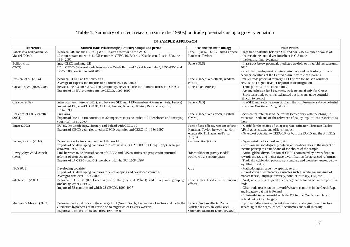
Table 1. Summary of recent research (since the 1990s) on trade potentials using a gravity equation

IN-SAMPLE APPROACH

References Studied trade relationship(s), country sample and period Econometric methodology Main results Babetskaia-Kukharchuk & Maurel (2004)

Between CIS and the EU in light of Russia's accession to the WTO 42 countries among wich 14 EU-countries, CEEC-10, Belarus, Kazakhstan, Russia, Ukraine, 1994-2001

Panel (OLS, GLS, fixed-effects, Hausman-Taylor)

Large trade potential between CIS and non-CIS countries because of: - the remaining large diversion effect in CIS trade - institutional improvements

Boillot et al. (2003)

Intra-CEEC and intra-UE UE + CEECs (bilateral trade between the Czech Rep. and Slovakia excluded), 1993-1996 and 1997-2000, prediction until 2010

Panel (OLS)

- Intra-trade below potential: predicted twofold or threefold increase until 2010 - Predicted development of intra-basin trade and particularly of trade between countries of the Central basin. Key role of Slovakia

Bussière et al. (2004) Between CEECs and the euro area Average of exports and imports of 61 countries, 1980-2002

Panel (OLS, fixed-effects, random-effects)

Smaller trade potential for large CEECs than for Balkan countries because of a higher level of regional trade integration

Caetano et al. (2002, 2003) Between the EU and CEECs and particularly, between cohesion-fund countries and CEECs Exports of 14 EU-countries and 10 CEECs, 1993-1999

Panel (fixed-effects) - Trade potential in bilateral terms. - Among cohesion fund countries, trade potential only for Greece - Short-term trade potential exhausted but long-run trade potential difficult to predict

Christie (2002) Intra-Southeast Europe (SEE), and between SEE and 3 EU-members (Germany, Italy, France) Imports of EU, non-EU OECD, CEFTA, Russia, Belarus, Ukraine, Baltic states, SEE, 1996-1999

Panel (OLS) Intra-SEE and trade between SEE and the 3 EU-members above potential except for Croatia and Yugoslavia

DeBenedictis & Vicarelli (2004)

Euro area Exports of the 11 euro-countries to 32 importers (euro countries + 21 developed and emerging countries), 1991-2000

Panel (OLS, fixed effects, 'System GMM')

Focus on the robutness of the results (which vary with the change in estimator used) and on the relevance of policy implications associated to them

Egger (2002)

EU-15, the Czech Rep., Hungary and Poland with CEEC-10 Exports of OECD countries to other OECD countries and CEEC-10, 1986-1997

Panel (fixed effects, random effects, Hausman-Taylor, between, random-effects AR(1), Hausman-Taylor AR(1))

- 'Guide' for the choice of an appropriate estimator: Hausman-Taylor AR(1) as consistent and efficient model - No export potential to CEEC-10 for both the EU-15 and the 3 CEECs

Fontagné et al. (2002)

Between developing economies and the world Exports of 53 developing countries to 75 countries (53 + 21 OECD + Hong Kong), averaged data over 1995-1996

Cross-section (OLS)

- Aggregated and sectoral analysis - Focus on methodological problems of non-linearities in the impact of income per capita on trade and of the choice of the sample

Havrylyshyn & Al-Atrash (1998)

Link between trade diversification of CEECs and CIS countries and progress in structural reforms of their economies Exports of 17 CEECs and CIS-members with the EU, 1995-1996

'Disequilibrium gravity model' Pooled cross-section (OLS)

- Actual global diversification of CEECs dominated by diversification towards the EU and higher trade diversification for advanced reformers - Trade diversification process not complete and therefore, export below equilibrium value

ITC (2003)

Developing countries Exports of 36 developing countries to 58 developing and developed countries Averaged data over 1999-2000

OLS - Methodological paper: no specific result - Introduction of explanatory variables such as a bilateral measure of market access, language diversity, conflict intensity, FDI, etc.

Jakab et al.. (2001)

Between 3 CEECs (the Czech republic, Hungary and Poland) and 5 regional groupings (including 'other CEECs') Imports of 53 countries (of which 28 OECD), 1990-1997

Panel (OLS, fixed-effects, random-effects)

- Analysis in terms of speed of convergence between actual and potential trade - Clear trade reorientation towardsWestern countries in the Czech Rep. and Hungary but not in Poland - Substantial trade potential with the EU for the Czech republic and Poland but not for Hungary

Marques & Metcalf (2003)

Between 3 regional blocs of the enlarged EU (North, South, East) across 4 sectors and under the alternative hypotheses of migration or no migration of Eastern workers Exports and imports of 25 countries, 1990-1999

Panel (Random effects, Prais-Winsten regression with Panel Corrected Standard Errors (PCSEs))

Important differences in potentials across country groups and sectors according to the degree of scale economies and skill-intensity

17

Martinez-Zarzoso et al. (2003)

Between the EU and MERCOSUR Exports of 20 countries (15 EU, 4 Mercosur, Chile), 1988-1996

Panel (OLS, fixed effects, random-effects)

- Exports of MERCOSUR to the EU below potential in 1996 but for previous years, increasing or decreasing potentials based on time specific factors. - Intra-MERCOSUR trade above potential

Paas T. (2002)

Within the Baltic Sea region (Germany, Denmark, Estonia, Finland,lLthuania, Latvia, Norway, Poland, Russia, Sweden) and between Estonia and the Baltic Sea region Exports and imports of Estonia with 46 main partners, 1997 Exports and imports of the countries of the Baltic Sea Region, 1998

Cross section

- Estonian trade with the Baltic sea region below potential I - Estonian export to CIS below potential while Estonian import from CIS above potential - Trade potential for bilateral relation between the 5 transitional countries of the region and the Scandinavian countries

Péridy (2004)

Between the U.S. and Australia, the ASEAN, the Southern African Customs Union (SACU), Middle-East and North-African (MENA) countries US exports to 56 OECD and emerging countries, 1982-2001

Panel (GMM) Also out-of-sample estimations

- Limited trade (and FDI) potential for the US with their new parnters - Smaller potentials with the dynamic model.

Van Bergeijk & Oldersma (1990)

Trade potential from the normalisation of East-West relations, especially from the German unification Exports of 49 developed and developing countries, 1985

Cross-section (OLS) - Potential trade from the détente for CEECs and EFTA but not for other regions - Negative effect of the German unification

OUT-OF-SAMPLE APPROACH

References Studied trade relationship(s) Comparison group of countries Econometric methodology Main results Abraham & Van Hove (2005) Trade potentials from China's entry in 3 RTAs

(Asean, Apec and 'Asian Apec') Exports of 23 countries from Asean and Apec, 1992-2000

Panel (OLS, fixed effects, random effects)

Large trade potential, particularly in case of China's integration into ASEAN

Adam & Boillot (1995)

Between France and 6 CEECs (Bulgaria, the Czech Rep., Hungary, Poland, Romania, Slovakia, Russia), 1994

Exports of France to its 100 first clients (except CEEC and CIS), 1992

Cross-section (OLS)

- French exports to CEEcs below potential. - Test of different hypotheses of catching up of CEECs on France

Arnon, Spivak & Weinblatt (1996)

Between Jordan, the Palestinian entity and Israel with alternative hypotheses of free-trade agreements, 1992

Exports and imports of 16 countries (Israel, Jordan, Syria, Ethiopia, Sudan, China, India, Indonesia, Turkey, Korea, Iran, Saudi Arabia, Yemen, the USA, Japan, Germnay), 1991

Cross-section (OLS) Under normal economic and political conditions, trade expected to develop beetween Israel and the Palestinian entity but to be modest between Israel and Jordan-

Baldwin (1993)

Between EFTA and 12 CEECs (Albania, Baltic States, Bulgaria, Croatia, the Czech Rep., Hungary, Poland, Romania, Slovakia, Slovenia)

Same sample as in Wang & Winters (1992)

Updating and extending of Wang & Winters (1992) to 1989

- Large export trade potential for EFTA to CEECs due to the elimination of trade barriers and to CEECs' catching-up to Western levels of per capita income - Allows Baldwin to suggest an Eastern enlargement of EFTA

Baldwin (1994)

Within CEECs and between them and Western countries, 1989

Imports among EC and EFTA, and between these countries and Canada, Japan, Turkey, the USA, 1979-1988

Panel (OLS, random effects)

- Large medium-run and long-run export trade potential for West European countries to CEECs - No intra-CEEC trade potential in the medium-run but in the long-run

Batra (2004) India Exports and imports of 146 countries (ASEAN, GCC, SAARC), 2000

Cross-section (OLS) Potential maximum for Asia-Pacific (especially with China), followed by Western Europe (expecially France, Italy and the UK) and North America

Brulhart & Kelly (1999)

Between Ireland and 5 CEECs (the Czech Rep., Estonia, Hungary, Poland, Slovenia), 1994 and long-run projection to 2020

Imports of 13 OECD and 11 emerging countries, 1994

Cross-section (OLS) - Irish exports to CEEC close to their potential - Irish imports from CEEC only half of their potential

Buch & Piazolo (2001) Between OECD and CEEC-10, 1998 Exports and imports of 9 OECD countries with 69 non-transition countries, 1998

Cross-section (OLS) - OECD exports to CEEC-10 below potential except for Hungary. - OECD imports from CEEC-10 below potential except for Austria and Germany

Dimelis & Gatsios (1995) Between Greece and 6 CEECs (Albania, Bulgaria, Czechoslovakia, Hungary, Poland, Romania), 1989

Exports of 17 EC and EFTA countries to 20 importing countries, 1981-1992 and 1988-1992

Projection of estimates of Baldwin (1994)

- Large export trade potential for Greece to the 6 CEECs, except for Albania and especially with the Visegrad countries - Smaller export trade potential for the 6 CEECs to Greece

18

Ekholm et al. (1996)

Within 13 countries from the Middle East and North Africa, and between them and European countries under normal political relations, 1989 and medium-run and long-run projections

Imports of 13 OECD countries and 11 outward-oriented developing countries, 1990

Cross-section (OLS)

-No large overall potential within the region and with European countries - Long-run potential higher than short-or medium-run potential

Festoc (1997)

Between 5 CEECs (the Czech Republic, Hungary, Poland, Romania, Slovakia) and 5 EU-members, 1990

Exports of the EU (except Portugal), EFTA, the USA, Canada, Japan, Australia, New-Zealand, 1980-1992

Panel (OLS, random-effects) - Diminution of the EU-CEECs trade potential since 1990 - Import trade potential of CEECs from the EU lower than export trade potential

Fidrmuc (1999) Between Slovakia and 6 EU-countries; between Slovakia and 3 CEECs (the Czech Rep., Hungary, Poland) under 3 scenarios (no Eastward enlargement, enlargement with or without Slovakia), 1996

23 OECD-countries, 1989 Cross-section (OLS)

Trade with the EU, Hungary and Poland below potential but trade with the Czech Republic 9 times above potential

Fontagné et al. (1999)

Between 4 CEECs (former Czechoslovakia, Hungary, Poland, Romania) and the EU, 1990-1995

Exports and imports of 21 OECD-countries, 1980-1995

Panel (fixed-effects, random-effects)

- Exhausted short-term trade potential but non-exhausted long-run trade potential, except between Hungary and Germany or Austria - Change in sectoral patterns: potential of gain in product variety - Methodologically, problem of the choice of the fixed-effects

Gros & Gonciarz (1996)

Within 3 CEECs (Czechoslovakia, Hungary and Poland) and between them and the EU, 1992

Same sample as in Baldwin (1994)

Panel (OLS, random effects) Updating of Baldwin (1994) to 1992

Contrary to Baldwin's (1994) results, CEECs' trade reorientation already achieved in 1992 and therefore, no remaining unexhausted potential with the EU and no need of special protection

Hamilton & Winters (1992)

Between Bulgaria, CSFR, GDR, Hungary, Poland, Romania, USSR and 5 regional goupings (CEECs included), 1985

Imports of 19 industrial countries and 57 LDCs Averaged data over 1984-1986

Cross-section (OLS)

- Intra- trade above potential for the USSR, Czecoslovakia, Bulgaria and DDR but not for Hungary and Romania and above all for Poland - East-West trade below potential - Trade with LDCs least below potential

Havrylyshyn & Pritchett (1991)

Between 6 CEECs (Bulgaria, Czechoslovakia, Hungary, Poland, Romania, Yugoslovia) and several regional groupings (CEECs included), 1980-82 and 1986-87

Exports and imports of 2 samples of countries with 95 non-socialist partners: - 14 large semi-industrialised countries - 21 non-oil exporting countries Averaged data over 1980-1982

Cross-section (Tobit maximum likehood)

- Intra-CEEC trade above potential - Trade between the 6 CEECs and Northern Europe below potential

McPherson & Trumbull (2003)

Between the US and Cuba, 1996-2000 Imports of 101 developed and developing countries, 1996-2000

Panel (OLS, fixed-effects, random-effects, Hausman-Taylor)

Methodological paper: the comparison of several estimators reveals the superiority of the Hausman-Taylor method

Nilsson (2000)

Within the candidate countries and between them and the EU

Imports between the EU and EFTA, within NAFTA, between Australia and New-Zealand, between the EU and Turkey, averaged data over 1995-1996

Cross-section (OLS)

- Still some unused potential trade between the EU and the candidate countries but decreasing - Intra-CEECs' trade above potential

Péridy (2005a) Between the US and Middle-East and North-African (MENA) countries, 1976-2001

Exports of 20 OECD countries to 43 main partners, 1975-2001

Panel (Fixed-effects, random-effects, Hausman-Taylor)

- Increasing US export potential, particularly to Maghreb countries - Results of the in-of-sample approach similar to those of the out-of-sample approach because of the very low share of MENA in total US exports

Péridy (2005b) Between the EU and its new Eastern and Southern neighbors,

Exports of 65 EU partners, 1993-2003 Panel (Fixed-effects, random-effects, Hausman-Taylor)

- Substantial NNCs' export potential to the EU, although limited for Mediterranean countries - No impact ot the implementation of the 'Wider Europe Initiative' - Extension of the analysis to Middle-East and Gulf countries which also reveals a substantial export potential to the EU

Wang & Winters (1992)

Between CEECs (Bulgaria, Czescholovakia, Eastern Germany, Hungary, Poland, Romania, USSR) and 5 regional groupings (CEECs, included), 1985

Imports and exports of 76 non-CEECs (Yugoslavia included) Averaged data over 1984-86

Cross-section (OLS) - Intra-trade close to or above potential except for Poland - Trade of CEECs with market economies below one quarter of its potential - Germany followed by the USA as main gainer

19

Table 2. Share of intra-regional trade, 1994-2003, percentage

1994 1995 1996 1997 1998 1999 2000 2001 2002 2003 EU 0,61 0,64 0,63 0,61 0,61 0,59 0,58 0,56 0,58 0,58 CEEC8 0,12 0,12 0,11 0,11 0,10 0,10 0,10 0,10 0,10 0,11 Balkans n.a. n.a 0,05 0,05 0,07 0,11 0,09 0,08 0,08 0,04

Source: Authors' calculation based on COMTRADE.

Table 3. Share of the EU in CEECs' trade, 1994-2002, percentage

1994 1995 1996 1997 1998 1999 2000 2001 2002 Share of CEECs' imports from the EU CEEC8 0,62 0,63 0,63 0,64 0,67 0,67 0,64 0,64 0,63 Balkans 0,50 0,51 0,52 0,53 0,56 0,58 0,55 0,57 0,57 Share of CEECs' exports to the EU CEEC8 0,61 0,62 0,61 0,61 0,65 0,68 0,67 0,66 0,65 Balkans 0,48 0,48 0,48 0,51 0,55 0,57 0,57 0,60 0,60

Source: Boudier-Bensebaa & Lamotte (2005).

Table 4. Commodity composition of intra-CEECs' trade (5 first products), 1993 and 2002, percentage of exports

1993 2002 Exporter: CEEC8 - Importer:CEEC8

Iron and steel 7,27 Refined petroleum products 8,74 Refined petroleum products 5,29 Iron and steel 5,60

Miscellaneous hardware 4,80 Plastic articles 5,12 Coke 4,40 Paper 4,89

Plastic articles 4,13 Cars and cycles 4,42 Exporter: CEEC8 - Importer: Balkans

Paper 7,03 Paper 6,64 Iron and steel 5,86 Plastic articles 5,30

Leathers 5,17 Iron and steel 4,97 Pharmaceuticals 4,44 Toiletries 4,67 Plastic articles 3,93 Miscellaneous hardware 4,59

Exporter: Balkans - Importer: Balkans Refined petroleum products 9,69 Refined petroleum products 14,66

Non ferrous metals 5,46 Non elsewhere class. products 6,53 Other edible agricultural products 5,32 Manufactured tobaccos 5,40

Iron and steel 4,73 Beverage 3,99 Cereals 4,52 Iron and steel 3,75

Exporter: Balkans - Importer: CEEC8 Refined petroleum products 11,43 Refined petroleum products 9,04

Preserved fruits 4,67 Clothing 5,26 Pharmaceuticals 4,38 Non edible agricultural products 4,89

Electric apparatus 4,14 Plastic articles 4,08 Other edible agricultural products 3,76 Miscellaneous hardware 4,02

Source: Boudier-Bensebaa & Lamotte (2005).

20

Table 5. Definitions and expected impacts of explanatory variables

Name Label Definition Source Expected impact

Growth domestic product

GDPi or j GDP of i or j in current US dollars

WDI, World Bank

Positive

Weighted distance W.Dist. ij Distance in kilometers between the major cities of i and j weighted by the share of their population

CEPII Negative

Distance Distanceij Geodesic distance between capitals of i and j in kilometers

Haveman's website

Negative

Border Borderij 1 if the i and j share a common border, 0 otherwise

CEPII Positive

Common language Comlangij 1 if i and j share a common language, 0 otherwise

CEPII Positive

Infrastructure Infrai or j Density of paved roads in i or j per square kilometer

WDI, World Bank

Positive

Population Popi or j Population of i or j WDI, World Bank

Undetermined

Area Areai or j Area of i or j in square kilometer

WDI, World Bank

Undetermined

Table 6. Estimations results

(1) (2) (3) (4) Dep. var.: Ln(Mijt) OLS FEM REM HTM

Ln(GDPi)

0,808 a

(0,01) 0,801 a

(0,04) 0,779 a

(0,03) 0,792 a

(0,04) Ln(GDPj)

0,808 a

(0,01) 0,665 a

(0,04) 0,729 a

(0,03) 0,673 a

(0,04) Ln(W.Dist.ij) -1.146a

(-0.04) - -0,997 a

(0,09) -0,565 a

(0,18) Borderij

0,084b

(0,04) - 0,272 c

(0,14) 0,626 a

(0,20) Languageij

0,305 a

(0,05) - 0,207

(0,19) 0,395 c

(0,19) Ln(Infrai)

-0,157 a

(0,02) 0,023 (0,02)

0,013 (0,02)

0,021

(0,02) Ln(Infraj)

-0,106 a

(0,02) 0,040 c

(0,02) 0,030 c

(0,02) 0,042 b

(0,02) Constant 13,228 a

(-21,33) -17,394 a

(-15,42) -11,489a

(-9,18) -13,504 a

(-7,36) # obs. 1676 1676 1676 1676

R2 0,88 0,74 0,88 - Notes: a, b and c denote significance at the 1%, 5% and 10% levels. OLS, FEM, REM and HTM indicates respectively Ordinary Least Square, Fixed-Effect, Random Effect and Hausman-Taylor models. Standard errors are in parentheses. The adjusted R2 for OLS and the overall R2

for FEM and REM are displayed. HTM: endogeneous variables=Ln(GDPi), Ln(GDPj), Ln(W.Dist.ij).

21

Table 7. Robustness checks

(5) (6) (7) (8) Dep. var.: Ln(Mijt) HTM HTM HTM HTM

Ln(GDPi)

0,792 a

(0,04) 0,614 a

(0,04) 0,775 a

(0,03) 0,792 a

(0,04) Ln(GDPj)

0,673 a

(0,04) 0,443 a

(0,04) 0,691 a

(0,03) 0,673 a

(0,04) Ln(Distanceij)

-0,524 a

(0,16) Ln(W. Distij) -0,565 a

(0,18) 0,513 (1,16)

-0,919a

(0.31)

Borderij

0,626 a

(0,20) -2,218 (1,36)

0,235 (0,33)

0,572 a

(0,22) Languageij

0,395 c

(0,19) 4,034 c

(1,54) 0,406 c

(0,21) 0,392 c

(0,23) Ln(Infrai)

0,021

(0,02) 0,056 (0,01)

0,041

(0,02) 0,042 (0,02)

Ln(Infraj)

0,042 b

(0,02) 0,039 a

(0,01) 0,022a

(0,02) 0,021a

(0,02)

Ln(Popi)

2.260 a

(0,25)

Ln(Popj)

2,685 a

(0,25)

Ln(Areai)

0,122 (0,09)

Ln(Areaj)

0,128 (0.09)

Constant -13,504 a

(-7,36) -92,300 a

(9,04) -13,432 a

(1,64) -13,146 a

(11,77) # obs. 1676 1676 1676 1676

Notes: a, b and c denote significance at the 1%, 5% and 10% levels. HTM indicates Hausman-Taylor model. Standard errors are in parentheses. HTM: endogeneous variables=Ln(GDPi), Ln(GDPj), Ln(W.Dist.ij).

Table 8. Highest actual/potential trade ratios, 1994-1995

Importer Exporter Actual trade Potential trade Actual/Potential tradeMKD SVN 139250000 6145658,399 22,658 CZE SVK 2559500000 145237308,7 17,623 SVK CZE 2187000000 128453914,1 17,026 MKD BGR 248700000 20828001,73 11,941 SVN MKD 83022428 7165676,112 11,586 LTU EST 53070967 4663476,668 11,380 EST LTU 41103388 4455133,423 9,226

MKD HRV 57841336 6581700,414 8,788 MKD SCG 131250000 15627157,38 8,399

22

LVA EST 67759592 9607357,818 7,053 HRV SVN 672750000 110299309,2 6,099 LVA LTU 87297584 14793628,56 5,901 LTU LVA 92269614 15723441,37 5,868 EST LVA 50496052 9755011,104 5,176 SVN HRV 536900000 109585830,3 4,899 HRV MKD 31849643 7724053,226 4,123 SVN CZE 212250000 52291445,73 4,059 HUN CZE 352500000 108787729,3 3,240 LTU CZE 49174268 17205326,37 2,858 HRV CZE 119444804 48267197 2,475

Source: Authors' calculation based on COMTRADE. Trade flows are expressed in millions of US dollars.

Table 9. Highest actual/potential trade ratios, 1998-1999

Importer Exporter Actual trade Potential trade Actual/Potential tradeMKD SVN 152600000 6575261,592 23,208 LTU EST 142550000 8371805,021 17,027 MKD SCG 214650000 13313759,35 16,122 LVA EST 200050000 16142297,67 12,393 SCG MKD 182750000 15247576,12 11,986 SVK CZE 2129500000 180393452,6 11,805 EST LTU 72830213 7541633,172 9,657

MKD HRV 1928500000 200230013 9,631 CZE SVK 63384562 7186288,836 8,820 SCG BIH 224300000 27354192,59 8,200 LTU LVA 208500000 25693029,28 8,115 LVA LTU 54009870 8711170,071 6,200 HRV MKD 217500000 36048432,55 6,034 SVN MKD 92903855 15481756,75 6,001 EST LVA 41703328 7797561,729 5,348 HRV BIH 668950000 149196466 4,484 HRV SVN 88908056 21188801,84 4,196 SVN BIH 51112724 13167143,02 3,882 ALB BGR 25841985 6675886,861 3,871 SVN CZE 272350000 71936338,38 3,786

Source: Authors' calculation based on COMTRADE. Trade flows are expressed in millions of US dollars.

Table 10. Highest actual/potential trade ratios 2002-2003

Importer Exporter Actual trade Potential trade Actual/Potential tradeMKD SVN 134250000 8494748,596 15,804 EST LTU 196450000 13123737,73 14,969 LVA EST 293100000 28057486,36 10,446 BIH SVN 173750000 16782854,42 10,353 SVK CZE 2876000000 279139993,4 10,303 LVA LTU 453550000 45118390,23 10,052 MKD SCG 198850000 20265822,25 9,812

23

CZE SVK 2397000000 310715767,3 7,714 MKD HRV 59343706 9402854,225 6,311 EST LVA 163350000 26872679,9 6,079 BIH HRV 321250000 56449984,32 5,691

MKD BGR 138650000 29745198,7 4,661 LTU EST 67650000 14594832,88 4,635 HUN CZE 1006750000 246419263,4 4,086 SVN BIH 76916070,5 19310263,84 3,983 ROM CZE 418950000 107059023,4 3,913 CZE HUN 922850000 251935151,5 3,663 SCG SVN 121150000 34230527,52 3,539 ROM SVK 202150000 61834663,24 3,269 EST POL 170950000 52638455,24 3,248

Source: Authors' calculation based on COMTRADE. Trade flows are expressed in millions of US dollars.

Appendix Appendix 1. Geographical breakdown

CEECs8: Czech Republic, Estonia, Hungary, Latvia, Lituania, Poland, Slovakia, Slovenia. Balkans: Albania, Bosnia and Herzegovina, Bulgaria, Croatia, Macedonia, Romania, Serbia and Montenegro.

Appendix 2. Actual/potential trade ratios of CEECs, 1994-95, 1998-99, 2002-03 .Importer Exporter 94-95 98-99 02-03 Importer Exporter 94-95 98-99 02-03

ALB BGR - 3,871 0,143 BIH LVA - 0,000 1,219 ALB BIH - 0,026 0,510 BIH MKD - 0,000 1,099 ALB CZE - 0,369 0,000 BIH POL - 0,000 0,547 ALB EST - 0,000 2,569 BIH ROM - 0,000 0,574 ALB HRV - 1,244 0,555 BIH SCG - 0,000 0,635 ALB HUN - 0,960 0,006 BIH SVK - 0,000 10,353 ALB LTU - 0,004 0,079 BIH SVN - 0,000 0,033 ALB LVA - 0,000 0,755 CZE ALB 0,010 0,043 3,241 ALB MKD - 1,773 0,103 CZE BGR 0,620 0,680 0,926 ALB POL - 0,047 0,840 CZE BIH 0,033 0,080 0,176 ALB ROM - 0,509 0,524 CZE EST 0,423 1,115 0,764 ALB SCG - 0,084 0,062 CZE HRV 0,641 0,499 0,422 ALB SVK - 0,000 2,087 CZE HUN 1,689 2,941 3,663 ALB SVN - 2,286 0,013 CZE LTU 0,431 0,344 0,513 BGR ALB - 0,007 0,056 CZE LVA 0,296 0,243 0,326 BGR BIH - 0,011 3,241 CZE MKD 0,863 0,386 0,192 BGR CZE - 3,333 0,102 CZE POL 1,466 1,750 2,280 BGR EST - 0,055 0,817 CZE ROM 0,238 0,359 0,968 BGR HRV - 0,220 1,960 CZE SCG 0,013 0,371 0,410 BGR HUN - 1,239 0,675 CZE SVK 17,623 9,631 7,714 BGR LTU - 0,370 0,139 CZE SVN 1,697 2,070 2,299 BGR LVA - 0,100 0,597 EST ALB - 0,000 0,007 BGR MKD - 1,281 1,516 EST BGR 0,831 1,364 0,771 BGR POL - 1,017 1,557 EST BIH - 0,012 0,034 BGR ROM - 0,738 0,469 EST CZE 1,659 1,864 2,896 BGR SCG - 0,735 2,151 EST HRV 0,149 0,130 0,169 BGR SVK - 1,632 2,268 EST HUN 1,578 2,015 2,659

24

BGR SVN - 1,207 0,018 EST LTU 9,226 9,657 14,969 BIH ALB - 0,000 0,265 EST LVA 5,176 6,001 6,079 BIH BGR - 0,000 1,677 EST MKD 0,039 0,089 0,087 BIH CZE - 0,000 0,016 EST POL 0,698 2,081 3,248 BIH EST - 0,000 5,691 EST ROM 0,034 0,085 0,367 BIH HRV - 0,000 1,827 EST SCG 0,002 0,107 0,138 BIH HUN - 0,000 0,075 EST SVK 0,750 0,991 1,592 BIH LTU - 0,000 0,013 EST SVN 0,247 0,684 1,063 HRV ALB 0,502 0,077 0,033 LTU LVA 5,868 8,200 1,617 HRV BGR 1,073 0,465 1,020 LTU MKD 0,008 0,009 0,013 HRV BIH 0,510 3,057 2,986 LTU POL 1,291 2,046 0,936 HRV CZE 2,475 2,397 3,072 LTU ROM 0,157 0,060 0,127 HRV EST 0,022 0,084 0,168 LTU SCG 0,019 0,090 0,050 HRV HUN 1,092 1,287 1,548 LTU SVK 2,022 1,385 0,901 HRV LTU 0,155 0,007 0,154 LTU SVN 1,049 1,443 0,969 HRV LVA 0,197 0,096 0,095 LVA ALB - 0,000 0,002 HRV MKD 4,123 6,200 2,914 LVA BGR 1,181 2,247 1,105 HRV POL 0,623 0,677 1,344 LVA BIH - 0,000 0,001 HRV ROM 0,419 0,369 1,657 LVA CZE 1,012 2,117 2,068 HRV SCG - 0,296 0,878 LVA EST 7,053 12,393 10,446 HRV SVK 1,893 1,179 1,030 LVA HRV 0,082 0,120 0,227 HRV SVN 6,099 4,484 2,598 LVA HUN 0,744 1,672 1,409 HUN ALB 0,057 0,010 0,010 LVA LTU 5,901 8,115 10,052 HUN BGR 0,676 0,870 0,846 LVA MKD - 0,015 0,002 HUN BIH 0,018 0,114 0,355 LVA POL 0,856 2,302 2,933 HUN CZE 3,240 3,655 4,086 LVA ROM 0,025 0,093 0,085 HUN EST 0,212 0,532 1,842 LVA SCG 0,033 0,239 0,133 HUN HRV 0,428 0,284 0,297 LVA SVK 0,756 1,278 2,158 HUN LTU 1,301 0,165 0,664 LVA SVN 0,380 0,671 1,060 HUN LVA 0,289 0,101 0,180 MKD ALB 1,124 0,300 0,178 HUN MKD 0,590 0,253 0,094 MKD BGR 11,941 4,196 4,661 HUN POL 1,230 2,076 2,884 MKD BIH 0,417 2,171 2,431 HUN ROM 0,983 1,354 1,938 MKD CZE 2,393 1,306 0,692 HUN SCG 0,008 0,387 0,340 MKD EST 0,327 0,040 0,074 HUN SVK 1,858 1,848 1,921 MKD HRV 8,788 8,820 6,311 HUN SVN 0,750 1,099 1,073 MKD HUN 1,076 1,949 1,500 LTU ALB - 0,000 0,002 MKD LTU 0,047 0,005 0,025 LTU BGR 2,082 1,508 0,729 MKD LVA 0,037 0,021 0,001 LTU BIH - 0,012 0,012 MKD POL 0,549 1,102 0,927 LTU CZE 2,858 3,100 1,527 MKD ROM 1,381 0,733 0,671 LTU EST 11,380 17,027 4,635 MKD SCG 8,399 16,122 9,812 LTU HRV 0,049 0,228 0,154 MKD SVK 0,613 0,814 0,607 LTU HUN 1,874 2,317 0,945 MKD SVN 22,658 23,208 15,804 POL ALB - 0,018 0,001 SCG LTU - 0,060 0,108 POL BGR 0,422 0,521 0,636 SCG LVA - 0,017 0,011 POL BIH 0,004 0,049 0,069 SCG MKD - 11,986 2,823 POL CZE 1,664 2,254 2,182 SCG POL - 0,710 0,332 POL EST 0,375 0,319 0,558 SCG ROM - 1,621 0,686 POL HRV 0,527 0,376 0,199 SCG SVK - 1,826 1,092 POL HUN 1,369 2,097 2,333 SCG SVN - 2,210 3,539 POL LTU 0,488 0,682 0,640 SVK ALB 0,101 0,128 0,007

25

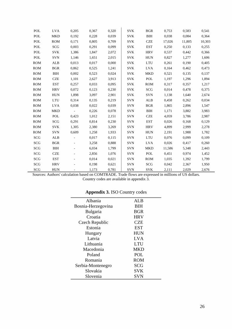
POL LVA 0,205 0,367 0,320 SVK BGR 0,753 0,583 0,541 POL MKD 0,192 0,228 0,039 SVK BIH 0,038 0,084 0,364 POL ROM 0,171 0,805 0,709 SVK CZE 17,026 11,805 10,303 POL SCG 0,003 0,291 0,099 SVK EST 0,250 0,133 0,255 POL SVK 1,386 1,847 2,072 SVK HRV 0,537 0,442 0,366 POL SVN 1,146 1,651 2,015 SVK HUN 0,827 1,277 1,606 ROM ALB 0,013 0,017 0,000 SVK LTU 0,261 0,190 0,405 ROM BGR 0,862 0,525 1,241 SVK LVA 0,164 0,462 0,473 ROM BIH 0,002 0,523 0,024 SVK MKD 0,521 0,135 0,137 ROM CZE 1,101 2,627 3,913 SVK POL 1,197 1,296 1,894 ROM EST 0,257 0,033 0,095 SVK ROM 0,317 0,357 1,217 ROM HRV 0,072 0,123 0,230 SVK SCG 0,014 0,478 0,375 ROM HUN 1,898 3,097 2,901 SVK SVN 1,138 1,640 2,674 ROM LTU 0,314 0,135 0,219 SVN ALB 0,458 0,262 0,034 ROM LVA 0,038 0,022 0,039 SVN BGR 1,865 2,896 1,547 ROM MKD - 0,226 0,078 SVN BIH 1,171 3,882 3,983 ROM POL 0,423 1,012 2,151 SVN CZE 4,059 3,786 2,987 ROM SCG 0,291 0,814 0,230 SVN EST 0,026 0,168 0,129 ROM SVK 1,305 2,380 3,269 SVN HRV 4,899 2,999 2,278 ROM SVN 0,609 1,258 1,933 SVN HUN 2,191 1,988 1,782 SCG ALB - 0,017 0,115 SVN LTU 0,076 0,099 0,109 SCG BGR - 3,258 0,888 SVN LVA 0,026 0,417 0,260 SCG BIH - 6,034 1,799 SVN MKD 11,586 5,348 2,443 SCG CZE - 2,856 1,076 SVN POL 0,451 0,974 1,452 SCG EST - 0,014 0,021 SVN ROM 1,035 1,392 1,799 SCG HRV - 0,198 0,621 SVN SCG 0,042 2,367 1,950 SCG HUN - 1,173 0,781 SVN SVK 2,111 2,029 2,676

Sources: Authors' calculation based on COMTRADE. Trade flows are expressed in millions of US dollars. Country codes are available in appendix 3.

Appendix 3. ISO Country codes

Albania ALB Bosnia-Herzegovina BIH

Bulgaria BGR Croatia HRV

Czech Republic CZE Estonia EST Hungary HUN Latvia LVA

Lithuania LTU Macedonia MKD

Poland POL Romania ROM

Serbia-Montenegro SCG Slovakia SVK Slovenia SVN

26