Description of affy

Laurent Gautier, Rafael Irizarry, Leslie Cope, and Ben Bolstad

April 30, 2018

Contents

1 Introduction 2

2 Changes for affy in BioC 1.8 release 3

3 Getting Started: From probe level data to expression values 33.1 Quick start . . . . . . . . . . . . . . . . . . . . . . . . . . . . . . . . . . 43.2 Reading CEL file information . . . . . . . . . . . . . . . . . . . . . . . . 53.3 Expression measures . . . . . . . . . . . . . . . . . . . . . . . . . . . . . 7

3.3.1 expresso . . . . . . . . . . . . . . . . . . . . . . . . . . . . . . . . 73.3.2 MAS 5.0 . . . . . . . . . . . . . . . . . . . . . . . . . . . . . . . . 93.3.3 Li and Wong’s MBEI (dchip) . . . . . . . . . . . . . . . . . . . . 93.3.4 C implementation of RMA . . . . . . . . . . . . . . . . . . . . . . 10

4 Quality Control through Data Exploration 114.1 Accessing PM and MM Data . . . . . . . . . . . . . . . . . . . . . . . . 124.2 Histograms, Images, and Boxplots . . . . . . . . . . . . . . . . . . . . . . 144.3 RNA degradation plots . . . . . . . . . . . . . . . . . . . . . . . . . . . . 18

5 Normalization 20

6 Classes 206.1 AffyBatch . . . . . . . . . . . . . . . . . . . . . . . . . . . . . . . . . . . 206.2 ProbeSet . . . . . . . . . . . . . . . . . . . . . . . . . . . . . . . . . . . . 21

7 Location to ProbeSet Mapping 22

8 Configuring the package options 27

9 Where can I get more information? 27

1

A Previous Release Notes 28A.1 Changes in versions 1.6.x . . . . . . . . . . . . . . . . . . . . . . . . . . . 28A.2 Changes in versions 1.5.x . . . . . . . . . . . . . . . . . . . . . . . . . . . 28A.3 Changes in versions 1.4.x . . . . . . . . . . . . . . . . . . . . . . . . . . . 28

1 Introduction

The affy package is part of the BioConductor1 project. It is meant to be an extensible,interactive environment for data analysis and exploration of Affymetrix oligonucleotidearray probe level data.

The software utilities provided with the Affymetrix software suite summarizes theprobe set intensities to form one expression measure for each gene. The expressionmeasure is the data available for analysis. However, as pointed out by Li and Wong(2001), much can be learned from studying the individual probe intensities, or as we callthem, the probe level data. This is why we developed this package. The package includesplotting functions for the probe level data useful for quality control, RNA degradationassessments, different probe level normalization and background correction procedures,and flexible functions that permit the user to convert probe level data to expressionmeasures. The package includes utilities for computing expression measures similar toMAS 4.0’s AvDiff (Affymetrix, 1999), MAS 5.0’s signal (Affymetrix, 2001), DChip’sMBEI (Li and Wong, 2001), and RMA (Irizarry et al., 2003b).

We assume that the reader is already familiar with oligonucleotide arrays and with thedesign of the Affymetrix GeneChip arrays. If you are not, we recommend the Appendixof the Affymetrix MAS manual Affymetrix (1999, 2001).

The following terms are used throughout this document:

probe oligonucleotides of 25 base pair length used to probe RNA targets.

perfect match probes intended to match perfectly the target sequence.

PM intensity value read from the perfect matches.

mismatch the probes having one base mismatch with the target sequence intended toaccount for non-specific binding.

MM intensity value read from the mis-matches.

probe pair a unit composed of a perfect match and its mismatch.

affyID an identification for a probe set (which can be a gene or a fraction of a gene)represented on the array.

probe pair set PMs and MMs related to a common affyID.

1http://bioconductor.org/

2

CEL files contain measured intensities and locations for an array that has been hy-bridized.

CDF file contain the information relating probe pair sets to locations on the array.

Section 2 describes the main differences between version 1.5 and this version (1.6).Section 3 describes a quick way of getting started and getting expression measures. Sec-tion 4 describes some quality control tools. Section 5 describes normalization routines.Section 6 describes the different classes in the package. 7 describes our strategy tomap probe locations to probe set membership. Section 8 describes how to change thepackage’s default options. Section ?? describes earlier changes.

Note: If you use this package please cite Gautier et al. (2003) and/or Irizarry et al.(2003a).

2 Changes for affy in BioC 1.8 release

There were relatively few changes.

� MAplot now accepts the argument plot.method which can be used to call smooth-Scatter.

� normalize.quantiles.robust has had minor changes.

� ReadAffy can optionally return the SD values stored in the cel file.

� The C parsing code has been moved to the affyio package, which is now a depen-dency of the affy package. This change should be transparent to users as affyiowill be automatically loaded when affy is loaded.

� Added a cdfname argument to justRMA and ReadAffy to allow for the use ofalternative cdf packages.

3 Getting Started: From probe level data to expres-

sion values

The first thing you need to do is load the package.

R> library(affy) ##load the affy package

This release of the affy package will automatically download the appropriate cdf environ-ment when you require it. However, if you wish you may download and install the cdfenvironment you need from http://bioconductor.org/help/bioc-views/release/

data/annotation/ manually. If there is no cdf environment currently built for yourparticular chip and you have access to the CDF file then you may use the makecdfenvpackage to create one yourself. To make the cdf packaes, Microsoft Windows users willneed to use the tools described in http://www.murdoch-sutherland.com/Rtools/.

3

3.1 Quick start

If all you want is to go from probe level data (Cel files) to expression measures here aresome quick ways.

If you want is RMA, the quickest way of reading in data and getting expressionmeasures is the following:

1. Create a directory, move all the relevant CEL files to that directory

2. If using linux/unix, start R in that directory.

3. If using the Rgui for Microsoft Windows make sure your working directory containsthe Cel files (use “File -> Change Dir” menu item).

4. Load the library.

R> library(affy) ##load the affy package

5. Read in the data and create an expression, using RMA for example.

R> Data <- ReadAffy() ##read data in working directory

R> eset <- rma(Data)

Depending on the size of your dataset and on the memory available to your system,you might experience errors like ‘Cannot allocate vector . . . ’. An obvious option is toincrease the memory available to your R process (by adding memory and/or closingexternal applications2. An another option is to use the function justRMA.

R> eset <- justRMA()

This reads the data and performs the ‘RMA’ way to preprocess them at the C level.One does not need to call ReadAffy, probe level data is never stored in an AffyBatch.rma continues to be the recommended function for computing RMA.

The rma function was written in C for speed and efficiency. It uses the expressionmeasure described in Irizarry et al. (2003b).

For other popular methods use expresso instead of rma (see Section 3.3.1). Forexample for our version of MAS 5.0 signal uses expresso (see code). To get mas 5.0 youcan use

R> eset <- mas5(Data)

which will also normalize the expression values. The normalization can be turned offthrough the normalize argument.

2UNIX-like systems users might also want to check ulimit and/or compile R and the package for 64bits when possible.

4

In all the above examples, the variable eset is an object of class ExpressionSet

described in the Biobase vignette. Many of the packages in BioConductor work onobjects of this class. See the genefilter and geneplotter packages for some examples.

If you want to use some other analysis package, you can write out the expressionvalues to file using the following command:

R> write.exprs(eset, file="mydata.txt")

3.2 Reading CEL file information

The function ReadAffy is quite flexible. It lets you specify the filenames, phenotype, andMIAME information. You can enter them by reading files (see the help file) or widgets(you need to have the tkWidgets package installed and working).

R> Data <- ReadAffy(widget=TRUE) ##read data in working directory

This function call will pop-up a file browser widget, see Figure 1, that provides an easyway of choosing cel files.

5

Figure 1: Graphical display for selecting CEL files. This widget is part of the tkWidgetspackage. (function written by Jianhua (John) Zhang).

Next, a widget (not shown) permits the user to enter the phenoData. Finally the awidget is presented for the user to enter MIAME information.

Notice that it is not necessary to use widgets to enter this information. Pleaseread the help file for more information on how to read it from flat files or to enter itprogrammatically.

The function ReadAffy is a wrapper for the functions read.affybatch, tkSample-Names, read.AnnotatedDataFrame, and read.MIAME. The function read.affybatch hassome nice feature that make it quite flexible. For example, the compression argumentpermit the user to read compressed CEL files. The argument compress set to TRUEwill inform the readers that your files are compressed and let you read them while theyremain compressed. The compression formats zip and gzip are known to be recognized.

A comprehensive description of all these options is found in the help file:

R> ?read.affybatch

R> ?read.AnnotatedDataFrame

R> ?read.MIAME

6

3.3 Expression measures

The most common operation is certainly to convert probe level data to expression values.Typically this is achieved through the following sequence:

1. reading in probe level data.

2. background correction.

3. normalization.

4. probe specific background correction, e.g. subtracting MM .

5. summarizing the probe set values into one expression measure and, in some cases,a standard error for this summary.

We detail what we believe is a good way to proceed below. As mentioned the functionexpresso provides many options. For example,

R> eset <- expresso(Dilution, normalize.method="qspline",

bgcorrect.method="rma",pmcorrect.method="pmonly",

summary.method="liwong")

This will store expression values, in the object eset, as an object of class Expres-

sionSet (see the Biobase package). You can either use R and the BioConductor packagesto analyze your expression data or if you rather use another package you can write itout to a tab delimited file like this

R> write.exprs(eset, file="mydata.txt")

In the mydata.txt file, row will represent genes and columns will represent sam-ples/arrays. The first row will be a header describing the columns. The first column willhave the affyIDs. The write.exprs function is quite flexible on what it writes (see thehelp file).

3.3.1 expresso

The function expresso performs the steps background correction, normalization, probespecific correction, and summary value computation. We now show this using an Affy-

Batch included in the package for examples. The command data(Dilution) is used toload these data.

Important parameters for the expresso function are:

bgcorrect.method . The background correction method to use. The available methodsare

> bgcorrect.methods()

7

[1] "bg.correct" "mas" "none" "rma"

normalize.method . The normalization method to use. The available methods canbe queried by using normalize.methods.

> library(affydata)

Package LibPath Item

[1,] "affydata" "/home/biocbuild/bbs-3.7-bioc/R/library" "Dilution"

Title

[1,] "AffyBatch instance Dilution"

> data(Dilution) ##data included in the package for examples

> normalize.methods(Dilution)

[1] "constant" "contrasts" "invariantset" "loess"

[5] "methods" "qspline" "quantiles" "quantiles.robust"

pmcorrect.method The method for probe specific correction. The available methodsare

> pmcorrect.methods()

[1] "mas" "methods" "pmonly" "subtractmm"

summary.method . The summary method to use. The available methods are

> express.summary.stat.methods()

[1] "avgdiff" "liwong" "mas" "medianpolish" "playerout"

Here we use mas to refer to the methods described in the Affymetrix manual version5.0.

widget Making the widget argument TRUE, will let you select missing parameters (likethe normalization method, the background correction method or the summarymethod). Figure 2 shows the widget for the selection of preprocessing methods foreach of the steps.

R> expresso(Dilution, widget=TRUE)

There is a separate vignette affy: Built-in Processing Methods which explainsin more detail what each of the preprocessing options does.

8

Figure 2: Graphical display for selecting expresso methods.

3.3.2 MAS 5.0

To obtain expression values that correspond to those from MAS 5.0, use mas5, whichwraps expresso and affy.scalevalue.exprSet.

> eset <- mas5(Dilution)

background correction: mas

PM/MM correction : mas

expression values: mas

background correcting...done.

12625 ids to be processed

| |

|####################|

To obtain MAS 5.0 presence calls you can use the mas5calls method.

> Calls <- mas5calls(Dilution)

Getting probe level data...

Computing p-values

Making P/M/A Calls

This returns an ExpressionSet object containing P/M/A calls and their associatedWilcoxon p-values.

3.3.3 Li and Wong’s MBEI (dchip)

To obtain our version of Li and Wong’s MBEI one can use

R> eset <- expresso(Dilution, normalize.method="invariantset",

bg.correct=FALSE,

pmcorrect.method="pmonly",summary.method="liwong")

9

This gives the current PM -only default. The reduced model (previous default) canbe obtained using pmcorrect.method="subtractmm".

3.3.4 C implementation of RMA

One of the quickest ways to compute expression using the affy package is to use the rma

function. We have found that this method allows a user to compute the RMA expressionmeasure in a matter of minutes for datasets that may have taken hours in previousversions of affy . The function serves as an interface to a hard coded C implementationof the RMA method (Irizarry et al., 2003b). Generally, the following would be sufficientto compute RMA expression measures:

> eset <- rma(Dilution)

Background correcting

Normalizing

Calculating Expression

Currently the rma function implements RMA in the following manner

1. Probe specific correction of the PM probes using a model based on observed in-tensity being the sum of signal and noise

2. Normalization of corrected PM probes using quantile normalization (Bolstad et al.,2003)

3. Calculation of Expression measure using median polish.

The rma function is likely to be improved and extended in the future as the RMAmethod is fine-tuned.

10

4 Quality Control through Data Exploration

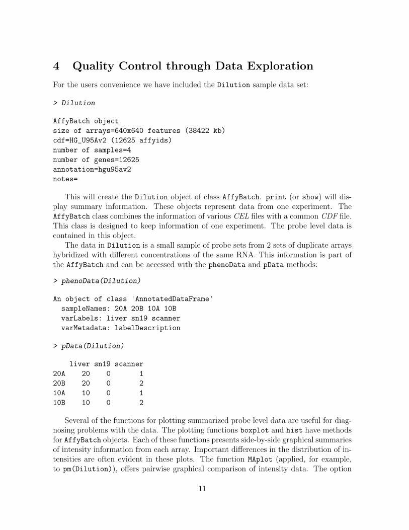
For the users convenience we have included the Dilution sample data set:

> Dilution

AffyBatch object

size of arrays=640x640 features (38422 kb)

cdf=HG_U95Av2 (12625 affyids)

number of samples=4

number of genes=12625

annotation=hgu95av2

notes=

This will create the Dilution object of class AffyBatch. print (or show) will dis-play summary information. These objects represent data from one experiment. TheAffyBatch class combines the information of various CEL files with a common CDF file.This class is designed to keep information of one experiment. The probe level data iscontained in this object.

The data in Dilution is a small sample of probe sets from 2 sets of duplicate arrayshybridized with different concentrations of the same RNA. This information is part ofthe AffyBatch and can be accessed with the phenoData and pData methods:

> phenoData(Dilution)

An object of class 'AnnotatedDataFrame'

sampleNames: 20A 20B 10A 10B

varLabels: liver sn19 scanner

varMetadata: labelDescription

> pData(Dilution)

liver sn19 scanner

20A 20 0 1

20B 20 0 2

10A 10 0 1

10B 10 0 2

Several of the functions for plotting summarized probe level data are useful for diag-nosing problems with the data. The plotting functions boxplot and hist have methodsfor AffyBatch objects. Each of these functions presents side-by-side graphical summariesof intensity information from each array. Important differences in the distribution of in-tensities are often evident in these plots. The function MAplot (applied, for example,to pm(Dilution)), offers pairwise graphical comparison of intensity data. The option

11

pairs permits you to chose between all pairwise comparisons (when TRUE) or comparedto a reference array (the default). These plots can be particularly useful in diagnosingproblems in replicate sets of arrays. The function argument plot.method can be usedto create a MAplot using a smoothScatter, rather than the default method which is todraw every point.

> data(Dilution)

> MAplot(Dilution,pairs=TRUE,plot.method="smoothScatter")

20A

6 8 10 12 14

−2

02

46

Median: 0.59IQR: 0.219

6 8 10 12 14−

20

24

6

Median: 0.329IQR: 0.245

6 8 10 12 14

−4

02

46

Median: 0.989IQR: 0.286

20B

6 8 10 12 14

−3

−1

12

Median: −0.25IQR: 0.244

6 8 10 12−

4−

20

2

Median: 0.415IQR: 0.267

10A

6 8 10 12 14

−4

−2

02

4

Median: 0.653IQR: 0.218

10B

A

M

MVA plot

Figure 3: Pairwise MA plots

4.1 Accessing PM and MM Data

The PM and MM intensities and corresponding affyID can be accessed with the pm, mm,and probeNames methods. These will be matrices with rows representing probe pairs

12

and columns representing arrays. The gene name associated with the probe pair in rowi can be found in the ith entry of the vector returned by probeNames.

> Index <- c(1,2,3,100,1000,2000) ##6 arbitrary probe positions

> pm(Dilution)[Index,]

20A 20B 10A 10B

358160 468.8 282.3 433.0 198.0

118945 430.0 265.0 308.5 192.8

323731 182.3 115.0 138.0 86.3

281340 264.0 151.0 167.0 103.3

361988 152.3 113.0 135.0 88.8

310732 275.0 155.5 194.3 124.5

> mm(Dilution)[Index,]

20A 20B 10A 10B

358800 1123.5 673.0 693.5 434.5

119585 259.0 175.3 194.0 110.3

324371 160.0 95.0 119.3 72.5

281980 180.3 102.5 109.0 74.0

362628 178.8 126.8 156.3 83.5

311372 478.0 284.0 305.0 212.3

> probeNames(Dilution)[Index]

[1] "1000_at" "1000_at" "1000_at" "1006_at" "1057_at" "1114_at"

Index contains six arbitrary probe positions.Notice that the column names of PM and MM matrices are the sample names and

the row names are the affyID, e.g. 1001_at and 1000_at together with the probe number(related to position in the target sequence).

> sampleNames(Dilution)

[1] "20A" "20B" "10A" "10B"

Quick example: To see what percentage of the MM are larger than the PM simplytype

> mean(mm(Dilution)>pm(Dilution))

[1] 0.2746048

The pm and mm functions can be used to extract specific probe set intensities.

13

> gn <- geneNames(Dilution)

> pm(Dilution, gn[100])

20A 20B 10A 10B

1090_f_at1 115.0 74.0 94.0 61.0

1090_f_at2 129.3 80.3 108.0 70.3

1090_f_at3 152.3 81.0 97.5 67.5

1090_f_at4 105.3 76.3 100.3 62.3

1090_f_at5 153.0 111.5 118.0 76.3

1090_f_at6 1984.3 1207.0 1331.3 728.0

1090_f_at7 290.5 181.0 220.0 134.3

1090_f_at8 882.3 532.0 525.0 347.0

1090_f_at9 157.3 105.3 125.0 69.3

1090_f_at10 103.5 83.0 90.0 67.0

1090_f_at11 100.0 75.5 89.0 71.0

1090_f_at12 143.5 92.8 104.3 78.0

1090_f_at13 111.0 70.8 97.0 60.5

1090_f_at14 381.5 255.0 289.0 198.0

1090_f_at15 650.0 389.3 415.0 275.0

1090_f_at16 262.0 157.0 194.8 131.5

The method geneNames extracts the unique affyIDs. Also notice that the 100th probeset is different from the 100th probe! The 100th probe is not part of the the 100th probeset.

The methods boxplot, hist, and image are useful for quality control. Figure 4 showskernel density estimates (rather than histograms) of PM intensities for the 1st and 2ndarray of the Dilution also included in the package.

4.2 Histograms, Images, and Boxplots

As seen in the previous example, the sub-setting method [ can be used to extractspecific arrays. NOTE: Sub-setting is different in this version. One can nolonger subset by gene. We can only define subsets by one dimension: thecolumns, i.e. the arrays. Because the Cel class is no longer available [[ is nolonger available.

The method image() can be used to detect spatial artifacts. By default we look atlog transformed intensities. This can be changed through the transfo argument.

> par(mfrow=c(2,2))

> image(Dilution)

These images are quite useful for quality control. We recommend examining theseimages as a first step in data exploration.

The method boxplot can be used to show PM , MM or both intensities. As discussedin the next section this plot shows that we need to normalize these arrays.

14

> hist(Dilution[,1:2]) ##PM histogram of arrays 1 and 2

6 8 10 12 14

0.0

0.1

0.2

0.3

0.4

0.5

log intensity

dens

ity

Figure 4: Histogram of PM intensities for 1st and 2nd array

15

Figure 5: Image of the log intensities.

16

> par(mfrow=c(1,1))

> boxplot(Dilution, col=c(2,3,4))

X20A X20B X10A X10B

68

1012

14

Small part of dilution study

Figure 6: Boxplot of arrays in Dilution data.

17

4.3 RNA degradation plots

The functions AffyRNAdeg, summaryAffyRNAdeg, and plotAffyRNAdeg aid in assessmentof RNA quality. Individual probes in a probeset are ordered by location relative tothe 5′ end of the targeted RNA molecule.Affymetrix (1999) Since RNA degradationtypically starts from the 5′ end of the molecule, we would expect probe intensities to besystematically lowered at that end of a probeset when compared to the 3′ end. On eachchip, probe intensities are averaged by location in probeset, with the average taken overprobesets. The function plotAffyRNAdeg produces a side-by-side plots of these means,making it easy to notice any 5′ to 3′ trend. The function summaryAffyRNAdeg producesa single summary statistic for each array in the batch, offering a convenient measure ofthe severity of degradation and significance level. For an example

> deg <- AffyRNAdeg(Dilution)

> names(deg)

[1] "N" "sample.names" "means.by.number" "ses"

[5] "slope" "pvalue"

does the degradation analysis and returns a list with various components. A summarycan be obtained using

> summaryAffyRNAdeg(deg)

20A 20B 10A 10B

slope -0.0239 0.0363 0.0273 0.0849

pvalue 0.8920 0.8400 0.8750 0.6160

Finally a plot can be created using plotAffyRNAdeg, see Figure 7.

18

> plotAffyRNAdeg(deg)

RNA degradation plot

5' <−−−−−> 3' Probe Number

Mea

n In

tens

ity :

shift

ed a

nd s

cale

d

0 5 10 15

05

10

Figure 7: Side-by-side plot produced by plotAffyRNAdeg.

19

5 Normalization

Various researchers have pointed out the need for normalization of Affymetrix arrays.See for example Bolstad et al. (2003). The method normalize lets one normalize at theprobe level

> Dilution.normalized <- normalize(Dilution)

For an extended example on normalization please refer to the vignette in the affydatapackage.

6 Classes

AffyBatch is the main class in this package. There are three other auxiliary classes thatwe also describe in this Section.

6.1 AffyBatch

The AffyBatch class has slots to keep all the probe level information for a batch ofCel files, which usually represent an experiment. It also stores phenotypic and MIAMEinformation as does the ExpressionSet class in the Biobase package (the base packagefor BioConductor). In fact, AffyBatch extends ExpressionSet.

The expression matrix in AffyBatch has columns representing the intensities readfrom the different arrays. The rows represent the cel intensities for all position on thearray. The cel intensity with physical coordinates3 (x, y) will be in row

i = x + nrow× (y − 1)

. The ncol and nrow slots contain the physical rows of the array. Notice that thisis different from the dimensions of the expression matrix. The number of row of theexpression matrix is equal to ncol×nrow. We advice the use of the functions xy2indicesand indices2xy to shuttle from X/Y coordinates to indices.

For compatibility with previous versions the accessor method intensity exists forobtaining the expression matrix.

The cdfName slot contains the necessary information for the package to find thelocations of the probes for each probe set. See Section 7 for more on this.

3Note that in the .CEL files the indexing starts at zero while it starts at 1 in the package (as indexingstarts at 1 in R).

20

6.2 ProbeSet

The ProbeSet class holds the information of all the probes related to an affyID. Thecomponents are pm and mm.

The method probeset extracts probe sets from AffyBatch objects. It takes asarguments an AffyBatch object and a vector of affyIDs and returns a list of objects ofclass ProbeSet

> gn <- featureNames(Dilution)

> ps <- probeset(Dilution, gn[1:2])

> #this is what i should be using: ps

> show(ps[[1]])

ProbeSet object:

id=1000_at

pm= 16 probes x 4 chips

The pm and mm methods can be used to extract these matrices (see below).This function is general in the way it defines a probe set. The default is to use

the definition of a probe set given by Affymetrix in the CDF file. However, the usercan define arbitrary probe sets. The argument locations lets the user decide the rownumbers in the intensity that define a probe set. For example, if we are interested inredefining the AB000114_at and AB000115_at probe sets, we could do the following:

First, define the locations of the PM and MM on the array of the 1000_at and1001_at probe sets

> mylocation <- list("1000_at"=cbind(pm=c(1,2,3),mm=c(4,5,6)),

+ "1001_at"=cbind(pm=c(4,5,6),mm=c(1,2,3)))

The first column of the matrix defines the location of the PMs and the second columnthe MMs.

Now we are ready to extract the ProbSets using the probeset function:

> ps <- probeset(Dilution, genenames=c("1000_at","1001_at"),

+ locations=mylocation)

Now, ps is list of ProbeSets. We can see the PMs and MMs of each component usingthe pm and mm accessor methods.

> pm(ps[[1]])

20A 20B 10A 10B

1 149.0 112.0 129.0 60.0

2 1153.5 575.3 1262.3 564.8

3 142.0 98.0 128.0 56.0

21

> mm(ps[[1]])

20A 20B 10A 10B

4 1051 597 1269 570

5 91 77 90 46

6 136 133 117 62

> pm(ps[[2]])

20A 20B 10A 10B

4 1051 597 1269 570

5 91 77 90 46

6 136 133 117 62

> mm(ps[[2]])

20A 20B 10A 10B

1 149.0 112.0 129.0 60.0

2 1153.5 575.3 1262.3 564.8

3 142.0 98.0 128.0 56.0

This can be useful in situations where the user wants to determine if leaving outcertain probes improves performance at the expression level. It can also be useful tocombine probes from different human chips, for example by considering only probescommon to both arrays.

Users can also define their own environment for probe set location mapping. Moreon this in Section 7.

An example of a ProbeSet is included in the package. A spike-in data set is includedin the package in the form of a list of ProbeSets. The help file describes the data set.Figure 8 uses this data set to demonstrate that the MM also detect transcript signal.

7 Location to ProbeSet Mapping

On Affymetrix GeneChip arrays, several probes are used to represent genes in the formof probe sets. From a CEL file we get for each physical location, or cel, (defined by xand y coordinates) an intensity. The CEL file also contains the name of the CDF fileneeded for the location-probe-set mapping. The CDF files store the probe set relatedto each location on the array. The computation of a summary expression values fromthe probe intensities requires a fast way to map an affyid to corresponding probes. Westore this mapping information in R environments4. They only contain a part of theinformation that can be found in the CDF files. The cdfenvs are sufficient to perform

4Please refer to the R documentation to know more about environments.

22

> data(SpikeIn) ##SpikeIn is a ProbeSets

> pms <- pm(SpikeIn)

> mms <- mm(SpikeIn)

> ##pms follow concentration

> par(mfrow=c(1,2))

> concentrations <- matrix(as.numeric(sampleNames(SpikeIn)),20,12,byrow=TRUE)

> matplot(concentrations,pms,log="xy",main="PM",ylim=c(30,20000))

> lines(concentrations[1,],apply(pms,2,mean),lwd=3)

> ##so do mms

> matplot(concentrations,mms,log="xy",main="MM",ylim=c(30,20000))

> lines(concentrations[1,],apply(mms,2,mean),lwd=3)

11

1

1

1111111

111

111

11

1

0.5 2.0 10.0 100.0

5010

050

020

0050

0020

000

PM

concentrations

pms

22

2

2

2222222222

222

222

33

3

3

33

333

33

333

3

3

3

33

3

44

4

4

44

4

44

44444

44

4

44

4

55

5

5

55

5

55

55

555

5

5

5

55

5 66

6

6

66

6

66

66

666

6

6

6

66

677

7

7

77

7

77

77

7

77

7

7

7

77

7

8

8

8

8

88

8

88

88

888

8

8

8

88

899

9

9

99

9

99

99

999

9

9

9

99

9

0

0

0

0

000

00

00

0

00

0

0

0

00

0

a

a

a

a

aaaaa

aa

a

aa

a

a

a

a

a

abb

b

b

bbbbb

bb

bbb

b

b

b

bb

b

11

1

1

1

1

111

1

1

111

1

1

11

1

1

0.5 2.0 10.0 100.0

5010

050

020

0050

0020

000

MM

concentrations

mm

s

22

2

2

2

22222

2

2222

2

222

2

33

3

3

3

3

3

333

3

3333

3

333

3

44

4

4

4

4

4

444

4

4444

4

444

4

55

5

5

5

5

5

55

5

5

5555

5

555

5

66

6

6

6

6

6

66

6

6

6666

6

6

66

6

7

7

7

7

7

7

7

77

7

7

7777

7

7

77

7

8

8

8

8

88

8

88

8

8

8888

8

8

88

8

9

9

9

9

99

9

99

9

9

9

999

9

9

9

9

9

0

0

0

0

00

0

00

0

0

0

000

00

0

0

0

a

a

a

a

aa

a

aa

a

a

a

aaaaa

a

a

a

b

b

b

b

bb

b

bb

b

b

b

bbbb

b

b

b

b

Figure 8: PM and MM intensities plotted against SpikeIn concentration

23

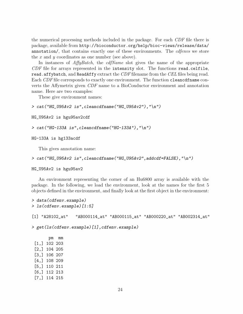
the numerical processing methods included in the package. For each CDF file there ispackage, available from http://bioconductor.org/help/bioc-views/release/data/

annotation/, that contains exactly one of these environments. The cdfenvs we storethe x and y coordinates as one number (see above).

In instances of AffyBatch, the cdfName slot gives the name of the appropriateCDF file for arrays represented in the intensity slot. The functions read.celfile,read.affybatch, and ReadAffy extract the CDF filename from the CEL files being read.Each CDF file corresponds to exactly one environment. The function cleancdfname con-verts the Affymetrix given CDF name to a BioConductor environment and annotationname. Here are two examples:

These give environment names:

> cat("HG_U95Av2 is",cleancdfname("HG_U95Av2"),"\n")

HG_U95Av2 is hgu95av2cdf

> cat("HG-133A is",cleancdfname("HG-133A"),"\n")

HG-133A is hg133acdf

This gives annotation name:

> cat("HG_U95Av2 is",cleancdfname("HG_U95Av2",addcdf=FALSE),"\n")

HG_U95Av2 is hgu95av2

An environment representing the corner of an Hu6800 array is available with thepackage. In the following, we load the environment, look at the names for the first 5objects defined in the environment, and finally look at the first object in the environment:

> data(cdfenv.example)

> ls(cdfenv.example)[1:5]

[1] "A28102_at" "AB000114_at" "AB000115_at" "AB000220_at" "AB002314_at"

> get(ls(cdfenv.example)[1],cdfenv.example)

pm mm

[1,] 102 203

[2,] 104 205

[3,] 106 207

[4,] 108 209

[5,] 110 211

[6,] 112 213

[7,] 114 215

24

[8,] 116 217

[9,] 118 219

[10,] 120 221

[11,] 122 223

[12,] 124 225

[13,] 126 227

[14,] 128 229

[15,] 130 231

[16,] 132 233

The package needs to know what locations correspond to which probe sets. ThecdfName slot contains the necessary information to find the environment with this lo-cation information. The method getCdfInfo takes as an argument an AffyBatch andreturns the necessary environment. If x is an AffyBatch, this function will look for anenvironment with name cleancdfname(x@cdfName).

> print(Dilution@cdfName)

[1] "HG_U95Av2"

> myenv <- getCdfInfo(Dilution)

> ls(myenv)[1:5]

[1] "1000_at" "1001_at" "1002_f_at" "1003_s_at" "1004_at"

By default we search for the environment first in the global environment, then in apackage named cleancdfname(x@cdfName).

Various methods exist to obtain locations of probes as demonstrated in the followingexamples:

> Index <- pmindex(Dilution)

> names(Index)[1:2]

[1] "1000_at" "1001_at"

> Index[1:2]

$`1000_at`

[1] 358160 118945 323731 223978 313420 349209 199525 213669 236739 298099

[11] 282744 281443 349198 297953 317054 404069

$`1001_at`

[1] 340142 236569 327449 203508 300798 276193 354374 400320 250783 379851

[11] 365637 144611 120239 189384 182903 299352

25

pmindex returns a list with probe set names as names and locations in the components.We can also get specific probe sets:

> pmindex(Dilution, genenames=c("1000_at","1001_at"))

$`1000_at`

[1] 358160 118945 323731 223978 313420 349209 199525 213669 236739 298099

[11] 282744 281443 349198 297953 317054 404069

$`1001_at`

[1] 340142 236569 327449 203508 300798 276193 354374 400320 250783 379851

[11] 365637 144611 120239 189384 182903 299352

The locations are ordered from 5’ to 3’ on the target transcript. The function mmindex

performs in a similar way:

> mmindex(Dilution, genenames=c("1000_at","1001_at"))

$`1000_at`

[1] 358800 119585 324371 224618 314060 349849 200165 214309 237379 298739

[11] 283384 282083 349838 298593 317694 404709

$`1001_at`

[1] 340782 237209 328089 204148 301438 276833 355014 400960 251423 380491

[11] 366277 145251 120879 190024 183543 299992

They both use the method indexProbes

> indexProbes(Dilution, which="pm")[1]

$`1000_at`

[1] 358160 118945 323731 223978 313420 349209 199525 213669 236739 298099

[11] 282744 281443 349198 297953 317054 404069

> indexProbes(Dilution, which="mm")[1]

$`1000_at`

[1] 358800 119585 324371 224618 314060 349849 200165 214309 237379 298739

[11] 283384 282083 349838 298593 317694 404709

> indexProbes(Dilution, which="both")[1]

$`1000_at`

[1] 358160 118945 323731 223978 313420 349209 199525 213669 236739 298099

[11] 282744 281443 349198 297953 317054 404069 358800 119585 324371 224618

[21] 314060 349849 200165 214309 237379 298739 283384 282083 349838 298593

[31] 317694 404709

The which="both" options returns the location of the PMs followed by the MMs.

26

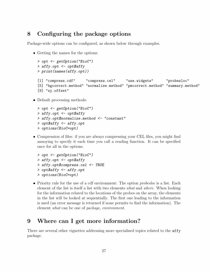
8 Configuring the package options

Package-wide options can be configured, as shown below through examples.

� Getting the names for the options:

> opt <- getOption("BioC")

> affy.opt <- opt$affy

> print(names(affy.opt))

[1] "compress.cdf" "compress.cel" "use.widgets" "probesloc"

[5] "bgcorrect.method" "normalize.method" "pmcorrect.method" "summary.method"

[9] "xy.offset"

� Default processing methods:

> opt <- getOption("BioC")

> affy.opt <- opt$affy

> affy.opt$normalize.method <- "constant"

> opt$affy <- affy.opt

> options(BioC=opt)

� Compression of files: if you are always compressing your CEL files, you might findannoying to specify it each time you call a reading function. It can be specifiedonce for all in the options.

> opt <- getOption("BioC")

> affy.opt <- opt$affy

> affy.opt$compress.cel <- TRUE

> opt$affy <- affy.opt

> options(BioC=opt)

� Priority rule for the use of a cdf environment: The option probesloc is a list. Eachelement of the list is itself a list with two elements what and where. When lookingfor the information related to the locations of the probes on the array, the elementsin the list will be looked at sequentially. The first one leading to the informationis used (an error message is returned if none permits to find the information). Theelement what can be one of package, environment.

9 Where can I get more information?

There are several other vignettes addressing more specialised topics related to the affy

package.

27

� affy: Custom Processing Methods (HowTo): A description of how to usecustom preprocessing methods with the package. This document gives examples ofhow you might write your own preprocessing method and use it with the package.

� affy: Built-in Processing Methods: A document giving fuller descriptions ofeach of the preprocessing methods that are available within the affy package.

� affy: Import Methods (HowTo): A discussion of the data structures used andhow you might import non standard data into the package.

� affy: Loading Affymetrix Data (HowTo): A quick guide to loading Affymetrixdata into R.

� affy: Automatic downloading of cdfenvs (HowTo): How you can configurethe automatic downloading of the appropriate cdfenv for your analysis.

A Previous Release Notes

A.1 Changes in versions 1.6.x

There were very few changes.

� The function MAplot has been added. It works on instances of AffyBatch. Youcan decide if you want to make all pairwise MA plots or compare to a referencearray using the pairs argument.

� Minor bugs fixed in the parsers.

� The path of celfiles is now removed by ReadAffy.

A.2 Changes in versions 1.5.x

There are some minor differences in what you can do but little functionality has disap-peared. Memory efficiency and speed have improved.

� The widgets used by ReadAffy have changed.

� The path of celfiles is now removed by ReadAffy.

A.3 Changes in versions 1.4.x

There are some minor differences in what you can do but little functionality has disap-peared. Memory efficiency and speed have improved.

28

� For instances of AffyBatch the subsetting has changed. For consistency withexprSets one can only subset by the second dimension. So to obtain the firstarray, abatch[1] and abatch[1,] will give warnings (errors in the next release).The correct code is abatch[,1].

� mas5calls is now faster and reproduces Affymetrix’s official version much better.

� If you use pm and mm to get the entire set of probes, e.g. by typing pm(abatch)

then the method will be, on average, about 2-3 times faster than in version 1.3.

References

Affymetrix. Affymetrix Microarray Suite User Guide. Affymetrix, Santa Clara, CA,version 4 edition, 1999.

Affymetrix. Affymetrix Microarray Suite User Guide. Affymetrix, Santa Clara, CA,version 5 edition, 2001.

B.M. Bolstad, R.A. Irizarry, M. Astrand, and T.P. Speed. A comparison of normaliza-tion methods for high density oligonucleotide array data based on variance and bias.Bioinformatics, 19(2):185–193, Jan 2003.

Laurent Gautier, Leslie Cope, Benjamin Milo Bolstad, and Rafael A. Irizarry. affy - an rpackage for the analysis of affymetrix genechip data at the probe level. Bioinformatics,2003. In press.

Rafael A. Irizarry, Laurent Gautier, and Leslie M. Cope. The Analysis of Gene Expres-sion Data: Nethods and Software, chapter 4. Spriger Verlag, 2003a.

Rafael A. Irizarry, Bridget Hobbs, Francois Collin, Yasmin D. Beazer-Barclay, Kristen J.Antonellis, Uwe Scherf, and Terence P. Speed. Exploration, normalization, and sum-maries of high density oligonucleotide array probe level data. Biostatistics, 2003b. Toappear.

C. Li and W.H. Wong. Model-based analysis of oligonucleotide arrays: Expression indexcomputation and outlier detection. Proceedings of the National Academy of ScienceU S A, 98:31–36, 2001.

29