dermal radiomics: a new approach for computer-aided

Dermal Radiomics: A New Approach

For Computer-Aided Melanoma

Screening System

by

Sungjoon Cho

A thesis

presented to the University of Waterloo

in fulfillment of the

thesis requirement for the degree of

Doctor of Philosophy

in

Systems Design Engineering

Waterloo, Ontario, Canada, 2016

c© Sungjoon Cho 2016

This thesis consists of material all of which I authored or co-authored: see Statement

of Contributions included in the thesis. This is a true copy of the thesis, including any

required final revisions, as accepted by my examiners.

I understand that my thesis may be made electronically available to the public.

ii

Statement of Contributions

The following four papers are used in this thesis. They are described below:

D. S. Cho, S. Haider, R. Amelard, A. Wong, and D. A. Clausi : Physiological Charac-

terization of Skin Lesion using Non-linear Random Forest Regression Model. 36th Annual

International IEEE Engineering in Medicine and Biology Society Conference (EMBC),

Chicago, IL, USA, pp. 6455-6458, 2014

This paper is incorporated in Chapter 3 of this thesis.

Contributor Statement of Contribution

D. S. Cho (Candidate) Conceptual design (60%)

Data collection and analysis (60%)

Writing and editing (60%)

S. Haider Data collection and analysis (30%)


R. Amelard Conceptual design (10%)


A. Wong Conceptual design (20%)



D. A. Clausi Conceptual design (10%)


iii

D. S. Cho, S. Haider, R. Amelard, A. Wong, and D. A. Clausi : Quantitative Fea-

tures For Computer-Aided Melanoma Classification Using Spatial Heterogeneity Of Eume-

lanin And Pheomelanin Concentrations. International Symposium on Biomedical Imaging

(ISBI), 2015 IEEE 12th International Symposium on. IEEE, 2015






S. Haider Data collection and analysis (20%)


R. Amelard Conceptual design (20%)







iv

D. S. Cho, D. A. Clausi, and A. Wong : Dermal Radiomics for Melanoma Screening,

Vision Letters 1.1, 2015











v

D. S. Cho, D. A. Clausi, and A. Wong : Accuracy of Melanoma Classification using

Dermal Radiomic Sequences. Imaging Network Ontario 14th Annual Symposium, Toronto,

ON, CANADA, February, 2016











vi

Abstract

Skin cancer is the most common form of cancer in North America, and melanoma

is the most dangerous type of skin cancer. Melanoma originates from melanocytes in

the epidermis and has a high tendency to develop away from the skin surface and cause

metastasis through the bloodstream. Early diagnosis is known to help improve survival

rates. Under the current diagnosis, the initial examination of the potential melanoma

patient is done via naked eye screening or standard photographic images of the lesion.

From this, the accuracy of diagnosis varies depending on the expertise of the clinician.

Radiomics is a recent cancer diagnostic tool that centers around the high throughput

extraction of quantitative and mineable imaging features from medical images to identify

tumor phenotypes. Radiomics focuses on optimizing a large number of features through

computational approaches to develop a decision support system for improving individu-

alized treatment selection and monitoring. While radiomics has shown great promise for

screening and analyzing different forms of cancer such as lung cancer and prostate cancer,

to the best of our knowledge, radiomics has not been previously adopted for skin cancer,

especially melanoma.

This work presents a dermal radiomics framework, which is a novel computer-aided

melanoma diagnosis. While most computer-aided melanoma screening systems follow the

conventional diagnostic scheme, the proposed work utilizes the physiological biomarker

information. To extract physiological biomarkers, non-linear random forest inverse light-

skin interaction model is proposed. The construction of dermal radiomics sequence is

followed using the extracted physiological biomarkers, and the dermal radiomics framework

for melanoma is completed by constructing diagnostic decision system based on random

forest classification algorithm.

vii

Acknowledgements

First, I would like to thank my two co-supervisors, professor David Clausi and Alexan-

der Wong. For the last four years, I had ups and downs on my research. Whenever I

struggle, you are always there for the encouragement and guidance and got my back. It

has been such a blessing to have you as my supervisors.

I would also like to express my gratitude to my Ph.D committee members, Dr. John

Zelek, and Dr. Stacey Scott from the department of Systems Design Engineering, Dr.

Justin Wan from the department of Computer Science, and Dr. Kostadinka Bizheva from

the department of Physics and Astronomy for your advice.

To all members from the Vision and Imaging Processing lab, you guys made my lab

life fun and sweet (with a bunch of brownies, cupcakes, cookies, and much more!).

I would sincerely like to thank my family with all of their love and support. To my

parents, and my parents-in-law, you have been my rock and shelter. Without you, I would

not be able to come this far. Thank you. To my sons, Jayden, and Caleb, you are always

joy and ’turbo-boost’ in my life. To my wife Annie, the words cannot express how much I

thank you. You have always been my helping hand.

Last but not least, to my father in heaven, who has given me the strength and wisdom

to finish my thesis. Thank you for being my provider.

viii

Table of Contents

List of Tables xiv

List of Figures xv

1 Introduction 1

1.1 Melanoma . . . . . . . . . . . . . . . . . . . . . . . . . . . . . . . . . . . . 1

1.2 Radiomics . . . . . . . . . . . . . . . . . . . . . . . . . . . . . . . . . . . . 2

1.3 Radiomics-driven Computer-aided Melanoma Screening System . . . . . . 3

1.4 Motivation . . . . . . . . . . . . . . . . . . . . . . . . . . . . . . . . . . . . 5

1.5 Thesis Contributions . . . . . . . . . . . . . . . . . . . . . . . . . . . . . . 6

2 Overview of Malignant Melanoma 7

2.1 Types of Lesion . . . . . . . . . . . . . . . . . . . . . . . . . . . . . . . . . 7

2.1.1 Benign Lesions . . . . . . . . . . . . . . . . . . . . . . . . . . . . . 7

2.1.2 Non-melanoma Skin Cancer . . . . . . . . . . . . . . . . . . . . . . 8

2.1.3 Melanoma . . . . . . . . . . . . . . . . . . . . . . . . . . . . . . . . 9

2.2 Risk Factors, Staging, and Treatment of Melanoma . . . . . . . . . . . . . 10

2.2.1 Risk Factors . . . . . . . . . . . . . . . . . . . . . . . . . . . . . . . 10

ix

2.2.2 Staging . . . . . . . . . . . . . . . . . . . . . . . . . . . . . . . . . 12

2.2.3 Treatment . . . . . . . . . . . . . . . . . . . . . . . . . . . . . . . . 13

2.3 Diagnosis of Melanoma . . . . . . . . . . . . . . . . . . . . . . . . . . . . . 14

2.3.1 Clinical Examination . . . . . . . . . . . . . . . . . . . . . . . . . . 14

2.3.2 Imaging Techniques for Clinical Examination . . . . . . . . . . . . . 14

2.3.3 Pathological Examination . . . . . . . . . . . . . . . . . . . . . . . 17

2.3.4 The Computer-aided Melanoma Diagnosis . . . . . . . . . . . . . . 17

2.4 Understanding Skin and Physiological Biomarkers . . . . . . . . . . . . . . 18

2.4.1 Structure of Skin . . . . . . . . . . . . . . . . . . . . . . . . . . . . 19

2.4.2 Important Physiological Biomarkers Related to Melanoma . . . . . 20

2.5 Summary . . . . . . . . . . . . . . . . . . . . . . . . . . . . . . . . . . . . 22

3 Physiological Biomarker Extraction Model 23

3.1 Light-skin Interaction Model . . . . . . . . . . . . . . . . . . . . . . . . . . 23

3.2 Existing Models . . . . . . . . . . . . . . . . . . . . . . . . . . . . . . . . . 25

3.2.1 Erythema Index and Melanin Index . . . . . . . . . . . . . . . . . . 25

3.2.2 Linear Light-skin Interaction Modeling . . . . . . . . . . . . . . . . 26

3.2.3 Nearest Neighbor Model . . . . . . . . . . . . . . . . . . . . . . . . 27

3.3 Proposed Random Forest Model . . . . . . . . . . . . . . . . . . . . . . . . 28

3.3.1 Non-linear, Forward Light-skin Interaction Model . . . . . . . . . . 28

3.3.2 Non-linear Random Forest Inverse Light-skin Interaction Model . . 32

3.4 Summary . . . . . . . . . . . . . . . . . . . . . . . . . . . . . . . . . . . . 37

x

4 Experimental Results For Physiological Biomarker Extraction 38

4.1 Testing Algorithms . . . . . . . . . . . . . . . . . . . . . . . . . . . . . . . 38

4.1.1 Linear Light-skin Interaction Modeling . . . . . . . . . . . . . . . . 39

4.1.2 Cavalcanti’s Nearest Neighbor Model . . . . . . . . . . . . . . . . . 39

4.1.3 Ensemble Techniques . . . . . . . . . . . . . . . . . . . . . . . . . . 40

4.2 Experimental Design . . . . . . . . . . . . . . . . . . . . . . . . . . . . . . 41

4.2.1 Cross Validation . . . . . . . . . . . . . . . . . . . . . . . . . . . . 42

4.2.2 Skin Lesion Simulation Study . . . . . . . . . . . . . . . . . . . . . 42

4.2.3 Clinical Validation . . . . . . . . . . . . . . . . . . . . . . . . . . . 44

4.3 Discussion . . . . . . . . . . . . . . . . . . . . . . . . . . . . . . . . . . . . 47

4.4 Summary . . . . . . . . . . . . . . . . . . . . . . . . . . . . . . . . . . . . 49

5 Dermal Radiomics Sequence 50

5.1 Introduction . . . . . . . . . . . . . . . . . . . . . . . . . . . . . . . . . . . 50

5.2 Existing Dermal Radiomics Feature Set . . . . . . . . . . . . . . . . . . . . 51

5.2.1 Low Level Feature . . . . . . . . . . . . . . . . . . . . . . . . . . . 51

5.2.2 High-level Intuitive Feature . . . . . . . . . . . . . . . . . . . . . . 53

5.3 Proposed Dermal Radiomics Feature Set . . . . . . . . . . . . . . . . . . . 54

5.3.1 Physiological Feature . . . . . . . . . . . . . . . . . . . . . . . . . . 54

5.3.2 Physiological Texture Feature . . . . . . . . . . . . . . . . . . . . . 58

5.4 Generating Dermal Radiomics Sequence . . . . . . . . . . . . . . . . . . . 60

5.5 Experimental Setup . . . . . . . . . . . . . . . . . . . . . . . . . . . . . . . 60

5.5.1 Data . . . . . . . . . . . . . . . . . . . . . . . . . . . . . . . . . . . 61

5.5.2 Pre-processing . . . . . . . . . . . . . . . . . . . . . . . . . . . . . . 61

xi

5.5.3 Classification . . . . . . . . . . . . . . . . . . . . . . . . . . . . . . 62

5.5.4 Validation Study on Proposed Physiological Feature Sets . . . . . . 63

5.5.5 Validation Study on Dermal Radiomics Sequence . . . . . . . . . . 64

5.5.6 Results . . . . . . . . . . . . . . . . . . . . . . . . . . . . . . . . . . 65

5.6 Summary . . . . . . . . . . . . . . . . . . . . . . . . . . . . . . . . . . . . 68

6 Feature Analysis for Dermal Radiomics 69

6.1 Introduction . . . . . . . . . . . . . . . . . . . . . . . . . . . . . . . . . . . 69

6.2 Classification Analysis . . . . . . . . . . . . . . . . . . . . . . . . . . . . . 69

6.2.1 Experimental Design . . . . . . . . . . . . . . . . . . . . . . . . . . 70

6.2.2 Results . . . . . . . . . . . . . . . . . . . . . . . . . . . . . . . . . . 71

6.2.3 Parametrization of Random Forest Classification . . . . . . . . . . . 72

6.3 Feature Selection Analysis . . . . . . . . . . . . . . . . . . . . . . . . . . . 75

6.3.1 ReliefF . . . . . . . . . . . . . . . . . . . . . . . . . . . . . . . . . . 75

6.3.2 Random forest variable importance (RF-VI) . . . . . . . . . . . . . 76

6.3.3 Maximum Relevance, Minimum Redundancy Technique . . . . . . . 77

6.3.4 Experimental Design . . . . . . . . . . . . . . . . . . . . . . . . . . 77

6.3.5 Results . . . . . . . . . . . . . . . . . . . . . . . . . . . . . . . . . . 79

6.4 Validation study on dermal radiomics . . . . . . . . . . . . . . . . . . . . . 82

6.4.1 Comparison with the state-of-the-art techniques . . . . . . . . . . . 82

6.4.2 Comparison with conventional diagnosis . . . . . . . . . . . . . . . 84

6.5 Summary . . . . . . . . . . . . . . . . . . . . . . . . . . . . . . . . . . . . 85

7 Conclusions 86

7.1 Summary of Contributions . . . . . . . . . . . . . . . . . . . . . . . . . . . 86

7.2 Future Research . . . . . . . . . . . . . . . . . . . . . . . . . . . . . . . . . 87

xii

References 90

A Colour Space Conversion 107

A.1 XYZ to RGB Conversion . . . . . . . . . . . . . . . . . . . . . . . . . . . . 107

A.2 XYZ to L*a*b* Conversion . . . . . . . . . . . . . . . . . . . . . . . . . . 108

A.3 XYZ to L*u*v* . . . . . . . . . . . . . . . . . . . . . . . . . . . . . . . . . 108

A.4 XYZ to xyz . . . . . . . . . . . . . . . . . . . . . . . . . . . . . . . . . . . 109

A.5 RGB to rgb . . . . . . . . . . . . . . . . . . . . . . . . . . . . . . . . . . . 109

xiii

List of Tables

4.1 Comparing Fisher separability of eumelanin, pheomelanin and hemoglobin

predicted using RF, NN and AdaBoost (AB). . . . . . . . . . . . . . . . . 47

4.2 Two-sample t-test between the proposed physiological biomarker extraction

technique and the existing extraction methods . . . . . . . . . . . . . . . . 48

6.1 Two-sample t-test between RF classification, SVM and NB. . . . . . . . . 72

6.2 Evaluation results by varying the value of mtry . . . . . . . . . . . . . . . . 74

6.3 Evaluation results by varying the value of ntree . . . . . . . . . . . . . . . . 74

6.4 50 trials of 80/20 cross validation results for classification analysis . . . . . 80

6.5 50 trials of 80/20 cross validation results with feature selection algorithm . 83

6.6 50 trials of 80/20 cross validation results without feature selection algorithm 83

6.7 Two-sample t-test between the dermal radiomics and the state-of-the-art

techniques. . . . . . . . . . . . . . . . . . . . . . . . . . . . . . . . . . . . . 84

xiv

List of Figures

1.1 The radiomics workflow is presented . . . . . . . . . . . . . . . . . . . . . . 2

1.2 The proposed radiomics-driven melanoma screening system is presented. . 4

2.1 Estimated age-standardized incidence and mortality rates in Canada(2015). 9

2.2 Visualization of four subtypes of melanoma and their descriptions. . . . . . 11

2.3 Clinical Examination: Explanation of ABCDE rule. . . . . . . . . . . . . . 15

2.4 Illustration of the skin structure including the epidermis, the papillary der-

mis, and the reticular dermis. . . . . . . . . . . . . . . . . . . . . . . . . . 19

3.1 Illustration of how skin is colourized through light-skin interaction . . . . . 24

3.2 Illustration of the proposed forward model . . . . . . . . . . . . . . . . . . 29

3.3 Visual representation of the original sample set. . . . . . . . . . . . . . . . 35

3.4 Illustration of random forest model which predicts concentration maps of

eumelanin, pheomelanin, and hemoglobin from a skin lesion image . . . . . 36

4.1 10-fold cross validation results for the random forest regression (RF), the

Cavalcanti’s nearest neighbor model (NN), AdaBoost (AB), and bagging(BA).

Error bars indicate the 95% confidence intervals based on the Students T

distribution . . . . . . . . . . . . . . . . . . . . . . . . . . . . . . . . . . . 41

4.2 A simulated image and its ground truth concentrations of physiological

biomarker were presented. . . . . . . . . . . . . . . . . . . . . . . . . . . . 43

xv

4.3 RMSE from the predicted concentrations by RF, NN, AB and BA. Error

bars indicate the 95% confidence intervals based on the Students T distribution 44

4.4 a) Ground truth concentration of eumelanin in a simulated image was pre-

dicted by b) RF, c) NN, d) AB, e) BA, f) MI/EI, and g) MF. . . . . . . . 45

4.5 a) Ground truth concentration of pheomelanin in a simulated image was

predicted by b) RF, c) NN, d) AB, e) BA, and f) MF. . . . . . . . . . . . 45

4.6 a) Ground truth concentration of hemoglobin in a simulated image was

predicted by b) RF, c) NN, d) AB, e) BA, f) MI/EI, and g) MF. . . . . . . 46

5.1 Detailed block diagram of the proposed dermal radiomics sequence. . . . . 51

5.2 A visualization of spatial heterogeneity of physiological biomarkers is pre-

sented. . . . . . . . . . . . . . . . . . . . . . . . . . . . . . . . . . . . . . . 56

5.3 An example skin lesion image with delineated boundaries of outer region(green),

lesion(red), and inner region(blue) . . . . . . . . . . . . . . . . . . . . . . . 57

5.4 An example of concentration maps of physiological biomarkers, which are

extracted from six different colour spaces, is presented. . . . . . . . . . . . 59

5.5 Pre-processing steps are presented. . . . . . . . . . . . . . . . . . . . . . . 62

5.6 Comparing classification results from FA, FB, FC , and FPB over 50 80/20

validation trials. Error bars indicate the 95% confidence intervals based on

the Students T distribution. . . . . . . . . . . . . . . . . . . . . . . . . . . 65

5.7 Comparing classification results from FLLF , FHLIF , FPF , and FDRS over 50

80/20 validation trials. Error bars indicate the 95% confidence intervals

based on the Students T distribution . . . . . . . . . . . . . . . . . . . . . 67

6.1 80/20 cross validation: The sensitivity, specificity, and accuracy of RF,

SVM, and NB classification are reported. Error bars indicate the 95% con-

fidence intervals based on the Students T distribution. . . . . . . . . . . . 71

xvi

6.2 Leave-one-out cross validation: The sensitivity, specificity, and accuracy of

RF, SVM, and NB classification are reported. Error bars indicate the 95%

confidence intervals based on the Students T distribution. . . . . . . . . . . 72

6.3 ROC for RF, SVM, and NB classification . . . . . . . . . . . . . . . . . . . 73

6.4 The sensitivity results of Leave-one-out cross validation using mRMR, Re-

liefF and RF-VI as feature selection algorithms . . . . . . . . . . . . . . . 78

6.5 The specificity results of Leave-one-out cross validation using mRMR, Reli-

efF and RF-VI as feature selection algorithms . . . . . . . . . . . . . . . . 78

6.6 The accuracy results of Leave-one-out cross validation using mRMR, ReliefF

and RF-VI as feature selection algorithms . . . . . . . . . . . . . . . . . . 79

6.7 ROC for different feature selection methods . . . . . . . . . . . . . . . . . 81

xvii

Chapter 1

Introduction

This thesis presents dermal radiomics, which is a new approach of screening and diag-

nosing melanoma with the help of computer system. To construct this dermal radiomics

framework, three items are presented: 1) physiological biomarker extraction, 2) dermal

radiomics sequence construction and 3) feature analysis of dermal radiomics sequence. In

this chapter, we briefly explain each component of dermal radiomics, which are malignant

melanoma and radiomics.

1.1 Melanoma

Melanoma is the most lethal form of skin cancer [63]. In Canada alone, an estimated 6,000

new cases are diagnosed as melanoma each year, and 0.2 million cases worldwide [27, 49].

With an early diagnosis, melanoma can be completely cured with a simple extraction of

the cancerous tissue. However, as melanoma advances into later stages, the cancer can

spread and the prognosis becomes dismal. In North America, melanoma cases are initially

diagnosed by a dermatologist or general practitioner, and confirmed by a pathologist (given

a biopsy by the dermatologist). Furthermore, the initial diagnosis is usually performed with

naked-eye examination for determining suspicious malignant lesions, sometimes with the

aid of a dermoscope [47]. A dermoscope is an optical device used by some dermatologists

1

to magnify skin lesion and to remove skin surface reflection. Even with the help of a

dermoscope, the visual examination may bring difficulties to correctly identify melanoma.

For example, melanoma at early to mid stages is difficult to be distinguished from benign

dysplastic nevi (i.e., moles) by visual inspection. Moreover, melanoma can be observed

in many different shapes and forms, which makes it even more difficult to identify a new

lesion as a melanoma. While identifying melanoma as early as possible is crucial for the

better patient prognosis, accurate diagnosis is still challenging for any physician.

1.2 Radiomics

Medical imaging is conventionally used for the diagnostic purpose to find a potential tumor

and to monitor its’ changes over time. With the advancement in imaging acquisition tech-

nique, medical imaging extends from its primary role to become a non-invasive prognostic

tool by providing objective and precise quantitative imaging descriptors. Radiomics has

recently emerged, and the principle idea of radiomics is to convert imaging data into a

large number of quantitative and mineable imaging features using data-characterization

algorithms [2]. Although each extracted feature may not have any known clinical signifi-

cance, radiomics focuses on optimizing a large number of features through computational

approaches to develop a decision support system for improving individualized treatment

selection and monitoring [91].

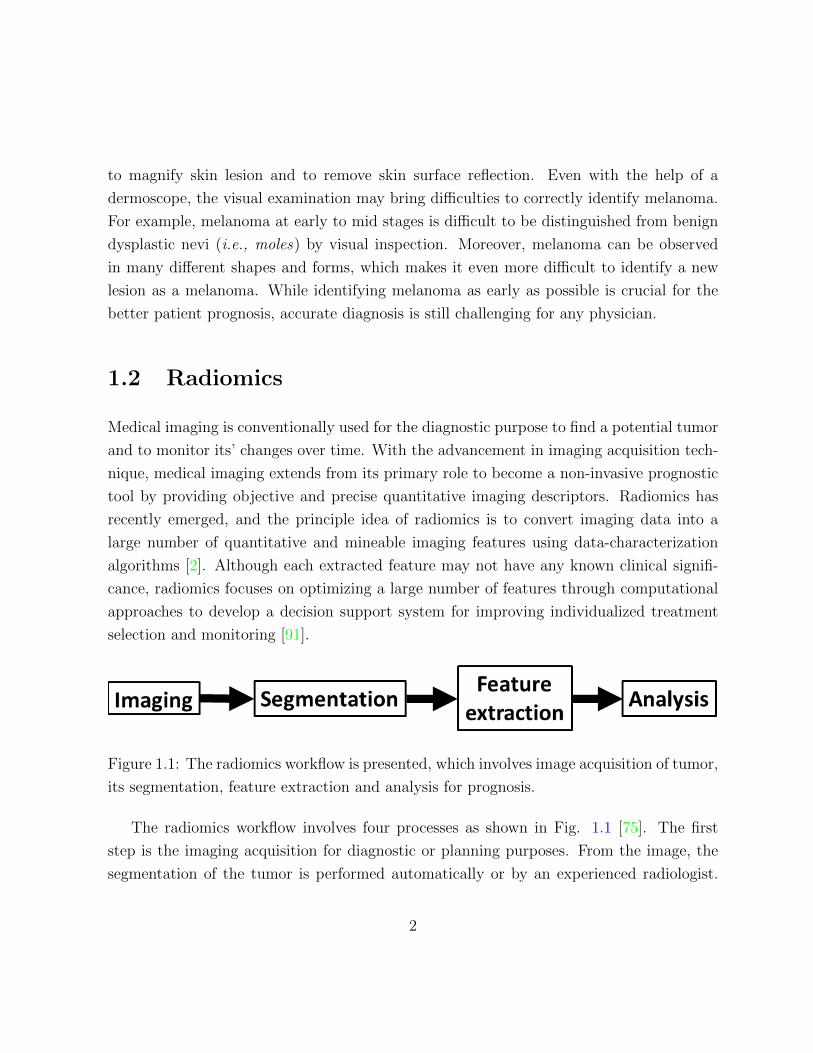
Figure 1.1: The radiomics workflow is presented, which involves image acquisition of tumor,

its segmentation, feature extraction and analysis for prognosis.

The radiomics workflow involves four processes as shown in Fig. 1.1 [75]. The first

step is the imaging acquisition for diagnostic or planning purposes. From the image, the

segmentation of the tumor is performed automatically or by an experienced radiologist.

2

Next, quantitative imaging features are extracted based on the tumor segmentation, and

the feature selection procedure is followed to find the most informative features. The

selected features are then analyzed for their relationship with treatment outcomes.

1.3 Radiomics-driven Computer-aided Melanoma Screen-

ing System

While radiomics has shown great promise for screening and analyzing different forms of

cancer such as lung, head and neck, and prostate cancer [91, 2, 65], to the best of our knowl-

edge, radiomics has not been previously adopted for skin cancer, especially melanoma. As

such, radiomics is expected to have benefits for melanoma screening, especially since clinical

screening currently relies solely on visual assessment of skin lesions.

Therefore, we propose a radiomics-driven computer-aided melanoma screening system,

which is now referred to as dermal radiomics throughout the thesis. The dermal radiomics

framework consists of four processes, and its’ workflow is shown in Fig. 1.2. Imaging

modalities used for dermal radiomics are standard camera images or dermascopic images.

Segmentation is conducted manually and is coupled with an extra pre-processing step.

Pre-processing in dermal radiomics is used to ensure that each image acquired is min-

imized from skin surface reflection and is scale- and rotation- invariant. Segmentation

process will be explained in detail in Section 5.5.2. The next step in radiomics is feature

extraction. In the proposed dermal radiomics, this step is further divided into two as

physiological biomarker extraction and dermal radiomics sequence construction. In physi-

ological biomarker extraction, we extract sub-dermal physiological biomarkers from image

data such as melanin and hemoglobin, which are not typically available to dermatologists

but only to pathologists via a pathological report. Based on the extracted physiological

biomarkers, a dermal radiomics sequence is constructed. Lastly, dermal radiomics em-

ploys classification and feature selection algorithm to analyze the sequence and provide an

accurate diagnosis of a skin lesion.

3

Figure 1.2: The proposed radiomics-driven melanoma screening system is presented.

4

1.4 Motivation

The motivation for developing dermal radiomics can be explained in three ways.

First, as aforementioned, early diagnosis is the key for improving prognosis of patients

with melanoma because melanoma likely penetrates deeper and causes metastasis [8]. Cur-

rent clinical examination primarily relies on the subjectivity of clinicians and dermatol-

ogists, and thus, the diagnosis may be different from one clinician to another depending

on their expertise. Although most dermatologists use the standard diagnostic scheme for

clinical examination, the reported accuracy of diagnosing melanoma with the unaided eye

is only about 60% [67]. Therefore, dermal radiomics can help dermatologists and clini-

cians to make more robust decision using quantitative image features, rather than solely

depending on their training.

Second, even though the clinicians and dermatologists conduct the initial diagnosis, the

diagnosis is confirmed by the pathological report through biopsy. Since the process of pro-

ducing the pathological report through biopsy is time-consuming, expensive and painful, it

is especially challenging for those who have many moles that need to be dissected for biopsy.

Therefore, an accurate initial diagnosis to reduce any unnecessary biopsy is crucial. The

fundamental limitation of the initial diagnosis by visual inspection, is that this only exam-

ines the surface of the lesion, while pathological report investigates sub-dermal pathology.

Given that the melanoma originates from melanocytes, and melanocytes are responsible for

producing melanin, investigating the activities of physiological biomarkers such as melanin

on the suspicious lesion should provide additional knowledge for dermatologists to improve

the accuracy on the diagnosis of the melanoma before biopsy.

Last, dermal radiomics can be used as a tele-medicine tool to find potential malignant

lesions. Under current practice, any abnormal lesions should be confirmed by clinicians

or dermatologists, and many abnormal lesions could be ignored because people do not go

to doctors. Moreover, for those who live in remote area or in an underdeveloped country,

the access to clinicians or dermatologists is not easy. This will inevitably delay the initial

diagnosis as well as the proper treatment in a reasonable time frame to prevent spread of

the cancer. With the proposed dermal radiomics, patients can upload or send a image of

suspicious lesion and get pre-diagnosed for the severity of the lesion. If the screening system

5

identifies a lesion to require immediate attention by clinicians, then they can proceed with

more confidence and improve the diagnosis accuracy for patients.

1.5 Thesis Contributions

The thesis makes following contributions:

• In Chapter 3 and 4, a novel method to extract the concentration of physiological

biomarkers for dermal radiomics is introduced and validated. Most existing tech-

niques for physiological biomarker extraction are based on a linear light-skin inter-

action model, which describes only single light-skin interaction, namely, absorption.

The proposed model uses a non-linear, forward light-skin interaction model, which ac-

counts for various interactions including surface reflection, subsurface scattering, and

absorption between light and physiological biomarkers. From this forward model, a

non-linear random forest inverse light-skin interaction model is constructed to extract

the concentration of eumelanin, pheomelanin, and hemoglobin.

• In Chapter 5, the construction of a dermal radiomics sequence is proposed. While

most computer-aided melanoma screening system use the feature model that simply

quantifies the existing diagnostic scheme (i.e., ABCD-rule), the proposed feature

model generates a large number of features that characterize a skin lesion based

not only on the appearance of the skin lesion but also the activities of physiological

biomarkers.

• In Chapter 6, feature analysis of the dermal radiomics sequence is designed to com-

plete the dermal radiomics framework. The feature analysis process is divided into

classification analysis and feature selection analysis. Through several validation stud-

ies, a feature selection and classification algorithm, that works effectively with the

dermal radiomics sequence, are provided.

6

Chapter 2

Overview of Malignant Melanoma

Skin cancer is the most common form of cancer in North America [104, 27]. This disease

can be categorized into two types depending on its causes: melanoma and non-melanoma.

Melanoma is the most lethal form of skin cancer, and originates from uncontrollable re-

production of melanocytes, which is responsible for producing pigments of skin. Although

non-melanoma skin cancer accounts for the majority of skin cancer cases, more research

focus is aimed at melanoma because non-melanoma skin cancer can be cured with the

proper treatment, while melanoma is more aggressive and becomes incurable as the cancer

progresses[8]. In this chapter, a brief overview of melanoma including risk factors, staging,

and diagnosis is given. Moreover, a overview of skin anatomy relevant to understanding

melanoma and current clinical methods for detecting melanoma is discussed.

2.1 Types of Lesion

2.1.1 Benign Lesions

Benign lesions typically represent any ordinary moles, which rarely cause any harm to hu-

mans, and are subcategorized into two types: melanocytic and non-melanocytic. Melanocytic

lesions develops from melanocytes as the result of excessive production of melanin. Exam-

ples of melanocytic lesions are junctional nevi, compound nevi, intradermal nevi, halo nevi,

7

congenital nevi, acquired nevi, dysplastic nevi, spitz nevi, and blue nevi. Non-melanocytic

lesions are moles that do not arise from melanocytes, and dermatofibromas, haemangiomas,

and seborrheic keratosis are the examples of non-melanocytic lesions. These benign lesions

vary in size, shape and colour, and some of them such as dysplatic nevi and seborrheic

keratosis are often misdiagnosed asmelanoma because of their visual resemblance with

melanoma.

2.1.2 Non-melanoma Skin Cancer

Non-melanoma skin cancer (NMSC) is the most common type of cancer in the Caucasian

population. As the name suggests, NMSC refers all types of skin cancers that are not

malignant melanoma. The major difference between NMSC and melanoma is the origin

of the cancer. While melanoma begins from melanocytes, NMSC originates from other

cells in skin. For example, two main types of NMSC are basal cell carcinoma (BCC) and

squamous cell carcinoma (SCC). BCC begins from basal cells of the epidermis, and SCC

is from epidermal keratinocytes. As aforementioned, the incident rate of NMSC is much

greater than that of melanoma. Statistically, more than 2 million new cases of NMSC are

annually reported in North America and Europe. Among NMSC, the BCC’s incident rate

is higher than SCC at 10:1. Even with this high incident rate, NMSC is not registered in

most cancer surveillance systems because it has relatively low mortality rates. However,

one notable NMSC is Merkel cell carcinoma. This one is an aggressive non-melanoma

tumor. It usually occurs for the elderly, who are older than 60 years of age. Mortality rate

for Merkel cell carcinoma is at around 30% at 2 years and average survival at diagnosis is

around 6 to 8 months. This is because it is extremely difficult for Merkel cell carcinoma

to be diagnosed early stage, but it is frequently diagnosed at metastatic stage.

Many potential risk factors contribute to NMSC. One of the most important and signif-

icant risk factors is exposure to UV radiation. The incident rate of NMSC is significantly

low for those who permanently live in high latitude regions where exposure to sun is low.

Moreover, the response of the skin to UV radiation is also an important factor. Typi-

cally, those who have light skin, blond hair and blue eyes have a higher risk of developing

NMSC [62] while it is rather uncommon in black, Asian and Hispanic populations [68, 95].

8

Figure 2.1: Estimated age-standardized incidence and mortality rates in Canada(2015).

Other risk factors are aging [118], smoking [39, 21], artificial UV radiation [21, 64] and

chemical carcinogens [138, 107]. Typical treatment options for NMSC are surgery or radi-

ation therapy, depending on the severity of the disease.

2.1.3 Melanoma

Malignant melanoma, commonly referred to simply as melanoma, is the eighth most fre-

quent cancer in both men and women in Canada as shown in Fig. 2.1. By the location

of the lesion, melanoma is defined cutaneous, acral or mucosal. The cutaneous melanoma,

which is the most common melanoma, is common in Caucasian population with fair skin,

while the pigmented population is vulnerable to acral and mucosal melanoma at low inci-

dent rates. Globally, Australia and New Zealand have the highest incident rate and North

America and Europe follow after. Unlike NMSC, melanoma exhibits a high mortality rate.

Melanoma represents only 3% of all skin cancer cases, but it is responsible for 70% of total

9

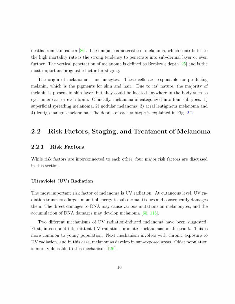
deaths from skin cancer [86]. The unique characteristic of melanoma, which contributes to

the high mortality rate is the strong tendency to penetrate into sub-dermal layer or even

further. The vertical penetration of melanoma is defined as Breslow’s depth [25] and is the

most important prognostic factor for staging.

The origin of melanoma is melanocytes. These cells are responsible for producing

melanin, which is the pigments for skin and hair. Due to its’ nature, the majority of

melanin is present in skin layer, but they could be located anywhere in the body such as

eye, inner ear, or even brain. Clinically, melanoma is categorized into four subtypes: 1)

superficial spreading melanoma, 2) nodular melanoma, 3) acral lentiginous melanoma and

4) lentigo maligna melanoma. The details of each subtype is explained in Fig. 2.2.

2.2 Risk Factors, Staging, and Treatment of Melanoma

2.2.1 Risk Factors

While risk factors are interconnected to each other, four major risk factors are discussed

in this section.

Ultraviolet (UV) Radiation

The most important risk factor of melanoma is UV radiation. At cutaneous level, UV ra-

diation transfers a large amount of energy to sub-dermal tissues and consequently damages

them. The direct damages to DNA may cause various mutations on melanocytes, and the

accumulation of DNA damages may develop melanoma [60, 115].

Two different mechanisms of UV radiation-induced melanoma have been suggested.

First, intense and intermittent UV radiation promotes melanomas on the trunk. This is

more common to young population. Next mechanism involves with chronic exposure to

UV radiation, and in this case, melanomas develop in sun-exposed areas. Older population

is more vulnerable to this mechanism [126].

10

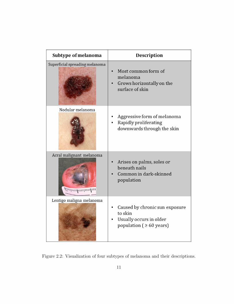
Figure 2.2: Visualization of four subtypes of melanoma and their descriptions.

11

Atypical Moles

An atypical mole is considered as a benign skin lesion, but is an unusual mole that may

resemble melanoma. A border of atypical mole is usually irregular or poorly defined. The

shape and the colour of this type of mole varies from one to another. A person with more

than five atypical moles has six times higher risk of developing melanoma compared to a

person without any atypical moles [52].

Age

Age is an important risk factor for melanoma. Melanoma occurs most commonly for those

who are aged between 40 and 60 years. The median age at diagnosis of melanoma is 57

years [110], and this is almost one decade earlier than other common cancers such as breast,

lung and colon cancers. Moreover, melanoma is one of the most common cancers in young

adults who are aged between 20 and 29 in Canada [86].

Family History

Family history of melanoma is also a risk factor. First-degree relatives of melanoma patients

have a higher risk of melanoma than those who do not have any positive family history

[56]. Familial melanoma accounts for an estimated 5− 10% of all cases of melanoma [71].

2.2.2 Staging

When the abnormal skin lesion is confirmed as malignant melanoma, the clinicians or

dermatologists determine the stage of the cancer. For melanoma, there are five stages from

stage 0 to stage IV. It is important to determine the accurate stage of melanoma because

the treatment options and prognosis is determined based on the stage of the cancer.

Stage 0 is also called melanoma in situ. At this stage, the suspected lesion is confirmed

malignant, but it is still confined to the upper layer of the skin (epidermis), and there is

12

no sign of invasion to dermal layer. The 5-year survival rate for stage 0 is greater than

99% [11].

Stage I is defined as a melanoma that grows as thick as 2mm. While the tumor pene-

trated into dermal layer, there is very low risk for the cancer to spread to lymph nodes or

distant ares. The 5-year survival rate is as high as 95% [13].

At Stage II, the thickness of melanoma is from 2mm to more than 4mm. In most cases,

the tumor is still located in dermal layer, but as it develops, it may penetrate deeper into

subcutaneous fat layer. Ulceration, which is the breakage of epidermis on the top of the

melanoma, may be observed. Stage II is considered intermediate to high risk for distant

metastasis, and the 5-year survival rate is between 45% and 79% [13].

Stage III is defined when tumor spreads into nearby lymph nodes, yet not to distant

areas. At this stage, the depth of tumor no longer matters, and the number of lymph

nodes to which the tumor has spread determines the severity of the condition. The 5-year

survival rate ranges from 24% to 67% [13].

In Stage IV, the melanoma spreads beyond the primary location to more distant areas.

The common locations of metastasis are lung, abdominal organs, or soft tissues. The

prognosis at this stage is extremely poor as the 5-year survival rate is between 9% and

28%, depending on the metastasis location [12].

2.2.3 Treatment

While treatment options highly depend on the stage of melanoma, surgery is the gold

standard of treatment [116]. Surgery could be employed for almost all stages of melanoma.

Depending on the progress of a tumor, different surgical approaches are considered. For

example, if the melanoma is still in its early stages such as Stage 0 or Stage I, simple local

excision or wide local excision may be sufficient to remove the melanoma cells. However, if

the invasion is severe and the tumor is suspected or confirmed for lymph node metastasis,

complete lymph node dissection, which removes not only skin tissue but also lymph nodes,

may be required [83]. Different treatment options other than surgery can be considered

for those who are in the late stage of melanoma, or those who cannot undergo the surgical

13

option due to size and/or location of tumor, age of patients, or comorbidity. Other options

can be 1) chemotherapy, which uses drugs to stop spreading of cancerous cells [46]; 2)

radiation therapy, which uses high energy radiation such as x-rays to kill cancerous cells or

keep them from growing [114]; and 3) immunotherapy, which boosts patients’ own immune

systems to fight against cancer [58].

2.3 Diagnosis of Melanoma

Diagnosis of melanoma typically consists of two parts: clinical examination and patho-

logical examination. Clinical examination is conducted by clinicians or dermatologists to

find any suspicious lesions by examining their appearance, while pathological examination

provides more accurate diagnosis by looking into pathology of the lesion, which is acquired

through biopsy.

2.3.1 Clinical Examination

As aforementioned, early detection of melanomic lesion is extremely important for bet-

ter outcome because the survival rate at the late stage of melanoma is dismal. In fact,

melanoma has a relatively low mortality rate compared to other major cancers. This is

because melanomic lesion can be more easily identified by clinicians or even by patient

him/herself. Initial diagnosis is usually conducted with naked eye by clinicians or derma-

tologists, and one of the most commonly used tools is the ABCDE-rule [50, 1].

ABCDE-rule serves as a guideline to distinguish malignant and benign lesion. There

are five components in ABCDE-rule, and each component is explained in Fig. 2.3

2.3.2 Imaging Techniques for Clinical Examination

For the imaging techniques during the clinical examination, the most thorough screening

at the early stage of melanoma is a total body skin examination (TBSE) [57]. The doctor

14

Figure 2.3: Clinical Examination: Explanation of ABCDE rule. Adapted from Dirk

Schadendorf et. al. [111]

15

scans the entire skin surface of the patient by visual inspection, and examines any sus-

picious moles that could be melanoma. Other than TBSE, many imaging modalities are

employed during the clinical examination for lesion-specific screening, including traditional

photography, dermoscopy, or confocal laser scanning microscopy. In this section, two of

the most common imaging modalities are discussed.

Traditional Photography

Although different imaging modalities have emerged, the traditional or dermatological

photographs still are the primary modality for melanoma. More than half of dermatol-

ogist currently employ dermatological photographs for initial examination[47, 100]. The

photographs typically show single or multiple superficial skin lesions, and these images

reproduce what a dermatologist sees with the naked eye [38]. The images are taken peri-

odically to track any changes in the lesions [14]. Typically, if no changes in colour, size or

shape have been observed, the lesion is treated as benign case. However, if changes occur

in the lesions, a biopsy of the lesion is followed for a more accurate examination.

Dermoscopy

Dermoscopy, which is also known as dermascopy, in vivo cutaneous surface microscopy or

epiluminescence microscopy, is a non-invasive imaging technique. Like traditional photog-

raphy, dermoscopy is imaging only the surface of skin. This imaging modality is equipped

with a magnifying glass that uses the cross-polarized light. Some dermoscopy has im-

mersion fluid to make the layer of skin more transparent to light and eliminate reflection

[70, 82]. The major difference between dermoscopy and traditional photography is that

dermatologists can observe lesions in detail with the magnifying glass and free from light

reflection.

At the late stage of melanoma, because metastasis likely occurs, invasive imaging tech-

niques are required. If the metastasis is thought to be local, and only around lymph nodes,

mid-frequency ultrasound is the ideal imaging method of choice because of high accuracy

[133, 10]. For distant metastasis, cross-sectional diagnostic imaging such as PET/CT, MRI

16

or CT are the standard of care [111]. While PET/CT yielded high diagnostic accuracy for

tumor localization compared to whole-body MRI or CT [133], MRI or CT are commonly

used instead, because of the high costs of PET/CT [111]. For cerebral metastases, MRI is

known to be the most precise imaging technique over PET/CT or CT [9].

2.3.3 Pathological Examination

When clinicians determines that the suspicious lesion is malignant based on the clinical

examination, the lesion is further examined in pathological examination. The first step

in pathological examination is biopsy. Biopsy is the process to take a small sample of

the lesion by excising the lesion with a lateral margin of 2-3mm, and vertically reaching

into subcutaneous fat tissue [96]. From the biopsy, pathologists produce histopathological

report on the suspicious lesion, which contains histological features for a correct diagno-

sis, staging, and the subtype of melanoma, and the final diagnosis is made based on the

report [12].

2.3.4 The Computer-aided Melanoma Diagnosis

While conventional approach of melanoma diagnosis was discussed in the previous sections,

the computer-aided melanoma diagnosis was emerged. The purpose of computer-aided

melanoma diagnosis is to aid dermatologists to have the improved accuracy on their di-

agnostic decision by providing quantitative measures on a skin lesion. The quantitative

measures can be constructed from the traditional examination scheme such as ABCD-rule,

or the skin lesion image can be analyzed using texture or shape of the lesion.

Celebi et al. designed the melanoma classification algorithm on dermoscopy images.

They generated a total of 437 features from each image based on the shape (Asymmetry,

aspect ratio, area, and compactness), colour and texture. For the classification, SVM with

radial basis function kernel was used with the feature selection. They obtained a sensitivity

of 93.3% and a specificity of 92.3% on a set of 564 images.

Dreiseitl ran a multi-class classification from pigmented skin lesion. Several classifica-

tion algorithms, including k-nearest neighbors, logistic regression, artificial neural network,

17

decision trees, and SVM are tested to classify common nevi, dysplastic nevi, or melanoma

(3 classes). The images were acquired in the form of a dermoscopy image, and 107 morpho-

metric features were extracted for each image. Among tested algorithms, logistic regression,

artificial neural network, and SVM yielded the best results.

Ruiz et al. took a slightly different approach on classification as they combined three

different classification methods (k-nearest neighbors, Bayes classification, and artificial

neural network) as a whole for making decision. A number of feature extracted was 24,

but only six features were employed for classification after the feature selection process.

This technique yielded 78.4% sensitivity and 97.8% specificity.

Cavalcanti et al. used melanin concentrations as features in their melanoma classi-

fication algorithm. To the best of our knowledge, this is the only group to implement

physiological biomarker information into the melanoma screening system. The classifica-

tion is based on two different sets of features: ABCD-rule based features, and features from

concentrations of eumelanin and pheomelanin. Then, they ran two stages of classification

in which the first stage employed k-nearest neighbor model with the ABCD-rule based fea-

tures. The second stage classification used features from melanin concentrations on Bayes

classification. To improve their results, they empirically tested a different combination of

features to find the best set of features, and ultimately obtained 99.7% of sensitivity and

96.2% of specificity.

2.4 Understanding Skin and Physiological Biomark-

ers

Although melanoma can arise in different parts of the body, it primarily originates from

skin. Therefore, to understand the structure of skin and its physiological biomarkers is a

necessary step prior to discussing physiological biomarker extraction model.

18

Figure 2.4: Illustration of the skin structure including the epidermis, the papillary dermis,and the reticular dermis. Image adapted from J. Schofield and W. Robinson [113]

2.4.1 Structure of Skin

The structure of skin can be generally divided into four different layers: the epidermis,

papillary dermis, reticular dermis and subcutaneous fat, as shown in Fig. 2.4. The epider-

mis is the outermost layer of the skin, and is mainly composed of cells called keratinocytes,

which are very strong. Although the epidermis is thin, with a thickness of 0.027-0.15 mm

[43, 73], it acts as an effective barrier to protect the body from bacteria and other mi-

croorganisms. The next layer under the epidermis is the dermis, which is much thicker,

and is responsible for providing strength and structural support to the skin. The dermis

is composed primarily of collagen, and contains blood vessels and lymphatic channels.

19

The thickness of dermal layer varies depending on the location, from 0.6-3 mm [43, 73].

For example, the dermis is very thick on the back but thin on the top of the foot. The

papillary dermis is the upper part of the dermis, and the reticular dermis is at the bottom.

The innermost skin layer is the subcutaneous fat, which maintains body heat from loss.

2.4.2 Important Physiological Biomarkers Related to Melanoma

The visible evidence of melanoma is an atypical mole, which results from the uncontrol-

lable production of melanin from melanocytes. Not only is the concentration of melanin

escalated, more blood is also required to supply oxygen and other nutrition at the lesion.

This leads to angiogenesis, which forms new blood vessels from existing ones. Angiogenesis

promotes the circulation of blood and eventually increases the concentration of hemoglobin

at the lesion. Therefore, the concentrations of melanin and hemoglobin can serve as ex-

cellent physiological biomarkers to determine whether a given lesion has the potential to

become cancerous.

Melanin

As mentioned, melanin is produced from melanocytes, which are primarily distributed

in the epidermal layer of skin. There are two main types of melanin: pheomelanin and

eumelanin. The major difference between the two melanins is the colour of pigment they

produce. While pheomelanin gives a red-yellowish colour, eumelanin colours brown-black.

Skin colour is dominated by eumelanin [125], and the ratio between the concentration

of pheomelanin and eumelanin present in human skin varies greatly from individual to

individual. The number could be as low as 0.049 for darker coloured skin and as high

as 0.36 for lighter coloured skin [92]. While a major function of melanin is providing a

protection from ultraviolet (UV) radiation, pheomelanin is known to be more vulnerable

than eumelanin to DNA damages or mutations, caused by UV radiation [31, 136]. This

vulnerability of pheomelanin suggest that pheomelanin plays an important role to develop

a cancer [32, 123].

20

There has been several studies to investigate the activities of eumelanin and pheome-

lanin in malignant melanomic lesions for the purpose of the non-invasive diagnosis. For

example, Marcheni et al. [79] conducted a retrospective analysis using diffuse reflectance

spectroscopy, and found that the level of eumelanin increases in the malignant lesions,

when compared to the benign ones. Moreover, they observed the decrease of the level of

pheomelanin in the malignant cases. This finding agrees with the study that was conducted

by Zonio et al. [141]. While the increase of the level of eumelanin is generally agreed, the

activity of pheomelanin in malignant lesion is debatable as another study concluded that

the level of pheomelanin increased in melanomic cells, when compared normal cells [108].

Zonio et al., therefore, concluded that the spectral responses are not strong enough to

obtain accurate melanin concentrations.

Hemoglobin

Hemoglobin is a type of protein and is vital to humans as it transports oxygen from respi-

ratory organs to other organs and the rest of the body. Hemoglobin is located in the red

blood cells, and the transportation of oxygen by hemoglobin is done via blood vessels. As

aforementioned, blood runs through the dermal layers in smaller vessels for the papillary

dermis and larger vessels for the reticular dermis. Normally, the hemoglobin concentration

in whole blood is between 134 and 173g/L [135], and the oxygenated hemoglobin, which is

the state with oxygen bound, can be as high as 95% in the arteries and as low as 47% in the

veins [4]. Once hemoglobin releases oxygen, it is called deoxygenated hemoglobin. Oxy-

genated and deoxygenated hemoglobin have different optical properties, and their responses

to melanoma are different as well. A study found that the concentration of oxygenated

hemoglobin is significantly lower for melanoma cases than that for benign cases, and conse-

quently, increased concentration of deoxygenated hemoglobin in melanomic cells [53]. This

phenomenon can explain hypoxia around the lesion, which is the condition of lower level

of oxygen in blood.

21

Other Features

While melanin and hemoglobin are the most important biomarkers for diagnosing melanoma,

other features such as bilirubin and β-carotene are also prevalent in blood or dermal layer,

respectively. Bilirubin is a brownish yellow pigment and provides a characteristic colour

to solid waste product. Although the limited studies are available for the relationship be-

tween the level of bilirubin in blood and melanoma, one study suggested that the increased

level of bilirubin may aggravate melanoma [17]. β-carotene is a red-orange pigment and a

pre-cursor to vitamin A, which plays important roles in vision and in maintaining normal

skin health. Like bilirubin, more thorough research needs to be conducted in order to

determine the relationship between melanoma and the given pigment, but it is believed

that β-carotene can be used to prevent cancer including skin cancer [120].

2.5 Summary

The chapter has presented background material to help understanding the remainder of

this thesis. The risk factors, staging, and treatment options of melanoma have been briefly

reviewed. Standard clinical procedures for detecting and diagnosing melanoma have been

reviewed. Furthermore, physiological biomarkers related to melanoma have been reviewed.

In the next chapter, we present a framework for extracting physiological biomarkers from

melanoma images for constructing a dermal radiomics sequence.

22

Chapter 3

Physiological Biomarker Extraction

Model

In a dermal radiomics framework, physiological biomarker extraction is the first step for

constructing a dermal radiomics sequence. In this chapter, we review the existing physio-

logical biomarker extraction methods. Moreover, we propose a novel extraction technique

for eumelanin, pheomelanin, and hemoglobin from an acquired skin lesion image using a

non-linear random forest regression model.

3.1 Light-skin Interaction Model

To extract any desired physiological biomarkers from a skin lesion image, we first need

to understand how the colour of a skin lesion in the image is produced related to the

concentrations of physiological biomarkers. The relationship between them can be found

in light-skin interaction model. When light hits the surface of skin, the incident light

undergoes various interactions within skin, and finally reflected (Fig. 3.1). The light-skin

interaction model describes the behavior of light particles based on the optical properties

of skin pigments as well as interface between skin layers.

Modeling of light interaction with skin, which is multi-layered and inhomogeneous, is

23

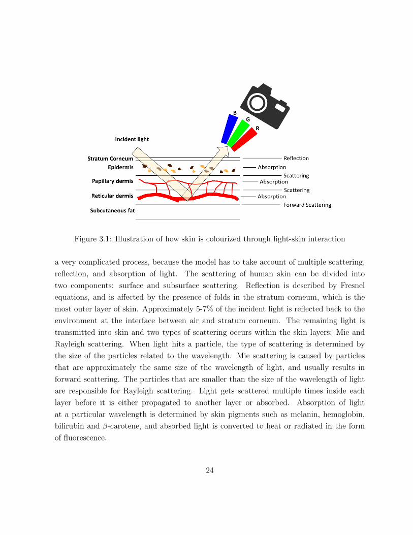
Figure 3.1: Illustration of how skin is colourized through light-skin interaction

a very complicated process, because the model has to take account of multiple scattering,

reflection, and absorption of light. The scattering of human skin can be divided into

two components: surface and subsurface scattering. Reflection is described by Fresnel

equations, and is affected by the presence of folds in the stratum corneum, which is the

most outer layer of skin. Approximately 5-7% of the incident light is reflected back to the

environment at the interface between air and stratum corneum. The remaining light is

transmitted into skin and two types of scattering occurs within the skin layers: Mie and

Rayleigh scattering. When light hits a particle, the type of scattering is determined by

the size of the particles related to the wavelength. Mie scattering is caused by particles

that are approximately the same size of the wavelength of light, and usually results in

forward scattering. The particles that are smaller than the size of the wavelength of light

are responsible for Rayleigh scattering. Light gets scattered multiple times inside each

layer before it is either propagated to another layer or absorbed. Absorption of light

at a particular wavelength is determined by skin pigments such as melanin, hemoglobin,

bilirubin and β-carotene, and absorbed light is converted to heat or radiated in the form

of fluorescence.

24

To implement these interactions under the skin, several light-skin interaction models

have been proposed based on Kubelka-Munk theory [26, 36, 43], diffusion theory [44, 48],

or Monte Carlo simulation algorithm [97, 73].

3.2 Existing Models

Extraction techniques of skin pigments are typically considered as an inverse model of

light-skin interaction model. Therefore, it is important to know how the forward model is

constructed for each extraction technique. In this section, we present several skin pigment

extraction models each with its corresponding forward model.

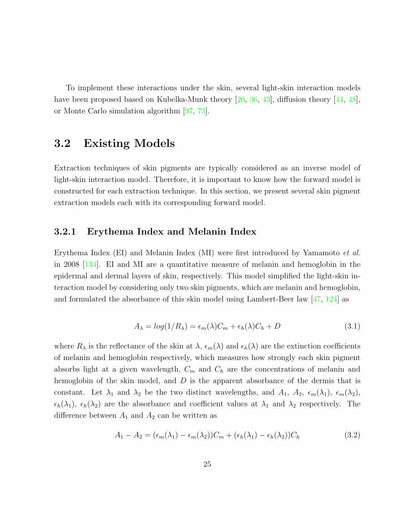
3.2.1 Erythema Index and Melanin Index

Erythema Index (EI) and Melanin Index (MI) were first introduced by Yamamoto et al.

in 2008 [134]. EI and MI are a quantitative measure of melanin and hemoglobin in the

epidermal and dermal layers of skin, respectively. This model simplified the light-skin in-

teraction model by considering only two skin pigments, which are melanin and hemoglobin,

and formulated the absorbance of this skin model using Lambert-Beer law [37, 124] as

Aλ = log(1/Rλ) = εm(λ)Cm + εh(λ)Ch +D (3.1)

where Rλ is the reflectance of the skin at λ, εm(λ) and εh(λ) are the extinction coefficients

of melanin and hemoglobin respectively, which measures how strongly each skin pigment

absorbs light at a given wavelength, Cm and Ch are the concentrations of melanin and

hemoglobin of the skin model, and D is the apparent absorbance of the dermis that is

constant. Let λ1 and λ2 be the two distinct wavelengths, and A1, A2, εm(λ1), εm(λ2),

εh(λ1), εh(λ2) are the absorbance and coefficient values at λ1 and λ2 respectively. The

difference between A1 and A2 can be written as

A1 − A2 = (εm(λ1)− εm(λ2))Cm + (εh(λ1)− εh(λ2))Ch (3.2)

25

If λ1 and λ2 are chosen so that εm(λ1)− εm(λ2) is nearly zero or significantly smaller than

εh(λ1)− εh(λ2) and A1−A2, then combining Eq. (3.1) and Eq. (3.2) make a linear function

with respect to Ch and the difference between absorbances is the erythema index. The

melanin index is computed by making εh(λ1)− εh(λ2) nearly zero. For EI, λ1 is chosen at

a wavelength of 540-570 nm, where the ‘green band’ is located and λ2 is at around 660 nm

where the ‘red band’ is located. For MI, λ1 and λ2 are set at wavelengths of 620-650 nm

and 670-700nm respectively. Therefore, the formulation of EI and MI can be expressed as

following:

EI = log(1/Rgreen)− log(1/Rred) (3.3)

MI = log(1/Rred) (3.4)

where Rgreen and Rred are the reflectance of the skin at 540 nm and 660 nm, respec-

tively. Although EI and MI hold great linearity with the concentrations of hemoglobin and

melanin, different camera settings or illumination settings may change the indices greatly.

Moreover, EI and MI do not provide the absolute concentrations of features, rather the

relative concentrations.

3.2.2 Linear Light-skin Interaction Modeling

Linear light-skin interaction modeling (LLM) was proposed by Gong and Desvignes [55].

LLM computes concentration of melanin, total hemoglobin, and oxyhemoglobin (cMel,

cHb, and cHbO2 , respectively) by first constructing linear light-skin interaction model as

following:

log(1/R(λr))

log(1/R(λg))

log(1/R(λb))

=

εHbO2(λr) εHb(λr) εMel(λr)

εHbO2(λg) εHb(λg) εMel(λg)

εHbO2(λb) εHb(λb) εMel(λb)

cHbO2

cHb

cMel

(3.5)

26

where εHbO2(λ), εHb(λ) and εMel(λ) are the tabulated extinction coefficients of oxygenated

hemoglobin, total hemoglobin and melanin [109, 140], and λr, λg, and λb are selected at

600nm, 540nm and 440nm, respectively.

As Eq. 3.5 was set up as linear equation, the concentration of melanin, total hemoglobin

and oxygenated hemoglobin can be inferred as an inverse model of Eq. 3.5 :

cHbO2

cHb

cMel

=




−1 log(1/R(λr))

log(1/R(λg))

log(1/R(λb))

(3.6)

While LLM is easy to implement and computationally efficient, the major limitation is

that the model oversimplifies the light-skin interaction. As discussed in Section 3.1, this

model only accounts for absorbance, and other light-skin interactions such as scattering

and reflectance are omitted. This model also ignores skin pigments except melanin and

hemoglobin, and does not account for all skin layers as it only considers epidermis and

dermis layers, in which melanin and hemoglobin are distributed.

3.2.3 Nearest Neighbor Model

Cavalcanti et al. [29] proposed a nearest neighbor model (NN) that extracts eumelanin

and pheomelanin concentrations from the standard camera image. To accomplish this, a

non-linear forward model was first constructed using a biophysically-based spectral model

of light-skin interaction [73], which models the way light within the visible spectrum prop-

agates in skin tissue to determine the reflectance spectra being observed by the camera.

Based on this forward model, a look-up table was constructed containing 1065 skin colours,

corresponding to various permutations of eumelanin and pheomelanin concentrations rang-

ing from 20 to 300 g/L, and from 8 to 60 g/L, with the steps of 4 g/L, respectively.

For the estimation of physiological biomarkers, an inverse model is constructed using a

nearest neighbor model. The colour of the testing sample is first matched to the colours

in the look-up table, which has the shortest squared Euclidean distance in RGB colour

27

space to the testing sample, the corresponding eumelanin and pheomelanin concentrations

is obtained for the estimation.

While NN adopts a complex forward model for physiological biomarker estimation, NN

has a couple of limitations on performing this task. First, the possible estimation is limited

to 71 values, and 14 values for the eumelanin and pheomelanin, respectively. Second, due

to the nature of nearest neighbor model, the algorithm has to perform an exhaustive search

on a look-up table for each estimation, which may increase computational complexity.

3.3 Proposed Random Forest Model

In this section, a novel non-linear random forest regression model for extracting physio-

logical biomarkers from dermatological images is described. The proposed computational

model is designed to overcome the limitations of existing models in the literature, by

enabling the modeling of complex, non-linear light-skin interactions (MI/EI and LLM)

while maintaining greater flexibility and reduced computational complexity (NN). First,

the proposed non-linear light-skin interaction model is constructed as the forward model

(Section 3.3.1). Second, the proposed random forest inverse light-skin interaction model

and how it is learned is then described in detail (Section 3.3.2).

3.3.1 Non-linear, Forward Light-skin Interaction Model

As described by the LLM and NN models, the physiological biomarker extraction technique

can be considered as solving an inverse problem of light-skin interaction model. Therefore, a

non-linear light-skin interaction is first proposed as a forward model with input parameters

as concentrations of eumelanin, pheomelanin, and hemoglobin, and outputs as intensity

values in different colour spaces, including RGB. The proposed forward model is composed

of two parts. The first part is the computational light-skin interaction model, which was

proposed by Baranoski and Krishnaswamy [15, 72], and the second part is a tristimulus

value calculation, which generates 14 intensity values from five different colour spaces. The

visual illustration of the proposed forward model is shown in Fig. 3.2.

28

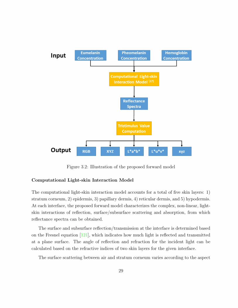
Figure 3.2: Illustration of the proposed forward model

Computational Light-skin Interaction Model

The computational light-skin interaction model accounts for a total of five skin layers: 1)

stratum corneum, 2) epidermis, 3) papillary dermis, 4) reticular dermis, and 5) hypodermis.

At each interface, the proposed forward model characterizes the complex, non-linear, light-

skin interactions of reflection, surface/subsurface scattering and absorption, from which

reflectance spectra can be obtained.

The surface and subsurface reflection/transmission at the interface is determined based

on the Fresnel equation [121], which indicates how much light is reflected and transmitted

at a plane surface. The angle of reflection and refraction for the incident light can be

calculated based on the refractive indices of two skin layers for the given interface.

The surface scattering between air and stratum corneum varies according to the aspect

29

ratio of the stratum corneum folds, which is represented as ellipsoids in this model. The

aspect ratio (σ ∈ [0, 1]) of the stratum corneum folds is defined as the quotient of the

length of the vertical axis by the length of the horizontal axis, which are parallel and

perpendicular to the specimen’s normal respectively. As the folds become flatter (lower σ),

the reflected light becomes less diffuse. To account for this effect, the model employed a

surface-structure function, which represents rough air-material interfaces using microareas

randomly curved [127]. The scattering is determined in terms of the polar angle given by :

α = arccos

[((

σ2

√σ4 − σ4s+ s

− 1)1

σ2 − 1)1/2]

(3.7)

where s is the irregularity of surface of stratum corneum. For a ray that enters the epi-

dermis, the scattering is determined using azimuthal (β) and the polar angles where β is

ranged between 0 and 2π, and the polar scattering angles measured by [26]. Every ray en-

tering dermis layer is tested for Rayleigh scattering. For the testing, the spectral Rayleigh

scattering amount, S(λ), is calculated as following:

S(λ) =8tπ3((

ηfηm

)2 − 1)2

0.63cosθ(43r3π)−1λ4

(3.8)

where ηf is index of refraction of the fibers, ηm is index of refraction of the dermal medium,

t is the thickness of the medium, θ is the angle between the ray direction and the specimen’s

normal direction, and r is radius of collagen fibrils. The ray is scattered with a probability

of 1− exp−S(λ).

Once a ray has been scattered, it is tested for absorption. The absorption testing is

performed every time a ray enters into a new layer. For the testing, the ray free path

length based on Beer’s law [129] was calculated as following:

p(λ) = −Acosθµai(λ)

(3.9)

where A is the absorbance of a given layer, θ is the angle between the ray and the spec-

imen’s normal, and µai(λ) is the total absorption coefficient of a given layer, i. Total

absorption coefficient for each layer is obtained by multiplying the spectral extinction coef-

ficient of the pigment by its estimated concentration in the layer. Eumelanin, pheomelanin,

30

oxyhemoglobin, deoxyhemoglobin, bilirubin and β-carotene are taken into account in this

model. If p(λ) is greater than the thickness of the given layer, then the ray is propagated,

otherwise it is absorbed.

Tristimulus Value Computation

From this computational light-skin interaction model, the reflectance spectra, R(λ), is

collected, and is further processed to calculate outputs of the forward model, which are

the intensity values from 14 individual channels of RGB, XYZ, L*a*b*, L*u*v*, and xyz

colour space.

While the RGB spectral bands are used to define colour in a standard camera image,

the mapping from the reflectance values to RGB colour space involves an intermediate

step, which is the colour tristimulus values, XYZ. XYZ colour space was first introduced

by the International Commission on Illumination (CIE) in 1931 to describe the colour

space mathematically. This colour space was derived from the RGB model and expanded

beyond the RGB colour space. The XYZ can be calculated by the additive law of colour

matching [77].

X = N∑λ

R(λ)S(λ)x(λ)∆λ, (3.10)

Y = N∑λ

R(λ)S(λ)y(λ)∆λ, (3.11)

Z = N∑λ

R(λ)S(λ)z(λ)∆λ, (3.12)

where S(λ) is the relative spectral power distribution of the illuminant; R(λ) is the

reflectance function, which were modeled from the computational light-skin interaction

model; x(λ), y(λ) and z(λ) are the spectral sensitivity functions, and ∆λ is the wavelength

interval. For our experiment, CIE standard Illuminant D65 was used for S(λ), and the

CIE 1931 sensitivity functions of the standard observer for 2◦ and ∆λ = 5nm were em-

ployed for the spectral sensitivity function, x(λ), y(λ) and z(λ), and wavelength intervals,

respectively. The constant N was defined as

31

N =∑λ

S(λ)y(λ)∆λ (3.13)

Once tristimulus values XYZ are obtained, they are converted to the RGB, L*a*b*,

L*u*v*, and xyz colour spaces. While the colour is conventionally defined in RGB colour

space, the forward model extends into a total of five colour spaces to define each colour,

which is created based on light-skin interaction model. The main reason for this extension

is that using three colour channels from RGB may not be sufficient to generate an accurate

inverse model. As each color space has an unique representation of the color, generating

14 colour channels in forward model eventually leads to more robust construction of its

inverse model. The detail of colour conversion from XYZ to other colour spaces can be

found in Appendix A.

3.3.2 Non-linear Random Forest Inverse Light-skin Interaction

Model

In the previous section, we presented a non-linear forward model, which uses concentration

of physiological biomarkers to generate intensities of 14 different colour channels as shown

in Fig. 3.2. This forward model uses non-linear light-skin interactions. To construct the

associated inverse model, which predicts the concentration of physiological biomarkers from

14 colour channels, random forest regression is employed.

Random forest is an ensemble learning technique for classification and regression that

works by constructing a large number of decision trees [24]. This technique was introduced

by Breiman[24], and is widely used in machine learning problems. Important components

of random forest are the bagging technique and the construction of a decision tree. In the

next section, decision tree learning and bagging technique are explained to understand the

random forest model.

32

Decision Tree Learning

A decision tree is a machine learning technique to predict a label in class variable from

predictor variables using a binary tree. Given that Xi for i = 1, 2, ...k, is a set of predictor

variables, and Y is its corresponding class variable, decision tree is growing as following:

1. Start at the root node

2. At each node, find a subset of X based on an attribute value test (i.e., minimizing

the sum of Gini indexes). Use the subset to split the node into two child nodes.

3. Repeat step 2 for each child node until the splitting does not add any values to the

prediction, or the predetermined threshold is reached.

In a decision tree, each internal node, which has its’ child nodes, is typically labeled

with a single predictor variable, and each leaf, which does not have child nodes, is labeled

with a class.

Bagging

Bagging or bootstrap aggregating is a classification method, which uses multiple learning

classifiers (i.e., decision tree) for prediction. This technique is designed to improve the

stability and accuracy by avoiding overfitting, which is the common problem in decision

trees.

Given a training set of Si for i = 1, 2, ..., n, the bagging algorithm trains the classifiers

as following:

1. Generate a net set, S ′, by randomly sampling n samples with replacement from the

original training set, S.

2. Train a classifier (i.e., decision tree) based on the new set, S ′.

3. Repeat Step 1-2 t times

33

After the training stage, bagging produces t number of classifiers. For each test example,

t classifiers are fitted and the results of all t trees are averaged for a final prediction value

for regression.

From bagging to random forest

While random forest and bagging generates many decision trees to aggregate the result,

the main difference between bagging and random forest is how each decision tree grows.

In bagging, all of predictor variables are considered for splitting at each interior node. In

random forest, only a subset of predictor variables are responsible for splitting at each node,

and the subsets are chosen randomly from the predictor variables. The default value for

the number of a subset at each node, mtry, is√k for classification and k/3 for regression,

where k is a total number of predictor variables. Therefore, bagging can be viewed as

a special case of random forest with mtry = k. The main reason of bringing additional

randomization into the random forest algorithm is to reduce variance to improve accuracy.

Since random forest is constructed based on decision trees, it is always exposed to a problem

of high variance. Because random forest introduces randomness for growing a decision tree

as well as sampling the training set, it can effectively offset the problem of high variance

without sacrificing low bias.

Training of the proposed random forest inverse model

For our inverse model, the concentration of eumelanin, pheomelanin, and hemoglobin is

predicted by individual random forest regression model. To train each model, the training

data is constructed using the proposed non-linear light-skin interaction forward model. The

input variables, which are the concentration of eumelanin, pheomelanin, and hemoglobin,

are varied from 50 g/L to 350 g/L for eumelanin, from 8 g/L to 92 g/L for pheomelanin,

and from 120 g/L to 188 g/L for hemoglobin, with the steps of 4 g/L. Other parameters for

the forward model are set to default values. The proposed non-linear light-skin interaction

forward model then generates the reflectance spectra via Monte-Carlo light propagation

simulation [72], where the light propagation is simulated as a random walk process using ray

34

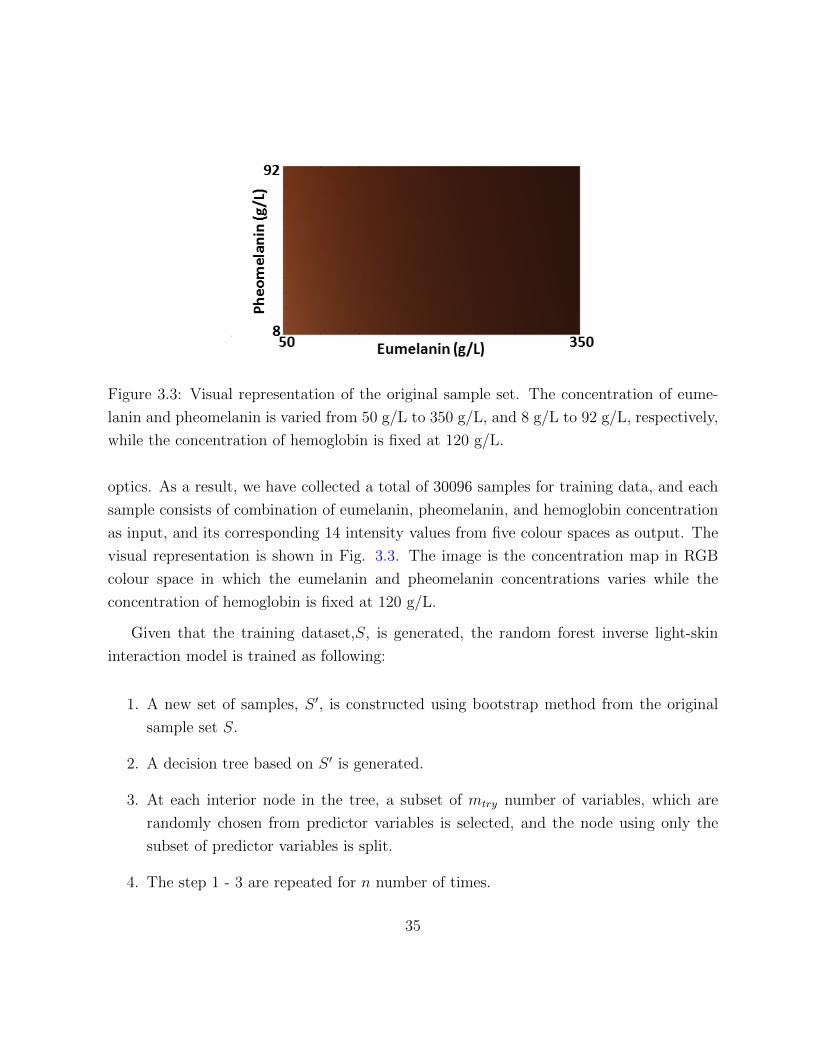
Figure 3.3: Visual representation of the original sample set. The concentration of eume-

lanin and pheomelanin is varied from 50 g/L to 350 g/L, and 8 g/L to 92 g/L, respectively,

while the concentration of hemoglobin is fixed at 120 g/L.

optics. As a result, we have collected a total of 30096 samples for training data, and each

sample consists of combination of eumelanin, pheomelanin, and hemoglobin concentration

as input, and its corresponding 14 intensity values from five colour spaces as output. The

visual representation is shown in Fig. 3.3. The image is the concentration map in RGB

colour space in which the eumelanin and pheomelanin concentrations varies while the

concentration of hemoglobin is fixed at 120 g/L.

Given that the training dataset,S, is generated, the random forest inverse light-skin

interaction model is trained as following:

1. A new set of samples, S ′, is constructed using bootstrap method from the original

sample set S.

2. A decision tree based on S ′ is generated.

3. At each interior node in the tree, a subset of mtry number of variables, which are

randomly chosen from predictor variables is selected, and the node using only the

subset of predictor variables is split.

4. The step 1 - 3 are repeated for n number of times.

35

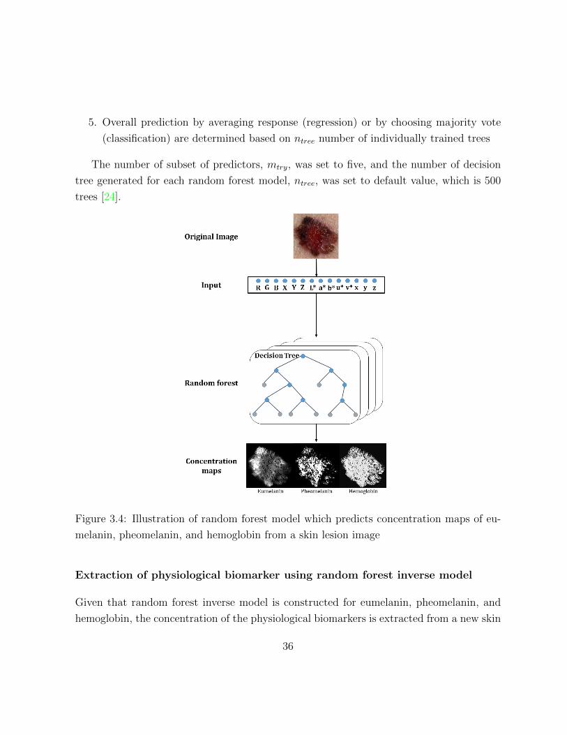
5. Overall prediction by averaging response (regression) or by choosing majority vote

(classification) are determined based on ntree number of individually trained trees

The number of subset of predictors, mtry, was set to five, and the number of decision

tree generated for each random forest model, ntree, was set to default value, which is 500

trees [24].

Figure 3.4: Illustration of random forest model which predicts concentration maps of eu-

melanin, pheomelanin, and hemoglobin from a skin lesion image

Extraction of physiological biomarker using random forest inverse model

Given that random forest inverse model is constructed for eumelanin, pheomelanin, and

hemoglobin, the concentration of the physiological biomarkers is extracted from a new skin

36

lesion image as following:

1. From a skin lesion image, each pixel is treated as an individual sample, and RGB

intensity values at each sample are processed to generate 14 predictor variables based

on the conversion equation in Appendix A.

2. The random forest inverse model of eumelanin, pheomelanin, and hemoglobin is

employed to each sample.

3. For each sample, the concentration of eumelanin, pheomelanin, and hemoglobin is

predicted.

The visual representation of extraction of physiological biomarker is shown in Fig. 3.4.

3.4 Summary

In this chapter, we discussed light-skin interaction model, which is treated as a forward

model to extract physiological biomakrers. To develop physiological biomarker extraction

model, we implemented computational light-skin interaction model and extended it so

the forward model takes the concentration of eumelanin, pheomelanin, and hemoglobin

as input variables, and computes 14 intensity values from five different colour spaces as

outputs. Then, the novel physiological biomarker extraction technique was proposed as an

inverse model of light-skin interaction model. In the next chapter, the experimental design

and the results are reported for the proposed physiological extraction technique.

37

Chapter 4

Experimental Results For

Physiological Biomarker Extraction

In the previous chapter, the novel physiological feature extraction technique for eumelanin,

pheomelanin, and hemoglobin was presented. This chapter presents a series of validation

experiments to examine how the proposed method performs compared to existing tech-

niques.

4.1 Testing Algorithms

In this validation study, five existing methods, including MI/EI, LLM, NN, AdaBoost

and bagging, are employed to compare with the proposed random forest regression model

for physiological biomarker extraction. The first three methods (MI/EI, LLM, and NN)

were described in Section 3.2, and two additional techniques are included for compari-

son. Although bagging and AdaBoost have not been adapted into physiological biomarker

extraction to the best to our knowledge, both are categorized as the ensemble learning

technique in which the proposed random forest model is. Therefore, AdaBoost and bag-

ging will provide a good comparison how the proposed method performs compared to its

similar algorithms. Moreover, the LLM can not distinguish eumelanin and hemoglobin,

38

and NN by design extracts eumelanin and pheomelanin only. Therefore, we made some

modifications on LMM and NN for better comparison.

4.1.1 Linear Light-skin Interaction Modeling

In the original algorithm in Section 3.2.2, the mixing matrix, A, is constructed as follow

to extract eumelanin, hemoglobin, and oxygenated hemoglobin.

A =




(4.1)

However, in our validation, we do not employ the oxygenated hemoglobin as a biomarker,

but pheomelanin. Therefore, we updated the mixing matrix by replacing hemoglobin with

pheomelanin and the light-skin interaction forward model (Eq. 3.5) is modified as following:

−log(r)

−log(g)

−log(b)

=

εEuMel(λr) εPhMel(λr) εHb(λr)

εEuMel(λg) εPhMel(λg) εHb(λg)

εEuMel(λb) εPhMel(λb) εHb(λb)

cEuMel

cPhMel

cHb

(4.2)

where εPhMel(λ) is the extinction coefficients of pheomelanin, which is obtained from the

study conducted by Sarna and Sealy [109].

4.1.2 Cavalcanti’s Nearest Neighbor Model

The look-up table, used by the original NN algorithm [29], contains 1065 skin colours

that are obtained from their forward model based on the permutation of 71 eumelanin

values and 15 pheomelanin values. This look-up table, however, is missing the hemoglobin

component. Here, the look-up table is made more comprehensive by augmenting it with the

hemoglobin component using the light-skin interaction model described in Section 3.3.2.

The improved look-up table contains a total of 30096 skin colours, that corresponds to

various permutation of the concentrations of eumelanin, pheomelanin, and hemoglobin.

39

4.1.3 Ensemble Techniques

As the proposed random forest inverse model is an ensemble learning technique, we im-

plemented two other ensemble regression models, which are bagging and AdaBoost, for

comparison.

Bagging

Bagging(BA) is similar to random forest model in a way that both generate a large number

of decision trees to draw a result. However, for growing a decision tree, all predictor

variables are considered for splitting at each interior node in bagging. In random forest,

only a subset of predictor variables is responsible for splitting at each node, and the subset

are chosen randomly from the predictor variables. As a result, bagging can be viewed as a

special case of random forest to use all predictor variables for splitting instead of a subset

of predictor.

AdaBoost

AdaBoost(AB) is an ensemble learning technique that uses multiple classifiers to aggregate

a result. However, while random forest trains a classifier based on a training set, which is

generated by bootstrapping, each classifier in AdaBoost is trained on a training set, which

is weighted based on the performance of the previous classifier. The weight is increased on

the training sample, which was misclassified by the previous classifier, and decreased with

correctly classified. At each iteration, AdaBoost picks one classifier with the lowest cost

(error).

In this study, AdaBoost is adapted from a commercial software package (MATLAB2011a,

The MathWorks Inc., Natick, MA), and the same training set, which was used for the pro-

posed method are employed for both bagging and AdaBoost methods.

40

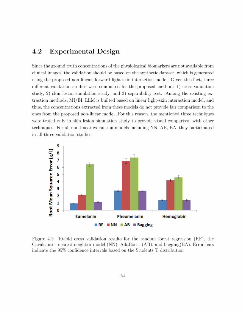
4.2 Experimental Design

Since the ground truth concentrations of the physiological biomarkers are not available from

clinical images, the validation should be based on the synthetic dataset, which is generated

using the proposed non-linear, forward light-skin interaction model. Given this fact, three

different validation studies were conducted for the proposed method: 1) cross-validation

study, 2) skin lesion simulation study, and 3) separability test. Among the existing ex-

traction methods, MI/EI, LLM is builted based on linear light-skin interaction model, and

thus, the concentrations extracted from these models do not provide fair comparison to the

ones from the proposed non-linear model. For this reason, the mentioned three techniques

were tested only in skin lesion simulation study to provide visual comparison with other

techniques. For all non-linear extraction models including NN, AB, BA, they participated

in all three validation studies.

Figure 4.1: 10-fold cross validation results for the random forest regression (RF), theCavalcanti’s nearest neighbor model (NN), AdaBoost (AB), and bagging(BA). Error barsindicate the 95% confidence intervals based on the Students T distribution

41

4.2.1 Cross Validation

From the non-linear, forward light-skin interaction model using different permutations of

physiological features, a total of 30096 samples were collected. The training data were

randomly selected from 90% of the samples, and the accuracies were calculated from the

remaining 10% of testing data. The random selection and testing was repeated 10 times,

and the average root mean squared error (RMSE) was computed as a measure of accuracy.

The results from the cross validation are presented in Fig. 4.1.

4.2.2 Skin Lesion Simulation Study

To investigate the proposed algorithm in a more clinical setting, a simulation study, which

is based on clinical skin lesion images, was conducted. A chief limitation of using a clinical

skin lesion image in validation is that there is no known method to acquire the ground truth

concentrations of physiological features. To overcome this issue, a simulated image was

constructed based on a clinical image. While the extract concentration of the skin lesion

cannot be found, the simple ensemble technique (e.g. bagging) was employed to obtain the

estimated concentration map of physiological biomarkers for the simulated image. This

step ensures that the simulated image contains a realistic concentration map of eumelanin,

pheomelanin, and hemoglobin, which can be served as ground truth. To construct these

images, a clinical image of a malignant lesion was chosen and delineated. To assign the

concentrations of physiological features at each pixel, the following steps were taken.

1. A simple ensemble technique, trained only using RGB intensities as predictors, was

employed to estimate the initial concentrations for each physiological feature.

2. For each estimated concentration, randomly generated noise that ranges from −2 to

2 g\L was added.

3. Final concentrations of each physiological feature were recorded as ground truth.

A total of ten simulated images, consisting of seven malignant and three benign images,

were constructed and tested on RF, NN, AB and BA as well as MF and MI/EI. Similar to

42

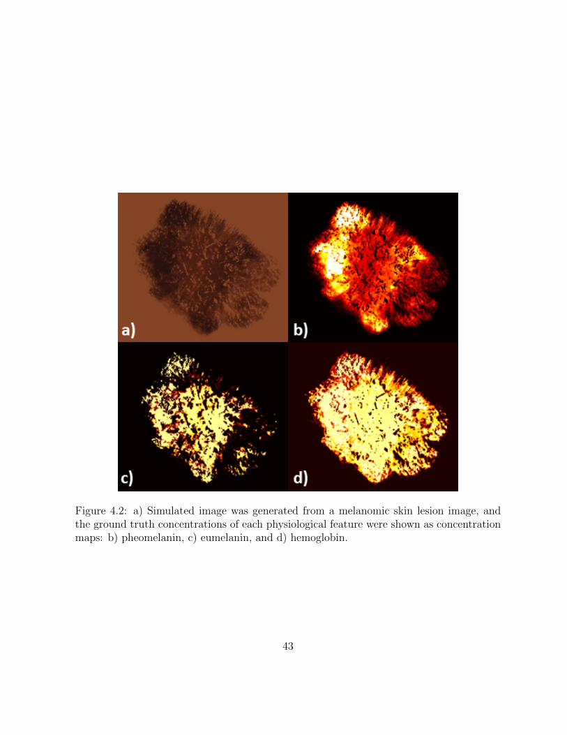
Figure 4.2: a) Simulated image was generated from a melanomic skin lesion image, andthe ground truth concentrations of each physiological feature were shown as concentrationmaps: b) pheomelanin, c) eumelanin, and d) hemoglobin.

43

Figure 4.3: RMSE from the predicted concentrations by RF, NN, AB and BA. Error barsindicate the 95% confidence intervals based on the Students T distribution

the cross validation study, RMSE was computed for each case. The results are shown in

Fig. 4.3, and visual representation of eumelanin, pheomelanin, and hemoglobin are shown

in Figs. 4.4, 4.5, and 4.6, respectively.

4.2.3 Clinical Validation

For clinical validation, the separability test was conducted. The rationale behind conduct-

ing a separability test is that the physiological features are extracted to ultimately classify

malignant lesions against benign ones. The separability test measures the strength of each

feature to discriminate between the two classes (benign and malignant melanoma). Among

different classification algorithms, Fisher’s linear discriminant analysis (FDA) was chosen

[119]. The mathematical formulation of FDA is:

J(w) =|m1 −m2|2

s21 + s22(4.3)

44

Figure 4.4: a) Ground truth concentration of eumelanin in a simulated image was predictedby b) RF, c) NN, d) AB, e) BA, f) MI/EI, and g) MF.

Figure 4.5: a) Ground truth concentration of pheomelanin in a simulated image was pre-dicted by b) RF, c) NN, d) AB, e) BA, and f) MF.

45

Figure 4.6: a) Ground truth concentration of hemoglobin in a simulated image was pre-dicted by b) RF, c) NN, d) AB, e) BA, f) MI/EI, and g) MF.

46

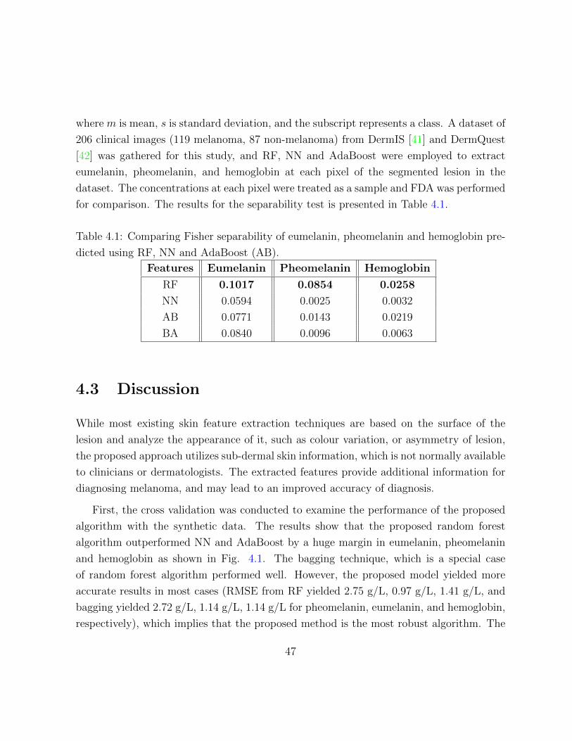
where m is mean, s is standard deviation, and the subscript represents a class. A dataset of

206 clinical images (119 melanoma, 87 non-melanoma) from DermIS [41] and DermQuest

[42] was gathered for this study, and RF, NN and AdaBoost were employed to extract

eumelanin, pheomelanin, and hemoglobin at each pixel of the segmented lesion in the

dataset. The concentrations at each pixel were treated as a sample and FDA was performed

for comparison. The results for the separability test is presented in Table 4.1.

Table 4.1: Comparing Fisher separability of eumelanin, pheomelanin and hemoglobin pre-

dicted using RF, NN and AdaBoost (AB).

Features Eumelanin Pheomelanin Hemoglobin

RF 0.1017 0.0854 0.0258

NN 0.0594 0.0025 0.0032

AB 0.0771 0.0143 0.0219

BA 0.0840 0.0096 0.0063

4.3 Discussion

While most existing skin feature extraction techniques are based on the surface of the

lesion and analyze the appearance of it, such as colour variation, or asymmetry of lesion,

the proposed approach utilizes sub-dermal skin information, which is not normally available

to clinicians or dermatologists. The extracted features provide additional information for

diagnosing melanoma, and may lead to an improved accuracy of diagnosis.

First, the cross validation was conducted to examine the performance of the proposed

algorithm with the synthetic data. The results show that the proposed random forest

algorithm outperformed NN and AdaBoost by a huge margin in eumelanin, pheomelanin

and hemoglobin as shown in Fig. 4.1. The bagging technique, which is a special case

of random forest algorithm performed well. However, the proposed model yielded more

accurate results in most cases (RMSE from RF yielded 2.75 g/L, 0.97 g/L, 1.41 g/L, and

bagging yielded 2.72 g/L, 1.14 g/L, 1.14 g/L for pheomelanin, eumelanin, and hemoglobin,

respectively), which implies that the proposed method is the most robust algorithm. The

47

statistical significant testing was performed between testing algorithms and showed that

the results obtained from the proposed method are statistically significant as shown in

Table 4.2.

Table 4.2: Two-sample t-test between the proposed physiological biomarker extraction

technique and the existing extraction methods

p-value Eumelanin Pheomelanin Hemoglobin

NN <0.001 <0.001 <0.001

AB <0.001 <0.001 <0.001

Bagging <0.001 0.185 0.019

Second, the skin lesion simulation study was conducted. A simulated image was created

to mimic actual skin lesions with known concentrations of physiological biomarkers. A total

of ten simulated images were generated and tested. In the results, the proposed method

showed the superior performance over other methods in all of physiological biomarkers.

The simulated images consists of seven malignant and three benign images. Since the skin

lesion simulation study is the closest to the clinical setting with the ground truth, we can

infer that the proposed method can perform well not only malignant cases but also benign

cases.

Last, the separability test and malignant melanoma classification were performed as

clinical validation. The separability test is designed to examine the accuracy and the

robustness of each testing algorithm when performing on clinical lesions. To bypass the

problem that the exact concentrations of each biomarkers on skin lesion is not available

in clinical image dataset, a linear separability test (i.e., Fisher’s linear discriminant) was

employed. The corresponding concentration on every pixel of lesion was treated as a sam-

ple, and all of the samples were aggregated and underwent Fisher’s linear discriminant for

each biomarker. The Fisher separability shows the ability of each biomarker to differen-

tiate benign and malignant lesion. As shown in Table 4.1, the biomarkers extracted from

the proposed method outperform over the ones from NN and AB. Although these results

do not provide direct comparison on the feature extraction accuracy, the results certainly

infer the performance of each algorithm when dealing with actual clinical lesions, which

the proposed method is preferable.

48

4.4 Summary

In this chapter, we conducted several validation studies to examine the performance of

proposed non-linear random forest inverse light-skin interaction model. A total of five

existing methods (MI/EI, LMM, NN, AB, and BA) were employed for the validation. and

the proposed method showed the superior accuracy on predicting physiological biomarkers.

In the next chapter, we construct the dermal radiomics sequence based on the extracted

physiological biomarker information.

49

Chapter 5

Dermal Radiomics Sequence

5.1 Introduction

As aforementioned in Chapter 1, radiomics is a new cancer diagnostic tool that centers

around the high throughput extraction of quantitative features from medical images to

quantify tumor phenotypes. A radiomics sequence is a set of quantitative features, which

are extracted using different data-characterization algorithms. In dermal radiomics, the

original skin lesion images as well as their corresponding concentration maps, which are

generated by the proposed method in Chapter 3, are utilized for feature extraction. As a

result, a dermal radiomics sequence consists of four different sub-feature sets as illustrated

in Fig. 5.1: i) low-level feature set (LLF), ii) high-level intuitive feature set (HLIF), iii)

physiological feature set (PF), and iv) physiological texture feature set (PTF). While the

first two sets are adapted from the existing techniques [28, 3], the last two are novel feature

sets, which are based on the physiological biomarkers of the skin lesion. In the following

section, construction of each feature set is explained.

50

Figure 5.1: Detailed block diagram of the proposed dermal radiomics sequence.

5.2 Existing Dermal Radiomics Feature Set

5.2.1 Low Level Feature

Low level feature set (LLF) consists of a total of 52 features that are extracted based on

ABCD-rule. This set is originally proposed by Cavalcanti and Scharcanski [28], and it

quantifies ABCD-rule with simple mathematical formulations. LLF is adapted into dermal

radiomics sequence because it provides a thorough characterization of a skin lesion based

on asymmetry, border irregularity, colour variation and structural difference. The full list

of 52 features is shown below.

1. Features that describe the asymmetry of lesion.

• f1: The ratio between the lesion area and its convex hull area (solidity).

• f2: The ratio between the lesion area and its bounding box area (extent).

51

• f3: Equivalent diameter.

• f4: Circularity.

• f5: The ratio between the principle axes.

• f6: The ratio between sides of a bounding box containing the lesion.

• f7: The ratio between the lesion perimeter and its area.

• f8: The difference between the areas in the lesion that are divided by the major

axis divided by the lesion area.

• f9: The difference between the areas in the lesion that are divided by the minor

axis divided by the lesion area.

• f10: The ratio of the areas divided by the major axis.

• f11: The ratio of the areas divided by the minor axis.

2. Features that describe the border irregularity of lesion

• f12−14: The average gradient magnitude of the pixels in the dilated lesion rim,

in each one of the three colour channels.

• f15−17: The variance of the gradient magnitude of the pixels in the dilated lesion

rim, in each one of the three colour channels.

• f18−20: Dividing the lesion into 8 symmetric regions and computing the average

gradient magnitudes across the dilated rim, in each of the three colour channels.

• f21−23: Dividing the lesion into 8 symmetric regions and computing the variance

of the gradient magnitudes across the dilated rim, in each of the three colour

channels.

3. Features that describe the colour variation of lesion

• f24−27: Maximum, minimum, mean and variance of the pixels intensities inside

the lesion segment in the colour variation channel.

• f28−39: Maximum, minimum, mean and variance of the pixels intensities inside

the lesion segment in each of the colour channels.

52

• f40−42: Ratios between mean values of the three original colour channels.

• f43−48: A count of the pixels who match the six hues typically associated with

melanoma.

4. Features that describe the differential structure of lesion

• f49−52: The maximum, minimum, mean and variance of the pixels intensities

inside the lesion segment to represent the textural variation.

5.2.2 High-level Intuitive Feature

High-level intuitive feature set (HLIF) is a mathematical model to describe the ABCD-

rule with human-observable characteristics, which can be intuited in natural way [3]. HLIF

consists of ten features which are derived based on the asymmetry, the border irregularity

and the colour variation of lesion, like LLF. The main difference between LLF and HLIF

is, however, that the scores from HLIF can be interpreted by dermatologists or clinicians,

while LLF does not provide any clinically relevant information by themselves. Although

clinical relevance from each feature to melanoma is not absolutely necessary in radiomics

sequence, HLIF adds variety on lesion characterization along with LLF.

Details of HLIF is described below:

1. Features that describe the asymmetry of lesion.

• f1: Colour asymmetry score.

• f2: Structural asymmetry score.

2. Features that describe the border irregularity of lesion

• f3: Fine irregularity score.

• f4: Coarse irregularity score.

3. Features that describe the colour variation of lesion

53

• f5: Reconstruction error between one-vs-two colour patches

• f6: Reconstruction error between one-vs-five colour patches

• f7: Mean difference between one-vs-five colour patches

• f8: Mean difference between two-vs-five colour patches

• f9: Colour signature difference between one-vs-two colour patches

• f10: Colour signature difference between two-vs-five colour patches

5.3 Proposed Dermal Radiomics Feature Set

In this section, two feature sets are proposed: physiological feature set and physiological

texture set. The main similarity between these two sets is that the construction is based

on the concentration maps of physiological biomarkers. While PF uses the concentration

map from RGB colour space, PTF utilizes up to five colour spaces. Each set is explained

below.

5.3.1 Physiological Feature

A physiological feature set (PF) characterizes how concentration of physiological biomark-

ers is related to melanoma. PF is composed of nine features, and each feature in PF

captures relevant information between physiological biomarkers and melanoma, which can

be conveyed to dermatologists in an intuitive manner. First six features describe the mean

and the variance of the different physiological biomarkers. As explained in Section 2.4.2,

it is known that the overall concentration level is increased for eumelanin and hemoglobin

if the lesion is malignant. Moreover, the variance of concentration in the lesion is expected

to increase because the cancer cell is not growing uniformly, resulting in colour and border

of lesion irregularity.

Last three features measures spatial heterogeneity. Spatial heterogeneity of physiologi-

cal biomarkers is the extension of colour variation in ABCD-rule. As the ABCD-rule states,

colour variation within the lesion is the important characteristic for diagnosing malignant

54

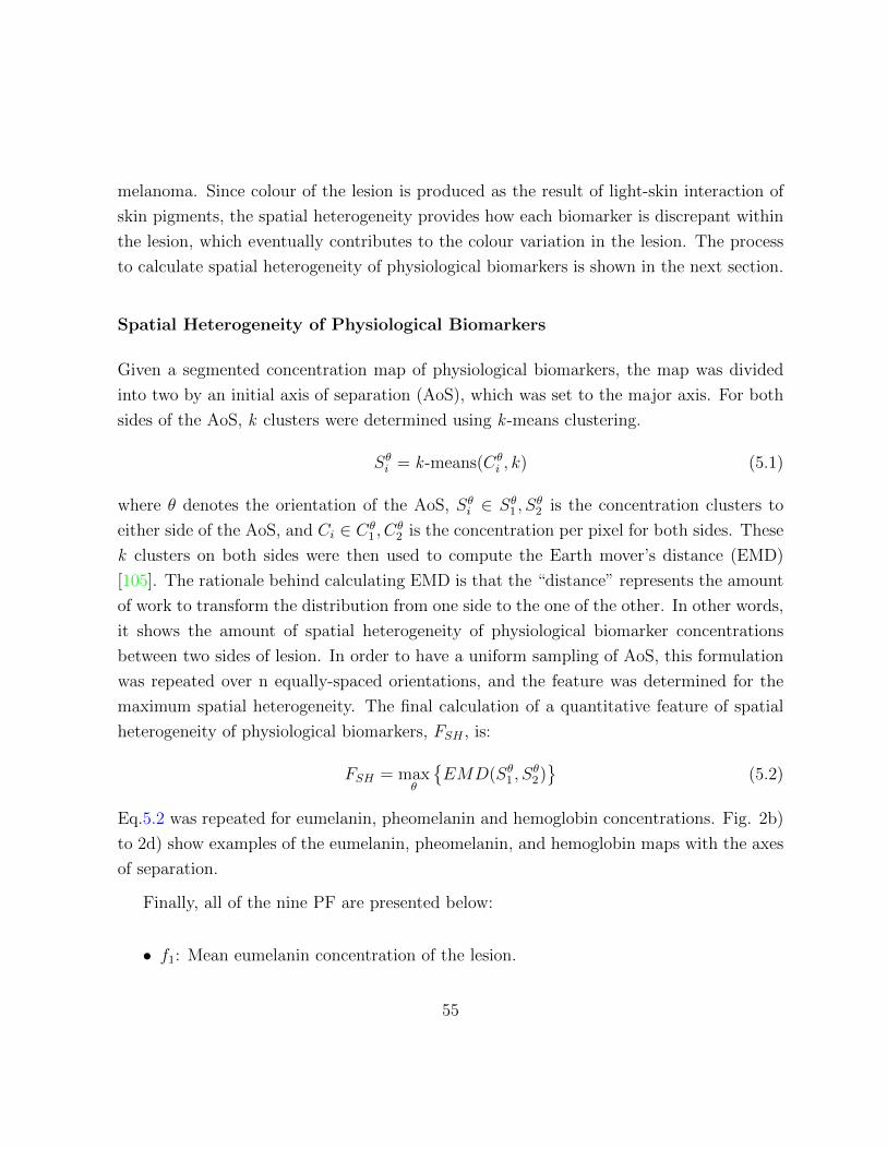
melanoma. Since colour of the lesion is produced as the result of light-skin interaction of

skin pigments, the spatial heterogeneity provides how each biomarker is discrepant within

the lesion, which eventually contributes to the colour variation in the lesion. The process

to calculate spatial heterogeneity of physiological biomarkers is shown in the next section.

Spatial Heterogeneity of Physiological Biomarkers

Given a segmented concentration map of physiological biomarkers, the map was divided

into two by an initial axis of separation (AoS), which was set to the major axis. For both

sides of the AoS, k clusters were determined using k -means clustering.

Sθi = k -means(Cθi , k) (5.1)

where θ denotes the orientation of the AoS, Sθi ∈ Sθ1 , Sθ2 is the concentration clusters to

either side of the AoS, and Ci ∈ Cθ1 , C

θ2 is the concentration per pixel for both sides. These

k clusters on both sides were then used to compute the Earth mover’s distance (EMD)

[105]. The rationale behind calculating EMD is that the “distance” represents the amount

of work to transform the distribution from one side to the one of the other. In other words,

it shows the amount of spatial heterogeneity of physiological biomarker concentrations

between two sides of lesion. In order to have a uniform sampling of AoS, this formulation

was repeated over n equally-spaced orientations, and the feature was determined for the

maximum spatial heterogeneity. The final calculation of a quantitative feature of spatial

heterogeneity of physiological biomarkers, FSH , is:

FSH = maxθ

{EMD(Sθ1 , S

θ2)}

(5.2)

Eq.5.2 was repeated for eumelanin, pheomelanin and hemoglobin concentrations. Fig. 2b)

to 2d) show examples of the eumelanin, pheomelanin, and hemoglobin maps with the axes

of separation.

Finally, all of the nine PF are presented below:

• f1: Mean eumelanin concentration of the lesion.

55

Figure 5.2: From a) original clinical image of melanoma, an example of b) eumelanin, c)

pheomelanin, and d) hemoglobin concentration map is shown. The white line represents

the axis of separation that yields maximal spatial heterogeneity.

56

• f2: Variance eumelanin concentration of the lesion.

• f3: Mean pheomelanin concentration of the lesion.

• f4: Variance pheomelanin concentration of the lesion.

• f5: Mean hemoglobin concentration of the lesion.

• f6: Variance pheomelanin concentration of the lesion.

• f7: Spatial heterogeneity of eumelanin concentration.

• f8: Spatial heterogeneity of pheomelanin concentration.

• f9: Spatial heterogeneity of hemoglobin concentration.

Figure 5.3: An example skin lesion image with delineated boundaries of outer region(green),

lesion(red), and inner region(blue)

57

5.3.2 Physiological Texture Feature

While the physiological feature set utilizes the physiological biomarkers via basic statistical

functions and their spatial heterogeneity, the physiological texture set (PTF) characterizes

the difference between a lesion and its surrounding normal tissue. In the early stage of

melanoma, melanoma usually evolves horizontally, and eventually moves vertically as it

advances. Therefore, the composition of physiological biomarkers at the core of the lesion

may differ from the one at the edge. The goal of PTF is to characterize and quantify these

changes within the lesion.

In PTF, a skin lesion is first manually segmented. Then, the lesion is further delineated

as outer region and inner region to have a total of three distinct regions (outer region, lesion,

and inner lesion) as shown in Fig. 5.3. After segmentation, the skin lesion image, which is

originally acquired in RGB colour space, is converted into five different colour spaces (XYZ,

L*a*b*, L*u*v*, xyz, and rgb) using colour conversion equations presented in Appendix A.

The concentrations of eumelanin, pheomelanin, and hemoglobin are then extracted

from the six converted images. For the extraction of physiological biomarkers in different

colour spaces, the random forest models for each colour space are constructed. While the

RF model constructed in Chapter 3 uses all of 14 colour channels as predictor variables,

the RF models for individual colour space only uses its own colour channels as predictor

variables to predict eumelanin, pheomelanin, and hemoglobin concentration. For example,

the predictor variables for the RF model, that is constructed for XYZ colour space, are

X, Y, Z channels. The purpose of using different colour spaces, rather than remaining in

the conventional RGB space is to investigate the more diverse interaction between three

predefined regions, as shown in Fig. 5.4.

Once the concentrations are obtained in all six colour spaces, the physiological texture

features are collected in two-steps, which are adapted from [30]:

1. Two statistical features (mean and standard deviation) associated with these three

regions are calculated over from eumelanin, pheomelanin, and hemoglobin physio-

logical biomarkers extracted from six different colour spaces (RGB, XYZ, L*a*b*,

L*u*v*, xyz, and rgb).

58

Figure 5.4: An example of concentration maps of eumelanin, pheomelanin, and hemoglobin,

which are extracted from six different colour spaces including RGB, XYZ, L*a*b*, L*u*v*,

rgb, and xyz.

2. The following ratios and differences between the three regions are calculated for each

statistical feature: i) outer region(O) / lesion (L), ii) O / inner region (I), iii) L / I,

iv) O - L, v) O - I, and vi) L - I.

As a result, a total of 324 features are generated as following:

• f1−18: 3 physiological biomarker concentration (eumelanin, pheomelanin, hemoglobin)

* 3 regions (O,L,I) * 2 statistics (mean, standard deviation).

• f19−36: same as f1−18 in XYZ colour space.

• f37−54: same as f1−18 in L*a*b* colour space.

• f55−72: same as f1−18 in L*u*v* colour space.

• f73−90: same as f1−18 in rgb colour space.

• f91−108: same as f1−18 in xyz colour space.

59

• f109−144: 3 physiological biomarker concentration (eumelanin, pheomelanin, hemoglobin)

* 6 ratio and difference features (O/L, O/I, L/I, O-L, O-I, L-I) * 2 statistics (mean,

standard deviation).

• f145−180: same as f109−144 in XYZ colour space.

• f181−216: same as f109−144 in L*a*b* colour space.

• f217−252: same as f109−144 in L*u*v* colour space.

• f253−288: same as f109−144 in rgb colour space.

• f289−324: same as f109−144 in xyz colour space.

5.4 Generating Dermal Radiomics Sequence

Given a skin lesion image, the dermal radiomics sequence is constructed by combining

four composing feature sets including : LLF, HLIF, PF, and PTF as shown in Fig. 5.1.

The proposed dermal radiomics sequence is composed of 395 features, that characterize

a lesion by quantifying conventional ABCD-rule as well as utilizing the concentration of

physiological biomarkers such as eumelanin, pheomelanin and hemoglobin. Among 395

features, some have known clinical significance (i.e., HLIF, and spatial heterogeneity of

physiological biomarkers) but most of them do not. As an individual feature, it does not

provide any meaning for melanoma screening. However, radiomics by definition does not

require to have clinical significance from individual feature, but it focuses on optimizing

a large number of features using feature analysis to draw a diagnostic decision. Dermal

radiomics sequence is the group of features, which serves as a foundation to be further

optimized for better melanoma screening.

5.5 Experimental Setup

In this section, we conduct two validation studies, whose purposes are two-fold: 1) to

assess the proposed physiological feature sets in melanoma screening, and 2) to examine

60

the dermal radiomics sequence, compared to its composing four feature sets.

5.5.1 Data

For the validation of the proposed dermal radiomics sequence, we constructed a dataset of

206 clinical images of skin lesion. These images are acquired using standard consumer-grade

cameras under unconstrained environmental conditions. The dataset comprises of 119 ma-

lignant melanoma cases and 89 benign cases and all of images were extracted from publicly

available online databases: Dermatology Information System [41] and DermQuest [42].

5.5.2 Pre-processing

As the dataset was constructed under unconstrained environmental conditions, the illu-

mination as well as the size of the image varies from one to another. Therefore, in order

to minimize any errors occurred from the image acquisition, two-step pre-processing were

performed prior to the feature extraction

First, the illumination correction algorithm was applied. To correct various illumination

in the image, a model, which estimates a non-parametric illumination on the healthy skin

was generated using a Markov Chain Monte-Carlo (MCMC) approach. This model is then

used to create a quadratic surface from the non-uniform skin surface reflection, and finally

the light variation of the image is corrected by employing quadratic surface to the computed

reflectance map.

Second, the lesion is manually segmented and rotated so that the major axis of the

lesion is parallel to the horizontal axis. Next, 200 x 200 (pixel) bounding box was created

and the lesion was fitted into the box while maintaining the original aspect ratio. This

step ensures that every image in the dataset is rotation- and scale- invariant. The whole

process of pre-processing step is shown in Fig. 5.5

61

Figure 5.5: Pre-processing steps are taken as follow: a) original image, b) illumination

correction, c) cropping and rotation of a) to fit the lesion maximally, and d) manual

segmentation

5.5.3 Classification

To measure the ability to distinguish melanoma cases from benign using the proposed der-

mal radiomics sequence, a classification algorithm was employed. Classification is widely

used in machine-learning or pattern recognition field to assign a label to an image by eval-

uating the given feature vectors. In our problem, the labels are malignant melanoma or

benign, and the feature vectors are the proposed dermal radiomics sequences as well as other

testing feature sets. The classification used in this study is support-vector machine (SVM)

[35]. SVM is a supervised learning classification, in which the classifier is trained using the

known ground-truth in training data. Briefly, SVM tries to find (d − 1)-dimensional hy-

perplane from d-dimensional feature spaces so that any new point can be labeled regarded

to the hyperplane, which was created from the training data. SVM classifier is known to

be simple and robust, and thus, we employed linear SVM in our experiment.

Classification metrics used in this study are sensitivity, specificity and accuracy. Sen-

sitivity represents how correctly the classification can predict the malignant cases, and

62

specificity represents how correctly the classification can predict the benign cases. Ac-

curacy measures all cases that are correctly predicted including malignant and benign.

Sensitivity, specificity, and accuracy can be formulated as following:

Sensitivity =TP

TP + FN(5.3)

Specificity =TN

TN + FP(5.4)

Accuracy =TP + TN

TP + FP + TN + FN(5.5)

where TP is true positive, TN is true negative, FP is false positive, and FN is false negative.

In this study, 80/20 cross validation is conducted for classification. Given that n samples

for the test, 80/20 cross validation randomly chooses 80% of n samples to be a testing data

and the remaining 20% becomes a testing data. In our experiment, 80/20 cross validation

is iterated for 50 times.

5.5.4 Validation Study on Proposed Physiological Feature Sets

From Section 5.2 and 5.3, four composing feature sets of the dermal radiomics sequence

were generated. For simplicity of discussion, the following notation for each feature set is

used throughout this section.

• SLLF : 52 Low level features

• SHLIF : 10 High level intuitive features

• SPF : 9 Physiological features

• SPTF : 324 Physiological texture features

63

Now, we examine the proposed physiological feature sets. Since the existing feature sets

(SLLF and SHLIF ) are constructed to mathematically describe each criteria of ABCD-rule

such as asymmetry, border irregularity, and colour variation, the proposed physiological

features (SPF and SPTF ) are treated as ’criteria’ as well.

To do that, we combine SLLF and SHLIF together, and categorize them based on

asymmetry, border irregularity and colour variation. Entire SPF and SPTF are treated

as ’physiological biomarker’. Each set is defined as follows:

• FA : asymmetry - 13 features (f1−11 from LLF, and f1−2 from HLIF)

• FB : border irregularity - 14 features (f12−23 from LLF, and f3−4 from HLIF)

• FC : colour variation - 31 features (f24−48 from LLF, and f5−10 from HLIF)

• FPB : physiological biomarker - 333 features (f1−9 from PF, and 324 features from

PTF)

The 80/20 cross validation was conducted to perform and compare the classification

using a feature set of each criteria: FA, FB, FC , and FPB.

5.5.5 Validation Study on Dermal Radiomics Sequence

This validation is conducted to examine the classification accuracy of the dermal radiomics

sequence as whole. For comparison, the following feature models, which comprise of dif-

ferent permutations of SLLF , SHLIF , SPF , SPTF were constructed

• FLLF = SLLF

• FHLIF = SLLF ∪ SHLIF

• FPF = SLLF ∪ SHLIF ∪ SPF

• FDRS = SLLF ∪ SHLIF ∪ SPF ∪ SPTF

80/20 cross validation was conducted to perform and compare the classification using

each feature model, FLLF , FHLIF , FPF , and FDRS.

64

5.5.6 Results

Validation study on the proposed physiological feature sets

We examined the sensitivity, specificity, and accuracy of the proposed feature sets against

the feature sets that are categorized by ABCD-rule in Fig. 5.6.

Figure 5.6: Comparing classification results from FA, FB, FC , and FPB over 50 80/20

validation trials. Error bars indicate the 95% confidence intervals based on the Students

T distribution.

In 80/20 cross validation, the set describing physiological biomarker, FPB, showed

a superior performance on sensitivity, specificity, and accuracy with 79.6%, 67.8%, and

74.5%, respectively. For accuracy, the difference between FPB and FC is as high as 11%.

For this result, the number of features in each set might affect the outcome of classification

as FPB contains 333 features while FA, FB, and FC has 13, 14 and 31 features, respectively.

65

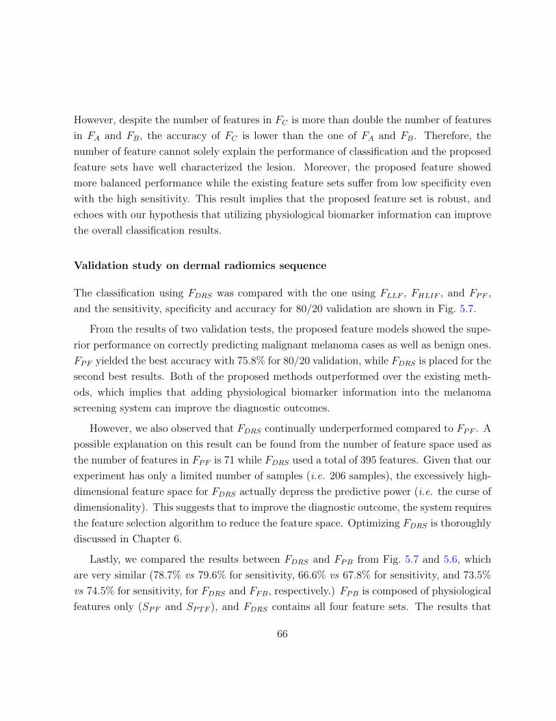
However, despite the number of features in FC is more than double the number of features

in FA and FB, the accuracy of FC is lower than the one of FA and FB. Therefore, the

number of feature cannot solely explain the performance of classification and the proposed

feature sets have well characterized the lesion. Moreover, the proposed feature showed

more balanced performance while the existing feature sets suffer from low specificity even

with the high sensitivity. This result implies that the proposed feature set is robust, and

echoes with our hypothesis that utilizing physiological biomarker information can improve

the overall classification results.

Validation study on dermal radiomics sequence

The classification using FDRS was compared with the one using FLLF , FHLIF , and FPF ,

and the sensitivity, specificity and accuracy for 80/20 validation are shown in Fig. 5.7.

From the results of two validation tests, the proposed feature models showed the supe-

rior performance on correctly predicting malignant melanoma cases as well as benign ones.

FPF yielded the best accuracy with 75.8% for 80/20 validation, while FDRS is placed for the

second best results. Both of the proposed methods outperformed over the existing meth-

ods, which implies that adding physiological biomarker information into the melanoma

screening system can improve the diagnostic outcomes.

However, we also observed that FDRS continually underperformed compared to FPF . A

possible explanation on this result can be found from the number of feature space used as

the number of features in FPF is 71 while FDRS used a total of 395 features. Given that our

experiment has only a limited number of samples (i.e. 206 samples), the excessively high-

dimensional feature space for FDRS actually depress the predictive power (i.e. the curse of

dimensionality). This suggests that to improve the diagnostic outcome, the system requires

the feature selection algorithm to reduce the feature space. Optimizing FDRS is thoroughly

discussed in Chapter 6.

Lastly, we compared the results between FDRS and FPB from Fig. 5.7 and 5.6, which

are very similar (78.7% vs 79.6% for sensitivity, 66.6% vs 67.8% for sensitivity, and 73.5%

vs 74.5% for sensitivity, for FDRS and FFB, respectively.) FPB is composed of physiological

features only (SPF and SPTF ), and FDRS contains all four feature sets. The results that

66

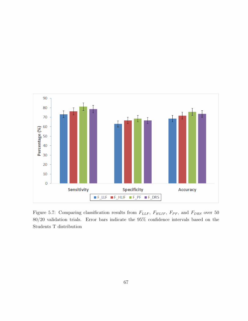
Figure 5.7: Comparing classification results from FLLF , FHLIF , FPF , and FDRS over 50

80/20 validation trials. Error bars indicate the 95% confidence intervals based on the

Students T distribution

67

the difference between two models is very small implies that FPB heavily influences the

decision made by FDRS, and other feature sets (SLLF and SHLIF ) are mostly ignored or the

influence is minimal. This limitation becomes another reason that FDRS requires a proper

feature selection to improve the results, on top of the curse of dimensionality.

5.6 Summary

This chapter has presented the dermal radiomics sequence, which consists of the existing

feature sets based on ABCD-rule, and the novel feature sets. The proposed feature sets

extracted a total of 334 features, which utilizes the spatial heterogeneity as well as ex-

ploring different colour spaces to characterize the skin lesion better. The validation study

showed that the DRS can outperform over the existing sets with the improved results, but

at the same time, the challenge that incurred from the curse of dimensionality. In the

next chapter, we conduct feature analysis on the DRS by examining feature selection and

classification algorithm for improving diagnostic outcome of melanoma.

68

Chapter 6

Feature Analysis for Dermal

Radiomics

6.1 Introduction

In the two previous chapters, the fundamental blocks of dermal radiomics framework have

been discussed. The roles of eumelanin, pheomelanin, and hemoglobin related to melanoma

were explored, and a novel technique to quantify their concentrations was proposed. Based

on these information, the dermal radiomics sequences, which characterizes each skin lesion

with unique 395 features, was designed. This current chapter presents a final process of

dermal radiomics, which is feature analysis. Feature analysis is divided into classifica-

tion analysis and feature selection analysis to find the feature selection and classification

algorithm that works the best with the proposed dermal radiomics sequence.

6.2 Classification Analysis

In this section, different classification algorithms are discussed to find an appropriate clas-

sification algorithm for the dermal radiomics framework. Three classification algorithms

have been examined: random forest classification (RF), support vector machine (SVM),

69

and naive Bayes classification (NB). Random forest classification was a family of ensemble

learning algorithm, and thus, it is well known to handle well on highly non-linear interac-

tions from predictors. SVM and Bayesian classification is one of the most frequently used

classification algorithms for diagnosing melanoma, and have shown the promising results

in many studies [30, 45, 106, 29].

6.2.1 Experimental Design

For the dataset used in this experiment, a total of 206 pre-processed skin lesion images,

which were acquired by standard camera, was used. A detailed explanation of data collec-

tion and pre-processing step can be found in Section 5.5. In short, each skin lesion image

goes through dermal radiomics framework and eventually generates the dermal radiomics

sequence. Each image in the dataset is labeled either malignant or benign as the ground

truth for the classification. Then, the three classification algorithms (RF, SVM, NB) are

examined on the set of dermal radiomics sequence. For RF, the number of trees used for

classification, and the subset of predictor variables used at each node are set at the default

values, and for SVM, quadratic kernel was employed.

To get a comprehensive assessment of classification, an additional measure, which is the

receiver operating characteristic (ROC) curve, was used on top of sensitivity, specificity,

and accuracy. Using only sensitivity, specificity, and accuracy may conclude a biased

decision on highly disproportionate dataset of malignant and benign cases. ROC curve is

the visualization of the classifier’s ability to separate two classes regardless of the proportion

of classes. The ROC curve is a plot of true positive rate (sensitivity) versus false positive

rate (1-specificity) across varying cut-offs, and therefore, the accuracy is determined by

how close the curve follows to the upper-left border of the ROC space (Fig. 6.3).

To calculate the accuracy of each classification method, the leave-one-out cross valida-

tion (LOO) and 80/20 cross validation are employed. Given that n samples for the test,

LOO uses n−1 samples as training data, and the only remaining sample is used for testing.

It iterates n times so that every sample in the data could be used as testing data. 80/20

cross validation uses 80% of the entire dataset as training data, which is randomly chosen

70

at each iteration, and the remaining 20% is used as testing data. In this validation study,

50 trials of 80/20 cross validation are performed.

Figure 6.1: 80/20 cross validation: The sensitivity, specificity, and accuracy of RF, SVM,

and NB classification are reported. Error bars indicate the 95% confidence intervals based

on the Students T distribution.

6.2.2 Results

Fig. 6.1 and 6.2 shows sensitivity, specificity and accuracy of all testing classification al-

gorithms, which was performed using the dermal radiomics sequence. From 80/20 cross

validation, RF outperformed over other methods by yielding 85.0% of sensitivity, 72.7% of

specificity, and 79.3% of accuracy. Similar trend was observed in the LOO cross validation

results. Moreover, from ROC curve shown in Fig. 6.3, RF (in blue) performs better than

SVM (in red) and NB (in green) in most of time, and the area under curve (AUC), which

measures the performance of ROC curve as a quantitative value, for RF, SVM and NB are

reported as 0.87, 0.83, and 0.75, respectively. From these results, it shows that RF is well

suited for dermal radiomics framework, and thus, RF classification algorithm are employed

71

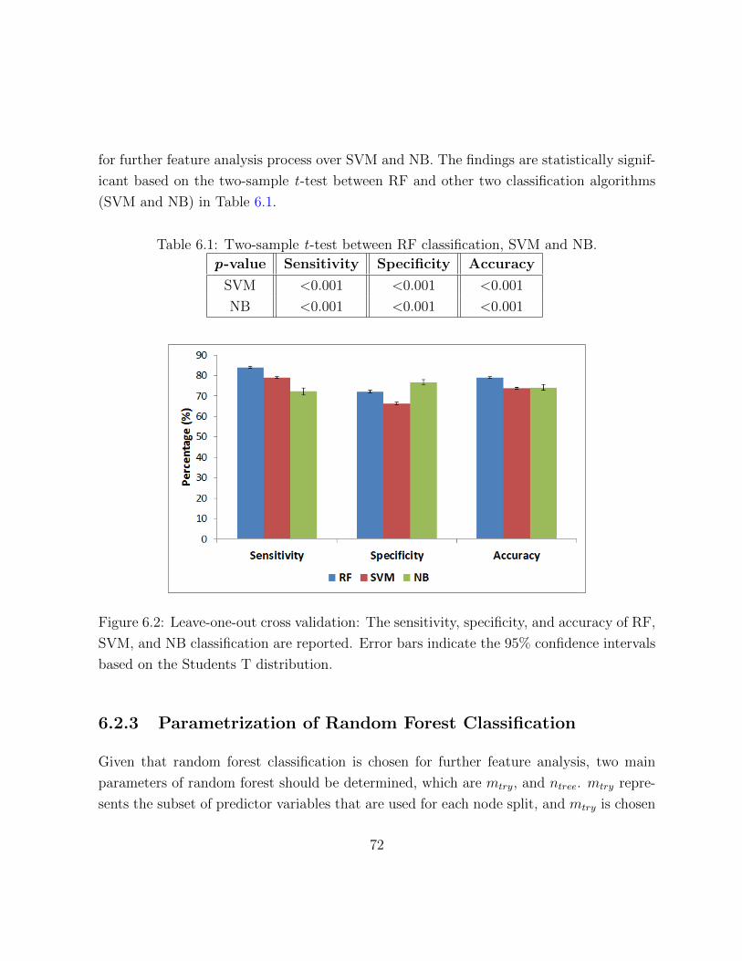
for further feature analysis process over SVM and NB. The findings are statistically signif-

icant based on the two-sample t-test between RF and other two classification algorithms

(SVM and NB) in Table 6.1.

Table 6.1: Two-sample t-test between RF classification, SVM and NB.

p-value Sensitivity Specificity Accuracy

SVM <0.001 <0.001 <0.001

NB <0.001 <0.001 <0.001

Figure 6.2: Leave-one-out cross validation: The sensitivity, specificity, and accuracy of RF,

SVM, and NB classification are reported. Error bars indicate the 95% confidence intervals

based on the Students T distribution.

6.2.3 Parametrization of Random Forest Classification

Given that random forest classification is chosen for further feature analysis, two main

parameters of random forest should be determined, which are mtry, and ntree. mtry repre-

sents the subset of predictor variables that are used for each node split, and mtry is chosen

72

Figure 6.3: ROC for RF, SVM, and NB classification

randomly at the node. The default value for the number of mtry is√k for classification,

and k/3 for regression, where k is the number of entire predictor variables. ntree is the

number of classifier generated, and the default value is 500. In this section, mtry and ntree

are parametrized to optimize the performance of random forest for dermal radiomics.

Parametrization for mtry

For the search of mtry, three different values have been tested: 1)√k, 2) k/3, and 3) 6.

The value of six was chosen because the default value of mtry is six when top 10% rank

on DRS was used. Therefore, instead of varying mtry for different feature model, the value

was fixed as six for consistency. 50 80/20 validation trials were performed on DRS, and

the evaluation results were reported in Table 6.2.

As shown in Table. 6.2, the changes between different mtry are very small that any

choice of mtry would not influence the results greatly. However, some variation are found

in time executed between k/3 and other two that the choice of k/3 took longer to execute.

73

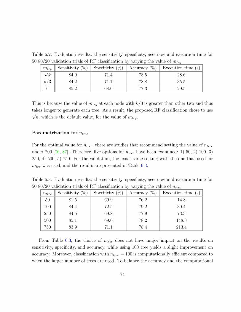
Table 6.2: Evaluation results: the sensitivity, specificity, accuracy and execution time for

50 80/20 validation trials of RF classification by varying the value of mtry.

mtry Sensitivity (%) Specificity (%) Accuracy (%) Execution time (s)√k 84.0 71.4 78.5 28.6

k/3 84.2 71.7 78.8 35.5

6 85.2 68.0 77.3 29.5

This is because the value of mtry at each node with k/3 is greater than other two and thus

takes longer to generate each tree. As a result, the proposed RF classification chose to use√k, which is the default value, for the value of mtry.

Parametrization for ntree

For the optimal value for ntree, there are studies that recommend setting the value of ntree

under 200 [76, 87]. Therefore, five options for ntree have been examined: 1) 50, 2) 100, 3)

250, 4) 500, 5) 750. For the validation, the exact same setting with the one that used for

mtry was used, and the results are presented in Table 6.3.

Table 6.3: Evaluation results: the sensitivity, specificity, accuracy and execution time for

50 80/20 validation trials of RF classification by varying the value of ntreentree Sensitivity (%) Specificity (%) Accuracy (%) Execution time (s)

50 81.5 69.9 76.2 14.8

100 84.4 72.5 79.2 30.4

250 84.5 69.8 77.9 73.3

500 85.1 69.0 78.2 148.3

750 83.9 71.1 78.4 213.4

From Table 6.3, the choice of ntree does not have major impact on the results on

sensitivity, specificity, and accuracy, while using 100 tree yields a slight improvement on

accuracy. Moreover, classification with ntree = 100 is computationally efficient compared to

when the larger number of trees are used. To balance the accuracy and the computational

74

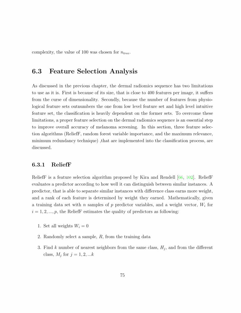
complexity, the value of 100 was chosen for ntree.

6.3 Feature Selection Analysis

As discussed in the previous chapter, the dermal radiomics sequence has two limitations

to use as it is. First is because of its size, that is close to 400 features per image, it suffers

from the curse of dimensionality. Secondly, because the number of features from physio-

logical feature sets outnumbers the one from low level feature set and high level intuitive

feature set, the classification is heavily dependent on the former sets. To overcome these

limitations, a proper feature selection on the dermal radiomics sequence is an essential step

to improve overall accuracy of melanoma screening. In this section, three feature selec-

tion algorithms (ReliefF, random forest variable importance, and the maximum relevance,

minimum redundancy technique) ,that are implemented into the classification process, are

discussed.

6.3.1 ReliefF

ReliefF is a feature selection algorithm proposed by Kira and Rendell [66, 102]. ReliefF

evaluates a predictor according to how well it can distinguish between similar instances. A

predictor, that is able to separate similar instances with difference class earns more weight,

and a rank of each feature is determined by weight they earned. Mathematically, given

a training data set with n samples of p predictor variables, and a weight vector, Wi for

i = 1, 2, ..., p, the ReliefF estimates the quality of predictors as following:

1. Set all weights Wi = 0

2. Randomly select a sample, R, from the training data

3. Find k number of nearest neighbors from the same class, Hj, and from the different

class, Mj for j = 1, 2, ...k

75

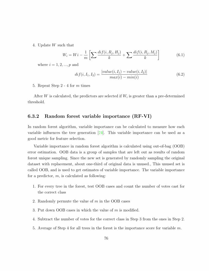
4. Update W such that

Wi = Wi− 1

m

[∑ dif(i, Rj, Hj)

k+∑ dif(i, Rj,Mj)

k

](6.1)

where i = 1, 2, ..., p and

dif(i, I1, I2) =|value(i, I1)− value(i, I2)|

max(i)−min(i)(6.2)

5. Repeat Step 2 - 4 for m times

After W is calculated, the predictors are selected if Wi is greater than a pre-determined

threshold.

6.3.2 Random forest variable importance (RF-VI)

In random forest algorithm, variable importance can be calculated to measure how each

variable influences the tree generation [24]. This variable importance can be used as a

good metric for feature selection.

Variable importance in random forest algorithm is calculated using out-of-bag (OOB)

error estimation. OOB data is a group of samples that are left out as results of random

forest unique sampling. Since the new set is generated by randomly sampling the original

dataset with replacement, about one-third of original data is unused., This unused set is

called OOB, and is used to get estimates of variable importance. The variable importance

for a predictor, m, is calculated as following:

1. For every tree in the forest, test OOB cases and count the number of votes cast for

the correct class

2. Randomly permute the value of m in the OOB cases

3. Put down OOB cases in which the value of m is modified.

4. Subtract the number of votes for the correct class in Step 3 from the ones in Step 2.

5. Average of Step 4 for all trees in the forest is the importance score for variable m.

76

6.3.3 Maximum Relevance, Minimum Redundancy Technique

The maximum relevance, minimum redundancy technique (mRMR) was introduced by

Peng et. al [94], and it find the feature which has maximal relevance and minimal redun-

dancy. Maximal relevance is a process of finding a feature with the highest relevance to

the target class, while minimal redundancy find a feature that maximize the joint depen-

dency of features on the target class to reduce redundancy among features. mRMR uses

a heuristic search algorithm to satisfy both maximal relevance and minimal redundancy.

Mathematically, relevance and redundancy of feature subset is defined as follows:

V (i, h) =1

|F |∑i∈F

I(i, h) (6.3)

W (i) =1

|F |2∑i,j∈F

I(i, j) (6.4)

where Fm is a feature subset, h is the target class, i, j is features, and I(·) is the mu-

tual information function. V and W are the relevance and redundancy of feature set,

respectively. The best feature subset, is found using greedy search algorithm to satisfy the

following criteria:

max Φ(V,W ), Φ = V −W (6.5)

6.3.4 Experimental Design

In this experiment, three features selection methods were validated: mRMR, ReliefF and

RF-VI. The experimental setup is exactly the same as the one used in classification analysis.

Each method runs through the training dataset and ranks each predictor variable from the

most influence one to the least. Then, random forest classification was employed on the

subset of dermal radiomics sequences, and the number of feature used increased from 5 to

385 with a step of 10. To measure the accuracy of the testing feature selection algorithms,

LOO cross validation and 50 trials of 80/20 cross validation were conducted.

77

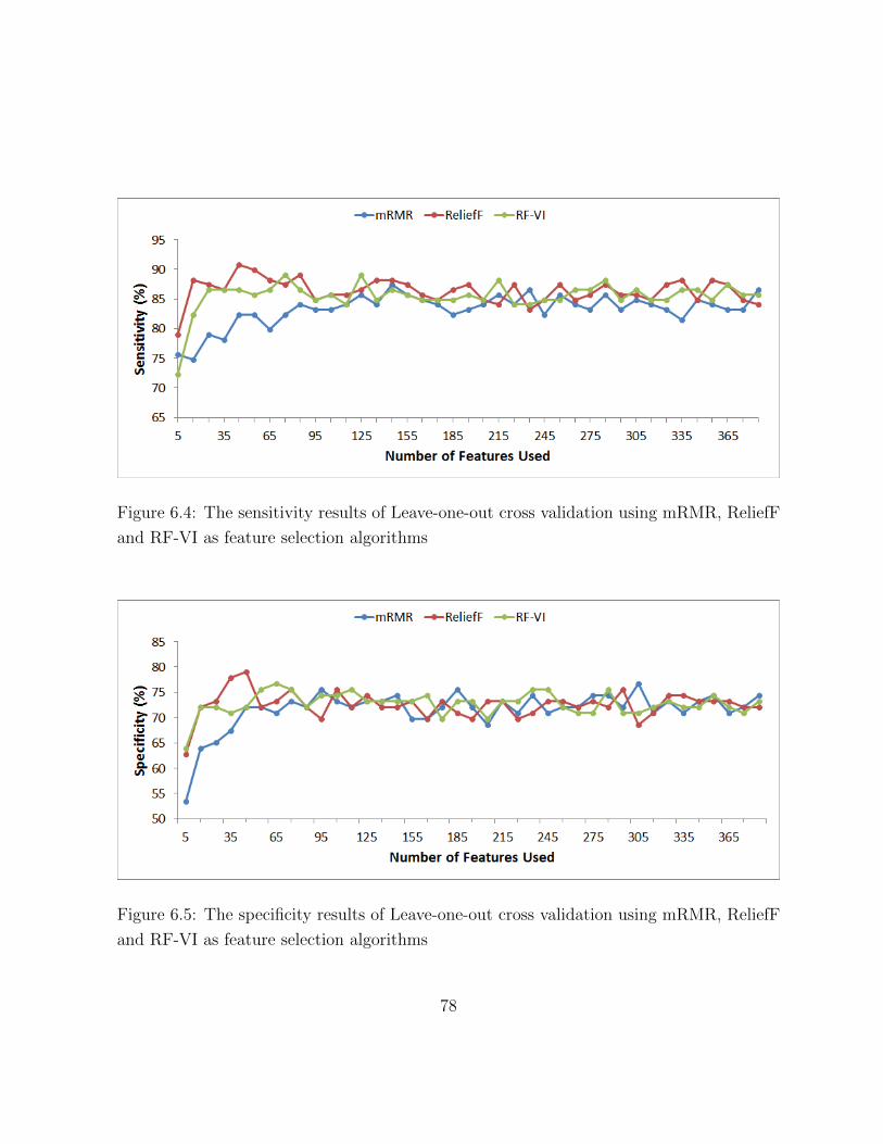
Figure 6.4: The sensitivity results of Leave-one-out cross validation using mRMR, ReliefF

and RF-VI as feature selection algorithms

Figure 6.5: The specificity results of Leave-one-out cross validation using mRMR, ReliefF


78

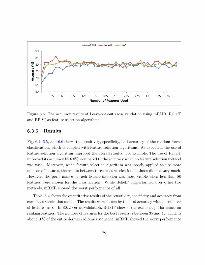
Figure 6.6: The accuracy results of Leave-one-out cross validation using mRMR, ReliefF


6.3.5 Results

Fig. 6.4, 6.5, and 6.6 shows the sensitivity, specificity, and accuracy of the random forest

classification, which is coupled with feature selection algorithms. As expected, the use of

feature selection algorithm improved the overall results. For example, The use of ReliefF

improved its accuracy by 6.8%, compared to the accuracy when no feature selection method

was used. Moreover, when feature selection algorithm was loosely applied to use more

number of features, the results between three feature selection methods did not vary much.

However, the performance of each feature selection was more visible when less than 80

features were chosen for the classification. While ReliefF outperformed over other two

methods, mRMR showed the worst performance of all.

Table. 6.4 shows the quantitative results of the sensitivity, specificity and accuracy from

each feature selection model. The results were chosen by the best accuracy with the number

of features used. In 80/20 cross validation, ReliefF showed the excellent performance on

ranking features. The number of features for the best results is between 35 and 45, which is

about 10% of the entire dermal radiomics sequence. mRMR showed the worst performance

79

of all three testing feature selection algorithms. The number of features used to yield the

best accuracy is 145, and mRMR did not work well on optimizng the DRS when compared

to ReliefF algorithm.

Table 6.4: 50 trials of 80/20 cross validation results for melanoma detection: Compar-

ing feature selection models (ReliefF, RF-VI and mRMR) on sensitivity, specificity, and

accuracy(%). Results are shown with 95% confidence interval.

Feature selection

method

Number of

featuresSensitivity Specificity Accuracy

ReliefF 35 88.8 [87.2 90.4] 77.9 [74.9 80.8] 84.1 [82.7 85.5]

RF-VI 75 85.8 [83.8 87.8] 72.9 [69.8 76.0] 80.2 [78.7 81.7]

mRMR 170 83.3 [81.4 85.3] 71.7 [68.9 74.5] 78.4 [76.7 80.1]

Another classification metric was used to examine the performance of feature selection

aglorithm. A receiver operating characteristic (ROC) curve was computed in Fig. 6.7. The

results from ROC curve also agree with our findings above as area under curve (AUC) for

ROC is 0.91, 0.88, and 0.85 for ReliefF, RF-VI, and mRMR, respectively.

Lastly, the ranked features are examined to see how each feature are contributed to

overall classification results. Among 35 highly ranked features by ReliefF feature selection

algorithm, 9 features are from low level feature set. More specifically, four of nine describes

asymmetry, three and two features describe color variation and differential structure of

lesion, respectively. Two features, which describes irregularity of lesion, are from high

level intuitive feature set. Moreover, mean and variance of eumelanin and hemoglobin

are ranked as the most important features from physiological feature set. Lastly, a total

of 20 features are highly ranked from physiological texture feature set for classification.

Nine, six, and five features are derived from eumelanin, Pheomelanin, and hemoglobin,

respectively.

Given that the majority of dermal radiomics sequence is made up by physiological

texture feature set, a 35 highly ranked features have well-balanced mixture of each fea-

ture set: 11 features are obtained from LLF and HLIF, and 24 are from PT and PTF. It

reflects that the proposed dermal radiomics, which is composed of the feature set based

80

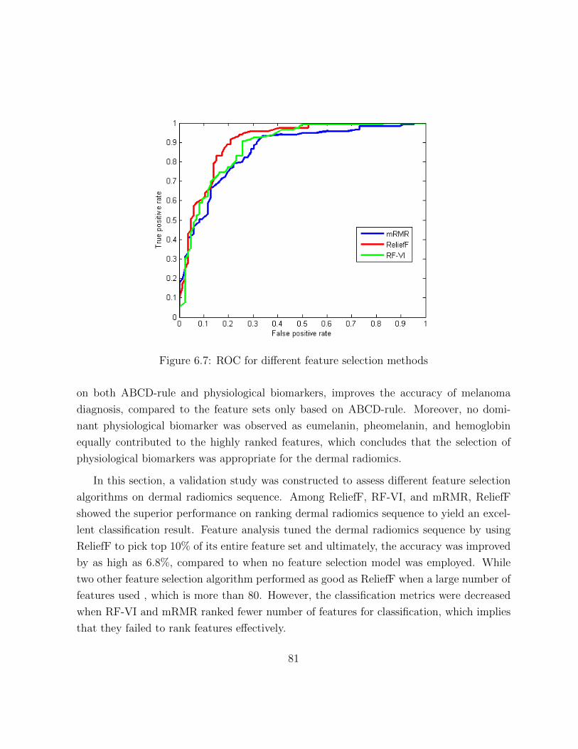
Figure 6.7: ROC for different feature selection methods

on both ABCD-rule and physiological biomarkers, improves the accuracy of melanoma

diagnosis, compared to the feature sets only based on ABCD-rule. Moreover, no domi-

nant physiological biomarker was observed as eumelanin, pheomelanin, and hemoglobin

equally contributed to the highly ranked features, which concludes that the selection of

physiological biomarkers was appropriate for the dermal radiomics.

In this section, a validation study was constructed to assess different feature selection

algorithms on dermal radiomics sequence. Among ReliefF, RF-VI, and mRMR, ReliefF

showed the superior performance on ranking dermal radiomics sequence to yield an excel-

lent classification result. Feature analysis tuned the dermal radiomics sequence by using

ReliefF to pick top 10% of its entire feature set and ultimately, the accuracy was improved

by as high as 6.8%, compared to when no feature selection model was employed. While

two other feature selection algorithm performed as good as ReliefF when a large number of

features used , which is more than 80. However, the classification metrics were decreased

when RF-VI and mRMR ranked fewer number of features for classification, which implies

that they failed to rank features effectively.

81

6.4 Validation study on dermal radiomics

From the feature analysis, the random forest classification and reliefF were selected as the

classification and feature selection algorithm for dermal radiomics framework. To validate

the complete dermal radiomics, it was compared with the state-of-the-art computer-aided

melanoma diagnosis as well as the conventional diagnosis of dermatologists.

6.4.1 Comparison with the state-of-the-art techniques

Given that the proposed dermal radiomics use the standard camera imaging modality in-

stead of dermascopic images, the two state-of-the-art computer-aided melanoma screening

systems, which are also uses the dermal images, are chosen for comparison. The first

melanoma screening system was adapted from Cavalcanti et al. [28]. They designed fea-

tures which describes ABCD-rule using mathematical formulation, and the feature set they

designed are adapted into dermal radiomics sequence as low level feature. The next state-

of-the-art technique was developed by Amelard et. al. [3], and they constructed high level

intuitive features based on ABCD-rule as well. The melanoma screening for this group

was performed based on the feature set, which combined their novel features as well as low

level features. For the validation, 50 trials of 80/20 cross validation study was performed

on the proposed dermal radiomics sequence as well as two state-of-the-art techniques, and

the feature model for each technique is defined as follows:

• FLLF = SLLF

• FHLIF = SLLF ∪ SHLIF

• FDRS = SLLF ∪ SHLIF ∪ SPF ∪ SPTF

The sensitivity, specificity and accuracy of the state-of-the-art techniques as well as

proposed dermal radiomics, which are obtained from feature analysis, are presented in

Table 6.5. For comparison, the result table from Section 5.5.5 was adapted in Table 6.6.

82

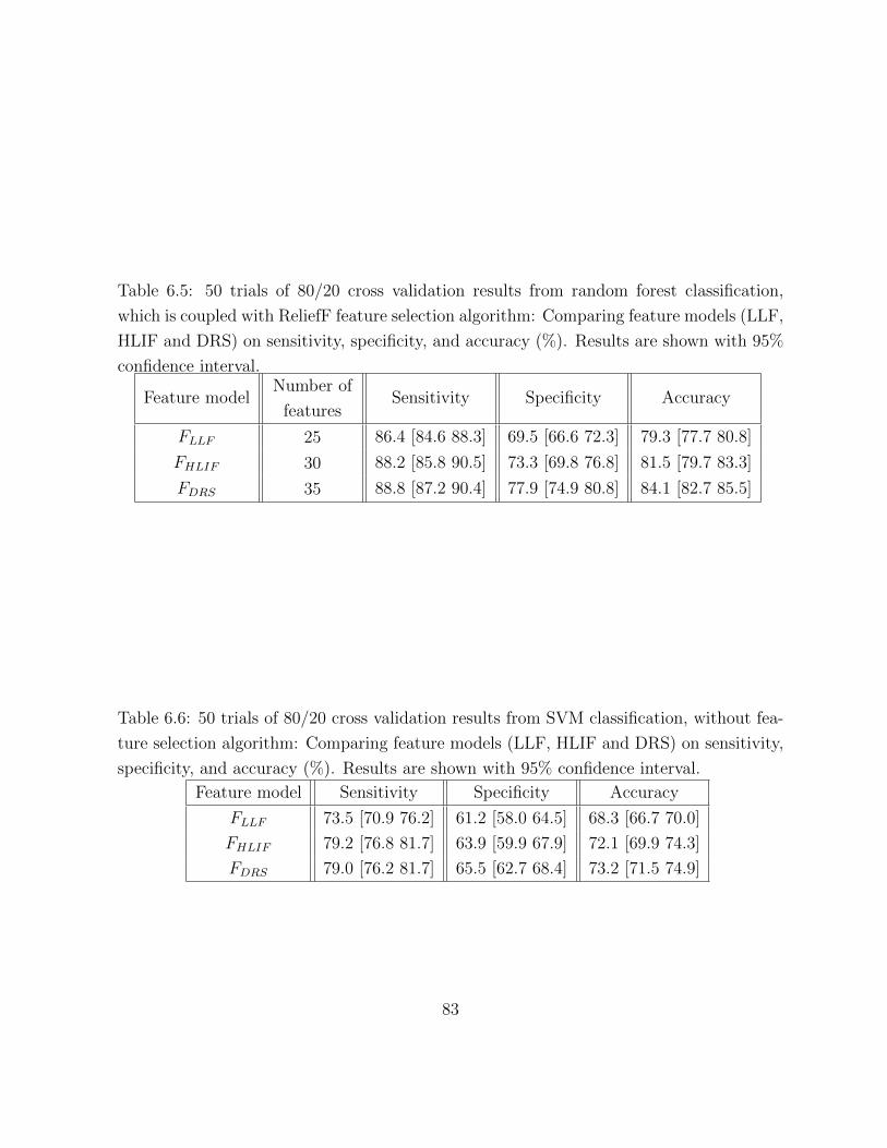
Table 6.5: 50 trials of 80/20 cross validation results from random forest classification,

which is coupled with ReliefF feature selection algorithm: Comparing feature models (LLF,

HLIF and DRS) on sensitivity, specificity, and accuracy (%). Results are shown with 95%

confidence interval.

Feature modelNumber of

featuresSensitivity Specificity Accuracy

FLLF 25 86.4 [84.6 88.3] 69.5 [66.6 72.3] 79.3 [77.7 80.8]

FHLIF 30 88.2 [85.8 90.5] 73.3 [69.8 76.8] 81.5 [79.7 83.3]

FDRS 35 88.8 [87.2 90.4] 77.9 [74.9 80.8] 84.1 [82.7 85.5]

Table 6.6: 50 trials of 80/20 cross validation results from SVM classification, without fea-

ture selection algorithm: Comparing feature models (LLF, HLIF and DRS) on sensitivity,

specificity, and accuracy (%). Results are shown with 95% confidence interval.

Feature model Sensitivity Specificity Accuracy

FLLF 73.5 [70.9 76.2] 61.2 [58.0 64.5] 68.3 [66.7 70.0]

FHLIF 79.2 [76.8 81.7] 63.9 [59.9 67.9] 72.1 [69.9 74.3]

FDRS 79.0 [76.2 81.7] 65.5 [62.7 68.4] 73.2 [71.5 74.9]

83

In Table 6.5 and 6.6, classification results were compared with/without feature analysis.

the proposed dermal radiomics sequence, FDRS, showed an inferior performance in Table

6.6 when the entire feature set was used for classification. However, the vast improvement

on all classification metrics including sensitivity, specificity and accuracy was observed with

the use of feature analysis. Moreover, not only the results from FDRS was improved but

also the results from all other feature models were increased when the appropriate feature

selection and classification algorithm were applied. From the statistical significant testing,

the superior performance of the proposed method are statistically significant on specificity

and accuracy (Table 6.7).

Table 6.7: Two-sample t-test between the dermal radiomics and the state-of-the-art tech-

niques.

p-value Sensitivity Specificity Accuracy

LLF 0.057 <0.001 <0.001

HLIF 0.656 0.045 0.022

6.4.2 Comparison with conventional diagnosis

The complete dermal radiomics was compared with the current diagnostic practice of der-

matologists. Given that it is not possible to compare the accuracy directly because no

diagnosis from dermatologists was made in the same setting in which the dataset was

collected, the sensitivity and specificity were compared based on the report from the lit-

erature. Two studies were found in terms of the melanoma diagnosis: 1) dermatologists

conducted diagnosis of melanoma in the clinical setting by directly contacting patients and

2) dermatologists diagnose based on the dermal images only. While the proposed dermal

radiomics exhibits 88.7% of sensitivity and 78.6% of specificity, dermatologists experience

71% of sensitivity and 81% of specificity when diagnosing on site [130] , and 98.1% of sen-

sitivity and 30.4% of specificity when diagnosing based on images [132]. The results shows

that the proposed method provides more reliable and robust diagnosis on melanoma. Espe-

cially, when dermatologists used the image only for making diagnostic decision, it yielded

84

high sensitivity but the specificity was dismal. The balanced results from the dermal ra-

diomics make the proposed framework more suitable for a tele-medicine tool, for which the

diagnosis based on images is greatly appreciated.

6.5 Summary

This chapter has presented the random forest classification for dermal radiomics frame-

work. To optimize the performance of random forest classification, the parametrization

was conducted, and the feature selection algorithm was integrated into the classification.

Moreover, a series of validation study was conducted to assess the proposed dermal ra-

diomics sequence and the classification algorithm against the existing ones. The results

showed that the random forest using DRS can yield superior performance, which implies

that the proposed dermal radiomics can aid dermatologists and general practitioners to

improve their melanoma diagnostic outcomes.

85

Chapter 7

Conclusions

In this chapter, the summary of research contributions is provided followed by a few sug-

gestions for the directions of future research.

7.1 Summary of Contributions

The specific contributions in the three main chapters of this thesis are described as follow-

ing.

• In Chapter 3 and 4, a novel physiological biomarker extraction technique for a skin

lesion is proposed. Given that melanoma is the results of uncontrollable production

of melanin, utilizing melanin concentrations as well as hemoglobin may provide addi-

tional insights on melanoma diagnosis. Under the current diagnosis of melanoma, skin

lesions are typically acquired by standard camera, and the physiological biomarker

information are not directly available from these images. Moreover, most state-

of-the-art techniques for physiological biomarker extraction simplifies the light-skin

interaction, that only accounts for absorption only. The proposed method is de-

signed to extract the concentrations of eumelanin, pheomelanin, and hemoglobin as

an inverse function of the complex light-skin interaction model, which accounts for

reflection, scattering and absorption between various interface of skin layers.

86

• In Chapter 5, the dermal radiomics sequence is constructed. While most computer-

aided melanoma screening system employs features based on ABCD-rule, the pro-

posed radiomics sequence includes not only feature sets, which are based on ABCD-

rule, but also utilizes the physiological biomarker information, which was obtained in

Chapter 3. A complete dermal radiomics sequence consists of four feature sets. First

two feature sets are low level feature, and high level intuitive feature, which quantify

ABCD criteria of the skin lesion. The last two feature sets are based on the concen-

trations of eumelanin, pheomelanin, and hemoglobin. These sets measures spatial

heterogeneity of physiological biomarkers and the texture information of lesion using

six different colour spaces. Ultimately, dermal radiomics sequence generated a total

of 395 features to thoroughly characterize each skin lesion.

• In Chapter 6, feature analysis for the proposed dermal radiomics framework is con-

ducted. First, classification analysis is performed to find an appropriate classifica-

tion algorithm for dermal radiomics. Three classification algorithms (random forest,

support vector machine, naive Bayes classification), which are widely employed for

melanoma classification, are compared. From the validation study, the random forest

classification showed the superior performance on diagnosing melanoma over other

two methods. Second, feature selection analysis is conducted to optimize the use of

dermal radiomics sequence. Different feature selection algorithms are explored and

ReliefF is chosen for the dermal radiomics as it yields the best sensitivity, specificity

and accuracy. From the feature analysis, the most effective feature selection and

classification algorithm for the dermal radiomics are chosen.

7.2 Future Research

The work motivates future research in the following directions.

• We extracted the concentrations of eumelanin, pheomelanin, and hemoglobin by using

the physiological biomarker extraction in Chapter 3. While we used this technique

for skin cancer research, this can be further extended into skin colour reproduction

87

technique. In skin colour reproduction technique, melanin and hemoglobin plays

important roles for reproducing facial skin colour. It is reported that the melanin

texture of a 50 year-old woman is different than the texture of a 20 year-old woman.

Moreover, the level of hemoglobin changes due to alcohol consumption or tanning.

By measuring concentrations of melanin and hemoglobin accurately, more realistic

skin colour can be reproduced.

• The proposed melanoma screening system diagnoses either benign or malignant

melanoma, which is binary classification. As mentioned in Chapter 2, there are

four subtypes of melanoma, and treatment option could be different based on which

type of melanoma the patient has. Therefore, our system can be further investigated

to include multi-class classification. The only limitation on our study is that we did

not have sufficient image data to fully characterize each subtype of melanoma. It

would be a good direction to take if we can further analyze dermal radiomics se-

quence so that the random forest classification can diagnose subtypes of melanoma.

Moreover, not only the subtype of melanoma, but also other types of skin cancer

can be classified using the proposed screening system. While non-melanoma skin

cancer is not dangerous compared to melanoma, Merkel cell carcinoma requires more

attention because this type of cancer is not easily diagnosed in the early stage of

cancer.

• For the more accurate measurement of physiological biomarker concentrations, multi-

spectral imaging could be employed. This could be especially beneficial if oxygenated

hemoglobin and deoxygenated hemoglobin needs to be separated. Moreover, eume-

lanin and pheomelanin exhibits different spectral responses in near infra-red fre-

quency domain, thus, the multi-spectral imaging can provide an improved measure-

ment on physiological biomarkers.

• Another area of future research would be to wrap this entire melanoma screening

system into mobile application. This can help potentially those who live in remote

area, and the access to clinicians or dermatologists is limited. Moreover, this will

promote self-examination of melanoma and can lead to early detection of this type

of skin cancer. As mentioned in Chapter 2, even though melanoma has high incident

88

rate, the mortality rate is relatively low because of early detection. Mobile application

of melanoma screening system can further reduce the mortality rate.

89

References

[1] Naheed R Abbasi, Helen M Shaw, Darrell S Rigel, Robert J Friedman, William H Mc-

Carthy, Iman Osman, Alfred W Kopf, and David Polsky. Early diagnosis of cutaneous

melanoma. JAMA: the journal of the American Medical Association, 292(22):2771–

2776, 2004.

[2] Hugo JWL Aerts, Emmanuel Rios Velazquez, Ralph TH Leijenaar, Chintan Parmar,

Patrick Grossmann, Sara Carvalho, Johan Bussink, Rene Monshouwer, Benjamin

Haibe-Kains, Derek Rietveld, et al. Decoding tumour phenotype by noninvasive

imaging using a quantitative radiomics approach. Nature communications, 5, 2014.

[3] Robert Amelard, Alexander Wong, and David A Clausi. Extracting morphological

high-level intuitive features (hlif) for enhancing skin lesion classification. In Engineer-

ing in Medicine and Biology Society (EMBC), 2012 Annual International Conference

of the IEEE, pages 4458–4461. IEEE, 2012.

[4] Elli Angelopoulou. Understanding the color of human skin. In Photonics West 2001-

Electronic Imaging, pages 243–251. International Society for Optics and Photonics,

2001.

[5] Giuseppe Argenziano, H Peter Soyer, Sergio Chimenti, Renato Talamini, Rosamaria

Corona, Francesco Sera, Michael Binder, Lorenzo Cerroni, Gaetano De Rosa, Gerardo

Ferrara, et al. Dermoscopy of pigmented skin lesions: results of a consensus meeting

via the internet. Journal of the American Academy of Dermatology, 48(5):679–693,

2003.

90

[6] BK Armstrong, A Kricker, and DR English. Sun exposure and skin cancer. The

Australasian journal of dermatology, 38:S1, 1997.

[7] Bruce K Armstrong and Anne Kricker. The epidemiology of uv induced skin cancer.

Journal of Photochemistry and Photobiology B: Biology, 63(1):8–18, 2001.

[8] Paolo Ascierto, Marco Palla, Fabrizio Ayala, Ileana De Michele, Corrado Caraco,

Antonio Daponte, Ester Simeone, Stefano Mori, Maurizio Del Giudice, Rocco Sa-

triano, et al. The role of spectrophotometry in the diagnosis of melanoma. BMC

dermatology, 10(1):5, 2010.

[9] Tjeerd S Aukema, Renato A Valdes Olmos, Catharina M Korse, Bin BR Kroon,

Michel WJM Wouters, Wouter V Vogel, Johannes MG Bonfrer, and Omgo E Nieweg.

Utility of fdg pet/ct and brain mri in melanoma patients with increased serum s-100b

level during follow-up. Annals of surgical oncology, 17(6):1657–1661, 2010.

[10] Marie-Lise Bafounta, Alain Beauchet, Sophie Chagnon, and Philippe Saiag. Ultra-

sonography or palpation for detection of melanoma nodal invasion: a meta-analysis.

The lancet oncology, 5(11):673–680, 2004.

[11] Charles M Balch, Antonio C Buzaid, Seng-Jaw Soong, Michael B Atkins, Natale

Cascinelli, Daniel G Coit, Irvin D Fleming, Jeffrey E Gershenwald, Alan Houghton,

John M Kirkwood, et al. Final version of the american joint committee on cancer

staging system for cutaneous melanoma. Journal of Clinical Oncology, 19(16):3635–

3648, 2001.

[12] Charles M Balch, Jeffrey E Gershenwald, Seng-jaw Soong, John F Thompson,

Michael B Atkins, David R Byrd, Antonio C Buzaid, Alistair J Cochran, Daniel G

Coit, Shouluan Ding, et al. Final version of 2009 ajcc melanoma staging and classi-

fication. Journal of clinical oncology, 27(36):6199–6206, 2009.

[13] Charles M Balch, Seng-Jaw Soong, Jeffrey E Gershenwald, John F Thompson, Dou-

glas S Reintgen, Natale Cascinelli, Marshall Urist, Kelly M McMasters, Merrick I

Ross, John M Kirkwood, et al. Prognostic factors analysis of 17,600 melanoma

91

patients: validation of the american joint committee on cancer melanoma staging

system. Journal of Clinical Oncology, 19(16):3622–3634, 2001.

[14] Jeremy P Banky, John W Kelly, Dallas R English, Josephine M Yeatman, and John P

Dowling. Incidence of new and changed nevi and melanomas detected using baseline

images and dermoscopy in patients at high risk for melanoma. Archives of derma-

tology, 141(8):998, 2005.

[15] Gladimir VG Baranoski and Aravind Krishnaswamy. Light and Skin Interactions:

Simulations for Computer Graphics Applications. Morgan Kaufmann, 2010.

[16] Gladimir VG Baranoski and Jon G Rokne. An algorithmic reflectance and trans-

mittance model for plant tissue. In Computer Graphics Forum, volume 16, pages

C141–C150. Wiley Online Library, 1997.

[17] Agop Y Bedikian, Sewa S Legha, Giora Mavligit, Cesar H Carrasco, Sunil Kho-

rana, Carl Plager, Nicholas Papadopoulos, and Robert S Benjamin. Treatment of

uveal melanoma metastatic to the liver. a review of the md anderson cancer center

experience and prognostic factors. Cancer, 76(9):1665–1670, 1995.

[18] Colin B Begg and Marianne Berwick. A note on the estimation of relative risks of

rare genetic susceptibility markers. Cancer Epidemiology Biomarkers & Prevention,

6(2):99–103, 1997.

[19] EG Bendit and D Ross. A technique for obtaining the ultraviolet absorption spectrum

of solid keratin. Applied Spectroscopy, 15(4):103–105, 1961.

[20] Marianne Berwick. Melanoma Epidemiology, chapter 3, pages 35–55. Springer-

Verlag/Wien, 2011.

[21] Alan S Boyd, Yu Shyr, and Lloyd E King Jr. Basal cell carcinoma in young women:

an evaluation of the association of tanning bed use and smoking. Journal of the

American Academy of Dermatology, 46(5):706–709, 2002.

[22] Porcia T Bradford, William F Anderson, Mark P Purdue, Alisa M Goldstein,

and Margaret A Tucker. Rising melanoma incidence rates of the trunk among

92

younger women in the united states. Cancer Epidemiology Biomarkers & Prevention,

19(9):2401–2406, 2010.

[23] Leo Breiman. Bagging predictors. Machine learning, 24(2):123–140, 1996.

[24] Leo Breiman. Random forests. Machine learning, 45(1):5–32, 2001.

[25] Alexander Breslow. Thickness, cross-sectional areas and depth of invasion in the

prognosis of cutaneous melanoma. Annals of surgery, 172(5):902, 1970.

[26] Wiel AG Bruls and Jan C Van Der Leun. Forward scattering properties of human

epidermal layers. Photochemistry and photobiology, 40(2):231–242, 1984.

[27] Canadian Cancer Society Advisory Committee on Cancer Statis-

tics. Canadian Cancer Statistics 2013. http://www.cancer.ca/~/

media/cancer.ca/CW/publications/Canadian%20Cancer%20Statistics/

canadian-cancer-statistics-2013-EN.pdf, 2013. [Online; accessed 10-October-

2013].

[28] Pablo G Cavalcanti and Jacob Scharcanski. Automated prescreening of pigmented

skin lesions using standard cameras. Computerized Medical Imaging and Graphics,

35(6):481–491, 2011.

[29] Pablo G Cavalcanti, Jacob Scharcanski, and Gladimir VG Baranoski. A two-stage

approach for discriminating melanocytic skin lesions using standard cameras. Expert

Systems with Applications, 40(10):4054–4064, 2013.

[30] M Emre Celebi, Hassan A Kingravi, Bakhtiyar Uddin, Hitoshi Iyatomi, Y Alp Aslan-

dogan, William V Stoecker, and Randy H Moss. A methodological approach to the

classification of dermoscopy images. Computerized Medical Imaging and Graphics,

31(6):362–373, 2007.

[31] Miles R Chedekel, Susan K Smith, Peter W Post, Alex Pokora, and David L Ves-

sell. Photodestruction of pheomelanin: role of oxygen. Proceedings of the National

Academy of Sciences, 75(11):5395–5399, 1978.

93

http://www.cancer.ca/~/media/cancer.ca/CW/publications/Canadian%20Cancer%20Statistics/canadian-cancer-statistics-2013-EN.pdf



[32] Lynda Chin. The genetics of malignant melanoma: lessons from mouse and man.

Nature Reviews Cancer, 3(8):559–570, 2003.

[33] Daniel S Cho, Shahid Haider, Robert Amelard, Alexander Wong, and David A Clausi.

Physiological characterization of skin lesion using non-linear random forest regression

model. In Engineering in Medicine and Biology Society (EMBC), 2014 36th Annual

International Conference of the IEEE, pages 3349–3352. IEEE, 2014.

[34] Wallace H Clark, Lynn From, Evelina A Bernardino, and Martin C Mihm. The

histogenesis and biologic behavior of primary human malignant melanomas of the

skin. Cancer research, 29(3):705–727, 1969.

[35] Corinna Cortes and Vladimir Vapnik. Support-vector networks. Machine learning,

20(3):273–297, 1995.

[36] Symon Cotton and Ela Claridge. Developing a predictive model of human skin

coloring. In Medical Imaging 1996, pages 814–825. International Society for Optics

and Photonics, 1996.

[37] JB Dawson, DJ Barker, DJ Ellis, JA Cotterill, E Grassam, GW Fisher, and

JW Feather. A theoretical and experimental study of light absorption and scattering

by in vivo skin. Physics in medicine and biology, 25(4):695, 1980.

[38] Greg R Day and Robert H Barbour. Automated melanoma diagnosis: where are we

at? Skin Research and Technology, 6(1):1–5, 2000.

[39] Sofie AE De Hertog, Christianne AH Wensveen, Maarten T Bastiaens, Christine J

Kielich, Marjo JP Berkhout, Rudi GJ Westendorp, Bert J Vermeer, Jan N Bouwes

Bavinck, et al. Relation between smoking and skin cancer. Journal of Clinical

Oncology, 19(1):231–238, 2001.

[40] Ramazan Demirli, Paul Otto, Ravi Viswanathan, Sachin Patwardhan, and Jim

Larkey. Rbx technology overview. Canfield Systems White Paper, 2007.

[41] DermIS. [online]. http://www.dermis.net, November 2014.

94

http://www.dermis.net

[42] DermQuest. [online]. http://www.dermquest.com, November 2014.

[43] Motonori Doi and Shoji Tominaga. Spectral estimation of human skin color using

the kubelka-munk theory. In Electronic Imaging 2003, pages 221–228. International

Society for Optics and Photonics, 2003.

[44] RMP Doornbos, Roland Lang, MC Aalders, FW Cross, and HJCM Sterenborg. The

determination of in vivo human tissue optical properties and absolute chromophore

concentrations using spatially resolved steady-state diffuse reflectance spectroscopy.

Physics in medicine and biology, 44(4):967, 1999.

[45] Stephan Dreiseitl, Lucila Ohno-Machado, Harald Kittler, Staal Vinterbo, Holger

Billhardt, and Michael Binder. A comparison of machine learning methods for the

diagnosis of pigmented skin lesions. Journal of biomedical informatics, 34(1):28–36,

2001.

[46] Thomas K Eigentler, Ulrich M Caroli, Peter Radny, and Claus Garbe. Palliative

therapy of disseminated malignant melanoma: a systematic review of 41 randomised

clinical trials. The lancet oncology, 4(12):748–759, 2003.

[47] Holly C Engasser and Erin M Warshaw. Dermatoscopy use by us dermatologists: a

cross-sectional survey. Journal of the American Academy of Dermatology, 63(3):412–

419, 2010.

[48] Thomas J Farrell, Michael S Patterson, and Brian Wilson. A diffusion theory model of

spatially resolved, steady-state diffuse reflectance for the noninvasive determination

of tissue optical properties invivo. Medical physics, 19(4):879–888, 1992.

[49] J Ferlay, HR Shin, F Bray, D Forman, C Mathers, and DM Parkin. GLOBOCAN

2008 v2.0, Cancer Incidence and Mortality Worldwide: IARC CancerBase No. 10.

http://globocan.iarc.fr, 2010. [Online; accessed 10-October-2013].

[50] Robert J Friedman, Darrell S Rigel, and Alfred W Kopf. Early detection of malignant

melanoma: The role of physician examination and self-examination of the skin. CA:

a cancer journal for clinicians, 35(3):130–151, 1985.

95

http://www.dermquest.com

http://globocan.iarc.fr

[51] S.A. Galderma. DermQuest Image Library. https://www.dermquest.com/

image-library/, 2013. [Online; accessed 10-October-2013].

[52] Sara Gandini, Francesco Sera, Maria Sofia Cattaruzza, Paolo Pasquini, Damiano

Abeni, Peter Boyle, and Carmelo Francesco Melchi. Meta-analysis of risk factors for

cutaneous melanoma: I. common and atypical naevi. European Journal of Cancer,

41(1):28–44, 2005.

[53] Alejandro Garcia-Uribe, Elizabeth B Smith, Jun Zou, Madeleine Duvic, Victor Pri-

eto, and Lihong V Wang. In-vivo characterization of optical properties of pigmented

skin lesions including melanoma using oblique incidence diffuse reflectance spectrom-

etry. Journal of biomedical optics, 16(2):020501–020501, 2011.

[54] Jeffrey Glaister, Alexander Wong, and David A Clausi. Illumination correction in

dermatological photographs using multi-stage illumination modeling for skin lesion

analysis. In Engineering in Medicine and Biology Society (EMBC), 2012 Annual

International Conference of the IEEE, pages 102–105. IEEE, 2012.

[55] Hao Gong and Michel Desvignes. Hemoglobin and melanin quantification on skin

images. In Image Analysis and Recognition, pages 198–205. Springer, 2012.

[56] Mark H Greene and Joseph F Fraumeni Jr. The hereditary variant of malignant

melanoma. Human malignant melanoma, 139, 1979.

[57] Allan C Halpern. Total body skin imaging as an aid to melanoma detection. In

Seminars in cutaneous medicine and surgery, volume 22, pages 2–8. Elsevier, 2003.

[58] F Stephen Hodi, Steven J O’Day, David F McDermott, Robert W Weber, Jeffrey A

Sosman, John B Haanen, Rene Gonzalez, Caroline Robert, Dirk Schadendorf, Jes-

sica C Hassel, et al. Improved survival with ipilimumab in patients with metastatic

melanoma. New England Journal of Medicine, 363(8):711–723, 2010.

[59] Dan-Ning Hu, Kazumasa Wakamatsu, Shosuke Ito, and Steven A McCormick. Com-

parison of eumelanin and pheomelanin content between cultured uveal melanoma

cells and normal uveal melanocytes. Melanoma research, 19(2):75–79, 2009.

96

https://www.dermquest.com/image-library/

https://www.dermquest.com/image-library/

[60] Mahmoud R Hussein. Ultraviolet radiation and skin cancer: molecular mechanisms.

Journal of cutaneous pathology, 32(3):191–205, 2005.

[61] Phung M Huynh, Earl J Glusac, Mayra Alvarez-Franco, Marianne Berwick, and

Jean L Bolognia. Numerous, small, darkly pigmented melanocytic nevi: the cheetah

phenotype. Journal of the American Academy of Dermatology, 48(5):707–713, 2003.

[62] IARC. Monographs on the evaluation of carcinogenic risks to humans. solar and

ultraviolet radiation. Vol. 55. Lyon: International Agency for Research on Cancer,

1992.

[63] Anthony F Jerant, Jennifer T Johnson, C Sheridan, Timothy J Caffrey, et al. Early

detection and treatment of skin cancer. American family physician, 62(2):357–386,

2000.

[64] Margaret R Karagas, Virginia A Stannard, Leila A Mott, Mary Jo Slattery, Steven K

Spencer, and Martin A Weinstock. Use of tanning devices and risk of basal cell and

squamous cell skin cancers. Journal of the National Cancer Institute, 94(3):224–226,

2002.

[65] Farzad Khalvati, Alexander Wong, and Masoom A Haider. Automated prostate

cancer detection via comprehensive multi-parametric magnetic resonance imaging

texture feature models. BMC medical imaging, 15(1):27, 2015.

[66] Kenji Kira and Larry A Rendell. A practical approach to feature selection. In

Proceedings of the ninth international workshop on Machine learning, pages 249–

256, 1992.

[67] Harold Kittler, H Pehamberger, K Wolff, and M Binder. Diagnostic accuracy of

dermoscopy. The lancet oncology, 3(3):159–165, 2002.

[68] D Koh, H Wang, J Lee, KS Chia, HP Lee, and CL Goh. Basal cell carcinoma,

squamous cell carcinoma and melanoma of the skin: analysis of the singapore cancer

registry data 1968–97. British Journal of Dermatology, 148(6):1161–1166, 2003.

97

[69] Nikiforos Kollias and Ali Baqer. Spectroscopic characteristics of human melanin in

vivo. Journal of investigative dermatology, 85(1):38–42, 1985.

[70] Alfred W Kopf, Marek Elbaum, and Nathalie Provost. The use of dermoscopy and

digital imaging in the diagnosis of cutaneous malignant melanoma. Skin Research

and Technology, 3(1):1–7, 1997.

[71] Alfred W Kopf, Laura J Hellman, Gary S Rogers, Dennis F Gross, Darrell S Rigel,

Robert J Friedman, Marcia Levenstein, Julian Brown, Frederick M Golomb, Daniel F

Roses, et al. Familial malignant melanoma. JAMA: the journal of the American

Medical Association, 256(14):1915–1919, 1986.

[72] Aravind Krishnaswamy and Gladimir VG Baranoski. A biophysically-based spectral

model of light interaction with human skin. In Computer Graphics Forum, volume 23,

pages 331–340. Wiley Online Library, 2004.

[73] Aravind Krishnaswamy and Gladimir VG Baranoski. A study on skin optics. Natural

Phenomena Simulation Group, School of Computer Science, University of Waterloo,

Canada, Technical Report, 1:1–17, 2004.

[74] Ludmila I Kuncheva and Juan J Rodrıguez. An experimental study on rotation forest

ensembles. In Multiple Classifier Systems, pages 459–468. Springer, 2007.

[75] Philippe Lambin, Emmanuel Rios-Velazquez, Ralph Leijenaar, Sara Carvalho,

Ruud GPM van Stiphout, Patrick Granton, Catharina ML Zegers, Robert Gillies,

Ronald Boellard, Andre Dekker, et al. Radiomics: extracting more information

from medical images using advanced feature analysis. European Journal of Cancer,

48(4):441–446, 2012.

[76] Patrice Latinne, Olivier Debeir, and Christine Decaestecker. Limiting the number

of trees in random forests. In Multiple Classifier Systems, pages 178–187. Springer,

2001.

[77] Hsien-Che Lee. Color Imaging Science. Cambridge University Press Cambridge,

2005.

98

[78] RM MacKie and VR Doherty. Seven-point checklist for melanoma. Clinical and

experimental dermatology, 16(2):151–152, 1991.

[79] Renato Marchesini, Aldo Bono, and Mauro Carrara. In vivo characterization of

melanin in melanocytic lesions: spectroscopic study on 1671 pigmented skin lesions.

Journal of biomedical optics, 14(1):014027–014027, 2009.

[80] Ashfaq A Marghoob, Lucinda D Swindle, Claudia ZM Moricz, Fitzgeraldo A

Sanchez Negron, Bill Slue, Allan C Halpern, and Alfred W Kopf. Instruments and

new technologies for the in vivo diagnosis of melanoma. Journal of the American

Academy of Dermatology, 49(5):777–797, 2003.

[81] Earl J McCartney. Optics of the atmosphere: Scattering by molecules and particles.

New York, John Wiley and Sons, Inc., 1976. 421 p., 1, 1976.

[82] Scott W Menzies. Automated epiluminescence microscopy: human vs machine in

the diagnosis of melanoma. Archives of dermatology, 135(12):1538, 1999.

[83] Donald L Morton, Leslie Wanek, J Anne Nizze, Robert M Elashoff, and Jan H

Wong. Improved long-term survival after lymphadenectomy of melanoma metastatic

to regional nodes. analysis of prognostic factors in 1134 patients from the john wayne

cancer clinic. Annals of surgery, 214(4):491, 1991.

[84] National Cancer Institute. http://visualsonline.cancer.gov/details.cfm?imageid=8286.

@ONLINE, 04 2009.

[85] Kristian P Nielsen, Lu Zhao, Jakob J Stamnes, Knut Stamnes, and Johan Moan.

The optics of human skin: aspects important for human health. In Proceedings from

the symposium Solar Radiation and Human Health, 2008.

[86] Canadian Cancer Societys Advisory Committee on Cancer Statistics. Canadian Can-

cer Statistics 2015. Canadian Cancer Society, Toronto, ON, 2015.

[87] Thais Mayumi Oshiro, Pedro Santoro Perez, and Jose Augusto Baranauskas. How

many trees in a random forest? In MLDM, pages 154–168. Springer, 2012.

99

[88] Hao Ou-Yang, Georgios Stamatas, and Nikiforos Kollias. Spectral responses of

melanin to ultraviolet a irradiation. Journal of investigative dermatology, 122(2):492–

496, 2004.

[89] M Pal. Random forest classifier for remote sensing classification. International Jour-

nal of Remote Sensing, 26(1):217–222, 2005.

[90] Carlos Pardo, Jose F Diez-Pastor, Cesar Garcıa-Osorio, and Juan J Rodrıguez. Ro-

tation forests for regression. Applied Mathematics and Computation, 219(19):9914–

9924, 2013.

[91] Chintan Parmar, Emmanuel Rios Velazquez, Ralph Leijenaar, Mohammed Jer-

moumi, Sara Carvalho, Raymond H Mak, Sushmita Mitra, B Uma Shankar, Ron

Kikinis, Benjamin Haibe-Kains, et al. Robust radiomics feature quantification using

semiautomatic volumetric segmentation. PloS one, 9(7):e102107, 2014.

[92] D Parsad, K Wakamatsu, AJ Kanwar, B Kumar, and S Ito. Eumelanin and phaeome-

lanin contents of depigmented and repigmented skin in vitiligo patients. British

Journal of Dermatology, 149(3):624–626, 2003.

[93] Jitendrakumar K Patel, Sailesh Konda, Oliver A Perez, Sadegh Amini, George El-

gart, and Brian Berman. Newer technologies/techniques and tools in the diagnosis

of melanoma. European Journal of Dermatology, 18(6):617–631, 2008.

[94] Hanchuan Peng, Fuhui Long, and Chris Ding. Feature selection based on mutual in-

formation criteria of max-dependency, max-relevance, and min-redundancy. Pattern

Analysis and Machine Intelligence, IEEE Transactions on, 27(8):1226–1238, 2005.

[95] Gene Pennello, Susan Devesa, and Mitchell Gail. Association of surface ultraviolet

b radiation levels with melanoma and nonmelanoma skin cancer in united states

blacks. Cancer Epidemiology Biomarkers & Prevention, 9(3):291–297, 2000.

[96] Annette Pflugfelder, Benjamin Weide, Thomas Kurt Eigentler, Andrea Forschner,

Ulrike Leiter, Laura Held, Friedegund Meier, and Claus Garbe. Incisional biopsy and

melanoma prognosis: Facts and controversies. Clinics in dermatology, 28(3):316–318,

2010.

100

[97] Scott A Prahl, Marleen Keijzer, Steven L Jacques, and Ashley J Welch. A monte

carlo model of light propagation in tissue. Dosimetry of laser radiation in medicine

and biology, 5:102–111, 1989.

[98] Estee L Psaty and Allan C Halpern. Current and emerging technologies in melanoma

diagnosis: the state of the art. Clinics in Dermatology, 27(1):35–45, 2009.

[99] Yanjun Qi, Judith Klein-Seetharaman, Ziv Bar-Joseph, Yanjun Qi, and Ziv Bar-

joseph. Random forest similarity for protein-protein interaction prediction. In Pac

Symp Biocomput. Citeseer, 2005.

[100] Desiree Ratner, Craig O Thomas, and David Bickers. The uses of digital photography

in dermatology. Journal of the American Academy of Dermatology, 41(5):749–756,

1999.

[101] Francisco E Robles, Shwetadwip Chowdhury, and Adam Wax. Assessing hemoglobin

concentration using spectroscopic optical coherence tomography for feasibility of tis-

sue diagnostics. Biomedical optics express, 1(1):310, 2010.

[102] Marko Robnik-Sikonja and Igor Kononenko. An adaptation of relief for attribute

estimation in regression. In Machine Learning: Proceedings of the Fourteenth Inter-

national Conference (ICML97), pages 296–304, 1997.

[103] Juan Jose Rodriguez, Ludmila I Kuncheva, and Carlos J Alonso. Rotation forest: A

new classifier ensemble method. Pattern Analysis and Machine Intelligence, IEEE

Transactions on, 28(10):1619–1630, 2006.

[104] Howard W Rogers, Martin A Weinstock, Ashlynne R Harris, Michael R Hinckley,

Steven R Feldman, Alan B Fleischer, and Brett M Coldiron. Incidence estimate

of nonmelanoma skin cancer in the united states, 2006. Archives of dermatology,

146(3):283, 2010.

[105] Yossi Rubner, Carlo Tomasi, and Leonidas J Guibas. The earth mover’s distance as

a metric for image retrieval. International journal of computer vision, 40(2):99–121,

2000.

101

[106] Daniel Ruiz, Vicente Berenguer, Antonio Soriano, and BeleN SaNchez. A decision

support system for the diagnosis of melanoma: A comparative approach. Expert

Systems with Applications, 38(12):15217–15223, 2011.

[107] Rao Saladi, Lisa Austin, Dayuan Gao, Yuhun Lu, Robert Phelps, Mark Lebwohl,

and Huachen Wei. The combination of benzo [a] pyrene and ultraviolet a causes an

in vivo time-related accumulation of dna damage in mouse skin. Photochemistry and

photobiology, 77(4):413–419, 2003.

[108] Thomas G Salopek, Koji Yamada, Shosuke Ito, and Kowichi Jimbow. Dysplastic

melanocytic nevi contain high levels of pheomelanin: quantitative comparison of

pheomelanin/eumelanin levels between normal skin, common nevi, and dysplastic

nevi. Pigment cell research, 4(4):172–179, 1991.

[109] T Sarna and RC Sealy. Photoinduced oxygen consumption in melanin systems. action

spectra and quantum yields for eumelanin and synthetic melanin. Photochemistry

and photobiology, 39(1):69–74, 1984.

[110] Dirk Schadendorf, David E Fisher, Claus Garbe, Jeffrey E Gershenwald, Jean-

Jacques Grob, Allan Halpern, Meenhard Herlyn, Michael A Marchetti, Grant

McArthur, Antoni Ribas, et al. Melanoma. Nature Reviews Disease Primers, page

15003, 2015.

[111] Dirk Schadendorf, Corinna Kochs, and Elisabeth Livingstone. Handbook of Cuta-

neous Melanoma, chapter Diagnosis, staging, and follow-up. Springer Healthcare,

236 Gray’s Inn Road, London, WC1X 8HB, UK, 2013.

[112] Robert E Schapire, Yoav Freund, Peter Bartlett, and Wee Sun Lee. Boosting the

margin: A new explanation for the effectiveness of voting methods. Annals of statis-

tics, pages 1651–1686, 1998.

[113] J. Schofield and W. Robinson. What you really need to know about moles and

melanoma. A Johns Hopkins Press Health Book. Johns Hopkins University Press,

2715 North Charles St, Baltimore, Maryland, USA, 2000.

102

[114] M Heinrich Seegenschmiedt, Ludwig Keilholz, Annelore Altendorf-Hofmann, Anna

Urban, Hermann Schell, Werner Hohenberger, and Rolf Sauer. Palliative radiother-

apy for recurrent and metastatic malignant melanoma: prognostic factors for tumor

response and long-term outcome: a 20-year experience. International Journal of

Radiation Oncology* Biology* Physics, 44(3):607–618, 1999.

[115] Richard B Setlow, Eleanor Grist, Keith Thompson, and Avril D Woodhead. Wave-

lengths effective in induction of malignant melanoma. Proceedings of the National

Academy of Sciences, 90(14):6666–6670, 1993.

[116] Michael J Sladden, Charles Balch, David A Barzilai, Daniel Berg, Anatoli Freiman,

Teenah Handiside, Sally Hollis, Marko B Lens, and John F Thompson. Surgical

excision margins for primary cutaneous melanoma. Cochrane Database Syst Rev,

4(4), 2009.

[117] Alexander Statnikov, Lily Wang, and Constantin F Aliferis. A comprehensive com-

parison of random forests and support vector machines for microarray-based cancer

classification. BMC bioinformatics, 9(1):319, 2008.

[118] Robert S Stern, Khanh T Nichols, and Liisa H Vakeva. Malignant melanoma in

patients treated for psoriasis with methoxsalen (psoralen) and ultraviolet a radiation

(puva). New England Journal of Medicine, 336(15):1041–1045, 1997.

[119] Stephen M Stigler. Statistics on the table: The history of statistical concepts and

methods. Harvard University Press, 2002.

[120] W Scott Stryker, Meir J Stampfer, Evan A Stein, Lawrence Kaplan, Thomas A Louis,

Arthur Sober, and Walter C Willett. Diet, plasma levels of beta-carotene and alpha-

tocopherol, and risk of malignant melanoma. American journal of epidemiology,

131(4):597–611, 1990.

[121] Yixiong Su, Wenbo Wang, Kexin Xu, and Chengzhi Jiang. Optical properties of

skin. In Photonics Asia 2002, pages 299–304. International Society for Optics and

Photonics, 2002.

103

[122] Vladimir Svetnik, Andy Liaw, Christopher Tong, and Ting Wang. Application of

breimans random forest to modeling structure-activity relationships of pharmaceuti-

cal molecules. In Multiple Classifier Systems, pages 334–343. Springer, 2004.

[123] Seiji Takeuchi, Wengeng Zhang, Kazumasa Wakamatsu, Shosuke Ito, Vincent J Hear-

ing, Kenneth H Kraemer, and Douglas E Brash. Melanin acts as a potent uvb pho-

tosensitizer to cause an atypical mode of cell death in murine skin. Proceedings of the

National Academy of Sciences of the United States of America, 101(42):15076–15081,

2004.

[124] H Takiwaki, S Shirai, Y Kanno, Y Watanabe, and S Arase. Quantification of ery-

thema and pigmentation using a videomicroscope and a computer. British Journal

of Dermatology, 131(1):85–92, 1994.

[125] AJ Thody, EM Higgins, K Wakamatsu, S Ito, SA Burchill, and JM Marks. Pheome-

lanin as well as eumelanin is present in human epidermis. Journal of Investigative

Dermatology, 97(2):344–344, 1991.

[126] Nancy E Thomas, Sharon N Edmiston, Audrey Alexander, Robert C Millikan,

Pamela A Groben, Honglin Hao, Dawn Tolbert, Marianne Berwick, Klaus Busam,

Colin B Begg, et al. Number of nevi and early-life ambient uv exposure are associ-

ated with braf-mutant melanoma. Cancer Epidemiology Biomarkers & Prevention,

16(5):991–997, 2007.

[127] TS Trowbridge and KP Reitz. Average irregularity representation of a rough surface

for ray reflection. JOSA, 65(5):531–536, 1975.

[128] Norimichi Tsumura, Hideaki Haneishi, and Yoichi Miyake. Independent-component

analysis of skin color image. JOSA A, 16(9):2169–2176, 1999.

[129] VV Tuchin and V Tuchin. Tissue optics: light scattering methods and instruments

for medical diagnosis, volume 13. SPIE press Bellingham, 2007.

[130] ME Vestergaard, PHPM Macaskill, PE Holt, and SW Menzies. Dermoscopy com-

pared with naked eye examination for the diagnosis of primary melanoma: a meta-

104

analysis of studies performed in a clinical setting. British Journal of Dermatology,

159(3):669–676, 2008.

[131] Emily White, Constance S Kirkpatrick, and John AH Lee. Case-control study of

malignant melanoma in washington state i. constitutional factors and sun exposure.

American journal of epidemiology, 139(9):857–868, 1994.

[132] Joel A Wolf, Jacqueline F Moreau, Oleg Akilov, Timothy Patton, Joseph C English,

Jonhan Ho, and Laura K Ferris. Diagnostic inaccuracy of smartphone applications

for melanoma detection. JAMA dermatology, 149(4):422–426, 2013.

[133] Yan Xing, Yulia Bronstein, Merrick I Ross, Robert L Askew, Jeffrey E Lee, Jeffrey E

Gershenwald, Richard Royal, and Janice N Cormier. Contemporary diagnostic imag-

ing modalities for the staging and surveillance of melanoma patients: a meta-analysis.

Journal of the National Cancer Institute, 103(2):129–142, 2011.

[134] Tadamasa Yamamoto, Hirotsugu Takiwaki, Seiji Arase, and Hiroshi Ohshima.

Derivation and clinical application of special imaging by means of digital cameras

and image j freeware for quantification of erythema and pigmentation. Skin Research

and Technology, 14(1):26–34, 2008.

[135] AN Yaroslavsky, AV Priezzhev, J Rodriguez IV Yaroslavsky, and H Battarbee. Optics

of blood. Handbook of Optical Biomedical Diagnostics, pages 169–216, 2002.

[136] Tong Ye, Lian Hong, Jacob Garguilo, Anna Pawlak, Glenn S Edwards, Robert J Ne-

manich, Tadeusz Sarna, and John D Simon. Photoionization thresholds of melanins

obtained from free electron laser-photoelectron emission microscopy, femtosecond

transient absorption spectroscopy and electron paramagnetic resonance measure-

ments of oxygen photoconsumption. Photochemistry and photobiology, 82(3):733–

737, 2006.

[137] Antony R. Young. Photobiology of Melanins, pages 342–353. Blackwell Publishing

Ltd, 2007.

105

[138] Rong Chun Yu, Kuang-Hung Hsu, Chien-Jen Chen, and John R Froines. Arsenic

methylation capacity and skin cancer. Cancer Epidemiology Biomarkers & Preven-

tion, 9(11):1259–1262, 2000.

[139] O Zhernovaya, O Sydoruk, V Tuchin, and A Douplik. The refractive index of human

hemoglobin in the visible range. Physics in Medicine and Biology, 56(13):4013, 2011.

[140] Willem Gerrit Zijlstra, Anneke Buursma, and Onno Willem van Assendelft. Visible

and near infrared absorption spectra of human and animal haemoglobin: determina-

tion and application. VSP, 2000.

[141] George Zonios, Aikaterini Dimou, Mauro Carrara, and Renato Marchesini. In vivo

optical properties of melanocytic skin lesions: common nevi, dysplastic nevi and

malignant melanoma. Photochemistry and photobiology, 86(1):236–240, 2010.

106

Appendix A

Colour Space Conversion

For completeness, we summarize the colour space conversion from XYZ space to RGB,

L*a*b*, L*u*v*, xyz, and rgb.

A.1 XYZ to RGB Conversion

Conversion from CIE XYZ to RGB colour space is defined as follows:

R′ = 3.2410X − 1.5374Y − 0.4986Z, (A.1)

G′ = −0.9692X + 1.8760Y + 0.0416, (A.2)

B′ = 0.0556X − 0.2040Y + 1.0570Z, (A.3)

RGB′ represents standard RGB colour space and to obtain the RGB colours in the

correct range, an additional non-linear transform is performed. If any values of R′, G′, B′

are less than 0.0031308,

107

RGB = 12.92RGB′ (A.4)

otherwise,

RGB = 1.055RGB′(1/2.4) − 0.055 (A.5)

The obtained RGB are normalized, and the correct 8-bit values are restored by multi-

plying RGB by 255.

A.2 XYZ to L*a*b* Conversion

Conversion from CIE XYZ to CIE 1976 L*,a*,b* space is defined as follows:

L∗ = 116f(Y/Yn)− 16

a∗ = 500[f(X/Xn)− f(Y/Yn)]

b∗ = 200[f(Y/Yn)− f(Z/Zn)]

(A.6)

where f(t) =

{t1/3 if t > ( 6

29)3

13(296

)2t+ 429

otherwise

A.3 XYZ to L*u*v*

Conversion from XYZ to CIE 1976 L*, u*, v* space is defined as follows:

L∗ =

{293

3Y/Yn, Y/Yn ≤ ( 6

29)3

116(Y/Yn)1/3 − 16, Y/Yn > ( 629

)3(A.7)

u∗ = 13L∗ · (u′ − u′n) (A.8)

v∗ = 13L∗ · (v′ − v′n) (A.9)

where u′ = 4XX+15Y+3Z

, and v′ = 9YX+15Y+3Z

.

108

A.4 XYZ to xyz

Given X,Y, and Z be the tristimulus values of a given colour, x,y,z are its chromaticity

coordinates, and are defined as:

x =X

X + Y + Z(A.10)

y =Y

X + Y + Z(A.11)

z =Z

X + Y + Z(A.12)

A.5 RGB to rgb

Given R, G, and B be the tristimulus values of a given colour, r,g,b are its chromaticity

coordinates, and are defined as:

r =R

R +G+B(A.13)

g =G

R +G+B(A.14)

b =B

R +G+B(A.15)

109

dermal radiomics: a new approach for computer-aided

Documents