derivatives and differentiation

Chapter 2

Derivatives and Differentiation

2.1 What Is a Derivative?

Figure 2.1: A generalized function, for use in illustrating the definition of the first derivative.

When asked "What is the derivative at a point x of the function y = fix) plotted in Fig. 2.1," students most often answer "the slope of the line above that x." That geometric interpretation is correct, but a more mathematical definition is

20 Chapter 2. Derivatives and Differentiation

dy^ ^ j j ^ fix ^h)-fix) dx h-^o h

Copying the figure and sketching the line from, say, / (4 ) to / ( 4 + h) with h = I, then h = O.S, and then h = 0.1 may help you to see the relationship between those two definitions.

2.2 Usefulness in Environmental Science

Derivatives arise in environmental science in two general ways. First, many derivatives are fundamentally important; e.g.,:

-T- = rates of population change (2.1)

-J— = mass flow rates (2.2) at

dx -z- = velocities (2.3) at

-J- = rates of temperature change (2.4) at

-^— = vertical temperature gradients (lapse rates) (2.5) az dP — = pressure gradients (2.6)

dC -r— = concentration gradients. (2.7) ax

These will often arise as components of differential equations, as in Chapters 4 and 5.

Secondly, as you likely recall from your calculus course, derivatives arise in maximum and minimum (extremum) problems. Recall that the derivative of a function is zero at every local or global maximum or minimum point, as in Fig. 2.2, p. 21. Let's consider an example max-min problem, after first recalling some basic relationships.

• First, for any function y = x^, the derivative dy/dx = px^~^.

• The derivative of the sum of several terms is the sum of their derivatives.

§2.2. Usefulness in Environmental Science 21

Figure 2.2: Graph of a function with six maxima and minima in the range from X = 0 to X = 4. What is the value of the derivative (dy/dx) at each of these extreme points?

• Recall the quadratic formula. If fix) = ax^-\-hx+c, t h e n / ( x ) = 0 whenx = {-b ± Vib - 4ac)/2a.

Here's the example problem: An ornithologist studying the (fictional) black-booted albatross goes to twenty breeding colonies and measures breeding success as a function of how densely packed the breeding pairs are in the various colonies. She finds by polynomial regression that the relationship can be approximated by

F = A-^BD + CD^, (2.8)

where F is the average number of young fledged (successfully raised) per breeding pair, D is the density of breeding pairs in the colony (pairs m~^), A = 4, J? = 2, and C - -2} This relationship is shown in Fig. 2.3, p. 22. Because total area and suitable locations for breeding of this species are limited, the researcher asks you to estimate the breeding-pair density that would produce the maximal number of young fledged per unit area of colony, assuming that Eqn. 2.8 is reasonably accurate.

If F is young pair~^ and D is pairs m~^, then S = FD gives the number of young per square meter (check the units). The density

^The units of these coefficients are not particularly useful to work with, but are whatever they need to be to make the equation come out right.


0.5 1.0 1.5

D [nests m" ]

Figure 2.3: Average number of young fledged (F) in relation to number of breeding pairs (nests, D) per square meter, for the "black-booted albatross" at different breeding colonies.

D that maximizes S = FD = AD + BD^ + CD^ is the value for which dS/dD = A+2BD + 3CD^ = 0. Applying the quadratic formula to that equation yields D = {-B ± VF^^^lAC)/{3C). Substituting numbers yields values of about 1.215 and -0.549 pairs m~^ for D, of which only the positive value makes sense. For that D, the success rate S is about 4.23 young m~^.

General Tips for Solving Max-Min Problems

When you want to find the value of some variable x that causes another variable y to be a maximum or a minimum, the following steps may help:

1. Read the problem, and state in your own words what you know and what you are trying to find. With the albatross problem, we could start with a particular number of pairs per m^, and then could use the equation for F to get the number of young per breeding pair. What we don't know is the number of pairs per m^ that would make the areal success a maximum.

2. Draw a diagram, label it, and identify what is constant and what varies. Here we might guess at a curve of S plotted against D. Clearly the curve should start at S = 0 when the breeding-pair density is zero. A little thought would show that since the young per nest goes to zero when adults become too dense, S must be


zero for D > 2 as well. (See Fig. 2.3.) Thus, you can guess that the curve reaches some maximum for D between 0 and 2 pairs per m^.

3. Always pay careful attention to units! Units are often the key to a quick solution. Here S [young m~^] must equal D [pairs m~^] times F [young pair"^].

4. a. Try to write an equation of the form y = fix), where y is the quantity to be maximized or minimized, and x is the quantity you can control. Here we would want 5 as a function of D, and the units tell us directly that S = DF.

b. If there is more than one quantity that you can control, such as X and z, then write an equation of the form y = g{x,z). Then search for a relationship between x and z that allows you to eliminate z, and to convert y = g{x,z) lo y = fix). (This is not needed for the present example.)

5. Solve for the value of x that makes df/dx = 0. Then determine whether y is a maximum or a minimum for that x value.

6. State your conclusions in words.

Straightforward Nature of Differentiation

Differentiation can always be accomphshed analytically (i.e., in terms of symbols), by applying various definite rules. First, of course, one needs to know certain basic derivatives, such as those of x^, e^, e^^, logx, log fox, sinfox, and cos fox. (Here fo and p are constants, and X is a variable.) Try writing down the derivatives of those functions; then check your answers using any calculus text, or a table like that in the Handbook of Chemistry and Physics (Lide 2005). Be sure to note any exceptions to general rules.

Those specific derivatives follow from the definition of the derivative; i.e., from^

dfix) ^^ ^.^ fix-^h)-fix) dx h-^o h

^The symbol " ^d " should be read as "is equal to by definition." Distinguishing equality by definition from equality that follows from a series of mathematical steps can often aid understanding.


For example, when you studied introductory calculus, you probably carried out a series of calculations something like these, which show that the derivative of x^ is 3x^:

dx^ ,. {x + h)^-x^ -T— = h m ax h-*o h

,. x^ + 3x^h + 3xh^ + h^ - x^ = hm z

h^O h

= lim 3x^ + 3xh + h^ = 3x^

Similar though often more complicated calculations lead to other derivatives.

Environmental scientists using math as a tool can work most efficiently if they memorize and know how to use these most common derivatives, along with the rules that follow soon for differentiating combinations of functions. However, computer software that can perform symbohc (analytic) calculations is becoming more readily available, and is worth learning too. As a simple example for now, here's how to obtain the analytic derivative of f(x) = sin{bx) using MAT-LAB®^

To differentiate that function, we enter the following lines (the parts to the left of the dots, that is) in the MATLAB command window:

syms b x Treat b and x as symbols rather than numeric values. f=si n(bv-x) Define the function. di f f ( f ) Perform the differentiation.

After you enter the third line, MATLAB returns the result in the form ans = cosCb'Vx)>vb.

Interestingly, we didn't have to tell the program that x was the variable and b a constant. Here's the reason, taken from the MATLAB help system: "The default symbohc variable in a symbohc expression is the letter that is closest to 'x' alphabetically. If there are two equally close, the letter later in the alphabet is chosen." I recommend trying your hand at using MATLAB (or a similar program) to obtain the other derivatives listed above and below.

Important rules that aid in differentiation are the sum, product, and quotient rules:

' This assumes availability of a version of MATLAB that includes the "Symbolic Math Toolbox."


d{u + w) _ du dw dx dx dx

d(uw) du dw ,^ „, -^—- = w—- + u—- (2.9)

dx dx dx d(u/w) ( du dw\ I 2

dx \ dx dx) I One rule we'll use fairly often is the chain rule, which helps us deal

with functions of functions. For example, if y = f{x) and z = g{y), then the dependence of z on x can be determined from z = g[f{x)]. If we want to know how rapidly z changes with changes in x, we could obtain dz/dx from the chain rule,

dz _ dz{y) dy{x) _ dg(y) df(x) dx dy dx dy dx

For example, if z = y^ and y = e^, then dzjdx = 3e^^. (Check this out for yourself.)

To see how the chain rule might arise in practice, suppose the turbidity T of the water in a stream is a function T = f{C), where C is the concentration of clay particles in the water, and that C in turn is a function C = g{V) of the stream velocity V. Now, suppose you wanted to know how much turbidity T increases for a unit increase in stream velocity V. That is, you want dT/dV. However, the functions we know are / and g. To get dT/dV, we use the chain rule, here dT/dV = (dT/dC) x (dC/dV). Because T = f{C) and C = g{V), we can also write dT/dV = (df/dC) x {dg/dV)—this is just another way of saying the same thing.

Often we need to combine rules. For example, let's differentiate

yix) = 1 +£3x

with a series of elemental steps to illustrate the process. Experienced mathematicians might perform many of these steps "in their heads," but here I illustrate the process in a way that even a novice can use safely:

Let u 'd x^, from which du/dx = 3x^

Let f ^ 1 + e^^, s '4 ly and t il e ^ so v = s + t. Then


-z— = 0, so -— = 3e^ , and dx dx

^3x dv dx

Finally,

dy dx

ds dt dx dx

du dv dx dx

v2

The point is, you can combine the various rules to differentiate any function analytically. In contrast, there are many functions that cannot be integrated analytically, as we shall see in Chapter 3.

For another example, it is possible to differentiate

r. . ,, Vcosh{sin[log(x + 1)]}

In fact, differentiation of this function is straightforward (although by no means simple) in the sense that it can proceed by a series of definite, sequential steps. We will skip the details, however, and note that there's an easier way to obtain this derivative if we have access to computer software that can perform symbolic math. (This functionality is not available in current spreadsheets and similar programs, but is provided by Maple, Mathematica, MATLAB, and some other programs.) To obtain the derivative using MATLAB, we could enter"

syms X Make x symbohc f=sqr t (cosh(s in( log(x+l ) ) ) ) / ( (sqr t (x) -h l )A2) Define f di f f (f) Find the derivative

The result would be returned as

ans = l /2/cosh(sin( log(x+l)))A( l /2)/(xA(l /2)-hl)A2vc s i nh (s i n (1 og (x+1) ) ) * cos (1 og (x4-l) ) / (x-i-1) -cosh(s in ( log(x+ l ) ) )A( l /2 ) / (xA( l /2 )+ l )A3/xA( l /2 )

Entering pret ty (ans) "prettyprints" the answer in a somewhatmore readable form as

In MATLAB, "log" refers to the natural, not common, logarithm.

§2.3. Taylor Series; a Basis for Numerical Analysis 27

sinh(s in( log(x + 1)) ) cos(log(x + 1)) 1/2

1/2 1/2 2 cosh(sin(log(x + 1)) ) (x + 1 ) (x + 1)

1/2 cosh(sin(log(x + 1)) )

1/2 3 1/2 (x + 1) X

The probability of correctly differentiating a function this complex by hand on the first try is pretty small for most of us, and even if we use MATLAB, we shouldn't trust the result absolutely. Symbohc programs sometimes make mistakes, and anyway, we might have mistyped something. Besides, we could easily have made a mistake copying down the answer, so how could we check this result? This latter question is one you should consider every time you obtain any mathematical result—how can you demonstrate, to yourself and others, that a result you have just obtained is correct? That is one of the subjects of § 2.4, but first we'll take up some background material that we'll need there and later in the book.

2.3 Taylor Series; a Basis for Numerical Analysis

We now take a brief side trip from derivatives per se to consider a mathematical relationship that underhes much mathematical analysis, and (of interest to us) forms the basis for many methods of numerical analysis. We consider only the basic ideas; for more information on the present topic, see the sections on "Taylor polynomials", "infinite series", and "Taylor series" in some calculus text.

In applied math, we are often interested in "nice" functions, for which / (x) and all needed derivatives exist and are continuous over the range of interest. There may be a few singularities where the series is not valid, as in the function

fix) = ^ X2


at X = ±1, but many of the functions we work with are defined for all positive X, at least.

Nice functions can be expanded in Taylor Series, which have the form:

3 '^^ n! n=0

Note (because 0! = 1) that the first term can be written as

/ ( a ) = ^ ( x - a ) « ,

SO it fits into the same pattern as all the other terms. In this expression, the symbol f denotes the second derivative

of / , / ' " is the third derivative, and /^^^ is the nth derivative. Also, recall that AT! = 1 x 2 x . . .xiV for all integer AT > 1. Remember too that 0! = 1! = 1 by definition—this may seem odd, but it turns out to be convenient in many situations. It is also consistent with the gamma function of higher mathematics, which is related to factorials by the relation Y{x + 1) = x\ when x is an integer > 0. (The gamma function is more general than factorials, being defined even for non-integer values of x. It is part of many important statistical distributions.)

In words, Eqn. 2.10 states the remarkable fact that the value of a function (left-hand side) can be determined everywhere if you know its value and the value of all its derivatives at a single point x = a (right-hand side). The equality holds within some "radius of convergence" R] i.e., it is valid for \x-a\ < R. We say that f{x) is "expanded about a."

In the particular case when a = 0, the series is called a Maclaurin series, and it then takes the form:

fix) = /(o)+x/(o) + ^ r (0) + ^r'(o) +.... 2 b

Some important Maclaurin series, ones that are sometimes considered in higher math to be the definitions of the functions they represent, are:

e^ = exp(x) = l + x + — + — + — + . . . + — + .. . (2.11)


cosx = 1 -

sinx = X -

x^ x^

%3 x^

x^

Note how these three series involve the same kinds of terms, but in different combinations and with different signs. Exercise 14, p. 41, demonstrates some interesting implications of these series.

Taylor Series Example

We won't often use Taylor series directly and explicitly in this book, but familiarity with them is useful because they provide important background for many of the analyses we will perform. To see how the series work, we consider a simple function here to allow comparing our results with easily calculated values. The Taylor series for f{x) = •sfx (or x^/^) expanded about a = 4 is

/ ( x ) = V 3 ? ^ / ( 4 ) + / ' ( 4 ) ( x - 4 ) + ^ ^ - ^

We can simplify this, but must do so carefully. To get / ' ( 4 ) , first differentiate fix) symbolically, and then substitute 4 for x. That is, you must differentiate -^Jx for the variable x, not for the constant value, 4. The same principle holds for the higher derivatives. In symbols, then^:

fix) = x'l\ fix) = ^ = ^ = V i / 2 ^ 1 1 dx dx 2 2 V^

/(4)(;,) = _ l lx -7 /2 ;e tC . lb

Now substitute x = 4 (because a = 4):

f(4) = 2- f(4) = —— = —=— = -• r ' ( 4 ) = -— = - — jK^) L, J K^) 2 ^ ^2)(2) 4 ' ^ ^^ (4)(8) 32

f'''{4) ^ : ; /('^)(4) = (8)(32) 256' ^ (16)(128) 2048

^Recall that the derivative of x^ is px^~


Putting this all together yields the Taylor series for f{x) = -^px expanded around a = 4:

/ < „ = 2 ^ . i u _ 4 , - ^ , . - 4 ) = . ^ ^ , . - 4 ) = - . . . , „ r

/ ( x ) - V3c = 2 + ( x - 4 ) / 4 - ( x - 4 ) 2 / 6 4 + 3 ( x - 4 ) ^ / 1 5 3 6 - . . . (2.12)

for all X > 0. Touse this series, we know tha t / (4 ) = V? = 2. Thus to get/(4.1)

(i.e., ViTT), calculate

/ ( 4 . 1 ) ^ V 4 T ^ 2 ^ ^ ^ - ^ - " ) - ^ " - ^ - ^ ^ % ^ ( ^ - ^ - ^ ) ^ . . . ^^ ^ 4 64 1536

r— , 0.1 0.01 0.001(3) ^ V 4 J ^ 2 + - - ^ + - ^ ^ 3 g - - . . . , o r

v T I = 2 + 0.025 - 0.00015625 + 0.000001953 - . . .

« 2.024845703.

Compare that with the direct result V4T = 2.024845673 from a calculator.

Now, for various x values try different polynomial orders (i.e., terminate the infinite series at earlier and earlier terms):

(n = 3) : / ( x ) « 2 + ^ ( x - 4) - ^ ( x - 4)^ + -r^{x - 4)^ 4 64 1536

( n - 2 ) : / ( x ) « 2 + ^ ( x - 4 ) - ^ ( x - 4 ) 2 4 o4

( n = l ) : / ( x ) ^ 2 + ^ ( x - 4 )

(n = 0 ) : / ( x ) « 2

Table 2.1, p. 31, shows the relative error; i.e.,

approx fix) - true f(x) absolute error relative error ^

true fix) true value

that results from using different levels of approximation with various values of X - a. In the present case, the relative error is

(Taylor series for Jx) - Jx Kh =


Table 2.1: Relative errors resulting from approximating / (x ) = V^ for different values of x (columns), using the Taylor series of Eqn. 2.12 with different numbers of terms (rows). The square root function is expanded about a = 4. n = 4 corresponds with truncating the series at the cubic term, etc.

x-a: 0 0.1 0.4 4 36 n x = 4 x = 4.1 X = 4.4 x = S x = 40 4 0 1.5x10-8 3.5x10-6 0.016 12.0 3 0 -9.5x10-^ -5.6x10-5 -0.028 -2.5 2 0 7.6x10-5 0.0011 0.061 0.74 1 0 -0.012 -0.047 -0.29 -0.68

Note that the relative errors decrease in size as the number of terms increases except when x-a = 36. This occurs because when x is far from a, (x-a)^ in the numerator of terms increases faster than fc! in the denominator, until eventually k becomes large enough. This table illustrates (though it can't be considered a proof) that when using a few terms of a Taylor Series (or some other polynomial) to approximate a function:

• evaluating the function at a point close to the expansion point (x ~ a) reduces error, and

• for X values close enough to a, more terms tend to yield greater accuracy. On the other hand, if |x - a| is large, then adding a few terms can increase the error. Many more terms would be required before the series would begin to converge for x = 40.

The take-home point is that approximating functions over small intervals is generally desirable.

Eqn. (2.12) can be rewritten as / ( x ) =

+2 constant term - 1 -F0.25X ( x - 4 ) / 4 -0.25 +0.125X -0.015625x2 ( x - 4 ) 2 / 6 4 -0.125+0.09375x-0.023438x2 +0.00195312x^ 3(x - 4)^/1536 +

This is equivalent to f(x) « 0.625 -F 0.46875x - 0.039062x2 + 0.001953Ix^, which illustrates that a Taylor series truncated after n + 1 terms is an nth order polynomial.


i i fglx), a=2pi

\ / / \ cos X /

\ fgCx), a=2pi

/' V /

/ \ /

1 f5(x), a=5

/ \ COS X /

: f3(x), a=5

5 ^ 10 15 5 10 X

15

Figure 2.4: Two Taylor-series approximations to the cosine function, with a = 27T (left) and a = 5 (right). The vertical line marks the value of a in each case. Note that the approximation based on the first six terms (/s, Eqn. 2.14) approximates the function well over a wider range than the one based on only the first four terms (/s, Eqn. 2.13).

Any "nice" function (one that is continuous, with all necessary derivatives also defined and continuous) can be written as an infinite polynomial of the general form f{x) = a + hx + cx^ + dx^ + .... We will make frequent use of low-order polynomials to approximate more complicated functions. The theory of Taylor series, which we have barely touched on, provides the motivation.

As a further example, consider approximating the cosine function with terms through the third and fifth order of its Taylor series. That is, take f{x) - cosx, where:

s m a cos a /3(x) n cos a - ^V. ( ^ ~ ^ ) ~ T. (^~^)^+ ^ r. (^~^)^> (2.13) 1!

and, adding two more terms.

2! ^2^sina^

3!

/ 5 ( X ) ^ ^ / 3 ( X ) + cos a 4!

(x - ay sin a

5! (x - a)^. (2.14)

The plots in Fig. 2.4 compare these approximations with the actual cosine function, for a = 27T and a == 5, respectively.

2.4 Numerical Differentiation

In Chapter 3, we look at analytic integration, but then derive methods for calculating numerical values for definite integrals. Because not all

§2.4. Numerical Differentiation 33

functions can be integrated analytically, such numerical methods are essential tools in applied math.

Even though, as just discussed, all practical functions can be differentiated analytically (except at points of discontinuity), there are several reasons why we sometimes want to differentiate numerically as well:

• We may need the derivative of a function that we know only as a table of values of the form [x, fix)]. For example, this situation might arise if we had a table of daily measurements of the volume of water in a reservoir.

• If a function is very messy, and we need its derivative at only one point, numerical differentiation may be the easiest way to obtain it. For example, the temperature distribution along the length of a cooling fin in a heat exchanger might be of the form

Tix) = Ta

cosh?n(I - x) + (h/mk) sinhmiL - x) ^{To-Ta)- coshmL + (h/mk) sinhmL

If we needed dT/dx only at x = 0 as a step in calculating the total rate of heat loss from the fin, numerical differentiation might produce an acceptable answer most quickly.

• Numerical differentiation can form the basis for numerical methods for solving differential equations. We take up this topic later.

• Numerical derivatives can be very useful for checking whether an analytic derivative is correct or not. An example will follow shortly after we see how to do it.

To carry out numerical differentiation, first consider how we might approximate the slope of a function y = / ( x ) at a particular point XQ. One method, called the forward difference approximation, is illustrated with Fig. 2.5 (left), p. 34. With this method, the derivative at X = xo is approximately

dy _ yjxp + h) - yixp) dx ^ h

The forward difference method would be exact only for a linear function, y = a-h bx.


h •h h -

Figure 2.5: Graphs of a generalized function illustrating the forward difference numerical derivative (left) and the central difference numerical derivative (right).

A better method is the central difference scheme as defined with the aid of Fig. 2.5 (right). That approximation (for the derivative at X = XQ) is

dy ^ y{xo + h) - yjxp -h) dx 2h

(2.15)

The central difference formula is exact for a quadratic. To show that, let y = fix) = a + bx + cx^. Then

y ' 1 = ? / ( x + h ) - / ( x - f o )

[a + bjx + ^) + cjx + h)'^] -[a+bjx -h) -^ c{x - h)'^] 2h

a-^ bx -\-bh + cx'^ + 2cxh + ch?-2h

-a- bx -\- bh- cx^ + 2cxh - ch? +

2bh + 4cxh 2h

2h

= b -{- 2cx.

But analytically^,

-^ = -T-{a-\-bx + cx^) = b -\- 2cx, QED dx dx

^QED, often found at the end of mathematics proofs, is an abbreviation for the Latin phrase "quod erat demonstrandum", meaning "which was to be demonstrated."

§2.4. Numerical Differentiation 35

For an example use of central differences, suppose you can't remember whether the derivative of cosx is sinx or - sinx. We know from its graph that the sine function is positive just above zero, so what is d{cosx)/dx at x = 0.1? Using a hand calculator, our formula for the numerical derivative, and h = 0.001, we find

dicosx) fix -\-h) - fix - h) dx 2h

cos0.101-cos0.099 = -0.09983.

0.002 Thus, we can conclude that our required analytic derivative is - s i nx .

Numerical derivatives suffer from and make good examples for demonstrating round-off error, which affects most numerical calculations. Because the central difference formula is correct only for quadratics, it is tempting to keep h very small when we apply the formula to higher-order functions. But the smaller we make h, the more alike will be the two terms in the numerator. When their difference is computed to a finite number of digits (as is true in all calculators and computers) a great deal of precision can be lost.

Let us demonstrate this by using our formula to estimate the derivative of sinx at x = 1. We know the result analytically; i.e., at X = 1, dsinx/dx = cosl = 0.540302306, and we can compare our estimates with that. If we choose h = 10"^ on a machine with 12 digits, we obtain

sin 1.00001 -sinO.99999 ^sin(x) dx x=l 0.00002

0.8414T6387773 - 0.8414^65581743 0.0000200000000000

0.000010806030 = 0.54030(1500).

0.0000200000000000 (The caret marks the point where the two terms begin to differ, and digits in parentheses are nonsense digits lost to round-off error.)

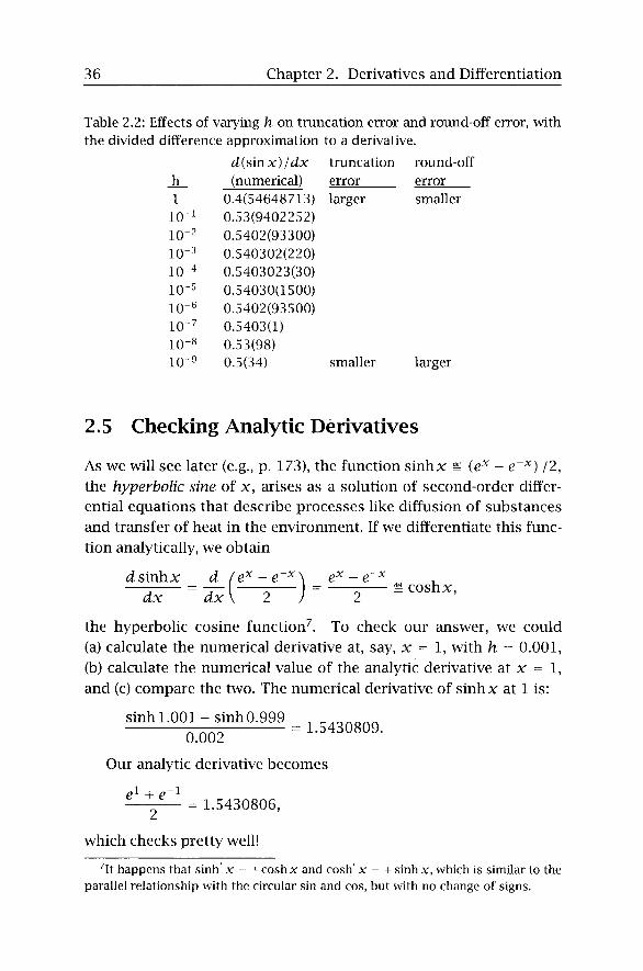
If we carry out similar calculations for various values of h, we find the results in Table 2.2, p. 36, which illustrate a compromise—as we go to smaller values of /x, the round-off error increases, and the so-called truncation error (caused by truncating the Taylor series at the quadratic term) decreases because we stay ever closer to the point of expansion. One of the exercises at the end of the chapter will help you to choose a reasonable h to use with your own calculator.


Table 2.2: Effects of varying h on truncation error and round-off error, with the divided difference approximation to a derivative.

J ]_ 1

10-1 10-2 10-3 10-^ 10-5 10-6 10-^ 10-8 10-9

^ ( s i n x ) / ^ x (numerical)

0.4(54648713) 0.53(9402252) 0.5402(93300) 0.540302(220) 0.5403023(30) 0.54030(1500) 0.5402(93500) 0.5403(1) 0.53(98) 0.5(34)

truncation error larger

smaller

round-off error smaller

larger

2.5 Checking Analytic Derivatives

As we will see later (e.g., p. 173), the function sinhx ^ (e^ - e~^) /2, the hyperbolic sine of x, arises as a solution of second-order differential equations that describe processes like diffusion of substances and transfer of heat in the environment. If we differentiate this function analytically, we obtain

(isinhx d (e^-e~^\ e^ + e~^

the hyperbolic cosine function''. To check our answer, we could (a) calculate the numerical derivative at, say, x = 1, with h = 0.001, (b) calculate the numerical value of the analytic derivative at x = 1, and (c) compare the two. The numerical derivative of sinhx at 1 is:

sinh 1.001-sinh 0.999 0.002

Our analytic derivative becomes

1.5430809.

e^ + e~^ = 1.5430806,

which checks pretty well!

''It happens that sinh' x = + coshx and cosh' x = + sinh x, which is similar to the parallel relationship with the circular sin and cos, but with no change of signs.

§2.6. Exercises 37

2.6 Exercises

Problem Set on Derivatives

1. Determine the derivative of the following function analytically, then find its numerical value when a = 2TT/12, b = 7, C = 0.01, g = 2, k = 3 and t = 3.

^ _ e~^^cos[a{t + b)]

2. Check your result to Exercise 1 using numerical differentiation, with the central difference of Eqn. 2.15, p. 34.

3. Calculate the actual (analytical) value of d(cosx)/dx at x == 2 and then check the result using

df ^ f{x + h)-f{x-h) dx ^ 2h

with h = I, 10"^, lO"'^, 10"^, and 10~^. Your goal is to determine a good h to use in your own calculator for similar calculations. When you locate the best value from those above, say 10"^, try ] Q-(N+i) ^ j ^^ iQ-{N-i) ^g ^gjj^ gQ yQ^ don't miss the best value.

4. Differentiate f(x) = x^ - x^-^ analytically, and then check the result numerically at the point x = 7. Be sure to show all steps of your work.

5. Use the chain rule to find dz/dx when y = sinbx and z = y^.

6. As manager of a large water quality research project, you have to design some special sample bottles, of which several thousand will be required. Each must:

• be cylindrical in shape

• have 1 liter capacity (1000 cm^)

• have the smallest internal surface area consistent with the other two criteria. This results from the need to line the bottles with a very costly non-reactive substance.

What should be the inside dimensions of the bottles, to satisfy these criteria?


7. You are setting up an experiment in a greenhouse. You need a seed bed surrounded by a plant-free border of 10 cm at the top and bottom, and 6 cm on each side. Space is limited, and you have been allocated a total of 2000 cm^ of area (seed bed plus border) on one of the tables. What overall dimensions should you choose to obtain the maximum area of seed bed? What will the actual seed bed area then be? (Note: the border is not part of the seed-bed area.)

As usual, try to solve this problem both symbohcally and numerically. Be sure to define any symbols you use.

8. Suppose it is found that the average annual concentration [ppm] of a pollutant at a "target point" at least 1 km away from a pollutant source is proportional to the average annual pollutant concentration at the source, divided by the distance between the source and the target point. The proportionality coefficient is some constant k [km]. Now consider a small city with two major sources of SO2. The average SO2 concentration at one is 110 ppm, and at the other is 230 ppm. The two sources are 7 km apart. If their effects at a target point are additive, and all other sources can be neglected, where along the line between the two sources (but at least 1 km from each) would the pollutant be a minimum?

9. Suppose the white oaks in a forest are a fraction / of the individual trees there, and that there are a total of Ut trees ha~^ (all species) in that stand. In other words, the stand contains / • Ut white oaks per hectare. Under that condition, the oaks produce m kg of acorns per tree per year, on average. Suppose that if the density of trees (stems per hectare) increased, the acorn production of each tree would decrease by 6 kg per tree per year per added tree [kg tree~^ yr~^ overall].

A. If only white oaks were added (and no stems of other species) what number of white oaks per hectare would produce the largest number of acorns per hectare per year? (The deer—weeds of the mammal world—who eat acorns, would like to know this.) For this part, provide that answer entirely in symbols.

B. If / = 40%, Ut = 120, m = 200, and 5 = 4, what number of white oaks would lead to maximum production of acorns, and what would that production be?

§2.6. Exercises 39

Hint: For a given density x of white oaks per hectare, acorn production p (you determine the units) is reduced from its original value, m, by an amount 5{x - fut).

10. The Ostrich Waste Disposal Corporation (OWDC) plans to build a landfill. They are constrained by state regulations to lay it out in trenches 10m wide, but they have some choice about trench depth. The trenches have vertical sides, and a horizontal bottom. They need a total trench volume of 30,000 m^.

The top covering for the trenches costs C dollars per square meter, and to reduce that cost, they would like to make the trenches deep. On the other hand, excavation costs increase quadratically with depth, and can be estimated as E = a -^ bZ^, where E is the excavation cost per unit length of 10-m wide trench [doUars/m], Z is trench depth [m], and a and b are constants.

A. What are the units of a and b?

B. What length and depth should the company choose to minimize its total construction costs for a landfill of the necessary size? Work this part entirely in symbols. Express your final answer in one (or a few) complete sentences.

11. The equation

I = a + i^sin — ( t + d)

is an approximate description of the daylength I between sunrise and sunset at 32 N latitude, as it varies with time of year t. (For data, see List 1949.) We'll work with 365-day years, and ignore leap years. The variables are:

L = daylength [minutes] a = annual average daylength [minutes] b = amplitude [minutes] c = period [days] d = "phase shift" [days], to make the peak fall near June 21.

We will define t = 0 at midnight between Dec. 31 and Jan. 1.

Sketch a graph of L versus t and work out the following:

• Differentiate the equation analytically (symbolically) to yield dL/dt.


• Using that derivative, calculate the numerical value of dL/dt at noon of January 1 (when t = 0.5 da) and at noon on September 21 (when t = 263.5 da). State the units and explain the physical meaning of these numbers. For these calculations, use a = 731.5, b = 170.5, c = 365, and d = -80.5.

• Check your derivative value for noon of January 1 by differentiating the original equation for I numerically at t = 0.5.

12. A forest ecologist estimates that the density D of acorns dropped near white oak trees decreases with distance x from the tree, with the relationship being D(x) = a/(l + x), where D is in acorns m~^ and X is in m. However, deer and squirrels are aware of this distribution—they learn that relationship in school—and thus forage most intensely near the trees. As a result, the probability P of any given acorn remaining on the ground and germinating increases with distance from the tree as given by P(x) = bx/{c + x). (That probability is also the fraction that germinates, on the average.)

Your tasks are to:

a) Determine the distance Xmax where the density of germinating acorns (in number m~ ) is greatest. Your answer should be given in terms of the symbohc constants, a, b, and c.

b) Explain how you know that you have found a maximum rather than a minimum.

c) If a = 3 acorns m~^ b = 0.5 m~^ and c = 40 m, then what is the numerical value of Xmax and of the maximum density of germinated acorns?

You'll likely find it helpful to sketch the two functions, and perhaps some combination of them as well.

Hint: Remember that a fraction can be zero either if the numerator is zero or if the denominator goes to infinity. In max-min problems, we are usually interested in solutions where the numerator goes to zero.

13. One afternoon while searching for spotted-owl nests, you use a topographic map and a GPS unit to keep careful track of where you are. At quitting time, you find yourself one mile east of the

§2.6. Exercises 41

north-south road on which you left your truck. Specifically, if you walked due west you would strike the road at a point three miles south of your truck.

You could walk the four miles along that right-angle path and you could walk straight toward your truck, as two limiting cases. However, you think you would get to your truck fastest if you angled through the woods to strike the road at a point that was less than three miles from the truck. You estimate that your walking speed through the woods would be two miles per hour, and your speed on the road would be four miles per hour.

a) To minimize your walking time, what point on the road (at what distance from your truck) should you aim for? For both parts of this problem, work in symbols for as long as you can, but then give numerical values.

b) What would your minimum walking time be, and how much time would you save compared with that along the right-angle path?

As always, you'll likely a sketch helpful.

Exercises on Taylor & Maclaurin Series

Reminder—In the field of analysis, one learns that "nice" functions (even transcendental ones^) can be expanded as Taylor series that are valid for all x within certain intervals. If a function/(x) is "expanded about" a point a, it takes the form described by Eqn. 2.10. Such a form can always be simplified to an infinite polynomial of the form

/ ( X ) = fco + i>\^ + ^2^^ + ^ 3 ^ ^ + • • •

and this fact is useful for doing approximate calculations in numerical analysis.

14. Show that:

• cos(-a) = cos(a). (Because of this, cos x is called an "even" function.)

A transcendental function is one that can't be expressed as a ratio of two polynomials. Examples are e^ and sinx.


• s in(-a) = - sin(+a). (sin x is an odd function.)

• e^^ = cosz + is inz, where i = ^ / ^ . To confirm this, it helps to work out first the values of i^, i^, i^, etc. You will find that an interesting pattern emerges.

15. The purpose of this exercise is to show that the Taylor series for a finite polynomial is that polynomial. E.g., consider

fix) = P^ix) = 7x^ - 3x, expanded about a = 4. (2.16)

We have: f{a) = 7(64) - 3(4) = 436, and from the rules for derivatives of positive powers (i.e., that dx^/dx = nx^~^)\

fix) = 2 1 x ^ - 3 , Sofia) = 2 1 ( 1 6 ) - 3 = 333,

fix) = 42x, so f'ia) = 42(4) = 168, and

r'ix)= 42, so r'ia)= 42.

Also, f^'^Hx) == 0 for all n > 3 and for all x. Substituting these into (1), we get the Taylor series:

1 68 fix) = 436 + 333(x - 4) + j^ji^ - 4)^ +

42 ( X - 4 ) ^ 0 + 0 + .... 3- 2- 1

Your jobs are to simplify this expression by grouping like powers of X, and to show that it reduces to the original polynomial (Eqn. 2.16).

16. Recalling that

dx

expand y = 1/x about the point a=2. Show the first 4 terms of the expansion. Use this truncated series to estimate / (2.1) , and compare the estimate with the true value of/(2.1) = 1/(2.1) obtained by division.

Note that the function fix) = 1/x is not a polynomial because it is not a sum of terms of positive powers of x. Hence, to be exact

§2.6. Exercises 43

the Taylor series for this function must have an infinite number of terms. Do you think your series would yield a reasonable approximation for / ( x ) at X = 0? Why or why not?

17. Expand y = R -\- Sx -\- Tx^ about x = a (symbolically), and show that the Taylor series expansion reduces to the original polynomial.

18. Given: The derivative of y = e^^ is be^^, and (as you may remember) for any function y and any constant c,

d{cy) _ dy dx dx'

Using these facts, expand y = ce^^ as a Maclaurin series (which means you set a = 0). Then show that that series reduces to c times e^ when u = bx. For this, you can take as given that for any u,

,. ^ u^ u^ u^

19. Expand f{x) = xe^ about a = 1 through the [x -1]^ (third-order) term. What are the relative errors that result if you use this truncated Taylor series to estimate/(1.1), / (1.2) , / (1 .4) , / ( 1 . 8 ) , / ( 2 . 6 ) , / ( 4 . 2 ) and / (7 .4 ) ?

20. Expand the function fix) = log(x) as a Taylor series around the point a= 1, keeping terms up to and including the term based on the third derivative.

What approximate value does your series provide for log(l.l)? Then, if you assume that your calculator yields the exact true value for that quantity, what is the relative error of the approximate value calculated from your series?

21. The net exchange R of long-wave (thermal) radiation between an object (such as a leaf or an animal) and its surroundings is given by R(T) = aeiT"^ - Tf), where a is the Stefan-Boltzmann constant [J cm~^ s~^ deg"'*], e is the emissivity (or "blackness") of the object in far-infrared wavelengths [unitless], T is the object's absolute


surface temperature [deg K], and Ts is the absolute temperature of surrounding objects. R is one term of the energy balance of an object. Assuming that Ts is a known constant, determine the first five terms of the Taylor series for R{T), expanded about the temperature T = a.

22. This problem makes use of the Maclaurin series for e^, which as you have seen is

6^ = l + x + ^ + ^ + . - . . (2.17)

In risk assessment for carcinogens, test animals like rats are often fed high doses of a chemical. Then assessors use a mathematical model to estimate the mean number ju of tumors per animal expected to occur in rats fed some lower dose to which humans might be exposed. From JL/, the assessors wish to estimate the carcinogenic potency (p, which is defined as the probabihty that a rat fed that lower dose would get cancer; i.e., one or more tumors.

At the low doses considered, cancers are rare, and so the Poisson distribution from statistics can be used to show that the probability of a given rat's not getting cancer is P(0) = e~^. Thus the probability that a rat will suffer from one or more tumors is <p = l-P{0) = l - e~^, and this is the quantity we seek. Suppose for a particular dose of a particular chemical that n is quite small, say 0.0001. Then use the series in Eqn. 2.17 to show that for all practical purposes, <p = ju. Describe your logic. (Ultimately the potency for rats is converted to a potency for humans, but that's another story.)

23. (This problem is about integration, but does not require you to perform any integration.) As noted on p. 44, the equation for the "bell curve" of statistics; i.e., for the standard normal distribution, is

p(z) = - ^ e x p f - y V (2.18)

Unfortunately that analytic expression is not directly useful much of the time because it yields the probability density at any value of z, and not the actual probabihties that we usually want to work

§2.6. Exercises 45

with. To calculate the probability P that a standard normal random variable Z lies in some range of interest, we have to integrate p(z) over that range. Sadly, p{z) can't be integrated analytically.

Suppose we needed P(0 < z < 0.8) for some statistical application. One way to obtain that value would be to write the Taylor series for p{z) (expanded about a = 0.4, say), to truncate that series after k terms, and to sum the integrals of those terms. If we kept enough terms, that should work reasonably well, since the integral of a sum is the sum of the integrals.

Although you need not perform any integration, your task here is to check out how well a few terms of the Taylor series for p{z) approximate that function. In particular,

A. Find the first three terms (i.e., through the quadratic term) of the Taylor series for p(z), expanded about 0.4.

B. Calculate the true numerical value of p{0) and of p(0.8) from Eqn. 2.18, to as many digits as your calculator supplies.

C. Calculate the approximate value of p(0) that would be obtained from the three terms of the Taylor series, and determine the relative error of that approximation.

D. Repeat the calculations from Part C at z = 0.8.

If those errors are relatively small, that would suggest (but not prove) that the integral of the three-term series would approximate the integral of the true p{z) reasonably well over this range. If not, you might want to add more terms, but as the higher derivatives get messy, we'll omit that here.

Hints: To simphfy developing the Taylor series, you may find it helpful to give the leading constant in the formula for p{z) a symbolic name (like c); use a substitution like giz) = - z^ /2 , and make use of the chain rule.

24. At X = 3, a certain function has the value / ( 3 ) = 1, and its first three derivatives there have the values f = 1/2, f = 1/4, and /^^^ = 1/8. The fourth and all higher derivatives are zero at x = 3. Using this information and the properties of Taylor series, write a formula that would allow an assistant to calculate values of fix) for any value of x.


25. In energy-balance calculations similar to the one for the top of a car on p. 8, a quantity like q(T) = (T"^ - A^) frequently arises, and analysts often "linearize" that with the help of Taylor series to simplify solving for temperature. Find the first three terms of the Taylor series for the function (^(T) expanded around the point T = A] i.e., the constant term and those involving (T - A) and {T - A)^. Then, calculate the numerical values of each of those three terms if T == 300° K and A = 295° K. Linearization involves dropping the third (and higher) terms. How large is that third term, relative to the sum of the first two, in this application? Can it reasonably be dropped?

2.7 Questions and Answers

1. Please explain again why the derivative of y = fix) = e^^ is fix) = he^''.

• This is a good place to use the chain rule. Define u = bx. Then y = giu) = e^y and u = hix) = bx. The chain rule says that dy/dx = idyIdu)iduIdx) = ie^)(b). Now replace the u with bx, and you have dy/dx = ie^^)ib) = be^^. Alternatively, you can work with the Maclaurin series for e^\ i.e., with

,, , u^ u^ li^ . - = l + u + — + — + — + . . . .

Now substitute u = bx, and then differentiate the result term by term. Remember that the derivative of a sum is the sum of the derivatives. You should be able to factor out a b from the result, and what's left will be expibx)/b = exp(u).

2. Is there a table of derivatives and integrals we can use for reference?

• There are lots available. The firm that publishes the Handbook of Chemistry and Physics extracts the math tables from that book as a smaller book, and you can buy that. The Handbook of Mathematical Functions is a fine reference book by Abramowitz and Stegun, originally pubhshed by the National Bureau of Standards (Now the National Institute of Standards & Technology), and later, in paperback, by Dover—it's a big tome, however. Some of the "outline

§2.7. Questions and Answers 47

series" of books (e.g., Schaum's) have tables available, I think. I've seen other books of tables in various bookstores, and any of them ought to be helpful.

3. Fm unsure of when you use [f{a + h) - f{a)]/h and when you just differentiate analytically.

• You should differentiate analytically most of the time—it's more exact. But you can use the finite difference form (A) to check analytic derivatives, (B) when you have only a list of values of the function, not the function itself, and (C)—yet to come—as the basis for approximate solutions to differential equations. Remember that the central difference form [/(a + h) - f{a - h)]/{2h) is almost always preferable to the forward difference you asked about.

4. Please give another example of the chain rule.

• That would also be a good thing to look up in a calculus text for a good general description. For an example, though, suppose the water temperature in some lake varied with time on summer days as r = a + f? sin(ct), and suppose evaporation rate from the water depended on temperature according to E = a • exp(fcr). Then ultimately E would vary with time through this "chain" of dependencies. Thus, to see how rapidly E would change with time at some particular time, you could use dE/dt = {dE/dT){dT/dt), which is the chain rule. Here dE/dT = akexpikT), and dT/dt = bccosict).

5. Why again is the derivative of log{bx) equal to 1/x?

• logbx = logb -\- logx (log of a product is the sum of the logs). \ogb is a constant, so its derivative is zero. Thus, d(logbx)/dx = 0 + d(logx)/dx = 1/x. That one seems counterintuitive at first, doesn't it?

6. When you gave the rule that d{u + w) /dx = du/dx + dw /dx, why did you specify that u = f{x) and w = g{x)7

• It only makes sense to differentiate u with respect to x if tt is a function of x. The 'u = / ( x ) ' was just meant to tell you that it is.

7. What are the apphcations of Taylor series?

• They are often used as the basis for approximations.


They form the basis for much of numerical analysis. (This is related to the first point.) We will use them at various times in the semester either to derive numerical methods (e.g., Newton's method for finding roots of non-linear equations) or to justify and help understand the behavior of other methods.

They are used a great deal by mathematical modellers, engineers, and other applied mathematicians. For those of you whose goal in the course is to be able to work with such people, a basic understanding of Taylor series (and that's our level—very basic) should help you communicate with them.

A side benefit in working with Taylor series is that you get some useful practice differentiating.

8. How can you get so much information from a Taylor series, when all you know about is one point?

• Well, you have to know a lot about that one point! You'll see as we get further into it (the short distance farther that we will go) that the first N terms of a Taylor series are equivalent to a polynomial of order AT - 1. That means that knowing the function and N derivatives at a single point tells you quite a lot about how the function curves and varies, at least in the near neighborhood of that point.

If you know the y value at a given x, and you know the slope, you can move left or right a short distance on the tangent line, and be close to the value of the function there. If you know both the first and second derivatives there, that gives you an estimate of how much you should correct for curvature. Each additional derivative helps you to correct more and more.

9. In a Taylor series, what are a and x, and especially, what is the difference?

• X is the general variable (on the x axis), while a is the specific value of X about which we "expand the function." That is, a is the X value for which we must know the value of the function and its derivatives. If we truncate the series at a finite number of terms, then the resulting approximation will generally be better when x is near a than when x is far from a.


10. If we can obtain square roots from our calculators, or if we already know some other / (x ) , why do we need Taylor series?

• The square root example illustrated what a Taylor series is, the steps you have to go through to get one, and the fact that these series yield better approximations near a (i.e., in a narrow range around the point of expansion), and better approximations with more terms (at least near a).

If you go on a long research trip some time, and drop your calculator in a lake, you now know one way to get the square root of 5 <grin>. That's not too far fetched, I guess. You might have to triangulate withx^ + y^ = z^ (fromwhichz = Jx^ -i- y^\to find locations on a lake, or some such thing.

More reahstically, If your calculator doesn't give hyperbolic sines and cosines, you now have a way to get those. That is, Taylor series are used for many other kinds of functions in addition to square roots.

Most important, we now have a justification for using polynomials to approximate general (non-polynomial) functions, and we know that these approximations work better in narrow ranges and with more terms. This is the major reason we deal here with Taylor series—they form the basis for most numerical methods.

11. Does the second derivative show how the slope is changing? For example, does a negative second derivative tell you that the slope is getting less steep as x increases?

• Yes, and yes. The second derivative is just the slope of the slope (It tells you how fast the slope changes with increasing x). A negative / ' ' tells you that f gets smaller as x increases.

When you do a max-min problem, you find a point where the first derivative is zero. To determine whether that is a maximum or a minimum point, you can calculate the second derivative at that point. If / ' ' is positive there, it means that the slope keeps getting bigger as you move to the right. Therefore, the function is cupped upward, and you have a minimum. If f is negative at your extreme point, then the slope keeps getting smaller as you move to the right. That means that the function is cupped downward at the extremum, so the point is a maximum. See any calculus book


if you want more on this. Also, try some sketches to see it better.

Conceptually, this indicates why including a second-derivative term {f"{x - a)^/2\) improves a Taylor series. The information about how the slope changes as you move away from x = a helps to predict fix), relative to what you would get from using just f{a) and f'(a) (the starting value and the starting slope).

12. How is a Taylor series different from linear approximation, where fix) ~ fia) + f'ia)Ax7 Is the Taylor series more exact?

• One way to look at this is that a linear approximation is the simplest form of approximation based on the Taylor series—it is equivalent to using the first two terms of a Taylor series. The Taylor series is more exact if you keep more terms, but if you drop all but the first two terms, the two are identical. Linear approximations are very common, but during the semester we will use some quadratic ones (like the central difference derivative) and one quartic (fourth-order) one. Stay tuned.

13. What does your example on p. 35 have to do with Taylor series? What do those calculations illustrate?

• Those calculations are in the "numerical differentiation" section. They are indirectly related to Taylor series in the sense that Taylor series tell us it is better to use central differences than to use forward differences. But these calculations illustrate a completely different point, namely that if you use too small an "h" value (that would be good from the point of view of Taylor series, which tell us to work in a very small range), then the new problem of roundoff error rears its ugly head. There are tradeoffs like this in a lot of numerical work. Keeping ranges small helps from one point of view, but often increases round-off error. Applied math (like life) is full of compromises.

14. Shouldn't there be a 'remainder term' at the end of a Taylor series?

• If you truncate a Taylor series (i.e., cut it off after a finite number of terms) then it would often have a remainder term added to it, as you have evidently seen elsewhere. However, so far I think the series I've written have all had a "+..." at the end, indicating a (theoretically) infinite series of terms. The full series does not have a remainder. Also, Taylor series for polynomials can be exact with


a finite number of terms, and they don't need remainder terms either.

15. What is the meaning of second and higher derivatives, hke / ' ' ( x ) , f'"{x), and so on?

• That would be a good thing to review in an introductory calculus text, but let me explain it too. Take the function y = fix) = x^ + 3x, say. Wherever you go on the x axis, the slope of the curve above that point (the "rise" over the "run") can be calculated using the first derivative, which is fix) = Sx"^ + 3. You can treat that derivative as a function too. If you do, and take its derivative everywhere, you would get "derivative of 5x^^+3'' = 20x^ + 0 = 20x^. That new function is just the second derivative of the original function. It tells you how fast the slope of the original function changes as you move from one value of x to another. A 20th derivative is just the derivative with respect to x of the 19th derivative (etc.). (For fix) = x^ + 3x, every derivative above the fifth would be zero, however.)

16. What is the point of working with a Taylor series if you just get the original function back?

• That happens only if your original function is a polynomial. It didn't happen with the square-root example we've started to work with, as you saw. Finding the Taylor series for a polynomial is instructional, though, because it shows the close relationship between those two mathematical forms.

17. With a Taylor series, do you always need an infinite number of terms, or can you stop once the terms become zero?

• (Infinity) x (zero) is still zero, so if you know that all remaining possible terms are zero, then you can stop because you know that adding them won't make any difference. Generally that happens only with polynomials, however.

derivatives and differentiation

Documents