derivations of applied mathematics - · pdf file1.1 applied mathematics . . . . . . . . . . ....
TRANSCRIPT

Derivations of Applied Mathematics
Thaddeus H. Black
Revised 27 March 2007

ii
Thaddeus H. Black, 1967–.Derivations of Applied Mathematics.27 March 2007.U.S. Library of Congress class QA401.
Copyright c© 1983–2007 by Thaddeus H. Black 〈[email protected]〉.
Published by the Debian Project [10].
This book is free software. You can redistribute and/or modify it under theterms of the GNU General Public License [16], version 2.

Contents
Preface xv
1 Introduction 1
1.1 Applied mathematics . . . . . . . . . . . . . . . . . . . . . . . 1
1.2 Rigor . . . . . . . . . . . . . . . . . . . . . . . . . . . . . . . . 2
1.2.1 Axiom and definition . . . . . . . . . . . . . . . . . . . 2
1.2.2 Mathematical extension . . . . . . . . . . . . . . . . . 4
1.3 Complex numbers and complex variables . . . . . . . . . . . . 5
1.4 On the text . . . . . . . . . . . . . . . . . . . . . . . . . . . . 5
2 Classical algebra and geometry 7
2.1 Basic arithmetic relationships . . . . . . . . . . . . . . . . . . 7
2.1.1 Commutivity, associativity, distributivity . . . . . . . 7
2.1.2 Negative numbers . . . . . . . . . . . . . . . . . . . . 9
2.1.3 Inequality . . . . . . . . . . . . . . . . . . . . . . . . . 10
2.1.4 The change of variable . . . . . . . . . . . . . . . . . . 11
2.2 Quadratics . . . . . . . . . . . . . . . . . . . . . . . . . . . . 11
2.3 Notation for series sums and products . . . . . . . . . . . . . 13
2.4 The arithmetic series . . . . . . . . . . . . . . . . . . . . . . . 15
2.5 Powers and roots . . . . . . . . . . . . . . . . . . . . . . . . . 15
2.5.1 Notation and integral powers . . . . . . . . . . . . . . 16
2.5.2 Roots . . . . . . . . . . . . . . . . . . . . . . . . . . . 17
2.5.3 Powers of products and powers of powers . . . . . . . 19
2.5.4 Sums of powers . . . . . . . . . . . . . . . . . . . . . . 20
2.5.5 Summary and remarks . . . . . . . . . . . . . . . . . . 20
2.6 Multiplying and dividing power series . . . . . . . . . . . . . 21
2.6.1 Multiplying power series . . . . . . . . . . . . . . . . . 22
2.6.2 Dividing power series . . . . . . . . . . . . . . . . . . 22
2.6.3 Dividing power series by matching coefficients . . . . . 26
iii

iv CONTENTS
2.6.4 Common quotients and the geometric series . . . . . . 29
2.6.5 Variations on the geometric series . . . . . . . . . . . 29
2.7 Constants and variables . . . . . . . . . . . . . . . . . . . . . 30
2.8 Exponentials and logarithms . . . . . . . . . . . . . . . . . . 32
2.8.1 The logarithm . . . . . . . . . . . . . . . . . . . . . . 32
2.8.2 Properties of the logarithm . . . . . . . . . . . . . . . 33
2.9 Triangles and other polygons: simple facts . . . . . . . . . . . 33
2.9.1 Triangle area . . . . . . . . . . . . . . . . . . . . . . . 34
2.9.2 The triangle inequalities . . . . . . . . . . . . . . . . . 34
2.9.3 The sum of interior angles . . . . . . . . . . . . . . . . 35
2.10 The Pythagorean theorem . . . . . . . . . . . . . . . . . . . . 36
2.11 Functions . . . . . . . . . . . . . . . . . . . . . . . . . . . . . 38
2.12 Complex numbers (introduction) . . . . . . . . . . . . . . . . 39
2.12.1 Rectangular complex multiplication . . . . . . . . . . 41
2.12.2 Complex conjugation . . . . . . . . . . . . . . . . . . . 41
2.12.3 Power series and analytic functions (preview) . . . . . 43
3 Trigonometry 45
3.1 Definitions . . . . . . . . . . . . . . . . . . . . . . . . . . . . . 45
3.2 Simple properties . . . . . . . . . . . . . . . . . . . . . . . . . 47
3.3 Scalars, vectors, and vector notation . . . . . . . . . . . . . . 47
3.4 Rotation . . . . . . . . . . . . . . . . . . . . . . . . . . . . . . 51
3.5 Trigonometric sums and differences . . . . . . . . . . . . . . . 53
3.5.1 Variations on the sums and differences . . . . . . . . . 54
3.5.2 Trigonometric functions of double and half angles . . . 55
3.6 Trigonometrics of the hour angles . . . . . . . . . . . . . . . . 55
3.7 The laws of sines and cosines . . . . . . . . . . . . . . . . . . 59
3.8 Summary of properties . . . . . . . . . . . . . . . . . . . . . . 60
3.9 Cylindrical and spherical coordinates . . . . . . . . . . . . . . 62
3.10 The complex triangle inequalities . . . . . . . . . . . . . . . . 64
3.11 De Moivre’s theorem . . . . . . . . . . . . . . . . . . . . . . . 65
4 The derivative 67
4.1 Infinitesimals and limits . . . . . . . . . . . . . . . . . . . . . 67
4.1.1 The infinitesimal . . . . . . . . . . . . . . . . . . . . . 68
4.1.2 Limits . . . . . . . . . . . . . . . . . . . . . . . . . . . 69
4.2 Combinatorics . . . . . . . . . . . . . . . . . . . . . . . . . . 70
4.2.1 Combinations and permutations . . . . . . . . . . . . 70
4.2.2 Pascal’s triangle . . . . . . . . . . . . . . . . . . . . . 72
4.3 The binomial theorem . . . . . . . . . . . . . . . . . . . . . . 72

CONTENTS v
4.3.1 Expanding the binomial . . . . . . . . . . . . . . . . . 72
4.3.2 Powers of numbers near unity . . . . . . . . . . . . . . 73
4.3.3 Complex powers of numbers near unity . . . . . . . . 74
4.4 The derivative . . . . . . . . . . . . . . . . . . . . . . . . . . . 75
4.4.1 The derivative of the power series . . . . . . . . . . . . 75
4.4.2 The Leibnitz notation . . . . . . . . . . . . . . . . . . 76
4.4.3 The derivative of a function of a complex variable . . 78
4.4.4 The derivative of za . . . . . . . . . . . . . . . . . . . 79
4.4.5 The logarithmic derivative . . . . . . . . . . . . . . . . 79
4.5 Basic manipulation of the derivative . . . . . . . . . . . . . . 80
4.5.1 The derivative chain rule . . . . . . . . . . . . . . . . 80
4.5.2 The derivative product rule . . . . . . . . . . . . . . . 81
4.6 Extrema and higher derivatives . . . . . . . . . . . . . . . . . 82
4.7 L’Hopital’s rule . . . . . . . . . . . . . . . . . . . . . . . . . . 84
4.8 The Newton-Raphson iteration . . . . . . . . . . . . . . . . . 85
5 The complex exponential 89
5.1 The real exponential . . . . . . . . . . . . . . . . . . . . . . . 89
5.2 The natural logarithm . . . . . . . . . . . . . . . . . . . . . . 92
5.3 Fast and slow functions . . . . . . . . . . . . . . . . . . . . . 94
5.4 Euler’s formula . . . . . . . . . . . . . . . . . . . . . . . . . . 96
5.5 Complex exponentials and de Moivre . . . . . . . . . . . . . . 99
5.6 Complex trigonometrics . . . . . . . . . . . . . . . . . . . . . 99
5.7 Summary of properties . . . . . . . . . . . . . . . . . . . . . . 101
5.8 Derivatives of complex exponentials . . . . . . . . . . . . . . 101
5.8.1 Derivatives of sine and cosine . . . . . . . . . . . . . . 101
5.8.2 Derivatives of the trigonometrics . . . . . . . . . . . . 103
5.8.3 Derivatives of the inverse trigonometrics . . . . . . . . 105
5.9 The actuality of complex quantities . . . . . . . . . . . . . . . 106
6 Primes, roots and averages 109
6.1 Prime numbers . . . . . . . . . . . . . . . . . . . . . . . . . . 109
6.1.1 The infinite supply of primes . . . . . . . . . . . . . . 109
6.1.2 Compositional uniqueness . . . . . . . . . . . . . . . . 110
6.1.3 Rational and irrational numbers . . . . . . . . . . . . 113
6.2 The existence and number of roots . . . . . . . . . . . . . . . 114
6.2.1 Polynomial roots . . . . . . . . . . . . . . . . . . . . . 114
6.2.2 The fundamental theorem of algebra . . . . . . . . . . 115
6.3 Addition and averages . . . . . . . . . . . . . . . . . . . . . . 116
6.3.1 Serial and parallel addition . . . . . . . . . . . . . . . 116

vi CONTENTS
6.3.2 Averages . . . . . . . . . . . . . . . . . . . . . . . . . 119
7 The integral 123
7.1 The concept of the integral . . . . . . . . . . . . . . . . . . . 123
7.1.1 An introductory example . . . . . . . . . . . . . . . . 124
7.1.2 Generalizing the introductory example . . . . . . . . . 127
7.1.3 The balanced definition and the trapezoid rule . . . . 127
7.2 The antiderivative . . . . . . . . . . . . . . . . . . . . . . . . 128
7.3 Operators, linearity and multiple integrals . . . . . . . . . . . 130
7.3.1 Operators . . . . . . . . . . . . . . . . . . . . . . . . . 130
7.3.2 A formalism . . . . . . . . . . . . . . . . . . . . . . . . 131
7.3.3 Linearity . . . . . . . . . . . . . . . . . . . . . . . . . 132
7.3.4 Summational and integrodifferential transitivity . . . . 133
7.3.5 Multiple integrals . . . . . . . . . . . . . . . . . . . . . 135
7.4 Areas and volumes . . . . . . . . . . . . . . . . . . . . . . . . 137
7.4.1 The area of a circle . . . . . . . . . . . . . . . . . . . . 137
7.4.2 The volume of a cone . . . . . . . . . . . . . . . . . . 137
7.4.3 The surface area and volume of a sphere . . . . . . . . 138
7.5 Checking an integration . . . . . . . . . . . . . . . . . . . . . 141
7.6 Contour integration . . . . . . . . . . . . . . . . . . . . . . . 142
7.7 Discontinuities . . . . . . . . . . . . . . . . . . . . . . . . . . 143
7.8 Remarks (and exercises) . . . . . . . . . . . . . . . . . . . . . 146
8 The Taylor series 149
8.1 The power series expansion of 1/(1 − z)n+1 . . . . . . . . . . 150
8.1.1 The formula . . . . . . . . . . . . . . . . . . . . . . . . 150
8.1.2 The proof by induction . . . . . . . . . . . . . . . . . 152
8.1.3 Convergence . . . . . . . . . . . . . . . . . . . . . . . 153
8.1.4 General remarks on mathematical induction . . . . . . 154
8.2 Shifting a power series’ expansion point . . . . . . . . . . . . 155
8.3 Expanding functions in Taylor series . . . . . . . . . . . . . . 157
8.4 Analytic continuation . . . . . . . . . . . . . . . . . . . . . . 159
8.5 Branch points . . . . . . . . . . . . . . . . . . . . . . . . . . . 161
8.6 Entire and meromorphic functions . . . . . . . . . . . . . . . 162
8.7 Cauchy’s integral formula . . . . . . . . . . . . . . . . . . . . 163
8.7.1 The meaning of the symbol dz . . . . . . . . . . . . . 164
8.7.2 Integrating along the contour . . . . . . . . . . . . . . 165
8.7.3 The formula . . . . . . . . . . . . . . . . . . . . . . . . 168
8.7.4 Enclosing a multiple pole . . . . . . . . . . . . . . . . 169
8.8 Taylor series for specific functions . . . . . . . . . . . . . . . . 170

CONTENTS vii
8.9 Error bounds . . . . . . . . . . . . . . . . . . . . . . . . . . . 171
8.9.1 Examples . . . . . . . . . . . . . . . . . . . . . . . . . 171
8.9.2 Majorization . . . . . . . . . . . . . . . . . . . . . . . 174
8.9.3 Geometric majorization . . . . . . . . . . . . . . . . . 175
8.9.4 Calculation outside the fast convergence domain . . . 177
8.9.5 Nonconvergent series . . . . . . . . . . . . . . . . . . . 178
8.9.6 Remarks . . . . . . . . . . . . . . . . . . . . . . . . . . 178
8.10 Calculating 2π . . . . . . . . . . . . . . . . . . . . . . . . . . 179
8.11 Odd and even functions . . . . . . . . . . . . . . . . . . . . . 180
8.12 Trigonometric poles . . . . . . . . . . . . . . . . . . . . . . . 180
8.13 The Laurent series . . . . . . . . . . . . . . . . . . . . . . . . 182
8.14 Taylor series in 1/z . . . . . . . . . . . . . . . . . . . . . . . . 184
8.15 The multidimensional Taylor series . . . . . . . . . . . . . . . 186
9 Integration techniques 189
9.1 Integration by antiderivative . . . . . . . . . . . . . . . . . . . 189
9.2 Integration by substitution . . . . . . . . . . . . . . . . . . . 190
9.3 Integration by parts . . . . . . . . . . . . . . . . . . . . . . . 191
9.4 Integration by unknown coefficients . . . . . . . . . . . . . . . 193
9.5 Integration by closed contour . . . . . . . . . . . . . . . . . . 196
9.6 Integration by partial-fraction expansion . . . . . . . . . . . . 200
9.6.1 Partial-fraction expansion . . . . . . . . . . . . . . . . 200
9.6.2 Multiple poles . . . . . . . . . . . . . . . . . . . . . . 201
9.6.3 Integrating rational functions . . . . . . . . . . . . . . 204
9.6.4 Multiple poles (the conventional technique) . . . . . . 206
9.7 Frullani’s integral . . . . . . . . . . . . . . . . . . . . . . . . . 208
9.8 Products of exponentials, powers and logs . . . . . . . . . . . 210
9.9 Integration by Taylor series . . . . . . . . . . . . . . . . . . . 211
10 Cubics and quartics 213
10.1 Vieta’s transform . . . . . . . . . . . . . . . . . . . . . . . . . 214
10.2 Cubics . . . . . . . . . . . . . . . . . . . . . . . . . . . . . . . 214
10.3 Superfluous roots . . . . . . . . . . . . . . . . . . . . . . . . . 217
10.4 Edge cases . . . . . . . . . . . . . . . . . . . . . . . . . . . . . 219
10.5 Quartics . . . . . . . . . . . . . . . . . . . . . . . . . . . . . . 221
10.6 Guessing the roots . . . . . . . . . . . . . . . . . . . . . . . . 223
11 The matrix 227
11.1 Provenance and basic use . . . . . . . . . . . . . . . . . . . . 230
11.1.1 The linear transformation . . . . . . . . . . . . . . . . 230

viii CONTENTS
11.1.2 Matrix multiplication (and addition) . . . . . . . . . . 231
11.1.3 Row and column operators . . . . . . . . . . . . . . . 23311.1.4 The transpose and the adjoint . . . . . . . . . . . . . 234
11.2 The Kronecker delta . . . . . . . . . . . . . . . . . . . . . . . 23511.3 Dimensionality and matrix forms . . . . . . . . . . . . . . . . 236
11.3.1 The null and dimension-limited matrices . . . . . . . . 23811.3.2 The identity, scalar and extended matrices . . . . . . . 239
11.3.3 The active region . . . . . . . . . . . . . . . . . . . . . 24111.3.4 Other matrix forms . . . . . . . . . . . . . . . . . . . 241
11.3.5 The rank-r identity matrix . . . . . . . . . . . . . . . 24211.3.6 The truncation operator . . . . . . . . . . . . . . . . . 24311.3.7 The elementary vector and lone-element matrix . . . . 243
11.3.8 Off-diagonal entries . . . . . . . . . . . . . . . . . . . 24411.4 The elementary operator . . . . . . . . . . . . . . . . . . . . . 244
11.4.1 Properties . . . . . . . . . . . . . . . . . . . . . . . . . 24611.4.2 Commutation and sorting . . . . . . . . . . . . . . . . 247
11.5 Inversion and similarity (introduction) . . . . . . . . . . . . . 24811.6 Parity . . . . . . . . . . . . . . . . . . . . . . . . . . . . . . . 252
11.7 The quasielementary operator . . . . . . . . . . . . . . . . . . 25411.7.1 The general interchange operator . . . . . . . . . . . . 255
11.7.2 The general scaling operator . . . . . . . . . . . . . . 25611.7.3 Addition quasielementaries . . . . . . . . . . . . . . . 257
11.8 The triangular matrix . . . . . . . . . . . . . . . . . . . . . . 25911.8.1 Construction . . . . . . . . . . . . . . . . . . . . . . . 260
11.8.2 The product of like triangular matrices . . . . . . . . 26111.8.3 Inversion . . . . . . . . . . . . . . . . . . . . . . . . . 262
11.8.4 The parallel triangular matrix . . . . . . . . . . . . . . 26311.8.5 The partial triangular matrix . . . . . . . . . . . . . . 266
11.9 The shift operator . . . . . . . . . . . . . . . . . . . . . . . . 267
12 Rank and the Gauss-Jordan 269
12.1 Linear independence . . . . . . . . . . . . . . . . . . . . . . . 27012.2 The elementary similarity transformation . . . . . . . . . . . 272
12.3 The Gauss-Jordan factorization . . . . . . . . . . . . . . . . . 27212.3.1 Motive . . . . . . . . . . . . . . . . . . . . . . . . . . . 274
12.3.2 Method . . . . . . . . . . . . . . . . . . . . . . . . . . 27612.3.3 The algorithm . . . . . . . . . . . . . . . . . . . . . . 277
12.3.4 Rank and independent rows . . . . . . . . . . . . . . . 28512.3.5 Inverting the factors . . . . . . . . . . . . . . . . . . . 286
12.3.6 Truncating the factors . . . . . . . . . . . . . . . . . . 287

CONTENTS ix
12.3.7 Marginalizing the factor In . . . . . . . . . . . . . . . 28812.4 Vector replacement . . . . . . . . . . . . . . . . . . . . . . . . 28912.5 Rank . . . . . . . . . . . . . . . . . . . . . . . . . . . . . . . . 292
12.5.1 A logical maneuver . . . . . . . . . . . . . . . . . . . . 29312.5.2 The impossibility of identity-matrix promotion . . . . 29412.5.3 General matrix rank and its uniqueness . . . . . . . . 29712.5.4 The full-rank matrix . . . . . . . . . . . . . . . . . . . 29912.5.5 The full-rank factorization . . . . . . . . . . . . . . . . 30012.5.6 The significance of rank uniqueness . . . . . . . . . . . 300
13 Inversion and eigenvalue 30313.1 Inverting the square matrix . . . . . . . . . . . . . . . . . . . 30313.2 The exactly determined linear system . . . . . . . . . . . . . 30513.3 The determinant . . . . . . . . . . . . . . . . . . . . . . . . . 306
13.3.1 Basic properties . . . . . . . . . . . . . . . . . . . . . 30713.3.2 The determinant and the elementary operator . . . . . 31013.3.3 The determinant of the singular matrix . . . . . . . . 31113.3.4 The determinant of a matrix product . . . . . . . . . 31213.3.5 Inverting the square matrix by determinant . . . . . . 313
13.4 Coincident properties . . . . . . . . . . . . . . . . . . . . . . . 31413.5 The eigenvalue . . . . . . . . . . . . . . . . . . . . . . . . . . 31513.6 The eigenvector . . . . . . . . . . . . . . . . . . . . . . . . . . 31613.7 The dot product . . . . . . . . . . . . . . . . . . . . . . . . . 32013.8 Orthonormalization . . . . . . . . . . . . . . . . . . . . . . . . 321
14 Matrix algebra (to be written) 325
A Hex and other notational matters 329A.1 Hexadecimal numerals . . . . . . . . . . . . . . . . . . . . . . 330A.2 Avoiding notational clutter . . . . . . . . . . . . . . . . . . . 331
B The Greek alphabet 333
C Manuscript history 337

x CONTENTS

List of Figures
1.1 Two triangles. . . . . . . . . . . . . . . . . . . . . . . . . . . . 4
2.1 Multiplicative commutivity. . . . . . . . . . . . . . . . . . . . 8
2.2 The sum of a triangle’s inner angles: turning at the corner. . 35
2.3 A right triangle. . . . . . . . . . . . . . . . . . . . . . . . . . 37
2.4 The Pythagorean theorem. . . . . . . . . . . . . . . . . . . . 37
2.5 The complex (or Argand) plane. . . . . . . . . . . . . . . . . 40
3.1 The sine and the cosine. . . . . . . . . . . . . . . . . . . . . . 46
3.2 The sine function. . . . . . . . . . . . . . . . . . . . . . . . . 47
3.3 A two-dimensional vector u = xx+ yy. . . . . . . . . . . . . 49
3.4 A three-dimensional vector v = xx+ yy + zz. . . . . . . . . . 49
3.5 Vector basis rotation. . . . . . . . . . . . . . . . . . . . . . . . 52
3.6 The 0x18 hours in a circle. . . . . . . . . . . . . . . . . . . . . 57
3.7 Calculating the hour trigonometrics. . . . . . . . . . . . . . . 57
3.8 The laws of sines and cosines. . . . . . . . . . . . . . . . . . . 59
3.9 A point on a sphere. . . . . . . . . . . . . . . . . . . . . . . . 63
4.1 The plan for Pascal’s triangle. . . . . . . . . . . . . . . . . . . 72
4.2 Pascal’s triangle. . . . . . . . . . . . . . . . . . . . . . . . . . 73
4.3 A local extremum. . . . . . . . . . . . . . . . . . . . . . . . . 83
4.4 A level inflection. . . . . . . . . . . . . . . . . . . . . . . . . . 84
4.5 The Newton-Raphson iteration. . . . . . . . . . . . . . . . . . 86
5.1 The natural exponential. . . . . . . . . . . . . . . . . . . . . . 92
5.2 The natural logarithm. . . . . . . . . . . . . . . . . . . . . . . 93
5.3 The complex exponential and Euler’s formula. . . . . . . . . . 97
5.4 The derivatives of the sine and cosine functions. . . . . . . . . 103
7.1 Areas representing discrete sums. . . . . . . . . . . . . . . . . 124
xi

xii LIST OF FIGURES
7.2 An area representing an infinite sum of infinitesimals. . . . . 1267.3 Integration by the trapezoid rule. . . . . . . . . . . . . . . . . 1287.4 The area of a circle. . . . . . . . . . . . . . . . . . . . . . . . 1377.5 The volume of a cone. . . . . . . . . . . . . . . . . . . . . . . 1387.6 A sphere. . . . . . . . . . . . . . . . . . . . . . . . . . . . . . 1397.7 An element of a sphere’s surface. . . . . . . . . . . . . . . . . 1397.8 A contour of integration. . . . . . . . . . . . . . . . . . . . . . 1437.9 The Heaviside unit step u(t). . . . . . . . . . . . . . . . . . . 1447.10 The Dirac delta δ(t). . . . . . . . . . . . . . . . . . . . . . . . 144
8.1 A complex contour of integration in two parts. . . . . . . . . 1658.2 A Cauchy contour integral. . . . . . . . . . . . . . . . . . . . 1698.3 Majorization. . . . . . . . . . . . . . . . . . . . . . . . . . . . 175
9.1 Integration by closed contour. . . . . . . . . . . . . . . . . . . 197
10.1 Vieta’s transform, plotted logarithmically. . . . . . . . . . . . 215

List of Tables
2.1 Basic properties of arithmetic. . . . . . . . . . . . . . . . . . . 8
2.2 Power properties and definitions. . . . . . . . . . . . . . . . . 16
2.3 Dividing power series through successively smaller powers. . . 25
2.4 Dividing power series through successively larger powers. . . 27
2.5 General properties of the logarithm. . . . . . . . . . . . . . . 34
3.1 Simple properties of the trigonometric functions. . . . . . . . 48
3.2 Trigonometric functions of the hour angles. . . . . . . . . . . 58
3.3 Further properties of the trigonometric functions. . . . . . . . 61
3.4 Rectangular, cylindrical and spherical coordinate relations. . 63
5.1 Complex exponential properties. . . . . . . . . . . . . . . . . 102
5.2 Derivatives of the trigonometrics. . . . . . . . . . . . . . . . . 104
5.3 Derivatives of the inverse trigonometrics. . . . . . . . . . . . . 106
6.1 Parallel and serial addition identities. . . . . . . . . . . . . . . 118
7.1 Basic derivatives for the antiderivative. . . . . . . . . . . . . . 130
8.1 Taylor series. . . . . . . . . . . . . . . . . . . . . . . . . . . . 172
9.1 Antiderivatives of products of exps, powers and logs. . . . . . 211
10.1 The method to extract the three roots of the general cubic. . 217
10.2 The method to extract the four roots of the general quartic. . 224
11.1 Elementary operators: interchange. . . . . . . . . . . . . . . . 249
11.2 Elementary operators: scaling. . . . . . . . . . . . . . . . . . 250
11.3 Elementary operators: addition. . . . . . . . . . . . . . . . . . 250
11.4 Matrix inversion properties. . . . . . . . . . . . . . . . . . . . 252
xiii

xiv LIST OF TABLES
12.1 Some elementary similarity transformations. . . . . . . . . . . 27312.2 The symmetrical equations of § 12.4. . . . . . . . . . . . . . . 291
B.1 The Roman and Greek alphabets. . . . . . . . . . . . . . . . . 334

Preface
I never meant to write this book. It emerged unheralded, unexpectedly.
The book began in 1983 when a high-school classmate challenged me toprove the Pythagorean theorem on the spot. I lost the dare, but looking theproof up later I recorded it on loose leaves, adding to it the derivations ofa few other theorems of interest to me. From such a kernel the notes grewover time, until family and friends suggested that the notes might make thematerial for a book.
The book, a work yet in progress but a complete, entire book as itstands, first frames coherently the simplest, most basic derivations of ap-plied mathematics, treating quadratics, trigonometrics, exponentials, deriva-tives, integrals, series, complex variables and, of course, the aforementionedPythagorean theorem. These and others establish the book’s foundation inChapters 2 through 9. Later chapters build upon the foundation, derivingresults less general or more advanced. Such is the book’s plan.
The book is neither a tutorial on the one hand nor a bald reference on theother. It is a study reference, in the tradition of, for instance, Kernighan’sand Ritchie’s The C Programming Language [23]. In the book, you can lookup some particular result directly, or you can begin on page one and read—with toil and commensurate profit—straight through to the end of the lastchapter. The book is so organized.
The book generally follows established applied mathematical conventionbut where worthwhile occasionally departs therefrom. One particular re-spect in which the book departs requires some defense here, I think: thebook employs hexadecimal numerals.
There is nothing wrong with decimal numerals as such. Decimal numer-als are fine in history and anthropology (man has ten fingers), finance andaccounting (dollars, cents, pounds, shillings, pence: the base hardly mat-ters), law and engineering (the physical units are arbitrary anyway); butthey are merely serviceable in mathematical theory, never aesthetic. Thereunfortunately really is no gradual way to bridge the gap to hexadecimal
xv

xvi PREFACE
(shifting to base eleven, thence to twelve, etc., is no use). If one wishesto reach hexadecimal ground, one must leap. Twenty years of keeping myown private notes in hex have persuaded me that the leap justifies the risk.In other matters, by contrast, the book leaps seldom. The book in generalwalks a tolerably conventional applied mathematical line.
The book belongs to the emerging tradition of open-source software,where at the time of this writing it fills a void. Nevertheless it is a book, not aprogram. Lore among open-source developers holds that open developmentinherently leads to superior work. Well, maybe. Often it does in fact.Personally with regard to my own work, I should rather not make too manyclaims. It would be vain to deny that professional editing and formal peerreview, neither of which the book enjoys, had substantial value. On the otherhand, it does not do to despise the amateur (literally, one who does for thelove of it: not such a bad motive, after all1) on principle, either—unlessone would on the same principle despise a Washington or an Einstein, or aDebian Developer [10]. Open source has a spirit to it which leads readers tobe far more generous with their feedback than ever could be the case witha traditional, proprietary book. Such readers, among whom a surprisingconcentration of talent and expertise are found, enrich the work freely. Thishas value, too.
The book’s peculiar mission and program lend it an unusual quantityof discursive footnotes. These footnotes offer nonessential material which,while edifying, coheres insufficiently well to join the main narrative. Thefootnote is an imperfect messenger, of course. Catching the reader’s eye,it can break the flow of otherwise good prose. Modern publishing offersvarious alternatives to the footnote—numbered examples, sidebars, specialfonts, colored inks, etc. Some of these are merely trendy. Others, likenumbered examples, really do help the right kind of book; but for thisbook the humble footnote, long sanctioned by an earlier era of publishing,extensively employed by such sages as Gibbon [17] and Shirer [34], seemsthe most able messenger. In this book it shall have many messages to bear.
The book naturally subjoins an index. The canny reader will avoid usingthe index (of this and most other books), tending rather to consult the tableof contents.
The book provides a bibliography listing other books I have referred towhile writing. Mathematics by its very nature promotes queer bibliogra-phies, however, for its methods and truths are established by derivationrather than authority. Much of the book consists of common mathematical
1The expression is derived from an observation I seem to recall George F. Will making.

xvii
knowledge or of proofs I have worked out with my own pencil from variousideas gleaned who knows where over the years. The latter proofs are perhapsoriginal or semi-original from my personal point of view, but it is unlikelythat many if any of them are truly new. To the initiated, the mathematicsitself often tends to suggest the form of the proof: if to me, then surely alsoto others who came before; and even where a proof is new the idea provenprobably is not.
As to a grand goal, underlying purpose or hidden plan, the book hasnone, other than to derive as many useful mathematical results as possibleand to record the derivations together in an orderly manner in a single vol-ume. What constitutes “useful” or “orderly” is a matter of perspective andjudgment, of course. My own peculiar heterogeneous background in mil-itary service, building construction, electrical engineering, electromagneticanalysis and Debian development, my nativity, residence and citizenship inthe United States, undoubtedly bias the selection and presentation to somedegree. How other authors go about writing their books, I do not know,but I suppose that what is true for me is true for many of them also: webegin by organizing notes for our own use, then observe that the same notesmay prove useful to others, and then undertake to revise the notes and tobring them into a form which actually is useful to others. Whether this booksucceeds in the last point is for the reader to judge.
THB

xviii PREFACE

Chapter 1
Introduction
This is a book of applied mathematical proofs. If you have seen a mathe-matical result, if you want to know why the result is so, you can look forthe proof here.
The book’s purpose is to convey the essential ideas underlying the deriva-tions of a large number of mathematical results useful in the modelingof physical systems. To this end, the book emphasizes main threads ofmathematical argument and the motivation underlying the main threads,deemphasizing formal mathematical rigor. It derives mathematical resultsfrom the purely applied perspective of the scientist and the engineer.
The book’s chapters are topical. This first chapter treats a few intro-ductory matters of general interest.
1.1 Applied mathematics
What is applied mathematics?
Applied mathematics is a branch of mathematics that concernsitself with the application of mathematical knowledge to otherdomains. . . . The question of what is applied mathematics doesnot answer to logical classification so much as to the sociologyof professionals who use mathematics. [1]
That is about right, on both counts. In this book we shall define ap-plied mathematics to be correct mathematics useful to scientists, engineersand the like; proceeding not from reduced, well defined sets of axioms butrather directly from a nebulous mass of natural arithmetical, geometricaland classical-algebraic idealizations of physical systems; demonstrable butgenerally lacking the detailed rigor of the professional mathematician.
1

2 CHAPTER 1. INTRODUCTION
1.2 Rigor
It is impossible to write such a book as this without some discussion of math-ematical rigor. Applied and professional mathematics differ principally andessentially in the layer of abstract definitions the latter subimposes beneaththe physical ideas the former seeks to model. Notions of mathematical rigorfit far more comfortably in the abstract realm of the professional mathe-matician; they do not always translate so gracefully to the applied realm.The applied mathematical reader and practitioner needs to be aware of thisdifference.
1.2.1 Axiom and definition
Ideally, a professional mathematician knows or precisely specifies in advancethe set of fundamental axioms he means to use to derive a result. A primeaesthetic here is irreducibility: no axiom in the set should overlap the othersor be specifiable in terms of the others. Geometrical argument—proof bysketch—is distrusted. The professional mathematical literature discouragesundue pedantry indeed, but its readers do implicitly demand a convincingassurance that its writers could derive results in pedantic detail if calledupon to do so. Precise definition here is critically important, which is whythe professional mathematician tends not to accept blithe statements suchas that
1
0=∞,
without first inquiring as to exactly what is meant by symbols like 0 and∞.
The applied mathematician begins from a different base. His ideal liesnot in precise definition or irreducible axiom, but rather in the elegant mod-eling of the essential features of some physical system. Here, mathematicaldefinitions tend to be made up ad hoc along the way, based on previousexperience solving similar problems, adapted implicitly to suit the model athand. If you ask the applied mathematician exactly what his axioms are,which symbolic algebra he is using, he usually doesn’t know; what he knowsis that the bridge has its footings in certain soils with specified tolerances,suffers such-and-such a wind load, etc. To avoid error, the applied mathe-matician relies not on abstract formalism but rather on a thorough mentalgrasp of the essential physical features of the phenomenon he is trying tomodel. An equation like
1
0=∞

1.2. RIGOR 3
may make perfect sense without further explanation to an applied mathe-matical readership, depending on the physical context in which the equationis introduced. Geometrical argument—proof by sketch—is not only trustedbut treasured. Abstract definitions are wanted only insofar as they smooththe analysis of the particular physical problem at hand; such definitions areseldom promoted for their own sakes.
The irascible Oliver Heaviside, responsible for the important appliedmathematical technique of phasor analysis, once said,
It is shocking that young people should be addling their brainsover mere logical subtleties, trying to understand the proof ofone obvious fact in terms of something equally . . . obvious. [2]
Exaggeration, perhaps, but from the applied mathematical perspectiveHeaviside nevertheless had a point. The professional mathematiciansR. Courant and D. Hilbert put it more soberly in 1924 when they wrote,
Since the seventeenth century, physical intuition has served asa vital source for mathematical problems and methods. Recenttrends and fashions have, however, weakened the connection be-tween mathematics and physics; mathematicians, turning awayfrom the roots of mathematics in intuition, have concentrated onrefinement and emphasized the postulational side of mathemat-ics, and at times have overlooked the unity of their science withphysics and other fields. In many cases, physicists have ceasedto appreciate the attitudes of mathematicians. [9, Preface]
Although the present book treats “the attitudes of mathematicians” withgreater deference than some of the unnamed 1924 physicists might havedone, still, Courant and Hilbert could have been speaking for the engineersand other applied mathematicians of our own day as well as for the physicistsof theirs. To the applied mathematician, the mathematics is not principallymeant to be developed and appreciated for its own sake; it is meant to beused. This book adopts the Courant-Hilbert perspective.
The introduction you are now reading is not the right venue for an essayon why both kinds of mathematics—applied and professional (or pure)—are needed. Each kind has its place; and although it is a stylistic errorto mix the two indiscriminately, clearly the two have much to do with oneanother. However this may be, this book is a book of derivations of appliedmathematics. The derivations here proceed by a purely applied approach.

4 CHAPTER 1. INTRODUCTION
Figure 1.1: Two triangles.
b
h
b1 b2
b
h
−b2
1.2.2 Mathematical extension
Profound results in mathematics are occasionally achieved simply by ex-tending results already known. For example, negative integers and theirproperties can be discovered by counting backward—3, 2, 1, 0—then askingwhat follows (precedes?) 0 in the countdown and what properties this new,negative integer must have to interact smoothly with the already knownpositives. The astonishing Euler’s formula (§ 5.4) is discovered by a similarbut more sophisticated mathematical extension.
More often, however, the results achieved by extension are unsurprisingand not very interesting in themselves. Such extended results are the faithfulservants of mathematical rigor. Consider for example the triangle on the leftof Fig. 1.1. This triangle is evidently composed of two right triangles of areas
A1 =b1h
2,
A2 =b2h
2
(each right triangle is exactly half a rectangle). Hence the main triangle’sarea is
A = A1 +A2 =(b1 + b2)h
2=bh
2.
Very well. What about the triangle on the right? Its b1 is not shown on thefigure, and what is that −b2, anyway? Answer: the triangle is composed ofthe difference of two right triangles, with b1 the base of the larger, overallone: b1 = b+ (−b2). The b2 is negative because the sense of the small righttriangle’s area in the proof is negative: the small area is subtracted from

1.3. COMPLEX NUMBERS AND COMPLEX VARIABLES 5
the large rather than added. By extension on this basis, the main triangle’sarea is again seen to be A = bh/2. The proof is exactly the same. In fact,once the central idea of adding two right triangles is grasped, the extensionis really rather obvious—too obvious to be allowed to burden such a bookas this.
Excepting the uncommon cases where extension reveals something in-teresting or new, this book generally leaves the mere extension of proofs—including the validation of edge cases and over-the-edge cases—as an exerciseto the interested reader.
1.3 Complex numbers and complex variables
More than a mastery of mere logical details, it is an holistic view of themathematics and of its use in the modeling of physical systems which is themark of the applied mathematician. A feel for the math is the great thing.Formal definitions, axioms, symbolic algebras and the like, though oftenuseful, are felt to be secondary. The book’s rapidly staged development ofcomplex numbers and complex variables is planned on this sensibility.
Sections 2.12, 3.10, 3.11, 4.3.3, 4.4, 6.2, 9.5 and 9.6.4, plus all of Chs. 5and 8, constitute the book’s principal stages of complex development. Inthese sections and throughout the book, the reader comes to appreciate thatmost mathematical properties which apply for real numbers apply equallyfor complex, that few properties concern real numbers alone.
Pure mathematics develops an abstract theory of the complex variable.1
The abstract theory is quite beautiful. However, its arc takes off too lateand flies too far from applications for such a book as this. Less beautiful butmore practical paths to the topic exist;2 this book leads the reader alongone of these.
1.4 On the text
The book gives numerals in hexadecimal. It denotes variables in Greekletters as well as Roman. Readers unfamiliar with the hexadecimal notationwill find a brief orientation thereto in Appendix A. Readers unfamiliar withthe Greek alphabet will find it in Appendix B.
Licensed to the public under the GNU General Public Licence [16], ver-sion 2, this book meets the Debian Free Software Guidelines [11].
1[14][35][21]2See Ch. 8’s footnote 8.

6 CHAPTER 1. INTRODUCTION
If you cite an equation, section, chapter, figure or other item from thisbook, it is recommended that you include in your citation the book’s precisedraft date as given on the title page. The reason is that equation numbers,chapter numbers and the like are numbered automatically by the LATEXtypesetting software: such numbers can change arbitrarily from draft todraft. If an example citation helps, see [7] in the bibliography.

Chapter 2
Classical algebra andgeometry
Arithmetic and the simplest elements of classical algebra and geometry, welearn as children. Few readers will want this book to begin with a treatmentof 1 + 1 = 2; or of how to solve 3x− 2 = 7. However, there are some basicpoints which do seem worth touching. The book starts with these.
2.1 Basic arithmetic relationships
This section states some arithmetical rules.
2.1.1 Commutivity, associativity, distributivity, identity andinversion
Refer to Table 2.1, whose rules apply equally to real and complex num-bers (§ 2.12). Most of the rules are appreciated at once if the meaning ofthe symbols is understood. In the case of multiplicative commutivity, oneimagines a rectangle with sides of lengths a and b, then the same rectan-gle turned on its side, as in Fig. 2.1: since the area of the rectangle is thesame in either case, and since the area is the length times the width in ei-ther case (the area is more or less a matter of counting the little squares),evidently multiplicative commutivity holds. A similar argument validatesmultiplicative associativity, except that here we compute the volume of athree-dimensional rectangular box, which box we turn various ways.1
1[35, Ch. 1]
7

8 CHAPTER 2. CLASSICAL ALGEBRA AND GEOMETRY
Table 2.1: Basic properties of arithmetic.
a+ b = b+ a Additive commutivitya+ (b+ c) = (a+ b) + c Additive associativity
a+ 0 = 0 + a = a Additive identitya+ (−a) = 0 Additive inversion
ab = ba Multiplicative commutivity(a)(bc) = (ab)(c) Multiplicative associativity
(a)(1) = (1)(a) = a Multiplicative identity(a)(1/a) = 1 Multiplicative inversion
(a)(b+ c) = ab+ ac Distributivity
Figure 2.1: Multiplicative commutivity.
a
b
b
a

2.1. BASIC ARITHMETIC RELATIONSHIPS 9
Multiplicative inversion lacks an obvious interpretation when a = 0.Loosely,
1
0=∞.
But since 3/0 = ∞ also, surely either the zero or the infinity, or both,somehow differ in the latter case.
Looking ahead in the book, we note that the multiplicative propertiesdo not always hold for more general linear transformations. For example,matrix multiplication is not commutative and vector cross-multiplication isnot associative. Where associativity does not hold and parentheses do nototherwise group, right-to-left association is notationally implicit:2
A×B×C = A× (B×C).
The sense of it is that the thing on the left (A×) operates on the thing onthe right (B ×C). (In the rare case in which the question arises, you maywant to use parentheses anyway.)
2.1.2 Negative numbers
Consider that
(+a)(+b) = +ab,
(+a)(−b) = −ab,(−a)(+b) = −ab,(−a)(−b) = +ab.
The first three of the four equations are unsurprising, but the last is inter-esting. Why would a negative count −a of a negative quantity −b come to
2The fine C and C++ programming languages are unfortunately stuck with the reverseorder of association, along with division inharmoniously on the same level of syntacticprecedence as multiplication. Standard mathematical notation is more elegant:
abc/uvw =(a)(bc)
(u)(vw).

10 CHAPTER 2. CLASSICAL ALGEBRA AND GEOMETRY
a positive product +ab? To see why, consider the progression
...
(+3)(−b) = −3b,
(+2)(−b) = −2b,
(+1)(−b) = −1b,
(0)(−b) = 0b,
(−1)(−b) = +1b,
(−2)(−b) = +2b,
(−3)(−b) = +3b,
...
The logic of arithmetic demands that the product of two negative numbersbe positive for this reason.
2.1.3 Inequality
If3
a < b,
this necessarily implies that
a+ x < b+ x.
However, the relationship between ua and ub depends on the sign of u:
ua < ub if u > 0;
ua > ub if u < 0.
Also,
1
a>
1
b.
3Few readers attempting this book will need to be reminded that < means “is lessthan,” that > means “is greater than,” or that ≤ and ≥ respectively mean “is less thanor equal to” and “is greater than or equal to.”

2.2. QUADRATICS 11
2.1.4 The change of variable
The applied mathematician very often finds it convenient to change vari-ables, introducing new symbols to stand in place of old. For this we havethe change of variable or assignment notation4
Q← P.
This means, “in place of P , put Q”; or, “let Q now equal P .” For example,if a2 + b2 = c2, then the change of variable 2µ ← a yields the new form(2µ)2 + b2 = c2.
Similar to the change of variable notation is the definition notation
Q ≡ P.This means, “let the new symbol Q represent P .”5
The two notations logically mean about the same thing. Subjectively,Q ≡ P identifies a quantity P sufficiently interesting to be given a permanentnameQ, whereasQ← P implies nothing especially interesting about P orQ;it just introduces a (perhaps temporary) new symbol Q to ease the algebra.The concepts grow clearer as examples of the usage arise in the book.
2.2 Quadratics
It is often convenient to factor differences and sums of squares as
a2 − b2 = (a+ b)(a− b),a2 + b2 = (a+ ib)(a− ib),
a2 − 2ab+ b2 = (a− b)2,a2 + 2ab+ b2 = (a+ b)2
(2.1)
4There appears to exist no broadly established standard mathematical notation forthe change of variable, other than the = equal sign, which regrettably does not fill therole well. One can indeed use the equal sign, but then what does the change of variablek = k + 1 mean? It looks like a claim that k and k+ 1 are the same, which is impossible.The notation k ← k + 1 by contrast is unambiguous; it means to increment k by one.However, the latter notation admittedly has seen only scattered use in the literature.
The C and C++ programming languages use == for equality and = for assignment(change of variable), as the reader may be aware.
5One would never write k ≡ k + 1. Even k ← k + 1 can confuse readers inasmuch asit appears to imply two different values for the same symbol k, but the latter notation issometimes used anyway when new symbols are unwanted or because more precise alter-natives (like kn = kn−1 + 1) seem overwrought. Still, usually it is better to introduce anew symbol, as in j ← k + 1.
In some books, ≡ is printed as4=.

12 CHAPTER 2. CLASSICAL ALGEBRA AND GEOMETRY
(where i is the imaginary unit, a number defined such that i2 = −1, in-troduced in more detail in § 2.12 below). Useful as these four forms are,however, none of them can directly factor a more general quadratic6 expres-sion like
z2 − 2βz + γ2.
To factor this, we complete the square, writing
z2 − 2βz + γ2 = z2 − 2βz + γ2 + (β2 − γ2)− (β2 − γ2)
= z2 − 2βz + β2 − (β2 − γ2)
= (z − β)2 − (β2 − γ2).
The expression evidently has roots7 where
(z − β)2 = (β2 − γ2),
or in other words where
z = β ±√
β2 − γ2. (2.2)
This suggests the factoring8
z2 − 2βz + γ2 = (z − z1)(z − z2), (2.3)
where z1 and z2 are the two values of z given by (2.2).It follows that the two solutions of the quadratic equation
z2 = 2βz − γ2 (2.4)
are those given by (2.2), which is called the quadratic formula.9 (Cubic andquartic formulas also exist respectively to extract the roots of polynomialsof third and fourth order, but they are much harder. See Ch. 10 and itsTables 10.1 and 10.2.)
6The adjective quadratic refers to the algebra of expressions in which no term hasgreater than second order. Examples of quadratic expressions include x2, 2x2−7x+3 andx2+2xy+y2. By contrast, the expressions x3−1 and 5x2y are cubic not quadratic becausethey contain third-order terms. First-order expressions like x+ 1 are linear; zeroth-orderexpressions like 3 are constant. Expressions of fourth and fifth order are quartic andquintic, respectively. (If not already clear from the context, order basically refers to thenumber of variables multiplied together in a term. The term 5x2y = 5(x)(x)(y) is of thirdorder, for instance.)
7A root of f(z) is a value of z for which f(z) = 0. See § 2.11.8It suggests it because the expressions on the left and right sides of (2.3) are both
quadratic (the highest power is z2) and have the same roots. Substituting into the equationthe values of z1 and z2 and simplifying proves the suggestion correct.
9The form of the quadratic formula which usually appears in print is
x =−b±
√b2 − 4ac
2a,

2.3. NOTATION FOR SERIES SUMS AND PRODUCTS 13
2.3 Notation for series sums and products
Sums and products of series arise so frequently in mathematical work thatone finds it convenient to define terse notations to express them. The sum-mation notation
b∑
k=a
f(k)
means to let k equal each of a, a + 1, a + 2, . . . , b in turn, evaluating thefunction f(k) at each k, then adding the several f(k). For example,10
6∑
k=3
k2 = 32 + 42 + 52 + 62 = 0x56.
The similar multiplication notation
b∏
j=a
f(j)
means to multiply the several f(j) rather than to add them. The symbols∑
and∏
come respectively from the Greek letters for S and P, and may beregarded as standing for “Sum” and “Product.” The j or k is a dummyvariable, index of summation or loop counter—a variable with no indepen-dent existence, used only to facilitate the addition or multiplication of theseries.11 (Nothing prevents one from writing
∏
k rather than∏
j, inciden-tally. For a dummy variable, one can use any letter one likes. However, thegeneral habit of writing
∑
k and∏
j proves convenient at least in § 4.5.2 andCh. 8, so we start now.)
which solves the quadratic ax2 + bx + c = 0. However, this writer finds the form (2.2)easier to remember. For example, by (2.2) in light of (2.4), the quadratic
z2 = 3z − 2
has the solutions
z =3
2±
s
„
3
2
«2
− 2 = 1 or 2.
10The hexadecimal numeral 0x56 represents the same number the decimal numeral 86represents. The book’s preface explains why the book represents such numbers in hex-adecimal. Appendix A tells how to read the numerals.
11Section 7.3 speaks further of the dummy variable.

14 CHAPTER 2. CLASSICAL ALGEBRA AND GEOMETRY
The product shorthand
n! ≡n∏
j=1
j,
n!/m! ≡n∏
j=m+1
j,
is very frequently used. The notation n! is pronounced “n factorial.” Re-garding the notation n!/m!, this can of course be regarded correctly as n!divided by m! , but it usually proves more amenable to regard the notationas a single unit.12
Because multiplication in its more general sense as linear transformationis not always commutative, we specify that
b∏
j=a
f(j) = [f(b)][f(b− 1)][f(b− 2)] · · · [f(a+ 2)][f(a+ 1)][f(a)]
rather than the reverse order of multiplication.13 Multiplication proceedsfrom right to left. In the event that the reverse order of multiplication isneeded, we shall use the notation
b∐
j=a
f(j) = [f(a)][f(a+ 1)][f(a+ 2)] · · · [f(b− 2)][f(b− 1)][f(b)].
Note that for the sake of definitional consistency,
N∑
k=N+1
f(k) = 0 +
N∑
k=N+1
f(k) = 0,
N∏
j=N+1
f(j) = (1)
N∏
j=N+1
f(j) = 1.
This means among other things that
0! = 1. (2.5)
12One reason among others for this is that factorials rapidly multiply to extremely largesizes, overflowing computer registers during numerical computation. If you can avoidunnecessary multiplication by regarding n!/m! as a single unit, this is a win.
13The extant mathematical literature lacks an established standard on the order ofmultiplication implied by the “
Q
” symbol, but this is the order we shall use in this book.

2.4. THE ARITHMETIC SERIES 15
On first encounter, such∑
and∏
notation seems a bit overwrought.Admittedly it is easier for the beginner to read “f(1) + f(2) + · · · + f(N)”than “
∑Nk=1 f(k).” However, experience shows the latter notation to be
extremely useful in expressing more sophisticated mathematical ideas. Weshall use such notation extensively in this book.
2.4 The arithmetic series
A simple yet useful application of the series sum of § 2.3 is the arithmeticseries
b∑
k=a
k = a+ (a+ 1) + (a+ 2) + · · · + b.
Pairing a with b, then a+1 with b−1, then a+2 with b−2, etc., the averageof each pair is [a+b]/2; thus the average of the entire series is [a+b]/2. (Thepairing may or may not leave an unpaired element at the series midpointk = [a + b]/2, but this changes nothing.) The series has b − a + 1 terms.Hence,
b∑
k=a
k = (b− a+ 1)a+ b
2. (2.6)
Success with this arithmetic series leads one to wonder about the geo-metric series
∑∞k=0 z
k. Section 2.6.4 addresses that point.
2.5 Powers and roots
This necessarily tedious section discusses powers and roots. It offers nosurprises. Table 2.2 summarizes its definitions and results. Readers seekingmore rewarding reading may prefer just to glance at the table then to skipdirectly to the start of the next section.
In this section, the exponents k, m, n, p, q, r and s are integers,14 butthe exponents a and b are arbitrary real numbers.
14In case the word is unfamiliar to the reader who has learned arithmetic in anotherlanguage than English, the integers are the negative, zero and positive counting numbers. . . ,−3,−2,−1, 0, 1, 2, 3, . . . . The corresponding adjective is integral (although the word“integral” is also used as a noun and adjective indicating an infinite sum of infinitesimals;see Ch. 7). Traditionally, the letters i, j, k, m, n, M and N are used to represent integers(i is sometimes avoided because the same letter represents the imaginary unit), but thissection needs more integer symbols so it uses p, q, r and s, too.

16 CHAPTER 2. CLASSICAL ALGEBRA AND GEOMETRY
Table 2.2: Power properties and definitions.
zn ≡n∏
j=1
z, n ≥ 0
z = (z1/n)n = (zn)1/n√z ≡ z1/2
(uv)a = uava
zp/q = (z1/q)p = (zp)1/q
zab = (za)b = (zb)a
za+b = zazb
za−b =za
zb
z−b =1
zb
2.5.1 Notation and integral powers
The power notation
zn
indicates the number z, multiplied by itself n times. More formally, whenthe exponent n is a nonnegative integer,15
zn ≡n∏
j=1
z. (2.7)
15The symbol “≡” means “=”, but it further usually indicates that the expression onits right serves to define the expression on its left. Refer to § 2.1.4.

2.5. POWERS AND ROOTS 17
For example,16
z3 = (z)(z)(z),
z2 = (z)(z),
z1 = z,
z0 = 1.
Notice that in general,
zn−1 =zn
z.
This leads us to extend the definition to negative integral powers with
z−n =1
zn. (2.8)
From the foregoing it is plain that
zm+n = zmzn,
zm−n =zm
zn,
(2.9)
for any integral m and n. For similar reasons,
zmn = (zm)n = (zn)m. (2.10)
On the other hand from multiplicative associativity and commutivity,
(uv)n = unvn. (2.11)
2.5.2 Roots
Fractional powers are not something we have defined yet, so for consistencywith (2.10) we let
(u1/n)n = u.
This has u1/n as the number which, raised to the nth power, yields u. Setting
v = u1/n,
16The case 00 is interesting because it lacks an obvious interpretation. The specificinterpretation depends on the nature and meaning of the two zeros. For interest, if E ≡1/ε, then
limε→0+
εε = limE→∞
„
1
E
«1/E
= limE→∞
E−1/E = limE→∞
e−(lnE)/E = e0 = 1.

18 CHAPTER 2. CLASSICAL ALGEBRA AND GEOMETRY
it follows by successive steps that
vn = u,
(vn)1/n = u1/n,
(vn)1/n = v.
Taking the u and v formulas together, then,
(z1/n)n = z = (zn)1/n (2.12)
for any z and integral n.The number z1/n is called the nth root of z—or in the very common case
n = 2, the square root of z, often written
√z.
When z is real and nonnegative, the last notation is usually implicitly takento mean the real, nonnegative square root. In any case, the power and rootoperations mutually invert one another.
What about powers expressible neither as n nor as 1/n, such as the 3/2power? If z and w are numbers related by
wq = z,
thenwpq = zp.
Taking the qth root,wp = (zp)1/q.
But w = z1/q, so this is(z1/q)p = (zp)1/q,
which says that it does not matter whether one applies the power or theroot first; the result is the same. Extending (2.10) therefore, we define zp/q
such that(z1/q)p = zp/q = (zp)1/q. (2.13)
Since any real number can be approximated arbitrarily closely by a ratio ofintegers, (2.13) implies a power definition for all real exponents.
Equation (2.13) is this subsection’s main result. However, § 2.5.3 willfind it useful if we can also show here that
(z1/q)1/s = z1/qs = (z1/s)1/q. (2.14)

2.5. POWERS AND ROOTS 19
The proof is straightforward. If
w ≡ z1/qs,
then raising to the qs power yields
(ws)q = z.
Successively taking the qth and sth roots gives
w = (z1/q)1/s.
By identical reasoning,w = (z1/s)1/q.
But since w ≡ z1/qs, the last two equations imply (2.14), as we have sought.
2.5.3 Powers of products and powers of powers
Per (2.11),(uv)p = upvp.
Raising this equation to the 1/q power, we have that
(uv)p/q = [upvp]1/q
=[
(up)q/q(vp)q/q]1/q
=[
(up/q)q(vp/q)q]1/q
=[
(up/q)(vp/q)]q/q
= up/qvp/q.
In other words(uv)a = uava (2.15)
for any real a.On the other hand, per (2.10),
zpr = (zp)r.
Raising this equation to the 1/qs power and applying (2.10), (2.13) and(2.14) to reorder the powers, we have that
z(p/q)(r/s) = (zp/q)r/s.

20 CHAPTER 2. CLASSICAL ALGEBRA AND GEOMETRY
By identical reasoning,
z(p/q)(r/s) = (zr/s)p/q.
Since p/q and r/s can approximate any real numbers with arbitrary preci-sion, this implies that
(za)b = zab = (zb)a (2.16)
for any real a and b.
2.5.4 Sums of powers
With (2.9), (2.15) and (2.16), one can reason that
z(p/q)+(r/s) = (zps+rq)1/qs = (zpszrq)1/qs = zp/qzr/s,
or in other words thatza+b = zazb. (2.17)
In the case that a = −b,
1 = z−b+b = z−bzb,
which implies that
z−b =1
zb. (2.18)
But then replacing b← −b in (2.17) leads to
za−b = zaz−b,
which according to (2.18) is
za−b =za
zb. (2.19)
2.5.5 Summary and remarks
Table 2.2 on page 16 summarizes this section’s definitions and results.Looking ahead to § 2.12, § 3.11 and Ch. 5, we observe that nothing in
the foregoing analysis requires the base variables z, w, u and v to be realnumbers; if complex (§ 2.12), the formulas remain valid. Still, the analysisdoes imply that the various exponents m, n, p/q, a, b and so on are realnumbers. This restriction, we shall remove later, purposely defining theaction of a complex exponent to comport with the results found here. Withsuch a definition the results apply not only for all bases but also for allexponents, real or complex.

2.6. MULTIPLYING AND DIVIDING POWER SERIES 21
2.6 Multiplying and dividing power series
A power series17 is a weighted sum of integral powers:
A(z) =∞∑
k=−∞akz
k, (2.20)
where the several ak are arbitrary constants. This section discusses themultiplication and division of power series.
17Another name for the power series is polynomial. The word “polynomial” usuallyconnotes a power series with a finite number of terms, but the two names in fact refer toessentially the same thing.
Professional mathematicians use the terms more precisely. Equation (2.20), they call a“power series” only if ak = 0 for all k < 0—in other words, technically, not if it includesnegative powers of z. They call it a “polynomial” only if it is a “power series” with afinite number of terms. They call (2.20) in general a Laurent series.
The name “Laurent series” is a name we shall meet again in § 8.13. In the meantimehowever we admit that the professionals have vaguely daunted us by adding to the namesome pretty sophisticated connotations, to the point that we applied mathematicians (atleast in the author’s country) seem to feel somehow unlicensed actually to use the name.We tend to call (2.20) a “power series with negative powers,” or just “a power series.”
This book follows the last usage. You however can call (2.20) a Laurent series if youprefer (and if you pronounce it right: “lor-ON”). That is after all exactly what it is.Nevertheless if you do use the name “Laurent series,” be prepared for people subjectively—for no particular reason—to expect you to establish complex radii of convergence, tosketch some annulus in the Argand plane, and/or to engage in other maybe unnecessaryformalities. If that is not what you seek, then you may find it better just to call the thingby the less lofty name of “power series”—or better, if it has a finite number of terms, bythe even humbler name of “polynomial.”
Semantics. All these names mean about the same thing, but one is expected mostcarefully always to give the right name in the right place. What a bother! (Someoneonce told the writer that the Japanese language can give different names to the sameobject, depending on whether the speaker is male or female. The power-series terminologyseems to share a spirit of that kin.) If you seek just one word for the thing, the writerrecommends that you call it a “power series” and then not worry too much about ituntil someone objects. When someone does object, you can snow him with the big word“Laurent series,” instead.
The experienced scientist or engineer may notice that the above vocabulary omits thename “Taylor series.” This is because that name fortunately is unconfused in usage—itmeans quite specifically a power series without negative powers and tends to connote arepresentation of some particular function of interest—as we shall see in Ch. 8.

22 CHAPTER 2. CLASSICAL ALGEBRA AND GEOMETRY
2.6.1 Multiplying power series
Given two power series
A(z) =
∞∑
k=−∞akz
k,
B(z) =
∞∑
k=−∞bkz
k,
(2.21)
the product of the two series is evidently
P (z) ≡ A(z)B(z) =
∞∑
k=−∞
∞∑
j=−∞ajbk−jz
k. (2.22)
2.6.2 Dividing power series
The quotient Q(z) = B(z)/A(z) of two power series is a little harder tocalculate, and there are at least two ways to do it. Section 2.6.3 below willdo it by matching coefficients, but this subsection does it by long division.For example,
2z2 − 3z + 3
z − 2=
2z2 − 4z
z − 2+z + 3
z − 2= 2z +
z + 3
z − 2
= 2z +z − 2
z − 2+
5
z − 2= 2z + 1 +
5
z − 2.
The strategy is to take the dividend18 B(z) piece by piece, purposely choos-ing pieces easily divided by A(z).
If you feel that you understand the example, then that is really all thereis to it, and you can skip the rest of the subsection if you like. One sometimeswants to express the long division of power series more formally, however.That is what the rest of the subsection is about. (Be advised however thatthe cleverer technique of § 2.6.3, though less direct, is often easier and faster.)
Formally, we prepare the long division B(z)/A(z) by writing
B(z) = A(z)Qn(z) +Rn(z), (2.23)
18If Q(z) is a quotient and R(z) a remainder, then B(z) is a dividend (or numerator)and A(z) a divisor (or denominator). Such are the Latin-derived names of the parts of along division.

2.6. MULTIPLYING AND DIVIDING POWER SERIES 23
whereRn(z) is a remainder (being the part of B(z) remaining to be divided);and
A(z) =
K∑
k=−∞akz
k, aK 6= 0,
B(z) =
N∑
k=−∞bkz
k,
RN (z) = B(z),
QN (z) = 0,
Rn(z) =n∑
k=−∞rnkz
k,
Qn(z) =
N−K∑
k=n−K+1
qkzk,
(2.24)
where K and N identify the greatest orders k of zk present in A(z) andB(z), respectively.
Well, that is a lot of symbology. What does it mean? The key tounderstanding it lies in understanding (2.23), which is not one but severalequations—one equation for each value of n, where n = N,N−1, N−2, . . . .The dividend B(z) and the divisor A(z) stay the same from one n to thenext, but the quotient Qn(z) and the remainder Rn(z) change. At the start,QN (z) = 0 while RN (z) = B(z), but the thrust of the long division processis to build Qn(z) up by wearing Rn(z) down. The goal is to grind Rn(z)away to nothing, to make it disappear as n→ −∞.
As in the example, we pursue the goal by choosing from Rn(z) an easilydivisible piece containing the whole high-order term of Rn(z). The piecewe choose is (rnn/aK)zn−KA(z), which we add and subtract from (2.23) toobtain
B(z) = A(z)
[
Qn(z) +rnnaK
zn−K]
+
[
Rn(z) −rnnaK
zn−KA(z)
]
.
Matching this equation against the desired iterate
B(z) = A(z)Qn−1(z) +Rn−1(z)
and observing from the definition of Qn(z) that Qn−1(z) = Qn(z) +

24 CHAPTER 2. CLASSICAL ALGEBRA AND GEOMETRY
qn−Kzn−K , we find that
qn−K =rnnaK
,
Rn−1(z) = Rn(z)− qn−Kzn−KA(z),(2.25)
where no term remains in Rn−1(z) higher than a zn−1 term.To begin the actual long division, we initialize
RN (z) = B(z),
for which (2.23) is trivially true. Then we iterate per (2.25) as many timesas desired. If an infinite number of times, then so long as Rn(z) tends tovanish as n→ −∞, it follows from (2.23) that
B(z)
A(z)= Q−∞(z). (2.26)
Iterating only a finite number of times leaves a remainder,
B(z)
A(z)= Qn(z) +
Rn(z)
A(z), (2.27)
except that it may happen that Rn(z) = 0 for sufficiently small n.Table 2.3 summarizes the long-division procedure.19 In its qn−K equa-
tion, the table includes also the result of § 2.6.3 below.It should be observed in light of Table 2.3 that if20
A(z) =
K∑
k=Ko
akzk,
B(z) =
N∑
k=No
bkzk,
then
Rn(z) =n∑
k=n−(K−Ko)+1
rnkzk for all n < No + (K −Ko). (2.28)
19[37, § 3.2]20The notations Ko, ak and zk are usually pronounced, respectively, as “K naught,” “a
sub k” and “z to the k” (or, more fully, “z to the kth power”)—at least in the author’scountry.

2.6. MULTIPLYING AND DIVIDING POWER SERIES 25
Table 2.3: Dividing power series through successively smaller powers.
B(z) = A(z)Qn(z) +Rn(z)
A(z) =K∑
k=−∞akz
k, aK 6= 0
B(z) =
N∑
k=−∞bkz
k
RN (z) = B(z)
QN (z) = 0
Rn(z) =
n∑
k=−∞rnkz
k
Qn(z) =N−K∑
k=n−K+1
qkzk
qn−K =rnnaK
=1
aK
(
bn −N−K∑
k=n−K+1
an−kqk
)
Rn−1(z) = Rn(z)− qn−Kzn−KA(z)
B(z)
A(z)= Q−∞(z)

26 CHAPTER 2. CLASSICAL ALGEBRA AND GEOMETRY
That is, the remainder has order one less than the divisor has. The reasonfor this, of course, is that we have strategically planned the long-divisioniteration precisely to cause the leading term of the divisor to cancel theleading term of the remainder at each step.21
The long-division procedure of Table 2.3 extends the quotient Qn(z)through successively smaller powers of z. Often, however, one prefers toextend the quotient through successively larger powers of z, where a zK
term is A(z)’s term of least order. In this case, the long division goes by thecomplementary rules of Table 2.4.
2.6.3 Dividing power series by matching coefficients
There is another, sometimes quicker way to divide power series than by thelong division of § 2.6.2. One can divide them by matching coefficients.22 If
Q∞(z) =B(z)
A(z), (2.29)
where
A(z) =∞∑
k=K
akzk, aK 6= 0,
B(z) =∞∑
k=N
bkzk
are known and
Q∞(z) =
∞∑
k=N−Kqkz
k
21If a more formal demonstration of (2.28) is wanted, then consider per (2.25) that
Rm−1(z) = Rm(z)− rmm
aKzm−KA(z).
If the least-order term of Rm(z) is a zNo term (as clearly is the case at least for theinitial remainder RN (z) = B(z)), then according to the equation so also must the least-order term of Rm−1(z) be a zNo term, unless an even lower-order term be contributedby the product zm−KA(z). But that very product’s term of least order is a zm−(K−Ko)
term. Under these conditions, evidently the least-order term of Rm−1(z) is a zm−(K−Ko)
term when m − (K − Ko) ≤ No; otherwise a zNo term. This is better stated after thechange of variable n+1← m: the least-order term of Rn(z) is a zn−(K−Ko)+1 term whenn < No + (K −Ko); otherwise a zNo term.
The greatest-order term of Rn(z) is by definition a zn term. So, in summary, when n <No + (K −Ko), the terms of Rn(z) run from zn−(K−Ko)+1 through zn, which is exactlythe claim (2.28) makes.
22[25][14, § 2.5]

2.6. MULTIPLYING AND DIVIDING POWER SERIES 27
Table 2.4: Dividing power series through successively larger powers.
B(z) = A(z)Qn(z) +Rn(z)
A(z) =
∞∑
k=K
akzk, aK 6= 0
B(z) =
∞∑
k=N
bkzk
RN (z) = B(z)
QN (z) = 0
Rn(z) =
∞∑
k=n
rnkzk
Qn(z) =n−K−1∑
k=N−Kqkz
k
qn−K =rnnaK
=1
aK
(
bn −n−K−1∑
k=N−Kan−kqk
)
Rn+1(z) = Rn(z)− qn−Kzn−KA(z)
B(z)
A(z)= Q∞(z)

28 CHAPTER 2. CLASSICAL ALGEBRA AND GEOMETRY
is to be calculated, then one can multiply (2.29) through by A(z) to obtainthe form
A(z)Q∞(z) = B(z).
Expanding the left side according to (2.22) and changing the index n ← kon the right side,
∞∑
n=N
n−K∑
k=N−Kan−kqkz
n =∞∑
n=N
bnzn.
But for this to hold for all z, the coefficients must match for each n:
n−K∑
k=N−Kan−kqk = bn, n ≥ N.
Transferring all terms but aKqn−K to the equation’s right side and dividingby aK , we have that
qn−K =1
aK
(
bn −n−K−1∑
k=N−Kan−kqk
)
, n ≥ N. (2.30)
Equation (2.30) computes the coefficients of Q(z), each coefficient dependingon the coefficients earlier computed.
The coefficient-matching technique of this subsection is easily adaptedto the division of series in decreasing, rather than increasing, powers of zif needed or desired. The adaptation is left as an exercise to the interestedreader, but Tables 2.3 and 2.4 incorporate the technique both ways.
Admittedly, the fact that (2.30) yields a sequence of coefficients doesnot necessarily mean that the resulting power series Q∞(z) converges tosome definite value over a given domain. Consider for instance (2.34),which diverges when |z| > 1, even though all its coefficients are known.At least (2.30) is correct when Q∞(z) does converge. Even when Q∞(z) assuch does not converge, however, often what interest us are only the series’first several terms
Qn(z) =n−K−1∑
k=N−Kqkz
k.
In this case,
Q∞(z) =B(z)
A(z)= Qn(z) +
Rn(z)
A(z)(2.31)
and convergence is not an issue. Solving (2.31) for Rn(z),
Rn(z) = B(z)−A(z)Qn(z). (2.32)

2.6. MULTIPLYING AND DIVIDING POWER SERIES 29
2.6.4 Common power-series quotients and the geometric se-ries
Frequently encountered power-series quotients, calculated by the long di-vision of § 2.6.2, computed by the coefficient matching of § 2.6.3, and/orverified by multiplying, include23
1
1± z =
∞∑
k=0
(∓)kzk, |z| < 1;
−−1∑
k=−∞(∓)kzk, |z| > 1.
(2.33)
Equation (2.33) almost incidentally answers a question which has arisenin § 2.4 and which often arises in practice: to what total does the infinitegeometric series
∑∞k=0 z
k, |z| < 1, sum? Answer: it sums exactly to 1/(1−z). However, there is a simpler, more aesthetic way to demonstrate the samething, as follows. Let
S ≡∞∑
k=0
zk, |z| < 1.
Multiplying by z yields
zS ≡∞∑
k=1
zk.
Subtracting the latter equation from the former leaves
(1− z)S = 1,
which, after dividing by 1− z, implies that
S ≡∞∑
k=0
zk =1
1− z , |z| < 1, (2.34)
as was to be demonstrated.
2.6.5 Variations on the geometric series
Besides being more aesthetic than the long division of § 2.6.2, the differencetechnique of § 2.6.4 permits one to extend the basic geometric series in
23The notation |z| represents the magnitude of z. For example, |5| = 5, but also|−5| = 5.

30 CHAPTER 2. CLASSICAL ALGEBRA AND GEOMETRY
several ways. For instance, the sum
S1 ≡∞∑
k=0
kzk, |z| < 1
(which arises in, among others, Planck’s quantum blackbody radiation cal-culation24), we can compute as follows. We multiply the unknown S1 by z,producing
zS1 =
∞∑
k=0
kzk+1 =
∞∑
k=1
(k − 1)zk.
We then subtract zS1 from S1, leaving
(1− z)S1 =∞∑
k=0
kzk −∞∑
k=1
(k − 1)zk =∞∑
k=1
zk = z∞∑
k=0
zk =z
1− z ,
where we have used (2.34) to collapse the last sum. Dividing by 1 − z, wearrive at
S1 ≡∞∑
k=0
kzk =z
(1− z)2 , |z| < 1, (2.35)
which was to be found.Further series of the kind, such as
∑
k k2zk,
∑
k(k + 1)(k)zk,∑
k k3zk,
etc., can be calculated in like manner as the need for them arises.
2.7 Indeterminate constants, independent vari-ables and dependent variables
Mathematical models use indeterminate constants, independent variablesand dependent variables. The three are best illustrated by example. Con-sider the time t a sound needs to travel from its source to a distant listener:
t =∆r
vsound,
where ∆r is the distance from source to listener and vsound is the speed ofsound. Here, vsound is an indeterminate constant (given particular atmo-spheric conditions, it doesn’t vary), ∆r is an independent variable, and tis a dependent variable. The model gives t as a function of ∆r; so, if youtell the model how far the listener sits from the sound source, the model
24[28]

2.7. CONSTANTS AND VARIABLES 31
returns the time needed for the sound to propagate from one to the other.Note that the abstract validity of the model does not necessarily depend onwhether we actually know the right figure for vsound (if I tell you that soundgoes at 500 m/s, but later you find out that the real figure is 331 m/s, itprobably doesn’t ruin the theoretical part of your analysis; you just haveto recalculate numerically). Knowing the figure is not the point. The pointis that conceptually there preexists some right figure for the indeterminateconstant; that sound goes at some constant speed—whatever it is—and thatwe can calculate the delay in terms of this.
Although there exists a definite philosophical distinction between thethree kinds of quantity, nevertheless it cannot be denied that which par-ticular quantity is an indeterminate constant, an independent variable ora dependent variable often depends upon one’s immediate point of view.The same model in the example would remain valid if atmospheric condi-tions were changing (vsound would then be an independent variable) or if themodel were used in designing a musical concert hall25 to suffer a maximumacceptable sound time lag from the stage to the hall’s back row (t wouldthen be an independent variable; ∆r, dependent). Occasionally we go so faras deliberately to change our point of view in mid-analysis, now regardingas an independent variable what a moment ago we had regarded as an inde-terminate constant, for instance (a typical case of this arises in the solutionof differential equations by the method of unknown coefficients, § 9.4). Sucha shift of viewpoint is fine, so long as we remember that there is a differencebetween the three kinds of quantity and we keep track of which quantity iswhich kind to us at the moment.
The main reason it matters which symbol represents which of the threekinds of quantity is that in calculus, one analyzes how change in indepen-dent variables affects dependent variables as indeterminate constants remain
25Math books are funny about examples like this. Such examples remind one of thekind of calculation one encounters in a childhood arithmetic textbook, as of the quantityof air contained in an astronaut’s helmet. One could calculate the quantity of water ina kitchen mixing bowl just as well, but astronauts’ helmets are so much more interestingthan bowls, you see.
The chance that the typical reader will ever specify the dimensions of a real musicalconcert hall is of course vanishingly small. However, it is the idea of the example that mat-ters here, because the chance that the typical reader will ever specify something technicalis quite large. Although sophisticated models with many factors and terms do indeed playa major role in engineering, the great majority of practical engineering calculations—forquick, day-to-day decisions where small sums of money and negligible risk to life are atstake—are done with models hardly more sophisticated than the one shown here. So,maybe the concert-hall example is not so unreasonable, after all.

32 CHAPTER 2. CLASSICAL ALGEBRA AND GEOMETRY
fixed.
(Section 2.3 has introduced the dummy variable, which the present sec-tion’s threefold taxonomy seems to exclude. However, in fact, most dummyvariables are just independent variables—a few are dependent variables—whose scope is restricted to a particular expression. Such a dummy variabledoes not seem very “independent,” of course; but its dependence is on theoperator controlling the expression, not on some other variable within theexpression. Within the expression, the dummy variable fills the role of anindependent variable; without, it fills no role because logically it does notexist there. Refer to §§ 2.3 and 7.3.)
2.8 Exponentials and logarithms
In § 2.5 we considered the power operation za, where per § 2.7 z is an inde-pendent variable and a is an indeterminate constant. There is another wayto view the power operation, however. One can view it as the exponentialoperation
az,
where the variable z is in the exponent and the constant a is in the base.
2.8.1 The logarithm
The exponential operation follows the same laws the power operation follows,but because the variable of interest is now in the exponent rather than thebase, the inverse operation is not the root but rather the logarithm:
loga(az) = z. (2.36)
The logarithm loga w answers the question, “What power must I raise a to,to get w?”
Raising a to the power of the last equation, we have that
aloga(az) = az.
With the change of variable w ← az, this is
aloga w = w. (2.37)
Hence, the exponential and logarithmic operations mutually invert one an-other.

2.9. TRIANGLES AND OTHER POLYGONS: SIMPLE FACTS 33
2.8.2 Properties of the logarithm
The basic properties of the logarithm include that
loga uv = loga u+ loga v, (2.38)
logau
v= loga u− loga v, (2.39)
loga(wp) = p logaw, (2.40)
wp = ap logaw, (2.41)
logbw =loga w
loga b. (2.42)
Of these, (2.38) follows from the steps
(uv) = (u)(v),
(aloga uv) = (aloga u)(aloga v),
aloga uv = aloga u+loga v;
and (2.39) follows by similar reasoning. Equations (2.40) and (2.41) followfrom the steps
(wp) = (w)p,
aloga(wp) = (aloga w)p,
aloga(wp) = ap loga w.
Equation (2.42) follows from the steps
w = blogb w,
loga w = loga(blogb w),
loga w = logbw loga b.
Among other purposes, (2.38) through (2.42) serve respectively to trans-form products to sums, quotients to differences, powers to products, andlogarithms to differently based logarithms. Table 2.5 repeats the equations,summarizing the general properties of the logarithm.
2.9 Triangles and other polygons: simple facts
This section gives simple facts about triangles and other polygons.

34 CHAPTER 2. CLASSICAL ALGEBRA AND GEOMETRY
Table 2.5: General properties of the logarithm.
loga uv = loga u+ loga v
logau
v= loga u− loga v
loga(wp) = p loga w
wp = ap loga w
logb w =loga w
loga b
2.9.1 Triangle area
The area of a right triangle26 is half the area of the corresponding rectangle,seen by splitting a rectangle down one of its diagonals into two equal righttriangles. The fact that any triangle’s area is half its base length times itsheight is seen by dropping a perpendicular from one point of the triangleto the opposite side (see Fig. 1.1 on page 4), splitting the triangle into tworight triangles, for each of which the fact is true. In algebraic symbols thisis written
A =bh
2, (2.43)
where A stands for area, b for base length, and h for perpendicular height.
2.9.2 The triangle inequalities
Any two sides of a triangle together are longer than the third alone, whichitself is longer than the difference between the two. In symbols,
|a− b| < c < a+ b, (2.44)
where a, b and c are the lengths of a triangle’s three sides. These are thetriangle inequalities. The truth of the sum inequality c < a + b, is seen bysketching some triangle on a sheet of paper and asking: if c is the directroute between two points and a+ b is an indirect route, then how can a+ bnot be longer? Of course the sum inequality is equally good on any of thetriangle’s three sides, so one can write a < c + b and b < c+ a just as well
26A right triangle is a triangle, one of whose three angles is perfectly square. Hence,dividing a rectangle down its diagonal produces a pair of right triangles.

2.9. TRIANGLES AND OTHER POLYGONS: SIMPLE FACTS 35
Figure 2.2: The sum of a triangle’s inner angles: turning at the corner.
φψ
as c < a + b. Rearranging the a and b inequalities, we have that a − b < cand b− a < c, which together say that |a− b| < c. The last is the differenceinequality, completing the proof of (2.44).
2.9.3 The sum of interior angles
A triangle’s three interior angles27 sum to 2π/2. One way to see the truthof this fact is to imagine a small car rolling along one of the triangle’s sides.Reaching the corner, the car turns to travel along the next side, and so onround all three corners to complete a circuit, returning to the start. Sincethe car again faces the original direction, we reason that it has turned atotal of 2π: a full revolution. But the angle φ the car turns at a cornerand the triangle’s inner angle ψ there together form the straight angle 2π/2(the sharper the inner angle, the more the car turns: see Fig. 2.2). Inmathematical notation,
φ1 + φ2 + φ3 = 2π,
φk + ψk =2π
2, k = 1, 2, 3,
where ψk and φk are respectively the triangle’s inner angles and the an-gles through which the car turns. Solving the latter equations for φk and
27Many or most readers will already know the notation 2π and its meaning as the angleof full revolution. For those who do not, the notation is introduced more properly in§§ 3.1, 3.6 and 8.10 below. Briefly, however, the symbol 2π represents a complete turn,a full circle, a spin to face the same direction as before. Hence 2π/4 represents a squareturn or right angle.
You may be used to the notation 360 in place of 2π, but for the reasons explained inAppendix A and in footnote 15 of Ch. 3, this book tends to avoid the former notation.

36 CHAPTER 2. CLASSICAL ALGEBRA AND GEOMETRY
substituting into the former yields
ψ1 + ψ2 + ψ3 =2π
2, (2.45)
which was to be demonstrated.
Extending the same technique to the case of an n-sided polygon, we havethat
n∑
k=1
φk = 2π,
φk + ψk =2π
2.
Solving the latter equations for φk and substituting into the former yields
n∑
k=1
(
2π
2− ψk
)
= 2π,
or in other wordsn∑
k=1
ψk = (n− 2)2π
2. (2.46)
Equation (2.45) is then seen to be a special case of (2.46) with n = 3.
2.10 The Pythagorean theorem
Along with Euler’s formula (5.11), the fundamental theorem of calculus (7.2)and Cauchy’s integral formula (8.28), the Pythagorean theorem is perhapsone of the four most famous results in all of mathematics. The theoremholds that
a2 + b2 = c2, (2.47)
where a, b and c are the lengths of the legs and diagonal of a right triangle,as in Fig. 2.3. Many proofs of the theorem are known.
One such proof posits a square of side length a+b with a tilted square ofside length c inscribed as in Fig. 2.4. The area of each of the four trianglesin the figure is evidently ab/2. The area of the tilted inner square is c2.The area of the large outer square is (a+ b)2. But the large outer square iscomprised of the tilted inner square plus the four triangles, hence the area

2.10. THE PYTHAGOREAN THEOREM 37
Figure 2.3: A right triangle.
a
bc
Figure 2.4: The Pythagorean theorem.
a
b
b
c

38 CHAPTER 2. CLASSICAL ALGEBRA AND GEOMETRY
of the large outer square equals the area of the tilted inner square plus theareas of the four triangles. In mathematical symbols, this is
(a+ b)2 = c2 + 4
(
ab
2
)
,
which simplifies directly to (2.47).28
The Pythagorean theorem is readily extended to three dimensions as
a2 + b2 + h2 = r2, (2.48)
where h is an altitude perpendicular to both a and b, thus also to c; andwhere r is the corresponding three-dimensional diagonal: the diagonal ofthe right triangle whose legs are c and h. Inasmuch as (2.47) applies to anyright triangle, it follows that c2 + h2 = r2, which equation expands directlyto yield (2.48).
2.11 Functions
This book is not the place for a gentle introduction to the concept of thefunction. Briefly, however, a function is a mapping from one number (orvector of several numbers) to another. For example, f(x) = x2 − 1 is afunction which maps 1 to 0 and −3 to 8, among others.
When discussing functions, one often speaks of domains and ranges. Thedomain of a function is the set of numbers one can put into it. The rangeof a function is the corresponding set of numbers one can get out of it. Inthe example, if the domain is restricted to real x such that |x| ≤ 3, then thecorresponding range is −1 ≤ f(x) ≤ 8.
Other terms which arise when discussing functions are root (or zero),singularity and pole. A root (or zero) of a function is a domain point atwhich the function evaluates to zero. In the example, there are roots atx = ±1. A singularity of a function is a domain point at which the function’s
28This elegant proof is far simpler than the one famously given by the ancient geometerEuclid, yet more appealing than alternate proofs often found in print. Whether Euclid wasacquainted with the simple proof given here this writer does not know, but it is possible[3, “Pythagorean theorem,” 02:32, 31 March 2006] that Euclid chose his proof becauseit comported better with the restricted set of geometrical elements he permitted himselfto work with. Be that as it may, the present writer encountered the proof this sectiongives somewhere years ago and has never seen it in print since, so can claim no credit fororiginating it. Unfortunately the citation is now long lost. A current source for the proofis [3] as cited earlier in this footnote.

2.12. COMPLEX NUMBERS (INTRODUCTION) 39
output diverges; that is, where the function’s output is infinite.29 A poleis a singularity which behaves locally like 1/x (rather than, for example,like 1/
√x). A singularity which behaves as 1/xN is a multiple pole, which
(§ 9.6.2) can be thought of as N poles. The example function f(x) has nosingularities for finite x; however, the function h(x) = 1/(x2 − 1) has polesat x = ±1.
(Besides the root, the singularity and the pole, there is also the trouble-some branch point, an infamous example of which is z = 0 in the functiong(z) =
√z. Branch points are important, but the book must build a more
extensive foundation before introducing them properly in § 8.5.30)
2.12 Complex numbers (introduction)
Section 2.5.2 has introduced square roots. What it has not done is to tell ushow to regard a quantity such as
√−1. Since there exists no real number i
such that
i2 = −1 (2.49)
and since the quantity i thus defined is found to be critically importantacross broad domains of higher mathematics, we accept (2.49) as the def-inition of a fundamentally new kind of quantity: the imaginary number.31
Imaginary numbers are given their own number line, plotted at right anglesto the familiar real number line as depicted in Fig. 2.5. The sum of a real
29Here is one example of the book’s deliberate lack of formal mathematical rigor. Amore precise formalism to say that “the function’s output is infinite” might be
limx→xo
|f(x)| =∞.
The applied mathematician tends to avoid such formalism where there seems no immediateuse for it.
30There is further the essential singularity, an example of which is z = 0 in p(z) =exp(1/z), but the best way to handle such unreasonable singularities is almost always tochange a variable, as w ← 1/z, or otherwise to frame the problem such that one need notapproach the singularity. This book will have little more to say of such singularities.
31The English word imaginary is evocative, but perhaps not evocative of quite the rightconcept here. Imaginary numbers are not to mathematics as imaginary elfs are to thephysical world. In the physical world, imaginary elfs are (presumably) not substantial ob-jects. However, in the mathematical realm, imaginary numbers are substantial. The wordimaginary in the mathematical sense is thus more of a technical term than a descriptiveadjective.
The reason imaginary numbers are called “imaginary” probably has to do with thefact that they emerge from mathematical operations only, never directly from counting ormeasuring physical things.

40 CHAPTER 2. CLASSICAL ALGEBRA AND GEOMETRY
Figure 2.5: The complex (or Argand) plane, and a complex number ztherein.
−i2
−i
i
i2
−2 −1 1 2
φρ
z
<(z)
i=(z)
number x and an imaginary number iy is the complex number
z = x+ iy.
The conjugate z∗ of this complex number is defined to be
z∗ = x− iy.
The magnitude (or modulus, or absolute value) |z| of the complex number isdefined to be the length ρ in Fig. 2.5, which per the Pythagorean theorem(§ 2.10) is such that
|z|2 = x2 + y2. (2.50)
The phase arg z of the complex number is defined to be the angle φ in thefigure, which in terms of the trigonometric functions of § 3.132 is such that
tan(arg z) =y
x. (2.51)
Specifically to extract the real and imaginary parts of a complex number,the notations
<(z) = x,
=(z) = y,(2.52)
32This is a forward reference. If the equation doesn’t make sense to you yet for thisreason, skip it for now. The important point is that arg z is the angle φ in the figure.

2.12. COMPLEX NUMBERS (INTRODUCTION) 41
are conventionally recognized (although often the symbols <(·) and =(·) arewritten Re(·) and Im(·), particularly when printed by hand).
2.12.1 Multiplication and division of complex numbers inrectangular form
Several elementary properties of complex numbers are readily seen if thefact that i2 = −1 is kept in mind, including that
z1z2 = (x1x2 − y1y2) + i(y1x2 + x1y2), (2.53)
z1z2
=x1 + iy1
x2 + iy2=
(
x2 − iy2
x2 − iy2
)
x1 + iy1
x2 + iy2
=(x1x2 + y1y2) + i(y1x2 − x1y2)
x22 + y2
2
. (2.54)
It is a curious fact that1
i= −i. (2.55)
2.12.2 Complex conjugation
A very important property of complex numbers descends subtly from thefact that
i2 = −1 = (−i)2.If one defined some number j ≡ −i, claiming that j not i were the trueimaginary unit,33 then one would find that
(−j)2 = −1 = j2,
and thus that all the basic properties of complex numbers in the j systemheld just as well as they did in the i system. The units i and j would differindeed, but would perfectly mirror one another in every respect.
That is the basic idea. To establish it symbolically needs a page or so ofslightly abstract algebra as follows, the goal of which will be to show that[f(z)]∗ = f(z∗) for some unspecified function f(z) with specified properties.To begin with, if
z = x+ iy,
then
z∗ = x− iy33[13, § I:22-5]

42 CHAPTER 2. CLASSICAL ALGEBRA AND GEOMETRY
by definition. Proposing that (zk−1)∗ = (z∗)k−1 (which may or may not betrue but for the moment we assume it), we can write
zk−1 = sk−1 + itk−1,
(z∗)k−1 = sk−1 − itk−1,
where sk−1 and tk−1 are symbols introduced to represent the real and imag-inary parts of zk−1. Multiplying the former equation by z = x+ iy and thelatter by z∗ = x− iy, we have that
zk = (xsk−1 − ytk−1) + i(ysk−1 + xtk−1),
(z∗)k = (xsk−1 − ytk−1)− i(ysk−1 + xtk−1).
With the definitions sk ≡ xsk−1 − ytk−1 and tk ≡ ysk−1 + xtk−1, this iswritten more succinctly
zk = sk + itk,
(z∗)k = sk − itk.
In other words, if (zk−1)∗ = (z∗)k−1, then it necessarily follows that (zk)∗ =(z∗)k. The implication is reversible by reverse reasoning, so by mathematicalinduction34 we have that
(zk)∗ = (z∗)k (2.56)
for all integral k. A direct consequence of this is that if
f(z) ≡∞∑
k=−∞(ak + ibk)(z − zo)k, (2.57)
f∗(z) ≡∞∑
k=−∞(ak − ibk)(z − z∗o)k, (2.58)
where ak and bk are real and imaginary parts of the coefficients peculiar tothe function f(·), then
[f(z)]∗ = f∗(z∗). (2.59)
In the common case where all bk = 0 and zo = xo is a real number, thenf(·) and f ∗(·) are the same function, so (2.59) reduces to the desired form
[f(z)]∗ = f(z∗), (2.60)
34Mathematical induction is an elegant old technique for the construction of mathemat-ical proofs. Section 8.1 elaborates on the technique and offers a more extensive example.Beyond the present book, a very good introduction to mathematical induction is foundin [19].

2.12. COMPLEX NUMBERS (INTRODUCTION) 43
which says that the effect of conjugating the function’s input is merely toconjugate its output.
Equation (2.60) expresses a significant, general rule of complex numbersand complex variables which is better explained in words than in mathemat-ical symbols. The rule is this: for most equations and systems of equationsused to model physical systems, one can produce an equally valid alter-nate model simply by simultaneously conjugating all the complex quantitiespresent.35
2.12.3 Power series and analytic functions (preview)
Equation (2.57) is a general power series in z− zo.36 Such power series havebroad application.37 It happens in practice that most functions of interestin modeling physical phenomena can conveniently be constructed as powerseries (or sums of power series)38 with suitable choices of ak, bk and zo.
The property (2.59) applies to all such functions, with (2.60) also apply-ing to those for which bk = 0 and zo = xo. The property the two equationsrepresent is called the conjugation property. Basically, it says that if onereplaces all the i in some mathematical model with −i, then the resultingconjugate model will be equally as valid as was the original.
Such functions, whether bk = 0 and zo = xo or not, are analytic func-tions (§ 8.4). In the formal mathematical definition, a function is analyticwhich is infinitely differentiable (Ch. 4) in the immediate domain neighbor-hood of interest. However, for applications a fair working definition of theanalytic function might be “a function expressible as a power series.” Ch. 8elaborates. All power series are infinitely differentiable except at their poles.
There nevertheless exist one common group of functions which cannot beconstructed as power series. These all have to do with the parts of complexnumbers and have been introduced in this very section: the magnitude |·|;the phase arg(·); the conjugate (·)∗; and the real and imaginary parts <(·)
35[19][35]36[21, § 10.8]37That is a pretty impressive-sounding statement: “Such power series have broad appli-
cation.” However, air, words and molecules also have “broad application”; merely statingthe fact does not tell us much. In fact the general power series is a sort of one-size-fits-allmathematical latex glove, which can be stretched to fit around almost any function. Theinteresting part is not so much in the general form (2.57) of the series as it is in the specificchoice of ak and bk, which this section does not discuss.
Observe that the Taylor series (which this section also does not discuss; see § 8.3) is apower series with ak = bk = 0 for k < 0.
38The careful reader might observe that this statement neglects the Gibbs’ phenomenon,
but that curious matter will be dealt with in [section not yet written].

44 CHAPTER 2. CLASSICAL ALGEBRA AND GEOMETRY
and =(·). These functions are not analytic and do not in general obey theconjugation property. Also not analytic are the Heaviside unit step u(t) andthe Dirac delta δ(t) (§ 7.7), used to model discontinuities explicitly.
We shall have more to say about analytic functions in Ch. 8. We shallhave more to say about complex numbers in §§ 3.11, 4.3.3, and 4.4, andmuch more yet in Ch. 5.

Chapter 3
Trigonometry
Trigonometry is the branch of mathematics which relates angles to lengths.This chapter introduces the trigonometric functions and derives their severalproperties.
3.1 Definitions
Consider the circle-inscribed right triangle of Fig. 3.1.
The angle φ in the diagram is given in radians, where a radian is theangle which, when centered in a unit circle, describes an arc of unit length.1
Measured in radians, an angle φ intercepts an arc of curved length ρφ ona circle of radius ρ. An angle in radians is a dimensionless number, so oneneed not write “φ = 2π/4 radians”; it suffices to write “φ = 2π/4.” In maththeory, we do angles in radians.
The angle of full revolution is given the symbol 2π—which thus is thecircumference of a unit circle.2 A quarter revolution, 2π/4, is then the rightangle, or square angle.
The trigonometric functions sinφ and cosφ (the “sine” and “cosine” of φ)relate the angle φ to the lengths shown in Fig. 3.1. The tangent function isthen defined as
tanφ ≡ sinφ
cosφ, (3.1)
which is the “rise” per unit “run,” or slope, of the triangle’s diagonal. In-
1The word “unit” means “one” in this context. A unit length is a length of 1 (not onecentimeter or one mile, just an abstract 1). A unit circle is a circle of radius 1.
2Section 8.10 computes the numerical value of 2π.
45

46 CHAPTER 3. TRIGONOMETRY
Figure 3.1: The sine and the cosine (shown on a circle-inscribed right trian-gle, with the circle centered at the triangle’s point).
x
y
ρ
ρ cosφ
ρsi
nφ
φ
verses of the three trigonometric functions can also be defined:
arcsin (sinφ) = φ,
arccos (cosφ) = φ,
arctan (tanφ) = φ.
When the last of these is written in the form
arctan(y
x
)
,
it is normally implied that x and y are to be interpreted as rectangularcoordinates3 and that the arctan function is to return φ in the correctquadrant −π < φ ≤ π (for example, arctan[1/(−1)] = [+3/8][2π], whereasarctan[(−1)/1] = [−1/8][2π]). This is similarly the usual interpretationwhen an equation like
tanφ =y
x
is written.By the Pythagorean theorem (§ 2.10), it is seen generally that4
cos2 φ+ sin2 φ = 1. (3.2)
3Rectangular coordinates are pairs of numbers (x, y) which uniquely specify points ina plane. Conventionally, the x coordinate indicates distance eastward; the y coordinate,northward. For instance, the coordinates (3,−4) mean the point three units eastward andfour units southward (that is, −4 units northward) from the origin (0, 0). A third rectan-gular coordinate can also be added—(x, y, z)—where the z indicates distance upward.
4The notation cos2 φ means (cos φ)2.

3.2. SIMPLE PROPERTIES 47
Figure 3.2: The sine function.
t
sin(t)
−2π
2
2π
2
1
Fig. 3.2 plots the sine function. The shape in the plot is called a sinusoid.
3.2 Simple properties
Inspecting Fig. 3.1 and observing (3.1) and (3.2), one readily discovers theseveral simple trigonometric properties of Table 3.1.
3.3 Scalars, vectors, and vector notation
In applied mathematics, a vector is a magnitude of some kind coupled witha direction.5 For example, “55 miles per hour northwestward” is a vector,as is the entity u depicted in Fig. 3.3. The entity v depicted in Fig. 3.4 isalso a vector, in this case a three-dimensional one.
Many readers will already find the basic vector concept familiar, but forthose who do not, a brief review: Vectors such as the
u = xx+ yy,
v = xx+ yy + zz
5The same word vector is also used to indicate an ordered set of N scalars (§ 8.15) oran N × 1 matrix (Ch. 11), but those are not the uses of the word meant here.

48 CHAPTER 3. TRIGONOMETRY
Table 3.1: Simple properties of the trigonometric functions.
sin(−φ) = − sinφ cos(−φ) = +cosφsin(2π/4 − φ) = +cosφ cos(2π/4 − φ) = + sinφsin(2π/2 − φ) = + sinφ cos(2π/2 − φ) = − cosφsin(φ± 2π/4) = ± cosφ cos(φ± 2π/4) = ∓ sinφsin(φ± 2π/2) = − sinφ cos(φ± 2π/2) = − cosφsin(φ+ n2π) = sinφ cos(φ+ n2π) = cosφ
tan(−φ) = − tanφtan(2π/4 − φ) = +1/ tanφtan(2π/2 − φ) = − tanφtan(φ± 2π/4) = −1/ tanφtan(φ± 2π/2) = + tanφtan(φ+ n2π) = tanφ
sinφ
cosφ= tanφ
cos2 φ+ sin2 φ = 1
1 + tan2 φ =1
cos2 φ
1 +1
tan2 φ=
1
sin2 φ

3.3. SCALARS, VECTORS, AND VECTOR NOTATION 49
Figure 3.3: A two-dimensional vector u = xx + yy, shown with its rectan-gular components.
x
y
u
xx
yy
Figure 3.4: A three-dimensional vector v = xx+ yy + zz.
x
y
z
v

50 CHAPTER 3. TRIGONOMETRY
of the figures are composed of multiples of the unit basis vectors x, y and z,which themselves are vectors of unit length pointing in the cardinal direc-tions their respective symbols suggest.6 Any vector a can be factored intoa magnitude a and a unit vector a, as
a = aa,
where the a represents direction only and has unit magnitude by definition,and where the a represents magnitude only and carries the physical unitsif any.7 For example, a = 55 miles per hour, a = northwestward. Theunit vector a itself can be expressed in terms of the unit basis vectors: forexample, if x points east and y points north, then a = −x(1/
√2)+y(1/
√2),
where per the Pythagorean theorem (−1/√
2)2 + (1/√
2)2 = 12.
A single number which is not a vector or a matrix (Ch. 11) is calleda scalar. In the example, a = 55 miles per hour is a scalar. Though thescalar a in the example happens to be real, scalars can be complex, too—which might surprise one, since scalars by definition lack direction and theArgand phase φ of Fig. 2.5 so strongly resembles a direction. However,phase is not an actual direction in the vector sense (the real number linein the Argand plane cannot be said to run west-to-east, or anything likethat). The x, y and z of Fig. 3.4 are each (possibly complex) scalars; v =
6Printing by hand, one customarily writes a general vector like u as “ ~u ” or just “u ”,and a unit vector like x as “ x ”.
7The word “unit” here is unfortunately overloaded. As an adjective in mathematics,or in its noun form “unity,” it refers to the number one (1)—not one mile per hour, onekilogram, one Japanese yen or anything like that; just an abstract 1. The word “unit”itself as a noun however usually signifies a physical or financial reference quantity ofmeasure, like a mile per hour, a kilogram or even a Japanese yen. There is no inherentmathematical unity to 1 mile per hour (otherwise known as 0.447 meters per second,among other names). By contrast, a “unitless 1”—a 1 with no physical unit attached—does represent mathematical unity.
Consider the ratio r = h1/ho of your height h1 to my height ho. Maybe you are tallerthan I am and so r = 1.05 (not 1.05 cm or 1.05 feet, just 1.05). Now consider the ratioh1/h1 of your height to your own height. That ratio is of course unity, exactly 1.
There is nothing ephemeral in the concept of mathematical unity, nor in the concept ofunitless quantities in general. The concept is quite straightforward and entirely practical.That r > 1 means neither more nor less than that you are taller than I am. In applications,one often puts physical quantities in ratio precisely to strip the physical units from them,comparing the ratio to unity without regard to physical units.
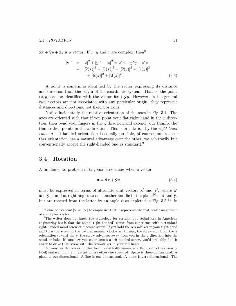
3.4. ROTATION 51
xx+ yy + zz is a vector. If x, y and z are complex, then8
|v|2 = |x|2 + |y|2 + |z|2 = x∗x+ y∗y + z∗z
= [<(x)]2 + [=(x)]2 + [<(y)]2 + [=(y)]2
+ [<(z)]2 + [=(z)]2 . (3.3)
A point is sometimes identified by the vector expressing its distanceand direction from the origin of the coordinate system. That is, the point(x, y) can be identified with the vector xx + yy. However, in the generalcase vectors are not associated with any particular origin; they representdistances and directions, not fixed positions.
Notice incidentally the relative orientation of the axes in Fig. 3.4. Theaxes are oriented such that if you point your flat right hand in the x direc-tion, then bend your fingers in the y direction and extend your thumb, thethumb then points in the z direction. This is orientation by the right-handrule. A left-handed orientation is equally possible, of course, but as nei-ther orientation has a natural advantage over the other, we arbitrarily butconventionally accept the right-handed one as standard.9
3.4 Rotation
A fundamental problem in trigonometry arises when a vector
u = xx+ yy (3.4)
must be expressed in terms of alternate unit vectors x′ and y′, where x′
and y′ stand at right angles to one another and lie in the plane10 of x and y,but are rotated from the latter by an angle ψ as depicted in Fig. 3.5.11 In
8Some books print |v| as ‖v‖ to emphasize that it represents the real, scalar magnitudeof a complex vector.
9The writer does not know the etymology for certain, but verbal lore in Americanengineering has it that the name “right-handed” comes from experience with a standardright-handed wood screw or machine screw. If you hold the screwdriver in your right handand turn the screw in the natural manner clockwise, turning the screw slot from the xorientation toward the y, the screw advances away from you in the z direction into thewood or hole. If somehow you came across a left-handed screw, you’d probably find iteasier to drive that screw with the screwdriver in your left hand.
10A plane, as the reader on this tier undoubtedly knows, is a flat (but not necessarilylevel) surface, infinite in extent unless otherwise specified. Space is three-dimensional. Aplane is two-dimensional. A line is one-dimensional. A point is zero-dimensional. The

52 CHAPTER 3. TRIGONOMETRY
Figure 3.5: Vector basis rotation.
x
y
ψ
ψ
x
y
x′y′
u
terms of the trigonometric functions of § 3.1, evidently
x′ = +x cosψ + y sinψ,
y′ = −x sinψ + y cosψ;(3.5)
and by appeal to symmetry it stands to reason that
x = +x′ cosψ − y′ sinψ,
y = +x′ sinψ + y′ cosψ.(3.6)
Substituting (3.6) into (3.4) yields
u = x′(x cosψ + y sinψ) + y′(−x sinψ + y cosψ), (3.7)
which was to be derived.
Equation (3.7) finds general application where rotations in rectangularcoordinates are involved. If the question is asked, “what happens if I rotatenot the unit basis vectors but rather the vector u instead?” the answer is
plane belongs to this geometrical hierarchy.11The “ ′ ” mark is pronounced “prime” or “primed” (for no especially good reason of
which the author is aware, but anyway, that’s how it’s pronounced). Mathematical writingemploys the mark for a variety of purposes. Here, the mark merely distinguishes the newunit vector x′ from the old x.

3.5. TRIGONOMETRIC SUMS AND DIFFERENCES 53
that it amounts to the same thing, except that the sense of the rotation isreversed:
u′ = x(x cosψ − y sinψ) + y(x sinψ + y cosψ). (3.8)
Whether it is the basis or the vector which rotates thus depends on yourpoint of view.12
3.5 Trigonometric functions of sums and differ-ences of angles
With the results of § 3.4 in hand, we now stand in a position to considertrigonometric functions of sums and differences of angles. Let
a ≡ x cosα+ y sinα,
b ≡ x cos β + y sinβ,
be vectors of unit length in the xy plane, respectively at angles α and βfrom the x axis. If we wanted b to coincide with a, we would have to rotateit by ψ = α − β. According to (3.8) and the definition of b, if we did thiswe would obtain
b′ = x[cos β cos(α− β)− sinβ sin(α− β)]+ y[cos β sin(α − β) + sinβ cos(α− β)].
Since we have deliberately chosen the angle of rotation such that b′ = a, wecan separately equate the x and y terms in the expressions for a and b′ toobtain the pair of equations
cosα = cos β cos(α− β)− sinβ sin(α− β),
sinα = cos β sin(α− β) + sinβ cos(α− β).
12This is only true, of course, with respect to the vectors themselves. When one actuallyrotates a physical body, the body experiences forces during rotation which might or mightnot change the body internally in some relevant way.

54 CHAPTER 3. TRIGONOMETRY
Solving the last pair simultaneously13 for sin(α − β) and cos(α − β) andobserving that sin2(·) + cos2(·) = 1 yields
sin(α− β) = sinα cos β − cosα sinβ,
cos(α− β) = cosα cos β + sinα sinβ.(3.9)
With the change of variable β ← −β and the observations from Table 3.1that sin(−φ) = − sinφ and cos(−φ) = +cos(φ), eqns. (3.9) become
sin(α+ β) = sinα cos β + cosα sinβ,
cos(α+ β) = cosα cos β − sinα sinβ.(3.10)
Equations (3.9) and (3.10) are the basic formulas for trigonometric functionsof sums and differences of angles.
3.5.1 Variations on the sums and differences
Several useful variations on (3.9) and (3.10) are achieved by combining theequations in various straightforward ways.14 These include
sinα sinβ =cos(α− β)− cos(α+ β)
2,
sinα cos β =sin(α− β) + sin(α+ β)
2,
cosα cos β =cos(α− β) + cos(α+ β)
2.
(3.11)
13The easy way to do this is
• to subtract sin β times the first equation from cos β times the second, then to solvethe result for sin(α − β);
• to add cos β times the first equation to sin β times the second, then to solve theresult for cos(α− β).
This shortcut technique for solving a pair of equations simultaneously for a pair of variablesis well worth mastering. In this book alone, it proves useful many times.
14Refer to footnote 13 above for the technique.

3.6. TRIGONOMETRICS OF THE HOUR ANGLES 55
With the change of variables δ ← α − β and γ ← α + β, (3.9) and (3.10)become
sin δ = sin
(
γ + δ
2
)
cos
(
γ − δ2
)
− cos
(
γ + δ
2
)
sin
(
γ − δ2
)
,
cos δ = cos
(
γ + δ
2
)
cos
(
γ − δ2
)
+ sin
(
γ + δ
2
)
sin
(
γ − δ2
)
,
sinγ = sin
(
γ + δ
2
)
cos
(
γ − δ2
)
+ cos
(
γ + δ
2
)
sin
(
γ − δ2
)
,
cos γ = cos
(
γ + δ
2
)
cos
(
γ − δ2
)
− sin
(
γ + δ
2
)
sin
(
γ − δ2
)
.
Combining these in various ways, we have that
sinγ + sin δ = 2 sin
(
γ + δ
2
)
cos
(
γ − δ2
)
,
sinγ − sin δ = 2 cos
(
γ + δ
2
)
sin
(
γ − δ2
)
,
cos δ + cos γ = 2 cos
(
γ + δ
2
)
cos
(
γ − δ2
)
,
cos δ − cos γ = 2 sin
(
γ + δ
2
)
sin
(
γ − δ2
)
.
(3.12)
3.5.2 Trigonometric functions of double and half angles
If α = β, then eqns. (3.10) become the double-angle formulas
sin 2α = 2 sinα cosα,
cos 2α = 2 cos2 α− 1 = cos2 α− sin2 α = 1− 2 sin2 α.(3.13)
Solving (3.13) for sin2 α and cos2 α yields the half-angle formulas
sin2 α =1− cos 2α
2,
cos2 α =1 + cos 2α
2.
(3.14)
3.6 Trigonometric functions of the hour angles
In general one uses the Taylor series of Ch. 8 to calculate trigonometricfunctions of specific angles. However, for angles which happen to be integral

56 CHAPTER 3. TRIGONOMETRY
multiples of an hour—there are twenty-four or 0x18 hours in a circle, justas there are twenty-four or 0x18 hours in a day15—for such angles simplerexpressions exist. Figure 3.6 shows the angles. Since such angles arise veryfrequently in practice, it seems worth our while to study them specially.
Table 3.2 tabulates the trigonometric functions of these hour angles. Tosee how the values in the table are calculated, look at the square and theequilateral triangle16 of Fig. 3.7. Each of the square’s four angles naturallymeasures six hours; and since a triangle’s angles always total twelve hours(§ 2.9.3), by symmetry each of the angles of the equilateral triangle in thefigure measures four. Also by symmetry, the perpendicular splits the trian-gle’s top angle into equal halves of two hours each and its bottom leg intoequal segments of length 1/2 each; and the diagonal splits the square’s cor-ner into equal halves of three hours each. The Pythagorean theorem (§ 2.10)then supplies the various other lengths in the figure, after which we observefrom Fig. 3.1 that
• the sine of a non-right angle in a right triangle is the opposite leg’slength divided by the diagonal’s,
15Hence an hour is 15, but you weren’t going to write your angles in such inelegantconventional notation as “15,” were you? Well, if you were, you’re in good company.
The author is fully aware of the barrier the unfamiliar notation poses for most first-timereaders of the book. The barrier is erected neither lightly nor disrespectfully. Consider:
• There are 0x18 hours in a circle.
• There are 360 degrees in a circle.
Both sentences say the same thing, don’t they? But even though the “0x” hex prefix isa bit clumsy, the first sentence nevertheless says the thing rather better. The reader isurged to invest the attention and effort to master the notation.
There is a psychological trap regarding the hour. The familiar, standard clock faceshows only twelve hours not twenty-four, so the angle between eleven o’clock and twelveon the clock face is not an hour of arc! That angle is two hours of arc. This is becausethe clock face’s geometry is artificial. If you have ever been to the Old Royal Observatoryat Greenwich, England, you may have seen the big clock face there with all twenty-fourhours on it. It’d be a bit hard to read the time from such a crowded clock face were it notso big, but anyway, the angle between hours on the Greenwich clock is indeed an honesthour of arc. [6]
The hex and hour notations are recommended mostly only for theoretical math work.It is not claimed that they offer much benefit in most technical work of the less theoret-ical kinds. If you wrote an engineering memo describing a survey angle as 0x1.80 hoursinstead of 22.5 degrees, for example, you’d probably not like the reception the memo got.Nonetheless, the improved notation fits a book of this kind so well that the author hazardsit. It is hoped that after trying the notation a while, the reader will approve the choice.
16An equilateral triangle is, as the name and the figure suggest, a triangle whose threesides all have the same length.

3.6. TRIGONOMETRICS OF THE HOUR ANGLES 57
Figure 3.6: The 0x18 hours in a circle.
Figure 3.7: A square and an equilateral triangle for calculating trigonometricfunctions of the hour angles.
1
1
√2
1 1
1/2 1/2
√3
2

58 CHAPTER 3. TRIGONOMETRY
Table 3.2: Trigonometric functions of the hour angles.
ANGLE φ[radians] [hours] sinφ tanφ cosφ
0 0 0 0 1
2π
0x181
√3− 1
2√
2
√3− 1√3 + 1
√3 + 1
2√
2
2π
0xC2
1
2
1√3
√3
2
2π
83
1√2
11√2
2π
64
√3
2
√3
1
2
(5)(2π)
0x185
√3 + 1
2√
2
√3 + 1√3− 1
√3− 1
2√
2
2π
46 1 ∞ 0

3.7. THE LAWS OF SINES AND COSINES 59
Figure 3.8: The laws of sines and cosines.
a
α
h
b c
γ β
y
x
• the tangent is the opposite leg’s length divided by the adjacent leg’s,and
• the cosine is the adjacent leg’s length divided by the diagonal’s.
With this observation and the lengths in the figure, one can calculate thesine, tangent and cosine of angles of two, three and four hours.
The values for one and five hours are found by applying (3.9) and (3.10)against the values for two and three hours just calculated. The values forzero and six hours are, of course, seen by inspection.17
3.7 The laws of sines and cosines
Refer to the triangle of Fig. 3.8. By the definition of the sine function, onecan write that
c sinβ = h = b sin γ,
or in other words that
sinβ
b=
sin γ
c.
17The creative reader may notice that he can extend the table to any angle by repeatedapplication of the various sum, difference and half-angle formulas from the precedingsections to the values already in the table. However, the Taylor series (§ 8.8) offers acleaner, quicker way to calculate trigonometrics of non-hour angles.

60 CHAPTER 3. TRIGONOMETRY
But there is nothing special about β and γ; what is true for them must betrue for α, too.18 Hence,
sinα
a=
sinβ
b=
sin γ
c. (3.15)
This equation is known as the law of sines.
On the other hand, if one expresses a and b as vectors emanating fromthe point γ,19
a = xa,
b = xb cos γ + yb sin γ,
then
c2 = |b− a|2
= (b cos γ − a)2 + (b sin γ)2
= a2 + (b2)(cos2 γ + sin2 γ)− 2ab cos γ.
Since cos2(·) + sin2(·) = 1, this is
c2 = a2 + b2 − 2ab cos γ. (3.16)
This equation is known as the law of cosines.
3.8 Summary of properties
Table 3.2 on page 58 has listed the values of trigonometric functions of thehour angles. Table 3.1 on page 48 has summarized simple properties of thetrigonometric functions. Table 3.3 summarizes further properties, gatheringthem from §§ 3.4, 3.5 and 3.7.
18“But,” it is objected, “there is something special about α. The perpendicular h dropsfrom it.”
True. However, the h is just a utility variable to help us to manipulate the equationinto the desired form; we’re not interested in h itself. Nothing prevents us from droppingadditional perpendiculars hβ and hγ from the other two corners and using those as utilityvariables, too, if we like. We can use any utility variables we want.
19Here is another example of the book’s judicious relaxation of formal rigor. Of coursethere is no “point γ”; γ is an angle not a point. However, the writer suspects in light ofFig. 3.8 that few readers will be confused as to which point is meant. The skillful appliedmathematician does not multiply labels without need.

3.8. SUMMARY OF PROPERTIES 61
Table 3.3: Further properties of the trigonometric functions.
u = x′(x cosψ + y sinψ) + y′(−x sinψ + y cosψ)
sin(α± β) = sinα cos β ± cosα sinβ
cos(α± β) = cosα cos β ∓ sinα sinβ
sinα sinβ =cos(α− β)− cos(α+ β)
2
sinα cos β =sin(α− β) + sin(α+ β)
2
cosα cos β =cos(α− β) + cos(α+ β)
2
sin γ + sin δ = 2 sin
(
γ + δ
2
)
cos
(
γ − δ2
)
sin γ − sin δ = 2 cos
(
γ + δ
2
)
sin
(
γ − δ2
)
cos δ + cos γ = 2 cos
(
γ + δ
2
)
cos
(
γ − δ2
)
cos δ − cos γ = 2 sin
(
γ + δ
2
)
sin
(
γ − δ2
)
sin 2α = 2 sinα cosα
cos 2α = 2 cos2 α− 1 = cos2 α− sin2 α = 1− 2 sin2 α
sin2 α =1− cos 2α
2
cos2 α =1 + cos 2α
2sin γ
c=
sinα
a=
sinβ
bc2 = a2 + b2 − 2ab cos γ

62 CHAPTER 3. TRIGONOMETRY
3.9 Cylindrical and spherical coordinates
Section 3.3 has introduced the concept of the vector
v = xx+ yy + zz.
The coefficients (x, y, z) on the equation’s right side are coordinates—specif-ically, rectangular coordinates—which given a specific orthonormal20 set ofunit basis vectors [x y z] uniquely identify a point (see Fig. 3.4 on page 49).Such rectangular coordinates are simple and general, and are convenient formany purposes. However, there are at least two broad classes of conceptuallysimple problems for which rectangular coordinates tend to be inconvenient:problems in which an axis or a point dominates. Consider for example anelectric wire’s magnetic field, whose intensity varies with distance from thewire (an axis); or the illumination a lamp sheds on a printed page of thisbook, which depends on the book’s distance from the lamp (a point).
To attack a problem dominated by an axis, the cylindrical coordinates(ρ;φ, z) can be used instead of the rectangular coordinates (x, y, z). Toattack a problem dominated by a point, the spherical coordinates (r; θ;φ)can be used.21 Refer to Fig. 3.9. Such coordinates are related to one anotherand to the rectangular coordinates by the formulas of Table 3.4.
Cylindrical and spherical coordinates can greatly simplify the analyses ofthe kinds of problems they respectively fit, but they come at a price. Thereare no constant unit basis vectors to match them. That is,
v = xx+ yy + zz 6= ρρ+ φφ+ zz 6= rr + θθ + φφ.
It doesn’t work that way. Nevertheless variable unit basis vectors are de-fined:
ρ ≡ +x cosφ+ y sinφ,
φ ≡ −x sinφ + y cosφ,
r ≡ +z cos θ + ρ sin θ,
θ ≡ −z sin θ + ρ cos θ.
(3.17)
Such variable unit basis vectors point locally in the directions in which theirrespective coordinates advance.
20Orthonormal in this context means “of unit length and at right angles to the othervectors in the set.” [3, “Orthonormality,” 14:19, 7 May 2006]
21Notice that the φ is conventionally written second in cylindrical (ρ;φ, z) but third inspherical (r; θ;φ) coordinates. This odd-seeming convention is to maintain proper right-handed coordinate rotation. It will be clearer after reading Ch. [not yet written].

3.9. CYLINDRICAL AND SPHERICAL COORDINATES 63
Figure 3.9: A point on a sphere, in spherical (r; θ;φ) and cylindrical (ρ;φ, z)coordinates. (The axis labels bear circumflexes in this figure only to disam-biguate the z axis from the cylindrical coordinate z.)
rθ
φ
ρ
z
z
y
x
Table 3.4: Relations among the rectangular, cylindrical and spherical coor-dinates.
ρ2 = x2 + y2
r2 = ρ2 + z2 = x2 + y2 + z2
tan θ =ρ
z
tanφ =y
xz = r cos θ
ρ = r sin θ
x = ρ cosφ = r sin θ cosφ
y = ρ sinφ = r sin θ sinφ

64 CHAPTER 3. TRIGONOMETRY
Convention usually orients z in the direction of a problem’s axis. Occa-sionally however a problem arises in which it is more convenient to orient xor y in the direction of the problem’s axis (usually because z has alreadybeen established in the direction of some other pertinent axis). Changingthe meanings of known symbols like ρ, θ and φ is usually not a good idea,but you can use symbols like
ρ2x = y2 + z2, ρ2
y = z2 + x2,
tan θx =ρxx, tan θy =
ρyy,
tanφx =z
y, tanφy =
x
z,
(3.18)
instead if needed.22
3.10 The complex triangle inequalities
If a, b and c represent the three sides of a triangle such that a + b + c = 0,then per (2.44)
|a| − |b| ≤ |a + b| ≤ |a|+ |b| .
These are just the triangle inequalities of § 2.9.2 in vector notation. But ifthe triangle inequalities hold for vectors in a plane, then why not equallyfor complex numbers? Consider the geometric interpretation of the Argandplane of Fig. 2.5 on page 40. Evidently,
|z1| − |z2| ≤ |z1 + z2| ≤ |z1|+ |z2| (3.19)
for any two complex numbers z1 and z2. Extending the sum inequality, wehave that
∣
∣
∣
∣
∣
∑
k
zk
∣
∣
∣
∣
∣
≤∑
k
|zk| . (3.20)
Naturally, (3.19) and (3.20) hold equally well for real numbers as for com-plex; one may find the latter formula useful for sums of real numbers, forexample, when some of the numbers summed are positive and others nega-tive.
22Symbols like ρx are logical but, as far as this writer is aware, not standard. The writeris not aware of any conventionally established symbols for quantities like these.

3.11. DE MOIVRE’S THEOREM 65
An important consequence of (3.20) is that if∑ |zk| converges, then
∑
zk also converges. Such a consequence is important because mathematicalderivations sometimes need the convergence of
∑
zk established, which canbe hard to do directly. Convergence of
∑ |zk|, which per (3.20) impliesconvergence of
∑
zk, is often easier to establish.
Equation (3.20) will find use among other places in § 8.9.3.
3.11 De Moivre’s theorem
Compare the Argand-plotted complex number of Fig. 2.5 (page 40) againstthe vector of Fig. 3.3 (page 49). Although complex numbers are scalars notvectors, the figures do suggest an analogy between complex phase and vectordirection. With reference to Fig. 2.5 we can write
z = (ρ)(cos φ+ i sinφ) = ρ cisφ, (3.21)
where
cisφ ≡ cosφ+ i sinφ. (3.22)
If z = x+ iy, then evidently
x = ρ cosφ,
y = ρ sinφ.(3.23)
Per (2.53),
z1z2 = (x1x2 − y1y2) + i(y1x2 + x1y2).
Applying (3.23) to the equation yields
z1z2ρ1ρ2
= (cosφ1 cosφ2 − sinφ1 sinφ2) + i(sinφ1 cosφ2 + cosφ1 sinφ2).
But according to (3.10), this is just
z1z2ρ1ρ2
= cos(φ1 + φ2) + i sin(φ1 + φ2),
or in other words
z1z2 = ρ1ρ2 cis(φ1 + φ2). (3.24)
Equation (3.24) is an important result. It says that if you want to multiplycomplex numbers, it suffices

66 CHAPTER 3. TRIGONOMETRY
• to multiply their magnitudes and
• to add their phases.
It follows by parallel reasoning (or by extension) that
z1z2
=ρ1
ρ2cis(φ1 − φ2) (3.25)
and by extension thatza = ρa cis aφ. (3.26)
Equations (3.24), (3.25) and (3.26) are known as de Moivre’s theorem.23 ,24
We have not shown it yet, but in § 5.4 we shall show that
cisφ = exp iφ = eiφ,
where exp(·) is the natural exponential function and e is the natural loga-rithmic base, both defined in Ch. 5. De Moivre’s theorem is most useful inlight of this.
23Also called de Moivre’s formula. Some authors apply the name of de Moivre directlyonly to (3.26), or to some variation thereof; but as the three equations express essentiallythe same idea, if you refer to any of them as de Moivre’s theorem then you are unlikelyto be misunderstood.
24[35][3]

Chapter 4
The derivative
The mathematics of calculus concerns a complementary pair of questions:1
• Given some function f(t), what is the function’s instantaneous rate ofchange, or derivative, f ′(t)?
• Interpreting some function f ′(t) as an instantaneous rate of change,what is the corresponding accretion, or integral, f(t)?
This chapter builds toward a basic understanding of the first question.
4.1 Infinitesimals and limits
Calculus systematically treats numbers so large and so small, they lie beyondthe reach of our mundane number system.
1Although once grasped the concept is relatively simple, to understand this pair ofquestions, so briefly stated, is no trivial thing. They are the pair which eluded or con-founded the most brilliant mathematical minds of the ancient world.
The greatest conceptual hurdle—the stroke of brilliance—probably lies simply in statingthe pair of questions clearly. Sir Isaac Newton and G.W. Leibnitz cleared this hurdle forus in the seventeenth century, so now at least we know the right pair of questions to ask.With the pair in hand, the calculus beginner’s first task is quantitatively to understandthe pair’s interrelationship, generality and significance. Such an understanding constitutesthe basic calculus concept.
It cannot be the role of a book like this one to lead the beginner gently toward anapprehension of the basic calculus concept. Once grasped, the concept is simple andbriefly stated. In this book we necessarily state the concept briefly, then move along.Many instructional textbooks—[19] is a worthy example—have been written to lead thebeginner gently. Although a sufficiently talented, dedicated beginner could perhaps obtainthe basic calculus concept directly here, he would probably find it quicker and morepleasant to begin with a book like the one referenced.
67

68 CHAPTER 4. THE DERIVATIVE
4.1.1 The infinitesimal
A number ε is an infinitesimal if it is so small that
0 < |ε| < a
for all possible mundane positive numbers a.This is somewhat a difficult concept, so if it is not immediately clear
then let us approach the matter colloquially. Let me propose to you that Ihave an infinitesimal.
“How big is your infinitesimal?” you ask.“Very, very small,” I reply.“How small?”“Very small.”“Smaller than 0x0.01?”“Smaller than what?”“Than 2−8. You said that we should use hexadecimal notation in this
book, remember?”“Sorry. Yes, right, smaller than 0x0.01.”“What about 0x0.0001? Is it smaller than that?”“Much smaller.”“Smaller than 0x0.0000 0000 0000 0001?”“Smaller.”“Smaller than 2−0x1 0000 0000 0000 0000?”“Now that is an impressively small number. Nevertheless, my infinitesi-
mal is smaller still.”“Zero, then.”“Oh, no. Bigger than that. My infinitesimal is definitely bigger than
zero.”This is the idea of the infinitesimal. It is a definite number of a certain
nonzero magnitude, but its smallness conceptually lies beyond the reach ofour mundane number system.
If ε is an infinitesimal, then 1/ε can be regarded as an infinity: a verylarge number much larger than any mundane number one can name.
The principal advantage of using symbols like ε rather than 0 for in-finitesimals is in that it permits us conveniently to compare one infinitesimalagainst another, to add them together, to divide them, etc. For instance,if δ = 3ε is another infinitesimal, then the quotient δ/ε is not some unfath-omable 0/0; rather it is δ/ε = 3. In physical applications, the infinitesimalsare often not true mathematical infinitesimals but rather relatively verysmall quantities such as the mass of a wood screw compared to the mass

4.1. INFINITESIMALS AND LIMITS 69
of a wooden house frame, or the audio power of your voice compared tothat of a jet engine. The additional cost of inviting one more guest to thewedding may or may not be infinitesimal, depending on your point of view.The key point is that the infinitesimal quantity be negligible by comparison,whatever “negligible” means in the context.2
The second-order infinitesimal ε2 is so small on the scale of the common,first-order infinitesimal ε that the even latter cannot measure it. The ε2 isan infinitesimal to the infinitesimals. Third- and higher-order infinitesimalsare likewise possible.
The notation u v, or v u, indicates that u is much less than v,typically such that one can regard the quantity u/v to be an infinitesimal.In fact, one common way to specify that ε be infinitesimal is to write thatε 1.
4.1.2 Limits
The notation limz→zo indicates that z draws as near to zo as it possiblycan. When written limz→z+o
, the implication is that z draws toward zo fromthe positive side such that z > zo. Similarly, when written limz→z−o
, theimplication is that z draws toward zo from the negative side.
The reason for the notation is to provide a way to handle expressionslike
3z
2z
as z vanishes:
limz→0
3z
2z=
3
2.
The symbol “limQ” is short for “in the limit as Q.”
Notice that lim is not a function like log or sin. It is just a reminderthat a quantity approaches some value, used when saying that the quantity
2Among scientists and engineers who study wave phenomena, there is an old ruleof thumb that sinusoidal waveforms be discretized not less finely than ten points perwavelength. In keeping with this book’s adecimal theme (Appendix A) and the concept ofthe hour of arc (§ 3.6), we should probably render the rule as twelve points per wavelengthhere. In any case, even very roughly speaking, a quantity greater then 1/0xC of theprincipal to which it compares probably cannot rightly be regarded as infinitesimal. On theother hand, a quantity less than 1/0x10000 of the principal is indeed infinitesimal for mostpractical purposes (but not all: for example, positions of spacecraft and concentrations ofchemical impurities must sometimes be accounted more precisely). For quantities between1/0xC and 1/0x10000, it depends on the accuracy one seeks.

70 CHAPTER 4. THE DERIVATIVE
equaled the value would be confusing. Consider that to say
limz→2−
(z + 2) = 4
is just a fancy way of saying that 2 + 2 = 4. The lim notation is convenientto use sometimes, but it is not magical. Don’t let it confuse you.
4.2 Combinatorics
In its general form, the problem of selecting k specific items out of a set of navailable items belongs to probability theory ([chapter not yet written]). Inits basic form, however, the same problem also applies to the handling ofpolynomials or power series. This section treats the problem in its basicform.3
4.2.1 Combinations and permutations
Consider the following scenario. I have several small wooden blocks of var-ious shapes and sizes, painted different colors so that you can clearly telleach block from the others. If I offer you the blocks and you are free to takeall, some or none of them at your option, if you can take whichever blocksyou want, then how many distinct choices of blocks do you have? Answer:you have 2n choices, because you can accept or reject the first block, thenaccept or reject the second, then the third, and so on.
Now, suppose that what you want is exactly k blocks, neither more norfewer. Desiring exactly k blocks, you select your favorite block first: thereare n options for this. Then you select your second favorite: for this, thereare n− 1 options (why not n options? because you have already taken oneblock from me; I have only n − 1 blocks left). Then you select your thirdfavorite—for this there are n−2 options—and so on until you have k blocks.There are evidently
P
(
nk
)
≡ n!/(n− k)! (4.1)
ordered ways, or permutations, available for you to select exactly k blocks.
However, some of these distinct permutations result in putting exactlythe same combination of blocks in your pocket; for instance, the permu-tations red-green-blue and green-red-blue constitute the same combination,
3[19]

4.2. COMBINATORICS 71
whereas red-white-blue is a different combination entirely. For a single com-bination of k blocks (red, green, blue), evidently k! permutations are possi-ble (red-green-blue, red-blue-green, green-red-blue, green-blue-red, blue-red-green, blue-green-red). Hence dividing the number of permutations (4.1)by k! yields the number of combinations
(
nk
)
≡ n!/(n− k)!k!
. (4.2)
Properties of the number„
nk
«
of combinations include that
(
nn− k
)
=
(
nk
)
, (4.3)
n∑
k=0
(
nk
)
= 2n, (4.4)
(
n− 1k − 1
)
+
(
n− 1k
)
=
(
nk
)
, (4.5)
(
nk
)
=n− k + 1
k
(
nk − 1
)
(4.6)
=k + 1
n− k
(
nk + 1
)
(4.7)
=n
k
(
n− 1k − 1
)
(4.8)
=n
n− k
(
n− 1k
)
. (4.9)
Equation (4.3) results from changing the variable k ← n− k in (4.2). Equa-tion (4.4) comes directly from the observation (made at the head of thissection) that 2n total combinations are possible if any k is allowed. Equa-tion (4.5) is seen when an nth block—let us say that it is a black block—isadded to an existing set of n − 1 blocks; to choose k blocks then, you caneither choose k from the original set, or the black block plus k− 1 from theoriginal set. Equations (4.6) through (4.9) come directly from the defini-tion (4.2); they relate combinatoric coefficients to their neighbors in Pascal’striangle (§ 4.2.2).
Because one cannot choose fewer than zero or more than n from n blocks,(
nk
)
= 0 unless 0 ≤ k ≤ n. (4.10)

72 CHAPTER 4. THE DERIVATIVE
Figure 4.1: The plan for Pascal’s triangle.
„
00
«
„
10
«„
11
«
„
20
«„
21
«„
22
«
„
30
«„
31
«„
32
«„
33
«
„
40
«„
41
«„
42
«„
43
«„
44
«
...
For„
nk
«
when n < 0, there is no obvious definition.
4.2.2 Pascal’s triangle
Consider the triangular layout in Fig. 4.1 of the various possible„
nk
«
.
Evaluated, this yields Fig. 4.2, Pascal’s triangle. Notice how each entryin the triangle is the sum of the two entries immediately above, as (4.5)predicts. (In fact this is the easy way to fill Pascal’s triangle out: for eachentry, just add the two entries above.)
4.3 The binomial theorem
This section presents the binomial theorem and one of its significant conse-quences.
4.3.1 Expanding the binomial
The binomial theorem holds that4
(a+ b)n =n∑
k=0
(
nk
)
an−kbk. (4.11)
4The author is given to understand that, by an heroic derivational effort, (4.11) can beextended to nonintegral n. However, since applied mathematics does not usually concernitself with hard theorems of little known practical use, the extension is not covered in thisbook.

4.3. THE BINOMIAL THEOREM 73
Figure 4.2: Pascal’s triangle.
11 1
1 2 11 3 3 1
1 4 6 4 11 5 A A 5 1
1 6 F 14 F 6 11 7 15 23 23 15 7 1
...
In the common case a = 1, b = ε 1, this is
(1 + ε)n =
n∑
k=0
(
nk
)
εk (4.12)
(actually this holds for any ε, small or large; but the typical case of interestis ε 1). In either form, the binomial theorem is a direct consequence ofthe combinatorics of § 4.2. Since
(a+ b)n = (a+ b)(a+ b) · · · (a+ b)(a+ b),
each (a+b) factor corresponds to one of the “wooden blocks,” where a meansrejecting the block and b, accepting it.
4.3.2 Powers of numbers near unity
Since„
n0
«
= 1 and„
n1
«
= n, it follows from (4.12) that
(1 + εo)n ≈ 1 + nεo,
to excellent precision for nonnegative integral n if εo is sufficiently small.Furthermore, raising the equation to the 1/n power then changing δ ← nεoand m← n, we have that
(1 + δ)1/m ≈ 1 +δ
m.

74 CHAPTER 4. THE DERIVATIVE
Changing 1 + δ ← (1 + ε)n and observing from the (1 + εo)n equation above
that this implies that δ ≈ nε, we have that
(1 + ε)n/m ≈ 1 +n
mε.
Inverting this equation yields
(1 + ε)−n/m ≈ 1
1 + (n/m)ε=
[1− (n/m)ε]
[1− (n/m)ε][1 + (n/m)ε]≈ 1− n
mε.
Taken together, the last two equations imply that
(1 + ε)x ≈ 1 + xε (4.13)
for any real x.
The writer knows of no conventional name5 for (4.13), but named orunnamed it is an important equation. The equation offers a simple, accurateway of approximating any real power of numbers in the near neighborhoodof 1.
4.3.3 Complex powers of numbers near unity
Equation (4.13) raises the question: what if ε or x, or both, are complex?Changing the symbol z ← x and observing that the infinitesimal ε may alsobe complex, one wants to know whether
(1 + ε)z ≈ 1 + zε (4.14)
still holds. No work we have yet done in the book answers the question,because although a complex infinitesimal ε poses no particular problem, theaction of a complex power z remains undefined. Still, for consistency’s sake,one would like (4.14) to hold. In fact nothing prevents us from defining theaction of a complex power such that (4.14) does hold, which we now do,logically extending the known result (4.13) into the new domain.
Section 5.4 will investigate the extremely interesting effects which arisewhen <(ε) = 0 and the power z in (4.14) grows large, but for the momentwe shall use the equation in a more ordinary manner to develop the conceptand basic application of the derivative, as follows.
5Other than “the first-order Taylor expansion,” but such an unwieldy name does notfit the present context. The Taylor expansion as such will be introduced later (Ch. 8).

4.4. THE DERIVATIVE 75
4.4 The derivative
With (4.14) in hand, we now stand in a position to introduce the derivative.What is the derivative? The derivative is the instantaneous rate or slope of afunction. In mathematical symbols and for the moment using real numbers,
f ′(t) ≡ limε→0+
f(t+ ε/2)− f(t− ε/2)ε
. (4.15)
Alternately, one can define the same derivative in the unbalanced form
f ′(t) = limε→0+
f(t+ ε)− f(t)
ε,
but this book generally prefers the more elegant balanced form (4.15), whichwe will now use in developing the derivative’s several properties through therest of the chapter.6
4.4.1 The derivative of the power series
In the very common case that f(t) is the power series
f(t) =∞∑
k=−∞ckt
k, (4.16)
where the ck are in general complex coefficients, (4.15) says that
f ′(t) =∞∑
k=−∞limε→0+
(ck)(t+ ε/2)k − (ck)(t− ε/2)kε
=∞∑
k=−∞limε→0+
cktk (1 + ε/2t)k − (1− ε/2t)k
ε.
Applying (4.14), this is
f ′(t) =
∞∑
k=−∞limε→0+
cktk (1 + kε/2t)− (1− kε/2t)
ε,
which simplifies to
f ′(t) =
∞∑
k=−∞ckkt
k−1. (4.17)
6From this section through § 4.7, the mathematical notation grows a little thick. Thereis no helping this. The reader is advised to tread through these sections line by stubbornline, in the good trust that the math thus gained will prove both interesting and useful.

76 CHAPTER 4. THE DERIVATIVE
Equation (4.17) gives the general derivative of the power series.7
4.4.2 The Leibnitz notation
The f ′(t) notation used above for the derivative is due to Sir Isaac New-ton, and is easier to start with. Usually better on the whole, however, isG.W. Leibnitz’s notation8
dt = ε,
df = f(t+ dt/2)− f(t− dt/2),
such that per (4.15),
f ′(t) =df
dt. (4.18)
Here dt is the infinitesimal, and df is a dependent infinitesimal whose sizerelative to dt depends on the independent variable t. For the independentinfinitesimal dt, conceptually, one can choose any infinitesimal size ε. Usu-ally the exact choice of size doesn’t matter, but occasionally when there aretwo independent variables it helps the analysis to adjust the size of one ofthe independent infinitesimals with respect to the other.
The meaning of the symbol d unfortunately depends on the context.In (4.18), the meaning is clear enough: d(·) signifies how much (·) changeswhen the independent variable t increments by dt.9 Notice, however, thatthe notation dt itself has two distinct meanings:10
7Equation (4.17) admittedly has not explicitly considered what happens when the real tbecomes the complex z, but § 4.4.3 will remedy the oversight.
8This subsection is likely to confuse many readers the first time they read it. The reasonis that Leibnitz elements like dt and ∂f usually tend to appear in practice in certain specificrelations to one another, like ∂f/∂z. As a result, many users of applied mathematicshave never developed a clear understanding as to precisely what the individual symbolsmean. Often they have developed positive misunderstandings. Because there is significantpractical benefit in learning how to handle the Leibnitz notation correctly—particularly inapplied complex variable theory—this subsection seeks to present each Leibnitz elementin its correct light.
9If you do not fully understand this sentence, reread it carefully with reference to (4.15)and (4.18) until you do; it’s important.
10This is difficult, yet the author can think of no clearer, more concise way to state it.The quantities dt and df represent coordinated infinitesimal changes in t and f respectively,so there is usually no trouble with treating dt and df as though they were the same kindof thing. However, at the fundamental level they really aren’t.
If t is an independent variable, then dt is just an infinitesimal of some kind, whosespecific size could be a function of t but more likely is just a constant. If a constant,then dt does not fundamentally have anything to do with t as such. In fact, if s and t

4.4. THE DERIVATIVE 77
• the independent infinitesimal dt = ε; and
• d(t), which is how much (t) changes as t increments by dt.
At first glance, the distinction between dt and d(t) seems a distinction with-out a difference; and for most practical cases of interest, so indeed it is.However, when switching perspective in mid-analysis as to which variablesare dependent and which are independent, or when changing multiple inde-pendent complex variables simultaneously, the math can get a little tricky.In such cases, it may be wise to use the symbol dt to mean d(t) only, in-troducing some unambiguous symbol like ε to represent the independentinfinitesimal. In any case you should appreciate the conceptual differencebetween dt = ε and d(t).
are both independent variables, then we can (and in complex analysis sometimes do) saythat ds = dt = ε, after which nothing prevents us from using the symbols ds and dtinterchangeably. Maybe it would be clearer in some cases to write ε instead of dt, but thelatter is how it is conventionally written.
By contrast, if f is a dependent variable, then df or d(f) is the amount by which fchanges as t changes by dt. The df is infinitesimal but not constant; it is a function of t.Maybe it would be clearer in some cases to write dtf instead of df , but for most cases theformer notation is unnecessarily cluttered; the latter is how it is conventionally written.
Now, most of the time, what we are interested in is not dt or df as such, but rather theratio df/dt or the sum
P
k f(k dt) dt =R
f(t) dt. For this reason, we do not usually worryabout which of df and dt is the independent infinitesimal, nor do we usually worry aboutthe precise value of dt. This leads one to forget that dt does indeed have a precise value.What confuses is when one changes perspective in mid-analysis, now regarding f as theindependent variable. Changing perspective is allowed and perfectly proper, but one musttake care: the dt and df after the change are not the same as the dt and df before thechange. However, the ratio df/dt remains the same in any case.
Sometimes when writing a differential equation like the potential-kinetic energy equationmadx = mv dv, we do not necessarily have either v or x in mind as the independentvariable. This is fine. The important point is that dv and dx be coordinated so that theratio dv/dx has a definite value no matter which of the two be regarded as independent,or whether the independent be some third variable (like t) not in the equation.
One can avoid the confusion simply by keeping the dv/dx or df/dt always in ratio, nevertreating the infinitesimals individually. Many applied mathematicians do precisely that.That is okay as far as it goes, but it really denies the entire point of the Leibnitz notation.One might as well just stay with the Newton notation in that case. Instead, this writerrecommends that you learn the Leibnitz notation properly, developing the ability to treatthe infinitesimals individually.
Because the book is a book of applied mathematics, this footnote does not attempt tosay everything there is to say about infinitesimals. For instance, it has not yet pointedout (but does so now) that even if s and t are equally independent variables, one can havedt = ε(t), ds = δ(s, t), such that dt has prior independence to ds. The point is not tofathom all the possible implications from the start; you can do that as the need arises.The point is to develop a clear picture in your mind of what a Leibnitz infinitesimal reallyis. Once you have the picture, you can go from there.

78 CHAPTER 4. THE DERIVATIVE
Where two or more independent variables are at work in the same equa-tion, it is conventional to use the symbol ∂ instead of d, as a reminder thatthe reader needs to pay attention to which ∂ tracks which independent vari-able.11 (If needed or desired, one can write ∂t(·) when tracking t, ∂s(·) whentracking s, etc. You have to be careful, though. Such notation appears onlyrarely in the literature, so your audience might not understand it when youwrite it.) Conventional shorthand for d(df) is d2f ; for (dt)2, dt2; so
d(df/dt)
dt=d2f
dt2
is a derivative of a derivative, or second derivative. By extension, the nota-tion
dkf
dtk
represents the kth derivative.
4.4.3 The derivative of a function of a complex variable
For (4.15) to be robust, written here in the slightly more general form
df
dz= lim
ε→0
f(z + ε/2) − f(z − ε/2)ε
, (4.19)
one should like it to evaluate the same in the limit regardless of the complexphase of ε. That is, if δ is a positive real infinitesimal, then it should beequally valid to let ε = δ, ε = −δ, ε = iδ, ε = −iδ, ε = (4 − i3)δ orany other infinitesimal value, so long as 0 < |ε| 1. One should like thederivative (4.19) to come out the same regardless of the Argand directionfrom which ε approaches 0 (see Fig. 2.5). In fact for the sake of robustness,one normally demands that derivatives do come out the same regardlessof the Argand direction; and (4.19) rather than (4.15) is the definition wenormally use for the derivative for this reason. Where the limit (4.19) issensitive to the Argand direction or complex phase of ε, there we normallysay that the derivative does not exist.
Where the derivative (4.19) does exist—where the derivative is finiteand insensitive to Argand direction—there we say that the function f(z) isdifferentiable.
Excepting the nonanalytic parts of complex numbers (|·|, arg(·), (·)∗,<(·) and =(·); see § 2.12.3), plus the Heaviside unit step u(t) and the Dirac
11The writer confesses that he remains unsure why this minor distinction merits theseparate symbol ∂, but he accepts the notation as conventional nevertheless.

4.4. THE DERIVATIVE 79
delta δ(t) (§ 7.7), most functions encountered in applications do meet the cri-terion (4.19) except at isolated nonanalytic points (like z = 0 in h(z) = 1/zor g(z) =
√z). Meeting the criterion, such functions are fully differentiable
except at their poles (where the derivative goes infinite in any case) andother nonanalytic points. Particularly, the key formula (4.14), written hereas
(1 + ε)w ≈ 1 + wε,
works without modification when ε is complex; so the derivative (4.17) ofthe general power series,
d
dz
∞∑
k=−∞ckz
k =∞∑
k=−∞ckkz
k−1 (4.20)
holds equally well for complex z as for real.
4.4.4 The derivative of za
Inspection of § 4.4.1’s logic in light of (4.14) reveals that nothing prevents usfrom replacing the real t, real ε and integral k of that section with arbitrarycomplex z, ε and a. That is,
d(za)
dz= lim
ε→0
(z + ε/2)a − (z − ε/2)aε
= limε→0
za(1 + ε/2z)a − (1− ε/2z)a
ε
= limε→0
za(1 + aε/2z)− (1− aε/2z)
ε,
which simplifies tod(za)
dz= aza−1 (4.21)
for any complex z and a.How exactly to evaluate za or za−1 when a is complex is another matter,
treated in § 5.4 and its (5.12); but in any case you can use (4.21) for real aright now.
4.4.5 The logarithmic derivative
Sometimes one is more interested in knowing the rate of f(t) relative tothe value of f(t) than in knowing the absolute rate itself. For example, ifyou inform me that you earn $ 1000 a year on a bond you hold, then I may

80 CHAPTER 4. THE DERIVATIVE
commend you vaguely for your thrift but otherwise the information does nottell me much. However, if you inform me instead that you earn 10 percenta year on the same bond, then I might want to invest. The latter figure isa relative rate, or logarithmic derivative,
df/dt
f(t)=
d
dtln f(t). (4.22)
The investment principal grows at the absolute rate df/dt, but the bond’sinterest rate is (df/dt)/f(t).
The natural logarithmic notation ln f(t) may not mean much to you yet,as we’ll not introduce it formally until § 5.2, so you can ignore the right sideof (4.22) for the moment; but the equation’s left side at least should makesense to you. It expresses the significant concept of a relative rate, like 10percent annual interest on a bond.
4.5 Basic manipulation of the derivative
This section introduces the derivative chain and product rules.
4.5.1 The derivative chain rule
If f is a function of w, which itself is a function of z, then12
df
dz=
(
df
dw
)(
dw
dz
)
. (4.23)
12For example, one can rewrite
f(z) =p
3z2 − 1
in the form
f(w) = w1/2,
w(z) = 3z2 − 1.
Then
df
dw=
1
2w1/2=
1
2√
3z2 − 1,
dw
dz= 6z,
so by (4.23),df
dz=
„
df
dw
« „
dw
dz
«
=6z
2√
3z2 − 1=
3z√3z2 − 1
.

4.5. BASIC MANIPULATION OF THE DERIVATIVE 81
Equation (4.23) is the derivative chain rule.13
4.5.2 The derivative product rule
In general per (4.19),
d
∏
j
fj(z)
=∏
j
fj
(
z +dz
2
)
−∏
j
fj
(
z − dz
2
)
.
But to first order,
fj
(
z ± dz
2
)
≈ fj(z)±(
dfjdz
)(
dz
2
)
= fj(z) ±dfj2,
so in the limit,
d
∏
j
fj(z)
=∏
j
(
fj(z) +dfj2
)
−∏
j
(
fj(z)−dfj2
)
.
Since the product of two or more dfj is negligible compared to the first-orderinfinitesimals to which they are added here, this simplifies to
d
∏
j
fj(z)
=
∏
j
fj(z)
[
∑
k
dfk2fk(z)
]
−
∏
j
fj(z)
[
∑
k
−dfk2fk(z)
]
,
or in other words
d∏
j
fj =
∏
j
fj
[
∑
k
dfkfk
]
. (4.24)
In the common case of only two fj, this comes to
d(f1f2) = f2 df1 + f1 df2. (4.25)
On the other hand, if f1(z) = f(z) and f2(z) = 1/g(z), then by the derivativechain rule (4.23), df2 = −dg/g2; so,
d
(
f
g
)
=g df − f dg
g2. (4.26)
13It bears emphasizing to readers who may inadvertently have picked up unhelpful ideasabout the Leibnitz notation in the past: the dw factor in the denominator cancels the dwfactor in the numerator; a thing divided by itself is 1. That’s it. There is nothing moreto the proof of the derivative chain rule than that.

82 CHAPTER 4. THE DERIVATIVE
Equation (4.24) is the derivative product rule.After studying the complex exponential in Ch. 5, we shall stand in a
position to write (4.24) in the slightly specialized but often useful form14
d
∏
j
gaj
j
∏
j
ebjhj∏
j
ln cjpj
=
∏
j
gaj
j
∏
j
ebjhj∏
j
ln cjpj
×[
∑
k
akdgkgk
+∑
k
bk dhk +∑
k
dpkpk ln ckpk
]
. (4.27)
where the ak and bk are arbitrary complex coefficients and the gk and hkare arbitrary functions.15
4.6 Extrema and higher derivatives
One problem which arises very frequently in applied mathematics is theproblem of finding a local extremum—that is, a local minimum or max-imum—of a real-valued function f(x). Refer to Fig. 4.3. The almost dis-tinctive characteristic of the extremum xo is that16
df
dx
∣
∣
∣
∣
x=xo
= 0. (4.28)
At the extremum, the slope is zero. The curve momentarily runs level there.One solves (4.28) to find the extremum.
Whether the extremum be a minimum or a maximum depends on wheth-er the curve turn from a downward slope to an upward, or from an upwardslope to a downward, respectively. If from downward to upward, then thederivative of the slope is evidently positive; if from upward to downward,
14This paragraph is extra. You can skip it for now if you prefer.15The subsection is sufficiently abstract that it is a little hard to understand unless one
already knows what it means. An example may help:
d
»
u2v3
ze−5t ln 7s
–
=
»
u2v3
ze−5t ln 7s
– »
2du
u+ 3
dv
v− dz
z− 5 dt+
ds
s ln 7s
–
.
16The notation P |Q means “P when Q,” “P , given Q,” or “P evaluated at Q.” Some-times it is alternately written P |Q.
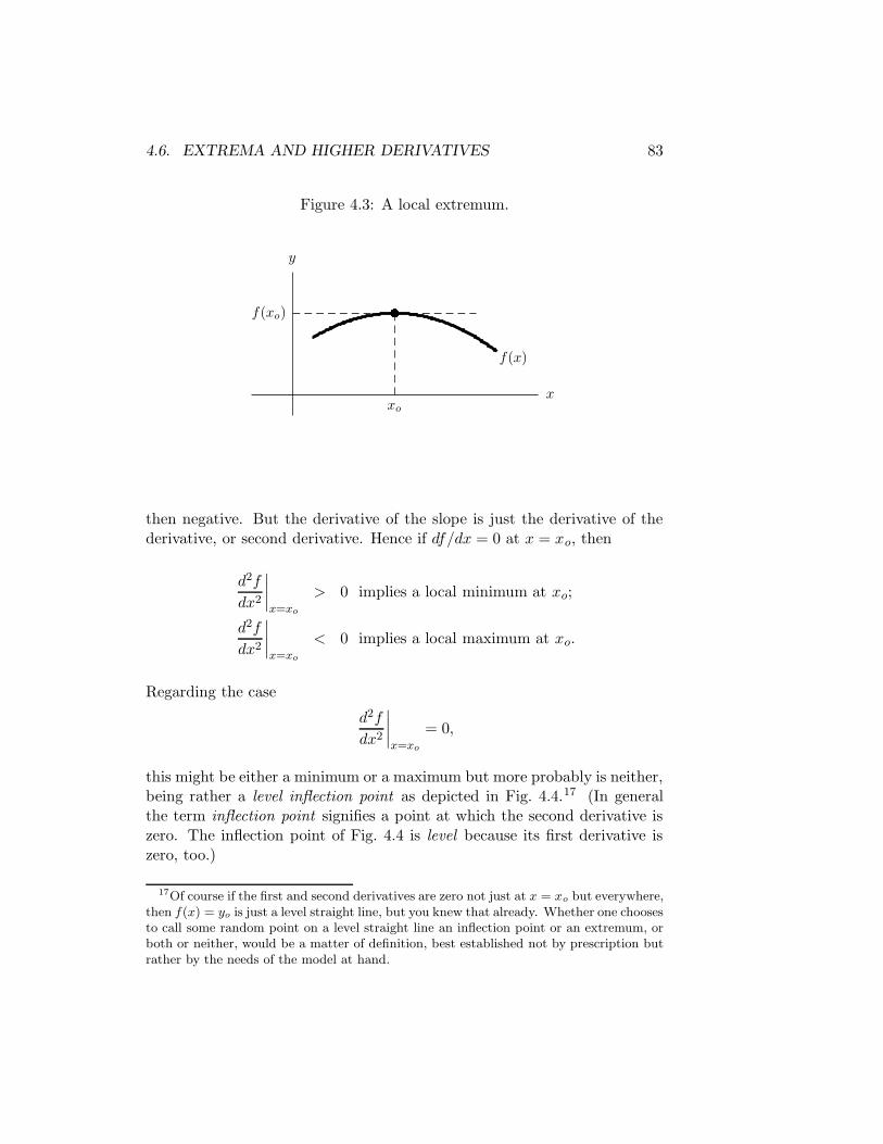
4.6. EXTREMA AND HIGHER DERIVATIVES 83
Figure 4.3: A local extremum.
xo
f(xo)
f(x)
x
y
then negative. But the derivative of the slope is just the derivative of thederivative, or second derivative. Hence if df/dx = 0 at x = xo, then
d2f
dx2
∣
∣
∣
∣
x=xo
> 0 implies a local minimum at xo;
d2f
dx2
∣
∣
∣
∣
x=xo
< 0 implies a local maximum at xo.
Regarding the case
d2f
dx2
∣
∣
∣
∣
x=xo
= 0,
this might be either a minimum or a maximum but more probably is neither,being rather a level inflection point as depicted in Fig. 4.4.17 (In generalthe term inflection point signifies a point at which the second derivative iszero. The inflection point of Fig. 4.4 is level because its first derivative iszero, too.)
17Of course if the first and second derivatives are zero not just at x = xo but everywhere,then f(x) = yo is just a level straight line, but you knew that already. Whether one choosesto call some random point on a level straight line an inflection point or an extremum, orboth or neither, would be a matter of definition, best established not by prescription butrather by the needs of the model at hand.

84 CHAPTER 4. THE DERIVATIVE
Figure 4.4: A level inflection.
xo
f(xo)
f(x)
x
y
4.7 L’Hopital’s rule
If z = zo is a root of both f(z) and g(z), or alternately if z = zo is a pole ofboth functions—that is, if both functions go to zero or infinity together atz = zo—then l’Hopital’s rule holds that
limz→zo
f(z)
g(z)=
df/dz
dg/dz
∣
∣
∣
∣
z=zo
. (4.29)
In the case where z = zo is a root, l’Hopital’s rule is proved by reasoning18
limz→zo
f(z)
g(z)= lim
z→zo
f(z)− 0
g(z) − 0
= limz→zo
f(z)− f(zo)
g(z)− g(zo)= lim
z→zo
df
dg= lim
z→zo
df/dz
dg/dz.
In the case where z = zo is a pole, new functions F (z) ≡ 1/f(z) andG(z) ≡ 1/g(z) of which z = zo is a root are defined, with which
limz→zo
f(z)
g(z)= lim
z→zo
G(z)
F (z)= lim
z→zo
dG
dF= lim
z→zo
−dg/g2
−df/f2,
where we have used the fact from (4.21) that d(1/u) = −du/u2 for any u.Canceling the minus signs and multiplying by g2/f2, we have that
limz→zo
g(z)
f(z)= lim
z→zo
dg
df.
18Partly with reference to [3, “L’Hopital’s rule,” 03:40, 5 April 2006].

4.8. THE NEWTON-RAPHSON ITERATION 85
Inverting,
limz→zo
f(z)
g(z)= lim
z→zo
df
dg= lim
z→zo
df/dz
dg/dz.
What about the case where zo is infinite? In this case, we define the newvariable Z = 1/z and the new functions Φ(Z) = f(1/Z) = f(z) and Γ(Z) =g(1/Z) = g(z), with which we can apply L’Hopital’s rule for Z → 0 to obtain
limz→zo
f(z)
g(z)= lim
Z→0
Φ(Z)
Γ(Z)= lim
Z→0
dΦ/dZ
dΓ/dZ= lim
Z→0
d[
f(
1Z
)]
/dZ
d[
g(
1Z
)]
/dZ
= limZ→0
(df/dz)(dz/dZ)
(dg/dz)(dz/dZ)= lim
z→zo
(df/dz)(−z2)
(dg/dz)(−z2)= lim
z→zo
df/dz
dg/dz.
Nothing in the derivation requires that z or zo be real.
L’Hopital’s rule is used in evaluating indeterminate forms of the kinds0/0 and∞/∞, plus related forms like (0)(∞) which can be recast into eitherof the two main forms. Good examples of the use require math from Ch. 5and later, but if we may borrow from (5.7) the natural logarithmic functionand its derivative,19
d
dxlnx =
1
x,
then a typical L’Hopital example is20
limx→∞
lnx√x
= limx→∞
1/x
1/2√x
= limx→∞
2√x
= 0.
This shows that natural logarithms grow slower than square roots.
Section 5.3 will put l’Hopital’s rule to work.
4.8 The Newton-Raphson iteration
The Newton-Raphson iteration is a powerful, fast converging, broadly appli-cable method for finding roots numerically. Given a function f(z) of whichthe root is desired, the Newton-Raphson iteration is
zk+1 = zk −f(z)ddzf(z)
∣
∣
∣
∣
∣
z=zk
. (4.30)
19This paragraph is optional reading for the moment. You can read Ch. 5 first, thencome back here and read the paragraph if you prefer.
20[33, § 10-2]

86 CHAPTER 4. THE DERIVATIVE
Figure 4.5: The Newton-Raphson iteration.
xk xk+1
f(x)
x
y
One begins the iteration by guessing the root and calling the guess z0.Then z1, z2, z3, etc., calculated in turn by the iteration (4.30), give suc-cessively better estimates of the true root z∞.
To understand the Newton-Raphson iteration, consider the function y =f(x) of Fig 4.5. The iteration approximates the curve f(x) by its tangentline21 (shown as the dashed line in the figure):
fk(x) = f(xk) +
[
d
dxf(x)
]
x=xk
(x− xk).
It then approximates the root xk+1 as the point at which fk(xk+1) = 0:
fk(xk+1) = 0 = f(xk) +
[
d
dxf(x)
]
x=xk
(xk+1 − xk).
Solving for xk+1, we have that
xk+1 = xk −f(x)ddxf(x)
∣
∣
∣
∣
∣
x=xk
,
which is (4.30) with x← z.
21A tangent line, also just called a tangent, is the line which most nearly approximatesa curve at a given point. The tangent touches the curve at the point, and in the neighbor-hood of the point it goes in the same direction the curve goes. The dashed line in Fig. 4.5is a good example of a tangent line.

4.8. THE NEWTON-RAPHSON ITERATION 87
Although the illustration uses real numbers, nothing forbids complex zand f(z). The Newton-Raphson iteration works just as well for these.
The principal limitation of the Newton-Raphson arises when the functionhas more than one root, as most interesting functions do. The iteration oftenbut not always converges on the root nearest the initial guess zo; but in anycase there is no guarantee that the root it finds is the one you wanted. Themost straightforward way to beat this problem is to find all the roots: firstyou find some root α, then you remove that root (without affecting any ofthe other roots) by dividing f(z)/(z − α), then you find the next root byiterating on the new function f(z)/(z − α), and so on until you have foundall the roots. If this procedure is not practical (perhaps because the functionhas a large or infinite number of roots), then you should probably take careto make a sufficiently accurate initial guess if you can.
A second limitation of the Newton-Raphson is that if one happens toguess z0 badly, the iteration may never converge on the root. For example,the roots of f(z) = z2 + 2 are z = ±i
√2, but if you guess that z0 = 1 then
the iteration has no way to leave the real number line, so it never converges.You fix this by setting z0 to a complex initial guess.
A third limitation arises where there is a multiple root. In this case,the Newton-Raphson normally still converges, but relatively slowly. Forinstance, the Newton-Raphson converges relatively slowly on the triple rootof f(z) = z3.
Usually in practice, the Newton-Raphson works very well. For mostfunctions, once the Newton-Raphson finds the root’s neighborhood, it con-verges on the actual root remarkably fast. Figure 4.5 shows why: in theneighborhood, the curve hardly departs from the straight line.
The Newton-Raphson iteration is a champion square root calculator,incidentally. Consider
f(x) = x2 − p,
whose roots are
x = ±√p.
Per (4.30), the Newton-Raphson iteration for this is
xk+1 =1
2
[
xk +p
xk
]
. (4.31)
If you start by guessing
x0 = 1

88 CHAPTER 4. THE DERIVATIVE
and iterate several times, the iteration (4.31) converges on x∞ =√p fast.
To calculate the nth root x = p1/n, let
f(x) = xn − p
and iterate22 ,23
xk+1 =1
n
[
(n− 1)xk +p
xn−1k
]
. (4.32)
Chapter 8 continues the general discussion of the derivative, treating theTaylor series.
22Equations (4.31) and (4.32) converge successfully toward x = p1/n for most com-plex p and x0. Given x0 = 1, however, they converge reliably and orderly only for real,nonnegative p. (To see why, sketch f(x) in the fashion of Fig. 4.5.)
If reliable, orderly convergence is needed for complex p = u + iv = σ cisψ, σ ≥ 0, youcan decompose p1/n per de Moivre’s theorem (3.26) as p1/n = σ1/n cis(ψ/n), in whichcis(ψ/n) = cos(ψ/n)+ i sin(ψ/n) is calculated by the Taylor series of Table 8.1. Then σ isreal and nonnegative, so (4.31) or (4.32) converges toward σ1/n in a reliable and orderlymanner.
The Newton-Raphson iteration however excels as a practical root-finding technique,so it often pays to be a little less theoretically rigid in applying it. When the iterationdoes not seem to converge, the best tactic may simply be to start over again with somerandomly chosen complex x0. This usually works, and it saves a lot of trouble.
23[33, § 4-9][29, § 6.1.1][39]

Chapter 5
The complex exponential
In higher mathematics, the complex exponential is almost impossible toavoid. It seems to appear just about everywhere. This chapter introducesthe concept of the natural exponential and of its inverse, the natural log-arithm; and shows how the two operate on complex arguments. It derivesthe functions’ basic properties and explains their close relationship to thetrigonometrics. It works out the functions’ derivatives and the derivativesof the basic members of the trigonometric and inverse trigonometric familiesto which they respectively belong.
5.1 The real exponential
Consider the factor(1 + ε)N .
This is the overall factor by which a quantity grows after N iterative roundsof multiplication by (1 + ε). What happens when ε is very small but N isvery large? The really interesting question is, what happens in the limit, asε → 0 and N → ∞, while x = εN remains a finite number? The answer isthat the factor becomes
expx ≡ limε→0+
(1 + ε)x/ε. (5.1)
Equation (5.1) is the definition of the exponential function or natural expo-nential function. We can alternately write the same definition in the form
expx = ex, (5.2)
e ≡ limε→0+
(1 + ε)1/ε. (5.3)
89

90 CHAPTER 5. THE COMPLEX EXPONENTIAL
Whichever form we write it in, the question remains as to whether thelimit actually exists; that is, whether 0 < e <∞; whether in fact we can putsome concrete bound on e. To show that we can,1 we observe per (4.15)2
that the derivative of the exponential function is
d
dxexpx = lim
δ→0+
exp(x+ δ/2) − exp(x− δ/2)δ
= limδ,ε→0+
(1 + ε)(x+δ/2)/ε − (1 + ε)(x−δ/2)/ε
δ
= limδ,ε→0+
(1 + ε)x/ε(1 + ε)+δ/2ε − (1 + ε)−δ/2ε
δ
= limδ,ε→0+
(1 + ε)x/ε(1 + δ/2) − (1− δ/2)
δ
= limε→0+
(1 + ε)x/ε,
which is to say thatd
dxexpx = expx. (5.4)
This is a curious, important result: the derivative of the exponential functionis the exponential function itself; the slope and height of the exponentialfunction are everywhere equal. For the moment, however, what interests usis that
d
dxexp 0 = exp 0 = lim
ε→0+(1 + ε)0 = 1,
which says that the slope and height of the exponential function are bothunity at x = 0, implying that the straight line which best approximatesthe exponential function in that neighborhood—the tangent line, which justgrazes the curve—is
y(x) = 1 + x.
With the tangent line y(x) found, the next step toward putting a concretebound on e is to show that y(x) ≤ expx for all real x, that the curve runsnowhere below the line. To show this, we observe per (5.1) that the essentialaction of the exponential function is to multiply repeatedly by 1 + ε as x
1Excepting (5.4), the author would prefer to omit much of the rest of this section, buteven at the applied level cannot think of a logically permissible way to do it. It seemsnonobvious that the limit limε→0+(1 + ε)1/ε actually does exist. The rest of this sectionshows why it does.
2Or per (4.19). It works the same either way.

5.1. THE REAL EXPONENTIAL 91
increases, to divide repeatedly by 1 + ε as x decreases. Since 1 + ε > 1, thisaction means for real x that
expx1 ≤ expx2 if x1 ≤ x2.
However, a positive number remains positive no matter how many times onemultiplies or divides it by 1 + ε, so the same action also means that
0 ≤ exp x
for all real x. In light of (5.4), the last two equations imply further that
d
dxexpx1 ≤ d
dxexpx2 if x1 ≤ x2,
0 ≤ d
dxexpx.
But we have purposely defined the line y(x) = 1 + x such that
exp 0 = y(0) = 1,
d
dxexp 0 =
d
dxy(0) = 1;
that is, such that the curve of expx just grazes the line y(x) at x = 0.Rightward, at x > 0, evidently the curve’s slope only increases, bendingupward away from the line. Leftward, at x < 0, evidently the curve’s slopeonly decreases, again bending upward away from the line. Either way, thecurve never crosses below the line for real x. In symbols,
y(x) ≤ expx.
Figure 5.1 depicts.Evaluating the last inequality at x = −1/2 and x = 1, we have that
1
2≤ exp
(
−1
2
)
,
2 ≤ exp (1) .
But per (5.2), expx = ex, so
1
2≤ e−1/2,
2 ≤ e1,

92 CHAPTER 5. THE COMPLEX EXPONENTIAL
Figure 5.1: The natural exponential.
x
expx
1
−1
or in other words,
2 ≤ e ≤ 4, (5.5)
which in consideration of (5.2) puts the desired bound on the exponentialfunction. The limit does exist.
By the Taylor series of Table 8.1, the value
e ≈ 0x2.B7E1
can readily be calculated, but the derivation of that series does not comeuntil Ch. 8.
5.2 The natural logarithm
In the general exponential expression ax, one can choose any base a; forexample, a = 2 is an interesting choice. As we shall see in § 5.4, however, itturns out that a = e, where e is the constant introduced in (5.3), is the mostinteresting choice of all. For this reason among others, the base-e logarithmis similarly interesting, such that we define for it the special notation
ln(·) = loge(·),
and call it the natural logarithm. Just as for any other base a, so also forbase a = e; thus the natural logarithm inverts the natural exponential andvice versa:
ln expx = ln ex = x,
exp lnx = eln x = x.(5.6)

5.2. THE NATURAL LOGARITHM 93
Figure 5.2: The natural logarithm.
x
lnx
−1
1
Figure 5.2 plots the natural logarithm.If
y = lnx,
thenx = exp y,
and per (5.4),dx
dy= exp y.
But this means thatdx
dy= x,
the inverse of which isdy
dx=
1
x.
In other words,d
dxlnx =
1
x. (5.7)
Like many of the equations in these early chapters, here is another rathersignificant result.3
3Besides the result itself, the technique which leads to the result is also interesting andis worth mastering. We shall use the technique more than once in this book.

94 CHAPTER 5. THE COMPLEX EXPONENTIAL
5.3 Fast and slow functions
The exponential expx is a fast function. The logarithm lnx is a slow func-tion. These functions grow, diverge or decay respectively faster and slowerthan xa.
Such claims are proved by l’Hopital’s rule (4.29). Applying the rule, wehave that
limx→∞
lnx
xa= lim
x→∞−1
axa=
0 if a > 0,
+∞ if a ≤ 0,
limx→0+
lnx
xa= lim
x→0+
−1
axa=
−∞ if a ≥ 0,
0 if a < 0,
(5.8)
which reveals the logarithm to be a slow function. Since the exp(·) and ln(·)functions are mutual inverses, we can leverage (5.8) to show also that
limx→∞
exp(±x)xa
= limx→∞
exp
[
lnexp(±x)
xa
]
= limx→∞
exp [±x− a lnx]
= limx→∞
exp
[
(x)
(
±1− a lnx
x
)]
= limx→∞
exp [(x) (±1− 0)]
= limx→∞
exp [±x] .
That is,
limx→∞
exp(+x)
xa=∞,
limx→∞
exp(−x)xa
= 0,
(5.9)
which reveals the exponential to be a fast function. Exponentials grow ordecay faster than powers; logarithms diverge slower.
Such conclusions are extended to bases other than the natural base esimply by observing that logb x = lnx/ ln b and that bx = exp(x ln b). Thusexponentials generally are fast and logarithms generally are slow, regardlessof the base.4
4There are of course some degenerate edge cases like a = 0 and b = 1. The reader candetail these as the need arises.

5.3. FAST AND SLOW FUNCTIONS 95
It is interesting and worthwhile to contrast the sequence
. . . ,− 3!
x4,2!
x3,− 1!
x2,0!
x1,x0
0!,x1
1!,x2
2!,x3
3!,x4
4!, . . .
against the sequence
. . . ,− 3!
x4,2!
x3,− 1!
x2,
0!
x1, lnx,
x1
1!,x2
2!,x3
3!,x4
4!, . . .
As x → +∞, each sequence increases in magnitude going rightward. Also,each term in each sequence is the derivative with respect to x of the term toits right—except left of the middle element in the first sequence and right ofthe middle element in the second. The exception is peculiar. What is goingon here?
The answer is that x0 (which is just a constant) and lnx both are ofzeroth order in x. This seems strange at first because lnx diverges as x→∞whereas x0 does not, but the divergence of the former is extremely slow—so slow, in fact, that per (5.8) limx→∞(lnx)/xε = 0 for any positive ε nomatter how small. Figure 5.2 has plotted lnx only for x ∼ 1, but beyond thefigure’s window the curve (whose slope is 1/x) flattens rapidly rightward, tothe extent that it locally resembles the plot of a constant value; and indeedone can write
x0 = limu→∞
ln(x+ u)
lnu,
which casts x0 as a logarithm shifted and scaled. Admittedly, one oughtnot strain such logic too far, because lnx is not in fact a constant, but thepoint nevertheless remains that x0 and lnx often play analogous roles inmathematics. The logarithm can in some situations profitably be thoughtof as a “diverging constant” of sorts.
Less strange-seeming perhaps is the consequence of (5.9) that expx is ofinfinite order in x, that x∞ and expx play analogous roles.
It befits an applied mathematician subjectively to internalize (5.8) and(5.9), to remember that lnx resembles x0 and that expx resembles x∞. Aqualitative sense that logarithms are slow and exponentials, fast, helps oneto grasp mentally the essential features of many mathematical models oneencounters in practice.
Now leaving aside fast and slow functions for the moment, we turn ourattention in the next section to the highly important matter of the expo-nential of a complex argument.

96 CHAPTER 5. THE COMPLEX EXPONENTIAL
5.4 Euler’s formula
The result of § 5.1 leads to one of the central questions in all of mathematics.How can one evaluate
exp iθ = limε→0+
(1 + ε)iθ/ε,
where i2 = −1 is the imaginary unit introduced in § 2.12?
To begin, one can take advantage of (4.14) to write the last equation inthe form
exp iθ = limε→0+
(1 + iε)θ/ε,
but from here it is not obvious where to go. The book’s development upto the present point gives no obvious direction. In fact it appears that theinterpretation of exp iθ remains for us to define, if we can find a way to defineit which fits sensibly with our existing notions of the real exponential. So,if we don’t quite know where to go with this yet, what do we know?
One thing we know is that if θ = ε, then
exp(iε) = (1 + iε)ε/ε = 1 + iε.
But per § 5.1, the essential operation of the exponential function is to multi-ply repeatedly by some factor, where the factor is not quite exactly unity—inthis case, by 1 + iε. So let us multiply a complex number z = x + iy by1 + iε, obtaining
(1 + iε)(x+ iy) = (x− εy) + i(y + εx).
The resulting change in z is
∆z = (1 + iε)(x+ iy)− (x+ iy) = (ε)(−y + ix),
in which it is seen that
|∆z| = (ε)√
y2 + x2 = (ε) |z| ;
arg(∆z) = arctanx
−y = arg z +2π
4.
In other words, the change is proportional to the magnitude of z, but at aright angle to z’s arm in the complex plane. Refer to Fig. 5.3.

5.4. EULER’S FORMULA 97
Figure 5.3: The complex exponential and Euler’s formula.
−i2
−i
i
i2
−2 −1 1 2
z
∆z
φρ
<(z)
i=(z)
Since the change is directed neither inward nor outward from the dashedcircle in the figure, evidently its effect is to move z a distance (ε) |z| coun-terclockwise about the circle. In other words, referring to the figure, thechange ∆z leads to
∆ρ = 0,
∆φ = ε.
These two equations—implying an unvarying, steady counterclockwise pro-gression about the circle in the diagram—are somewhat unexpected. Giventhe steadiness of the progression, it follows from the equations that
|exp iθ| = limε→0+
∣
∣
∣(1 + iε)θ/ε
∣
∣
∣= |exp 0|+ lim
ε→0+
θ
ε∆ρ = 1;
arg [exp iθ] = limε→0+
arg[
(1 + iε)θ/ε]
= arg [exp 0] + limε→0+
θ
ε∆φ = θ.
That is, exp iθ is the complex number which lies on the Argand unit circleat phase angle θ. In terms of sines and cosines of θ, such a number can bewritten
exp iθ = cos θ + i sin θ = cis θ, (5.10)
where cis(·) is as defined in § 3.11. Or, since φ ≡ arg(exp iθ) = θ,
exp iφ = cosφ+ i sinφ = cisφ. (5.11)

98 CHAPTER 5. THE COMPLEX EXPONENTIAL
Along with the Pythagorean theorem (2.47), the fundamental theoremof calculus (7.2) and Cauchy’s integral formula (8.28), (5.11) is perhaps oneof the four most famous results in all of mathematics. It is called Euler’sformula,5 ,6 and it opens the exponential domain fully to complex numbers,not just for the natural base e but for any base. To see this, consider inlight of Fig. 5.3 and (5.11) that one can express any complex number in theform
z = x+ iy = ρ exp iφ.
If a complex base w is similarly expressed in the form
w = u+ iv = σ exp iψ,
then it follows that
wz = exp[lnwz]
= exp[z lnw]
= exp[(x+ iy)(iψ + lnσ)]
= exp[(x lnσ − ψy) + i(y lnσ + ψx)].
Since exp(α+ β) = eα+β = expα expβ, the last equation is
wz = exp(x lnσ − ψy) exp i(y lnσ + ψx), (5.12)
where
x = ρ cosφ,
y = ρ sinφ,
σ =√
u2 + v2,
tanψ =v
u.
Equation (5.12) serves to raise any complex number to a complex power.
5For native English speakers who do not speak German, Leonhard Euler’s name ispronounced as “oiler.”
6An alternate derivation of Euler’s formula (5.11)—less intuitive and requiring slightlymore advanced mathematics, but briefer—constructs from Table 8.1 the Taylor seriesfor exp iφ, cos φ and i sinφ, then adds the latter two to show them equal to the firstof the three. Such an alternate derivation lends little insight, perhaps, but at least itbuilds confidence that we actually knew what we were doing when we came up with theincredible (5.11).

5.5. COMPLEX EXPONENTIALS AND DE MOIVRE 99
Curious consequences of Euler’s formula (5.11) include that
e±i2π/4 = ±i,e±i2π/2 = −1,
ein2π = 1.
(5.13)
For the natural logarithm of a complex number in light of Euler’s formula,we have that
lnw = ln(
σeiψ)
= lnσ + iψ. (5.14)
5.5 Complex exponentials and de Moivre’s theo-rem
Euler’s formula (5.11) implies that complex numbers z1 and z2 can be written
z1 = ρ1eiφ1 ,
z2 = ρ2eiφ2 .
(5.15)
By the basic power properties of Table 2.2, then,
z1z2 = ρ1ρ2ei(φ1+φ2) = ρ1ρ2 exp[i(φ1 + φ2)],
z1z2
=ρ1
ρ2ei(φ1−φ2) =
ρ1
ρ2exp[i(φ1 − φ2)],
za = ρaeiaφ = ρa exp[iaφ].
(5.16)
This is de Moivre’s theorem, introduced in § 3.11.
5.6 Complex trigonometrics
Applying Euler’s formula (5.11) to +φ then to −φ, we have that
exp(+iφ) = cosφ+ i sinφ,
exp(−iφ) = cosφ− i sinφ.
Adding the two equations and solving for cosφ yields
cosφ =exp(+iφ) + exp(−iφ)
2. (5.17)

100 CHAPTER 5. THE COMPLEX EXPONENTIAL
Subtracting the second equation from the first and solving for sinφ yields
sinφ =exp(+iφ)− exp(−iφ)
i2. (5.18)
Thus are the trigonometrics expressed in terms of complex exponentials.The forms (5.17) and (5.18) suggest the definition of new functions
coshφ ≡ exp(+φ) + exp(−φ)
2, (5.19)
sinhφ ≡ exp(+φ)− exp(−φ)
2, (5.20)
tanhφ ≡ sinhφ
coshφ. (5.21)
These are called the hyperbolic functions. Their inverses arccosh, etc., are de-fined in the obvious way. The Pythagorean theorem for trigonometrics (3.2)is that cos2 φ + sin2 φ = 1; and from (5.19) and (5.20) one can derive thehyperbolic analog:
cos2 φ+ sin2 φ = 1,
cosh2 φ− sinh2 φ = 1.(5.22)
The notation exp i(·) or ei(·) is sometimes felt to be too bulky. Althoughless commonly seen than the other two, the notation
cis(·) ≡ exp i(·) = cos(·) + i sin(·)
is also conventionally recognized, as earlier seen in § 3.11. Also conven-tionally recognized are sin−1(·) and occasionally asin(·) for arcsin(·), andlikewise for the several other trigs.
Replacing z ← φ in this section’s several equations implies a coherentdefinition for trigonometric functions of a complex variable. Then, compar-ing (5.17) and (5.18) respectively to (5.19) and (5.20), we have that
cosh z = cos iz,
i sinh z = sin iz,
i tanh z = tan iz,
(5.23)
by which one can immediately adapt the many trigonometric properties ofTables 3.1 and 3.3 to hyperbolic use.
At this point in the development one begins to notice that the sin, cos,exp, cis, cosh and sinh functions are each really just different facets of the

5.7. SUMMARY OF PROPERTIES 101
same mathematical phenomenon. Likewise their respective inverses: arcsin,arccos, ln, −i ln, arccosh and arcsinh. Conventional names for these twomutually inverse families of functions are unknown to the author, but onemight call them the natural exponential and natural logarithmic families.If the various tangent functions were included, one might call them thetrigonometric and inverse trigonometric families.
5.7 Summary of properties
Table 5.1 gathers properties of the complex exponential from this chapterand from §§ 2.12, 3.11 and 4.4.
5.8 Derivatives of complex exponentials
This section computes the derivatives of the various trigonometric and in-verse trigonometric functions.
5.8.1 Derivatives of sine and cosine
One can indeed compute derivatives of the sine and cosine functions from(5.17) and (5.18), but to do it in that way doesn’t seem sporting. Betterapplied style is to find the derivatives by observing directly the circle fromwhich the sine and cosine functions come. Refer to Fig. 5.4. Suppose thatthe point z in the figure is not fixed but is traveling steadily about the circlesuch that
z(t) = (ρ) [cos(ωt+ φo) + i sin(ωt+ φo)] . (5.24)
How fast then is the rate dz/dt, and in what Argand direction?
dz
dt= (ρ)
[
d
dtcos(ωt+ φo) + i
d
dtsin(ωt+ φo)
]
. (5.25)
Evidently,
• the speed is |dz/dt| = (ρ)(dφ/dt) = ρω;
• the direction is at right angles to the arm of ρ, which is to say thatarg(dz/dt) = φ+ 2π/4.
With these observations we can write that
dz
dt= (ρω)
[
cos
(
ωt+ φo +2π
4
)
+ i sin
(
ωt+ φo +2π
4
)]
= (ρω) [− sin(ωt+ φo) + i cos(ωt+ φo)] . (5.26)

102 CHAPTER 5. THE COMPLEX EXPONENTIAL
Table 5.1: Complex exponential properties.
i2 = −1 = (−i)21
i= −i
eiφ = cosφ+ i sinφ
eiz = cos z + i sin z
z1z2 = ρ1ρ2ei(φ1+φ2) = (x1x2 − y1y2) + i(y1x2 + x1y2)
z1z2
=ρ1
ρ2ei(φ1−φ2) =
(x1x2 + y1y2) + i(y1x2 − x1y2)
x22 + y2
2
za = ρaeiaφ
wz = ex ln σ−ψyei(y lnσ+ψx)
lnw = lnσ + iψ
sin z =eiz − e−iz
i2sin iz = i sinh z sinh z =
ez − e−z2
cos z =eiz + e−iz
2cos iz = cosh z cosh z =
ez + e−z
2
tan z =sin z
cos ztan iz = i tanh z tanh z =
sinh z
cosh z
cos2 z + sin2 z = 1 = cosh2 z − sinh2 z
z ≡ x+ iy = ρeiφ
w ≡ u+ iv = σeiψ
exp z ≡ ez
cis z ≡ cos z + i sin z = eiz
d
dzexp z = exp z
d
dwlnw =
1
wdf/dz
f(z)=
d
dzln f(z)

5.8. DERIVATIVES OF COMPLEX EXPONENTIALS 103
Figure 5.4: The derivatives of the sine and cosine functions.
z
dz
dt
ωt+ φo
ρ
<(z)
=(z)
Matching the real and imaginary parts of (5.25) against those of (5.26), wehave that
d
dtcos(ωt+ φo) = −ω sin(ωt+ φo),
d
dtsin(ωt+ φo) = +ω cos(ωt+ φo).
(5.27)
If ω = 1 and φo = 0, these are
d
dtcos t = − sin t,
d
dtsin t = +cos t.
(5.28)
5.8.2 Derivatives of the trigonometrics
The derivatives of exp(·), sin(·) and cos(·), eqns. (5.4) and (5.28) give. Fromthese, with the help of (5.22) and of the derivative chain and product rules(§ 4.5), we can calculate the derivatives in Table 5.2.7
7[33, back endpaper]

104 CHAPTER 5. THE COMPLEX EXPONENTIAL
Table 5.2: Derivatives of the trigonometrics.
d
dzexp z = +exp z
d
dz
1
exp z= − 1
exp z
d
dzsin z = +cos z
d
dz
1
sin z= − 1
tan z sin zd
dzcos z = − sin z
d
dz
1
cos z= +
tan z
cos z
d
dztan z = +
(
1 + tan2 z)
= +1
cos2 zd
dz
1
tan z= −
(
1 +1
tan2 z
)
= − 1
sin2 z
d
dzsinh z = +cosh z
d
dz
1
sinh z= − 1
tanh z sinh zd
dzcosh z = +sinh z
d
dz
1
cosh z= −tanh z
cosh z
d
dztanh z = 1− tanh2 z = +
1
cosh2 zd
dz
1
tanh z= 1− 1
tanh2 z= − 1
sinh2 z

5.8. DERIVATIVES OF COMPLEX EXPONENTIALS 105
5.8.3 Derivatives of the inverse trigonometrics
Observe the pair
d
dzexp z = exp z,
d
dwlnw =
1
w.
The natural exponential exp z belongs to the trigonometric family of func-tions, as does its derivative. The natural logarithm lnw, by contrast, belongsto the inverse trigonometric family of functions, but its derivative is simpler,not a trigonometric or inverse trigonometric function at all. In Table 5.2,one notices that all the trigonometrics have trigonometric derivatives. Byanalogy with the natural logarithm, do all the inverse trigonometrics havesimpler derivatives?
It turns out that they do. Refer to the account of the natural logarithm’sderivative in § 5.2. Following a similar procedure, we have by successive stepsthat
arcsinw = z,
w = sin z,
dw
dz= cos z,
dw
dz= ±
√
1− sin2 z,
dw
dz= ±
√
1− w2,
dz
dw=
±1√1− w2
,
d
dwarcsinw =
±1√1− w2
. (5.29)

106 CHAPTER 5. THE COMPLEX EXPONENTIAL
Table 5.3: Derivatives of the inverse trigonometrics.
d
dwlnw =
1
wd
dwarcsinw =
±1√1− w2
d
dwarccosw =
∓1√1− w2
d
dwarctanw =
1
1 + w2
d
dwarcsinhw =
±1√w2 + 1
d
dwarccoshw =
±1√w2 − 1
d
dwarctanhw =
1
1− w2
Similarly,
arctanw = z,
w = tan z,
dw
dz= 1 + tan2 z,
dw
dz= 1 + w2,
dz
dw=
1
1 + w2,
d
dwarctanw =
1
1 + w2. (5.30)
Derivatives of the other inverse trigonometrics are found in the same way.Table 5.3 summarizes.
5.9 The actuality of complex quantities
Doing all this neat complex math, the applied mathematician can lose sightof some questions he probably ought to keep in mind: Is there really such a

5.9. THE ACTUALITY OF COMPLEX QUANTITIES 107
thing as a complex quantity in nature? If not, then hadn’t we better avoidthese complex quantities, leaving them to the professional mathematicaltheorists?
As developed by Oliver Heaviside in 1887,8 the answer depends on yourpoint of view. If I have 300 g of grapes and 100 g of grapes, then I have 400 galtogether. Alternately, if I have 500 g of grapes and −100 g of grapes,again I have 400 g altogether. (What does it mean to have −100 g ofgrapes? Maybe I ate some.) But what if I have 200 + i100 g of grapesand 200− i100 g of grapes? Answer: again, 400 g.
Probably you would not choose to think of 200 + i100 g of grapesand 200 − i100 g of grapes, but because of (5.17) and (5.18), one oftendescribes wave phenomena as linear superpositions (sums) of countervailingcomplex exponentials. Consider for instance the propagating wave
A cos[ωt− kz] =A
2exp[+i(ωt− kz)] +
A
2exp[−i(ωt− kz)].
The benefit of splitting the real cosine into two complex parts is that whilethe magnitude of the cosine changes with time t, the magnitude of eitherexponential alone remains steady (see the circle in Fig. 5.3). It turns out tobe much easier to analyze two complex wave quantities of constant magni-tude than to analyze one real wave quantity of varying magnitude. Betteryet, since each complex wave quantity is the complex conjugate of the other,the analyses thereof are mutually conjugate, too; so you normally needn’tactually analyze the second. The one analysis suffices for both.9 (It’s likereflecting your sister’s handwriting. To read her handwriting backward, youneedn’t ask her to try writing reverse with the wrong hand; you can justhold her regular script up to a mirror. Of course, this ignores the question ofwhy one would want to reflect someone’s handwriting in the first place; butanyway, reflecting—which is to say, conjugating—complex quantities oftenis useful.)
Some authors have gently denigrated the use of imaginary parts in phys-ical applications as a mere mathematical trick, as though the parts were notactually there. Well, that is one way to treat the matter, but it is not theway this book recommends. Nothing in the mathematics requires you to
8[2]9If the point is not immediately clear, an example: Suppose that by the Newton-
Raphson iteration (§ 4.8) you have found a root of the polynomial x3 + 2x2 + 3x + 4 atx ≈ −0x0.2D+ i0x1.8C. Where is there another root? Answer: at the complex conjugate,x ≈ −0x0.2D − i0x1.8C. One need not actually run the Newton-Raphson again to findthe conjugate root.

108 CHAPTER 5. THE COMPLEX EXPONENTIAL
regard the imaginary parts as physically nonexistent. You need not abuseOccam’s razor! It is true by Euler’s formula (5.11) that a complex exponen-tial exp iφ can be decomposed into a sum of trigonometrics. However, it isequally true by the complex trigonometric formulas (5.17) and (5.18) that atrigonometric can be decomposed into a sum of complex exponentials. So, ifeach can be decomposed into the other, then which of the two is the real de-composition? Answer: it depends on your point of view. Experience seemsto recommend viewing the complex exponential as the basic element—as theelement of which the trigonometrics are composed—rather than the otherway around. From this point of view, it is (5.17) and (5.18) which are thereal decomposition. Euler’s formula itself is secondary.
The complex exponential method of offsetting imaginary parts offers anelegant yet practical mathematical way to model physical wave phenomena.So go ahead: regard the imaginary parts as actual. It doesn’t hurt anything,and it helps with the math.

Chapter 6
Primes, roots and averages
This chapter gathers a few significant topics, each of whose treatment seemstoo brief for a chapter of its own.
6.1 Prime numbers
A prime number—or simply, a prime—is an integer greater than one, divis-ible only by one and itself. A composite number is an integer greater thanone and not prime. A composite number can be composed as a product oftwo or more prime numbers. All positive integers greater than one are eithercomposite or prime.
The mathematical study of prime numbers and their incidents consti-tutes number theory, and it is a deep area of mathematics. The deeperresults of number theory seldom arise in applications,1 however, so we shallconfine our study of number theory in this book to one or two of its simplest,most broadly interesting results.
6.1.1 The infinite supply of primes
The first primes are evidently 2, 3, 5, 7, 0xB, . . . . Is there a last prime? Toshow that there is not, suppose that there were. More precisely, supposethat there existed exactly N primes, with N finite, letting p1, p2, . . . , pNrepresent these primes from least to greatest. Now consider the product of
1The deeper results of number theory do arise in cryptography, or so the author hasbeen led to understand. Although cryptography is literally an application of mathematics,its spirit is that of pure mathematics rather than of applied. If you seek cryptographicderivations, this book is probably not the one you want.
109

110 CHAPTER 6. PRIMES, ROOTS AND AVERAGES
all the primes,
C =
N∏
j=1
pj.
What of C + 1? Since p1 = 2 divides C, it cannot divide C + 1. Similarly,since p2 = 3 divides C, it also cannot divide C + 1. The same goes forp3 = 5, p4 = 7, p5 = 0xB, etc. Apparently none of the primes in the pjseries divides C + 1, which implies either that C + 1 itself is prime, or thatC + 1 is composed of primes not in the series. But the latter is assumedimpossible on the ground that the pj series includes all primes; and theformer is assumed impossible on the ground that C + 1 > C > pN , with pNthe greatest prime. The contradiction proves false the assumption whichgave rise to it. The false assumption: that there were a last prime.
Thus there is no last prime. No matter how great a prime number onefinds, a greater can always be found. The supply of primes is infinite.2
Attributed to the ancient geometer Euclid, the foregoing proof is a clas-sic example of mathematical reductio ad absurdum, or as usually styled inEnglish, proof by contradiction.3
6.1.2 Compositional uniqueness
Occasionally in mathematics, plausible assumptions can hide subtle logicalflaws. One such plausible assumption is the assumption that every positiveinteger has a unique prime factorization. It is readily seen that the firstseveral positive integers—1 = (), 2 = (21), 3 = (31), 4 = (22), 5 = (51),6 = (21)(31), 7 = (71), 8 = (23), . . .—each have unique prime factorizations,but is this necessarily true of all positive integers?
To show that it is true, suppose that it were not.4 More precisely, sup-pose that there did exist positive integers factorable each in two or moredistinct ways, with the symbol C representing the least such integer. Notingthat C must be composite (prime numbers by definition are each factorable
2[36]3[31, Appendix 1][3, “Reductio ad absurdum,” 02:36, 28 April 2006]4Unfortunately the author knows no more elegant proof than this, yet cannot even cite
this one properly. The author encountered the proof in some book over a decade ago. Theidentity of that book is now long forgotten.

6.1. PRIME NUMBERS 111
only one way, like 5 = [51]), let
Cp ≡Np∏
j=1
pj,
Cq ≡Nq∏
k=1
qk,
Cp = Cq = C,
pj ≤ pj+1,
qk ≤ qk+1,
p1 ≤ q1,
Np > 1,
Nq > 1,
where Cp and Cq represent two distinct prime factorizations of the samenumber C and where the pj and qk are the respective primes ordered fromleast to greatest. We see that
pj 6= qk
for any j and k—that is, that the same prime cannot appear in bothfactorizations—because if the same prime r did appear in both then C/rwould constitute an ambiguously factorable positive integer less than C,when we had already defined C to represent the least such. Among othereffects, the fact that pj 6= qk strengthens the definition p1 ≤ q1 to read
p1 < q1.
Let us now rewrite the two factorizations in the form
Cp = p1Ap,
Cq = q1Aq,
Cp = Cq = C,
Ap ≡Np∏
j=2
pj ,
Aq ≡Nq∏
k=2
qk,
112 CHAPTER 6. PRIMES, ROOTS AND AVERAGES
where p1 and q1 are the least primes in their respective factorizations.Since C is composite and since p1 < q1, we have that
1 < p1 < q1 ≤√C ≤ Aq < Ap < C,
which implies that
p1q1 < C.
The last inequality lets us compose the new positive integer
B = C − p1q1,
which might be prime or composite (or unity), but which either way enjoysa unique prime factorization because B < C, with C the least positiveinteger factorable two ways. Observing that some integer s which divides Cnecessarily also divides C ± ns, we note that each of p1 and q1 necessarilydivides B. This means that B’s unique factorization includes both p1 and q1,which further means that the product p1q1 divides B. But if p1q1 divides B,then it divides B + p1q1 = C, also.
Let E represent the positive integer which results from dividing Cby p1q1:
E ≡ C
p1q1.
Then,
Eq1 =C
p1= Ap,
Ep1 =C
q1= Aq.
That Eq1 = Ap says that q1 divides Ap. But Ap < C, so Ap’s primefactorization is unique—and we see above that Ap’s factorization does notinclude any qk, not even q1. The contradiction proves false the assumptionwhich gave rise to it. The false assumption: that there existed a leastcomposite number C prime-factorable in two distinct ways.
Thus no positive integer is ambiguously factorable. Prime factorizationsare always unique.
We have observed at the start of this subsection that plausible assump-tions can hide subtle logical flaws. Indeed this is so. Interestingly however,the plausible assumption of the present subsection has turned out absolutelycorrect; we have just had to do some extra work to prove it. Such effects

6.1. PRIME NUMBERS 113
are typical on the shadowed frontier where applied shades into pure math-ematics: with sufficient experience and with a firm grasp of the model athand, if you think that it’s true, then it probably is. Judging when to delveinto the mathematics anyway, seeking a more rigorous demonstration of aproposition one feels pretty sure is correct, is a matter of applied mathe-matical style. It depends on how sure one feels, and more importantly onwhether the unsureness felt is true uncertainty or is just an unaccountabledesire for more precise mathematical definition (if the latter, then unlikethe author you may have the right temperament to become a professionalmathematician). The author does judge the present subsection’s proof tobe worth the applied effort; but nevertheless, when one lets logical minutiaedistract him to too great a degree, he admittedly begins to drift out of theapplied mathematical realm that is the subject of this book.
6.1.3 Rational and irrational numbers
A rational number is a finite real number expressible as a ratio of integers
x =p
q, q 6= 0.
The ratio is fully reduced if p and q have no prime factors in common. Forinstance, 4/6 is not fully reduced, whereas 2/3 is.
An irrational number is a finite real number which is not rational. Forexample,
√2 is irrational. In fact any x =
√n is irrational unless integral;
there is no such thing as a√n which is not an integer but is rational.
To prove5 the last point, suppose that there did exist a fully reduced
x =p
q=√n, p > 0, q > 1,
where p, q and n are all integers. Squaring the equation, we have that
p2
q2= n,
which form is evidently also fully reduced. But if q > 1, then the fullyreduced n = p2/q2 is not an integer as we had assumed that it was. Thecontradiction proves false the assumption which gave rise to it. Hence thereexists no rational, nonintegral
√n, as was to be demonstrated. The proof is
readily extended to show that any x = nj/k is irrational if nonintegral, the
5A proof somewhat like the one presented here is found in [31, Appendix 1].

114 CHAPTER 6. PRIMES, ROOTS AND AVERAGES
extension by writing pk/qk = nj then following similar steps as those thisparagraph outlines.
That’s all the number theory the book treats; but in applied math, solittle will take you pretty far. Now onward we go to other topics.
6.2 The existence and number of polynomial roots
This section shows that anNth-order polynomial must have exactly N roots.
6.2.1 Polynomial roots
Consider the quotient B(z)/A(z), where
A(z) = z − α,
B(z) =N∑
k=0
bkzk, N > 0, bN 6= 0,
B(α) = 0.
In the long-division symbology of Table 2.3,
B(z) = A(z)Q0(z) +R0(z),
where Q0(z) is the quotient and R0(z), a remainder. In this case the divisorA(z) = z−α has first order, and as § 2.6.2 has observed, first-order divisorsleave zeroth-order, constant remainders R0(z) = ρ. Thus substituting leaves
B(z) = (z − α)Q0(z) + ρ.
When z = α, this reduces to
B(α) = ρ.
But B(α) = 0, soρ = 0.
Evidently the division leaves no remainder ρ, which is to say that z − αexactly divides every polynomial B(z) of which z = α is a root.
Note that if the polynomial B(z) has order N , then the quotient Q(z) =B(z)/(z − α) has exactly order N − 1. That is, the leading, zN−1 term ofthe quotient is never null. The reason is that if the leading term were null, ifQ(z) had order less than N −1, then B(z) = (z−α)Q(z) could not possiblyhave order N as we have assumed.

6.2. THE EXISTENCE AND NUMBER OF ROOTS 115
6.2.2 The fundamental theorem of algebra
The fundamental theorem of algebra holds that any polynomial B(z) of or-der N can be factored
B(z) =N∑
k=0
bkzk = bN
N∏
j=1
(z − αj), bN 6= 0, (6.1)
where the αk are the N roots of the polynomial.6
To prove the theorem, it suffices to show that all polynomials of orderN > 0 have at least one root; for if a polynomial of order N has a root αN ,then according to § 6.2.1 one can divide the polynomial by z−αN to obtaina new polynomial of order N − 1. To the new polynomial the same logicapplies; if it has at least one root αN−1, then one can divide by z−αN−1 toobtain yet another polynomial of order N −2; and so on, one root extractedat each step, factoring the polynomial step by step into the desired formbN∏Nj=1(z − αj).
It remains however to show that there exists no polynomial B(z) of orderN > 0 lacking roots altogether. To show that there is no such polynomial,consider the locus7 of all B(ρeiφ) in the Argand range plane (Fig. 2.5), wherez = ρeiφ, ρ is held constant, and φ is variable. Because ei(φ+n2π) = eiφ andno fractional powers of z appear in (6.1), this locus forms a closed loop. Atvery large ρ, the bNz
N term dominates B(z), so the locus there evidentlyhas the general character of bNρ
NeiNφ. As such, the locus is nearly but notquite a circle at radius bNρ
N from the Argand origin B(z) = 0, revolving Ntimes at that great distance before exactly repeating. On the other hand,when ρ = 0 the entire locus collapses on the single point B(0) = b0.
Now consider the locus at very large ρ again, but this time let ρ slowlyshrink. Watch the locus as ρ shrinks. The locus is like a great string orrubber band, joined at the ends and looped in N great loops. As ρ shrinkssmoothly, the string’s shape changes smoothly. Eventually ρ disappears andthe entire string collapses on the point B(0) = b0. Since the string originallyhas looped N times at great distance about the Argand origin, but at theend has collapsed on a single point, then at some time between it must haveswept through the origin and every other point within the original loops.
6Professional mathematicians typically state the theorem in a slightly different form.They also prove it in rather a different way. [21, Ch. 10, Prob. 74]
7A locus is the geometric collection of points which satisfy a given criterion. Forexample, the locus of all points in a plane at distance ρ from a point O is a circle; thelocus of all points in three-dimensional space equidistant from two points P and Q is aplane; etc.

116 CHAPTER 6. PRIMES, ROOTS AND AVERAGES
After all, B(z) is everywhere differentiable, so the string can only sweepas ρ decreases; it can never skip. The Argand origin lies inside the loops atthe start but outside at the end. If so, then the values of ρ and φ preciselywhere the string has swept through the origin by definition constitute aroot B(ρeiφ) = 0. Thus as we were required to show, B(z) does have atleast one root, which observation completes the applied demonstration ofthe fundamental theorem of algebra.
The fact that the roots exist is one thing. Actually finding the roots nu-merically is another matter. For a quadratic (second order) polynomial, (2.2)gives the roots. For cubic (third order) and quartic (fourth order) polyno-mials, formulas for the roots are known (see Ch. 10) though seemingly notso for quintic (fifth order) and higher-order polynomials;8 but the Newton-Raphson iteration (§ 4.8) can be used to locate a root numerically in anycase. The Newton-Raphson is used to extract one root (any root) at eachstep as described above, reducing the polynomial step by step until all theroots are found.
The reverse problem, finding the polynomial given the roots, is mucheasier: one just multiplies out
∏
j(z − αj), as in (6.1).
6.3 Addition and averages
This section discusses the two basic ways to add numbers and the threebasic ways to calculate averages of them.
6.3.1 Serial and parallel addition
Consider the following problem. There are three masons. The strongestand most experienced of the three, Adam, lays 120 bricks per hour.9 Nextis Brian who lays 90. Charles is new; he lays only 60. Given eight hours,how many bricks can the three men lay? Answer:
(8 hours)(120 + 90 + 60 bricks per hour) = 2160 bricks.
Now suppose that we are told that Adam can lay a brick every 30 seconds;Brian, every 40 seconds; Charles, every 60 seconds. How much time do the
8In a celebrated theorem of pure mathematics [38, “Abel’s impossibility theorem”], it issaid to be shown that no such formula even exists, given that the formula be constructedaccording to certain rules. Undoubtedly the theorem is interesting to the professionalmathematician, but to the applied mathematician it probably suffices to observe merelythat no such formula is known.
9The figures in the example are in decimal notation.

6.3. ADDITION AND AVERAGES 117
three men need to lay 2160 bricks? Answer:
2160 bricks130 + 1
40 + 160 bricks per second
= 28,800 seconds
(
1 hour
3600 seconds
)
= 8 hours.
The two problems are precisely equivalent. Neither is stated in simpler termsthan the other. The notation used to solve the second is less elegant, butfortunately there exists a better notation:
(2160 bricks)(30 ‖ 40 ‖ 60 seconds per brick) = 8 hours,
where1
30 ‖ 40 ‖ 60 =1
30+
1
40+
1
60.
The operator ‖ is called the parallel addition operator. It works accordingto the law
1
a ‖ b =1
a+
1
b, (6.2)
where the familiar operator + is verbally distinguished from the ‖ whennecessary by calling the + the serial addition or series addition operator.With (6.2) and a bit of arithmetic, the several parallel-addition identities ofTable 6.1 are soon derived.
The writer knows of no conventional notation for parallel sums of series,but suggests that the notation which appears in the table,
b∑
k=a
‖ f(k) ≡ f(a) ‖ f(a+ 1) ‖ f(a + 2) ‖ · · · ‖ f(b),
might serve if needed.Assuming that none of the values involved is negative, one can readily
show that10
a ‖x ≤ b ‖x iff a ≤ b. (6.3)
This is intuitive. Counterintuitive, perhaps, is that
a ‖x ≤ a. (6.4)
Because we have all learned as children to count in the sensible man-ner 1, 2, 3, 4, 5, . . .—rather than as 1, 1
2 ,13 ,
14 ,
15 , . . .—serial addition (+) seems
10The word iff means, “if and only if.”

118 CHAPTER 6. PRIMES, ROOTS AND AVERAGES
Table 6.1: Parallel and serial addition identities.
1
a ‖ b =1
a+
1
b
1
a+ b=
1
a‖ 1
b
a ‖ b =ab
a+ ba+ b =
ab
a ‖ b
a ‖ 1
b=
a
1 + aba+
1
b=
a
1 ‖ ab
a ‖ b = b ‖ a a+ b = b+ a
a ‖ (b ‖ c) = (a ‖ b) ‖ c a+ (b+ c) = (a+ b) + c
a ‖∞ =∞‖ a = a a+ 0 = 0 + a = a
a ‖ (−a) = ∞ a+ (−a) = 0
(a)(b ‖ c) = ab ‖ ac (a)(b + c) = ab+ ac
1∑
k ‖ ak=
∑
k
1
ak
1∑
k ak=
∑
k
‖ 1
ak

6.3. ADDITION AND AVERAGES 119
more natural than parallel addition (‖) does. The psychological barrier ishard to breach, yet for many purposes parallel addition is in fact no lessfundamental. Its rules are inherently neither more nor less complicated, asTable 6.1 illustrates; yet outside the electrical engineering literature the par-allel addition notation is seldom seen.11 Now that you have seen it, you canuse it. There is profit in learning to think both ways. (Exercise: countingfrom zero serially goes 0, 1, 2, 3, 4, 5, . . .; how does the parallel analog go?)12
Convention has no special symbol for parallel subtraction, incidentally.One merely writes
a ‖ (−b),which means exactly what it appears to mean.
6.3.2 Averages
Let us return to the problem of the preceding section. Among the threemasons, what is their average productivity? The answer depends on howyou look at it. On the one hand,
120 + 90 + 60 bricks per hour
3= 90 bricks per hour.
On the other hand,
30 + 40 + 60 seconds per brick
3= 431
3 seconds per brick.
These two figures are not the same. That is, 1/(43 13 seconds per brick) 6=
90 bricks per hour. Yet both figures are valid. Which figure you choosedepends on what you want to calculate. A common mathematical erroramong businesspeople is not to realize that both averages are possible andthat they yield different numbers (if the businessperson quotes in bricks perhour, the productivities average one way; if in seconds per brick, the otherway; yet some businesspeople will never clearly consider the difference).Realizing this, the clever businessperson might negotiate a contract so thatthe average used worked to his own advantage.13
11In electric circuits, loads are connected in parallel as often as, in fact probably moreoften than, they are connected in series. Parallel addition gives the electrical engineer aneat way of adding the impedances of parallel-connected loads.
12[32, eqn. 1.27]13“And what does the author know about business?” comes the rejoinder.The rejoinder is fair enough. If the author wanted to demonstrate his business acumen
(or lack thereof) he’d do so elsewhere not here! There are a lot of good business books

120 CHAPTER 6. PRIMES, ROOTS AND AVERAGES
When it is unclear which of the two averages is more appropriate, a thirdaverage is available, the geometric mean
[(120)(90)(60)]1/3 bricks per hour.
The geometric mean does not have the problem either of the two averagesdiscussed above has. The inverse geometric mean
[(30)(40)(60)]1/3 seconds per brick
implies the same average productivity. The mathematically savvy sometimesprefer the geometric mean over either of the others for this reason.
Generally, the arithmetic, geometric and harmonic means are defined
µ ≡∑
k wkxk∑
k wk=
(
∑
k
‖ 1
wk
)(
∑
k
wkxk
)
, (6.5)
µΠ ≡
∏
j
xwj
j
1/P
k wk
=
∏
j
xwj
j
P
k ‖ 1/wk
, (6.6)
µ‖ ≡∑
k ‖xk/wk∑
k ‖ 1/wk=
(
∑
k
wk
)(
∑
k
‖ xkwk
)
, (6.7)
where the xk are the several samples and the wk are weights. For twosamples weighted equally, these are
µ =a+ b
2, (6.8)
µΠ =√ab, (6.9)
µ‖ = 2(a ‖ b). (6.10)
out there and this is not one of them.The fact remains nevertheless that businesspeople sometimes use mathematics in pecu-
liar ways, making relatively easy problems harder and more mysterious than the problemsneed to be. If you have ever encountered the little monstrosity of an approximation banks(at least in the author’s country) actually use in place of (9.12) to accrue interest andamortize loans, then you have met the difficulty.
Trying to convince businesspeople that their math is wrong, incidentally, is in the au-thor’s experience usually a waste of time. Some businesspeople are mathematically rathersharp—as you presumably are if you are in business and are reading these words—butas for most: when real mathematical ability is needed, that’s what they hire engineers,architects and the like for. The author is not sure, but somehow he doubts that manyboards of directors would be willing to bet the company on a financial formula containingsome mysterious-looking ex. Business demands other talents.

6.3. ADDITION AND AVERAGES 121
If a ≥ 0 and b ≥ 0, then by successive steps,14
0 ≤ (a− b)2,
0 ≤ a2 − 2ab+ b2,
4ab ≤ a2 + 2ab+ b2,
2√ab ≤ a+ b,
2√ab
a+ b≤ 1 ≤ a+ b
2√ab,
2ab
a+ b≤√ab ≤ a+ b
2,
2(a ‖ b) ≤√ab ≤ a+ b
2.
That is,µ‖ ≤ µΠ ≤ µ. (6.11)
The arithmetic mean is greatest and the harmonic mean, least; with thegeometric mean falling between.
Does (6.11) hold when there are several nonnegative samples of variousnonnegative weights? To show that it does, consider the case of N = 2m
nonnegative samples of equal weight. Nothing prevents one from dividingsuch a set of samples in half, considering each subset separately, for if (6.11)holds for each subset individually then surely it holds for the whole set (thisis because the average of the whole set is itself the average of the two subsetaverages, where the word “average” signifies the arithmetic, geometric orharmonic mean as appropriate). But each subset can further be dividedin half, then each subsubset can be divided in half again, and so on untileach smallest group has two members only—in which case we already knowthat (6.11) obtains. Starting there and recursing back, we have that (6.11)
14The steps are logical enough, but the motivation behind them remains inscrutableuntil the reader realizes that the writer originally worked the steps out backward with hispencil, from the last step to the first. Only then did he reverse the order and write thesteps formally here. The writer had no idea that he was supposed to start from 0 ≤ (a−b)2
until his pencil working backward showed him. “Begin with the end in mind,” the sayinggoes. In this case the saying is right.
The same reading strategy often clarifies inscrutable math. When you can follow thelogic but cannot understand what could possibly have inspired the writer to conceive thelogic in the first place, try reading backward.

122 CHAPTER 6. PRIMES, ROOTS AND AVERAGES
obtains for the entire set. Now consider that a sample of any weight canbe approximated arbitrarily closely by several samples of weight 1/2m, pro-vided that m is sufficiently large. By this reasoning, (6.11) holds for anynonnegative weights of nonnegative samples, which was to be demonstrated.

Chapter 7
The integral
Chapter 4 has observed that the mathematics of calculus concerns a com-plementary pair of questions:
• Given some function f(t), what is the function’s instantaneous rate ofchange, or derivative, f ′(t)?
• Interpreting some function f ′(t) as an instantaneous rate of change,what is the corresponding accretion, or integral, f(t)?
Chapter 4 has built toward a basic understanding of the first question. Thischapter builds toward a basic understanding of the second. The understand-ing of the second question constitutes the concept of the integral, one of theprofoundest ideas in all of mathematics.
This chapter, which introduces the integral, is undeniably a hard chapter.Experience knows no reliable way to teach the integral adequately to
the uninitiated except through dozens or hundreds of pages of suitable ex-amples and exercises, yet the book you are reading cannot be that kind ofbook. The sections of the present chapter concisely treat matters whichelsewhere rightly command chapters or whole books of their own. Concisioncan be a virtue—and by design, nothing essential is omitted here—but thebold novice who wishes to learn the integral from these pages alone faces adaunting challenge. It can be done. However, for less intrepid readers whoquite reasonably prefer a gentler initiation, [19] is warmly recommended.
7.1 The concept of the integral
An integral is a finite accretion or sum of an infinite number of infinitesimalelements. This section introduces the concept.
123

124 CHAPTER 7. THE INTEGRAL
Figure 7.1: Areas representing discrete sums.
τ
f1(τ)
S1
0x10
0x10
∆τ=1
τ
f2(τ)
S2
0x10
0x10
∆τ= 1
2
7.1.1 An introductory example
Consider the sums
S1 =
0x10−1∑
k=0
k,
S2 =1
2
0x20−1∑
k=0
k
2,
S4 =1
4
0x40−1∑
k=0
k
4,
S8 =1
8
0x80−1∑
k=0
k
8,
...
Sn =1
n
(0x10)n−1∑
k=0
k
n.
What do these sums represent? One way to think of them is in terms of theshaded areas of Fig. 7.1. In the figure, S1 is composed of several tall, thinrectangles of width 1 and height k; S2, of rectangles of width 1/2 and height

7.1. THE CONCEPT OF THE INTEGRAL 125
k/2.1 As n grows, the shaded region in the figure looks more and more likea triangle of base length b = 0x10 and height h = 0x10. In fact it appearsthat
limn→∞
Sn =bh
2= 0x80,
or more tersely
S∞ = 0x80,
is the area the increasingly fine stairsteps approach.
Notice how we have evaluated S∞, the sum of an infinite number ofinfinitely narrow rectangles, without actually adding anything up. We havetaken a shortcut directly to the total.
In the equation
Sn =1
n
(0x10)n−1∑
k=0
k
n,
let us now change the variables
τ ← k
n,
∆τ ← 1
n,
to obtain the representation
Sn = ∆τ
(0x10)n−1∑
k=0
τ ;
or more properly,
Sn =
(k|τ=0x10)−1∑
k=0
τ ∆τ,
where the notation k|τ=0x10 indicates the value of k when τ = 0x10. Then
S∞ = lim∆τ→0+
(k|τ=0x10)−1∑
k=0
τ ∆τ,
1If the reader does not fully understand this paragraph’s illustration, if the relationof the sum to the area seems unclear, the reader is urged to pause and consider theillustration carefully until he does understand it. If it still seems unclear, then the readershould probably suspend reading here and go study a good basic calculus text like [19].The concept is important.

126 CHAPTER 7. THE INTEGRAL
Figure 7.2: An area representing an infinite sum of infinitesimals. (Observethat the infinitesimal dτ is now too narrow to show on this scale. Compareagainst ∆τ in Fig. 7.1.)
τ
f(τ)
S∞
0x10
0x10
in which it is conventional as ∆τ vanishes to change the symbol dτ ← ∆τ ,where dτ is the infinitesimal of Ch. 4:
S∞ = limdτ→0+
(k|τ=0x10)−1∑
k=0
τ dτ.
The symbol limdτ→0+
∑(k|τ=0x10)−1k=0 is cumbersome, so we replace it with the
new symbol2∫ 0x100 to obtain the form
S∞ =
∫ 0x10
0τ dτ.
This means, “stepping in infinitesimal intervals of dτ , the sum of all τ dτfrom τ = 0 to τ = 0x10.” Graphically, it is the shaded area of Fig. 7.2.
2Like the Greek S,P
, denoting discrete summation, the seventeenth century-styledRoman S,
R
, stands for Latin “summa,” English “sum.” See [3, “Long s,” 14:54, 7 April2006].

7.1. THE CONCEPT OF THE INTEGRAL 127
7.1.2 Generalizing the introductory example
Now consider a generalization of the example of § 7.1.1:
Sn =1
n
bn−1∑
k=an
f
(
k
n
)
.
(In the example of § 7.1.1, f(τ) was the simple f(τ) = τ , but in general itcould be any function.) With the change of variables
τ ← k
n,
∆τ ← 1
n,
this is
Sn =
(k|τ=b)−1∑
k=(k|τ=a)
f(τ)∆τ.
In the limit,
S∞ = limdτ→0+
(k|τ=b)−1∑
k=(k|τ=a)
f(τ) dτ =
∫ b
af(τ) dτ.
This is the integral of f(τ) in the interval a < τ < b. It represents the areaunder the curve of f(τ) in that interval.
7.1.3 The balanced definition and the trapezoid rule
Actually, just as we have defined the derivative in the balanced form (4.15),we do well to define the integral in balanced form, too:
∫ b
af(τ) dτ ≡ lim
dτ→0+
f(a) dτ
2+
(k|τ=b)−1∑
k=(k|τ=a)+1
f(τ) dτ +f(b) dτ
2
. (7.1)
Here, the first and last integration samples are each balanced “on the edge,”half within the integration domain and half without.
Equation (7.1) is known as the trapezoid rule. Figure 7.3 depicts it. Thename “trapezoid” comes of the shapes of the shaded integration elements inthe figure. Observe however that it makes no difference whether one regardsthe shaded trapezoids or the dashed rectangles as the actual integration

128 CHAPTER 7. THE INTEGRAL
Figure 7.3: Integration by the trapezoid rule (7.1). Notice that the shadedand dashed areas total the same.
τ
f(τ)
a dτ b
elements; the total integration area is the same either way.3 The importantpoint to understand is that the integral is conceptually just a sum. It is asum of an infinite number of infinitesimal elements as dτ tends to vanish,but a sum nevertheless; nothing more.
Nothing actually requires the integration element width dτ to remainconstant from element to element, incidentally. Constant widths are usuallyeasiest to handle but variable widths find use in some cases. The onlyrequirement is that dτ remain infinitesimal. (For further discussion of thepoint, refer to the treatment of the Leibnitz notation in § 4.4.2.)
7.2 The antiderivative and the fundamental theo-
rem of calculus
If
S(x) ≡∫ x
ag(τ) dτ,
3The trapezoid rule (7.1) is perhaps the most straightforward, general, robust way todefine the integral, but other schemes are possible, too. For example, one can give theintegration elements quadratically curved tops which more nearly track the actual curve.That scheme is called Simpson’s rule. [A section on Simpson’s rule might be added to thebook at some later date.]

7.2. THE ANTIDERIVATIVE 129
then what is the derivative dS/dx? After some reflection, one sees that thederivative must be
dS
dx= g(x).
This is because the action of the integral is to compile or accrete the areaunder a curve. The integral accretes area at a rate proportional to thecurve’s height f(τ): the higher the curve, the faster the accretion. In thisway one sees that the integral and the derivative are inverse operators; theone inverts the other. The integral is the antiderivative.
More precisely,∫ b
a
df
dτdτ = f(τ)|ba, (7.2)
where the notation f(τ)|ba or [f(τ)]ba means f(b)− f(a).The importance of (7.2), fittingly named the fundamental theorem of
calculus,4 can hardly be overstated. As the formula which ties together thecomplementary pair of questions asked at the chapter’s start, (7.2) is ofutmost importance in the practice of mathematics. The idea behind theformula is indeed simple once grasped, but to grasp the idea firmly in thefirst place is not entirely trivial.5 The idea is simple but big. The reader
4[19, § 11.6][33, § 5-4][3, “Fundamental theorem of calculus,” 06:29, 23 May 2006]5Having read from several calculus books and, like millions of others perhaps including
the reader, having sat years ago in various renditions of the introductory calculus lecturesin school, the author has never yet met a more convincing demonstration of (7.2) than theformula itself. Somehow the underlying idea is too simple, too profound to explain. It’s liketrying to explain how to drink water, or how to count or to add. Elaborate explanationsand their attendant constructs and formalities are indeed possible to contrive, but the ideaitself is so simple that somehow such contrivances seem to obscure the idea more than toreveal it.
One ponders the formula (7.2) a while, then the idea dawns on him.If you want some help pondering, try this: Sketch some arbitrary function f(τ ) on a
set of axes at the bottom of a piece of paper—some squiggle of a curve like
a bτ
f(τ)
will do nicely—then on a separate set of axes directly above the first, sketch the cor-responding slope function df/dτ . Mark two points a and b on the common horizontalaxis; then on the upper, df/dτ plot, shade the integration area under the curve. Nowconsider (7.2) in light of your sketch.
There. Does the idea not dawn?Another way to see the truth of the formula begins by canceling its (1/dτ ) dτ to obtain
the formR b
τ=adf = f(τ )|ba. If this way works better for you, fine; but make sure that you
understand it the other way, too.

130 CHAPTER 7. THE INTEGRAL
Table 7.1: Basic derivatives for the antiderivative.
∫ b
a
df
dτdτ = f(τ)|ba
τa−1 =d
dτ
(
τa
a
)
, a 6= 0
1
τ=
d
dτln τ, ln 1 = 0
exp τ =d
dτexp τ, exp 0 = 1
cos τ =d
dτsin τ, sin 0 = 0
sin τ =d
dτ(− cos τ) , cos 0 = 1
is urged to pause now and ponder the formula thoroughly until he feelsreasonably confident that indeed he does grasp it and the important ideait represents. One is unlikely to do much higher mathematics without thisformula.
As an example of the formula’s use, consider that because(d/dτ)(τ 3/6) = τ2/2, it follows that
∫ x
2
τ2 dτ
2=
∫ x
2
d
dτ
(
τ3
6
)
dτ =τ3
6
∣
∣
∣
∣
x
2
=x3 − 8
6.
Gathering elements from (4.21) and from Tables 5.2 and 5.3, Table 7.1lists a handful of the simplest, most useful derivatives for antiderivative use.Section 9.1 speaks further of the antiderivative.
7.3 Operators, linearity and multiple integrals
This section presents the operator concept, discusses linearity and its con-sequences, treats the transitivity of the summational and integrodifferentialoperators, and introduces the multiple integral.
7.3.1 Operators
An operator is a mathematical agent which combines several values of afunction.

7.3. OPERATORS, LINEARITY AND MULTIPLE INTEGRALS 131
Such a definition, unfortunately, is extraordinarily unilluminating tothose who do not already know what it means. A better way to introducethe operator is by giving examples. Operators include +, −, multiplication,division,
∑
,∏
,∫
and ∂. The essential action of an operator is to takeseveral values of a function and combine them in some way. For example,
∏
is an operator in
5∏
j=1
(2j − 1) = (1)(3)(5)(7)(9) = 0x3B1.
Notice that the operator has acted to remove the variable j from theexpression 2j − 1. The j appears on the equation’s left side but not on itsright. The operator has used the variable up. Such a variable, used up byan operator, is a dummy variable, as encountered earlier in § 2.3.
7.3.2 A formalism
But then how are + and − operators? They don’t use any dummy variablesup, do they? Well, it depends on how you look at it. Consider the sumS = 3 + 5. One can write this as
S =1∑
k=0
f(k),
where
f(k) ≡
3 if k = 0,
5 if k = 1,
undefined otherwise.
Then,
S =
1∑
k=0
f(k) = f(0) + f(1) = 3 + 5 = 8.
By such admittedly excessive formalism, the + operator can indeed be saidto use a dummy variable up. The point is that + is in fact an operator justlike the others.

132 CHAPTER 7. THE INTEGRAL
Another example of the kind:
D = g(z) − h(z) + p(z) + q(z)
= g(z) − h(z) + p(z)− 0 + q(z)
= Φ(0, z) − Φ(1, z) + Φ(2, z)− Φ(3, z) + Φ(4, z)
=4∑
k=0
(−)kΦ(k, z),
where
Φ(k, z) ≡
g(z) if k = 0,
h(z) if k = 1,
p(z) if k = 2,
0 if k = 3,
q(z) if k = 4,
undefined otherwise.
Such unedifying formalism is essentially useless in applications, exceptas a vehicle for definition. Once you understand why + and − are operatorsjust as
∑
and∫
are, you can forget the formalism. It doesn’t help much.
7.3.3 Linearity
A function f(z) is linear iff (if and only if) it has the properties
f(z1 + z2) = f(z1) + f(z2),
f(αz) = αf(z),
f(0) = 0.
The functions f(z) = 3z, f(u, v) = 2u − v and f(z) = 0 are examples oflinear functions. Nonlinear functions include6 f(z) = z2, f(u, v) =
√uv,
f(t) = cosωt, f(z) = 3z + 1 and even f(z) = 1.
6If 3z + 1 is a linear expression, then how is not f(z) = 3z + 1 a linear function?
Answer: it is partly a matter of purposeful definition, partly of semantics. The equationy = 3x+ 1 plots a line, so the expression 3z + 1 is literally “linear” in this sense; but thedefinition has more purpose to it than merely this. When you see the linear expression3z + 1, think 3z + 1 = 0, then g(z) = 3z = −1. The g(z) = 3z is linear; the −1 is theconstant value it targets. That’s the sense of it.

7.3. OPERATORS, LINEARITY AND MULTIPLE INTEGRALS 133
An operator L is linear iff it has the properties
L(f1 + f2) = Lf1 + Lf2,
L(αf) = αLf,
L(0) = 0.
The operators∑
,∫
, +, − and ∂ are examples of linear operators. Forinstance,7
d
dz[f1(z) + f2(z)] =
df1
dz+df2
dz.
Nonlinear operators include multiplication, division and the various trigono-metric functions, among others.
7.3.4 Summational and integrodifferential transitivity
Consider the sum
S1 =b∑
k=a
q∑
j=p
xk
j!
.
This is a sum of the several values of the expression xk/j!, evaluated at everypossible pair (j, k) in the indicated domain. Now consider the sum
S2 =
q∑
j=p
[
b∑
k=a
xk
j!
]
.
This is evidently a sum of the same values, only added in a different order.Apparently S1 = S2. Reflection along these lines must soon lead the readerto the conclusion that, in general,
∑
k
∑
j
f(j, k) =∑
j
∑
k
f(j, k).
Now consider that an integral is just a sum of many elements, and that aderivative is just a difference of two elements. Integrals and derivatives must
7You don’t see d in the list of linear operators? But d in this context is really justanother way of writing ∂, so, yes, d is linear, too. See § 4.4.2.

134 CHAPTER 7. THE INTEGRAL
then have the same transitive property discrete sums have. For example,∫ ∞
v=−∞
∫ b
u=af(u, v) du dv =
∫ b
u=a
∫ ∞
v=−∞f(u, v) dv du;
∫
∑
k
fk(v) dv =∑
k
∫
fk(v) dv;
∂
∂v
∫
f du =
∫
∂f
∂vdu.
In general,LvLuf(u, v) = LuLvf(u, v), (7.3)
where L is any of the linear operators∑
,∫
or ∂.Some convergent summations, like
∞∑
k=0
1∑
j=0
(−)j
2k + j + 1,
diverge once reordered, as
1∑
j=0
∞∑
k=0
(−)j
2k + j + 1.
One cannot blithely swap operators here. This is not because swapping iswrong, but rather because the inner sum after the swap diverges, hence theouter sum after the swap has no concrete summand on which to work. (Whydoes the inner sum after the swap diverge? Answer: 1 + 1/3 + 1/5 + · · · =[1] + [1/3 + 1/5] + [1/7 + 1/9 + 1/0xB + 1/0xD] + · · · > 1[1/4] + 2[1/8] +4[1/0x10]+ · · · = 1/4+1/4+1/4+ · · · . See also § 8.9.5.) For a more twistedexample of the same phenomenon, consider8
1− 1
2+
1
3− 1
4+ · · · =
(
1− 1
2− 1
4
)
+
(
1
3− 1
6− 1
8
)
+ · · · ,
which associates two negative terms with each positive, but still seems toomit no term. Paradoxically, then,
1− 1
2+
1
3− 1
4+ · · · =
(
1
2− 1
4
)
+
(
1
6− 1
8
)
+ · · ·
=1
2− 1
4+
1
6− 1
8+ · · ·
=1
2
(
1− 1
2+
1
3− 1
4+ · · ·
)
,
8[4, § 1.2.3]

7.3. OPERATORS, LINEARITY AND MULTIPLE INTEGRALS 135
or so it would seem, but cannot be, for it claims falsely that the sum is halfitself. A better way to have handled the example might have been to writethe series as
limn→∞
1− 1
2+
1
3− 1
4+ · · · + 1
2n− 1− 1
2n
in the first place, thus explicitly specifying equal numbers of positive andnegative terms.9
The conditional convergence10 of the last paragraph, which can occur inintegrals as well as in sums, seldom poses much of a dilemma in practice.One can normally swap summational and integrodifferential operators withlittle worry. The reader however should at least be aware that conditionalconvergence troubles can arise where a summand or integrand varies in signor phase.
7.3.5 Multiple integrals
Consider the function
f(u, v) =u2
v.
Such a function would not be plotted as a curved line in a plane, but ratheras a curved surface in a three-dimensional space. Integrating the functionseeks not the area under the curve but rather the volume under the surface:
V =
∫ u2
u1
∫ v2
v1
u2
vdv du.
This is a double integral. Inasmuch as it can be written in the form
V =
∫ u2
u1
g(u) du,
g(u) ≡∫ v2
v1
u2
vdv,
9Some students of professional mathematics would assert that the false conclusion wasreached through lack of rigor. Well, maybe. This writer however does not feel sure thatrigor is quite the right word for what was lacking here. Professional mathematics doesbring an elegant notation and a set of formalisms which serve ably to spotlight certain lim-ited kinds of blunders, but these are blunders no less by the applied approach. The stalwartLeonhard Euler—arguably the greatest series-smith in mathematical history—wielded hisheavy analytical hammer in thunderous strokes before professional mathematics had con-ceived the notation or the formalisms. If the great Euler did without, then you and Imight not always be forbidden to follow his robust example.
On the other hand, the professional approach is worth study if you have the time.Recommended introductions include [24], preceded if necessary by [19] and/or [4, Ch. 1].
10[24, § 16]

136 CHAPTER 7. THE INTEGRAL
its effect is to cut the area under the surface into flat, upright slices, thenthe slices crosswise into tall, thin towers. The towers are integrated over vto constitute the slice, then the slices over u to constitute the volume.
In light of § 7.3.4, evidently nothing prevents us from swapping theintegrations: u first, then v. Hence
V =
∫ v2
v1
∫ u2
u1
u2
vdu dv.
And indeed this makes sense, doesn’t it? What difference does it makewhether we add the towers by rows first then by columns, or by columnsfirst then by rows? The total volume is the same in any case.
Double integrations arise very frequently in applications. Triple inte-grations arise about as often. For instance, if µ(r) = µ(x, y, z) representsthe variable mass density of some soil,11 then the total soil mass in somerectangular volume is
M =
∫ x2
x1
∫ y2
y1
∫ z2
z1
µ(x, y, z) dz dy dx.
As a concise notational convenience, the last is often written
M =
∫
Vµ(r) dr,
where the V stands for “volume” and is understood to imply a triple inte-gration. Similarly for the double integral,
V =
∫
Sf(ρ) dρ,
where the S stands for “surface” and is understood to imply a double inte-gration.
Even more than three nested integrations are possible. If we integratedover time as well as space, the integration would be fourfold. A spatialFourier transform ([section not yet written]) implies a triple integration; andits inverse, another triple: a sixfold integration altogether. Manifold nestingof integrals is thus not just a theoretical mathematical topic; it arises insophisticated real-world engineering models. The topic concerns us here forthis reason.
11Conventionally the Greek letter ρ not µ is used for density, but it happens that weneed the letter ρ for a different purpose later in the paragraph.

7.4. AREAS AND VOLUMES 137
Figure 7.4: The area of a circle.
dφ
ρ
x
y
7.4 Areas and volumes
By composing and solving appropriate integrals, one can calculate the peri-meters, areas and volumes of interesting common shapes and solids.
7.4.1 The area of a circle
Figure 7.4 depicts an element of a circle’s area. The element has wedgeshape, but inasmuch as the wedge is infinitesimally narrow, the wedge isindistinguishable from a triangle of base length ρ dφ and height ρ. The areaof such a triangle is Atriangle = ρ2 dφ/2. Integrating the many triangles, wefind the circle’s area to be
Acircle =
∫ π
φ=−πAtriangle =
∫ π
−π
ρ2 dφ
2=
2πρ2
2. (7.4)
(The numerical value of 2π—the circumference or perimeter of the unitcircle—we have not calculated yet. We shall calculate it in § 8.10.)
7.4.2 The volume of a cone
One can calculate the volume of any cone (or pyramid) if one knows its basearea B and its altitude h measured normal12 to the base. Refer to Fig. 7.5.
12Normal here means “at right angles.”

138 CHAPTER 7. THE INTEGRAL
Figure 7.5: The volume of a cone.
h
B
A cross-section of a cone, cut parallel to the cone’s base, has the same shapethe base has but a different scale. If coordinates are chosen such that thealtitude h runs in the z direction with z = 0 at the cone’s vertex, thenthe cross-sectional area is evidently13 (B)(z/h)2. For this reason, the cone’svolume is
Vcone =
∫ h
0(B)
( z
h
)2dz =
B
h2
∫ h
0z2 dz =
B
h2
(
h3
3
)
=Bh
3. (7.5)
7.4.3 The surface area and volume of a sphere
Of a sphere, Fig. 7.6, one wants to calculate both the surface area andthe volume. For the surface area, the sphere’s surface is sliced verticallydown the z axis into narrow constant-φ tapered strips (each strip broadestat the sphere’s equator, tapering to points at the sphere’s ±z poles) andhorizontally across the z axis into narrow constant-θ rings, as in Fig. 7.7. Asurface element so produced (seen as shaded in the latter figure) evidentlyhas the area
dS = (r dθ)(ρ dφ) = r2 sin θ dθ dφ.
13The fact may admittedly not be evident to the reader at first glance. If it is not yetevident to you, then ponder Fig. 7.5 a moment. Consider what it means to cut parallelto a cone’s base a cross-section of the cone, and how cross-sections cut nearer a cone’svertex are smaller though the same shape. What if the base were square? Would thecross-sectional area not be (B)(z/h)2 in that case? What if the base were a right trianglewith equal legs—in other words, half a square? What if the base were some other strangeshape like the base depicted in Fig. 7.5? Could such a strange shape not also be regardedas a definite, well characterized part of a square? (With a pair of scissors one can cut anyshape from a square piece of paper, after all.) Thinking along such lines must soon leadone to the insight that the parallel-cut cross-sectional area of a cone can be nothing otherthan (B)(z/h)2, regardless of the base’s shape.

7.4. AREAS AND VOLUMES 139
Figure 7.6: A sphere.
rθ
φ
ρ
z
z
y
x
Figure 7.7: An element of the sphere’s surface (see Fig. 7.6).
ρ dφ
r dθ
z
y

140 CHAPTER 7. THE INTEGRAL
The sphere’s total surface area then is the sum of all such elements over thesphere’s entire surface:
Ssphere =
∫ π
φ=−π
∫ π
θ=0dS
=
∫ π
φ=−π
∫ π
θ=0r2 sin θ dθ dφ
= r2∫ π
φ=−π[− cos θ]π0 dφ
= r2∫ π
φ=−π[2] dφ
= 4πr2, (7.6)
where we have used the fact from Table 7.1 that sin τ = (d/dτ)(− cos τ).
Having computed the sphere’s surface area, one can find its volume justas § 7.4.1 has found a circle’s area—except that instead of dividing the circleinto many narrow triangles, one divides the sphere into many narrow cones,each cone with base area dS and altitude r, with the vertices of all the conesmeeting at the sphere’s center. Per (7.5), the volume of one such cone isVcone = r dS/3. Hence,
Vsphere =
∮
SVcone =
∮
S
r dS
3=r
3
∮
SdS =
r
3Ssphere,
where the useful symbol∮
S
indicates integration over a closed surface. In light of (7.6), the total volumeis
Vsphere =4πr3
3. (7.7)
(One can compute the same spherical volume more prosaically, without ref-erence to cones, by writing dV = r2 sin θ dr dθ dφ then integrating
∫
V dV .The derivation given above, however, is preferred because it lends the addi-tional insight that a sphere can sometimes be viewed as a great cone rolledup about its own vertex. The circular area derivation of § 7.4.1 lends ananalogous insight: that a circle can sometimes be viewed as a great trianglerolled up about its own vertex.)

7.5. CHECKING AN INTEGRATION 141
7.5 Checking an integration
Dividing 0x46B/0xD = 0x57 with a pencil, how does one check the result?14
Answer: by multiplying (0x57)(0xD) = 0x46B. Multiplication inverts divi-sion. Easier than division, multiplication provides a quick, reliable check.
Likewise, integrating
∫ b
a
τ2
2dτ =
b3 − a3
6
with a pencil, how does one check the result? Answer: by differentiating
[
∂
∂b
(
b3 − a3
6
)]
b=τ
=τ2
2.
Differentiation inverts integration. Easier than integration, differentiationlike multiplication provides a quick, reliable check.
More formally, according to (7.2),
S ≡∫ b
a
df
dτdτ = f(b)− f(a). (7.8)
Differentiating (7.8) with respect to b and a,
∂S
∂b
∣
∣
∣
∣
b=τ
=df
dτ,
∂S
∂a
∣
∣
∣
∣
a=τ
= − dfdτ.
(7.9)
Either line of (7.9) can be used to check an integration. Evaluating (7.8) atb = a yields
S|b=a = 0, (7.10)
which can be used to check further.15
As useful as (7.9) and (7.10) are, they nevertheless serve only integralswith variable limits. They are of little use with definite integrals like (9.14)
14Admittedly, few readers will ever have done much such multidigit hexadecimal arith-metic with a pencil, but, hey, go with it. In decimal, it’s 1131/13 = 87.
Actually, hexadecimal is just proxy for binary (see Appendix A), and long division instraight binary is kind of fun. If you have never tried it, you might. It is simpler thandecimal or hexadecimal division, and it’s how computers divide. The insight is worth thetrial.
15Using (7.10) to check the example, (b3 − a3)/6|b=a = 0.

142 CHAPTER 7. THE INTEGRAL
below, which lack variable limits to differentiate. However, many or mostintegrals one meets in practice have or can be given variable limits. Equa-tions (7.9) and (7.10) do serve such indefinite integrals.
It is a rare irony of mathematics that, although numerically differenti-ation is indeed harder than integration, analytically precisely the oppositeis true. Analytically, differentiation is the easier. So far the book has in-troduced only easy integrals, but Ch. 9 will bring much harder ones. Evenexperienced mathematicians are apt to err in analyzing these. Reversing anintegration by taking an easy derivative is thus an excellent way to check ahard-earned integration result.
7.6 Contour integration
To this point we have considered only integrations in which the variableof integration advances in a straight line from one point to another: forinstance,
∫ ba f(τ) dτ , in which the function f(τ) is evaluated at τ = a, a +
dτ, a+ 2dτ, . . . , b. The integration variable is a real-valued scalar which cando nothing but make a straight line from a to b.
Such is not the case when the integration variable is a vector. Considerthe integral
S =
∫ yρ
r=xρ(x2 + y2) d`,
where d` is the infinitesimal length of a step along the path of integration.What does this integral mean? Does it mean to integrate from r = xρ tor = 0, then from there to r = yρ? Or does it mean to integrate along thearc of Fig. 7.8? The two paths of integration begin and end at the samepoints, but they differ in between, and the integral certainly does not comeout the same both ways. Yet many other paths of integration from xρ to yρare possible, not just these two.
Because multiple paths are possible, we must be more specific:
S =
∫
C(x2 + y2) d`,
where C stands for “contour” and means in this example the specific contourof Fig. 7.8. In the example, x2 +y2 = ρ2 (by the Pythagorean theorem) andd` = ρ dφ, so
S =
∫
Cρ2 d` =
∫ 2π/4
0ρ3 dφ =
2π
4ρ3.

7.7. DISCONTINUITIES 143
Figure 7.8: A contour of integration.
φρ
x
y
C
In the example the contour is open, but closed contours which begin andend at the same point are also possible, indeed common. The useful symbol
∮
indicates integration over a closed contour. It means that the contour endswhere it began: the loop is closed. The contour of Fig. 7.8 would be closed,for instance, if it continued to r = 0 and then back to r = xρ.
Besides applying where the variable of integration is a vector, contourintegration applies equally where the variable of integration is a complexscalar. In the latter case some interesting mathematics emerge, as we shallsee in §§ 8.7 and 9.5.
7.7 Discontinuities
The polynomials and trigonometrics studied to this point in the book of-fer flexible means to model many physical phenomena of interest, but onething they do not model gracefully is the simple discontinuity. Consider amechanical valve opened at time t = to. The flow x(t) past the valve is
x(t) =
0, t < to;
xo, t > to.

144 CHAPTER 7. THE INTEGRAL
Figure 7.9: The Heaviside unit step u(t).
t
u(t)
1
Figure 7.10: The Dirac delta δ(t).
t
δ(t)
One can write this more concisely in the form
x(t) = u(t− to)xo,
where u(t) is the Heaviside unit step,
u(t) ≡
0, t < 0;
1, t > 0;(7.11)
plotted in Fig. 7.9.
The derivative of the Heaviside unit step is the curious Dirac delta
δ(t) ≡ d
dtu(t), (7.12)
plotted in Fig. 7.10. This function is zero everywhere except at t = 0, whereit is infinite, with the property that
∫ ∞
−∞δ(t) dt = 1, (7.13)

7.7. DISCONTINUITIES 145
and the interesting consequence that
∫ ∞
−∞δ(t− to)f(t) dt = f(to) (7.14)
for any function f(t). (Equation 7.14 is the sifting property of the Diracdelta.)16
The Dirac delta is defined for vectors, too, such that
∫
Vδ(r) dr = 1. (7.15)
16It seems inadvisable for the narrative to digress at this point to explore u(z) and δ(z),the unit step and delta of a complex argument, although by means of Fourier analysis([chapter not yet written]) it could perhaps do so. The book has more pressing topics totreat. For the book’s present purpose the interesting action of the two functions is withrespect to the real argument t.
In the author’s country at least, a sort of debate seems to have run for decades betweenprofessional and applied mathematicians over the Dirac delta δ(t). Some professionalmathematicians seem to have objected that δ(t) is not a function, inasmuch as it lackscertain properties common to functions as they define them [30, § 2.4][12]. From theapplied point of view the objection is admittedly a little hard to understand, until onerealizes that it is more a dispute over methods and definitions than over facts. What theprofessionals seem to be saying is that δ(t) does not fit as neatly as they would like intothe abstract mathematical framework they had established for functions in general beforePaul Dirac came along in 1930 [3, “Paul Dirac,” 05:48, 25 May 2006] and slapped hisdisruptive δ(t) down on the table. The objection is not so much that δ(t) is not allowedas it is that professional mathematics for years after 1930 lacked a fully coherent theoryfor it.
It’s a little like the six-fingered man in Goldman’s The Princess Bride [18]. If I hadestablished a definition of “nobleman” which subsumed “human,” whose relevant traitsin my definition included five fingers on each hand, when the six-fingered Count Rugenappeared on the scene, then you would expect me to adapt my definition, wouldn’t you?By my preexisting definition, strictly speaking, the six-fingered count is “not a nobleman”;but such exclusion really tells one more about flaws in the definition than it does aboutthe count.
Whether the professional mathematician’s definition of the function is flawed, of course,is not for this writer to judge. Even if not, however, the fact of the Dirac delta dispute,coupled with the difficulty we applied mathematicians experience in trying to understandthe reason the dispute even exists, has unfortunately surrounded the Dirac delta with akind of mysterious aura, an elusive sense that δ(t) hides subtle mysteries—when what itreally hides is an internal discussion of words and means among the professionals. Theprofessionals who had established the theoretical framework before 1930 justifiably feltreluctant to throw the whole framework away because some scientists and engineers likeus came along one day with a useful new function which didn’t quite fit, but that wasthe professionals’ problem not ours. To us the Dirac delta δ(t) is just a function. Theinternal discussion of words and means, we leave to the professionals, who know whereofthey speak.

146 CHAPTER 7. THE INTEGRAL
7.8 Remarks (and exercises)
The concept of the integral is relatively simple once grasped, but its im-plications are broad, deep and hard. This chapter is short. One reasonintroductory calculus texts are so long is that they include many, manypages of integral examples and exercises. The reader who desires a gen-tler introduction to the integral might consult among others the textbookrecommended in the chapter’s introduction.
Even if this book is not an instructional textbook, it seems not meetthat it should include no exercises at all here. Here are a few. Some of themdo need material from later chapters, so you should not expect to be able tocomplete them all now. The harder ones are marked with ∗asterisks. Workthe exercises if you like.
1. Evaluate (a)∫ x0 τ dτ ; (b)
∫ x0 τ
2 dτ . (Answer: x2/2; x3/3.)
2. Evaluate (a)∫ x1 (1/τ2) dτ ; (b)
∫ xa 3τ−2 dτ ; (c)
∫ xa Cτ
n dτ ; (d)∫ x0
(a2τ2 + a1τ) dτ ;
∗(e)∫ x1 (1/τ) dτ .
3. ∗Evaluate (a)∫ x0
∑∞k=0 τ
k dτ ; (b)∑∞
k=0
∫ x0 τ
k dτ ; (c)∫ x0
∑∞k=0(τ
k/k!)dτ .
4. Evaluate∫ x0 expατ dτ .
5. Evaluate (a)∫ 5−2(3τ
2 − 2τ3) dτ ; (b)∫ −25 (3τ2 − 2τ3) dτ . Work the
exercise by hand in hexadecimal and give the answer in hexadecimal.
6. Evaluate∫∞1 (3/τ2) dτ .
7. ∗Evaluate the integral of the example of § 7.6 along the alternate con-tour suggested there, from xρ to 0 to yρ.
8. Evaluate (a)∫ x0 cosωτ dτ ; (b)
∫ x0 sinωτ dτ ; ∗(c)17
∫ x0 τ sinωτ dτ .
9. ∗Evaluate18 (a)∫ x1
√1 + 2τ dτ ; (b)
∫ ax [(cos
√τ)/√τ ] dτ.
10. ∗Evaluate19 (a)∫ x0 [1/(1 + τ 2)] dτ (answer: arctan x); (b)
∫ x0 [(4 +
i3)/√
2− 3τ2] dτ (hint: the answer involves another inverse trigono-metric).
11. ∗∗Evaluate (a)∫ x−∞ exp[−τ 2/2] dτ ; (b)
∫∞−∞ exp[−τ 2/2] dτ .
17[33, § 8-2]18[33, § 5-6]19[33, back endpaper]

7.8. REMARKS (AND EXERCISES) 147
The last exercise in particular requires some experience to answer. Moreover,it requires a developed sense of applied mathematical style to put the answerin a pleasing form (the right form for part b is very different from that forpart a). Some of the easier exercises, of course, you should be able to answerright now.
The point of the exercises is to illustrate how hard integrals can be tosolve, and in fact how easy it is to come up with an integral which no onereally knows how to solve very well. Some solutions to the same integralare better than others (easier to manipulate, faster to numerically calculate,etc.) yet not even the masters can solve them all in practical ways. On theother hand, integrals which arise in practice often can be solved very wellwith sufficient cleverness—and the more cleverness you develop, the moresuch integrals you can solve. The ways to solve them are myriad. Themathematical art of solving diverse integrals is well worth cultivating.
Chapter 9 introduces some of the basic, most broadly useful integral-solving techniques. Before addressing techniques of integration, however, aspromised earlier we turn our attention in Chapter 8 back to the derivative,applied in the form of the Taylor series.

148 CHAPTER 7. THE INTEGRAL

Chapter 8
The Taylor series
The Taylor series is a power series which fits a function in a limited domainneighborhood. Fitting a function in such a way brings two advantages:
• it lets us take derivatives and integrals in the same straightforwardway (4.20) we take them with any power series; and
• it implies a simple procedure to calculate the function numerically.
This chapter introduces the Taylor series and some of its incidents. It alsoderives Cauchy’s integral formula. The chapter’s early sections prepare theground for the treatment of the Taylor series proper in § 8.3.1
1Because even at the applied level the proper derivation of the Taylor series involvesmathematical induction, analytic continuation and the matter of convergence domains,no balance of rigor the chapter might strike seems wholly satisfactory. The chapter errsmaybe toward too much rigor; for, with a little less, most of §§ 8.1, 8.2, 8.4 and 8.6 wouldcease to be necessary. For the impatient, to read only the following sections might notbe an unreasonable way to shorten the chapter: §§ 8.3, 8.5, 8.7, 8.8 and 8.10, plus theintroduction of § 8.1.
From another point of view, the chapter errs maybe toward too little rigor. Some prettyconstructs of pure mathematics serve the Taylor series and Cauchy’s integral formula.However, such constructs drive the applied mathematician on too long a detour. Thechapter as written represents the most nearly satisfactory compromise the writer has beenable to strike.
149

150 CHAPTER 8. THE TAYLOR SERIES
8.1 The power series expansion of 1/(1− z)n+1
Before approaching the Taylor series proper in § 8.3, we shall find it bothinteresting and useful to demonstrate that
1
(1− z)n+1=
∞∑
k=0
(
n+ kn
)
zk (8.1)
for n ≥ 0, |z| < 1. The demonstration comes in three stages. Of the three,it is the second stage (§ 8.1.2) which actually proves (8.1). The first stage(§ 8.1.1) comes up with the formula for the second stage to prove. The thirdstage (§ 8.1.3) establishes the sum’s convergence.
8.1.1 The formula
In § 2.6.4 we found that
1
1− z =
∞∑
k=0
zk = 1 + z + z2 + z3 + · · ·
for |z| < 1. What about 1/(1−z)2, 1/(1−z)3, 1/(1−z)4, and so on? By thelong-division procedure of Table 2.4, one can calculate the first few terms of1/(1 − z)2 to be
1
(1− z)2 =1
1− 2z + z2= 1 + 2z + 3z2 + 4z3 + · · ·
whose coefficients 1, 2, 3, 4, . . . happen to be the numbers down the firstdiagonal of Pascal’s triangle (Fig. 4.2 on page 73; see also Fig. 4.1). Dividing1/(1− z)3 seems to produce the coefficients 1, 3, 6, 0xA, . . . down the seconddiagonal; dividing 1/(1 − z)4, the coefficients down the third. A curiouspattern seems to emerge, worth investigating more closely. The patternrecommends the conjecture (8.1).
To motivate the conjecture a bit more formally (though without actuallyproving it yet), suppose that 1/(1−z)n+1, n ≥ 0, is expandable in the powerseries
1
(1− z)n+1=
∞∑
k=0
ankzk, (8.2)
where the ank are coefficients to be determined. Multiplying by 1 − z, wehave that
1
(1− z)n =
∞∑
k=0
(ank − an(k−1))zk.

8.1. THE POWER SERIES EXPANSION OF 1/(1 − Z)N+1 151
This is to say that
a(n−1)k = ank − an(k−1),
or in other words that
an(k−1) + a(n−1)k = ank. (8.3)
Thinking of Pascal’s triangle, (8.3) reminds one of (4.5), transcribed here inthe symbols
(
m− 1j − 1
)
+
(
m− 1j
)
=
(
mj
)
, (8.4)
except that (8.3) is not a(m−1)(j−1) + a(m−1)j = amj .
Various changes of variable are possible to make (8.4) better match (8.3).We might try at first a few false ones, but eventually the change
n+ k ← m,
k ← j,
recommends itself. Thus changing in (8.4) gives
(
n+ k − 1k − 1
)
+
(
n+ k − 1k
)
=
(
n+ kk
)
.
Transforming according to the rule (4.3), this is
(
n+ (k − 1)n
)
+
(
(n− 1) + kn− 1
)
=
(
n+ kn
)
, (8.5)
which fits (8.3) perfectly. Hence we conjecture that
ank =
(
n+ kn
)
, (8.6)
which coefficients, applied to (8.2), yield (8.1).
Equation (8.1) is thus suggestive. It works at least for the importantcase of n = 0; this much is easy to test. In light of (8.3), it seems to implya relationship between the 1/(1 − z)n+1 series and the 1/(1 − z)n series forany n. But to seem is not to be. At this point, all we can say is that (8.1)seems right. We shall establish that it is right in the next subsection.

152 CHAPTER 8. THE TAYLOR SERIES
8.1.2 The proof by induction
Equation (8.1) is proved by induction as follows. Consider the sum
Sn ≡∞∑
k=0
(
n+ kn
)
zk. (8.7)
Multiplying by 1− z yields
(1− z)Sn =
∞∑
k=0
[(
n+ kn
)
−(
n+ (k − 1)n
)]
zk.
Per (8.5), this is
(1− z)Sn =∞∑
k=0
(
(n− 1) + kn− 1
)
zk. (8.8)
Now suppose that (8.1) is true for n = i− 1 (where i denotes an integerrather than the imaginary unit):
1
(1− z)i =
∞∑
k=0
(
(i− 1) + ki− 1
)
zk. (8.9)
In light of (8.8), this means that
1
(1− z)i = (1− z)Si.
Dividing by 1− z,1
(1− z)i+1= Si.
Applying (8.7),
1
(1− z)i+1=
∞∑
k=0
(
i+ ki
)
zk. (8.10)
Evidently (8.9) implies (8.10). In other words, if (8.1) is true for n = i− 1,then it is also true for n = i. Thus by induction, if it is true for any one n,then it is also true for all greater n.
The “if” in the last sentence is important. Like all inductions, this oneneeds at least one start case to be valid (many inductions actually need aconsecutive pair of start cases). The n = 0 supplies the start case
1
(1− z)0+1=
∞∑
k=0
(
k0
)
zk =∞∑
k=0
zk,
which per (2.34) we know to be true.

8.1. THE POWER SERIES EXPANSION OF 1/(1 − Z)N+1 153
8.1.3 Convergence
The question remains as to the domain over which the sum (8.1) converges.2
To answer the question, consider that per (4.9),
(
mj
)
=m
m− j
(
m− 1j
)
for any integers m > 0 and j. With the substitution n + k ← m, n ← j,this means that
(
n+ kn
)
=n+ k
k
(
n+ (k − 1)n
)
,
or more tersely,
ank =n+ k
kan(k−1),
where
ank ≡(
n+ kn
)
are the coefficients of the power series (8.1). Rearranging factors,
ankan(k−1)
=n+ k
k= 1 +
n
k. (8.11)
2The meaning of the verb to converge may seem clear enough from the context andfrom earlier references, but if explanation here helps: a series converges if and only if itapproaches a specific, finite value after many terms. A more rigorous way of saying thesame thing is as follows: the series
S =∞
X
k=0
τk
converges iff (if and only if), for all possible positive constants ε, there exists a finiteK ≥ −1 such that
˛
˛
˛
˛
˛
nX
k=K+1
τk
˛
˛
˛
˛
˛
< ε,
for all n ≥ K (of course it is also required that the τk be finite, but you knew that already).The professional mathematical literature calls such convergence “uniform convergence,”
distinguishing it through a test devised by Weierstrass from the weaker “pointwise con-vergence” [4, § 1.5.3]. The applied mathematician can profit substantially by learning theprofessional view in the matter, but the effect of trying to teach the professional view in abook like this would not be pleasing. Here, we avoid error by keeping a clear view of thephysical phenomena the mathematics is meant to model.
It is interesting nevertheless to consider an example of an integral for which convergenceis not so simple, such as Frullani’s integral of § 9.7.

154 CHAPTER 8. THE TAYLOR SERIES
Multiplying (8.11) by zk/zk−1 gives the ratio
ankzk
an(k−1)zk−1=(
1 +n
k
)
z,
which is to say that the kth term of (8.1) is (1 + n/k)z times the (k − 1)thterm. So long as the criterion3
∣
∣
∣
(
1 +n
k
)
z∣
∣
∣≤ 1− δ
is satisfied for all sufficiently large k > K—where 0 < δ 1 is a small posi-tive constant—then the series evidently converges (see § 2.6.4 and eqn. 3.20).But we can bind 1+n/k as close to unity as desired by making K sufficientlylarge, so to meet the criterion it suffices that
|z| < 1. (8.12)
The bound (8.12) thus establishes a sure convergence domain for (8.1).
8.1.4 General remarks on mathematical induction
We have proven (8.1) by means of a mathematical induction. The virtueof induction as practiced in § 8.1.2 is that it makes a logically clean, air-tight case for a formula. Its vice is that it conceals the subjective processwhich has led the mathematician to consider the formula in the first place.Once you obtain a formula somehow, maybe you can prove it by induction;but the induction probably does not help you to obtain the formula! Agood inductive proof usually begins by motivating the formula proven, as in§ 8.1.1.
Richard W. Hamming once said of mathematical induction,
The theoretical difficulty the student has with mathematical in-duction arises from the reluctance to ask seriously, “How couldI prove a formula for an infinite number of cases when I knowthat testing a finite number of cases is not enough?” Once you
3Although one need not ask the question to understand the proof, the reader maynevertheless wonder why the simpler |(1 + n/k)z| < 1 is not given as a criterion. Thesurprising answer is that not all series
P
τk with |τk/τk−1| < 1 converge! For example,the extremely simple
P
1/k does not converge. As we see however, all seriesP
τk with|τk/τk−1| < 1− δ do converge. The distinction is subtle but rather important.
The really curious reader may now ask whyP
1/k does not converge. Answer: itmajorizes
R x
1(1/τ ) dτ = lnx. See (5.7) and § 8.9.

8.2. SHIFTING A POWER SERIES’ EXPANSION POINT 155
really face this question, you will understand the ideas behindmathematical induction. It is only when you grasp the problemclearly that the method becomes clear. [19, § 2.3]
Hamming also wrote,
The function of rigor is mainly critical and is seldom construc-tive. Rigor is the hygiene of mathematics, which is needed toprotect us against careless thinking. [19, § 1.6]
The applied mathematician may tend to avoid rigor for which he finds noimmediate use, but he does not disdain mathematical rigor on principle.The style lies in exercising rigor at the right level for the problem at hand.Hamming, a professional mathematician who sympathized with the appliedmathematician’s needs, wrote further,
Ideally, when teaching a topic the degree of rigor should followthe student’s perceived need for it. . . . It is necessary to requirea gradually rising level of rigor so that when faced with a realneed for it you are not left helpless. As a result, [one cannotteach] a uniform level of rigor, but rather a gradually rising level.Logically, this is indefensible, but psychologically there is littleelse that can be done. [19, § 1.6]
Applied mathematics holds that the practice is defensible, on the groundthat the math serves the model; but Hamming nevertheless makes a perti-nent point.
Mathematical induction is a broadly applicable technique for construct-ing mathematical proofs. We shall not always write inductions out as ex-plicitly in this book as we have done in the present section—often we shallleave the induction as an implicit exercise for the interested reader—but thissection’s example at least lays out the general pattern of the technique.
8.2 Shifting a power series’ expansion point
One more question we should treat before approaching the Taylor seriesproper in § 8.3 concerns the shifting of a power series’ expansion point.How can the expansion point of the power series
f(z) =
∞∑
k=K
(ak)(z − zo)k, K ≤ 0, (8.13)

156 CHAPTER 8. THE TAYLOR SERIES
be shifted from z = zo to z = z1?The first step in answering the question is straightforward: one rewrites
(8.13) in the form
f(z) =∞∑
k=K
(ak)([z − z1]− [zo − z1])k,
then changes the variables
w ← z − z1zo − z1
,
ck ← [−(zo − z1)]kak,(8.14)
to obtain
f(z) =∞∑
k=K
(ck)(1 − w)k. (8.15)
Splitting the k < 0 terms from the k ≥ 0 terms in (8.15), we have that
f(z) = f−(z) + f+(z), (8.16)
f−(z) ≡−(K+1)∑
k=0
c[−(k+1)]
(1− w)k+1,
f+(z) ≡∞∑
k=0
(ck)(1 − w)k.
Of the two subseries, the f−(z) is expanded term by term using (8.1), afterwhich combining like powers of w yields the form
f−(z) =
∞∑
k=0
qkwk,
qk ≡−(K+1)∑
n=0
(c[−(n+1)])
(
n+ kn
)
.
(8.17)
The f+(z) is even simpler to expand: one need only multiply the series outterm by term per (4.12), combining like powers of w to reach the form
f+(z) =
∞∑
k=0
pkwk,
pk ≡∞∑
n=k
(cn)
(
nk
)
.
(8.18)

8.3. EXPANDING FUNCTIONS IN TAYLOR SERIES 157
Equations (8.13) through (8.18) serve to shift a power series’ expansionpoint, calculating the coefficients of a power series for f(z) about z = z1,given those of a power series about z = zo. Notice that—unlike the original,z = zo power series—the new, z = z1 power series has terms (z − z1)k onlyfor k ≥ 0. At the price per (8.12) of restricting the convergence domainto |w| < 1, shifting the expansion point away from the pole at z = zo hasresolved the k < 0 terms.
The method fails if z = z1 happens to be a pole or other nonanalyticpoint of f(z). The convergence domain vanishes as z1 approaches sucha forbidden point. (Examples of such forbidden points include z = 0 inh(z) = 1/z and in g(z) =
√z. See §§ 8.4 through 8.7.)
The attentive reader might observe that we have formally establishedthe convergence neither of f−(z) in (8.17) nor of f+(z) in (8.18). Regardingthe former convergence, that of f−(z), we have strategically framed theproblem so that one needn’t worry about it, running the sum in (8.13)from the finite k = K ≤ 0 rather than from the infinite k = −∞; andsince according to (8.12) each term of the original f−(z) of (8.16) convergesfor |w| < 1, the reconstituted f−(z) of (8.17) safely converges in the samedomain. The latter convergence, that of f+(z), is harder to establish in theabstract because that subseries has an infinite number of terms. As we shallsee by pursuing a different line of argument in § 8.3, however, the f+(z)of (8.18) can be nothing other than the Taylor series about z = z1 of thefunction f+(z) in any event, enjoying the same convergence domain any suchTaylor series enjoys.4
8.3 Expanding functions in Taylor series
Having prepared the ground, we now stand in a position to treat the Taylorseries proper. The treatment begins with a question: if you had to expresssome function f(z) by a power series
f(z) =∞∑
k=0
(ak)(z − zo)k,
4A rigorous argument can be constructed without appeal to § 8.3 if desired, from theratio n/(n− k) of (4.9) and its brethren, which ratio approaches unity with increasing n.A more elegant rigorous argument can be made indirectly by way of a complex contourintegral. In applied mathematics, however, one does not normally try to shift the ex-pansion point of an unspecified function f(z), anyway. Rather, one shifts the expansionpoint of some concrete function like sin z or ln(1 − z). The imagined difficulty (if any)vanishes in the concrete case. Appealing to § 8.3, the important point is the one made inthe narrative: f+(z) can be nothing other than the Taylor series in any event.

158 CHAPTER 8. THE TAYLOR SERIES
how would you do it? The procedure of § 8.1 worked well enough in thecase of f(z) = 1/(1−z)n+1, but it is not immediately obvious that the sameprocedure works more generally. What if f(z) = sin z, for example?5
Fortunately a different way to attack the power-series expansion problemis known. It works by asking the question: what power series most resemblesf(z) in the immediate neighborhood of z = zo? To resemble f(z), thedesired power series should have a0 = f(zo); otherwise it would not havethe right value at z = zo. Then it should have a1 = f ′(zo) for the rightslope. Then, a2 = f ′′(zo)/2 for the right second derivative, and so on. Withthis procedure,
f(z) =
∞∑
k=0
(
dkf
dzk
∣
∣
∣
∣
z=zo
)
(z − zo)kk!
. (8.19)
Equation (8.19) is the Taylor series. Where it converges, it has all the samederivatives f(z) has, so if f(z) is infinitely differentiable then the Taylorseries is an exact representation of the function.6
5The actual Taylor series for sin z is given in § 8.8.6Further proof details may be too tiresome to inflict on applied mathematical readers.
However, for readers who want a little more rigor nevertheless, the argument goes brieflyas follows. Consider an infinitely differentiable function F (z) and its Taylor series f(z)about zo. Let ∆F (z) ≡ F (z) − f(z) be the part of F (z) not representable as a Taylorseries about zo.
If ∆F (z) is the part of F (z) not representable as a Taylor series, then ∆F (zo) andall its derivatives at zo must be identically zero (otherwise by the Taylor series formulaof eqn. 8.19, one could construct a nonzero Taylor series for ∆F (zo) from the nonzeroderivatives). However, if F (z) is infinitely differentiable and if all the derivatives of ∆F (z)are zero at z = zo, then by the unbalanced definition of the derivative from § 4.4, all thederivatives must also be zero at z = zo ± ε, hence also at z = zo ± 2ε, and so on. Thismeans that ∆F (z) = 0. In other words, there is no part of F (z) not representable as aTaylor series.
The interested reader can fill the details in, but basically that is how the more rigorousproof goes. (A more elegant rigorous proof, preferred by the professional mathemati-cians [25][14] but needing significant theoretical preparation, involves integrating over acomplex contour about the expansion point. We will not detail that proof here.) The rea-son the rigorous proof is confined to a footnote is not a deprecation of rigor as such. It isa deprecation of rigor which serves little purpose in applications. Applied mathematiciansnormally regard mathematical functions to be imprecise analogs of physical quantities ofinterest. Since the functions are imprecise analogs in any case, the applied mathematicianis logically free implicitly to define the functions he uses as Taylor series in the first place;that is, to restrict the set of infinitely differentiable functions used in the model to thesubset of such functions representable as Taylor series. With such an implicit definition,whether there actually exist any infinitely differentiable functions not representable asTaylor series is more or less beside the point.
In applied mathematics, the definitions serve the model, not the other way around.(It is entertaining to consider [39, “Extremum”] the Taylor series of the function

8.4. ANALYTIC CONTINUATION 159
The Taylor series is not guaranteed to converge outside some neighbor-hood near z = zo. When zo = 0, the Taylor series is also called the Maclaurinseries.
8.4 Analytic continuation
As earlier mentioned in § 2.12.3, an analytic function is a function which isinfinitely differentiable in the domain neighborhood of interest—or, maybemore appropriately for our applied purpose, a function expressible as a Tay-lor series in that neighborhood. As we have seen, only one Taylor seriesabout zo is possible for a given function f(z):
f(z) =∞∑
k=0
(ak)(z − zo)k.
However, nothing prevents one from transposing the series to a differentexpansion point by the method of § 8.2, except that the transposed seriesmay there enjoy a different convergence domain. Evidently so long as theoriginal, z = zo series and the transposed, z = z1 series have convergencedomains which overlap, they describe the same underlying analytic function.
Since an analytic function f(z) is infinitely differentiable and enjoys aunique Taylor expansion fo(z − zo) about each point zo in its domain, itfollows that if two Taylor series f1(z − z1) and f2(z − z2) find even a smallneighborhood |z − zo| < ε which lies in the domain of both, then the two canboth be transposed to the common z = zo expansion point. If the two arefound to have the same Taylor series there, then f1 and f2 both representthe same function. Moreover, if a series f3 is found whose domain overlapsthat of f2, then a series f4 whose domain overlaps that of f3, and so on,and if each pair in the chain matches at least in a small neighborhood inits region of overlap, then the whole chain of overlapping series necessarilyrepresents the same underlying analytic function f(z). The series f1 andthe series fn represent the same analytic function even if their domains donot directly overlap at all.
This is a manifestation of the principle of analytic continuation. Theprinciple holds that if two analytic functions are the same within some do-main neighborhood |z − zo| < ε, then they are the same everywhere.7 Ob-
sin[1/x]—although in practice this particular function is readily expanded after the obvi-ous change of variable u← 1/x.)
7The writer hesitates to mention that he is given to understand [35] that the domain

160 CHAPTER 8. THE TAYLOR SERIES
serve however that the principle fails at poles and other nonanalytic points,because the function is not differentiable there.
The result of § 8.2, which shows general power series to be expressibleas Taylor series except at their poles and other nonanalytic points, extendsthe analytic continuation principle to cover power series in general.
Now, observe: though all convergent power series are indeed analytic,one need not actually expand every analytic function in a power series.Sums, products and ratios of analytic functions are no less differentiablethan the functions themselves—as also, by the derivative chain rule, is ananalytic function of analytic functions. For example, where g(z) and h(z) areanalytic, there also is f(z) ≡ g(z)/h(z) analytic (except perhaps at isolatedpoints where h[z] = 0). Besides, given Taylor series for g(z) and h(z) onecan make a power series for f(z) by long division if desired, so that is allright. Section 8.14 speaks further on the point.
The subject of analyticity is rightly a matter of deep concern to theprofessional mathematician. It is also a long wedge which drives pure andapplied mathematics apart. When the professional mathematician speaksgenerally of a “function,” he means any function at all. One can constructsome pretty unreasonable functions if one wants to, such as
f([2k + 1]2m) ≡ (−)m,
f(z) ≡ 0 otherwise,
where k and m are integers. However, neither functions like this f(z) normore subtly unreasonable functions normally arise in the modeling of phys-ical phenomena. When such functions do arise, one transforms, approxi-mates, reduces, replaces and/or avoids them. The full theory which classifiesand encompasses—or explicitly excludes—such functions is thus of limitedinterest to the applied mathematician, and this book does not cover it.8
neighborhood can technically be reduced to a domain contour of nonzero length but zerowidth. Having never met a significant application of this extension of the principle, thewriter has neither researched the extension’s proof nor asserted its truth. He does notespecially recommend that the reader worry over the point. The domain neighborhood|z − zo| < ε suffices.
8Many books do cover it in varying degrees, including [14][35][21] and numerous others.The foundations of the pure theory of a complex variable, though abstract, are beautiful;and though they do not comfortably fit a book like this, even an applied mathematiciancan profit substantially by studying them. Maybe a future release of the book will tracethe pure theory’s main thread in an appendix. However that may be, the pure theoryis probably best appreciated after one already understands its chief conclusions. Thoughnot for the explicit purpose of serving the pure theory, the present chapter does developjust such an understanding.

8.5. BRANCH POINTS 161
This does not mean that the scientist or engineer never encounters non-analytic functions. On the contrary, he encounters several, but they are notsubtle: |z|; arg z; z∗; <(z); =(z); u(t); δ(t). Refer to §§ 2.12 and 7.7. Suchfunctions are nonanalytic either because they lack proper derivatives in theArgand plane according to (4.19) or because one has defined them only overa real domain.
8.5 Branch points
The function g(z) =√z is an interesting, troublesome function. Its deriva-
tive is dg/dz = 1/2√z, so even though the function is finite at z = 0, its
derivative is not finite there. Evidently g(z) has a nonanalytic point atz = 0, yet the point is not a pole. What is it?
We call it a branch point. The defining characteristic of the branch pointis that, given a function f(z) with a branch point at z = zo, if one encirclesonce alone the branch point by a closed contour in the Argand domain plane,while simultaneously tracking f(z) in the Argand range plane—and if onedemands that z and f(z) move smoothly, that neither suddenly skip fromone spot to another—then one finds that f(z) ends in a different place thanit began, even though z itself has returned precisely to its own starting point.The range contour remains open even though the domain contour is closed.
In complex analysis, a branch point may be thought of informallyas a point zo at which a “multiple-valued function” changes val-ues when one winds once around zo. [3, “Branch point,” 18:10,16 May 2006]
An analytic function like g(z) =√z having a branch point evidently
is not single-valued. It is multiple-valued. For a single z more than onedistinct g(z) is possible.
An analytic function like h(z) = 1/z, by contrast, is single-valued eventhough it has a pole. This function does not suffer the syndrome described.When a domain contour encircles a pole, the corresponding range contouris properly closed. Poles do not cause their functions to be multiple-valuedand thus are not branch points.
Evidently f(z) ≡ (z − zo)a has a branch point at z = zo if and only if ais not an integer. If f(z) does have a branch point—if a is not an integer—then the mathematician must draw a distinction between z1 = ρeiφ andz2 = ρei(φ+2π), even though the two are exactly the same number. Indeedz1 = z2, but paradoxically f(z1) 6= f(z2).

162 CHAPTER 8. THE TAYLOR SERIES
This is difficult. It is confusing, too, until one realizes that the factof a branch point says nothing whatsoever about the argument z. As faras z is concerned, there really is no distinction between z1 = ρeiφ andz2 = ρei(φ+2π)—none at all. What draws the distinction is the multiple-valued function f(z) which uses the argument.
It is as though I had a mad colleague who called me Thaddeus Black,until one day I happened to walk past behind his desk (rather than in frontas I usually did), whereupon for some reason he began calling me GorbagPfufnik. I had not changed at all, but now the colleague calls me by adifferent name. The change isn’t really in me, is it? It’s in my colleague,who seems to suffer a branch point. If it is important to me to be sure thatmy colleague really is addressing me when he cries, “Pfufnik!” then I hadbetter keep a running count of how many times I have turned about hisdesk, hadn’t I, even though the number of turns is personally of no importto me.
The usual analysis strategy when one encounters a branch point is simplyto avoid the point. Where an integral follows a closed contour as in § 8.7,the strategy is to compose the contour to exclude the branch point, to shutit out. Such a strategy of avoidance usually prospers.9
8.6 Entire and meromorphic functions
Though an applied mathematician is unwise to let abstract definitions en-thrall his thinking, pure mathematics nevertheless brings some technicaldefinitions the applied mathematician can use. Two such are the definitionsof entire and meromorphic functions.10
A function f(z) which is analytic for all finite z is an entire function.Examples include f(z) = z2 and f(z) = exp z, but not f(z) = 1/z whichhas a pole at z = 0.
A function f(z) which is analytic for all finite z except at isolated poles(which can be n-fold poles if n is a finite integer), which has no branch points,of which no circle of finite radius in the Argand domain plane encompassesan infinity of poles, is a meromorphic function. Examples include f(z) =1/z, f(z) = 1/(z + 2) + 1/(z − 1)3 and f(z) = tan z—the last of whichhas an infinite number of poles, but of which the poles nowhere cluster in
9Traditionally associated with branch points in complex variable theory are the notionsof branch cuts and Riemann sheets. These ideas are interesting, but are not central to theanalysis as developed in this book and are not covered here. The interested reader mightconsult a book on complex variables or advanced calculus like [21], among many others.
10[39]

8.7. CAUCHY’S INTEGRAL FORMULA 163
infinite numbers. The function f(z) = tan(1/z) is not meromorphic sinceit has an infinite number of poles within the Argand unit circle. Even thefunction f(z) = exp(1/z) is not meromorphic: it has only the one, isolatednonanalytic point at z = 0, and that point is no branch point; but the pointis an essential singularity, having the character of an infinitifold (∞-fold)pole.11
If it seems unclear that the singularities of tan z are actual poles, inci-dentally, then consider that
tan z =sin z
cos z= −cosw
sinw,
wherein we have changed the variable
w ← z − (2n+ 1)2π
4.
Section 8.8 and its Table 8.1, below, give Taylor series for cos z and sin z,with which
tan z =−1 + w2/2− w4/0x18 − · · ·w − w3/6 + w5/0x78 − · · · .
By long division,
tan z = − 1
w+
w/3 − w3/0x1E + · · ·1− w2/6 + w4/0x78 − · · · .
(On the other hand, if it is unclear that z = [2n + 1][2π/4] are the onlysingularities tan z has—that it has no singularities of which =(z) 6= 0—thenconsider that the singularities of tan z occur where cos z = 0, which byEuler’s formula (5.17) occurs where exp[+iz] = exp[−iz]. This in turn ispossible only if |exp[+iz]| = |exp[−iz]|, which happens only for real z.)
Sections 8.13, 8.14 and 9.6 speak further of the matter.
8.7 Cauchy’s integral formula
In § 7.6 we considered the problem of vector contour integration, in whichthe value of an integration depends not only on the integration’s endpointsbut also on the path, or contour, over which the integration is done, as inFig. 7.8. Because real scalars are confined to a single line, no alternate choiceof path is possible where the variable of integration is a real scalar, so the
11[25]

164 CHAPTER 8. THE TAYLOR SERIES
contour problem does not arise in that case. It does however arise wherethe variable of integration is a complex scalar, because there again differentpaths are possible. Refer to the Argand plane of Fig. 2.5.
Consider the integral
Sn =
∫ z2
z1
zn−1 dz. (8.20)
If z were always a real number, then by the antiderivative (§ 7.2) this inte-gral would evaluate to (zn2 − zn1 )/n; or, in the case of n = 0, to ln(z2/z1).Inasmuch as z is complex, however, the correct evaluation is less obvious.To evaluate the integral sensibly in the latter case, one must consider somespecific path of integration in the Argand plane. One must also consider themeaning of the symbol dz.
8.7.1 The meaning of the symbol dz
The symbol dz represents an infinitesimal step in some direction in theArgand plane:
dz = [z + dz]− [z]
=[
(ρ+ dρ)ei(φ+dφ)]
−[
ρeiφ]
=[
(ρ+ dρ)ei dφeiφ]
−[
ρeiφ]
=[
(ρ+ dρ)(1 + i dφ)eiφ]
−[
ρeiφ]
.
Since the product of two infinitesimals is negligible even on infinitesimalscale, we can drop the dρ dφ term.12 After canceling finite terms, we are left
12The dropping of second-order infinitesimals like dρ dφ, added to first order infinites-imals like dρ, is a standard calculus technique. One cannot always drop them, however.Occasionally one encounters a sum in which not only do the finite terms cancel, but alsothe first-order infinitesimals. In such a case, the second-order infinitesimals dominate andcannot be dropped. An example of the type is
limε→0
(1− ε)3 + 3(1 + ε)− 4
ε2= lim
ε→0
(1− 3ε + 3ε2) + (3 + 3ε) − 4
ε2= 3.
One typically notices that such a case has arisen when the dropping of second-orderinfinitesimals has left an ambiguous 0/0. To fix the problem, you simply go back to thestep where you dropped the infinitesimal and you restore it, then you proceed from there.Otherwise there isn’t much point in carrying second-order infinitesimals around. In therelatively uncommon event that you need them, you’ll know it. The math itself will tellyou.

8.7. CAUCHY’S INTEGRAL FORMULA 165
Figure 8.1: A contour of integration in the Argand plane, in two parts:constant-ρ (za to zb); and constant-φ (zb to zc).
φρ
za
zb
zc
x = <(z)
y = =(z)
with the peculiar but excellent formula
dz = (dρ+ iρ dφ)eiφ. (8.21)
8.7.2 Integrating along the contour
Now consider the integration (8.20) along the contour of Fig. 8.1. Integrat-ing along the constant-φ segment,
∫ zc
zb
zn−1 dz =
∫ ρc
ρb
(ρeiφ)n−1(dρ+ iρ dφ)eiφ
=
∫ ρc
ρb
(ρeiφ)n−1(dρ)eiφ
= einφ∫ ρc
ρb
ρn−1dρ
=einφ
n(ρnc − ρnb )
=znc − znb
n.

166 CHAPTER 8. THE TAYLOR SERIES
Integrating along the constant-ρ arc,
∫ zb
za
zn−1 dz =
∫ φb
φa
(ρeiφ)n−1(dρ+ iρ dφ)eiφ
=
∫ φb
φa
(ρeiφ)n−1(iρ dφ)eiφ
= iρn∫ φb
φa
einφ dφ
=iρn
in
(
einφb − einφa
)
=znb − zna
n.
Adding the two parts of the contour integral, we have that∫ zc
za
zn−1 dz =znc − zna
n,
surprisingly the same as for real z. Since any path of integration betweenany two complex numbers z1 and z2 is approximated arbitrarily closely by asuccession of short constant-ρ and constant-φ segments, it follows generallythat
∫ z2
z1
zn−1 dz =zn2 − zn1
n, n 6= 0. (8.22)
The applied mathematician might reasonably ask, “Was (8.22) reallyworth the trouble? We knew that already. It’s the same as for real numbers.”
Well, we really didn’t know it before deriving it, but the point is welltaken nevertheless. However, notice the exemption of n = 0. Equation (8.22)does not hold in that case. Consider the n = 0 integral
S0 =
∫ z2
z1
dz
z.
Following the same steps as before and using (5.7) and (2.39), we find that
∫ ρ2
ρ1
dz
z=
∫ ρ2
ρ1
(dρ+ iρ dφ)eiφ
ρeiφ=
∫ ρ2
ρ1
dρ
ρ= ln
ρ2
ρ1. (8.23)
This is always real-valued, but otherwise it brings no surprise. However,
∫ φ2
φ1
dz
z=
∫ φ2
φ1
(dρ+ iρ dφ)eiφ
ρeiφ= i
∫ φ2
φ1
dφ = i(φ2 − φ1). (8.24)

8.7. CAUCHY’S INTEGRAL FORMULA 167
The odd thing about this is in what happens when the contour closes acomplete loop in the Argand plane about the z = 0 pole. In this case,φ2 = φ1 + 2π, thus
S0 = i2π,
even though the start and end points of the integration are the same.Generalizing, we have that
∮
(z − zo)n−1 dz = 0, n 6= 0;∮
dz
z − zo= i2π;
(8.25)
where as in § 7.6 the symbol∮
represents integration about a closed contourwhich ends at the same point it began, and where it is implied that thecontour loops positively (counterclockwise, in the direction of increasing φ)exactly once about the z = zo pole.
Notice that the formula’s i2π does not depend on the precise path ofintegration, but only on the fact that the path loops once positively aboutthe pole. Notice also that nothing in the derivation of (8.22) actually requiresthat n be an integer, so one can write
∫ z2
z1
za−1 dz =za2 − za1
a, a 6= 0. (8.26)
However, (8.25) does not hold in the latter case; its integral comes to zerofor nonintegral a only if the contour does not enclose the branch point atz = zo.
For a closed contour which encloses no pole or other nonanalytic point,(8.26) has that
∮
za−1 dz = 0, or with the change of variable z − zo ← z,
∮
(z − zo)a−1 dz = 0.
But because any analytic function can be expanded in the form f(z) =∑
k(ck)(z − zo)ak−1 (which is just a Taylor series if the ak happen to be
positive integers), this means that∮
f(z) dz = 0 (8.27)
if f(z) is everywhere analytic within the contour.13
13The careful reader will observe that (8.27)’s derivation does not explicitly handle

168 CHAPTER 8. THE TAYLOR SERIES
8.7.3 The formula
The combination of (8.25) and (8.27) is powerful. Consider the closed con-tour integral
∮
f(z)
z − zodz,
where the contour encloses no nonanalytic point of f(z) itself but does en-close the pole of f(z)/(z − zo) at z = zo. If the contour were a tiny circleof infinitesimal radius about the pole, then the integrand would reduce tof(zo)/(z − zo); and then per (8.25),
∮
f(z)
z − zodz = i2πf(zo). (8.28)
But if the contour were not an infinitesimal circle but rather the largercontour of Fig. 8.2? In this case, if the dashed detour which excludes thepole is taken, then according to (8.27) the resulting integral totals zero;but the two straight integral segments evidently cancel; and similarly aswe have just reasoned, the reverse-directed integral about the tiny detourcircle is −i2πf(zo); so to bring the total integral to zero the integral aboutthe main contour must be i2πf(zo). Thus, (8.28) holds for any positively-directed contour which once encloses a pole and no other nonanalytic point,whether the contour be small or large. Equation (8.28) is Cauchy’s integralformula.
If the contour encloses multiple poles (§§ 2.11 and 9.6.2), then by theprinciple of linear superposition (§ 7.3.3),
∮
[
fo(z) +∑
k
fk(z)
z − zk
]
dz = i2π∑
k
fk(zk), (8.29)
where the fo(z) is a regular part ;14 and again, where neither fo(z) nor anyof the several fk(z) has a pole or other nonanalytic point within (or on) the
an f(z) represented by a Taylor series with an infinite number of terms and a finiteconvergence domain (for example, f(z) = ln[1− z]). However, by § 8.2 one can transposesuch a series from zo to an overlapping convergence domain about z1. Let the contour’sinterior be divided into several cells, each of which is small enough to enjoy a singleconvergence domain. Integrate about each cell. Because the cells share boundaries withinthe contour’s interior, each interior boundary is integrated twice, once in each direction,canceling. The original contour—each piece of which is an exterior boundary of somecell—is integrated once piecewise. This is the basis on which a more rigorous proof isconstructed.
14[27, § 1.1]

8.7. CAUCHY’S INTEGRAL FORMULA 169
Figure 8.2: A Cauchy contour integral.
zo
<(z)
=(z)
contour. The values fk(zk), which represent the strengths of the poles, arecalled residues. In words, (8.29) says that an integral about a closed contourin the Argand plane comes to i2π times the sum of the residues of the poles(if any) thus enclosed. (Note however that eqn. 8.29 does not handle branchpoints. If there is a branch point, the contour must exclude it or the formulawill not work.)
As we shall see in § 9.5, whether in the form of (8.28) or of (8.29) Cauchy’sintegral formula is an extremely useful result.15
8.7.4 Enclosing a multiple pole
When a complex contour of integration encloses a double, triple or othern-fold pole, the integration can be written
S =
∮
f(z)
(z − zo)m+1dz,
where m+ 1 = n. Expanding f(z) in a Taylor series (8.19) about z = zo,
S =
∮ ∞∑
k=0
(
dkf
dzk
∣
∣
∣
∣
z=zo
)
dz
(k!)(z − zo)m−k+1.
15[21, § 10.6][35][3, “Cauchy’s integral formula,” 14:13, 20 April 2006]

170 CHAPTER 8. THE TAYLOR SERIES
But according to (8.25), only the k = m term contributes, so
S =
∮
(
dmf
dzm
∣
∣
∣
∣
z=zo
)
dz
(m!)(z − zo)
=1
m!
(
dmf
dzm
∣
∣
∣
∣
z=zo
)
∮
dz
(z − zo)
=i2π
m!
(
dmf
dzm
∣
∣
∣
∣
z=zo
)
,
where the integral is evaluated in the last step according to (8.28). Alto-gether,
∮
f(z)
(z − zo)m+1dz =
i2π
m!
(
dmf
dzm
∣
∣
∣
∣
z=zo
)
, m ≥ 0. (8.30)
Equation (8.30) evaluates a contour integral about an n-fold pole as (8.28)does about a single pole. (When m = 0, the two equations are the same.)16
8.8 Taylor series for specific functions
With the general Taylor series formula (8.19), the derivatives of Tables 5.2and 5.3, and the observation from (4.21) that
d(za)
dz= aza−1,
one can calculate Taylor series for many functions. For instance, expandingabout z = 1,
ln z|z=1 = ln z|z=1 = 0,
d
dzln z
∣
∣
∣
∣
z=1
=1
z
∣
∣
∣
∣
z=1
= 1,
d2
dz2ln z
∣
∣
∣
∣
z=1
=−1
z2
∣
∣
∣
∣
z=1
= −1,
d3
dz3ln z
∣
∣
∣
∣
z=1
=2
z3
∣
∣
∣
∣
z=1
= 2,
...dk
dzkln z
∣
∣
∣
∣
z=1
=−(−)k(k − 1)!
zk
∣
∣
∣
∣
z=1
= −(−)k(k − 1)!, k > 0.
16[25][35]

8.9. ERROR BOUNDS 171
With these derivatives, the Taylor series about z = 1 is
ln z =
∞∑
k=1
[
−(−)k(k − 1)!] (z − 1)k
k!= −
∞∑
k=1
(1− z)kk
,
evidently convergent for |1− z| < 1. (And if z lies outside the convergencedomain? Several strategies are then possible. One can expand the Taylorseries about a different point; but cleverer and easier is to take advantageof some convenient relationship like lnw = − ln[1/w]. Section 8.9.4 elab-orates.) Using such Taylor series, one can relatively efficiently calculateactual numerical values for ln z and many other functions.
Table 8.1 lists Taylor series for a few functions of interest. All the se-ries converge for |z| < 1. The exp z, sin z and cos z series converge for allcomplex z. Among the several series, the series for arctan z is computedindirectly17 by way of Table 5.3 and (2.33):
arctan z =
∫ z
0
1
1 + w2dw
=
∫ z
0
∞∑
k=0
(−)kw2k dw
=∞∑
k=0
(−)kz2k+1
2k + 1.
8.9 Error bounds
One naturally cannot actually sum a Taylor series to an infinite number ofterms. One must add some finite number of terms, then quit—which raisesthe question: how many terms are enough? How can one know that one hasadded adequately many terms; that the remaining terms, which constitutethe tail of the series, are sufficiently insignificant? How can one set errorbounds on the truncated sum?
8.9.1 Examples
Some series alternate sign. For these it is easy if the numbers involvedhappen to be real. For example, from Table 8.1,
ln3
2= ln
(
1 +1
2
)
=1
(1)(21)− 1
(2)(22)+
1
(3)(23)− 1
(4)(24)+ · · ·
17[33, § 11-7]

172 CHAPTER 8. THE TAYLOR SERIES
Table 8.1: Taylor series.
f(z) =∞∑
k=0
(
dkf
dzk
∣
∣
∣
∣
z=zo
)
k∏
j=1
z − zoj
(1 + z)a−1 =∞∑
k=0
k∏
j=1
(
a
j− 1
)
z
exp z =
∞∑
k=0
k∏
j=1
z
j=
∞∑
k=0
zk
k!
sin z =∞∑
k=0
zk∏
j=1
−z2
(2j)(2j + 1)
cos z =∞∑
k=0
k∏
j=1
−z2
(2j − 1)(2j)
sinh z =
∞∑
k=0
z
k∏
j=1
z2
(2j)(2j + 1)
cosh z =
∞∑
k=0
k∏
j=1
z2
(2j − 1)(2j)
− ln(1− z) =
∞∑
k=1
1
k
k∏
j=1
z =
∞∑
k=1
zk
k
arctan z =
∞∑
k=0
1
2k + 1
z
k∏
j=1
(−z2)
=
∞∑
k=0
(−)kz2k+1
2k + 1

8.9. ERROR BOUNDS 173
Each term is smaller in magnitude than the last, so the true value of ln(3/2)necessarily lies between the sum of the series to n terms and the sum ton+ 1 terms. The last and next partial sums bound the result. After threeterms, for instance,
S3 −1
(4)(24)< ln
3
2< S3,
S3 =1
(1)(21)− 1
(2)(22)+
1
(3)(23).
Other series however do not alternate sign. For example,
ln 2 = − ln1
2= − ln
(
1− 1
2
)
= S4 +R,
S4 =1
(1)(21)+
1
(2)(22)+
1
(3)(23)+
1
(4)(24),
R =1
(5)(25)+
1
(6)(26)+ · · ·
The basic technique in such a case is to find a replacement series (or inte-gral) R′ which one can collapse analytically, each of whose terms equals orexceeds in magnitude the corresponding term of R. For the example, onemight choose
R′ =1
5
∞∑
k=5
1
2k=
2
(5)(25),
wherein (2.34) had been used to collapse the summation. Then,
S4 < ln 2 < S4 +R′.
For real 0 ≤ x < 1 generally,
Sn < − ln(1− x) < Sn +R′,
Sn ≡n∑
k=1
xk
k,
R′ ≡∞∑
k=n+1
xk
n+ 1=
xn+1
(n+ 1)(1− x) .
Many variations and refinements are possible, some of which we shallmeet in the rest of the section, but that is the basic technique: to add

174 CHAPTER 8. THE TAYLOR SERIES
several terms of the series to establish a lower bound, then to overestimatethe remainder of the series to establish an upper bound. The overestimate R ′
majorizes the series’ true remainder R. Notice that the R′ in the example isa fairly small number, and that it would have been a lot smaller yet had weincluded a few more terms in Sn (for instance, n = 0x40 would have boundln 2 tighter than the limit of a computer’s typical double-type floating-pointaccuracy). The technique usually works well in practice for this reason.
8.9.2 Majorization
To majorize in mathematics is to be, or to replace by virtue of being, ev-erywhere at least as great as. This is best explained by example. Considerthe summation
S =
∞∑
k=1
1
k2= 1 +
1
22+
1
32+
1
42+ · · ·
The exact value this summation totals to is unknown to us, but the sum-mation does rather resemble the integral (refer to Table 7.1)
I =
∫ ∞
1
dx
x2= −1
x
∣
∣
∣
∣
∞
1
= 1.
Figure 8.3 plots S and I together as areas—or more precisely, plots S − 1and I together as areas (the summation’s first term is omitted). As the plotshows, the unknown area S − 1 cannot possibly be as great as the knownarea I. In symbols, S − 1 < I = 1; or,
S < 2.
The integral I majorizes the summation S−1, thus guaranteeing the absoluteupper limit on S. (Of course S < 2 is a very loose limit, but that isn’t thepoint of the example. In practical calculation, one would let a computeradd many terms of the series first numerically, and only then would onemajorize the remainder. Even so, cleverer ways to majorize the remainderof this particular series will occur to the reader, such as in representingthe terms graphically—not as flat-topped rectangles—but as slant-toppedtrapezoids, shifted in the figure a half unit rightward.)
Majorization serves surely to bound an unknown quantity by a larger,known quantity. Reflecting, minorization18 serves surely to bound an un-known quantity by a smaller, known quantity. The quantities in question
18The author does not remember ever encountering the word minorization heretoforein print, but as a reflection of majorization the word seems logical. This book at least willuse the word where needed. You can use it too if you like.

8.9. ERROR BOUNDS 175
Figure 8.3: Majorization. The area I between the dashed curve and the xaxis majorizes the area S − 1 between the stairstep curve and the x axis,because the height of the dashed curve is everywhere at least as great asthat of the stairstep curve.
x
y
y = 1/x21/22
1/32
1/42
1
1 2 3
are often integrals and/or series summations, the two of which are akin asFig. 8.3 illustrates. The choice of whether to majorize a particular unknownquantity by an integral or by a series summation depends on the convenienceof the problem at hand.
The series S of this subsection is interesting, incidentally. It is a har-monic series rather than a power series, because although its terms dodecrease in magnitude it has no zk factor (or seen from another point ofview, it does have a zk factor, but z = 1), and the ratio of adjacent terms’magnitudes approaches unity as k grows. Harmonic series can be hard tosum accurately, but clever majorization can help (and if majorization is doesnot help enough, the series transformations of Ch. [not yet written] can helpeven more).
8.9.3 Geometric majorization
Harmonic series can be hard to sum as § 8.9.3 has observed; but morecommon than harmonic series are true power series, which are easier to sumin that they include a zk factor. There is no one, ideal bound which worksequally well for all power series. However, the point of establishing a boundis not to sum a power series exactly but rather to fence the sum within some

176 CHAPTER 8. THE TAYLOR SERIES
sufficiently (rather than optimally) small neighborhood. A simple, generalbound which works quite adequately for most power series encountered inpractice, including among many others all the Taylor series of Table 8.1, isthe geometric majorization
|εn| <|τn+1|1− |ρ| . (8.31)
Here, τk represents the power series’ kth-order term (in Table 8.1’s series forexp z, for example, τk = zk/[k!]). The |ρ| is a positive real number chosen,preferably as small as possible, such that
|ρ| ≥∣
∣
∣
∣
τk+1
τk
∣
∣
∣
∣
for all k > n, (8.32)
|ρ| >
∣
∣
∣
∣
τk+1
τk
∣
∣
∣
∣
for at least one k > n,
|ρ| < 1; (8.33)
which is to say, more or less, such that each term in the series’ tail is smallerthan the last by at least a factor of |ρ|. Given these definitions, if
Sn ≡n∑
k=0
τk,
εn ≡ Sn − S∞,(8.34)
where S∞ represents the true, exact (but uncalculatable, unknown) infiniteseries sum, then (2.34) and (3.20) imply the geometric majorization (8.31).
If the last paragraph seems abstract, a pair of concrete examples shouldserve to clarify. First, if the Taylor series
− ln(1− z) =∞∑
k=1
zk
k
of Table 8.1 is truncated after the nth-order term, then
− ln(1− z) ≈n∑
k=1
zk
k,
|εn| <
∣
∣zn+1∣
∣ /(n+ 1)
1− |z| ,
where εn is the error in the truncated sum. Here, |τk+1/τk| = [k/(k+1)] |z| <|z|, so we have chosen |ρ| = |z|.

8.9. ERROR BOUNDS 177
Second, if the Taylor series
exp z =∞∑
k=0
k∏
j=1
z
j=
∞∑
k=0
zk
k!
also of Table 8.1 is truncated after the nth-order term, where n + 2 > |z|,then
exp z ≈n∑
k=0
k∏
j=1
z
j=
n∑
k=0
zk
k!,
|εn| <
∣
∣zn+1∣
∣ /(n+ 1)!
1− |z| /(n+ 2).
Here, |τk+1/τk| = |z| /(k + 1), whose maximum value for all k > n occurswhen k = n+ 1, so we have chosen |ρ| = |z| /(n+ 2).
8.9.4 Calculation outside the fast convergence domain
Used directly, the Taylor series of Table 8.1 converge slowly for some valuesof z and not at all for other values. For example, the series for − ln(1 − z)does not converge at all for 1 − z = 3, hence cannot be used directly tocompute ln 3. In this case, one can use the identity that ln a = − ln(1/a) towrite that
lnw = − ln(1− z),
z ≡ w − 1
w, <(w) >
1
2
(8.35)
(in which the limit on w’s real part results from the need that |z| < 1, where|w − 1| / |w| = |z|). If w = 3, then z = 2/3, for which the Taylor series doesconverge.
The tactic of the last paragraph however is inadequate to compute natu-ral logarithms generally. Consider the case w = 0xC000. Here it is still truethat lnw = − ln(1 − z), but in this case z = 0xBFFF/0xC000. Does theTaylor series for this z not converge? Yes, it does, in theory, but in practiceextremely slowly—and not only slowly, but also over so many terms thatthe last several bits of the mantissa in the floating-point computer registerwhich accumulates the sum consist of nothing but accumulated round-offerror. To push z out so nearly to the edge of the convergence domain isprobably unwise. For practical numerical calculation, we need a smartertactic.

178 CHAPTER 8. THE TAYLOR SERIES
One such tactic is to reduce w by
ln p = lnw +m ln 2 + in2π
4,
w ≡ p
in2m,
1 ≤ |w| < 2,
|argw| ≤ 2π
8.
If p = 0xC000 for instance, then m = 0xF, n = 0, w = 3/2 and z = 1/3, forwhich the Taylor series converges quite fast.19
8.9.5 Nonconvergent series
Variants of this section’s techniques can be used to prove that a series doesnot converge at all. For example,
∞∑
k=1
1
k
does not converge because
1
k>
∫ k+1
k
dτ
τ;
hence,∞∑
k=1
1
k>
∞∑
k=1
∫ k+1
k
dτ
τ=
∫ ∞
1
dτ
τ= ln∞.
8.9.6 Remarks
The study of error bounds is not a matter of rules and formulas so much as ofideas, suggestions and tactics. There is normally no such thing as an optimalerror bound—with sufficient cleverness, some tighter bound can usually bediscovered—but often easier and more effective than cleverness is simplyto add a few extra terms into the series before truncating it (that is, toincrease n a little). To eliminate the error entirely usually demands addingan infinite number of terms, which is impossible; but since eliminating theerror entirely also requires recording the sum to infinite precision, which
19The fastidious reader might note that the book has not yet calculated a numericalvalue for 2π, which the last calculation uses. Section 8.10 supplies this lack.

8.10. CALCULATING 2π 179
is impossible anyway, eliminating the error entirely is not normally a goalone seeks. To eliminate the error to the 0x34-bit (sixteen-decimal place)precision of a computer’s double-type floating-point representation typicallyrequires something like 0x34 terms—if the series be wisely composed and ifcare be taken to keep z moderately small and reasonably distant from theedge of the series’ convergence domain. Besides, few engineering applicationsreally use much more than 0x10 bits (five decimal places) in any case. Perfectprecision is impossible, but adequate precision is usually not hard to achieve.
Occasionally nonetheless a series arises for which even adequate precisionis quite hard to achieve. An infamous example is
S = −∞∑
k=1
(−)k√k
= 1− 1√2
+1√3− 1√
4+ · · · ,
which obviously converges, but sum it if you can! It is not easy to do.
Before closing the section, we ought to arrest one potential agent ofterminological confusion. The “error” in a series summation’s error boundsis unrelated to the error of probability theory. The English word “error” isthus overloaded here. A series sum converges to a definite value, and to thesame value every time the series is summed; no chance is involved. It is justthat we do not necessarily know exactly what that value is. What we cando, by this section’s techniques or perhaps by other methods, is to establisha definite neighborhood in which the unknown value is sure to lie; and wecan make that neighborhood as tight as we want, merely by including asufficient number of terms in the sum.
The topic of series error bounds is what G.S. Brown refers to as “trick-based.”20 There is no general answer to the error-bound problem, but thereare several techniques which help, some of which this section has introduced.Other techniques, we shall meet later in the book as the need for them arises.
8.10 Calculating 2π
The Taylor series for arctan z in Table 8.1 implies a neat way of calculatingthe constant 2π. We already know that tan 2π/8 = 1, or in other words that
arctan 1 =2π
8.
20[8]

180 CHAPTER 8. THE TAYLOR SERIES
Applying the Taylor series, we have that
2π = 8
∞∑
k=0
(−)k
2k + 1. (8.36)
The series (8.36) is simple but converges extremely slowly. Much faster con-vergence is given by angles smaller than 2π/8. For example, from Table 3.2,
arctan
√3− 1√3 + 1
=2π
0x18.
Applying the Taylor series at this angle, we have that
2π = 0x18
∞∑
k=0
(−)k
2k + 1
(√3− 1√3 + 1
)2k+1
≈ 0x6.487F. (8.37)
8.11 Odd and even functions
An odd function is one for which f(−z) = −f(z). Any function whoseTaylor series about zo = 0 includes only odd-order terms is an odd function.Examples of odd functions include z3 and sin z.
An even function is one for which f(−z) = f(z). Any function whoseTaylor series about zo = 0 includes only even-order terms is an even function.Examples of even functions include z2 and cos z.
Odd and even functions are interesting because of the symmetry theybring—the plot of a real-valued odd function being symmetric about a point,the plot of a real-valued even function being symmetric about a line. Manyfunctions are neither odd nor even, of course, but one can always split ananalytic function into two components—one odd, the other even—by thesimple expedient of sorting the odd-order terms from the even-order termsin the function’s Taylor series. For example, exp z = sinh z + cosh z.
8.12 Trigonometric poles
The singularities of the trigonometric functions are single poles of residue ±1or ±i. For the circular trigonometrics, all the poles lie along the real numberline; for the hyperbolic trigonometrics, along the imaginary. Specifically, of

8.12. TRIGONOMETRIC POLES 181
the eight trigonometric functions
1
sin z,
1
cos z,
1
tan z, tan z,
1
sinh z,
1
cosh z,
1
tanh z, tanh z,
the poles and their respective residues are
z − kπsin z
∣
∣
∣
∣
z = kπ
= (−)k,
z − (k − 1/2)π
cos z
∣
∣
∣
∣
z = (k − 1/2)π
= (−)k,
z − kπtan z
∣
∣
∣
∣
z = kπ
= 1,
[z − (k − 1/2)π] tan z|z = (k − 1/2)π = −1,
z − ikπsinh z
∣
∣
∣
∣
z = ikπ
= (−)k,
z − i(k − 1/2)π
cosh z
∣
∣
∣
∣
z = i(k − 1/2)π
= i(−)k,
z − ikπtanh z
∣
∣
∣
∣
z = ikπ
= 1,
[z − i(k − 1/2)π] tanh z|z = i(k − 1/2)π = 1.
(8.38)
To support (8.38)’s claims, we shall marshal the identities of Tables 5.1and 5.2 plus l’Hopital’s rule (4.29). Before calculating residues and such,however, we should like to verify that the poles (8.38) lists are in fact theonly poles that there are; that we have forgotten no poles. Consider forinstance the function 1/ sin z = i2/(eiz−e−iz). This function evidently goesinfinite only when eiz = e−iz, which is possible only for real z; but for real z,the sine function’s very definition establishes the poles z = kπ (refer toFig. 3.1). With the observations from Table 5.1 that i sinh z = sin iz andcosh z = cos iz, similar reasoning for each of the eight trigonometrics forbidspoles other than those (8.38) lists. Satisfied that we have forgotten no poles,therefore, we finally apply l’Hopital’s rule to each of the ratios
z − kπsin z
,z − (k − 1/2)π
cos z,z − kπtan z
,z − (k − 1/2)π
1/ tan z,
z − ikπsinh z
,z − i(k − 1/2)π
cosh z,z − ikπtanh z
,z − i(k − 1/2)π
1/ tanh z

182 CHAPTER 8. THE TAYLOR SERIES
to reach (8.38).
Trigonometric poles evidently are special only in that a trigonometricfunction has an infinite number of them. The poles are ordinary, singlepoles, with residues, subject to Cauchy’s integral formula and so on. Thetrigonometrics are meromorphic functions (§ 8.6) for this reason.21
The six simpler trigonometrics sin z, cos z, sinh z, cosh z, exp z andcis z—conspicuously excluded from this section’s gang of eight—have nopoles for finite z, because ez, eiz, ez ± e−z and eiz ± e−iz then likewise arefinite. These simpler trigonometrics are not only meromorphic but also en-tire. Observe however that the inverse trigonometrics are multiple-valuedand have branch points, and thus are not meromorphic at all.
8.13 The Laurent series
Any analytic function can be expanded in a Taylor series, but never abouta pole or branch point of the function. Sometimes one nevertheless wantsto expand at least about a pole. Consider for example expanding
f(z) =e−z
1− cos z(8.39)
about the function’s pole at z = 0. Expanding dividend and divisor sepa-rately,
f(z) =1− z + z2/2− z3/6 + · · ·z2/2− z4/0x18 + · · ·
=
∑∞j=0
[
(−)jzj/j!]
−∑∞
k=1(−)kz2k/(2k)!
=
∑∞k=0
[
−z2k/(2k)! + z2k+1/(2k + 1)!]
∑∞k=1(−)kz2k/(2k)!
.
21[25]

8.13. THE LAURENT SERIES 183
By long division,
f(z) =2
z2− 2
z+
[
− 2
z2+
2
z
] ∞∑
k=1
(−)kz2k
(2k)!
+∞∑
k=0
[
− z2k
(2k)!+
z2k+1
(2k + 1)!
]
/ ∞∑
k=1
(−)kz2k
(2k)!
=2
z2− 2
z+
∞∑
k=1
[
−(−)k2z2k−2
(2k)!+
(−)k2z2k−1
(2k)!
]
+
∞∑
k=0
[
− z2k
(2k)!+
z2k+1
(2k + 1)!
]
/ ∞∑
k=1
(−)kz2k
(2k)!
=2
z2− 2
z+
∞∑
k=0
[
(−)k2z2k
(2k + 2)!− (−)k2z2k+1
(2k + 2)!
]
+
∞∑
k=0
[
− z2k
(2k)!+
z2k+1
(2k + 1)!
]
/ ∞∑
k=1
(−)kz2k
(2k)!
=2
z2− 2
z+
∞∑
k=0
[−(2k + 1)(2k + 2) + (−)k2
(2k + 2)!z2k
+(2k + 2)− (−)k2
(2k + 2)!z2k+1
]
/ ∞∑
k=1
(−)kz2k
(2k)!.
The remainder’s k = 0 terms now disappear as intended; so, factoring z2/z2
from the division leaves
f(z) =2
z2− 2
z+
∞∑
k=0
[
(2k + 3)(2k + 4) + (−)k2
(2k + 4)!z2k
− (2k + 4) + (−)k2
(2k + 4)!z2k+1
]
/ ∞∑
k=0
(−)kz2k
(2k + 2)!.
(8.40)
One can continue dividing to extract further terms if desired, and if all theterms
f(z) =2
z2− 2
z+
7
6− z
2+ · · ·
are extracted the result is the Laurent series proper,
f(z) =
∞∑
k=K
(ak)(z − zo)k, K ≤ 0. (8.41)

184 CHAPTER 8. THE TAYLOR SERIES
However for many purposes (as in eqn. 8.40) the partial Laurent series
f(z) =
−1∑
k=K
(ak)(z − zo)k +
∑∞k=0(bk)(z − zo)k
∑∞k=0(ck)(z − zo)k
, K ≤ 0, c0 6= 0, (8.42)
suffices and may even be preferable. In either form,
f(z) =
−1∑
k=K
(ak)(z − zo)k + fo(z − zo), K ≤ 0, (8.43)
where, unlike f(z), fo(z − zo) is analytic at z = zo. The fo(z − zo) of (8.43)is f(z)’s regular part at z = zo.
The ordinary Taylor series diverges at a function’s pole. Handling thepole separately, the Laurent series remedies this defect.22 ,23
Sections 9.5 and 9.6 tell more about poles generally, including multiplepoles like the one in the example here.
8.14 Taylor series in 1/z
A little imagination helps the Taylor series a lot. The Laurent series of§ 8.13 represents one way to extend the Taylor series. Several other waysare possible. The typical trouble one has with the Taylor series is thata function’s poles and branch points limit the series’ convergence domain.Thinking flexibly, however, one can often evade the trouble.
Consider the function
f(z) =sin(1/z)
cos z.
This function has a nonanalytic point of a most peculiar nature at z = 0.The point is an essential singularity, and one cannot expand the functiondirectly about it. One could expand the function directly about some otherpoint like z = 1, but calculating the Taylor coefficients would take a lotof effort and, even then, the resulting series would suffer a straitly limited
22The professional mathematician’s treatment of the Laurent series usually begins bydefining an annular convergence domain (a convergence domain bounded without by alarge circle and within by a small) in the Argand plane. From an applied point of viewhowever what interests us is the basic technique to remove the poles from an otherwiseanalytic function. Further rigor is left to the professionals.
23[21, § 10.8][14, § 2.5]

8.14. TAYLOR SERIES IN 1/Z 185
convergence domain. All that however tries too hard. Depending on theapplication, it may suffice to write
f(z) =sinw
cos z, w ≡ 1
z.
This is
f(z) =z−1 − z−3/3! + z−5/5! − · · ·
1− z2/2! + z4/4!− · · · ,
which is all one needs to calculate f(z) numerically—and may be all oneneeds for analysis, too.
As an example of a different kind, consider
g(z) =1
(z − 2)2.
Most often, one needs no Taylor series to handle such a function (one sim-ply does the indicated arithmetic). Suppose however that a Taylor seriesspecifically about z = 0 were indeed needed for some reason. Then by (8.1)and (4.2),
g(z) =1/4
(1− z/2)2 =1
4
∞∑
k=0
(
1 + k1
)(
z
2
)k
=∞∑
k=0
k + 1
2k+2zk,
That expansion is good only for |z| < 2, but for |z| > 2 we also have that
g(z) =1/z2
(1− 2/z)2=
1
z2
∞∑
k=0
(
1 + k1
)(
2
z
)k
=
∞∑
k=2
2k−2(k − 1)
zk,
which expands in negative rather than positive powers of z. Note thatwe have computed the two series for g(z) without ever actually taking aderivative.
Neither of the section’s examples is especially interesting in itself, buttheir point is that it often pays to think flexibly in extending and applyingthe Taylor series. One is not required immediately to take the Taylor seriesof a function as it presents itself; one can first change variables or otherwiserewrite the function in some convenient way, then take the Taylor serieseither of the whole function at once or of pieces of it separately. One canexpand in negative powers of z equally validly as in positive powers. And,though taking derivatives per (8.19) may be the canonical way to determineTaylor coefficients, any effective means to find the coefficients suffices.

186 CHAPTER 8. THE TAYLOR SERIES
8.15 The multidimensional Taylor series
Equation (8.19) has given the Taylor series for functions of a single variable.The idea of the Taylor series does not differ where there are two or moreindependent variables, only the details are a little more complicated. Forexample, consider the function f(z1, z2) = z2
1+z1z2+2z2, which has terms z21
and 2z2—these we understand—but also has the cross-term z1z2 for whichthe relevant derivative is the cross-derivative ∂2f/∂z1 ∂z2. Where two ormore independent variables are involved, one must account for the cross-derivatives, too.
With this idea in mind, the multidimensional Taylor series is
f(z) =∑
k
(
∂kf
∂zk
∣
∣
∣
∣
z=zo
)
(z− zo)k
k!. (8.44)
Well, that’s neat. What does it mean?
• The z is a vector 24 incorporating the several independent variablesz1, z2, . . . , zN .
• The k is a nonnegative integer vector of N counters—k1, k2, . . . , kN—one for each of the independent variables. Each of the kn runs indepen-dently from 0 to ∞, and every permutation is possible. For example,if N = 2 then
k = (k1, k2)
= (0, 0), (0, 1), (0, 2), (0, 3), . . . ;
(1, 0), (1, 1), (1, 2), (1, 3), . . . ;
(2, 0), (2, 1), (2, 2), (2, 3), . . . ;
(3, 0), (3, 1), (3, 2), (3, 3), . . . ;
. . .
• The ∂kf/∂zk represents the kth cross-derivative of f(z), meaning that
∂kf
∂zk≡(
N∏
n=1
∂kn
(∂zn)kn
)
f.
24In this generalized sense of the word, a vector is an ordered set of N elements. Thegeometrical vector v = xx+ yy+ zz of § 3.3, then, is a vector with N = 3, v1 = x, v2 = yand v3 = z.

8.15. THE MULTIDIMENSIONAL TAYLOR SERIES 187
• The (z− zo)k represents
(z− zo)k ≡
N∏
n=1
(zn − zon)kn .
• The k! represents
k! ≡N∏
n=1
kn!.
With these definitions, the multidimensional Taylor series (8.44) yields allthe right derivatives and cross-derivatives at the expansion point z = zo.Thus within some convergence domain about z = zo, the multidimensionalTaylor series (8.44) represents a function f(z) as accurately as the simpleTaylor series (8.19) represents a function f(z), and for the same reason.

188 CHAPTER 8. THE TAYLOR SERIES

Chapter 9
Integration techniques
Equation (4.19) implies a general technique for calculating a derivative sym-bolically. Its counterpart (7.1), unfortunately, implies a general techniqueonly for calculating an integral numerically—and even for this purpose it isimperfect; for, when it comes to adding an infinite number of infinitesimalelements, how is one actually to do the sum?
It turns out that there is no one general answer to this question. Somefunctions are best integrated by one technique, some by another; it is hardto guess in advance which technique might work best. The calculation ofintegrals is difficult, even frustrating, but also creative and edifying. It is auseful mathematical art.
There are many ways to solve an integral. This chapter introduces someof the more common ones.
9.1 Integration by antiderivative
The simplest way to solve an integral is just to look at it, recognizing itsintegrand to be the derivative of something already known:1
∫ z
a
df
dτdτ = f(τ)|za. (9.1)
For instance,∫ x
1
1
τdτ = ln τ |x1 = lnx.
One merely looks at the integrand 1/τ , recognizing it to be the derivativeof ln τ ; then directly writes down the solution ln τ |x1 . Refer to § 7.2.
1The notation f(τ )|za or [f(τ )]za means f(z)− f(a).
189

190 CHAPTER 9. INTEGRATION TECHNIQUES
The technique by itself is pretty limited. However, the frequent object ofother integration techniques is to transform an integral into a form to whichthis basic technique can be applied.
Besides the essential
d
dz
(
za
a
)
= za−1, (9.2)
Tables 7.1, 5.2, 5.3 and 9.1 provide several further good derivatives thisantiderivative technique can use.
One particular, nonobvious, useful variation on the antiderivative tech-nique seems worth calling out specially here. If z = ρeiφ, then (8.23)and (8.24) have that
∫ z2
z1
dz
z= ln
ρ2
ρ1+ i(φ2 − φ1). (9.3)
This helps, for example, when z1 and z2 are real but negative numbers.
9.2 Integration by substitution
Consider the integral
S =
∫ x2
x1
x dx
1 + x2.
This integral is not in a form one immediately recognizes. However, withthe change of variable
u← 1 + x2,
whose differential is (by successive steps)
d(u) = d(1 + x2),
du = 2x dx,

9.3. INTEGRATION BY PARTS 191
the integral is
S =
∫ x2
x=x1
x dx
u
=
∫ x2
x=x1
2x dx
2u
=
∫ 1+x22
u=1+x21
du
2u
=1
2lnu
∣
∣
∣
∣
1+x22
u=1+x21
=1
2ln
1 + x22
1 + x21
.
To check that the result is correct, per § 7.5 we can take the derivative ofthe final expression with respect to x2:
∂
∂x2
1
2ln
1 + x22
1 + x21
∣
∣
∣
∣
x2=x
=
[
1
2
∂
∂x2
ln(
1 + x22
)
− ln(
1 + x21
)
]
x2=x
=x
1 + x2,
which indeed has the form of the integrand we started with, confirming theresult.
The technique used to solve the integral is integration by substitution.It does not solve all integrals but it does solve many; either alone or incombination with other techniques.
9.3 Integration by parts
Integration by parts is a curious but very broadly applicable technique whichbegins with the derivative product rule (4.25),
d(uv) = u dv + v du,
where u(τ) and v(τ) are functions of an independent variable τ . Reorderingterms,
u dv = d(uv)− v du.Integrating,
∫ b
τ=au dv = uv|bτ=a −
∫ b
τ=av du. (9.4)

192 CHAPTER 9. INTEGRATION TECHNIQUES
Equation (9.4) is the rule of integration by parts.For an example of the rule’s operation, consider the integral
S(x) =
∫ x
0τ cosατ dτ.
Unsure how to integrate this, we can begin by integrating part of it. We canbegin by integrating the cosατ dτ part. Letting
u ← τ,
dv ← cosατ dτ,
we find that2
du = dτ,
v =sinατ
α.
According to (9.4), then,
S(x) =τ sinατ
α
∣
∣
∣
∣
x
0
−∫ x
0
sinατ
αdτ =
x
αsinαx+ cosαx− 1.
Integration by parts is a powerful technique, but one should understandclearly what it does and does not do. It does not integrate each part ofan integral separately. It isn’t that simple. The reward for integrating thepart dv is only a new integral
∫
v du, which may or may not be easier tohandle than the original
∫
u dv. The virtue of the technique lies in that oneoften can find a part dv which does yield an easier
∫
v du. The technique ispowerful for this reason.
For another kind of example of the rule’s operation, consider the definiteintegral3
Γ(z) ≡∫ ∞
0e−τ τ z−1 dτ, <(z) > 0. (9.5)
Letting
u ← e−τ ,
dv ← τ z−1 dτ,
2The careful reader will observe that v = (sinατ )/α + C matches the chosen dv forany value of C, not just for C = 0. This is true. However, nothing in the integration byparts technique requires us to consider all possible v. Any convenient v suffices. In thiscase, we choose v = (sinατ )/α.
3[27]

9.4. INTEGRATION BY UNKNOWN COEFFICIENTS 193
we evidently have that
du = −e−τ dτ,
v =τ z
z.
Substituting these according to (9.4) into (9.5) yields
Γ(z) =
[
e−ττ z
z
]∞
τ=0
−∫ ∞
0
(
τ z
z
)
(
−e−τ dτ)
= [0− 0] +
∫ ∞
0
τ z
ze−τ dτ
=Γ(z + 1)
z.
When written
Γ(z + 1) = zΓ(z), (9.6)
this is an interesting result. Since per (9.5)
Γ(1) =
∫ ∞
0e−τ dτ =
[
−e−τ]∞0
= 1,
it follows by induction on (9.6) that
(n− 1)! = Γ(n). (9.7)
Thus (9.5), called the gamma function, can be taken as an extended defini-tion of the factorial (·)! for all z, <(z) > 0. Integration by parts has madethis finding possible.
9.4 Integration by unknown coefficients
One of the more powerful integration techniques is relatively inelegant, yetit easily cracks some integrals the other techniques have trouble with. Thetechnique is the method of unknown coefficients, and it is based on the an-tiderivative (9.1) plus intelligent guessing. It is best illustrated by example.
Consider the integral (which arises in probability theory)
S(x) =
∫ x
0e−(ρ/σ)2/2ρ dρ. (9.8)

194 CHAPTER 9. INTEGRATION TECHNIQUES
If one does not know how to solve the integral in a more elegant way, onecan guess a likely-seeming antiderivative form, such as
e−(ρ/σ)2/2ρ =d
dρae−(ρ/σ)2/2,
where the a is an unknown coefficient. Having guessed, one has no guaranteethat the guess is right, but see: if the guess were right, then the antiderivativewould have the form
e−(ρ/σ)2/2ρ =d
dρae−(ρ/σ)2/2
= −aρσ2e−(ρ/σ)2/2,
implying thata = −σ2
(evidently the guess is right, after all). Using this value for a, one can writethe specific antiderivative
e−(ρ/σ)2/2ρ =d
dρ
[
−σ2e−(ρ/σ)2/2]
,
with which one can solve the integral, concluding that
S(x) =[
−σ2e−(ρ/σ)2/2]x
0=(
σ2)
(
1− e−(x/σ)2/2)
. (9.9)
The same technique solves differential equations, too. Consider for ex-ample the differential equation
dx = (Ix− P ) dt, x|t=0 = xo, x|t=T = 0, (9.10)
which conceptually represents4 the changing balance x of a bank loan ac-count over time t, where I is the loan’s interest rate and P is the borrower’spayment rate. If it is desired to find the correct payment rate P which paysthe loan off in the time T , then (perhaps after some bad guesses) we guessthe form
x(t) = Aeαt +B,
where α, A and B are unknown coefficients. The guess’ derivative is
dx = αAeαt dt.4Real banks (in the author’s country, at least) by law or custom actually use a needlessly
more complicated formula—and not only more complicated, but mathematically slightlyincorrect, too.

9.4. INTEGRATION BY UNKNOWN COEFFICIENTS 195
Substituting the last two equations into (9.10) and dividing by dt yields
αAeαt = IAeαt + IB − P,
which at least is satisfied if both of the equations
αAeαt = IAeαt,
0 = IB − P,
are satisfied. Evidently good choices for α and B, then, are
α = I,
B =P
I.
Substituting these coefficients into the x(t) equation above yields the generalsolution
x(t) = AeIt +P
I(9.11)
to (9.10). The constants A and P , we establish by applying the given bound-ary conditions x|t=0 = xo and x|t=T = 0. For the former condition, (9.11)is
xo = Ae(I)(0) +P
I= A+
P
I;
and for the latter condition,
0 = AeIT +P
I.
Solving the last two equations simultaneously, we have that
A =−e−ITxo1− e−IT ,
P =Ixo
1− e−IT . (9.12)
Applying these to the general solution (9.11) yields the specific solution
x(t) =xo
1− e−IT(
1− e(I)(t−T ))
(9.13)
to (9.10) meeting the boundary conditions, with the payment rate P requiredof the borrower given by (9.12).
The virtue of the method of unknown coefficients lies in that it permitsone to try an entire family of candidate solutions at once, with the family

196 CHAPTER 9. INTEGRATION TECHNIQUES
members distinguished by the values of the coefficients. If a solution existsanywhere in the family, the method usually finds it.
The method of unknown coefficients is an elephant. Slightly inelegant themethod may be, but it is pretty powerful, too—and it has surprise value (forsome reason people seem not to expect it). Such are the kinds of problemsthe method can solve.
9.5 Integration by closed contour
We pass now from the elephant to the falcon, from the inelegant to thesublime. Consider the integral5
S =
∫ ∞
0
τa
τ + 1dτ, −1 < a < 0.
This is a hard integral. No obvious substitution, no evident factoring intoparts, seems to solve the integral; but there is a way. The integrand hasa pole at τ = −1. Observing that τ is only a dummy integration variable,if one writes the same integral using the complex variable z in place of thereal variable τ , then Cauchy’s integral formula (8.28) has that integratingonce counterclockwise about a closed complex contour, with the contourenclosing the pole at z = −1 but shutting out the branch point at z = 0,yields
I =
∮
za
z + 1dz = i2πza|z=−1 = i2π
(
ei2π/2)a
= i2πei2πa/2.
The trouble, of course, is that the integral S does not go about a closedcomplex contour. One can however construct a closed complex contour I ofwhich S is a part, as in Fig 9.1. If the outer circle in the figure is of infiniteradius and the inner, of infinitesimal, then the closed contour I is composedof the four parts
I = I1 + I2 + I3 + I4
= (I1 + I3) + I2 + I4.
The figure tempts one to make the mistake of writing that I1 = S = −I3,but besides being incorrect this defeats the purpose of the closed contourtechnique. More subtlety is needed. One must take care to interpret thefour parts correctly. The integrand za/(z + 1) is multiple-valued; so, in
5[27, § 1.2]

9.5. INTEGRATION BY CLOSED CONTOUR 197
Figure 9.1: Integration by closed contour.
z = −1
<(z)
=(z)
I1
I2
I3I4
fact, the two parts I1 + I3 6= 0 do not cancel. The integrand has a branchpoint at z = 0, which, in passing from I3 through I4 to I1, the contour hascircled. Even though z itself takes on the same values along I3 as along I1,the multiple-valued integrand za/(z + 1) does not. Indeed,
I1 =
∫ ∞
0
(ρei0)a
(ρei0) + 1dρ =
∫ ∞
0
ρa
ρ+ 1dρ = S,
−I3 =
∫ ∞
0
(ρei2π)a
(ρei2π) + 1dρ = ei2πa
∫ ∞
0
ρa
ρ+ 1dρ = ei2πaS.
Therefore,
I = I1 + I2 + I3 + I4
= (I1 + I3) + I2 + I4
= (1− ei2πa)S + limρ→∞
∫ 2π
φ=0
za
z + 1dz − lim
ρ→0
∫ 2π
φ=0
za
z + 1dz
= (1− ei2πa)S + limρ→∞
∫ 2π
φ=0za−1 dz − lim
ρ→0
∫ 2π
φ=0za dz
= (1− ei2πa)S + limρ→∞
za
a
∣
∣
∣
∣
2π
φ=0
− limρ→0
za+1
a+ 1
∣
∣
∣
∣
2π
φ=0
.
Since a < 0, the first limit vanishes; and because a > −1, the second

198 CHAPTER 9. INTEGRATION TECHNIQUES
limit vanishes, too, leaving
I = (1− ei2πa)S.
But by Cauchy’s integral formula we have already found an expression for I.Substituting this expression into the last equation yields, by successive steps,
i2πei2πa/2 = (1− ei2πa)S,
S =i2πei2πa/2
1− ei2πa ,
S =i2π
e−i2πa/2 − ei2πa/2 ,
S = − 2π/2
sin(2πa/2).
That is,∫ ∞
0
τa
τ + 1dτ = − 2π/2
sin(2πa/2), −1 < a < 0, (9.14)
an astonishing result.6
Another example7 is
T =
∫ 2π
0
dθ
1 + a cos θ, =(a) = 0, |<(a)| < 1.
As in the previous example, here again the contour is not closed. Theprevious example closed the contour by extending it, excluding the branchpoint. In this example there is no branch point to exclude, nor need oneextend the contour. Rather, one changes the variable
z ← eiθ
and takes advantage of the fact that z, unlike θ, begins and ends the inte-gration at the same point. One thus obtains the equivalent integral
T =
∮
dz/iz
1 + (a/2)(z + 1/z)= − i2
a
∮
dz
z2 + 2z/a+ 1
= − i2a
∮
dz[
z −(
−1 +√
1− a2)
/a] [
z −(
−1−√
1− a2)
/a] ,
6So astonishing is the result, that one is unlikely to believe it at first encounter. How-ever, straightforward (though computationally highly inefficient) numerical integrationper (7.1) confirms the result, as the interested reader and his computer can check. Suchresults vindicate the effort we have spent in deriving Cauchy’s integral formula (8.28).
7[25]

9.5. INTEGRATION BY CLOSED CONTOUR 199
whose contour is the unit circle in the Argand plane. The integrand evidentlyhas poles at
z =−1±
√1− a2
a,
whose magnitudes are such that
|z|2 =2− a2 ∓ 2
√1− a2
a2.
One of the two magnitudes is less than unity and one is greater, meaningthat one of the two poles lies within the contour and one lies without, as isseen by the successive steps8
a2 < 1,
0 < 1− a2,
(−a2)(0) > (−a2)(1 − a2),
0 > −a2 + a4,
1− a2 > 1− 2a2 + a4,
1− a2 >(
1− a2)2,
√1− a2 > 1− a2,
−√
1− a2 < −(1− a2) <√
1− a2,
1−√
1− a2 < a2 < 1 +√
1− a2,
2− 2√
1− a2 < 2a2 < 2 + 2√
1− a2,
2− a2 − 2√
1− a2 < a2 < 2− a2 + 2√
1− a2,
2− a2 − 2√
1− a2
a2< 1 <
2− a2 + 2√
1− a2
a2.
Per Cauchy’s integral formula (8.28), integrating about the pole within thecontour yields
T = i2π−i2/a
z −(
−1−√
1− a2)
/a
∣
∣
∣
∣
∣
∣
z=(−1+√
1−a2)/a
=2π√
1− a2.
Observe that by means of a complex variable of integration, each examplehas indirectly evaluated an integral whose integrand is purely real. If it seems
8These steps are perhaps best read from bottom to top. See Ch. 6’s footnote 14.

200 CHAPTER 9. INTEGRATION TECHNIQUES
unreasonable to the reader to expect so flamboyant a technique actuallyto work, this seems equally unreasonable to the writer—but work it does,nevertheless. It is a great technique.
The technique, integration by closed contour, is found in practice to solvemany integrals other techniques find almost impossible to crack. The keyto making the technique work lies in closing a contour one knows how totreat. The robustness of the technique lies in that any contour of any shapewill work, so long as the contour encloses appropriate poles in the Arganddomain plane while shutting branch points out.
9.6 Integration by partial-fraction expansion
This section treats integration by partial-fraction expansion. It introducesthe expansion itself first.9
9.6.1 Partial-fraction expansion
Consider the function
f(z) =−4
z − 1+
5
z − 2.
Combining the two fractions over a common denominator10 yields
f(z) =z + 3
(z − 1)(z − 2).
Of the two forms, the former is probably the more amenable. For example,
∫ 0
−1f(τ) dτ =
∫ 0
−1
−4
τ − 1dτ +
∫ 0
−1
5
τ − 2dτ
= [−4 ln(1− τ) + 5 ln(2− τ)]0−1 .
The trouble is that one is not always given the function in the amenableform.
Given a rational function
f(z) =
∑N−1k=0 bkz
k
∏Nj=1(z − αj)
, (9.15)
9[30, Appendix F][21, §§ 2.7 and 10.12]10Terminology (you probably knew this already): A fraction is the ratio of two numbers
or expressions B/A. In the fraction, B is the numerator and A is the denominator. Thequotient is Q = B/A.

9.6. INTEGRATION BY PARTIAL-FRACTION EXPANSION 201
the partial-fraction expansion has the form
f(z) =N∑
k=1
Akz − αk
, (9.16)
where multiplying each fraction of (9.16) by[
∏Nj=1(z − αj)
]
/(z − αk)[
∏Nj=1(z − αj)
]
/(z − αk)
puts the several fractions over a common denominator, yielding (9.15). Di-viding (9.15) by (9.16) gives the ratio
1 =
∑N−1k=0 bkz
k
∏Nj=1(z − αj)
/
N∑
k=1
Akz − αk
.
In the immediate neighborhood of z = αm, the mth term Am/(z − αm)dominates the summation of (9.16). Hence,
1 = limz→αm
∑N−1k=0 bkz
k
∏Nj=1(z − αj)
/
Amz − αm
.
Rearranging factors, we have that
Am =
∑N−1k=0 bkz
k
[
∏Nj=1(z − αj)
]
/(z − αm)
∣
∣
∣
∣
∣
∣
z=αm
, (9.17)
where Am is called the residue of f(z) at the pole z = αm. Equations (9.16)and (9.17) together give the partial-fraction expansion of (9.15)’s rationalfunction f(z).
9.6.2 Multiple poles
The weakness of the partial-fraction expansion of § 9.6.1 is that it cannotdirectly handle multiple poles. That is, if αi = αj , i 6= j, then the residueformula (9.17) finds an uncanceled pole remaining in its denominator andthus fails for Ai = Aj (it still works for the other Am). The conventionalway to expand a fraction with multiple poles is presented in § 9.6.4 below;but because at least to this writer that way does not lend much appliedinsight, the present subsection treats the matter in a different way.

202 CHAPTER 9. INTEGRATION TECHNIQUES
Consider the function
g(z) =N−1∑
k=0
Cei2πk/N
z − εei2πk/N , N > 1, 0 < ε 1, (9.18)
where C is a real-valued constant. This function evidently has a small circleof poles in the Argand plane at αk = εei2πk/N . Factoring,
g(z) =C
z
N−1∑
k=0
ei2πk/N
1− εei2πk/N/z .
Using (2.34) to expand the fraction,
g(z) =C
z
N−1∑
k=0
ei2πk/N∞∑
j=0
(
εei2πk/N
z
)j
= C
N−1∑
k=0
∞∑
j=1
εj−1ei2πjk/N
zj
= C∞∑
j=1
εj−1
zj
N−1∑
k=0
(
ei2πj/N)k.
But11N−1∑
k=0
(
ei2πj/N)k
=
N if j = nN,
0 otherwise,
so
g(z) = NC
∞∑
j=1
εjN−1
zjN.
For |z| ε—that is, except in the immediate neighborhood of the smallcircle of poles—the first term of the summation dominates. Hence,
g(z) ≈ NC εN−1
zN, |z| ε.
11If you don’t see why, then for N = 8 and j = 3 plot the several (ei2πj/N )k in theArgand plane. Do the same for j = 2 then j = 8. Only in the j = 8 case do the termsadd coherently; in the other cases they cancel.
This effect—reinforcing when j = nN , canceling otherwise—is a classic manifestationof Parseval’s principle.

9.6. INTEGRATION BY PARTIAL-FRACTION EXPANSION 203
If strategically we choose
C =1
NεN−1,
then
g(z) ≈ 1
zN, |z| ε.
But given the chosen value of C, (9.18) is
g(z) =1
NεN−1
N−1∑
k=0
ei2πk/N
z − εei2πk/N , N > 1, 0 < ε 1.
Joining the last two equations together, changing z − zo ← z, and writingmore formally, we have that
1
(z − zo)N= lim
ε→0
1
NεN−1
N−1∑
k=0
ei2πk/N
z −[
zo + εei2πk/N] , N > 1. (9.19)
Equation (9.19) lets one replace an N -fold pole with a small circle ofordinary poles, which per § 9.6.1 we already know how to handle. Noticeincidentally that 1/NεN−1 is a large number not a small. The poles are closetogether but very strong.

204 CHAPTER 9. INTEGRATION TECHNIQUES
An example to illustrate the technique, separating a double pole:
f(z) =z2 − z + 6
(z − 1)2(z + 2)
= limε→0
z2 − z + 6
(z − [1 + εei2π(0)/2])(z − [1 + εei2π(1)/2])(z + 2)
= limε→0
z2 − z + 6
(z − [1 + ε])(z − [1− ε])(z + 2)
= limε→0
(
1
z − [1 + ε]
)[
z2 − z + 6
(z − [1− ε])(z + 2)
]
z=1+ε
+
(
1
z − [1− ε]
)[
z2 − z + 6
(z − [1 + ε])(z + 2)
]
z=1−ε
+
(
1
z + 2
)[
z2 − z + 6
(z − [1 + ε])(z − [1− ε])
]
z=−2
= limε→0
(
1
z − [1 + ε]
)[
6 + ε
6ε+ 2ε2
]
+
(
1
z − [1− ε]
)[
6− ε−6ε+ 2ε2
]
+
(
1
z + 2
)[
0xC
9
]
= limε→0
1/ε− 1/6
z − [1 + ε]+−1/ε− 1/6
z − [1− ε] +4/3
z + 2
= limε→0
1/ε
z − [1 + ε]+
−1/ε
z − [1− ε] +−1/3
z − 1+
4/3
z + 2
.
Notice how the calculation has discovered an additional, single pole at z = 1,the pole hiding under dominant, double pole there.
9.6.3 Integrating rational functions
If one can find the poles of a rational function of the form (9.15), then onecan use (9.16) and (9.17)—and, if needed, (9.19)—to expand the functioninto a sum of partial fractions, each of which one can integrate individually.

9.6. INTEGRATION BY PARTIAL-FRACTION EXPANSION 205
Continuing the example of § 9.6.2, for 0 ≤ x < 1,
∫ x
0f(τ) dτ =
∫ x
0
τ2 − τ + 6
(τ − 1)2(τ + 2)dτ
= limε→0
∫ x
0
1/ε
τ − [1 + ε]+
−1/ε
τ − [1− ε] +−1/3
τ − 1+
4/3
τ + 2
dτ
= limε→0
1
εln([1 + ε]− τ)− 1
εln([1 − ε]− τ)
− 1
3ln(1− τ) +
4
3ln(τ + 2)
x
0
= limε→0
1
εln
(
[1 + ε]− τ[1− ε]− τ
)
− 1
3ln(1 − τ) +
4
3ln(τ + 2)
x
0
= limε→0
1
εln
(
[1− τ ] + ε
[1− τ ]− ε
)
− 1
3ln(1 − τ) +
4
3ln(τ + 2)
x
0
= limε→0
1
εln
(
1 +2ε
1− τ
)
− 1
3ln(1− τ) +
4
3ln(τ + 2)
x
0
= limε→0
1
ε
(
2ε
1− τ
)
− 1
3ln(1− τ) +
4
3ln(τ + 2)
x
0
= limε→0
2
1− τ −1
3ln(1− τ) +
4
3ln(τ + 2)
x
0
=2
1− x − 2− 1
3ln(1− x) +
4
3ln
(
x+ 2
2
)
.
To check (§ 7.5) that the result is correct, we can take the derivative of thefinal expression:
[
d
dx
2
1− x − 2− 1
3ln(1− x) +
4
3ln
(
x+ 2
2
)]
x=τ
=2
(τ − 1)2+−1/3
τ − 1+
4/3
τ + 2
=τ2 − τ + 6
(τ − 1)2(τ + 2),
which indeed has the form of the integrand we started with, confirming theresult. (Notice incidentally how much easier it is symbolically to differentiatethan to integrate!)

206 CHAPTER 9. INTEGRATION TECHNIQUES
9.6.4 Multiple poles (the conventional technique)
Though the technique of §§ 9.6.2 and 9.6.3 maybe lends more applied insight,the conventional technique to handle multiple poles is quicker. A rationalfunction with repeated poles,
f(z) =
∑N−1k=0 bkz
k
∏Mj=1(z − αj)pj
, (9.20)
N ≡M∑
j=1
pj,
pj ≥ 0,
αj′ 6= αj if j′ 6= j,
where j, k, M , N and the several pj are integers, has the partial-fractionexpansion
f(z) =
M∑
j=1
pj−1∑
k=0
Ajk
(z − αj)pj−k , (9.21)
Ajk =1
k!
dk
dzk[(z − αj)pjf(z)]
∣
∣
∣
∣
z=αj
. (9.22)
According to (9.21), the residual function (z − αj)pjf(z) and its several
derivatives respectively provide a multiple pole its multiple partial-fractioncoefficients.
Before proving (9.21) and (9.22) as such, we shall find it necessary toestablish the fact that any function of the general form
Φ(w) =wph0(w)
g(w), g(0) 6= 0, (9.23)
has a kth derivative of the general form
dkΦ
dwk=wp−khk(w)
[g(w)]k+1, 0 ≤ k ≤ p, (9.24)
where g and hk are polynomials in nonnegative powers of w. When k = 0,(9.24) is (9.23), so (9.24) is good at least for this case. Then, if (9.24) holdsfor k = i− 1,
diΦ
dwi=
d
dw
[
di−1Φ
dwi−1
]
=d
dw
[
wp−i+1hi−1(w)
[g(w)]i
]
=wp−ihi(w)
[g(w)]i+1 , i ≤ p,
hi(w) ≡ wgdhi−1
dw− whi−1
dg
dw+ (p− i+ 1)ghi−1,

9.6. INTEGRATION BY PARTIAL-FRACTION EXPANSION 207
which makes hi (like hi−1) a polynomial in nonnegative powers of w. Byinduction on this basis, (9.24) holds for all 0 ≤ k ≤ p. But (9.23) stipulatesthat g(0) 6= 0, so
dkΦ
dwk
∣
∣
∣
∣
w=0
= 0 for 0 ≤ k < p. (9.25)
The function and its first p− 1 derivatives are all zero at w = 0.
We have not proven (9.21) or (9.22) yet. If the two equations were true,however, then substituting (9.21) into (9.22) would yield
Ajk =1
k!
dk
dzk
(z − αj)pj
M∑
j′=1
pj′−1∑
k′=0
Aj′k′
(z − αj′)pj′−k′
∣
∣
∣
∣
∣
∣
z=αj
=
M∑
j′=1
pj′−1∑
k′=0
Aj′k′
k!
dk
dzk
[
(z − αj)pj
(z − αj′)pj′−k′
]∣
∣
∣
∣
∣
z=αj
=
M∑
j′=1
pj′−1∑
k′=0
Aj′k′
k!
[
dkΦjj′k′
dwkj
]
wj=0
,
wj ≡ z − αj ,
Φjj′k′(wj) ≡wpj
j
(wj + αj − αj′)pj′−k′.
But (wj + αj − αj′)pj′−k′ |wj=0 = 0 only if αj′ = αj , thus only if j ′ = j;
otherwise, by (9.25),
dkΦjj′k′
dwkj
∣
∣
∣
∣
∣
wj=0
= 0 for 0 ≤ k < pj if j′ 6= j.
On the other hand, if indeed j ′ = j,
Φjjk′(wj) =wpj
j
wpj−k′j
= wk′
j .

208 CHAPTER 9. INTEGRATION TECHNIQUES
Hence,
Ajk =
pj−1∑
k′=0
Ajk′
k!
[
dkΦjjk′
dwkj
]
wj=0
=
pj−1∑
k′=0
Ajk′
k!
[
dk
dwkjwk
′
j
]
wj=0
=Ajkk!
[k!] = Ajk.
Taken in reverse order, the paragraph’s several steps together prove (9.21)and (9.22) as desired.
All of that is very symbolic, very correct, and very obscure. The author,who wrote it, finds it slightly hard to follow, so if you do too then you standin good company. The motive however comes when one tries to expandsome rational function like
f(z) =z2 + 3z − 1
z2(z − 1)=A10
z2+A11
z+
A20
z − 1,
where another way to write f(z) is as
f(z) =Φ(z)
z2,
Φ(z) ≡ z2 + 3z − 1
z − 1= A10 +A11z +A20
z2
z − 1.
Here one observes that Φ|z=0 = A10 and that [dΦ/dz]z=0 = A11. General-ization of the observation leads to the hypothesis (9.21) and (9.22), whichthen is formally proved as above.
9.7 Frullani’s integral
One occasionally meets an integral of the form
S =
∫ ∞
0
f(bτ)− f(aτ)
τdτ,
where a and b are real, positive coefficients and f(τ) is an arbitrary complexexpression in τ . Such an integral, one wants to split in two as
∫
[f(bτ)/τ ] dτ−∫
[f(aτ)/τ ] dτ ; but if f(0+) 6= f(+∞), one cannot, because each half-integral

9.7. FRULLANI’S INTEGRAL 209
alone diverges. Nonetheless, splitting the integral in two is the right idea,provided that one first relaxes the limits of integration as
S = limε→0+
∫ 1/ε
ε
f(bτ)
τdτ −
∫ 1/ε
ε
f(aτ)
τdτ
.
Changing σ ← bτ in the left integral and σ ← aτ in the right yields
S = limε→0+
∫ b/ε
bε
f(σ)
σdσ −
∫ a/ε
aε
f(σ)
σdσ
= limε→0+
∫ bε
aε
−f(σ)
σdσ +
∫ a/ε
bε
f(σ)− f(σ)
σdσ +
∫ b/ε
a/ε
f(σ)
σdσ
= limε→0+
∫ b/ε
a/ε
f(σ)
σdσ −
∫ bε
aε
f(σ)
σdσ
(here on the face of it, we have split the integration as though a ≤ b, but infact it does not matter which of a and b is the greater, as is easy to verify).So long as each of f(ε) and f(1/ε) approaches a constant value as ε vanishes,this is
S = limε→0+
f(+∞)
∫ b/ε
a/ε
dσ
σ− f(0+)
∫ bε
aε
dσ
σ
= limε→0+
f(+∞) lnb/ε
a/ε− f(0+) ln
bε
aε
= [f(τ)]∞0 lnb
a.
Thus we have Frullani’s integral,
∫ ∞
0
f(bτ)− f(aτ)
τdτ = [f(τ)]∞0 ln
b
a, (9.26)
which, if a and b are both real and positive, works for any f(τ) which hasdefinite f(0+) and f(+∞).12
12[27, § 1.3][4, § 2.6.1][39, “Frullani’s integral”]

210 CHAPTER 9. INTEGRATION TECHNIQUES
9.8 Integrating products of exponentials, powers
and logarithms
The products exp(ατ)τn and τa−1 ln τ tend to arise13 among other places inintegrands related to special functions ([chapter not yet written]). The twooccur often enough to merit investigation here.
Concerning exp(ατ)τn, by § 9.4’s method of unknown coefficients weguess its antiderivative to fit the form
exp(ατ)τn =d
dτ
n∑
k=0
ak exp(ατ)τk
=
n∑
k=0
αak exp(ατ)τk +
n∑
k=1
akk
exp(ατ)τk−1
= αan exp(ατ)τn +
n−1∑
k=0
(
αak +ak+1
k + 1
)
exp(ατ)τk.
If so, then evidently
an =1
α;
ak = − ak+1
(k + 1)(α), 0 ≤ k < n.
That is,
ak =1
α∏nj=k+1(−jα)
=(−)n−k
(n!/k!)αn−k+1, 0 ≤ k ≤ n.
Therefore,14
exp(ατ)τn =d
dτ
n∑
k=0
(−)n−k
(n!/k!)αn−k+1exp(ατ)τk, n ≥ 0, α 6= 0. (9.27)
The right form to guess for the antiderivative of τ a−1 ln τ is less obvious.Remembering however § 5.3’s observation that ln τ is of zeroth order in τ ,after maybe some false tries we eventually do strike the right form
τa−1 ln τ =d
dττa[B ln τ + C]
= τa−1[aB ln τ + (B + aC)],
13One could write the latter product more generally as τ a−1 ln βτ . According to Ta-ble 2.5, however, ln βτ = lnβ + ln τ ; wherein lnβ is just a constant.
14[33, Appendix 2, eqn. 73]

9.9. INTEGRATION BY TAYLOR SERIES 211
Table 9.1: Antiderivatives of products of exponentials, powers and loga-rithms.
exp(ατ)τn =d
dτ
n∑
k=0
(−)n−k
(n!/k!)αn−k+1exp(ατ)τk, n ≥ 0, α 6= 0
τa−1 ln τ =d
dτ
τa
a
(
ln τ − 1
a
)
, a 6= 0
ln τ
τ=
d
dτ
(ln τ)2
2
which demands that B = 1/a and that C = −1/a2. Therefore,15
τa−1 ln τ =d
dτ
τa
a
(
ln τ − 1
a
)
, a 6= 0. (9.28)
Antiderivatives of terms like τ a−1(ln τ)2, exp(ατ)τn ln τ and so on can becomputed in like manner as the need arises.
Equation (9.28) fails when a = 0, but in this case with a little imaginationthe antiderivative is not hard to guess:
ln τ
τ=
d
dτ
(ln τ)2
2. (9.29)
If (9.29) seemed hard to guess nevertheless, then l’Hopital’s rule (4.29),applied to (9.28) as a→ 0, with the observation from (2.41) that
τa = exp(a ln τ), (9.30)
would yield the same (9.29).
Table 9.1 summarizes.
9.9 Integration by Taylor series
With sufficient cleverness the techniques of the foregoing sections solve many,many integrals. But not all. When all else fails, as sometimes it does, theTaylor series of Ch. 8 and the antiderivative of § 9.1 together offer a concise,
15[33, Appendix 2, eqn. 74]

212 CHAPTER 9. INTEGRATION TECHNIQUES
practical way to integrate some functions, at the price of losing the functions’known closed analytic forms. For example,
∫ x
0exp
(
−τ2
2
)
dτ =
∫ x
0
∞∑
k=0
(−τ2/2)k
k!dτ
=
∫ x
0
∞∑
k=0
(−)kτ2k
2kk!dτ
=
[ ∞∑
k=0
(−)kτ2k+1
(2k + 1)2kk!
]x
0
=∞∑
k=0
(−)kx2k+1
(2k + 1)2kk!= (x)
∞∑
k=0
1
2k + 1
k∏
j=1
−x2
2j.
The result is no function one recognizes; it is just a series. This is notnecessarily bad, however. After all, when a Taylor series from Table 8.1is used to calculate sin z, then sin z is just a series, too. The series aboveconverges just as accurately and just as fast.
Sometimes it helps to give the series a name like
myf z ≡∞∑
k=0
(−)kz2k+1
(2k + 1)2kk!= (z)
∞∑
k=0
1
2k + 1
k∏
j=1
−z2
2j.
Then,∫ x
0exp
(
−τ2
2
)
dτ = myf x.
The myf z is no less a function than sin z is; it’s just a function you hadn’theard of before. You can plot the function, or take its derivative
d
dτmyf τ = exp
(
−τ2
2
)
,
or calculate its value, or do with it whatever else one does with functions.It works just the same.

Chapter 10
Cubics and quartics
Under the heat of noonday, between the hard work of the morning and theheavy lifting of the afternoon, one likes to lay down one’s burden and rest aspell in the shade. Chapters 2 through 9 have established the applied math-ematical foundations upon which coming chapters will build; and Ch. 11,hefting the weighty topic of the matrix, will indeed begin to build on thosefoundations. But in this short chapter which rests between, we shall refreshourselves with an interesting but lighter mathematical topic: the topic ofcubics and quartics.
The expressionz + a0
is a linear polynomial, the lone root z = −a0 of which is plain to see. Thequadratic polynomial
z2 + a1z + a0
has of course two roots, which though not plain to see the quadratic for-mula (2.2) extracts with little effort. So much algebra has been known sinceantiquity. The roots of higher-order polynomials, the Newton-Raphson iter-ation (4.30) locates swiftly, but that is an approximate iteration rather thanan exact formula like (2.2), and as we have seen in § 4.8 it can occasionallyfail to converge. One would prefer an actual formula to extract the roots.
No general formula to extract the roots of the nth-order polynomialseems to be known.1 However, to extract the roots of the cubic and quarticpolynomials
z3 + a2z2 + a1z + a0,
z4 + a3z3 + a2z
2 + a1z + a0,
1Refer to Ch. 6’s footnote 8.
213

214 CHAPTER 10. CUBICS AND QUARTICS
though the ancients never discovered how, formulas do exist. The 16th-century algebraists Ferrari, Vieta, Tartaglia and Cardano have given us theclever technique. This chapter explains.2
10.1 Vieta’s transform
There is a sense to numbers by which 1/2 resembles 2, 1/3 resembles 3,1/4 resembles 4, and so forth. To capture this sense, one can transform afunction f(z) into a function f(w) by the change of variable3
w +1
w← z,
or, more generally,
w +w2o
w← z. (10.1)
Equation (10.1) is Vieta’s transform.4
For |w| |wo|, z ≈ w; but as |w| approaches |wo|, this ceases to betrue. For |w| |wo|, z ≈ w2
o/w. The constant wo is the corner value, inthe neighborhood of which w transitions from the one domain to the other.Figure 10.1 plots Vieta’s transform for real w in the case wo = 1.
An interesting alternative to Vieta’s transform is
w ‖ w2o
w← z, (10.2)
which in light of § 6.3 might be named Vieta’s parallel transform.
Section 10.2 shows how Vieta’s transform can be used.
10.2 Cubics
The general cubic polynomial is too hard to extract the roots of directly, soone begins by changing the variable
x+ h← z (10.3)
2[39, “Cubic equation”][39, “Quartic equation”][3, “Quartic equation,” 00:26, 9 Nov.2006][3, “Francois Viete,” 05:17, 1 Nov. 2006][3, “Gerolamo Cardano,” 22:35, 31 Oct.2006][37, § 1.5]
3This change of variable broadly recalls the sum-of-exponentials form (5.19) of thecosh(·) function, inasmuch as exp[−φ] = 1/ expφ.
4Also called “Vieta’s substitution.” [39, “Vieta’s substitution”]

10.2. CUBICS 215
Figure 10.1: Vieta’s transform (10.1) for wo = 1, plotted logarithmically.
lnw
ln z
to obtain the polynomial
x3 + (a2 + 3h)x2 + (a1 + 2ha2 + 3h2)x+ (a0 + ha1 + h2a2 + h3).
The choiceh ≡ −a2
3(10.4)
casts the polynomial into the improved form
x3 +
[
a1 −a2
2
3
]
x+
[
a0 −a1a2
3+ 2
(a2
3
)3]
,
or better yetx3 − px− q,
where
p ≡ −a1 +a2
2
3,
q ≡ −a0 +a1a2
3− 2
(a2
3
)3.
(10.5)
The solutions to the equation
x3 = px+ q, (10.6)
then, are the cubic polynomial’s three roots.So we have struck the a2z
2 term. That was the easy part; what to donext is not so obvious. If one could strike the px term as well, then the

216 CHAPTER 10. CUBICS AND QUARTICS
roots would follow immediately, but no very simple substitution like (10.3)achieves this—or rather, such a substitution does achieve it, but at theprice of reintroducing an unwanted x2 or z2 term. That way is no good.Lacking guidance, one might try many, various substitutions, none of whichseems to help much; but after weeks or months of such frustration one mighteventually discover Vieta’s transform (10.1), with the idea of balancing theequation between offsetting w and 1/w terms. This works.
Vieta-transforming (10.6) by the change of variable
w +w2o
w← x (10.7)
we get the new equation
w3 + (3w2o − p)w + (3w2
o − p)w2o
w+w6o
w3= q, (10.8)
which invites the choice
w2o ≡
p
3, (10.9)
reducing (10.8) to read
w3 +(p/3)3
w3= q.
Multiplying by w3 and rearranging terms, we have the quadratic equation
(w3)2 = 2(q
2
)
w3 −(p
3
)3, (10.10)
which by (2.2) we know how to solve.
Vieta’s transform has reduced the original cubic to a quadratic.
The careful reader will observe that (10.10) seems to imply six roots,double the three the fundamental theorem of algebra (§ 6.2.2) allows a cubicpolynomial to have. We shall return to this point in § 10.3. For the moment,however, we should like to improve the notation by defining5
P ← −p3,
Q← +q
2,
(10.11)
5Why did we not define P and Q so to begin with? Well, before unveiling (10.10),we lacked motivation to do so. To define inscrutable coefficients unnecessarily before theneed for them is apparent seems poor applied mathematical style.

10.3. SUPERFLUOUS ROOTS 217
Table 10.1: The method to extract the three roots of the general cubicpolynomial. (In the definition of w3, one can choose either sign.)
0 = z3 + a2z2 + a1z + a0
P ≡ a1
3−(a2
3
)2
Q ≡ 1
2
[
−a0 + 3(a1
3
)(a2
3
)
− 2(a2
3
)3]
w3 ≡
2Q if P = 0,
Q±√
Q2 + P 3 otherwise.
x ≡
0 if P = 0 and Q = 0,w − P/w otherwise.
z = x− a2
3
with which (10.6) and (10.10) are written
x3 = 2Q− 3Px, (10.12)
(w3)2 = 2Qw3 + P 3. (10.13)
Table 10.1 summarizes the complete cubic polynomial root extraction meth-od in the revised notation—including a few fine points regarding superfluousroots and edge cases, treated in §§ 10.3 and 10.4 below.
10.3 Superfluous roots
As § 10.2 has observed, the equations of Table 10.1 seem to imply six roots,double the three the fundamental theorem of algebra (§ 6.2.2) allows a cubicpolynomial to have. However, what the equations really imply is not sixdistinct roots but six distinct w. The definition x ≡ w − P/w maps two wto any one x, so in fact the equations imply only three x and thus threeroots z. The question then is: of the six w, which three do we really needand which three can we ignore as superfluous?
The six w naturally come in two groups of three: one group of three fromthe one w3 and a second from the other. For this reason, we shall guess—andlogically it is only a guess—that a single w3 generates three distinct x andthus (because z differs from x only by a constant offset) all three roots z. If

218 CHAPTER 10. CUBICS AND QUARTICS
the guess is right, then the second w3 cannot but yield the same three roots,which means that the second w3 is superfluous and can safely be overlooked.But is the guess right? Does a single w3 in fact generate three distinct x?
To prove that it does, let us suppose that it did not. Let us supposethat a single w3 did generate two w which led to the same x. Letting thesymbol w1 represent the third w, then (since all three w come from thesame w3) the two w are e+i2π/3w1 and e−i2π/3w1. Because x ≡ w − P/w,by successive steps,
e+i2π/3w1 −P
e+i2π/3w1= e−i2π/3w1 −
P
e−i2π/3w1,
e+i2π/3w1 +P
e−i2π/3w1= e−i2π/3w1 +
P
e+i2π/3w1,
e+i2π/3(
w1 +P
w1
)
= e−i2π/3(
w1 +P
w1
)
,
which can only be true if
w21 = −P.
Cubing6 the last equation,
w61 = −P 3;
but squaring the table’s w3 definition for w = w1,
w61 = 2Q2 + P 3 ± 2Q
√
Q2 + P 3.
Combining the last two on w61,
−P 3 = 2Q2 + P 3 ± 2Q√
Q2 + P 3,
or, rearranging terms and halving,
Q2 + P 3 = ∓Q√
Q2 + P 3.
Squaring,
Q4 + 2Q2P 3 + P 6 = Q4 +Q2P 3,
then canceling offsetting terms and factoring,
(P 3)(Q2 + P 3) = 0.
6The verb to cube in this context means “to raise to the third power,” as to change yto y3, just as the verb to square means “to raise to the second power.”

10.4. EDGE CASES 219
The last equation demands rigidly that either P = 0 or P 3 = −Q2. Somecubic polynomials do meet the demand—§ 10.4 will treat these and thereader is asked to set them aside for the moment—but most cubic polyno-mials do not meet it. For most cubic polynomials, then, the contradictionproves false the assumption which gave rise to it. The assumption: that thethree x descending from a single w3 were not distinct. Therefore, providedthat P 6= 0 and P 3 6= −Q2, the three x descending from a single w3 areindeed distinct, as was to be demonstrated.
The conclusion: either, not both, of the two signs in the table’s quadraticsolution w3 ≡ Q ±
√
Q2 + P 3 demands to be considered. One can chooseeither sign; it matters not which.7 The one sign alone yields all three rootsof the general cubic polynomial.
In calculating the three w from w3, one can apply the Newton-Raphsoniteration (4.32), the Taylor series of Table 8.1, or any other convenient root-finding technique to find a single root w1 such that w3
1 = w3. Then the othertwo roots come easier. They are e±i2π/3w1; but e±i2π/3 = (−1± i
√3)/2, so
w = w1,−1± i
√3
2w1. (10.14)
We should observe, incidentally, that nothing prevents two actual rootsof a cubic polynomial from having the same value. This certainly is possible,and it does not mean that one of the two roots is superfluous or that thepolynomial has fewer than three roots. For example, the cubic polynomial(z − 1)(z − 1)(z − 2) = z3 − 4z2 + 5z − 2 has roots at 1, 1 and 2, with asingle root at z = 2 and a double root—that is, two roots—at z = 1. Whenthis happens, the method of Table 10.1 properly yields the single root onceand the double root twice, just as it ought to do.
10.4 Edge cases
Section 10.3 excepts the edge cases P = 0 and P 3 = −Q2. Mostly the bookdoes not worry much about edge cases, but the effects of these cubic edgecases seem sufficiently nonobvious that the book might include here a fewwords about them, if for no other reason than to offer the reader a model ofhow to think about edge cases on his own. Table 10.1 gives the quadraticsolution
w3 ≡ Q±√
Q2 + P 3,
7Numerically, it can matter. As a simple rule, because w appears in the denominatorof x’s definition, when the two w3 differ in magnitude one might choose the larger.

220 CHAPTER 10. CUBICS AND QUARTICS
in which § 10.3 generally finds it sufficient to consider either of the two signs.In the edge case P = 0,
w3 = 2Q or 0.
In the edge case P 3 = −Q2,
w3 = Q.
Both edge cases are interesting. In this section, we shall consider first theedge cases themselves, then their effect on the proof of § 10.3.
The edge case P = 0, like the general non-edge case, gives two distinctquadratic solutions w3. One of the two however is w3 = Q−Q = 0, whichis awkward in light of Table 10.1’s definition that x ≡ w − P/w. For thisreason, in applying the table’s method when P = 0, one chooses the otherquadratic solution, w3 = Q+Q = 2Q.
The edge case P 3 = −Q2 gives only the one quadratic solution w3 = Q;or more precisely, it gives two quadratic solutions which happen to have thesame value. This is fine. One merely accepts that w3 = Q, and does notworry about choosing one w3 over the other.
The double edge case, or corner case, arises where the two edges meet—where P = 0 and P 3 = −Q2, or equivalently where P = 0 and Q = 0. Atthe corner, the trouble is that w3 = 0 and that no alternate w3 is available.However, according to (10.12), x3 = 2Q − 3Px, which in this case meansthat x3 = 0 and thus that x = 0 absolutely, no other x being possible. Thisimplies the triple root z = −a2/3.
Section 10.3 has excluded the edge cases from its proof of the sufficiencyof a single w3. Let us now add the edge cases to the proof. In the edge caseP 3 = −Q2, both w3 are the same, so the one w3 suffices by default becausethe other w3 brings nothing different. The edge case P = 0 however doesgive two distinct w3, one of which is w3 = 0, which puts an awkward 0/0 inthe table’s definition of x. We address this edge in the spirit of l’Hopital’srule, by sidestepping it, changing P infinitesimally from P = 0 to P = ε.Then, choosing the − sign in the definition of w3,
w3 = Q−√
Q2 + ε3 = Q− (Q)
(
1 +ε3
2Q2
)
= − ε3
2Q,
w = − ε
(2Q)1/3,
x = w − ε
w= − ε
(2Q)1/3+ (2Q)1/3 = (2Q)1/3.

10.5. QUARTICS 221
But choosing the + sign,
w3 = Q+√
Q2 + ε3 = 2Q,
w = (2Q)1/3,
x = w − ε
w= (2Q)1/3 − ε
(2Q)1/3= (2Q)1/3.
Evidently the roots come out the same, either way. This completes theproof.
10.5 Quartics
Having successfully extracted the roots of the general cubic polynomial, wenow turn our attention to the general quartic. The kernel of the cubic tech-nique lay in reducing the cubic to a quadratic. The kernel of the quartictechnique lies likewise in reducing the quartic to a cubic. The details dif-fer, though; and, strangely enough, in some ways the quartic reduction isactually the simpler.8
As with the cubic, one begins solving the quartic by changing the variable
x+ h← z (10.15)
to obtain the equationx4 = sx2 + px+ q, (10.16)
where
h ≡ −a3
4,
s ≡ −a2 + 6(a3
4
)2,
p ≡ −a1 + 2a2
(a3
4
)
− 8(a3
4
)3,
q ≡ −a0 + a1
(a3
4
)
− a2
(a3
4
)2+ 3
(a3
4
)4.
(10.17)
8Even stranger, historically Ferrari discovered it earlier [39, “Quartic equation”]. Ap-parently Ferrari discovered the quartic’s resolvent cubic (10.22), which he could not solveuntil Tartaglia applied Vieta’s transform to it. What motivated Ferrari to chase the quar-tic solution while the cubic solution remained still unknown, this writer does not know,but one supposes that it might make an interesting story.
The reason the quartic is simpler to reduce is probably related to the fact that (1)1/4 =±1,±i, whereas (1)1/3 = 1, (−1±i
√3)/2. The (1)1/4 brings a much neater result, the roots
lying nicely along the Argand axes. This may also be why the quintic is intractable—buthere we trespass the professional mathematician’s territory and stray from the scope ofthis book. See Ch. 6’s footnote 8.

222 CHAPTER 10. CUBICS AND QUARTICS
To reduce (10.16) further, one must be cleverer. Ferrari9 supplies the clev-erness. The clever idea is to transfer some but not all of the sx2 term to theequation’s left side by
x4 + 2ux2 = (2u+ s)x2 + px+ q,
where u remains to be chosen; then to complete the square on the equation’sleft side as in § 2.2, but with respect to x2 rather than x, as
(
x2 + u)2
= k2x2 + px+ j2, (10.18)
where
k2 ≡ 2u+ s,
j2 ≡ u2 + q.(10.19)
Now, one must regard (10.18) and (10.19) properly. In these equations, s,p and q have definite values fixed by (10.17), but not so u, j or k. Thevariable u is completely free; we have introduced it ourselves and can assignit any value we like. And though j2 and k2 depend on u, still, even afterspecifying u we remain free at least to choose signs for j and k. As for u,though no choice would truly be wrong, one supposes that a wise choicemight at least render (10.18) easier to simplify.
So, what choice for u would be wise? Well, look at (10.18). The leftside of that equation is a perfect square. The right side would be, too, ifit were that p = ±2jk; so, arbitrarily choosing the + sign, we propose theconstraint that
p = 2jk, (10.20)
or, better expressed,
j =p
2k. (10.21)
Squaring (10.20) and substituting for j2 and k2 from (10.19), we have that
p2 = 4(2u+ s)(u2 + q);
or, after distributing factors, rearranging terms and scaling, that
0 = u3 +s
2u2 + qu+
4sq − p2
8. (10.22)
9[39, “Quartic equation”]

10.6. GUESSING THE ROOTS 223
Equation (10.22) is the resolvent cubic, which we know by Table 10.1 howto solve for u, and which we now specify as a second constraint. If theconstraints (10.21) and (10.22) are both honored, then we can safely substi-tute (10.20) into (10.18) to reach the form
(
x2 + u)2
= k2x2 + 2jkx + j2,
which is(
x2 + u)2
=(
kx+ j)2. (10.23)
The resolvent cubic (10.22) of course yields three u not one, but theresolvent cubic is a voluntary constraint, so we can just pick one u andignore the other two. Equation (10.19) then gives k (again, we can justpick one of the two signs), and (10.21) then gives j. With u, j and kestablished, (10.23) implies the quadratic
x2 = ±(kx+ j)− u, (10.24)
which (2.2) solves as
x = ±k2±o
√
(
k
2
)2
± j − u, (10.25)
wherein the two ± signs are tied together but the third, ±o sign is indepen-dent of the two. Equation (10.25), with the other equations and definitionsof this section, reveals the four roots of the general quartic polynomial.
In view of (10.25), the change of variables
K ← k
2,
J ← j,(10.26)
improves the notation. Using the improved notation, Table 10.2 summarizesthe complete quartic polynomial root extraction method.
10.6 Guessing the roots
It is entertaining to put pencil to paper and use Table 10.1’s method toextract the roots of the cubic polynomial
0 = [z − 1][z − i][z + i] = z3 − z2 + z − 1.

224 CHAPTER 10. CUBICS AND QUARTICS
Table 10.2: The method to extract the four roots of the general quarticpolynomial. (In the table, the resolvent cubic is solved for u by the method ofTable 10.1, where any one of the three resulting u serves. Either of the two Ksimilarly serves. Of the three ± signs in x’s definition, the ±o is independentbut the other two are tied together, the four resulting combinations givingthe four roots of the general quartic.)
0 = z4 + a3z3 + a2z
2 + a1z + a0
s ≡ −a2 + 6(a3
4
)2
p ≡ −a1 + 2a2
(a3
4
)
− 8(a3
4
)3
q ≡ −a0 + a1
(a3
4
)
− a2
(a3
4
)2+ 3
(a3
4
)4
0 = u3 +s
2u2 + qu+
4sq − p2
8
K ≡ ±√
2u+ s
2
J ≡
±√
u2 + q if K = 0,
p/4K otherwise.
x ≡ ±K ±o√
K2 ± J − uz = x− a3
4

10.6. GUESSING THE ROOTS 225
One finds that
z = w +1
3− 2
32w,
w3 ≡2(
5 +√
33)
33,
which says indeed that z = 1,±i, but just you try to simplify it! A morebaroque, more impenetrable way to write the number 1 is not easy to con-ceive. One has found the number 1 but cannot recognize it. Figuring thesquare and cube roots in the expression numerically, the root of the poly-nomial comes mysteriously to 1.0000, but why? The root’s symbolic formgives little clue.
In general no better way is known;10 we are stuck with the cubic baro-quity. However, to the extent that a cubic, a quartic, a quintic or any otherpolynomial has real, rational roots, a trick is known to sidestep Tables 10.1and 10.2 and guess the roots directly. Consider for example the quinticpolynomial
z5 − 7
2z4 + 4z3 +
1
2z2 − 5z + 3.
Doubling to make the coefficients all integers produces the polynomial
2z5 − 7z4 + 8z3 + 1z2 − 0xAz + 6,
which naturally has the same roots. If the roots are complex or irrational,they are hard to guess; but if any of the roots happens to be real and rational,it must belong to the set
±1,±2,±3,±6,±1
2,±2
2,±3
2,±6
2
.
No other real, rational root is possible. Trying the several candidates on thepolynomial, one finds that 1, −1 and 3/2 are indeed roots. Dividing theseout leaves a quadratic which is easy to solve for the remaining roots.
The real, rational candidates are the factors of the polynomial’s trailingcoefficient (in the example, 6, whose factors are ±1, ±2, ±3 and ±6) dividedby the factors of the polynomial’s leading coefficient (in the example, 2,whose factors are ±1 and ±2). The reason no other real, rational root is
10At least, no better way is known to this writer. If any reader can straightforwardlysimplify the expression without solving a cubic polynomial of some kind, the author wouldlike to hear of it.

226 CHAPTER 10. CUBICS AND QUARTICS
possible is seen11 by writing z = p/q—where p and q are integers and thefraction p/q is fully reduced—then multiplying the nth-order polynomialby qn to reach the form
anpn + an−1p
n−1q + · · ·+ a1pqn−1 + a0q
n = 0,
where all the coefficients ak are integers. Moving the qn term to the equa-tion’s right side, we have that
(
anpn−1 + an−1p
n−2q + · · ·+ a1qn−1)
p = −a0qn,
which implies that a0qn is a multiple of p. But by demanding that the
fraction p/q be fully reduced, we have defined p and q to be relatively primeto one another—that is, we have defined them to have no factors but ±1in common—so, not only a0q
n but a0 itself is a multiple of p. By similarreasoning, an is a multiple of q. But if a0 is a multiple of p, and an, a multipleof q, then p and q are factors of a0 and an respectively. We conclude for thisreason, as was to be demonstrated, that no real, rational root is possibleexcept a factor of a0 divided by a factor of an.
12
Such root-guessing is little more than an algebraic trick, of course, but itcan be a pretty useful trick if it saves us the embarrassment of inadvertentlyexpressing simple rational numbers in ridiculous ways.
One could write much more about higher-order algebra, but now thatthe reader has tasted the topic he may feel inclined to agree that, though thegeneral methods this chapter has presented to solve cubics and quartics areinteresting, further effort were nevertheless probably better spent elsewhere.The next several chapters turn to the topic of the matrix, harder but muchmore profitable, toward which we mean to put substantial effort.
11The presentation here is quite informal. We do not want to spend many pages onthis.
12[37, § 3.2]

Chapter 11
The matrix
Chapters 2 through 9 have laid solidly the basic foundations of appliedmathematics. This chapter begins to build on those foundations, demandingsome heavier mathematical lifting.
Taken by themselves, most of the foundational methods of the earlierchapters have handled only one or at most a few numbers (or functions) ata time. However, in practical applications the need to handle large arraysof numbers at once arises often. Some nonobvious effects emerge then, as,for example, the eigenvalue of § 13.5.
Regarding the eigenvalue: the eigenvalue was always there, but prior tothis point in the book it was usually trivial—the eigenvalue of 5 is just 5,for instance—so we didn’t bother much to talk about it. It is when numbersare laid out in orderly grids like
C =
2
4
6 4 03 0 13 1 0
3
5
that nontrivial eigenvalues arise (though you cannot tell just by looking, theeigenvalues of C happen to be −1 and [7±
√0x49]/2). But, just what is an
eigenvalue? Answer: an eigenvalue is the value by which an object like Cscales an eigenvector without altering the eigenvector’s direction. Of course,we have not yet said what an eigenvector is, either, or how C might scalesomething, but it is to answer precisely such questions that this chapter andthe three which follow it are written.
So, we are getting ahead of ourselves. Let’s back up.
An object like C is called a matrix. It serves as a generalized coefficient ormultiplier. Where we have used single numbers as coefficients or multipliers
227

228 CHAPTER 11. THE MATRIX
heretofore, one can with sufficient care often use matrices instead. Thematrix interests us for this reason among others.
The technical name for the “single number” is the scalar. Such a number,as for instance 5 or −4 + i3, is called a scalar because its action aloneduring multiplication is simply to scale the thing it multiplies. Besides actingalone, however, scalars can also act in concert—in orderly formations—thusconstituting any of three basic kinds of arithmetical object:
• the scalar itself, a single number like α = 5 or β = −4 + i3;
• the vector, a column of m scalars like
u =»
5−4 + i3
–
,
which can be written in-line with the notation u = [5 −4 + i3]T (herethere are two scalar elements, 5 and −4+i3, so in this example m = 2);
• the matrix, an m×n grid of scalars, or equivalently a row of n vectors,like
A =»
0 6 21 1 −1
–
,
which can be written in-line with the notation A = [0 6 2; 1 1 −1] orthe notation A = [0 1; 6 1; 2 −1]T (here there are two rows and threecolumns of scalar elements, so in this example m = 2 and n = 3).
Several general points are immediately to be observed about these variousobjects. First, despite the geometrical Argand interpretation of the com-plex number, a complex number is not a two-element vector but a scalar;therefore any or all of a vector’s or matrix’s scalar elements can be complex.Second, an m-element vector does not differ for most purposes from an m×1matrix; generally the two can be regarded as the same thing. Third, thethree-element (that is, three-dimensional) geometrical vector of § 3.3 is justan m-element vector with m = 3. Fourth, m and n can be any nonnegativeintegers, even one, even zero, even infinity.1
Where one needs visually to distinguish a symbol like A representinga matrix, one can write it [A], in square brackets.2 Normally however asimple A suffices.
1Fifth, though the progression scalar, vector, matrix suggests next a “matrix stack” orstack of p matrices, such objects in fact are seldom used. As we shall see in § 11.1, the chiefadvantage of the standard matrix is that it neatly represents the linear transformation ofone vector into another. “Matrix stacks” bring no such advantage. This book does nottreat them.
2Alternate notations seen in print include A and A.

229
The matrix is a notoriously hard topic to motivate. The idea of thematrix is deceptively simple. The mechanics of matrix arithmetic are de-ceptively intricate. The most basic body of matrix theory, without whichlittle or no useful matrix work can be done, is deceptively extensive. Thematrix neatly encapsulates a substantial body of arithmetical tedium andclutter, but to understand the matrix one must first understand the tediumand clutter the matrix encapsulates. As far as the author is aware, no onehas ever devised a way to introduce the matrix which does not seem shallow,tiresome, irksome, even interminable at first encounter; yet the matrix is tooimportant to ignore. Applied mathematics brings nothing else quite like it.3
Chapters 11 through 14 treat the matrix and its algebra. This chapter,Ch. 11, introduces the rudiments of the matrix itself.4
3In most of its chapters, the book seeks a balance between terseness the determinedbeginner cannot penetrate and prolixity the seasoned veteran will not abide. The matrixupsets this balance.
The trouble with the matrix is that its arithmetic is just that, an arithmetic, no morelikely to be mastered by mere theoretical study than was the classical arithmetic of child-hood. To master matrix arithmetic, one must drill it; yet the book you hold is fundamen-tally one of theory not drill.
The reader who has previously drilled matrix arithmetic will meet here the essentialapplied theory of the matrix. That reader will find this chapter and the next three tediousenough. The reader who has not previously drilled matrix arithmetic, however, is likely tofind these chapters positively hostile. Only the doggedly determined beginner will learnthe matrix here alone; others will find it more amenable to drill matrix arithmetic first inthe early chapters of an introductory linear algebra textbook, dull though such chaptersbe (see [26] for instance, but almost any such book will serve). Returning here thereafter,the beginner can expect to find these chapters still tedious but no longer impenetrable.The reward is worth the effort. That is the approach the author recommends.
To the mathematical rebel, the young warrior with face painted and sword agleam,still determined to learn the matrix here alone, the author salutes his honorable defiance.Would the rebel consider alternate counsel? If so, then the rebel might compose a dozenmatrices of various sizes and shapes, broad, square and tall, factoring each carefully bypencil per the Gauss-Jordan method of § 12.3, checking results (again by pencil; usinga machine defeats the point of the exercise, and using a sword, well, it won’t work) bymultiplying factors to restore the original matrices. Several hours of such drill should buildthe young warrior the practical arithmetical foundation to master—with commensurateeffort—the theory these chapters bring. The way of the warrior is hard, but conquest isnot impossible.
To the matrix veteran, the author presents these four chapters with grim enthusiasm.Substantial, logical, necessary the chapters may be, but exciting they are not. At least, theearlier parts are not very exciting (later parts are better). As a reasonable compromise,the veteran seeking more interesting reading might skip directly to § 13.4 or even to Ch. 14,referring back to Chs. 11, 12 and 13 as need arises.
4[5][15][20][26]

230 CHAPTER 11. THE MATRIX
11.1 Provenance and basic use
It is in the study of linear transformations that the concept of the matrixfirst arises. We begin there.
11.1.1 The linear transformation
Section 7.3.3 has introduced the idea of linearity. The linear transformation 5
is the operation of an m× n matrix A, as in
Ax = b, (11.1)
to transform an n-element vector x into an m-element vector b, while re-specting the rules of linearity
A(x1 + x2) = Ax1 +Ax2 = b1 + b2,
A(αx) = αAx = αb,
A(0) = 0.
(11.2)
For example,
A =»
0 6 21 1 −1
–
is the 2 × 3 matrix which transforms a three-element vector x into a two-element vector b such that
Ax =»
0x1 + 6x2 + 2x3
1x1 + 1x2 − 1x3
–
= b,
where
x =
2
4
x1
x2
x3
3
5, b =»
b1b2
–
.
5Professional mathematicians conventionally are careful to begin by drawing a cleardistinction between the ideas of the linear transformation, the basis set and the simul-taneous system of linear equations—proving from suitable axioms that the three amountmore or less to the same thing, rather than implicitly assuming the fact. The professionalapproach [5, Chs. 1 and 2][26, Chs. 1, 2 and 5] has much to recommend it, but it is notthe approach we will follow here.

11.1. PROVENANCE AND BASIC USE 231
In general, the operation of a matrix A is that6,7
bi =
n∑
j=1
aijxj , (11.3)
where xj is the jth element of x, bi is the ith element of b, and
aij ≡ [A]ij
is the element at the ith row and jth column of A, counting from top left(in the example for instance, a12 = 6).
Besides representing linear transformations as such, matrices can alsorepresent simultaneous systems of linear equations. For example, the system
0x1 + 6x2 + 2x3 = 2,
1x1 + 1x2 − 1x3 = 4,
is compactly represented asAx = b,
with A as given above and b = [2 4]T . Seen from this point of view, asimultaneous system of linear equations is itself neither more nor less thana linear transformation.
11.1.2 Matrix multiplication (and addition)
Nothing prevents one from lining several vectors xk up in a row, industrialmass production-style, transforming them at once into the corresponding
6As observed in Appendix B, there are unfortunately not enough distinct Roman andGreek letters available to serve the needs of higher mathematics. In matrix work, theRoman letters ijk conventionally serve as indices, but the same letter i also serves as theimaginary unit, which is not an index and has nothing to do with indices. Fortunately,the meaning is usually clear from the context: i in
P
i or aij is an index; i in −4 + i3or eiφ is the imaginary unit. Should a case arise in which the meaning is not clear, onecan use `jk or some other convenient letters for the indices.
7Whether to let the index j run from 0 to n−1 or from 1 to n is an awkward question ofapplied mathematical style. In computers, the index normally runs from 0 to n−1, and inmany ways this really is the more sensible way to do it. In mathematical theory, however,a 0 index normally implies something special or basic about the object it identifies. Thebook you are reading tends to let the index run from 1 to n, following mathematicalconvention in the matter for this reason.
Conceived more generally, an m × n matrix can be considered an ∞×∞ matrix withzeros in the unused cells. Here, both indices i and j run from −∞ to +∞ anyway, so thecomputer’s indexing convention poses no dilemma in this case. See § 11.3.

232 CHAPTER 11. THE MATRIX
vectors bk by the same matrix A. In this case,
X ≡ [ x1 x2 · · · xp ],B ≡ [ b1 b2 · · · bp ],
AX = B,
bik =n∑
j=1
aijxjk.
(11.4)
Equation (11.4) implies a definition for matrix multiplication. Such matrixmultiplication is associative since
[(A)(XY )]ik =n∑
j=1
aij[XY ]jk
=
n∑
j=1
aij
[
p∑
`=1
xj`y`k
]
=
p∑
`=1
n∑
j=1
aijxj`y`k
= [(AX)(Y )]ik . (11.5)
Matrix multiplication is not generally commutative, however;
AX 6= XA, (11.6)
as one can show by a suitable counterexample like A = [0 1; 0 0], X =[1 0; 0 0]. To multiply a matrix by a scalar, one multiplies each of thematrix’s elements individually by the scalar:
[αA]ij = αaij . (11.7)
Evidently multiplication by a scalar is commutative: αAx = Aαx.
Matrix addition works in the way one would expect, element by element;and as one can see from (11.4), under multiplication, matrix addition isindeed distributive:
[X + Y ]ij = xij + yij;
(A)(X + Y ) = AX +AY ;
(A+ C)(X) = AX + CX.
(11.8)

11.1. PROVENANCE AND BASIC USE 233
11.1.3 Row and column operators
The matrix equation Ax = b represents the linear transformation of xinto b, as we have seen. Viewed from another perspective, however, thesame matrix equation represents something else; it represents a weightedsum of the columns of A, with the elements of x as the weights. In thisview, one writes (11.3) as
b =
n∑
j=1
[A]∗jxj, (11.9)
where [A]∗j is the jth column of A. Here x is not only a vector; it is also anoperator. It operates on A’s columns. By virtue of multiplying A from theright, the vector x is a column operator acting on A.
If several vectors xk line up in a row to form a matrix X, such thatAX = B, then the matrix X is likewise a column operator:
[B]∗k =n∑
j=1
[A]∗jxjk. (11.10)
The kth column of X weights the several columns of A to yield the kthcolumn of B.
If a matrix multiplying from the right is a column operator, is a matrixmultiplying from the left a row operator? Indeed it is. Another way to writeAX = B, besides (11.10), is
[B]i∗ =
n∑
j=1
aij [X]j∗. (11.11)
The ith row of A weights the several rows of X to yield the ith row of B.The matrix A is a row operator. (Observe the notation. The ∗ here means“any” or “all.” Hence [X]j∗ means “jth row, all columns of X”—that is,the jth row of X. Similarly, [A]∗j means “all rows, jth column of A”—thatis, the jth column of A.)
Column operators attack from the right; row operators, from the left.This rule is worth memorizing; the concept is important. In AX = B, thematrix X operates on A’s columns; the matrix A operates on X’s rows.
Since matrix multiplication produces the same result whether one viewsit as a linear transformation (11.4), a column operation (11.10) or a rowoperation (11.11), one might wonder what purpose lies in defining matrixmultiplication three separate ways. However, it is not so much for the sake

234 CHAPTER 11. THE MATRIX
of the mathematics that we define it three ways as it is for the sake ofthe mathematician. We do it for ourselves. Mathematically, the lattertwo do indeed expand to yield (11.4), but as written the three representthree different perspectives on the matrix. A tedious, nonintuitive matrixtheorem from one perspective can appear suddenly obvious from another(see for example eqn. 11.61). Results hard to visualize one way are easyto visualize another. It is worth developing the mental agility to view andhandle matrices all three ways for this reason.
11.1.4 The transpose and the adjoint
One function peculiar to matrix algebra is the transpose
C = AT ,
cij = aji,(11.12)
which mirrors an m× n matrix into an n×m matrix. For example,
AT =
2
4
0 16 12 −1
3
5.
Similar and even more useful is the adjoint 8
C = A∗,
cij = a∗ji,(11.13)
which again mirrors an m× n matrix into an n×m matrix, but conjugateseach element as it goes.
The transpose is convenient notationally to write vectors and matrices in-line and to express certain matrix-arithmetical mechanics; but algebraicallythe transpose is artificial. It is the adjoint rather which mirrors a matrixproperly. (If the transpose and adjoint functions applied to words as to ma-trices, then the transpose of “derivations” would be “snoitavired,” whereasthe adjoint would be “ derivations .” See the difference?) On real-valuedmatrices like the A in the example, of course, the transpose and the adjointamount to the same thing.
8Alternate notations sometimes seen in print for the adjoint include A† (a notationwhich in this book means something unrelated) and AH (a notation which recalls thename of the mathematician Charles Hermite). However, the book you are reading writesthe adjoint only as A∗, a notation which better captures the sense of the thing in theauthor’s view.

11.2. THE KRONECKER DELTA 235
If one needed to conjugate the elements of a matrix without transposingthe matrix itself, one could contrive notation like A∗T . Such a need seldomarises, however.
Observe that
(A2A1)T = AT1 A
T2 ,
(A2A1)∗ = A∗
1A∗2,
(11.14)
and more generally that9
(
∏
k
Ak
)T
=∐
k
ATk ,
(
∏
k
Ak
)∗
=∐
k
A∗k.
(11.15)
11.2 The Kronecker delta
Section 7.7 has introduced the Dirac delta. The discrete analog of the Diracdelta is the Kronecker delta10
δi ≡
1 if i = 0,
0 otherwise;(11.16)
or
δij ≡
1 if i = j,
0 otherwise.(11.17)
The Kronecker delta enjoys the Dirac-like properties that
∞∑
i=−∞δi =
∞∑
i=−∞δij =
∞∑
j=−∞δij = 1 (11.18)
and that ∞∑
j=−∞δijajk = aik, (11.19)
the latter of which is the Kronecker sifting property. The Kronecker equa-tions (11.18) and (11.19) parallel the Dirac equations (7.13) and (7.14).
9Recall from § 2.3 thatQ
k Ak = · · ·A3A2A1, whereas‘
k Ak = A1A2A3 · · · .10[3, “Kronecker delta,” 15:59, 31 May 2006]

236 CHAPTER 11. THE MATRIX
11.3 Dimensionality and matrix forms
An m× n matrix like
X =
2
4
−4 01 22 −1
3
5
can be viewed as the ∞×∞ matrix
X =
2
6
6
6
6
6
6
6
6
6
6
6
6
6
6
6
4
. . ....
......
......
......
· · · 0 0 0 0 0 0 0 · · ·· · · 0 0 0 0 0 0 0 · · ·· · · 0 0 −4 0 0 0 0 · · ·· · · 0 0 1 2 0 0 0 · · ·· · · 0 0 2 −1 0 0 0 · · ·· · · 0 0 0 0 0 0 0 · · ·· · · 0 0 0 0 0 0 0 · · ·
......
......
......
.... . .
3
7
7
7
7
7
7
7
7
7
7
7
7
7
7
7
5
,
with zeros in the unused cells. As before, x11 = −4 and x32 = −1, butnow xij exists for all integral i and j; for instance, x(−1)(−1) = 0. Forsuch a matrix, indeed for all matrices, the matrix multiplication rule (11.4)generalizes to
B = AX,
bik =
∞∑
j=−∞aijxjk. (11.20)
For square matrices whose purpose is to manipulate other matrices orvectors in place, merely padding with zeros often does not suit. Considerfor example the square matrix
A3 =
2
4
1 0 05 1 00 0 1
3
5.
This A3 is indeed a matrix, but when it acts A3X as a row operator onsome 3×p matrix X, its effect is to add to X’s second row, 5 times the first.Further consider
A4 =
2
6
6
4
1 0 0 05 1 0 00 0 1 00 0 0 1
3
7
7
5
,
which does the same to a 4×p matrix X. We can also define A5, A6, A7, . . .,if we want; but, really, all these express the same operation: “to add to thesecond row, 5 times the first.”

11.3. DIMENSIONALITY AND MATRIX FORMS 237
The ∞×∞ matrix
A =
2
6
6
6
6
6
6
6
6
6
6
6
6
6
6
6
4
. . ....
......
......
......
· · · 1 0 0 0 0 0 0 · · ·· · · 0 1 0 0 0 0 0 · · ·· · · 0 0 1 0 0 0 0 · · ·· · · 0 0 5 1 0 0 0 · · ·· · · 0 0 0 0 1 0 0 · · ·· · · 0 0 0 0 0 1 0 · · ·· · · 0 0 0 0 0 0 1 · · ·
......
......
......
.... . .
3
7
7
7
7
7
7
7
7
7
7
7
7
7
7
7
5
expresses the operation generally. As before, a11 = 1 and a21 = 5, but nowalso a(−1)(−1) = 1 and a09 = 0, among others. By running ones infinitelyboth ways out the main diagonal, we guarantee by (11.20) that when Aacts AX on a matrix X of any dimensionality whatsoever, A adds to thesecond row of X, 5 times the first—and affects no other row. (But what if Xis a 1 × p matrix, and has no second row? Then the operation AX createsa new second row, 5 times the first—or rather so fills in X’s previously nullsecond row.)
In the infinite-dimensional view, the matrices A and X fundamentallydiffer.11 This section explains.12
11This section happens to use the symbols A and X to represent certain specific matrixforms because such usage flows naturally from the usage Ax = b of § 11.1. However,traditionally in matrix work and elsewhere in the book such letters—especially the let-ter A—are used to represent arbitrary matrices of no particular form.
12The idea of infinite dimensionality is sure to discomfit some readers, who have studiedmatrices before and are used to thinking of a matrix as having some definite size. There isnothing wrong with thinking of a matrix as having some definite size, only that that viewdoes not suit the present book’s development. And really, the idea of an ∞× 1 vector oran ∞×∞ matrix should not seem so strange. After all, consider the vector u such that
u` = sin `ε,
where 0 < ε 1 and ` is an integer, which holds all values of the function sin θ of a realargument θ. Of course one does not actually write down or store all the elements of aninfinite-dimensional vector or matrix, any more than one actually writes down or storesall the bits (or digits) of 2π. Writing them down or storing them is not the point. Thepoint is that infinite dimensionality is all right; that the idea thereof does not threatento overturn the reader’s preexisting matrix knowledge; that, though the construct seemunfamiliar, no fundamental conceptual barrier rises against it.
Different ways of looking at the same mathematics can be extremely useful to the appliedmathematician. The applied mathematical reader who has never heretofore consideredinfinite dimensionality in vectors and matrices would be well served to take the opportunityto do so here. As we shall discover in Ch. 12, dimensionality is a poor measure of a matrix’ssize in any case. What really counts is not a matrix’s m× n dimensionality but rather its

238 CHAPTER 11. THE MATRIX
11.3.1 The null and dimension-limited matrices
The null matrix is just what its name implies:
0 =
2
6
6
6
6
6
6
6
6
6
6
6
4
. . ....
......
......
· · · 0 0 0 0 0 · · ·· · · 0 0 0 0 0 · · ·· · · 0 0 0 0 0 · · ·· · · 0 0 0 0 0 · · ·· · · 0 0 0 0 0 · · ·
......
......
.... . .
3
7
7
7
7
7
7
7
7
7
7
7
5
;
or more compactly,[0]ij = 0.
Special symbols like 0 or 0 are possible for the null matrix, but usually asimple 0 suffices. There are no surprises here; the null matrix brings all theexpected properties of a zero, like
0 +A = A,
[0][X] = 0.
The same symbol 0 used for the null scalar (zero) and the null matrixis used for the null vector, too. Whether the scalar 0, the vector 0 and thematrix 0 actually represent different things is a matter of semantics, but thethree are interchangeable for most practical purposes in any case. Basically,a zero is a zero is a zero; there’s not much else to it.13
Now a formality: the ordinary m× n matrix X can be viewed, infinite-dimensionally, as a variation on the null matrix, inasmuch as X differs fromthe null matrix only in the mn elements xij, 1 ≤ i ≤ m, 1 ≤ j ≤ n. Thoughthe theoretical dimensionality of X be∞×∞, one need record only the mnelements, plus the values of m and n, to retain complete information aboutsuch a matrix. So the semantics are these: when we call a matrix X anm× n matrix, or more precisely a dimension-limited matrix with an m× nactive region, we shall mean formally that X is an ∞ ×∞ matrix whoseelements are all zero outside the m× n rectangle:
xij = 0 except where 1 ≤ i ≤ m and 1 ≤ j ≤ n. (11.21)
By these semantics, every 3 × 2 matrix (for example) is also a formally a4× 4 matrix; but a 4× 4 matrix is not in general a 3× 2 matrix.
rank.13Well, of course, there’s a lot else to it, when it comes to dividing by zero as in Ch. 4,
or to summing an infinity of zeros as in Ch. 7, but those aren’t what we were speaking ofhere.

11.3. DIMENSIONALITY AND MATRIX FORMS 239
11.3.2 The identity and scalar matrices and the extendedoperator
The general identity matrix—or simply, the identity matrix—is
I =
2
6
6
6
6
6
6
6
6
6
6
6
4
. . ....
......
......
· · · 1 0 0 0 0 · · ·· · · 0 1 0 0 0 · · ·· · · 0 0 1 0 0 · · ·· · · 0 0 0 1 0 · · ·· · · 0 0 0 0 1 · · ·
......
......
.... . .
3
7
7
7
7
7
7
7
7
7
7
7
5
,
or more compactly,
[I]ij = δij , (11.22)
where δij is the Kronecker delta of § 11.2. The identity matrix I is a matrix 1,as it were,14 bringing the essential property one expects of a 1:
IX = X = XI. (11.23)
The scalar matrix is
λI =
2
6
6
6
6
6
6
6
6
6
6
6
4
. . ....
......
......
· · · λ 0 0 0 0 · · ·· · · 0 λ 0 0 0 · · ·· · · 0 0 λ 0 0 · · ·· · · 0 0 0 λ 0 · · ·· · · 0 0 0 0 λ · · ·
......
......
.... . .
3
7
7
7
7
7
7
7
7
7
7
7
5
,
or more compactly,
[λI]ij = λδij , (11.24)
If the identity matrix I is a matrix 1, then the scalar matrix λI is a matrix λ,such that
[λI]X = λX = X[λI]. (11.25)
The identity matrix is (to state the obvious) just the scalar matrix withλ = 1.
14In fact you can write it as 1 if you like. That is essentially what it is. The I can beregarded as standing for “identity” or as the Roman numeral I.

240 CHAPTER 11. THE MATRIX
The extended operator A is a variation on the scalar matrix λI, λ 6= 0,inasmuch as A differs from λI only in p specific elements, with p a finitenumber. Symbolically,
aij =
(λ)(δij + αk) if (i, j) = (ik, jk), 1 ≤ k ≤ p,λδij otherwise;
(11.26)
λ 6= 0.
The several αk control how the extended operator A differs from λI. Oneneed record only the several αk along with their respective addresses (ik, jk),plus the scale λ, to retain complete information about such a matrix. Forexample, for an extended operator fitting the pattern
A =
2
6
6
6
6
6
6
6
6
6
6
6
4
. . ....
......
......
· · · λ 0 0 0 0 · · ·· · · λα1 λ 0 0 0 · · ·· · · 0 0 λ λα2 0 · · ·· · · 0 0 0 λ(1 + α3) 0 · · ·· · · 0 0 0 0 λ · · ·
......
......
.... . .
3
7
7
7
7
7
7
7
7
7
7
7
5
,
one need record only the values of α1, α2 and α3, the respective addresses(2, 1), (3, 4) and (4, 4), and the value of the scale λ; this information aloneimplies the entire ∞×∞ matrix A.
When we call a matrix A an extended n × n operator, or an extendedoperator with an n × n active region, we shall mean formally that A is an∞×∞ matrix and is further an extended operator for which
1 ≤ ik ≤ n and 1 ≤ jk ≤ n for all 1 ≤ k ≤ p. (11.27)
That is, an extended n × n operator is one whose several αk all lie withinthe n× n square. The A in the example is an extended 4× 4 operator (andalso a 5× 5, a 6× 6, etc., but not a 3× 3).
(Often in practice for smaller operators—especially in the typical casethat λ = 1—one finds it easier just to record all the n × n elements ofthe active region. This is fine. Large matrix operators however tend to besparse, meaning that they depart from λI in only a very few of their manyelements. It would waste a lot of computer memory explicitly to store allthose zeros, so one normally stores just the few elements, instead.)
Implicit in the definition of the extended operator is that the identitymatrix I and the scalar matrix λI, λ 6= 0, are extended operators with 0×0

11.3. DIMENSIONALITY AND MATRIX FORMS 241
active regions (and also 1 × 1, 2 × 2, etc.). If λ = 0, however, the scalarmatrix λI is just the null matrix, which is no extended operator but ratherby definition a 0× 0 dimension-limited matrix.
11.3.3 The active region
Though maybe obvious, it bears stating explicitly that among dimension-limited and extended-operational matrices with n×n active regions, a prod-uct of zero or more likewise has an n×n active region.15 (Remember that amatrix with an m′×n′ active region also by definition has an n×n active re-gion if m′ ≤ n and n′ ≤ n.) If any of the factors has dimension-limited formthen so does the product; otherwise the product is an extended operator.16
11.3.4 Other matrix forms
Besides the dimension-limited form of § 11.3.1 and the extended-operationalform of § 11.3.2, other infinite-dimensional matrix forms are certainly pos-sible. One could for example advantageously define a “null sparse” form,recording only nonzero elements and their addresses in an otherwise nullmatrix; or a “tridiagonal extended” form, bearing repeated entries not onlyalong the main diagonal but also along the diagonals just above and justbelow. Section 11.9 introduces one worthwhile matrix which fits neither thedimension-limited nor the extended-operational form. Still, the dimension-limited and extended-operational forms are normally the most useful, andthey are the ones we shall principally be handling in this book.
One reason to have defined specific infinite-dimensional matrix forms isto show how straightforwardly one can fully represent a practical matrix of
15The section’s earlier subsections formally define the term active region with respectto each of the two matrix forms.
16If symbolic proof of the subsection’s claims is wanted, here it is in outline:
aij = λaδij unless 1 ≤ (i, j) ≤ n,bij = λbδij unless 1 ≤ (i, j) ≤ n;
[AB]ij =X
k
aikbkj
=
(
P
k(λaδik)bkj = λabij unless 1 ≤ i ≤ nP
k aik(λbδkj) = λbaij unless 1 ≤ j ≤ n= λaλbδij unless 1 ≤ (i, j) ≤ n.
It’s probably easier just to sketch the matrices and look at them, though.

242 CHAPTER 11. THE MATRIX
an infinity of elements by a modest, finite quantity of information. Furtherreasons to have defined such forms will soon occur.
11.3.5 The rank-r identity matrix
The rank-r identity matrix Ir is the matrix for which
[Ir]ij =
δij if 1 ≤ i ≤ r and/or 1 ≤ j ≤ r,0 otherwise,
(11.28)
where either the “and” or the “or” can be regarded (it makes no difference).The effect of Ir is that
ImX = X = XIn,
Imx = x,(11.29)
where X is an m×nmatrix and x, an m×1 vector. Examples of Ir include17
I3 =
2
4
1 0 00 1 00 0 1
3
5.
The rank r can be any nonnegative integer, even zero (though the rank-zeroidentity matrix I0 is in fact the null matrix, normally just written 0). Ifalternate indexing limits are needed (for instance for a computer-indexedidentity matrix whose indices run from 0 to r − 1), the notation I ba, where
[Iba]ij ≡
δij if a ≤ i ≤ b and/or a ≤ j ≤ b,0 otherwise,
(11.30)
can be used; the rank in this case is r = b − a+ 1, which is just the countof ones along the matrix’s main diagonal.
The name “rank-r” implies that Ir has a “rank” of r, and indeed it does.For the moment, however, we shall discern the attribute of rank only in therank-r identity matrix itself. Section 12.5 defines rank for matrices moregenerally.
17Remember that in the infinite-dimensional view, I3, though a 3×3 matrix, is formallyan ∞×∞ matrix with zeros in the unused cells. It has only the three ones and fits the3 × 3 dimension-limited form of § 11.3.1. The part of I3 not shown, even along the maindiagonal, is all zero.

11.3. DIMENSIONALITY AND MATRIX FORMS 243
11.3.6 The truncation operator
The rank-r identity matrix Ir is also the truncation operator. Attackingfrom the left, as in IrA, it retains the first through rth rows of A butcancels other rows. Attacking from the right, as in AIr, it retains the firstthrough rth columns. Such truncation is useful symbolically to reduce anextended operator to dimension-limited form.
Whether a matrix C has dimension-limited or extended-operational form(though not necessarily if it has some other form), if it has an m× n activeregion18 and
m ≤ r,
n ≤ r,
thenIrC = IrCIr = CIr. (11.31)
For such a matrix, (11.31) says at least two things:
• It is superfluous to truncate both rows and columns; it suffices totruncate one or the other.
• The rank-r identity matrix Ir commutes freely past C.
Evidently big identity matrices commute freely where small ones cannot(and the general identity matrix I commutes freely past everything).
11.3.7 The elementary vector and the lone-element matrix
The lone-element matrix Emn is the matrix with a one in the mnth cell andzeros elsewhere:
[Emn]ij ≡ δimδjn =
1 if i = m and j = n,
0 otherwise.(11.32)
By this definition, C =∑
i,j cijEij for any matrix C. The vector analog ofthe lone-element matrix is the elementary vector em, which has a one as themth element:
[em]i ≡ δim =
1 if i = m,
0 otherwise.(11.33)
By this definition, [I]∗j = ej and [I]i∗ = eTi .
18Refer to the definitions of active region in §§ 11.3.1 and 11.3.2. That a matrix hasan m × n active region does not necessarily mean that it is all zero outside the m × nrectangle. (After all, if it were always all zero outside, then there would be little point inapplying a truncation operator. There would be nothing there to truncate.)

244 CHAPTER 11. THE MATRIX
11.3.8 Off-diagonal entries
It is interesting to observe and useful to note that if
[C1]i∗ = [C2]i∗ = eTi ,
then also
[C1C2]i∗ = eTi ; (11.34)
and likewise that if
[C1]∗j = [C2]∗j = ej,
then also
[C1C2]∗j = ej. (11.35)
The product of matrices has off-diagonal entries in a row or column onlyif at least one of the factors itself has off-diagonal entries in that row orcolumn. Or, less readably but more precisely, the ith row or jth column ofthe product of matrices can depart from eTi or ej, respectively, only if thecorresponding row or column of at least one of the factors so departs. Thereason is that in (11.34), C1 acts as a row operator on C2; that if C1’s ithrow is eTi , then its action is merely to duplicate C2’s ith row, which itself isjust eTi . Parallel logic naturally applies to (11.35).
11.4 The elementary operator
Section 11.1.3 has introduced the general row or column operator. Conven-tionally denoted T , the elementary operator is a simple extended row orcolumn operator from sequences of which more complex extended operatorscan be built. The elementary operator T comes in three kinds.19
• The first is the interchange elementary
T[i↔j] = I − (Eii +Ejj) + (Eij +Eji), (11.36)
which by operating T[i↔j]A or AT[i↔j] respectively interchanges A’sith row or column with its jth.20
19In § 11.3, the symbol A specifically represented an extended operator, but here andgenerally the symbol represents any matrix.
20As a matter of definition, some authors [26] forbid T[i↔i] as an elementary operator,where j = i, since after all T[i↔i] = I; which is to say that the operator doesn’t actuallydo anything. There exist legitimate tactical reasons to forbid (as in § 11.6), but normallythis book permits.

11.4. THE ELEMENTARY OPERATOR 245
• The second is the scaling elementary
Tα[i] = I + (α− 1)Eii, α 6= 0, (11.37)
which by operating Tα[i]A or ATα[i] scales (multiplies) A’s ith row orcolumn, respectively, by the factor α.
• The third and last is the addition elementary
Tα[ij] = I + αEij , i 6= j, (11.38)
which by operating Tα[ij]A adds to the ith row of A, α times the jthrow; or which by operating ATα[ij] adds to the jth column of A, αtimes the ith column.
Examples of the elementary operators include
T[1↔2] =
2
6
6
6
6
6
6
6
6
6
6
6
4
. . ....
......
......
· · · 0 1 0 0 0 · · ·· · · 1 0 0 0 0 · · ·· · · 0 0 1 0 0 · · ·· · · 0 0 0 1 0 · · ·· · · 0 0 0 0 1 · · ·
......
......
.... . .
3
7
7
7
7
7
7
7
7
7
7
7
5
,
T5[4] =
2
6
6
6
6
6
6
6
6
6
6
6
4
. . ....
......
......
· · · 1 0 0 0 0 · · ·· · · 0 1 0 0 0 · · ·· · · 0 0 1 0 0 · · ·· · · 0 0 0 5 0 · · ·· · · 0 0 0 0 1 · · ·
......
......
.... . .
3
7
7
7
7
7
7
7
7
7
7
7
5
,
T5[21] =
2
6
6
6
6
6
6
6
6
6
6
6
4
. . ....
......
......
· · · 1 0 0 0 0 · · ·· · · 5 1 0 0 0 · · ·· · · 0 0 1 0 0 · · ·· · · 0 0 0 1 0 · · ·· · · 0 0 0 0 1 · · ·
......
......
.... . .
3
7
7
7
7
7
7
7
7
7
7
7
5
.
Note that none of these, and in fact no elementary operator of any kind,differs from I in more than four elements.

246 CHAPTER 11. THE MATRIX
11.4.1 Properties
Significantly, elementary operators as defined above are always invertible(which is to say, reversible in effect), with
T−1[i↔j] = T[j↔i] = T[i↔j],
T−1α[i] = T(1/α)[i],
T−1α[ij] = T−α[ij],
(11.39)
being themselves elementary operators such that
T−1T = I = TT−1 (11.40)
in each case.21 This means that any sequence of elementaries∏
k Tk cansafely be undone by the reverse sequence
∐
k T−1k :
∐
k
T−1k
∏
k
Tk = I =∏
k
Tk∐
k
T−1k . (11.41)
The rank-r identity matrix Ir is no elementary operator,22 nor is thelone-element matrix Emn; but the general identity matrix I is indeed anelementary operator. The last can be considered a distinct, fourth kind ofelementary operator if desired; but it is probably easier just to regard it asan elementary of any of the first three kinds, since I = T[i↔i] = T1[i] = T0[ij].
From (11.31), we have that
IrT = IrTIr = TIr if 1 ≤ i ≤ r and 1 ≤ j ≤ r (11.42)
for any elementary operator T which operates within the given bounds.Equation (11.42) lets an identity matrix with sufficiently high rank passthrough a sequence of elementaries as needed.
In general, the transpose of an elementary row operator is the corre-sponding elementary column operator. Curiously, the interchange elemen-tary is its own transpose and adjoint:
T ∗[i↔j] = T[i↔j] = T T[i↔j]. (11.43)
21The addition elementary Tα[ii] and the scaling elementary T0[i] are forbidden preciselybecause they are not generally invertible.
22If the statement seems to contradict statements of some other books, it is only amatter of definition. This book finds it convenient to define the elementary operator ininfinite-dimensional, extended-operational form. The other books are not wrong; theirunderlying definitions just differ slightly.

11.4. THE ELEMENTARY OPERATOR 247
11.4.2 Commutation and sorting
Elementary operators often occur in long chains like
A = T−4[32]T[2↔3]T(1/5)[3]T(1/2)[31]T5[21]T[1↔3],
with several elementaries of all kinds intermixed. Some applications demandthat the elementaries be sorted and grouped by kind, as
A =(
T[2↔3]T[1↔3]
) (
T−4[21]T(1/0xA)[13]T5[23]
) (
T(1/5)[1]
)
or as
A =(
T−4[32]T(1/0xA)[21]T5[31]
) (
T(1/5)[2]
) (
T[2↔3]T[1↔3]
)
,
among other possible orderings. Though you probably cannot tell just bylooking, the three products above are different orderings of the same ele-mentary chain; they yield the same A and thus represent exactly the samematrix operation. Interesting is that the act of reordering the elementarieshas altered some of them into other elementaries of the same kind, but haschanged the kind of none of them.
One sorts a chain of elementary operators by repeatedly exchangingadjacent pairs. This of course supposes that one can exchange adjacentpairs, which seems impossible since matrix multiplication is not commuta-tive: A1A2 6= A2A1. However, at the moment we are dealing in elementaryoperators only; and for most pairs T1 and T2 of elementary operators, thoughindeed T1T2 6= T2T1, it so happens that there exists either a T ′
1 such thatT1T2 = T2T
′1 or a T ′
2 such that T1T2 = T ′2T1, where T ′
1 and T ′2 are elemen-
taries of the same kinds respectively as T1 and T2. The attempt sometimesfails when both T1 and T2 are addition elementaries, but all other pairscommute in this way. Significantly, elementaries of different kinds alwayscommute. And, though commutation can alter one (never both) of the twoelementaries, it changes the kind of neither.
Many qualitatively distinct pairs of elementaries exist; we shall list theseexhaustively in a moment. First, however, we should like to observe a naturalhierarchy among the three kinds of elementary: (i) interchange; (ii) scaling;(iii) addition.
• The interchange elementary is the strongest. Itself subject to alter-ation only by another interchange elementary, it can alter any elemen-tary by commuting past. When an interchange elementary commutespast another elementary of any kind, what it alters are the other el-ementary’s indices i and/or j (or m and/or n, or whatever symbols

248 CHAPTER 11. THE MATRIX
happen to represent the indices in question). When two interchangeelementaries commute past one another, only one of the two is al-tered. (Which one? Either. The mathematician chooses.) Refer toTable 11.1.
• Next in strength is the scaling elementary. Only an interchange ele-mentary can alter it, and it in turn can alter only an addition elemen-tary. Scaling elementaries do not alter one another during commuta-tion. When a scaling elementary commutes past an addition elemen-tary, what it alters is the latter’s scale α (or β, or whatever symbolhappens to represent the scale in question). Refer to Table 11.2.
• The addition elementary, last and weakest, is subject to alteration byeither of the other two, itself having no power to alter any elementaryduring commutation. A pair of addition elementaries are the only pairthat can altogether fail to commute—they fail when the row index ofone equals the column index of the other—but when they do commute,neither alters the other. Refer to Table 11.3.
Tables 11.1, 11.2 and 11.3 list all possible pairs of elementary operators, asthe reader can check. The only pairs that fail to commute are the last threeof Table 11.3.
11.5 Inversion and similarity (introduction)
If Tables 11.1, 11.2 and 11.3 exhaustively describe the commutation of oneelementary past another elementary, then what can one write of the com-mutation of an elementary past the general matrix A? With some matrixalgebra,
TA = (TA)(I) = (TA)(T−1T ),
AT = (I)(AT ) = (TT−1)(AT ),
one can write that
TA = [TAT−1]T,
AT = T [T−1AT ],(11.44)
where T−1 is given by (11.39). An elementary commuting rightward changesA to TAT−1; commuting leftward, to T−1AT .
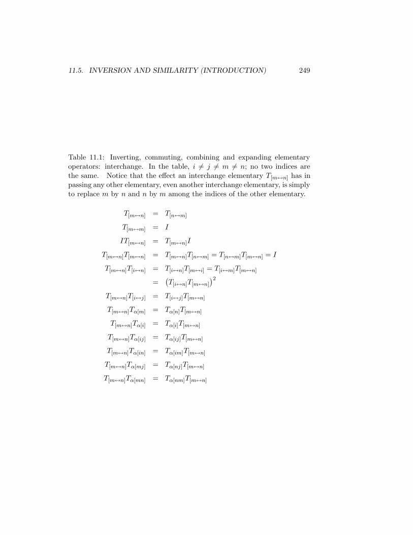
11.5. INVERSION AND SIMILARITY (INTRODUCTION) 249
Table 11.1: Inverting, commuting, combining and expanding elementaryoperators: interchange. In the table, i 6= j 6= m 6= n; no two indices arethe same. Notice that the effect an interchange elementary T[m↔n] has inpassing any other elementary, even another interchange elementary, is simplyto replace m by n and n by m among the indices of the other elementary.
T[m↔n] = T[n↔m]
T[m↔m] = I
IT[m↔n] = T[m↔n]I
T[m↔n]T[m↔n] = T[m↔n]T[n↔m] = T[n↔m]T[m↔n] = I
T[m↔n]T[i↔n] = T[i↔n]T[m↔i] = T[i↔m]T[m↔n]
=(
T[i↔n]T[m↔n]
)2
T[m↔n]T[i↔j] = T[i↔j]T[m↔n]
T[m↔n]Tα[m] = Tα[n]T[m↔n]
T[m↔n]Tα[i] = Tα[i]T[m↔n]
T[m↔n]Tα[ij] = Tα[ij]T[m↔n]
T[m↔n]Tα[in] = Tα[im]T[m↔n]
T[m↔n]Tα[mj] = Tα[nj]T[m↔n]
T[m↔n]Tα[mn] = Tα[nm]T[m↔n]

250 CHAPTER 11. THE MATRIX
Table 11.2: Inverting, commuting, combining and expanding elementaryoperators: scaling. In the table, i 6= j 6= m 6= n; no two indices are thesame.
T1[m] = I
ITβ[m] = Tβ[m]I
T(1/β)[m]Tβ[m] = I
Tβ[m]Tα[m] = Tα[m]Tβ[m] = Tαβ[m]
Tβ[m]Tα[i] = Tα[i]Tβ[m]
Tβ[m]Tα[ij] = Tα[ij]Tβ[m]
Tβ[m]Tαβ[im] = Tα[im]Tβ[m]
Tβ[m]Tα[mj] = Tαβ[mj]Tβ[m]
Table 11.3: Inverting, commuting, combining and expanding elementaryoperators: addition. In the table, i 6= j 6= m 6= n; no two indices are thesame. The last three lines give pairs of addition elementaries that do notcommute.
T0[ij] = I
ITα[ij] = Tα[ij]I
T−α[ij]Tα[ij] = I
Tβ[ij]Tα[ij] = Tα[ij]Tβ[ij] = T(α+β)[ij]
Tβ[mj]Tα[ij] = Tα[ij]Tβ[mj]
Tβ[in]Tα[ij] = Tα[ij]Tβ[in]
Tβ[mn]Tα[ij] = Tα[ij]Tβ[mn]
Tβ[mi]Tα[ij] = Tα[ij]Tαβ[mj]Tβ[mi]
Tβ[jn]Tα[ij] = Tα[ij]T−αβ[in]Tβ[jn]
Tβ[ji]Tα[ij] 6= Tα[ij]Tβ[ji]

11.5. INVERSION AND SIMILARITY (INTRODUCTION) 251
First encountered in § 11.4, the notation T−1 means the inverse of theelementary operator T , such that
T−1T = I = TT−1.
Matrix inversion is not for elementary operators only, though. Many moregeneral matrices C also have inverses such that
C−1C = I = CC−1. (11.45)
(Do all matrices have such inverses? No. For example, the null matrix hasno such inverse.) The broad question of how to invert a general matrix C,we leave for Chs. 12 and 13 to address. For the moment however we shouldlike to observe three simple rules involving matrix inversion.
First, nothing in the logic leading to (11.44) actually requires the ma-trix T there to be an elementary operator. Any matrix C for which C−1 isknown can fill the role. Hence,
CA = [CAC−1]C,
AC = C[C−1AC].(11.46)
The transformation CAC−1 or C−1AC is called a similarity transformation.Section 12.2 speaks further of this.
Second,
(
CT)−1
=(
C−1)T,
(
C∗)−1=(
C−1)∗.
(11.47)
This rule is a consequence of (11.14), since
(
C−1)∗C∗ =
[
CC−1]∗
= [I]∗ = I = [I]∗ =[
C−1C]∗
= C∗ (C−1)∗
and likewise for the transpose.Third,
(
∏
k
Ck
)−1
=∐
k
C−1k . (11.48)
This rule emerges upon repeated application of (11.45), which yields
∐
k
C−1k
∏
k
Ck = I =∏
k
Ck∐
k
C−1k .

252 CHAPTER 11. THE MATRIX
Table 11.4: Matrix inversion properties. (The properties work equally forC−1(r) as for C−1 if A honors an r×r active region. The full notation C−1(r)
for the rank-r inverse is not standard, usually is not needed, and normallyis not used.)
C−1C = I = CC−1
C−1(r)C = Ir = CC−1(r)
CA = [CAC−1]C
AC = C[C−1AC](
CT)−1
=(
C−1)T
(
C∗)−1=
(
C−1)∗
(
∏
k
Ck
)−1
=∐
k
C−1k
A more limited form of the inverse exists than the infinite-dimensionalform of (11.45). This is the rank-r inverse, a matrix C−1(r) such that
C−1(r)C = Ir = CC−1(r). (11.49)
The full notation C−1(r) is not standard and usually is not needed, since thecontext usually implies the rank. When so, one can abbreviate the notationto C−1. In either notation, (11.47) and (11.48) apply equally for the rank-rinverse as for the infinite-dimensional inverse. Because of (11.31), (11.46)too applies for the rank-r inverse if A’s active region is limited to r × r.(Section 13.2 uses the rank-r inverse to solve an exactly determined linearsystem. This is a famous way to use the inverse, with which many or mostreaders will already be familiar; but before using it so in Ch. 13, we shallfirst learn how to compute it reliably in Ch. 12.)
Table 11.4 summarizes.
11.6 Parity
Consider the sequence of integers or other objects 1, 2, 3, . . . , n. By succes-sively interchanging pairs of the objects (any pairs, not just adjacent pairs),

11.6. PARITY 253
one can achieve any desired permutation (§ 4.2.1). For example, beginningwith 1, 2, 3, 4, 5, one can achieve the permutation 3, 5, 1, 4, 2 by interchangingfirst the 1 and 3, then the 2 and 5.
Now contemplate all possible pairs:
(1, 2) (1, 3) (1, 4) · · · (1, n);(2, 3) (2, 4) · · · (2, n);
(3, 4) · · · (3, n);. . .
...(n− 1, n).
In a given permutation (like 3, 5, 1, 4, 2), some pairs will appear in correctorder with respect to one another, while others will appear in incorrect order.(In 3, 5, 1, 4, 2, the pair [1, 2] appears in correct order in that the larger 2stands to the right of the smaller 1; but the pair [1, 3] appears in incorrectorder in that the larger 3 stands to the left of the smaller 1.) If p is thenumber of pairs which appear in incorrect order (in the example, p = 6), andif p is even, then we say that the permutation has even or positive parity; ifodd, then odd or negative parity.23
Now consider: every interchange of adjacent elements must either incre-ment or decrement p by one, reversing parity. Why? Well, think about it.If two elements are adjacent and their order is correct, then interchangingfalsifies the order, but only of that pair (no other element interposes, thusthe interchange affects the ordering of no other pair). Complementarily, ifthe order is incorrect, then interchanging rectifies the order. Either way, anadjacent interchange alters p by exactly ±1, thus reversing parity.
What about nonadjacent elements? Does interchanging a pair of thesereverse parity, too? To answer the question, let u and v represent the two el-ements interchanged, with a1, a2, . . . , am the elements lying between. Beforethe interchange:
. . . , u, a1, a2, . . . , am−1, am, v, . . .
After the interchange:
. . . , v, a1, a2, . . . , am−1, am, u, . . .
The interchange reverses with respect to one another just the pairs
(u, a1) (u, a2) · · · (u, am−1) (u, am)(a1, v) (a2, v) · · · (am−1, v) (am, v)(u, v)
23For readers who learned arithmetic in another language than English, the even integersare . . . ,−4,−2, 0, 2, 4, 6, . . .; the odd integers are . . . ,−3,−1, 1, 3, 5, 7, . . . .

254 CHAPTER 11. THE MATRIX
The number of pairs reversed is odd. Since each reversal alters p by ±1, thenet change in p apparently also is odd, reversing parity. It seems that re-gardless of how distant the pair, interchanging any pair of elements reversesthe permutation’s parity.
The sole exception arises when an element is interchanged with itself.This does not change parity, but it does not change anything else, either, soin parity calculations we ignore it.24 All other interchanges reverse parity.
We discuss parity in this, a chapter on matrices, because parity concernsthe elementary interchange operator of § 11.4. The rows or columns of amatrix can be considered elements in a sequence. If so, then the interchangeoperator T[i↔j], i 6= j, acts precisely in the manner described, interchangingrows or columns and thus reversing parity. It follows that if ik 6= jk and q isodd, then
∏qk=1 T[ik↔jk] 6= I. However, it is possible that
∏qk=1 T[ik↔jk] = I
if q is even. In any event, even q implies even p, which means even (positive)parity; odd q implies odd p, which means odd (negative) parity.
We shall have more to say about parity in §§ 11.7.1 and 13.3.
11.7 The quasielementary operator
Multiplying sequences of the elementary operators of § 11.4, one can formmuch more complicated operators, which per (11.41) are always invertible.Such complicated operators are not trivial to analyze, however, so one findsit convenient to define an intermediate class of operators, called in this bookthe quasielementary operators, more complicated than elementary operatorsbut less so than arbitrary matrices.
A quasielementary operator is composed of elementaries only of a singlekind. There are thus three kinds of quasielementary—interchange, scalingand addition—to match the three kinds of elementary. With respect tointerchange and scaling, any sequences of elementaries of the respective kindsare allowed. With respect to addition, there are some extra rules, explainedin § 11.7.3.
The three subsections which follow respectively introduce the three kindsof quasielementary operator.
24This is why some authors forbid self-interchanges, as explained in footnote 20.

11.7. THE QUASIELEMENTARY OPERATOR 255
11.7.1 The interchange quasielementary or general inter-change operator
Any product P of zero or more interchange elementaries,
P =∏
k
T[ik↔jk], (11.50)
constitutes an interchange quasielementary, permutation matrix or generalinterchange operator.25 An example is
P = T[2↔5]T[1↔3] =
2
6
6
6
6
6
6
6
6
6
6
6
4
. . ....
......
......
· · · 0 0 1 0 0 · · ·· · · 0 0 0 0 1 · · ·· · · 1 0 0 0 0 · · ·· · · 0 0 0 1 0 · · ·· · · 0 1 0 0 0 · · ·
......
......
.... . .
3
7
7
7
7
7
7
7
7
7
7
7
5
.
This operator resembles I in that it has a single one in each row and in eachcolumn, but the ones here do not necessarily run along the main diagonal.The effect of the operator is to shuffle the rows or columns of the matrix itoperates on, without altering any of the rows or columns it shuffles.
By (11.41), (11.39), (11.43) and (11.15), the inverse of the general inter-change operator is
P−1 =
(
∏
k
T[ik↔jk]
)−1
=∐
k
T−1[ik↔jk]
=∐
k
T[ik↔jk]
=∐
k
T ∗[ik↔jk] =
(
∏
k
T[ik↔jk]
)∗
= P ∗ = P T (11.51)
(where P ∗ = P T because P has only real elements). The inverse, transposeand adjoint of the general interchange operator are thus the same:
P TP = P ∗P = I = PP ∗ = PP T
25The letter P here recalls the verb “to permute.”

256 CHAPTER 11. THE MATRIX
A significant attribute of the general interchange operator P is its par-ity: positive or even parity if the number of interchange elementaries T[ik↔jk]
which compose it is even; negative or odd parity if the number is odd. Thisworks precisely as described in § 11.6. For the purpose of parity determina-tion, only interchange elementaries T[ik↔jk] for which ik 6= jk are counted;any T[i↔i] = I noninterchanges are ignored. Thus the example P abovehas even parity (two interchanges), as does I itself (zero interchanges), butT[i↔j] alone (one interchange) has odd parity if i 6= j. As we shall see in§ 13.3, the positive (even) and negative (odd) parities sometimes lend actualpositive and negative senses to the matrices they describe. The parity ofthe general interchange operator P concerns us for this reason.
Parity, incidentally, is a property of the matrix P itself, not just ofthe operation P represents. No interchange quasielementary P has positiveparity as a row operator but negative as a column operator. The reasonis that, regardless of whether one ultimately means to use P as a row orcolumn operator, the matrix is nonetheless composable as a definite sequenceof interchange elementaries. It is the number of interchanges, not the use,which determines P ’s parity.
11.7.2 The scaling quasielementary or general scaling oper-ator
Like the interchange quasielementary, permutation matrix or general inter-change operator P of § 11.7.1, the scaling quasielementary, diagonal matrixor general scaling operator D consists of a product of zero or more elemen-tary operators, in this case elementary scaling operators:26
D =∞∏
i=−∞Tαi[i] =
∞∐
i=−∞Tαi[i] =
2
6
6
6
6
6
6
6
6
6
6
6
4
. . ....
......
......
· · · ∗ 0 0 0 0 · · ·· · · 0 ∗ 0 0 0 · · ·· · · 0 0 ∗ 0 0 · · ·· · · 0 0 0 ∗ 0 · · ·· · · 0 0 0 0 ∗ · · ·
......
......
.... . .
3
7
7
7
7
7
7
7
7
7
7
7
5
(11.52)
(of course it might be that αi = 1, hence that Tαi[i] = I, for some, mostor even all i; however, αi = 0 is forbidden by the definition of the scaling
26The letter D here recalls the adjective “diagonal.”

11.7. THE QUASIELEMENTARY OPERATOR 257
elementary). An example is
D = T−5[4]T4[2]T7[1] =
2
6
6
6
6
6
6
6
6
6
6
6
4
. . ....
......
......
· · · 7 0 0 0 0 · · ·· · · 0 4 0 0 0 · · ·· · · 0 0 1 0 0 · · ·· · · 0 0 0 −5 0 · · ·· · · 0 0 0 0 1 · · ·
......
......
.... . .
3
7
7
7
7
7
7
7
7
7
7
7
5
.
This operator resembles I in that all its entries run down the main diagonal;but these entries, though never zeros, are not necessarily ones, either. Theyare nonzero scaling factors. The effect of the operator is to scale the rowsor columns of the matrix it operates on.
The general scaling operator is a particularly simple matrix. Its inverseis evidently
D−1 =
∞∐
i=−∞T(1/αi)[i] =
∞∏
i=−∞T(1/αi)[i], (11.53)
where each element down the main diagonal is individually inverted.
11.7.3 Addition quasielementaries
Any product of interchange elementaries (§ 11.7.1), any product of scalingelementaries (§ 11.7.2), qualifies as a quasielementary operator. Not so, anyproduct of addition elementaries. To qualify as a quasielementary, a productof elementary addition operators must meet some additional restrictions.
Four types of addition quasielementary are defined:27
27In this subsection the explanations are briefer than in the last two, but the pattern issimilar. The reader can fill in the details.

258 CHAPTER 11. THE MATRIX
• the downward multitarget row addition operator,28
L[j] =
∞∏
i=j+1
Tαij [ij] =
∞∐
i=j+1
Tαij [ij] (11.54)
= I∞ +∞∑
i=j+1
αijEij
=
2
6
6
6
6
6
6
6
6
6
6
6
4
. . ....
......
......
· · · 1 0 0 0 0 · · ·· · · 0 1 0 0 0 · · ·· · · 0 0 1 0 0 · · ·· · · 0 0 ∗ 1 0 · · ·· · · 0 0 ∗ 0 1 · · ·
......
......
.... . .
3
7
7
7
7
7
7
7
7
7
7
7
5
,
whose inverse is
L−1[j] =
∞∐
i=j+1
T−αij [ij] =
∞∏
i=j+1
T−αij [ij] (11.55)
= I∞ −∞∑
i=j+1
αijEij;
• the upward multitarget row addition operator,29
U[j] =
j−1∐
i=−∞Tαij [ij] =
j−1∏
i=−∞Tαij [ij] (11.56)
= I∞ +
j−1∑
i=−∞αijEij
=
2
6
6
6
6
6
6
6
6
6
6
6
4
. . ....
......
......
· · · 1 0 ∗ 0 0 · · ·· · · 0 1 ∗ 0 0 · · ·· · · 0 0 1 0 0 · · ·· · · 0 0 0 1 0 · · ·· · · 0 0 0 0 1 · · ·
......
......
.... . .
3
7
7
7
7
7
7
7
7
7
7
7
5
,
28The letter L here recalls the adjective “lower.”29The letter U here recalls the adjective “upper.”

11.8. THE TRIANGULAR MATRIX 259
whose inverse is
U−1[j] =
j−1∏
i=−∞T−αij [ij] =
j−1∐
i=−∞T−αij [ij] (11.57)
= I∞ −j−1∑
i=−∞αijEij ;
• the rightward multitarget column addition operator, which is the trans-pose LT[j] of the downward operator; and
• the leftward multitarget column addition operator, which is the trans-pose UT
[j] of the upward operator.
11.8 The triangular matrix
Yet more complex than the quasielementary of § 11.7 is the triangular ma-trix, with which we close the chapter:30
L = I +∞∑
i=−∞
i−1∑
j=−∞αijEij = I +
∞∑
j=−∞
∞∑
i=j+1
αijEij (11.58)
=
2
6
6
6
6
6
6
6
6
6
6
6
4
. . ....
......
......
· · · 1 0 0 0 0 · · ·· · · ∗ 1 0 0 0 · · ·· · · ∗ ∗ 1 0 0 · · ·· · · ∗ ∗ ∗ 1 0 · · ·· · · ∗ ∗ ∗ ∗ 1 · · ·
......
......
.... . .
3
7
7
7
7
7
7
7
7
7
7
7
5
;
30Be aware that many or most authors do not require a triangular matrix to have oneson the main diagonal. However, we require it by definition here in this book because itsuits the subsequent development so.
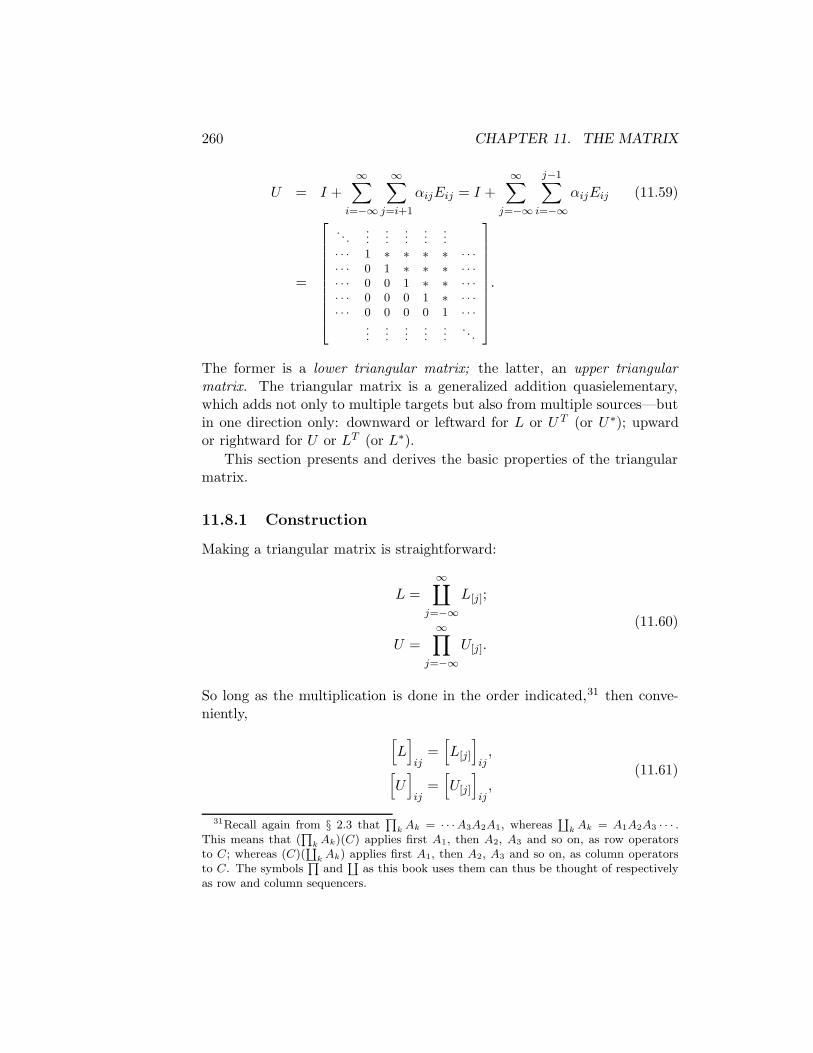
260 CHAPTER 11. THE MATRIX
U = I +∞∑
i=−∞
∞∑
j=i+1
αijEij = I +∞∑
j=−∞
j−1∑
i=−∞αijEij (11.59)
=
2
6
6
6
6
6
6
6
6
6
6
6
4
. . ....
......
......
· · · 1 ∗ ∗ ∗ ∗ · · ·· · · 0 1 ∗ ∗ ∗ · · ·· · · 0 0 1 ∗ ∗ · · ·· · · 0 0 0 1 ∗ · · ·· · · 0 0 0 0 1 · · ·
......
......
.... . .
3
7
7
7
7
7
7
7
7
7
7
7
5
.
The former is a lower triangular matrix; the latter, an upper triangularmatrix. The triangular matrix is a generalized addition quasielementary,which adds not only to multiple targets but also from multiple sources—butin one direction only: downward or leftward for L or U T (or U∗); upwardor rightward for U or LT (or L∗).
This section presents and derives the basic properties of the triangularmatrix.
11.8.1 Construction
Making a triangular matrix is straightforward:
L =∞∐
j=−∞L[j];
U =
∞∏
j=−∞U[j].
(11.60)
So long as the multiplication is done in the order indicated,31 then conve-niently,
[
L]
ij=[
L[j]
]
ij,
[
U]
ij=[
U[j]
]
ij,
(11.61)
31Recall again from § 2.3 thatQ
k Ak = · · ·A3A2A1, whereas‘
k Ak = A1A2A3 · · · .This means that (
Q
k Ak)(C) applies first A1, then A2, A3 and so on, as row operatorsto C; whereas (C)(
‘
k Ak) applies first A1, then A2, A3 and so on, as column operatorsto C. The symbols
Q
and‘
as this book uses them can thus be thought of respectivelyas row and column sequencers.

11.8. THE TRIANGULAR MATRIX 261
which is to say that the entries of L and U are respectively nothing more thanthe relevant entries of the several L[j] and U[j]. Equation (11.61) enables oneto use (11.60) immediately to build any triangular matrix desired.
The correctness of (11.61) is most easily seen if the several L[j] and U[j]
are regarded as column operators acting sequentially on I:
L = (I)
∞∐
j=−∞L[j]
;
U = (I)
∞∏
j=−∞U[j]
.
The reader can construct an inductive proof symbolically on this basis with-out too much difficulty if desired, but just thinking about how L[j] addscolumns leftward and U[j], rightward, then considering the order in whichthe several L[j] and U[j] act, (11.61) follows at once.
11.8.2 The product of like triangular matrices
The product of like triangular matrices,
L1L2 = L,
U1U2 = U,(11.62)
is another triangular matrix of the same type. The proof for lower and uppertriangular matrices is the same. In the lower triangular case, one starts froma form of the definition of a lower triangular matrix:
[L1]ij or [L2]ij =
0 if i < j,
1 if i = j.
Then,
[L1L2]ij =∞∑
m=−∞[L1]im[L2]mj .
But as we have just observed, [L1]im is null when i < m, and [L2]mj is nullwhen m < j. Therefore,
[L1L2]ij =
0 if i < j,∑i
m=j [L1]im[L2]mj if i ≥ j.

262 CHAPTER 11. THE MATRIX
Inasmuch as this is true, nothing prevents us from weakening the statementto read
[L1L2]ij =
0 if i < j,∑i
m=j [L1]im[L2]mj if i = j.
But this is just
[L1L2]ij =
0 if i < j,
[L1]ij [L2]ij = [L1]ii[L2]ii = (1)(1) = 1 if i = j,
which again is the very definition of a lower triangular matrix. Hence (11.62).
11.8.3 Inversion
Inasmuch as any triangular matrix can be constructed from addition quasi-elementaries by (11.60), inasmuch as (11.61) supplies the specific quasiele-mentaries, and inasmuch as (11.55) or (11.57) gives the inverse of each suchquasielementary, one can always invert a triangular matrix easily by
L−1 =
∞∏
j=−∞L−1
[j] ,
U−1 =∞∐
j=−∞U−1
[j] .
(11.63)
In view of (11.62), therefore, the inverse of a lower triangular matrix is an-other lower triangular matrix; and the inverse of an upper triangular matrix,another upper triangular matrix.
It is plain to see but still interesting to note that—unlike the inverse—the adjoint or transpose of a lower triangular matrix is an upper triangularmatrix; and that the adjoint or transpose of an upper triangular matrix isa lower triangular matrix. The adjoint reverses the sense of the triangle.

11.8. THE TRIANGULAR MATRIX 263
11.8.4 The parallel triangular matrix
If a triangular matrix fits the special, restricted form
Lk‖ = I +
k∑
j=−∞
∞∑
i=k+1
αijEij (11.64)
=
2
6
6
6
6
6
6
6
6
6
6
6
4
. . ....
......
......
· · · 1 0 0 0 0 · · ·· · · 0 1 0 0 0 · · ·· · · 0 0 1 0 0 · · ·· · · ∗ ∗ ∗ 1 0 · · ·· · · ∗ ∗ ∗ 0 1 · · ·
......
......
.... . .
3
7
7
7
7
7
7
7
7
7
7
7
5
or
Uk‖ = I +
∞∑
j=k
k−1∑
i=−∞αijEij (11.65)
=
2
6
6
6
6
6
6
6
6
6
6
6
4
. . ....
......
......
· · · 1 0 ∗ ∗ ∗ · · ·· · · 0 1 ∗ ∗ ∗ · · ·· · · 0 0 1 0 0 · · ·· · · 0 0 0 1 0 · · ·· · · 0 0 0 0 1 · · ·
......
......
.... . .
3
7
7
7
7
7
7
7
7
7
7
7
5
,
confining its nonzero elements to a rectangle within the triangle as shown,then it is a parallel triangular matrix and has some special properties thegeneral triangular matrix lacks.
The general lower triangular matrix L acting LA on a matrix A adds the
rows of A downward. The parallel lower triangular matrix Lk‖ acting L
k‖ A
also adds rows downward, but with the useful restriction that it makes norow of A both source and target. The addition is from A’s rows throughthe kth, to A’s (k+1)th row onward. A horizontal frontier separates sourcefrom target, which thus march in A as separate squads.
Similar observations naturally apply with respect to the parallel upper
triangular matrix Uk‖ , which acting U
k‖ A adds rows upward, and also with
respect to LkT‖ and U
kT‖ , which acting AL
kT‖ and AU
kT‖ add columns
respectively rightward and leftward (remembering that LkT‖ is no lower

264 CHAPTER 11. THE MATRIX
but an upper triangular matrix; that UkT‖ is the lower). Each separates
source from target in the matrix A it operates on.
The reason we care about the separation of source from target is that,in matrix arithmetic generally, where source and target are not separatebut remain intermixed, the sequence matters in which rows or columns areadded. That is, in general,
Tα1[i1j1]Tα2[i2j2] 6= I + α1Ei1j1 + α2Ei2j2 6= Tα2[i2j2]Tα1[i1j1].
It makes a difference whether the one addition comes before, during or afterthe other—but only because the target of the one addition might be thesource of the other. The danger is that i1 = j2 or i2 = j1. Remove thisdanger, and the sequence ceases to matter (refer to Table 11.3).
That is exactly what the parallel triangular matrix does: it separatessource from target and thus removes the danger. It is for this reason thatthe parallel triangular matrix brings the useful property that
Lk‖ = I +
k∑
j=−∞
∞∑
i=k+1
αijEij
=
k∐
j=−∞
∞∏
i=k+1
Tαij [ij] =
k∐
j=−∞
∞∐
i=k+1
Tαij [ij]
=
k∏
j=−∞
∞∏
i=k+1
Tαij [ij] =
k∏
j=−∞
∞∐
i=k+1
Tαij [ij]
=∞∏
i=k+1
k∐
j=−∞Tαij [ij] =
∞∐
i=k+1
k∐
j=−∞Tαij [ij]
=
∞∏
i=k+1
k∏
j=−∞Tαij [ij] =
∞∐
i=k+1
k∏
j=−∞Tαij [ij],
Uk‖ = I +
∞∑
j=k
k−1∑
i=−∞αijEij
=∞∏
j=k
k−1∐
i=−∞Tαij [ij] = · · · ,
(11.66)
which says that one can build a parallel triangular matrix equally well in anysequence—in contrast to the case of the general triangular matrix, whose

11.8. THE TRIANGULAR MATRIX 265
construction per (11.60) one must sequence carefully. (Though eqn. 11.66does not show them, even more sequences are possible. You can scramblethe factors’ ordering any random way you like. The multiplication is fullycommutative.) Under such conditions, the inverse of the parallel triangularmatrix is particularly simple:32
Lk−1‖ = I −
k∑
j=−∞
∞∑
i=k+1
αijEij
=k∏
j=−∞
∞∐
i=k+1
T−αij [ij] = · · · ,
Uk−1‖ = I −
∞∑
j=k
k−1∑
i=−∞αijEij
=
∞∐
j=k
k−1∏
i=−∞T−αij [ij] = · · · ,
(11.67)
where again the elementaries can be multiplied in any order. Pictorially,
Lk−1‖ =
2
6
6
6
6
6
6
6
6
6
6
6
4
. . ....
......
......
· · · 1 0 0 0 0 · · ·· · · 0 1 0 0 0 · · ·· · · 0 0 1 0 0 · · ·· · · −∗ −∗ −∗ 1 0 · · ·· · · −∗ −∗ −∗ 0 1 · · ·
......
......
.... . .
3
7
7
7
7
7
7
7
7
7
7
7
5
,
Uk−1‖ =
2
6
6
6
6
6
6
6
6
6
6
6
4
. . ....
......
......
· · · 1 0 −∗ −∗ −∗ · · ·· · · 0 1 −∗ −∗ −∗ · · ·· · · 0 0 1 0 0 · · ·· · · 0 0 0 1 0 · · ·· · · 0 0 0 0 1 · · ·
......
......
.... . .
3
7
7
7
7
7
7
7
7
7
7
7
5
.
The inverse of a parallel triangular matrix is just the matrix itself, only witheach element off the main diagonal negated.
32There is some odd parochiality at play in applied mathematics when one calls suchcollections of symbols as (11.67) “particularly simple.” Nevertheless, in the present contextthe idea (11.67) represents is indeed simple: that one can multiply constituent elementariesin any order and still reach the same parallel triangular matrix; that the elementaries inthis case do not interfere.

266 CHAPTER 11. THE MATRIX
11.8.5 The partial triangular matrix
Besides the notation L and U for the general lower and upper triangular
matrices and the notation Lk‖ and U
k‖ for the parallel lower and upper
triangular matrices, we shall find it useful to introduce the additional nota-tion
L[k] = I +∞∑
j=k
∞∑
i=j+1
αijEij (11.68)
=
2
6
6
6
6
6
6
6
6
6
6
6
4
. . ....
......
......
· · · 1 0 0 0 0 · · ·· · · 0 1 0 0 0 · · ·· · · 0 0 1 0 0 · · ·· · · 0 0 ∗ 1 0 · · ·· · · 0 0 ∗ ∗ 1 · · ·
......
......
.... . .
3
7
7
7
7
7
7
7
7
7
7
7
5
,
U [k] = I +
k∑
j=−∞
j−1∑
i=−∞αijEij (11.69)
=
2
6
6
6
6
6
6
6
6
6
6
6
4
. . ....
......
......
· · · 1 ∗ ∗ 0 0 · · ·· · · 0 1 ∗ 0 0 · · ·· · · 0 0 1 0 0 · · ·· · · 0 0 0 1 0 · · ·· · · 0 0 0 0 1 · · ·
......
......
.... . .
3
7
7
7
7
7
7
7
7
7
7
7
5
,
Lk = I +
k∑
j=−∞
∞∑
i=j+1
αijEij (11.70)
=
2
6
6
6
6
6
6
6
6
6
6
6
4
. . ....
......
......
· · · 1 0 0 0 0 · · ·· · · ∗ 1 0 0 0 · · ·· · · ∗ ∗ 1 0 0 · · ·· · · ∗ ∗ ∗ 1 0 · · ·· · · ∗ ∗ ∗ 0 1 · · ·
......
......
.... . .
3
7
7
7
7
7
7
7
7
7
7
7
5
,

11.9. THE SHIFT OPERATOR 267
Uk = I +∞∑
j=k
j−1∑
i=−∞αijEij (11.71)
=
2
6
6
6
6
6
6
6
6
6
6
6
4
. . ....
......
......
· · · 1 0 ∗ ∗ ∗ · · ·· · · 0 1 ∗ ∗ ∗ · · ·· · · 0 0 1 ∗ ∗ · · ·· · · 0 0 0 1 ∗ · · ·· · · 0 0 0 0 1 · · ·
......
......
.... . .
3
7
7
7
7
7
7
7
7
7
7
7
5
.
Such notation is not standard in the literature, but it serves a purpose inthis book and is introduced here for this reason. If names are needed for L[k],U [k], Lk and Uk, the former pair can be called minor partial triangularmatrices, and the latter pair, major partial triangular matrices. Whetherminor or major, the partial triangular matrix is a matrix which leftwardor rightward of the kth column resembles I. Of course partial triangularmatrices which resemble I above or below the kth row are equally possible,and can be denoted L[k]T , U [k]T , LkT and UkT .
Observe that the parallel triangular matrices Lk‖ and U
k‖ of § 11.8.4
are in fact also major partial triangular matrices, as the notation suggests.
11.9 The shift operator
Not all useful matrices fit the dimension-limited and extended-operationalforms of § 11.3. An exception is the shift operator Hk, defined that
[Hk]ij = δi(j+k). (11.72)
For example,
H2 =
2
6
6
6
6
6
6
6
6
6
6
6
6
6
6
6
4
......
......
......
...· · · 0 0 0 0 0 0 0 · · ·· · · 0 0 0 0 0 0 0 · · ·· · · 1 0 0 0 0 0 0 · · ·· · · 0 1 0 0 0 0 0 · · ·· · · 0 0 1 0 0 0 0 · · ·· · · 0 0 0 1 0 0 0 · · ·· · · 0 0 0 0 1 0 0 · · ·
......
......
......
...
3
7
7
7
7
7
7
7
7
7
7
7
7
7
7
7
5
.

268 CHAPTER 11. THE MATRIX
Operating HkA, Hk shifts A’s rows downward k steps. Operating AHk, Hk
shifts A’s columns leftward k steps. Inasmuch as the shift operator shiftsall rows or columns of the matrix it operates on, its active region is ∞×∞in extent. Obviously, the shift operator’s inverse, transpose and adjoint arethe same:
HTk Hk = H∗
kHk = I = HkH∗k = HkH
Tk ,
H−1k = H−k.
(11.73)
The shift operator completes the family of matrix rudiments we shallneed to begin to do increasingly interesting things with matrices in Chs. 13and 14. Before doing interesting things, however, we must treat two morefoundational matrix matters. The two are the Gauss-Jordan factorizationand the matter of matrix rank, which will be the subjects of Ch. 12, next.
Chapter 12
Matrix rank and theGauss-Jordan factorization
Chapter 11 has brought the matrix and its rudiments, the latter including
• lone-element matrix E (§ 11.3.7),
• the null matrix 0 (§ 11.3.1),
• the rank-r identity matrix Ir (§ 11.3.5),
• the general identity matrix I and the scalar matrix λI (§ 11.3.2),
• the elementary operator T (§ 11.4),
• the quasielementary operator P , D, L[k] or U[k] (§ 11.7), and
• the triangular matrix L or U (§ 11.8).
Such rudimentary forms have useful properties, as we have seen. The generalmatrix A does not necessarily have any of these properties, but it turns outthat one can factor any matrix whatsoever into a product of rudiments whichdo have the properties, and that several orderly procedures are known todo so. The simplest of these, and indeed one of the more useful, is theGauss-Jordan factorization. This chapter introduces it.
Section 11.3 has deemphasized the concept of matrix dimensionality m×n, supplying in its place the new concept of matrix rank. However, thatsection has actually defined rank only for the rank-r identity matrix Ir. Infact all matrices have rank. This chapter explains.
Before treating the Gauss-Jordan factorization and the matter of matrixrank as such, however, we shall find it helpful to prepare two preliminaries
269

270 CHAPTER 12. RANK AND THE GAUSS-JORDAN
thereto: (i) the matter of the linear independence of vectors; and (ii) theelementary similarity transformation. The chapter begins with these.
Except in § 12.2, the chapter demands more rigor than one likes in sucha book as this. However, it is hard to see how to avoid the rigor here, andlogically the chapter cannot be omitted. We shall drive through the chapterin as few pages as can be managed, and then onward to the more interestingmatrix topics of Chs. 13 and 14.
12.1 Linear independence
Linear independence is a significant possible property of a set of vectors—whether the set be the several columns of a matrix, the several rows, orsome other vectors—the property being defined as follows. A vector is lin-early independent if its role cannot be served by the other vectors in theset. More formally, the n vectors of the set a1,a2,a3,a4,a5, . . . ,an arelinearly independent if and only if none of them can be expressed as a linearcombination—a weighted sum—of the others. That is, the several ak arelinearly independent iff
α1a1 + α2a2 + α3a3 + · · ·+ αnan 6= 0 (12.1)
for all nontrivial αk, where “nontrivial αk” means the several αk, at leastone of which is nonzero (trivial αk, by contrast, would be α1 = α2 = α3 =· · · = αn = 0). Vectors which can combine nontrivially to reach the nullvector are by definition linearly dependent.
Linear independence is a property of vectors. Technically the propertyapplies to scalars, too, inasmuch as a scalar resembles a one-element vector—so, any nonzero scalar alone is linearly independent—but there is no suchthing as a linearly independent pair of scalars, because one of the pair canalways be expressed as a complex multiple of the other. Significantly butless obviously, there is also no such thing as a linearly independent set whichincludes the null vector; (12.1) forbids it. Paradoxically, even the single-member, n = 1 set consisting only of a1 = 0 is, strictly speaking, notlinearly independent.
For consistency of definition, we regard the empty, n = 0 set as linearlyindependent, on the technical ground that the only possible linear combina-tion of the empty set is trivial.1
1This is the kind of thinking which typically governs mathematical edge cases. Onecould define the empty set to be linearly dependent if one really wanted to, but what

12.1. LINEAR INDEPENDENCE 271
If a linear combination of several independent vectors ak forms a vec-tor b, then one might ask: can there exist a different linear combination ofthe same vectors ak which also forms b? That is, if
β1a1 + β2a2 + β3a3 + · · ·+ βnan = b,
where the several ak satisfy (12.1), then is
β′1a1 + β′2a2 + β′3a3 + · · ·+ β′nan = b
possible? To answer the question, suppose that it were possible. The differ-ence of the two equations then would be
(β′1 − β1)a1 + (β′2 − β2)a2 + (β′3 − β3)a3 + · · ·+ (β′n − βn)an = 0.
According to (12.1), this could only be so if the coefficients in the lastequation where trivial—that is, only if β ′
1 − β1 = 0, β′2 − β2 = 0, β′
3 −β3 = 0, . . . , β ′
n − βn = 0. But this says no less than that the two linearcombinations, which we had supposed to differ, were in fact one and thesame. One concludes therefore that, if a vector b can be expressed as alinear combination of several linearly independent vectors ak, then it cannotbe expressed as any other combination of the same vectors. The combinationis unique.
Linear independence can apply in any dimensionality, but it helps tovisualize the concept geometrically in three dimensions, using the three-dimensional geometrical vectors of § 3.3. Two such vectors are independentso long as they do not lie along the same line. A third such vector isindependent of the first two so long as it does not lie in their common plane.A fourth such vector (unless it points off into some unvisualizable fourthdimension) cannot possibly then be independent of the three.
We discuss the linear independence of vectors in this, a chapter on ma-trices, because (§ 11.1) a matrix is essentially a sequence of vectors—eitherof column vectors or of row vectors, depending on one’s point of view. Aswe shall see in § 12.5, the important property of matrix rank depends onthe number of linearly independent columns or rows a matrix has.
then of the observation that adding a vector to a linearly dependent set never rendersthe set independent? Surely in this light it is preferable just to define the empty set asindependent in the first place. Similar thinking makes 0! = 1,
P−1k=0 akz
k = 0, and 2 not 1the least prime, among other examples.

272 CHAPTER 12. RANK AND THE GAUSS-JORDAN
12.2 The elementary similarity transformation
Section 11.5 and its (11.46) have introduced the similarity transformationCAC−1 or C−1AC, which arises when an operator C commutes respectivelyrightward or leftward past a matrix A. The similarity transformation hasseveral interesting properties, some of which we are now prepared to discuss,particularly in the case in which the operator happens to be an elementary,C = T . In this case, the several rules of Table 12.1 obtain.
Most of the table’s rules are fairly obvious if the meaning of the symbolsis understood, though to grasp some of the rules it helps to sketch therelevant matrices on a sheet of paper. Of course rigorous symbolic proofscan be constructed after the pattern of § 11.8.2, but they reveal little ornothing sketching the matrices does not. The symbols P , D, L and U ofcourse represent the quasielementaries and triangular matrices of §§ 11.7and 11.8. The symbols P ′, D′, L′ and U ′ also represent quasielementariesand triangular matrices, only not necessarily the same ones P , D, L and Udo.
The rules permit one to commute some but not all elementaries past aquasielementary or triangular matrix, without fundamentally altering thecharacter of the quasielementary or triangular matrix, and sometimes with-out altering the matrix at all. The rules find use among other places in theGauss-Jordan factorization of § 12.3.
12.3 The Gauss-Jordan factorization
The Gauss-Jordan factorization of an arbitrary, dimension-limited, m × nmatrix A is2
A = C>IrC<
= PDLUIrKS,
C< ≡ KS,C> ≡ PDLU,
(12.2)
where
• P and S are general interchange operators (§ 11.7.1);
2Most introductory linear algebra texts this writer has met call the Gauss-Jordan fac-torization instead the “LU factorization” and include fewer factors in it, typically merg-ing D into L and omitting K and S. They also omit Ir, since their matrices have pre-defined dimensionality. Perhaps the reader will agree that the factorization is cleaner aspresented here.

12.3. THE GAUSS-JORDAN FACTORIZATION 273
Table 12.1: Some elementary similarity transformations.
T[i↔j]IT[i↔j] = I
T[i↔j]PT[i↔j] = P ′
T[i↔j]DT[i↔j] = D′ = D + ([D]jj − [D]ii)Eii + ([D]ii − [D]jj)Ejj
T[i↔j]DT[i↔j] = D if [D]ii = [D]jj
T[i↔j]L[k]T[i↔j] = L[k] if i < k and j < k
T[i↔j]U[k]T[i↔j] = U [k] if i > k and j > k
T[i↔j]LkT[i↔j] = Lk′ if i > k and j > k
T[i↔j]UkT[i↔j] = Uk′ if i < k and j < k
T[i↔j]Lk‖ T[i↔j] = L
k‖
′if i > k and j > k
T[i↔j]Uk‖ T[i↔j] = U
k‖
′if i < k and j < k
Tα[i]IT(1/α)[i] = I
Tα[i]DT(1/α)[i] = D
Tα[i]AT(1/α)[i] = A′ where A is any of
L,U,L[k], U [k], Lk, Uk, Lk‖ , U
k‖
Tα[ij]IT−α[ij] = I
Tα[ij]DT−α[ij] = D + ([D]jj − [D]ii)αEij 6= D′
Tα[ij]DT−α[ij] = D if [D]ii = [D]jj
Tα[ij]LT−α[ij] = L′ if i > j
Tα[ij]UT−α[ij] = U ′ if i < j

274 CHAPTER 12. RANK AND THE GAUSS-JORDAN
• D is a general scaling operator (§ 11.7.2);
• L and U are respectively lower and upper triangular matrices (§ 11.8);
• K = LrT‖ is the transpose of a parallel lower triangular matrix, being
thus a parallel upper triangular matrix (§ 11.8.4);
• C> and C< are composites as defined by (12.2); and
• r is an unspecified rank.
Whether all possible matrices A have a Gauss-Jordan factorization (they do,in fact) is a matter this section addresses. However—at least for matriceswhich do have one—because C> and C< are composed of invertible factors,one can left-multiply the equation A = C>IrC< by C−1
> and right-multiplyit by C−1
< to obtain
U−1L−1D−1P−1AS−1K−1 =
C−1> AC−1
< = Ir,
S−1K−1 = C−1< ,
U−1L−1D−1P−1 = C−1> ,
(12.3)
the Gauss-Jordan’s complementary form.
12.3.1 Motive
Equation (12.2) seems inscrutable. The equation itself is easy enough toread, but just as there are many ways to factor a scalar (0xC = [4][3] =[2]2[3] = [2][6], for example), there are likewise many ways to factor a matrix.Why choose this particular way?
There are indeed many ways. We shall meet some of the others in Ch. 14.The Gauss-Jordan factorization we meet here however has both significanttheoretical properties and useful practical applications, and in any case needsless advanced preparation to appreciate than the others, and (at least asdeveloped in this book) precedes the others logically. It emerges naturallywhen one posits a pair of square, n × n matrices, A and A−1, for whichA−1A = In, where A is known and A−1 is to be determined. (The A−1
here is the A−1(n) of eqn. 11.49. However, it is only supposed here thatA−1A = In; it is not yet claimed that AA−1 = In.)
To determine A−1 is not an entirely trivial problem. The matrix A−1
such that A−1A = In may or may not exist (usually it does exist if A is

12.3. THE GAUSS-JORDAN FACTORIZATION 275
square, but even then it may not, as we shall soon see), and even if it doesexist, how to determine it is not immediately obvious. And still, if onecan determine A−1, that is only for square A; what if A is not square? Inthe present subsection however we are not trying to prove anything, onlyto motivate, so for the moment let us suppose a square A for which A−1
does exist, and let us seek A−1 by left-multiplying A by a sequence∏
Tof elementary row operators, each of which makes the matrix more nearlyresemble In. When In is finally achieved, then we shall have that
(
∏
T)
(A) = In,
or, left-multiplying by In and observing that I2n = In,
(In)(
∏
T)
(A) = In,
which implies that
A−1 = (In)(
∏
T)
.
The product of elementaries which transforms A to In, truncated (§ 11.3.6)to n × n dimensionality, itself constitutes A−1. This observation is whatmotivates the Gauss-Jordan factorization.
By successive steps,3 a concrete example:
A =»
2 −43 −1
–
,»
12
00 1
–
A =»
1 −23 −1
–
,»
1 0−3 1
– »
12
00 1
–
A =»
1 −20 5
–
,»
1 00 1
5
– »
1 0−3 1
– »
12
00 1
–
A =»
1 −20 1
–
,»
1 20 1
– »
1 00 1
5
– »
1 0−3 1
– »
12
00 1
–
A =»
1 00 1
–
,»
1 00 1
– »
1 20 1
– »
1 00 1
5
– »
1 0−3 1
– »
12
00 1
–
A =»
1 00 1
–
.
Hence,
A−1 =
"
1 0
0 1
# "
1 2
0 1
# "
1 0
0 15
# "
1 0
−3 1
# "
12
0
0 1
#
=
"
− 1A
25
− 3A
15
#
.
3Theoretically, all elementary operators including the ones here have extended-operational form (§ 11.3.2), but all those · · · ellipses clutter the page too much. Onlythe 2 × 2 active regions are shown here.

276 CHAPTER 12. RANK AND THE GAUSS-JORDAN
Using the elementary commutation identity that Tβ[m]Tα[mj] = Tαβ[mj]Tβ[m],from Table 11.2, to group like operators, we have that
A−1 =
"
1 0
0 1
# "
1 2
0 1
# "
1 0
− 35
1
# "
1 0
0 15
# "
12
0
0 1
#
=
"
− 1A
25
− 3A
15
#
;
or, multiplying the two scaling elementaries to merge them into a singlegeneral scaling operator (§ 11.7.2),
A−1 =
"
1 0
0 1
# "
1 2
0 1
# "
1 0
− 35
1
# "
12
0
0 15
#
=
"
− 1A
25
− 3A
15
#
.
The last equation is written symbolically as
A−1 = I2U−1L−1D−1,
from which
A = DLUI2 =»
2 00 5
– »
1 035
1
– »
1 −20 1
– »
1 00 1
–
=»
2 −43 −1
–
.
Now, admittedly, the equation A = DLUI2 is not (12.2)—or rather, itis (12.2), but only in the special case that r = 2 and P = S = K = I—whichbegs the question: why do we need the factors P , S and K in the first place?The answer regarding P and S is that these factors respectively gather rowand column interchange elementaries, of which the example given has usednone but which other examples sometimes need or want, particularly toavoid dividing by zero when they encounter a zero in an inconvenient cell ofthe matrix (the reader might try reducing A = [0 1; 1 0] to I2, for instance; arow or column interchange is needed here). Regarding K, this factor comesinto play when A has broad rectangular rather than square shape, and alsosometimes when one of the rows of A happens to be a linear combinationof the others. The last point, we are not quite ready to detail yet, butat present we are only motivating not proving, so if the reader will acceptthe other factors and suspend judgment on K until the actual need for itemerges in § 12.3.3, step 12, then we shall proceed on this basis.
12.3.2 Method
The Gauss-Jordan factorization of a matrix A is not discovered at one strokebut rather is gradually built up, elementary by elementary. It begins withthe equation
A = IIIIAII,

12.3. THE GAUSS-JORDAN FACTORIZATION 277
where the six I hold the places of the six Gauss-Jordan factors P , D, L, U ,K and S of (12.2). By successive elementary operations, the A is graduallytransformed into Ir, while the six I are gradually transformed into the sixGauss-Jordan factors. The factorization thus ends with the equation
A = PDLUIrKS,
which is (12.2). In between, while the several matrices are gradually beingtransformed, the equation is represented as
A = P DLU IKS, (12.4)
where the initial value of I is A and the initial values of P , D, etc., are all I.
Each step of the transformation goes as follows. The matrix I is left- orright-multiplied by an elementary operator T . To compensate, one of thesix factors is right- or left-multiplied by T−1. Intervening factors are mul-tiplied by both T and T−1, which multiplication constitutes an elementarysimilarity transformation as described in § 12.2. For example,
A = P(
DT(1/α)[i]
)(
Tα[i]LT(1/α)[i]
)(
Tα[i]UT(1/α)[i]
)(
Tα[i]I)
KS,
which is just (12.4), inasmuch as the adjacent elementaries cancel one an-other; then,
I ← Tα[i]I ,
U ← Tα[i]UT(1/α)[i],
L ← Tα[i]LT(1/α)[i],
D ← DT(1/α)[i],
thus associating the operation with the appropriate factor—in this case, D.Such elementary row and column operations are repeated until I = Ir, atwhich point (12.4) has become the Gauss-Jordan factorization (12.2).
12.3.3 The algorithm
Having motivated the Gauss-Jordan factorization in § 12.3.1 and havingproposed a basic method to pursue it in § 12.3.2, we shall now establish adefinite, orderly, failproof algorithm to achieve it. Broadly, the algorithm
• copies A into the variable working matrix I (step 1 below),

278 CHAPTER 12. RANK AND THE GAUSS-JORDAN
• reduces I by suitable row (and maybe column) operations to uppertriangular form (steps 2 through 7),
• establishes a rank r (step 8), and
• reduces the now triangular I further to the rank-r identity matrix Ir(steps 9 through 13).
Specifically, the algorithm decrees the following steps. (The steps as writteninclude many parenthetical remarks—so many that some steps seem to con-sist more of parenthetical remarks than of actual algorithm. The remarksare unnecessary to execute the algorithm’s steps as such. They are howevernecessary to explain and to justify the algorithm’s steps to the reader.)
1. Begin by initializing
P ← I,
D ← I,
L ← I,
U ← I,
I ← A,
K ← I,
S ← I,
i ← 1,
where I holds the part of A remaining to be factored, where i is a rowindex, and where the others are the variable working matrices of (12.4).(The eventual goal will be to factor all of I away, leaving I = Ir,though the precise value of r will not be known until step 8. Since Aby definition is a dimension-limited m× n matrix, one naturally neednot store A beyond the m × n active region. What is less clear untilone has read the whole algorithm, but nevertheless true, is that onealso need not store the dimension-limited I beyond the m× n activeregion. The other six variable working matrices each have extended-operational form, but they also confine their activity to well definedregions: m×m for P , D, L and U ; n×n for K and S. One need storenone of the matrices beyond these bounds.)
2. (Besides arriving at this point from step 1 above, the algorithm alsoreenters here from step 7 below. From step 1, I = A and L = I, sothis step 2 though logical seems unneeded. The need grows clear once

12.3. THE GAUSS-JORDAN FACTORIZATION 279
one has read through step 7.) Observe that neither the ith row of Inor any row below it has an entry left of the ith column, that I isall-zero below-leftward of and directly leftward of (though not directlybelow) the pivot element ı ii.
4 Observe also that above the ith row,the matrix has proper upper triangular form (§ 11.8). Regarding theother factors, notice that L enjoys the major partial triangular formLi−1 (§ 11.8.5) and that dkk = 1 for all k ≥ i. Pictorially,
D =
2
6
6
6
6
6
6
6
6
6
6
6
6
6
6
6
4
. . ....
......
......
......
· · · ∗ 0 0 0 0 0 0 · · ·· · · 0 ∗ 0 0 0 0 0 · · ·· · · 0 0 ∗ 0 0 0 0 · · ·· · · 0 0 0 1 0 0 0 · · ·· · · 0 0 0 0 1 0 0 · · ·· · · 0 0 0 0 0 1 0 · · ·· · · 0 0 0 0 0 0 1 · · ·
......
......
......
.... . .
3
7
7
7
7
7
7
7
7
7
7
7
7
7
7
7
5
,
L = Li−1 =
2
6
6
6
6
6
6
6
6
6
6
6
6
6
6
6
4
. . ....
......
......
......
· · · 1 0 0 0 0 0 0 · · ·· · · ∗ 1 0 0 0 0 0 · · ·· · · ∗ ∗ 1 0 0 0 0 · · ·· · · ∗ ∗ ∗ 1 0 0 0 · · ·· · · ∗ ∗ ∗ 0 1 0 0 · · ·· · · ∗ ∗ ∗ 0 0 1 0 · · ·· · · ∗ ∗ ∗ 0 0 0 1 · · ·
......
......
......
.... . .
3
7
7
7
7
7
7
7
7
7
7
7
7
7
7
7
5
,
I =
2
6
6
6
6
6
6
6
6
6
6
6
6
6
6
6
4
. . ....
......
......
......
· · · 1 ∗ ∗ ∗ ∗ ∗ ∗ · · ·· · · 0 1 ∗ ∗ ∗ ∗ ∗ · · ·· · · 0 0 1 ∗ ∗ ∗ ∗ · · ·· · · 0 0 0 ∗ ∗ ∗ ∗ · · ·· · · 0 0 0 ∗ ∗ ∗ ∗ · · ·· · · 0 0 0 ∗ ∗ ∗ ∗ · · ·· · · 0 0 0 ∗ ∗ ∗ ∗ · · ·
......
......
......
.... . .
3
7
7
7
7
7
7
7
7
7
7
7
7
7
7
7
5
,
where the ith row and ith column are depicted at center.
4The notation ıii looks interesting, but this is accidental. The ı relates not to thedoubled, subscribed index ii but to I. The notation ıii thus means [I]ii—in other words,it means the current iith element of the variable working matrix I.

280 CHAPTER 12. RANK AND THE GAUSS-JORDAN
3. Choose a nonzero element ıpq 6= 0 on or below the pivot row, wherep ≥ i and q ≥ i. (The easiest choice may simply be ı ii, where p =q = i, if ıii 6= 0; but any nonzero element from the ith row downwardcan in general be chosen. Beginning students of the Gauss-Jordanor LU factorization are conventionally taught to choose first the leastpossible q then the least possible p. When one has no reason to chooseotherwise, that is as good a choice as any. There is however no actualneed to choose so. In fact alternate choices can sometimes improvepractical numerical accuracy.5 Theoretically nonetheless, when doingexact arithmetic, the choice is quite arbitrary, so long as ıpq 6= 0.) Ifno nonzero element is available—if all remaining rows p ≥ i are nownull—then skip directly to step 8.
4. Observing that (12.4) can be expanded to read
A =(
P T[p↔i]
)(
T[p↔i]DT[p↔i]
)(
T[p↔i]LT[p↔i]
)(
T[p↔i]UT[p↔i]
)
×(
T[p↔i]ITT[i↔q]
)(
T T[i↔q]KTT[i↔q]
)(
T T[i↔q]S)
=(
P T[p↔i]
)
D(
T[p↔i]LT[p↔i]
)
U
×(
T[p↔i]ITT[i↔q]
)
K(
T T[i↔q]S)
,
let6
P ← P T[p↔i],
L ← T[p↔i]LT[p↔i],
I ← T[p↔i]ITT[i↔q],
S ← T T[i↔q]S,
5A typical Intel or AMD x86-class computer processor represents a C/C++ double-type floating-point number, x = 2pb, in 0x40 bits of computer memory. Of the 0x40bits, 0x34 are for the number’s mantissa 2.0 ≤ b < 4.0 (not 1.0 ≤ b < 2.0 as one mightexpect), 0xB are for the number’s exponent −0x3FF ≤ p ≤ 0x3FE, and one is for thenumber’s ± sign. (The mantissa’s high-order bit, which is always 1, is implied not stored,thus is one neither of the 0x34 nor of the 0x40 bits.) The out-of-bounds exponents p =−0x400 and p = 0x3FF serve specially respectively to encode 0 and∞. All this is standardcomputing practice. Such a floating-point representation is easily accurate enough for mostpractical purposes, but of course it is not generally exact. [22, § 1-4.2.2]
6The transposition [·]T here doesn’t really do anything, inasmuch as an interchangeelementary per (11.43) is already its own transpose; but at least it reminds us that T T
[i↔q]
is being used to interchange columns not rows. You can write it just as T[i↔q] if you want.Note that in addition to being its own transpose, the interchange elementary is also itsown inverse.

12.3. THE GAUSS-JORDAN FACTORIZATION 281
thus interchanging the pth with the ith row and the qth with theith column, to bring the chosen element to the pivot position. (Re-fer to Table 12.1 for the similarity transformations. The U and Ktransformations disappear because at this stage of the algorithm, stillU = K = I. The D transformation disappears because p ≥ i andbecause dkk = 1 for all k ≥ i. Regarding the L transformation, it doesnot disappear, but L has major partial triangular form Li−1, whichform according to Table 12.1 it retains since i− 1 < i ≤ p.)
5. Observing that (12.4) can be expanded to read
A = P(
DTıii[i]
)(
T(1/ı ii)[i]LTıii[i]
)(
T(1/ı ii)[i]U Tıii[i]
)
×(
T(1/ı ii)[i]I)
KS
= P(
DTıii[i]
)(
T(1/ı ii)[i]LTıii[i]
)
U(
T(1/ı ii)[i]I)
KS,
normalize the new ı ii pivot by letting
D ← DTıii[i],
L ← T(1/ı ii)[i]LTıii[i],
I ← T(1/ı ii)[i]I .
This forces ıii = 1. It also changes the value of dii. Pictorially afterthis step,
D =
2
6
6
6
6
6
6
6
6
6
6
6
6
6
6
6
4
. . ....
......
......
......
· · · ∗ 0 0 0 0 0 0 · · ·· · · 0 ∗ 0 0 0 0 0 · · ·· · · 0 0 ∗ 0 0 0 0 · · ·· · · 0 0 0 ∗ 0 0 0 · · ·· · · 0 0 0 0 1 0 0 · · ·· · · 0 0 0 0 0 1 0 · · ·· · · 0 0 0 0 0 0 1 · · ·
......
......
......
.... . .
3
7
7
7
7
7
7
7
7
7
7
7
7
7
7
7
5
,
I =
2
6
6
6
6
6
6
6
6
6
6
6
6
6
6
6
4
. . ....
......
......
......
· · · 1 ∗ ∗ ∗ ∗ ∗ ∗ · · ·· · · 0 1 ∗ ∗ ∗ ∗ ∗ · · ·· · · 0 0 1 ∗ ∗ ∗ ∗ · · ·· · · 0 0 0 1 ∗ ∗ ∗ · · ·· · · 0 0 0 ∗ ∗ ∗ ∗ · · ·· · · 0 0 0 ∗ ∗ ∗ ∗ · · ·· · · 0 0 0 ∗ ∗ ∗ ∗ · · ·
......
......
......
.... . .
3
7
7
7
7
7
7
7
7
7
7
7
7
7
7
7
5
.

282 CHAPTER 12. RANK AND THE GAUSS-JORDAN
(Though the step changes L, too, again it leaves L in the major partialtriangular form Li−1, because i− 1 < i. Refer to Table 12.1.)
6. Observing that (12.4) can be expanded to read
A = P D(
LTıpi[pi]
)(
T−ıpi[pi]U Tıpi[pi]
)(
T−ıpi[pi]I)
KS
= P D(
LTıpi[pi]
)
U(
T−ıpi[pi]I)
KS,
clear I’s ith column below the pivot by letting
L ←(
L)
m∐
p=i+1
Tıpi[pi]
,
I ←
m∏
p=i+1
T−ıpi[pi]
(
I)
.
This forces ı ip = 0 for all p > i. It also fills in L’s ith column below thepivot, advancing that matrix from the Li−1 form to the Li form.Pictorially,
L = Li =
2
6
6
6
6
6
6
6
6
6
6
6
6
6
6
6
4
. . ....
......
......
......
· · · 1 0 0 0 0 0 0 · · ·· · · ∗ 1 0 0 0 0 0 · · ·· · · ∗ ∗ 1 0 0 0 0 · · ·· · · ∗ ∗ ∗ 1 0 0 0 · · ·· · · ∗ ∗ ∗ ∗ 1 0 0 · · ·· · · ∗ ∗ ∗ ∗ 0 1 0 · · ·· · · ∗ ∗ ∗ ∗ 0 0 1 · · ·
......
......
......
.... . .
3
7
7
7
7
7
7
7
7
7
7
7
7
7
7
7
5
,
I =
2
6
6
6
6
6
6
6
6
6
6
6
6
6
6
6
4
. . ....
......
......
......
· · · 1 ∗ ∗ ∗ ∗ ∗ ∗ · · ·· · · 0 1 ∗ ∗ ∗ ∗ ∗ · · ·· · · 0 0 1 ∗ ∗ ∗ ∗ · · ·· · · 0 0 0 1 ∗ ∗ ∗ · · ·· · · 0 0 0 0 ∗ ∗ ∗ · · ·· · · 0 0 0 0 ∗ ∗ ∗ · · ·· · · 0 0 0 0 ∗ ∗ ∗ · · ·
......
......
......
.... . .
3
7
7
7
7
7
7
7
7
7
7
7
7
7
7
7
5
.
(Note that it is not necessary actually to apply the addition elemen-taries here one by one. Together they easily form an addition quasiel-ementary L[i], thus can be applied all at once. See § 11.7.3.)

12.3. THE GAUSS-JORDAN FACTORIZATION 283
7. Incrementi← i+ 1.
Go back to step 2.
8. Decrementi← i− 1
to undo the last instance of step 7 (even if there never was an instanceof step 7), thus letting i point to the matrix’s last nonzero row. Afterdecrementing, let the rank
r ≡ i.Notice that, certainly, r ≤ m and r ≤ n.
9. (Besides arriving at this point from step 8 above, the algorithm alsoreenters here from step 11 below.) If i = 0, then skip directly tostep 12.
10. Observing that (12.4) can be expanded to read
A = P DL(
U Tıpi[pi]
)(
T−ıpi[pi]I)
KS,
clear I ’s ith column above the pivot by letting
U ←(
U)
i−1∏
p=1
Tıpi[pi]
,
I ←
i−1∐
p=1
T−ıpi[pi]
(
I)
.
This forces ıip = 0 for all p 6= i. It also fills in U ’s ith column above thepivot, advancing that matrix from the U i+1 form to the U i form.Pictorially,
U = Ui =
2
6
6
6
6
6
6
6
6
6
6
6
6
6
6
6
4
. . ....
......
......
......
· · · 1 0 0 ∗ ∗ ∗ ∗ · · ·· · · 0 1 0 ∗ ∗ ∗ ∗ · · ·· · · 0 0 1 ∗ ∗ ∗ ∗ · · ·· · · 0 0 0 1 ∗ ∗ ∗ · · ·· · · 0 0 0 0 1 ∗ ∗ · · ·· · · 0 0 0 0 0 1 ∗ · · ·· · · 0 0 0 0 0 0 1 · · ·
......
......
......
.... . .
3
7
7
7
7
7
7
7
7
7
7
7
7
7
7
7
5
,

284 CHAPTER 12. RANK AND THE GAUSS-JORDAN
I =
2
6
6
6
6
6
6
6
6
6
6
6
6
6
6
6
4
. . ....
......
......
......
· · · 1 ∗ ∗ 0 0 0 0 · · ·· · · 0 1 ∗ 0 0 0 0 · · ·· · · 0 0 1 0 0 0 0 · · ·· · · 0 0 0 1 0 0 0 · · ·· · · 0 0 0 0 1 0 0 · · ·· · · 0 0 0 0 0 1 0 · · ·· · · 0 0 0 0 0 0 1 · · ·
......
......
......
.... . .
3
7
7
7
7
7
7
7
7
7
7
7
7
7
7
7
5
.
(As in step 6, here again it is not necessary actually to apply the ad-dition elementaries one by one. Together they easily form an additionquasielementary U[i]. See § 11.7.3.)
11. Decrement i← i− 1. Go back to step 9.
12. Notice that I now has the form of a rank-r identity matrix, exceptwith n− r extra columns dressing its right edge (often r = n however;then there are no extra columns). Pictorially,
I =
2
6
6
6
6
6
6
6
6
6
6
6
6
6
6
6
4
. . ....
......
......
......
· · · 1 0 0 0 ∗ ∗ ∗ · · ·· · · 0 1 0 0 ∗ ∗ ∗ · · ·· · · 0 0 1 0 ∗ ∗ ∗ · · ·· · · 0 0 0 1 ∗ ∗ ∗ · · ·· · · 0 0 0 0 0 0 0 · · ·· · · 0 0 0 0 0 0 0 · · ·· · · 0 0 0 0 0 0 0 · · ·
......
......
......
.... . .
3
7
7
7
7
7
7
7
7
7
7
7
7
7
7
7
5
.
Observing that (12.4) can be expanded to read
A = P DLU(
IT T−ıpq [qp]
)(
T Tıpq [qp]K
)
S,
use the now conveniently elementarized columns of I’s main body tosuppress the extra columns on its right edge by
I ←(
I)
n∏
q=r+1
r∐
p=1
T T−ıpq [qp]
,
K ←
n∐
q=r+1
r∏
p=1
T Tıpq [qp]
(
K)
.

12.3. THE GAUSS-JORDAN FACTORIZATION 285
(Actually, entering this step, it was that K = I, so in fact K becomesjust the product above. As in steps 6 and 10, here again it is not neces-sary actually to apply the addition elementaries one by one. Together
they easily form a parallel upper—not lower—triangular matrix LrT‖ .
See § 11.8.4.)
13. Notice now that I = Ir. Let
P ≡ P ,
D ≡ D,
L ≡ L,
U ≡ U ,
K ≡ K,
S ≡ S.
End.
Never stalling, the algorithm cannot fail to achieve I = Ir and thus a com-plete Gauss-Jordan factorization of the form (12.2), though what value therank r might turn out to have is not normally known to us in advance. (Wehave not yet proven, but shall in § 12.5, that the algorithm always producesthe same Ir, the same rank r ≥ 0, regardless of which pivots ıpq 6= 0 onehappens to choose in step 3 along the way. However, this unproven fact, wecan safely ignore for the immediate moment.)
12.3.4 Rank and independent rows
Observe that the Gauss-Jordan algorithm of § 12.3.3 operates always withinthe bounds of the original m× n matrix A. Therefore, necessarily,
r ≤ m,r ≤ n. (12.5)
The rank r exceeds the number neither of the matrix’s rows nor of itscolumns. This is unsurprising. Indeed the narrative of the algorithm’sstep 8 has already noticed the fact.
Observe also however that the rank always fully reaches r = m if therows of the original matrix A are linearly independent. The reason for thisobservation is that the rank can fall short, r < m, only if step 3 finds a nullrow i ≤ m; but step 3 can find such a null row only if step 6 has created one

286 CHAPTER 12. RANK AND THE GAUSS-JORDAN
(or if there were a null row in the original matrix A; but according to § 12.1,such null rows never were linearly independent in the first place). How dowe know that step 6 can never create a null row? We know this because theaction of step 6 is to add multiples only of current and earlier pivot rowsto rows in I which have not yet been on pivot.7 According to (12.1), suchaction has no power to cancel the independent rows it targets.
12.3.5 Inverting the factors
Inverting the six Gauss-Jordan factors is easy. Sections 11.7 and 11.8 haveshown how. One need not however go even to that much trouble. Eachof the six factors—P , D, L, U , K and S—is composed of a sequence
∏
Tof elementary operators. Each of the six inverse factors—P −1, D−1, L−1,U−1, K−1 and S−1—is therefore composed of the reverse sequence
∐
T−1
of inverse elementary operators. Refer to (11.41). If one merely records thesequence of elementaries used to build each of the six factors—if one reverseseach sequence, inverts each elementary, and multiplies—then the six inversefactors result.
And, in fact, it isn’t even that hard. One actually need not record theindividual elementaries; one can invert, multiply and forget them in stream.This means starting the algorithm from step 1 with six extra variable work-
7If the truth of the sentence’s assertion regarding the action of step 6 seems nonobvious,one can drown the assertion rigorously in symbols to prove it, but before going to thatextreme consider: The action of steps 3 and 4 is to choose a pivot row p ≥ i and toshift it upward to the ith position. The action of step 6 then is to add multiples of thechosen pivot row downward only—that is, only to rows which have not yet been on pivot.This being so, steps 3 and 4 in the second iteration find no unmixed rows available tochoose as second pivot, but find only rows which already include multiples of the firstpivot row. Step 6 in the second iteration therefore adds multiples of the second pivot rowdownward, which already include multiples of the first pivot row. Step 6 in the ith iterationadds multiples of the ith pivot row downward, which already include multiples of the firstthrough (i−1)th. So it comes to pass that multiples only of current and earlier pivot rowsare added to rows which have not yet been on pivot. To no row is ever added, directlyor indirectly, a multiple of itself—until step 10, which does not belong to the algorithm’smain loop and has nothing to do with the availability of nonzero rows to step 3.

12.3. THE GAUSS-JORDAN FACTORIZATION 287
ing matrices (besides the seven already there):
P−1 ← I;
D−1 ← I;
L−1 ← I;
U−1 ← I;
K−1 ← I;
S−1 ← I.
(There is no I−1, not because it would not be useful, but because its initialvalue would be8 A−1(r), unknown at algorithm’s start.) Then, for eachoperation on any of P , D, L, U , K or S, one operates inversely on thecorresponding inverse matrix. For example, in step 5,
D ← DTıii[i], D−1 ← T(1/ı ii)[i]D−1,
L ← T(1/ı ii)[i]LTıii[i], L−1 ← T(1/ı ii)[i]L−1Tıii[i],
I ← T(1/ı ii)[i]I .
With this simple extension, the algorithm yields all the factors not only ofthe Gauss-Jordan factorization (12.2) but simultaneously also of the Gauss-Jordan’s complementary form (12.3).
12.3.6 Truncating the factors
None of the six factors of (12.2) actually needs to retain its entire extended-operational form (§ 11.3.2). The four factors on the left, row operators, actwholly by their m×m squares; the two on the right, column operators, bytheir n × n. Indeed, neither Ir nor A has anything but zeros outside them × n rectangle, anyway, so there is nothing for the six operators to actupon beyond those bounds in any event. We can truncate all six operatorsto dimension-limited forms (§ 11.3.1) for this reason if we want.
To truncate the six operators formally, we left-multiply (12.2) by Im andright-multiply it by In, obtaining
ImAIn = ImPDLUIrKSIn.
According to § 11.3.6, the Im and In respectively truncate rows and columns,actions which have no effect onA since it is already a dimension-limitedm×n
8Section 11.5 explains the notation.

288 CHAPTER 12. RANK AND THE GAUSS-JORDAN
matrix. By successive steps, then,
A = ImPDLUIrKSIn
= I7mPDLUI
2rKSI
3n;
and finally, by using (11.31) or (11.42) repeatedly,
A = (ImPIm)(ImDIm)(ImLIm)(ImUIr)(IrKIn)(InSIn), (12.6)
where the dimensionalities of the six factors on the equation’s right side arerespectively m×m, m×m, m×m, m× r, r×n and n×n. Equation (12.6)expresses any dimension-limited rectangular matrix A as the product of sixparticularly simple, dimension-limited rectangular factors.
By similar reasoning from (12.2),
A = (ImC>Ir)(IrC<In), (12.7)
where the dimensionalities of the two factors are m× r and r × n.The book will seldom point it out again explicitly, but one can straight-
forwardly truncate not only the Gauss-Jordan factors but most other factorsand operators, too, by the method of this subsection.9
12.3.7 Marginalizing the factor In
If A happens to be a square, n× n matrix and if it develops that the rankr = n, then one can take advantage of (11.31) to rewrite the Gauss-Jordanfactorization (12.2) in the form
PDLUKSIn = A = InPDLUKS, (12.8)
9Comes the objection, “Black, why do you make it more complicated than it needs tobe? For what reason must all your matrices have infinite dimensionality, anyway? Theydon’t do it that way in my other linear algebra book.”
It is a fair question. The answer is that this book is a book of applied mathematical the-ory; and theoretically in the author’s view, infinite-dimensional matrices are significantlyneater to handle. To append a null row or a null column to a dimension-limited matrixis to alter the matrix in no essential way, nor is there any real difference between T5[21]
when it row-operates on a 3× p matrix and the same elementary when it row-operates ona 4 × p. The relevant theoretical constructs ought to reflect such insights. Hence infinitedimensionality.
Anyway, a matrix displaying an infinite field of zeros resembles a shipment deliveringan infinite supply of nothing; one need not be too impressed with either. The two matrixforms of § 11.3 manifest the sense that a matrix can represent a linear transformation,whose rank matters; or a reversible row or column operation, whose rank does not. Theextended-operational form, having infinite rank, serves the latter case. In either case,however, the dimensionality m× n of the matrix is a distraction. It is the rank r, if any,that counts.

12.4. VECTOR REPLACEMENT 289
thus marginalizing the factor In. This is to express the Gauss-Jordan solelyin row operations or solely in column operations. It does not change thealgorithm and it does not alter the factors; it merely reorders the factorsafter the algorithm has determined them. It fails however if A is rectangularor r < n.
Regarding the section as a whole, the Gauss-Jordan factorization is asignificant achievement. It factors an arbitrary m × n matrix A, which wehad not known how to handle very well, into a product of triangular matricesand quasielementaries, which we do. We shall put the Gauss-Jordan to gooduse in Ch. 13. However, before closing the present chapter we should likefinally, squarely to define and to establish the concept of matrix rank, notonly for Ir but for all matrices. To do that, we shall first need one morepreliminary: the technique of vector replacement.
12.4 Vector replacement
Consider a set of m+ 1 (not necessarily independent) vectors
u,a1,a2, . . . ,am.
As a definition, the space these vectors address consists of all linear combina-tions of the set’s several vectors. That is, the space consists of all vectors bformable as
βou + β1a1 + β2a2 + · · · + βmam = b. (12.9)
Now consider a specific vector v in the space,
ψou + ψ1a1 + ψ2a2 + · · ·+ ψmam = v, (12.10)
for which
ψo 6= 0.
Solving (12.10) for u, we find that
1
ψov− ψ1
ψoa1 −
ψ2
ψoa2 − · · · −
ψmψo
am = u.

290 CHAPTER 12. RANK AND THE GAUSS-JORDAN
With the change of variables
φo ←1
ψo,
φ1 ← −ψ1
ψo,
φ2 ← −ψ2
ψo,
...
φm ← −ψmψo
,
for which, quite symmetrically, it happens that
ψo =1
φo,
ψ1 = −φ1
φo,
ψ2 = −φ2
φo,
...
ψm = −φmφo,
the solution is
φov + φ1a1 + φ2a2 + · · ·+ φmam = u. (12.11)
Equation (12.11) has identical form to (12.10), only with the symbols u↔ vand ψ ↔ φ swapped. Since φo = 1/ψo, assuming that ψo is finite it evenappears that
φo 6= 0;
so, the symmetry is complete. Table 12.2 summarizes.
Now further consider an arbitrary vector b which lies in the space ad-dressed by the vectors
u,a1,a2, . . . ,am.
Does the same b also lie in the space addressed by the vectors
v,a1,a2, . . . ,am?

12.4. VECTOR REPLACEMENT 291
Table 12.2: The symmetrical equations of § 12.4.
+ · · ·+ ψmam
ψou + ψ1a1 + ψ2a2
= v + · · ·+ φmam
φov + φ1a1 + φ2a2
= u
0 6= 1
ψo= φo 0 6= 1
φo= ψo
−ψ1
ψo= φ1 −φ1
φo= ψ1
−ψ2
ψo= φ2 −φ2
φo= ψ2
......
−ψmψo
= φm −φmφo
= ψm
To show that it does, we substitute into (12.9) the expression for u from(12.11), obtaining the form
(βo)(φov + φ1a1 + φ2a2 + · · · + φmam) + β1a1 + β2a2 + · · ·+ βmam = b.
Collecting terms, this is
βoφov + (βoφ1 + β1)a1 + (βoφ2 + β2)a2 + · · ·+ (βoφm + βm)am = b,
in which we see that, yes, b does indeed also lie in the latter space. Nat-urally the problem’s u ↔ v symmetry then guarantees the converse, thatan arbitrary vector b which lies in the latter space also lies in the former.Therefore, a vector b must lie in both spaces or neither, never just in oneor the other. The two spaces are, in fact, one and the same.
This leads to the following useful conclusion. Given a set of vectors
u,a1,a2, . . . ,am,
one can safely replace the u by a new vector v, obtaining the new set
v,a1,a2, . . . ,am,
provided that the replacement vector v includes at least a little of the re-placed vector u (ψo 6= 0 in eqn. 12.10) and that v is otherwise an honest

292 CHAPTER 12. RANK AND THE GAUSS-JORDAN
linear combination of the several vectors of the original set, untainted byforeign contribution. Such vector replacement does not in any way alter thespace addressed. The new space is exactly the same as the old.
As a corollary, if the vectors of the original set happen to be linearly in-dependent (§ 12.1), then the vectors of the new set are linearly independent,too; for, if it were that
γov + γ1a1 + γ2a2 + · · ·+ γmam = 0
for nontrivial γo and γk, then either γo = 0—impossible since that wouldmake the several ak themselves linearly dependent—or γo 6= 0, in whichcase v would be a linear combination of the several ak alone. But if v werea linear combination of the several ak alone, then (12.10) would still alsoexplicitly make v a linear combination of the same ak plus a nonzero multipleof u. Yet both combinations cannot be, because according to § 12.1, twodistinct combinations of independent vectors can never target the same v.The contradiction proves false the assumption which gave rise to it: thatthe vectors of the new set were linearly dependent. Hence the vectors of thenew set are equally as independent as the vectors of the old.
12.5 Rank
Sections 11.3.5 and 11.3.6 have introduced the rank-r identity matrix Ir,where the integer r is the number of ones the matrix has along its maindiagonal. Other matrices have rank, too. Commonly, an n× n matrix hasrank r = n, but consider the matrix
2
4
5 1 63 6 92 4 6
3
5.
The third column of this matrix is the sum of the first and second columns.Also, the third row is just two-thirds the second. Either way, by columnsor by rows, the matrix has only two independent vectors. The rank of this3× 3 matrix is not r = 3 but r = 2.
This section establishes properly the important concept of matrix rank.The section demonstrates that every matrix has a definite, unambiguousrank, and shows how this rank can be calculated.
To forestall potential confusion in the matter, we should immediatelyobserve that—like the rest of this chapter but unlike some other parts of thebook—this section explicitly trades in exact numbers. If a matrix element

12.5. RANK 293
here is 5, then it is exactly 5; if 0, then exactly 0. Many real-world matrices,of course—especially matrices populated by measured data—can never trulybe exact, but that is not the point here. Here, the numbers are exact.10
12.5.1 A logical maneuver
In § 12.5.2 we shall execute a pretty logical maneuver, which one mightname, “the end justifies the means.”11 When embedded within a largerlogical construct as in § 12.5.2, the maneuver if unexpected can confuse, sothis subsection is to prepare the reader to expect the maneuver.
The logical maneuver follows this basic pattern.
If P1 then Q. If P2 then Q. If P3 then Q. Which of P1, P2
and P3 are true is not known, but what is known is that at leastone of the three is true: P1 or P2 or P3. Therefore, althoughone can draw no valid conclusion regarding any one of the threepredicates P1, P2 or P3, one can still conclude that their commonobject Q is true.
One valid way to prove Q, then, would be to suppose P1 and show that itled to Q, then alternately to suppose P2 and show that it separately ledto Q, then again to suppose P3 and show that it also led to Q. The finalstep would be to show somehow that P1, P2 and P3 could not possibly all befalse at once. Herein, the means is to assert several individually suspiciousclaims, none of which one actually means to prove. The end which justifiesthe means is the conclusion Q, which thereby one can and does prove.
It is a subtle maneuver. Once the reader feels that he grasps its logic,he can proceed to the next subsection where the maneuver is put to use.
10It is false to suppose that because applied mathematics permits imprecise quantities,like 3.0± 0.1 inches for the length of your thumb, it also requires them. On the contrary,the length of your thumb may indeed be 3.0±0.1 inches, but surely no triangle has 3.0±0.1sides! A triangle has exactly three sides. The ratio of a circle’s circumference to its radiusis exactly 2π. The author has exactly one brother. A construction contract might requirethe builder to finish within exactly 180 days (though the actual construction time mightbe an inexact t = 172.6 ± 0.2 days), and so on. Exact quantities are every bit as validin applied mathematics as imprecise ones are. Where the distinction matters, it is theapplied mathematician’s responsibility to distinguish between the two kinds of quantity.
11The maneuver’s name rings a bit sinister, does it not? The author recommends nosuch maneuver in social or family life! Logically here however it helps the math.

294 CHAPTER 12. RANK AND THE GAUSS-JORDAN
12.5.2 The impossibility of identity-matrix promotion
Consider the matrix equation
AIrB = Is. (12.12)
If r ≥ s, then it is trivial to find matrices A and B for which (12.12) holds:A = Is = B. If
r < s,
however, it is not so easy. In fact it is impossible. This subsection provesthe impossibility. It shows that one cannot by any row and column opera-tions, reversible or otherwise, ever transform an identity matrix into anotheridentity matrix of greater rank (§ 11.3.5).
Equation (12.12) can be written in the form
(AIr)B = Is, (12.13)
where, because Ir attacking from the right is the column truncation oper-ator (§ 11.3.6), the product AIr is a matrix with an unspecified number ofrows but only r columns—or, more precisely, with no more than r nonzerocolumns. Viewed this way, per § 11.1.3, B operates on the r columns of AIrto produce the s columns of Is.
The r columns of AIr are nothing more than the first through rthcolumns of A. Let the symbols a1,a2,a3,a4,a5, . . . ,ar denote these columns.The s columns of Is, then, are nothing more than the elementary vectorse1, e2, e3, e4, e5, . . . , es (§ 11.3.7). The claim (12.13) makes is thus thatthe several vectors ak together address each of the several elementary vec-tors ej—that is, that a linear combination12
b1ja1 + b2ja2 + b3ja3 + · · · + brjar = ej (12.14)
exists for each ej, 1 ≤ j ≤ s.The claim (12.14) will turn out to be false because there are too many ej ,
but to prove this, we shall assume for the moment that the claim were true.The proof then is by contradiction,13 and it runs as follows.
12Observe that unlike as in § 12.1, here we have not necessarily assumed that theseveral ak are linearly independent.
13As the reader will have observed by this point in the book, the technique—also calledreductio ad absurdum—is the usual mathematical technique to prove impossibility. Oneassumes the falsehood to be true, then reasons toward a contradiction which proves theassumption false. Section 6.1.1 among others has already illustrated the technique, butthe technique’s use here is more sophisticated.

12.5. RANK 295
Consider the elementary vector e1. For j = 1, (12.14) is
b11a1 + b21a2 + b31a3 + · · ·+ br1ar = e1,
which says that the elementary vector e1 is a linear combination of theseveral vectors
a1,a2,a3,a4,a5, . . . ,ar.
Because e1 is a linear combination, according to § 12.4 one can safely replaceany of the vectors in the set by e1 without altering the space addressed. Forexample, replacing a1 by e1,
e1,a2,a3,a4,a5, . . . ,ar.
The only restriction per § 12.4 is that e1 contain at least a little of thevector ak it replaces—that bk1 6= 0. Of course there is no guarantee specif-ically that b11 6= 0, so for e1 to replace a1 might not be allowed. However,inasmuch as e1 is nonzero, then according to (12.14) at least one of the sev-eral bk1 also is nonzero; and if bk1 is nonzero then e1 can replace ak. Someof the ak might indeed be forbidden, but never all; there is always at leastone ak which e1 can replace. (For example, if a1 were forbidden becauseb11 = 0, then a3 might be available instead because b31 6= 0. In this case thenew set would be a1,a2, e1,a4,a5, . . . ,ar.)
Here is where the logical maneuver of § 12.5.1 comes in. The book to thispoint has established no general method to tell which of the several ak theelementary vector e1 actually contains (§ 13.2 gives the method, but thatsection depends logically on this one, so we cannot licitly appeal to it here).According to (12.14), the vector e1 might contain some of the several akor all of them, but surely it contains at least one of them. Therefore, eventhough it is illegal to replace an ak by an e1 which contains none of it, eventhough we have no idea which of the several ak the vector e1 contains, eventhough replacing the wrong ak logically invalidates any conclusion whichflows from the replacement, still we can proceed with the proof, providedthat the false choice and the true choice lead ultimately alike to the sameidentical end. If they do, then all the logic requires is an assurance thatthere does exist at least one true choice, even if we remain ignorant as towhich choice that is.
The claim (12.14) guarantees at least one true choice. Whether as themaneuver also demands, all the choices, true and false, lead ultimately aliketo the same identical end remains to be determined.

296 CHAPTER 12. RANK AND THE GAUSS-JORDAN
Now consider the elementary vector e2. According to (12.14), e2 lies inthe space addressed by the original set
a1,a2,a3,a4,a5, . . . ,ar.
Therefore as we have seen, e2 also lies in the space addressed by the new set
e1,a2,a3,a4,a5, . . . ,ar
(or a1,a2, e1,a4,a5, . . . ,ar, or whatever the new set happens to be). Thatis, not only do coefficients bk2 exist such that
b12a1 + b22a2 + b32a3 + · · ·+ br2ar = e2,
but also coefficients βk2 exist such that
β12e1 + β22a2 + β32a3 + · · ·+ βr2ar = e2.
Again it is impossible for all the coefficients βk2 to be zero, but moreover,it is impossible for β12 to be the sole nonzero coefficient, for (as shouldseem plain to the reader who grasps the concept of the elementary vector,§ 11.3.7) no elementary vector can ever be a linear combination of otherelementary vectors alone! The linear combination which forms e2 evidentlyincludes a nonzero multiple of at least one of the remaining ak. At leastone of the βk2 attached to an ak (not β12, which is attached to e1) must benonzero. Therefore by the same reasoning as before, we now choose an akwith a nonzero coefficient βk2 6= 0 and replace it by e2, obtaining an evennewer set of vectors like
e1,a2,a3, e2,a5, . . . ,ar.
This newer set addresses precisely the same space as the previous set, thusalso as the original set.
And so it goes, replacing one ak by an ej at a time, until all the ak aregone and our set has become
e1, e2, e3, e4, e5, . . . , er,
which, as we have reasoned, addresses precisely the same space as did theoriginal set
a1,a2,a3,a4,a5, . . . ,ar.And this is the one identical end the maneuver of § 12.5.1 has demanded. Allintermediate choices, true and false, ultimately lead to the single conclusionof this paragraph, which thereby is properly established.

12.5. RANK 297
The conclusion leaves us with a problem, however. There are more ej,1 ≤ j ≤ s, than there are ak, 1 ≤ k ≤ r, because, as we have stipulated,r < s. Some elementary vectors ej, r < j ≤ s, are evidently left over. Backat the beginning of the section, the claim (12.14) made was that
a1,a2,a3,a4,a5, . . . ,ar
together addressed each of the several elementary vectors ej . But as wehave seen, this amounts to a claim that
e1, e2, e3, e4, e5, . . . , er
together addressed each of the several elementary vectors ej. Plainly thisis impossible with respect to the left-over ej , r < j ≤ s. The contradictionproves false the claim which gave rise to it. The false claim: that theseveral ak, 1 ≤ k ≤ r, addressed all the ej, 1 ≤ j ≤ s, even when r < s.
Equation (12.13), which is just (12.12) written differently, asserts that Bis a column operator which does precisely what we have just shown impossi-ble: to combine the r columns of AIr to yield the s columns of Is, the latterof which are just the elementary vectors e1, e2, e3, e4, e5, . . . , es. Hence fi-nally we conclude that no matrices A and B exist which satisfy (12.12) whenr < s. In other words, we conclude that although row and column operationscan demote identity matrices in rank, they can never promote them. Thepromotion of identity matrices is impossible.
12.5.3 General matrix rank and its uniqueness
Step 8 of the Gauss-Jordan algorithm (§ 12.3.3) discovers a rank r for anymatrix A. One should like to think that this rank r were a definite propertyof the matrix itself rather than some unreliable artifact of the algorithm,but until now we have lacked the background theory to prove it. Now wehave the theory. Here is the proof.
The proof begins with a formal definition of the quantity whose unique-ness we are trying to prove.
• The rank r of an identity matrix Ir is the number of ones along itsmain diagonal. (This is from § 11.3.5.)
• The rank r of a general matrix A is the rank of an identity matrix Irto which A can be reduced by reversible row and column operations.

298 CHAPTER 12. RANK AND THE GAUSS-JORDAN
A matrix A has rank r if and only if matrices B> and B< exist such that
B>AB< = Ir,
A = B−1> IrB
−1< ,
B−1> B> = I = B>B
−1> ,
B−1< B< = I = B<B
−1< .
(12.15)
The question is whether in (12.15) only a single rank r is possible.
To answer the question, we suppose that another rank were possible,that A had not only rank r but also rank s. Then,
A = B−1> IrB
−1< ,
A = C−1> IsC
−1< .
Combining these equations,
B−1> IrB
−1< = C−1
> IsC−1< .
Solving first for Ir, then for Is,
(B>C−1> )Is(C
−1< B<) = Ir,
(C>B−1> )Ir(B
−1< C<) = Is.
Were it that r 6= s, then one of these two equations would constitute thedemotion of an identity matrix and the other, a promotion. But accordingto § 12.5.2 and its (12.12), promotion is impossible. Therefore r 6= s is alsoimpossible, and
r = s
is guaranteed. No matrix has two different ranks. Matrix rank is unique.
This finding has two immediate implications:
• Reversible row and/or column operations exist to change any matrixof rank r to any other matrix of the same rank. The reason is that, ac-cording to (12.15), reversible operations exist to change both matricesto Ir and back.
• No reversible operation can change a matrix’s rank, since either theoperation or its reversal would then promote the matrix—impossibleper § 12.5.2.

12.5. RANK 299
The discovery that every matrix has a single, unambiguous rank and theestablishment of a failproof algorithm—the Gauss-Jordan—to ascertain thatrank have not been easy to achieve, but they are important achievementsnonetheless, worth the effort thereto. The reason these achievements matteris that the mere dimensionality of a matrix is a chimerical measure of thematrix’s true size—as for instance for the 3× 3 example matrix at the headof the section. Matrix rank by contrast is an entirely solid, dependablemeasure. We shall rely on it often.
Section 12.5.6 comments further.
12.5.4 The full-rank matrix
According to (12.5), the rank r of a matrix can exceed the number neitherof the matrix’s rows nor of its columns. The greatest rank possible for anm× n matrix is the lesser of m and n. A full-rank matrix, then, is definedto be an m× n matrix with maximum rank r = m or r = n—or, if m = n,both. A matrix of less than full rank is a degenerate matrix.
Consider a tall m × n matrix C, m ≥ n, one of whose n columns is alinear combination (§ 12.1) of the others. One could by definition target thedependent column with addition elementaries, using multiples of the othercolumns to wipe the dependent column out. Having zeroed the dependentcolumn, one could then interchange it over to the matrix’s extreme right,effectively throwing the column away, shrinking the matrix to m × (n − 1)dimensionality. Shrinking the matrix necessarily also shrinks the bound onthe matrix’s rank to r ≤ n− 1—which is to say, to r < n. But the shrink,done by reversible column operations, is itself reversible, by which § 12.5.3binds the rank of the original, m × n matrix C likewise to r < n. Thematrix C, one of whose columns is a linear combination of the others, isnecessarily degenerate for this reason.
Now consider a tall matrix A with the same m × n dimensionality, butwith a full n independent columns. The transpose AT of such a matrix hasa full n independent rows. One of the conclusions of § 12.3.4 was that amatrix of independent rows always has rank equal to the number of rows.Since AT is such a matrix, its rank is a full r = n. But formally, what thissays is that there exist operators BT
< and BT> such that In = BT
<ATBT
>, thetranspose of which equation is B>AB< = In—which in turn says that notonly AT , but also A itself, has full rank r = n.
Parallel reasoning rules the rows of broad matrices, m ≤ n, of course.To square matrices, m = n, both lines of reasoning apply.
Gathering findings, we have that

300 CHAPTER 12. RANK AND THE GAUSS-JORDAN
• a tall m×n matrix, m ≥ n, has full rank if and only if its columns arelinearly independent;
• a broad m× n matrix, m ≤ n, has full rank if and only if its rows arelinearly independent;
• a square n× n matrix, m = n, has full rank if and only if its columnsand/or its rows are linearly independent; and
• a square matrix has both independent columns and independent rows,or neither; never just one or the other.
12.5.5 The full-rank factorization
One sometimes finds dimension-limited matrices of less than full rank in-convenient to handle. However, every dimension-limited, m × n matrix ofrank r can be expressed as the product of two full-rank matrices, one m× rand the other r × n, both also of rank r:
A = XY. (12.16)
The truncated Gauss-Jordan (12.7) constitutes one such full-rank factor-ization, X = ImC>Ir, Y = IrC<In, good for any matrix. Other full-rankfactorizations are possible, however; the full-rank factorization is not unique.
Of course, if an m×n matrix already has full rank r = m or r = n, thenthe full-rank factorization is trivial: A = ImA or A = AIn.
12.5.6 The significance of rank uniqueness
The result of § 12.5.3, that matrix rank is unique, is an extremely importantmatrix theorem. It constitutes the chapter’s chief result, which we havespent so many pages to attain. Without this theorem, the very conceptof matrix rank must remain in doubt, along with all that attends to theconcept. The theorem is the rock upon which the general theory of thematrix is built.
The concept underlying the theorem promotes the useful sensibility thata matrix’s rank, much more than its mere dimensionality or the extent of itsactive region, represents the matrix’s true size. Dimensionality can deceive,after all. For example, the honest 2× 2 matrix
»
5 13 6
–

12.5. RANK 301
has two independent rows or, alternately, two independent columns, and,hence, rank r = 2. One can easily construct a phony 3 × 3 matrix fromthe honest 2 × 2, however, simply by applying some 3× 3 row and columnelementaries:
T(2/3)[32]
»
5 13 6
–
T T1[31]TT1[32] =
2
4
5 1 63 6 92 4 6
3
5.
The 3 × 3 matrix on the equation’s right is the one we met at the headof the section. It looks like a rank-three matrix, but really has only twoindependent columns and two independent rows. Its true rank is r = 2. Wehave here caught a matrix impostor pretending to be bigger than it reallyis.14
Now, admittedly, adjectives like “honest” and “phony,” terms like “im-poster,” are a bit hyperbolic. The last paragraph has used them to conveythe subjective sense of the matter, but of course there is nothing mathemat-ically improper or illegal about a matrix of less than full rank, so long as thetrue rank is correctly recognized. When one models a physical phenomenonby a set of equations, one sometimes is dismayed to discover that one of theequations, thought to be independent, is really just a useless combinationof the others. This can happen in matrix work, too. The rank of a matrixhelps one to recognize how many truly independent vectors, dimensions orequations one actually has available to work with, rather than how manyseem available at first glance. That is the sense of matrix rank.
14An applied mathematician with some matrix experience actually probably recognizesthis particular 3 × 3 matrix as a fraud on sight, but it is a very simple example. No onecan just look at some arbitrary matrix and instantly perceive its true rank. Consider forinstance the 5 × 5 matrix (in hexadecimal notation)
2
6
6
6
6
4
12 9 3 1 032
F2
152
2 12D 9 −19 −E
3−6
−2 0 6 1 51 −4 4 1 −8
3
7
7
7
7
5
.
As the reader can verify by the Gauss-Jordan algorithm, the matrix’s rank is not r = 5but r = 4.

302 CHAPTER 12. RANK AND THE GAUSS-JORDAN

Chapter 13
Inversion and eigenvalue
Though Chs. 11 and 12 have been theoretically necessary, one can hardlydeny that they have been tedious. Some of this Ch. 13 is tedious, too, butthe chapter nonetheless brings the first really interesting matrix work. Herewe invert the square, full rank matrix and use the resulting matrix inverseneatly to solve a system of n simultaneous linear equations in n unknowns.Even more interestingly, here we find that matrices—especially square, full-rank matrices—scale particular eigenvectors by specific eigenvalues withoutotherwise changing the vectors, and we begin to explore the consequencesof this fact. In the tedious part of the chapter we define the determinant,a scalar measure of a matrix’s magnitude; this however proves interesting,too. Some vector theory ends the chapter, in orthonormalization and thedot product.
13.1 Inverting the square matrix
Consider an n×n square matrix A of full rank r = n. Suppose that extendedoperators C>, C<, C−1
> and C−1< can be found, each with an n × n active
region (§ 11.3.2), such that
C−1> C> = I = C>C
−1> ,
C−1< C< = I = C<C
−1< ,
A = C>InC<.
(13.1)
303

304 CHAPTER 13. INVERSION AND EIGENVALUE
Applying (11.31) to (13.1), we find by successive steps that
A = C>I3nC<,
A = (InC>C<In)(In),
(InC−1< C−1
> In)(A) = In;
or alternately,
A = C>I3nC<,
A = (In)(InC>C<In),
(A)(InC−1< C−1
> In) = In.
Either way, we have that
A−1A = In = AA−1,
A−1 ≡ InC−1< C−1
> In.(13.2)
Of course for this to work, C>, C<, C−1> and C−1
< must exist and be known,which might seem a practical hurdle. However, (12.2), (12.3) and the bodyof § 12.3 have shown exactly how to find a C>, a C<, a C−1
> and a C−1< for
any square matrix A of full rank, without exception; so, there is no troublehere. The factors do exist, and indeed we know how to find them.
Equation (13.2) features the important quantity A−1, the rank-n inverseof A. We have not yet much studied the rank-n inverse, but we have definedit in (11.49), where we gave it the fuller, nonstandard notation A−1(n).When naming the rank-n inverse in words one usually says simply, “theinverse,” because the rank is implied by the rank of the matrix inverted,but the rank-n inverse from (11.49) is not quite the infinite-dimensionalinverse from (11.45), which is what C−1
> and C−1< are. According to (13.2),
the product of A−1 and A—or, written more fully, the product of A−1(n)
and A—is, not I, but In.
Because A has full rank, A’s columns are linearly independent (§ 12.5.4).Thus, because In = AA−1, [A−1]∗1 represents1 the one and only possiblecombination of A’s columns which achieves e1, [A−1]∗2 represents the oneand only possible combination of A’s columns which achieves e2, and so onthrough en. One could observe likewise respecting the independent rowsof A. Either way, A−1 is unique. No other n × n matrix satisfies eitherrequirement of (13.2)—that A−1A = In or that In = AA−1—much less
1The notation [A−1]∗j means “the jth column of A−1.” Refer to § 11.1.3.

13.2. THE EXACTLY DETERMINED LINEAR SYSTEM 305
both. Stated more precisely, exactly one A−1(n) exists for each A of rank n,where A and A−1(n) are square, n× n matrices of dimension-limited form.
From this and from (13.2), it is plain that A and A−1 are mutual inverses,such that if B = A−1, then also B−1 = A. The rank-n inverse goes bothways.
It is not claimed that the matrix factors C> and C< themselves areunique, incidentally. On the contrary, many different pairs of matrix fac-tors C> and C< can yield A = C>InC<, no less than that many differentpairs of scalar factors γ> and γ< can yield α = γ>1γ<. What is unique isnot the factors but the A and A−1 they produce.
What of the degenerate n × n square matrix A′, of rank r < n? Rankpromotion is impossible as § 12.5.2 has shown, so in the sense of (13.2) sucha matrix has no inverse. Indeed in this respect, such a degenerate matrixclosely resembles the scalar 0. Mathematical convention has a special namefor a square matrix which is degenerate and thus has no inverse; it calls it asingular matrix.
13.2 The exactly determined linear system
Section 11.1.1 has shown how the single matrix equation
Ax = b (13.3)
concisely represents an entire simultaneous system of scalar linear equa-tions. If the system has n scalar equations and n scalar unknowns, thenthe matrix A has square, n×n dimensionality. Furthermore, if the n scalarequations are independent of one another, then the rows of A are similarlyindependent, which gives A full rank and makes it invertible. Under theseconditions, (13.3) and the corresponding system of scalar linear equationsare solved simply by left-multiplying (13.3) by A−1 to reach the form
x = A−1b. (13.4)
Where the inverse does not exist, where the square matrix A is singular,the rows of the matrix are linearly dependent, meaning that the correspond-ing system actually contains fewer than n useful scalar equations. Depend-ing on the value of b, the superfluous equations either merely reproduceor flatly contradict information the other equations already supply. Eitherway, no unique solution to a linear system described by a singular squarematrix is possible. (However, see the pseudoinverse or least-squares solutionof [section not yet written].)

306 CHAPTER 13. INVERSION AND EIGENVALUE
13.3 The determinant
Through Chs. 11 and 12 and to this point in Ch. 13 the theory of thematrix has developed slowly but pretty straightforwardly. Here comes thefirst unexpected turn.
It begins with an arbitrary-seeming definition. The determinant of ann × n square matrix A is the sum of n! terms, each term the product of nelements, no two elements from the same row or column, terms of positiveparity adding to and terms of negative parity subtracting from the sum—aterm’s parity (§ 11.6) being the parity of the interchange quasielementary(§ 11.7.1) marking the positions of the term’s elements.
Unless you already know about determinants, the definition alone mightseem hard to parse, so try this. The inverse of the general 2 × 2 squarematrix
A2 =
[
a11 a12
a21 a22
]
,
by the Gauss-Jordan method or any other convenient technique, is found tobe
A−12 =
[
a22 −a12
−a21 a11
]
a11a22 − a12a21.
The quantity2
|A2| = a11a22 − a12a21
in the denominator is defined to be the determinant of A2. Each of the de-terminant’s terms includes one element from each column of the matrix andone from each row, with parity giving the term its ± sign. The determinantof the general 3× 3 square matrix by the same rule is
|A3| = (a11a22a33 + a12a23a31 + a13a21a32)
− (a13a22a31 + a12a21a33 + a11a23a32);
and indeed if we tediously invert such a matrix symbolically, we do find thatquantity in the denominator there.
The parity rule merits a more careful description. The parity of a termlike a12a23a31 is positive because the parity of the interchange quasielemen-tary (§ 11.7.1)
P =
2
4
0 1 00 0 11 0 0
3
5
2Many authors write |A| as det(A), to avoid inadvertently confusing the determinantof a matrix with the magnitude of a scalar.

13.3. THE DETERMINANT 307
marking the positions of the term’s elements is positive. The parity ofa term like a13a22a31 is negative for the same reason. The determinantcomprehends all possible such terms, n! in number, half of positive parityand half of negative. (How do we know that exactly half are of positive andhalf, negative? Answer: by pairing the terms. For every term like a12a23a31
whose marking quasielementary is P , there is a corresponding a13a22a31
whose marking quasielementary is T[1↔2]P , necessarily of opposite parity.The sole exception to the rule is the 1 × 1 square matrix, which has nosecond term to pair.)
Normally the context implies a determinant’s rank n, but when one needsor wants especially to call the rank out, one might use the nonstandardnotation
|A|(n) .
In this case, most explicitly, the determinant has exactly n! terms. (See also§ 11.3.5.)
It is admitted3 that we have not, as yet, actually shown the determinantto be a generally useful quantity; we have merely motivated and defined it.Historically the determinant probably emerged not from abstract consider-ations but for the mundane reason that the quantity it represents occurredfrequently in practice (as in the A−1
2 example above). Nothing however log-ically prevents one from simply defining some quantity which, at first, onemerely suspects will later prove useful. So we do here.4
13.3.1 Basic properties
The determinant |A| enjoys several useful basic properties.
• If
ci∗ =
ai′′∗ when i = i′,
ai′∗ when i = i′′,
ai∗ otherwise,
or if
c∗j =
a∗j′′ when j = j′,
a∗j′ when j = j′′,
a∗j otherwise,
3[15, § 1.2]4[15, Ch. 1]

308 CHAPTER 13. INVERSION AND EIGENVALUE
where i′′ 6= i′ and j′′ 6= j′, then
|C| = − |A| . (13.5)
Interchanging rows or columns negates the determinant.
• If
ci∗ =
αai∗ when i = i′,
ai∗ otherwise,
or if
c∗j =
αa∗j when j = j′,
a∗j otherwise,
then|C| = α |A| . (13.6)
Scaling a single row or column of a matrix scales the matrix’s deter-minant by the same factor. (Equation 13.6 tracks the linear scalingproperty of § 7.3.3 and of eqn. 11.2.)
• If
ci∗ =
ai∗ + bi∗ when i = i′,
ai∗ = bi∗ otherwise,
or if
c∗j =
a∗j + b∗j when j = j′,
a∗j = b∗j otherwise,
then|C| = |A|+ |B| . (13.7)
If one row or column of a matrix C is the sum of the corresponding rowsor columns of two other matrices A and B, while the three matricesremain otherwise identical, then the determinant of the one matrix isthe sum of the determinants of the other two. (Equation 13.7 tracksthe linear superposition property of § 7.3.3 and of eqn. 11.2.)
• Ifci′∗ = 0,
or ifc∗j′ = 0,
then|C| = 0. (13.8)
A matrix with a null row or column also has a null determinant.

13.3. THE DETERMINANT 309
• If
ci′′∗ = γci′∗,
or if
c∗j′′ = γc∗j′ ,
where i′′ 6= i′ and j′′ 6= j′, then
|C| = 0. (13.9)
The determinant is zero if one row or column of the matrix is a multipleof another.
• The determinant of the adjoint is just the determinant’s conjugate,and the determinant of the transpose is just the determinant itself:
|C∗| = |C|∗ ;∣
∣CT∣
∣ = |C| .(13.10)
These basic properties are all fairly easy to see if the definition of the de-terminant is clearly understood. Equations (13.6), (13.7) and (13.8) comebecause each of the n! terms in the determinant’s expansion has exactly oneelement from row i′ or column j ′. Equation (13.5) comes because a rowor column interchange reverses parity. Equation (13.10) comes because ac-cording to § 11.7.1, the interchange quasielementaries P and P ∗ always havethe same parity, and because the adjoint operation individually conjugateseach element of C. Finally, (13.9) comes because, in this case, every term inthe determinant’s expansion finds an equal term of opposite parity to offsetit. Or, more formally, (13.9) comes because the following procedure doesnot alter the matrix: (i) scale row i′′ or column j ′′ by 1/γ; (ii) scale row i′
or column j ′ by γ; (iii) interchange rows i′ ↔ i′′ or columns j ′ ↔ j′′. Notaltering the matrix, the procedure does not alter the determinant either;and indeed according to (13.6), step (ii)’s effect on the determinant cancelsthat of step (i). However, according to (13.5), step (iii) negates the determi-nant. Hence the net effect of the procedure is to negate the determinant—tonegate the very determinant the procedure is not permitted to alter. Theapparent contradiction can be reconciled only if the determinant is zero tobegin with.
From the foregoing properties the following further property can be de-duced.

310 CHAPTER 13. INVERSION AND EIGENVALUE
• If
ci∗ =
ai∗ + αai′∗ when i = i′′,
ai∗ otherwise,
or if
c∗j =
a∗j + αa∗j′ when j = j′′,
a∗j otherwise,
where i′′ 6= i′ and j′′ 6= j′, then
|C| = |A| . (13.11)
Adding to a row or column of a matrix a multiple of another row orcolumn does not change the matrix’s determinant.
To derive (13.11) for rows (the column proof is similar), one defines a ma-trix B such that
bi∗ ≡
αai′∗ when i = i′′,
ai∗ otherwise.
From this definition, bi′′∗ = αai′∗ whereas bi′∗ = ai′∗, so
bi′′∗ = αbi′∗,
which by (13.9) guarantees that
|B| = 0.
On the other hand, the three matrices A, B and C differ only in the (i′′)throw, where [C]i′′∗ = [A]i′′∗ + [B]i′′∗; so, according to (13.7),
|C| = |A|+ |B| .Equation (13.11) results from combining the last two equations.
13.3.2 The determinant and the elementary operator
Section 13.3.1 has it that interchanging, scaling or adding rows or columnsof a matrix respectively negates, scales or does not alter the matrix’s deter-minant. But the three operations named are precisely the operations of thethree elementaries of § 11.4. Therefore,
∣
∣T[i↔j]A∣
∣ = −∣
∣A∣
∣ =∣
∣AT[i↔j]
∣
∣,∣
∣Tα[i]A∣
∣ = α∣
∣A∣
∣ =∣
∣ATα[j]
∣
∣,∣
∣Tα[ij]A∣
∣ =∣
∣A∣
∣ =∣
∣ATα[ij]
∣
∣,
1 ≤ (i, j) ≤ n, i 6= j,
(13.12)

13.3. THE DETERMINANT 311
for any n× n square matrix A. Obviously also,
∣
∣IA∣
∣ =∣
∣A∣
∣ =∣
∣AI∣
∣,∣
∣IrA∣
∣ =∣
∣A∣
∣ =∣
∣AIr∣
∣,∣
∣I∣
∣ = 1 =∣
∣Ir∣
∣,
r ≥ n.
(13.13)
If A is taken to represent an arbitrary product of identity matrices(Ir and/or I) and elementary operators, then a significant consequenceof (13.12) and (13.13), applied recursively, is that the determinant of aproduct is the product of the determinants, at least where identity matricesand elementary operators are concerned. In symbols,5
∣
∣
∣
∣
∣
∏
k
Sk
∣
∣
∣
∣
∣
=∏
k
|Sk| , (13.14)
Sk ∈
Ir, I, T[i↔j], Tα[i], Tα[ij]
,
r ≥ n,
1 ≤ (i, j) ≤ n.
This matters because, as the Gauss-Jordan factorization of § 12.3 has shown,one can build up any square matrix of full rank by applying elementaryoperators to In. Section 13.3.4 will put the rule (13.14) to good use.
13.3.3 The determinant of the singular matrix
Equation (13.12) gives elementary operators the power to alter a matrix’sdeterminant almost arbitrarily—almost arbitrarily, but not quite. What ann× n elementary operator cannot do is to change an n× n matrix’s deter-minant to or from zero. Once zero, a determinant remains zero under theaction of elementary operators. Once nonzero, always nonzero. Elementaryoperators, being reversible, have no power to breach this barrier.
Another thing n× n elementaries cannot do, according to § 12.5.3, is tochange an n× n matrix’s rank. Nevertheless, such elementaries can reduceany n × n matrix reversibly to Ir, where r ≤ n is the matrix’s rank, bythe Gauss-Jordan algorithm of § 12.3. Equation (13.8) has that the n × ndeterminant of Ir is zero if r < n, so it follows that the n× n determinant
5Notation like “∈” can be too fancy for applied mathematics, but it does help here.The notation Sk ∈ . . . restricts Sk to be any of the things between the braces. As ithappens though, in this case, (13.15) below is going to erase the restriction.

312 CHAPTER 13. INVERSION AND EIGENVALUE
of every rank-r matrix is similarly zero if r < n; and complementarily thatthe n × n determinant of a rank-n matrix is never zero. Singular matricesalways have zero determinants; full-rank square matrices never do. Onecan evidently tell the singularity or invertibility of a square matrix from itsdeterminant alone.
13.3.4 The determinant of a matrix product
Sections 13.3.2 and 13.3.3 suggest the useful rule that
|AB| = |A| |B| . (13.15)
To prove the rule, we consider three distinct cases.
The first case is that A is singular. In this case, B acts as a columnoperator on A, whereas according to § 12.5.2 no operator has the power topromote A in rank. Hence the product AB is no higher in rank than A,which says that AB is no less singular than A, which implies that AB like Ahas a null determinant. Evidently (13.15) holds in the first case.
The second case is that B is singular. The proof here resembles that ofthe first case.
The third case is that neither matrix is singular. Here, we use Gauss-Jordan to decompose both matrices into sequences of elementary operatorsand rank-n identity matrices, for which
|AB| = |[A] [B]|=
∣
∣
∣
[(
∏
T)
In
(
∐
T T)] [(
∏
T)
In
(
∐
T T)]∣
∣
∣
=(
∏∣
∣T∣
∣
)
|In|(
∐∣
∣T T∣
∣
) (
∏∣
∣T∣
∣
)
|In|(
∐∣
∣T T∣
∣
)
=∣
∣
∣
(
∏
T)
In
(
∐
T T)∣
∣
∣
∣
∣
∣
(
∏
T)
In
(
∐
T T)∣
∣
∣
= |A| |B| ,
which is a formal way of pointing out in light of (13.14) merely that A and Bare products of identity matrices and elementaries, and that the determinantof such a product is the product of the determinants.
So it is that (13.15) holds in all three cases, as was to be demonstrated.The determinant of a matrix product is the product of the matrix determi-nants.

13.3. THE DETERMINANT 313
13.3.5 Inverting the square matrix by determinant
The Gauss-Jordan algorithm comfortably inverts concrete matrices of mod-erate size, but swamps one in nearly interminable algebra when symbolicallyinverting general matrices larger than the A2 at the section’s head. Sloggingthrough the algebra to invert A3 symbolically nevertheless (the reader neednot actually do this unless he desires a long exercise), one quite incidentallydiscovers a clever way to factor the determinant:
CTA = |A| In = ACT ;
cij ≡ |Rij | ;
[Rij ]i′j′ ≡
1 if i′ = i and j′ = j,
0 if i′ = i or j′ = j but not both,
ai′j′ otherwise.
(13.16)
Pictorially,
Rij =
2
6
6
6
6
6
6
6
6
6
6
6
4
......
......
...· · · ∗ ∗ 0 ∗ ∗ · · ·· · · ∗ ∗ 0 ∗ ∗ · · ·· · · 0 0 1 0 0 · · ·· · · ∗ ∗ 0 ∗ ∗ · · ·· · · ∗ ∗ 0 ∗ ∗ · · ·
......
......
...
3
7
7
7
7
7
7
7
7
7
7
7
5
,
same as A except in the ith row and jth column. The matrix C, called thecofactor of A, then consists of the determinants of the various Rij .
Another way to write (13.16) is
[CTA]ij = |A| δij = [ACT ]ij , (13.17)
which comprises two cases. In the case that i = j,
[ACT ]ij = [ACT ]ii =∑
`
ai`ci` =∑
`
ai` |Ri`| = |A| = |A| δii = |A| δij ,
wherein the equation∑
` ai` |Ri`| = |A| states that |A|, being a determinant,consists of several terms, each term including one factor from each row of A,where ai` provides the ith row and Ri` provides the other rows.6 In the casethat i 6= j,
[ACT ]ij =∑
`
ai`cj` =∑
`
ai` |Rj`| = 0 = |A| (0) = |A| δij ,
6This is a bit subtle, but if you actually write out A3 and its cofactor C3 symbolically,trying (13.17) on them, then you will soon see what is meant.

314 CHAPTER 13. INVERSION AND EIGENVALUE
wherein∑
` ai` |Rj`| is the determinant, not of A itself, but rather of A withthe jth row replaced by a copy of the ith, which according to (13.9) evaluatesto zero. Similar equations can be written for [CTA]ij in both cases. Thetwo cases together prove (13.17), hence also (13.16).
Dividing (13.16) by |A|, we have that7
A−1A = In = AA−1,
A−1 =CT
|A| . (13.18)
Equation (13.18) inverts a matrix by determinant. In practice, it invertssmall matrices nicely, through about 4×4 dimensionality (the A−1
2 equationat the head of the section is just eqn. 13.18 for n = 2). Much above thatsize, the equation still holds in theory, but its several determinants begin togrow too large and too many for practical calculation. The Gauss-Jordantechnique is preferred to invert larger matrices for this reason.8
13.4 Coincident properties
Chs. 11, 12 and 13, up to the present point, have discovered several coinci-dent properties of the invertible n× n square matrix. One does not feel thefull impact of the coincidence when these properties are left scattered acrossthe long chapters; so, let us gather and summarize the properties here. Asquare, n × n matrix evidently has either all of the following properties ornone of them, never some but not others.
• The matrix is invertible (§ 13.1).
• Its columns are linearly independent (§§ 12.1 and 12.3.4).
• Its rows are linearly independent (§§ 12.1 and 12.3.4).
• Its columns address the same space the columns of In address, and itsrows address the same space the rows of In address (§§ 12.3.7 and 12.4).
• The Gauss-Jordan algorithm reduces it to In (§ 12.3.3). (In this, per§ 12.5.3, the choice of pivots does not matter.)
7Cramer’s rule [15, § 1.6], of which the reader may have heard, results from apply-ing (13.18) to (13.4). However, Cramer’s rule is really nothing more than (13.18) in a lesspleasing form, so this book does not treat Cramer’s rule as such.
8For very large matrices, even the Gauss-Jordan technique grows impractical, mostlydue to compound floating-point rounding error. Iterative techniques serve to invert suchmatrices approximately.
13.5. THE EIGENVALUE 315
• It has full rank r = n (§ 12.5.4).
• The linear system Ax = b it represents has a unique n-element solu-tion x, given any specific n-element driving vector b (§ 13.2).
• The determinant |A| 6= 0 (§ 13.3.3).
• None of its eigenvalues is zero (§ 13.5, below).
The square matrix which has one of these properties, has all of them. Thesquare matrix which lacks one, lacks all. Assuming exact arithmetic, asquare matrix is either invertible, with all that that implies, or singular;never both. The distinction between invertible and singular matrices istheoretically as absolute as (and indeed is analogous to) the distinctionbetween nonzero and zero scalars.
Whether the distinction is always useful is another matter. Usually thedistinction is indeed useful, but a matrix can be almost singular just as ascalar can be almost zero. Such a matrix is known, among other ways, byits unexpectedly small determinant. Now it is true: in exact arithmetic, anonzero determinant, no matter how small, implies a theoretically invertiblematrix. Practical matrices, however, often have entries whose values areimprecisely known; and even when they don’t, the computers which invertthem tend to do arithmetic imprecisely in floating-point. Matrices whichlive on the hazy frontier between invertibility and singularity resemble theinfinitesimals of § 4.1.1. They are called ill conditioned matrices.
13.5 The eigenvalue
One last major agent of matrix arithmetic remains to be introduced, butthis one is really interesting. The agent is called the eigenvalue, and it isapproached as follows.
Suppose a square, n × n matrix A, an n-element vector x 6= 0, and ascalar λ, together such that
Ax = λx, (13.19)
or in other words such that Ax = λInx. If so, then
[A− λIn]x = 0. (13.20)
Since x is nonzero, the last equation is true if and only if the matrix [A−λIn]is singular—which in light of § 13.3.3 is to demand that
|A− λIn| = 0. (13.21)

316 CHAPTER 13. INVERSION AND EIGENVALUE
The left side of (13.21) is an nth-order polynomial in λ, the characteristicpolynomial, whose n roots are the eigenvalues 9 of the matrix A.
What is an eigenvalue, really? An eigenvalue is a scalar a matrix resem-bles under certain conditions. When a matrix happens to operate on theright eigenvector x, it is all the same whether one applies the entire matrixor just the eigenvalue to the vector. The matrix scales the eigenvector bythe eigenvalue without otherwise altering the vector, changing the vector’smagnitude but not its direction. The eigenvalue alone takes the place of thewhole, hulking matrix. This is what (13.19) means. Of course it works onlywhen x happens to be the right eigenvector, which § 13.6 discusses.
When λ = 0, (13.21) makes |A| = 0, which as we have said is thesign of a singular matrix. Zero eigenvalues and singular matrices alwaystravel together. Singular matrices each have at least one zero eigenvalue;nonsingular matrices never do.
Naturally one must solve (13.21)’s polynomial to locate the actual eigen-values. One solves it by the same techniques by which one solves any polyno-mial: the quadratic formula (2.2); the cubic and quartic methods of Ch. 10;the Newton-Raphson iteration (4.30). On the other hand, the determi-nant (13.21) can be impractical to expand for a large matrix; here iterativetechniques help, which this book does not cover.10
13.6 The eigenvector
It is an odd fact that (13.20) and (13.21) reveal the eigenvalues λ of amatrix A while obscuring the associated eigenvectors x. Once the eigenval-ues are known, though, the eigenvectors can indeed be calculated. Severalmethods exist to do so. This section develops a method based on the Gauss-
9An example:
A =
»
2 03 −1
–
,
|A− λIn| =
˛
˛
˛
˛
2 − λ 03 −1 − λ
˛
˛
˛
˛
= (2 − λ)(−1− λ)− (0)(3)
= λ2 − λ− 2 = 0,
λ = −1 or 2.
10A future revision of the book might detail an appropriate iterative technique, author’stime permitting. In the meantime, the inexpensive [15] covers the topic competently andreadably.

13.6. THE EIGENVECTOR 317
Jordan factorization of § 12.3. More elegant methods are possible, but themethod developed here uses only the mathematics introduced to this pointin the book; and, moreover, in principle, the method always works.
Let
A− λIn = P ′D′L′U ′Ir′K′S′ (13.22)
represent the Gauss-Jordan factorization, not of A, but of the matrix [A −λIn]. Substituting (13.22) into (13.20),
P ′D′L′U ′Ir′K′S′x = 0;
or, left-multiplying by U ′−1L′−1D′−1P ′−1,
(Ir′K′)(S′x) = 0. (13.23)
Recall from (12.2) and § 12.3 that K ′ = Lr′T‖ is a parallel upper triangular
matrix, depicted
K ′ =
2
6
6
6
6
6
6
6
6
6
6
6
6
6
6
6
4
. . ....
......
......
......
· · · 1 0 0 0 ∗ ∗ ∗ · · ·· · · 0 1 0 0 ∗ ∗ ∗ · · ·· · · 0 0 1 0 ∗ ∗ ∗ · · ·· · · 0 0 0 1 ∗ ∗ ∗ · · ·· · · 0 0 0 0 1 0 0 · · ·· · · 0 0 0 0 0 1 0 · · ·· · · 0 0 0 0 0 0 1 · · ·
......
......
......
.... . .
3
7
7
7
7
7
7
7
7
7
7
7
7
7
7
7
5
,
with the (r′)th row and column shown at center. The product Ir′K′ is then
the same matrix with the bottom n− r′ rows cut off:
Ir′K′ =
2
6
6
6
6
6
6
6
6
6
6
6
6
6
6
6
4
. . ....
......
......
......
· · · 1 0 0 0 ∗ ∗ ∗ · · ·· · · 0 1 0 0 ∗ ∗ ∗ · · ·· · · 0 0 1 0 ∗ ∗ ∗ · · ·· · · 0 0 0 1 ∗ ∗ ∗ · · ·· · · 0 0 0 0 0 0 0 · · ·· · · 0 0 0 0 0 0 0 · · ·· · · 0 0 0 0 0 0 0 · · ·
......
......
......
.... . .
3
7
7
7
7
7
7
7
7
7
7
7
7
7
7
7
5
.
On the other hand, S ′x is just x with elements reordered, since S ′ is ageneral interchange operator. Therefore, (13.23) says neither more nor less

318 CHAPTER 13. INVERSION AND EIGENVALUE
than that11
[S′x]i +n∑
p=r′+1
[K ′]ip[S′x]p = 0, 1 ≤ i ≤ r′.
This equation lets one choose [S ′x]i freely for r′ + 1 ≤ i ≤ n, but thendetermines [S ′x]i for 1 ≤ i ≤ r′. Introducing the symbol X to represent amatrix whose n − r′ columns are eigenvectors, each eigenvector carrying alone 1 in one of the n− r′ free positions such that
[S′X]ij ≡ δi(r′+j), r′ + 1 ≤ i ≤ n, 1 ≤ j ≤ n− r′, (13.24)
we reform the [S ′x]i equation by successive steps to read
[S′X]ij +
n∑
p=r′+1
[K ′]ip[S′X]pj = 0,
[S′X]ij +
n∑
p=r′+1
[K ′]ipδp(r′+j) = 0,
[S′X]ij + [K ′]i(r′+j) = 0, (13.25)
where
1 ≤ i ≤ r′, 1 ≤ j ≤ n− r′.
Written in an alternate way, the same limits are
1 ≤ i ≤ r′, r′ + 1 ≤ r′ + j ≤ n,
so we observe that
i < r′ + j
everywhere in the domain in which (13.25) applies, and thus that, of theelements of K ′, only those above the main diagonal come into play. But K ′
has parallel upper triangular form, so above the main diagonal accordingto (11.67),
[K ′−1]i(r′+j) = −[K ′]i(r′+j).
Thus substituting in (13.25) yields
[S′X]ij = [K ′−1]i(r′+j), 1 ≤ i ≤ r′, 1 ≤ j ≤ n− r′;11To construct the equation by manipulating K ′ symbolically is not hard, but it is easier
just to look at the picture and write the equation down.

13.6. THE EIGENVECTOR 319
and, actually, the restriction on i is unnecessary, since according to (13.24),[S′X]ij = δi(r′+j) in the lower rows r′ + 1 ≤ i ≤ n, whereas of course[K ′−1]i(r′+j) = δi(r′+j) in those rows, too. Eliminating the restriction there-fore,
[S′X]ij = [K ′−1]i(r′+j), 1 ≤ j ≤ n− r′.
But this says nothing less than that the matrix S ′X consists precisely of therightmost n− r′ columns of K ′−1. That is,
S′X = K ′−1Hr′In−r′ ,
where Hr′ is the shift operator of (11.72). Left-multiplying by S ′−1 (whereS′−1 = S′T = S′∗), we have finally that
X = S′−1K ′−1Hr′In−r′ . (13.26)
Equation (13.26) gives the eigenvectors for a given eigenvalue λ of an arbi-trary n×n matrix A, the factors being defined by (13.22) and computed bythe Gauss-Jordan factorization of § 12.3. A vector x then is an eigenvectorif and only if it is a linear combination of the columns of X.
Eigenvalues and their associated eigenvectors stand among the principalreasons one goes to the very significant trouble of developing matrix theoryin the first place, as we have done in recent chapters. The idea that a matrixresembles a humble scalar in the right circumstance is powerful. Amongthe reasons for this is that a matrix can represent an iterative process,operating repeatedly on a vector x to change it first to Ax, then to A2x,A3x and so on. The dominant eigenvalue of A, largest in magnitude, tendsthen to transform x into the associated eigenvector, gradually but relativelyeliminating all other components of x. Should the dominant eigenvaluehave greater than unit magnitude, it destabilizes the iteration; thus one cansometimes judge the stability of a physical process indirectly by examiningthe eigenvalues of the matrix which describes it. All this is fairly deepmathematics. It brings an appreciation of the matrix for reasons whichwere anything but apparent from the outset of Ch. 11.
[Section not yet written] will have more to say about eigenvalues andtheir eigenvectors.

320 CHAPTER 13. INVERSION AND EIGENVALUE
13.7 The dot product
The dot product of two vectors, also called the inner product,12 is the productof the two vectors to the extent that they run in the same direction. It iswritten
a · b.
In general,
a · b = (a1e1 + a2e2 + · · ·+ anen) · (b1e1 + b2e2 + · · · + bnen).
But if the dot product is to mean anything, it must be that
ei · ej = δij . (13.27)
Therefore,
a · b = a1b1 + a2b2 + · · ·+ anbn,
or, more concisely,
a · b ≡(
aT)(
b)
=∞∑
j=−∞ajbj . (13.28)
The dot notation does not worry whether its arguments are column or rowvectors, incidentally; if either vector is wrongly oriented, the notation implic-itly reorients it before using it. (The notation [aT ][b] by contrast assumesthat both are column vectors.)
Where vectors may have complex elements, usually one is not interestedin a · b so much as in
a∗ · b ≡(
a∗)(b)
=
∞∑
j=−∞a∗jbj. (13.29)
The reason is that
<(a∗ · b) = <(a) · <(b) + =(a) · =(b),
12The term inner product is often used to indicate a broader class of products thanthe one defined here, especially in some of the older literature. Where used, the notationusually resembles 〈a,b〉 or (b, a), both of which mean a∗ · b (or, more broadly, somesimilar product), except that which of a and b is conjugated depends on the author. Mostrecently, at least in the author’s country, the usage 〈a,b〉 ≡ a∗ · b seems to be emergingas standard where the dot is not used [5, § 3.1][15, Ch. 4]. This book prefers the dot.

13.8. ORTHONORMALIZATION 321
with the product of the imaginary parts added not subtracted, thus honoringthe right Argand sense of “the product of the two vectors to the extent thatthey run in the same direction.”
By the Pythagorean theorem, the dot product
|a|2 = a∗ · a (13.30)
gives the square of a vector’s magnitude, always real, never negative. Theunit vector in a’s direction then is
a ≡ a
|a| =a√
a∗ · a, (13.31)
from which|a|2 = a∗ · a = 1. (13.32)
When two vectors do not run in the same direction at all, such that
a∗ · b = 0, (13.33)
the two vectors are said to be orthogonal to one another. Geometrically thisputs them at right angles. For other angles θ between two vectors,
a∗ · b = cos θ, (13.34)
which formally defines the angle θ even when a and b have more than threeelements each.
13.8 Orthonormalization
If x is an eigenvector, then so equally is any αx. If x1 and x2 are the twoeigenvectors corresponding to a double eigenvalue λ, then so equally is anyα1x1 + α2x2 an eigenvector corresponding to that λ. If I claim [3 4]T to bean eigenvector, then you are not mistaken to assert that the eigenvector is[6 8]T , instead. Eigenvectors have no inherent scale. Style generally asksthe applied mathematician to normalize an eigenvector by (13.31) to unitmagnitude before reporting it, removing any false appearance of scale.
Where two or more eigenvectors together correspond to a double or m-fold eigenvalue λ, style generally asks the applied mathematician not only tonormalize but also to orthogonalize the vectors before reporting them. Oneorthogonalizes a vector b with respect to a vector a by subtracting from ba multiple of a such that
a∗ · b⊥ = 0,
b⊥ ≡ b− β⊥a.

322 CHAPTER 13. INVERSION AND EIGENVALUE
Substituting the second of these equations into the first and solving for β⊥yields
β⊥ =a∗ · ba∗ · a .
Thus,
a∗ · b⊥ = 0,
b⊥ ≡ b− a∗ · ba∗ · aa.
(13.35)
But according to (13.31), a = a√
a∗ · a, so
b⊥ = b− a(a∗ · b);
or, in matrix notation,b⊥ = b− a(a∗)(b).
This is better writtenb⊥ = [I − (a)(a∗)]b (13.36)
(observe that it’s [a][a∗], a matrix, rather than the scalar [a∗][a]).One orthonormalizes a set of vectors by orthogonalizing them with re-
spect to one another, then by normalizing each of them to unit magnitude.The procedure to orthonormalize several vectors
x1,x2,x3, . . . ,xn
therefore is as follows. First, normalize x1 by (13.31); call the result x1⊥.Second, orthogonalize x2 with respect to x1⊥ by (13.36), then normalize it;call the result x2⊥. Third, orthogonalize x3 with respect to x1⊥ then to x2⊥,then normalize it; call the result x3⊥. Proceed in this manner through theseveral xj . Symbolically,
xj⊥ =xj⊥
√
(
x∗j⊥
)(
xj⊥)
,
xj⊥ ≡
j−1∏
i=1
[
I −(
xi⊥)(
x∗i⊥)]
xj.
(13.37)
By the vector replacement principle of § 12.4 in light of (13.35), the resultingorthonormal set of eigenvectors
x1⊥,x2⊥,x3⊥, . . . ,xn⊥

13.8. ORTHONORMALIZATION 323
addresses the same space as did the original set.Orthonormalization naturally works equally for any linearly indepen-
dent set of vectors, not only for eigenvectors. By the technique, one canconveniently replace a set of independent vectors by an equivalent, neater,orthonormal set which addresses precisely the same space.

324 CHAPTER 13. INVERSION AND EIGENVALUE

Chapter 14
Matrix algebra (to bewritten)
At least one more chapter on matrices remains here to be typeset. Since thechapter is not here yet, in place of the chapter let us outline the rest of thebook. Topics planned include the following:
• Matrix algebra (this chapter);
• Vector algebra;
• The divergence theorem and Stokes’ theorem;
• Vector calculus;
• Probability (including the Gaussian, Rayleigh and Poisson distribu-tions and the basic concept of sample variance);
• The gamma function;
• The Fourier transform (including the Gaussian pulse and the Laplacetransform);
• Feedback control;
• The spatial Fourier transform;
• Transformations to speed series convergence (such as the Poisson sumformula, Mosig’s summation-by-parts technique and the Watson trans-formation);
325

326 CHAPTER 14. MATRIX ALGEBRA (TO BE WRITTEN)
• The scalar wave (or Helmholtz) equation1 (∇2 + k2)ψ(r) = f(r) andGreen’s functions;
• Weyl and Sommerfeld forms (that is, spatial Fourier transforms inwhich only two or even only one of the three dimensions is transformed)and the parabolic wave equation;
• Bessel (especially Hankel) functions.
The goal is to complete approximately the above list, plus appropriate ad-ditional topics as the writing brings them to light. Beyond the goal, a fewmore topics are conceivable:
• Legendre and spherical Bessel functions;
• Stochastics;
• Numerical methods;
• The mathematics of energy conservation;
• Statistical mechanics (however, the treatment of ideal-gas particlespeeds probably goes in the earlier Probability chapter);
• Rotational dynamics;
• Kepler’s laws.
Yet further developments, if any, are hard to foresee.2
1As you may know, this is called the “scalar wave equation” because ψ(r) and f(r)are scalar functions, even though the independent variable r they are functions of is avector. Vector wave equations also exist and are extremely interesting, for example inelectromagnetics. However, those are typically solved by (cleverly) transforming theminto superpositions of scalar wave equations. The scalar wave equation merits a chapterfor this reason among others.
2Any plans—I should say, any wishes—beyond the topics listed are no better thandaydreams. However, for my own notes if for no other reason, plausible topics includethe following: Hamiltonian mechanics; electromagnetics; the statics of materials; the me-chanics of materials; fluid mechanics; advanced special functions; thermodynamics andthe mathematics of entropy; quantum mechanics; electric circuits; information theory;statistics. Life should be so long, eh? Well, we shall see. Like most authors perhaps,I write in my spare time, the supply of which is necessarily limited and unpredictable.(Family responsibilities and other duties take precedence. My wife says to me, “You havea lot of chapters to write. It will take you a long time.” She understates the problem.)The book targets the list ending in Bessel functions as its actual goal.

327
The book belongs to the open-source tradition, which means that youas reader have a stake in it if you wish. If you have read the book, or asubstantial fraction of it, as far as it has yet gone, then you can help toimprove it. Check http://www.derivations.org/ for the latest revision,then write me at 〈[email protected]〉. I would most expressly solicityour feedback on typos, misprints, false or missing symbols and the like;such errors only mar the manuscript, so no such correction is too small.On a higher plane, if you have found any part of the book unnecessarilyconfusing, please tell how so. On no particular plane, if you just want totell me what you have done with your copy of the book or what you havelearned from it, why, what author does not appreciate such feedback? Sendit in.
If you find a part of the book insufficiently rigorous, then that is anothermatter. I do not discourage such criticism and would be glad to hear it, butthis book may not be well placed to meet it (the book might compromiseby including a footnote which briefly suggests the outline of a more rigorousproof, but it tries not to distract the narrative by formalities which do notserve applications). If you want to detail Holder spaces and Galois theory,or whatever, then my response is likely to be that there is already a surfeitof fine professional mathematics books in print; this just isn’t that kind ofbook. On the other hand, the book does intend to derive every one of itsresults adequately from an applied perspective; if it fails to do so in yourview, then maybe you and I should discuss the matter. Finding the rightbalance is not always easy.
At the time of this writing, readers are downloading the book at the rateof about eight thousand copies per year directly through derivations.org.Some fraction of those, plus others who have installed the book as a Debianpackage or have acquired the book through secondary channels, actuallyhave read it; now you stand among them.
Write as appropriate. More to come.
THB

328 CHAPTER 14. MATRIX ALGEBRA (TO BE WRITTEN)

Appendix A
Hexadecimal and othernotational matters
The importance of conventional mathematical notation is hard to overstate.Such notation serves two distinct purposes: it conveys mathematical ideasfrom writer to reader; and it concisely summarizes complex ideas on paperto the writer himself. Without the notation, one would find it difficult evento think clearly about the math; to discuss it with others, nearly impossible.
The right notation is not always found at hand, of course. New mathe-matical ideas occasionally find no adequate preestablished notation, when itfalls to the discoverer and his colleagues to establish new notation to meetthe need. A more difficult problem arises when old notation exists but isinelegant in modern use.
Convention is a hard hill to climb. Rightly so. Nevertheless, slavishdevotion to convention does not serve the literature well; for how else cannotation improve over time, if writers will not incrementally improve it?Consider the notation of the algebraist Girolamo Cardano in his 1539 letterto Tartaglia:
[T]he cube of one-third of the coefficient of the unknown isgreater in value than the square of one-half of the number. [2]
If Cardano lived today, surely he would express the same thought in theform
(a
3
)3>(x
2
)2.
Good notation matters.Although this book has no brief to overhaul applied mathematical nota-
tion generally, it does seek to aid the honorable cause of notational evolution
329

330 APPENDIX A. HEX AND OTHER NOTATIONAL MATTERS
in a few specifics. For example, the book sometimes treats 2π implicitly asa single symbol, so that (for instance) the quarter revolution or right angleis expressed as 2π/4 rather than as the less evocative π/2.
As a single symbol, of course, 2π remains a bit awkward. One wants tointroduce some new symbol ξ = 2π thereto. However, it is neither necessarynor practical nor desirable to leap straight to notational Utopia in one greatbound. It suffices in print to improve the notation incrementally. If thisbook treats 2π sometimes as a single symbol—if such treatment meets theapproval of slowly evolving convention—then further steps, the introductionof new symbols ξ and such, can safely be left incrementally to future writers.
A.1 Hexadecimal numerals
Treating 2π as a single symbol is a small step, unlikely to trouble readersmuch. A bolder step is to adopt from the computer science literature theimportant notational improvement of the hexadecimal numeral. No incre-mental step is possible here; either we leap the ditch or we remain on thewrong side. In this book, we choose to leap.
Traditional decimal notation is unobjectionable for measured quantitieslike 63.7 miles, $ 1.32 million or 9.81m/s2, but its iterative tenfold structuremeets little or no aesthetic support in mathematical theory. Consider forinstance the decimal numeral 127, whose number suggests a significant ideato the computer scientist, but whose decimal notation does nothing to con-vey the notion of the largest signed integer storable in a byte. Much betteris the base-sixteen hexadecimal notation 0x7F, which clearly expresses theidea of 27 − 1. To the reader who is not a computer scientist, the aestheticadvantage may not seem immediately clear from the one example, but con-sider the decimal number 2,147,483,647, which is the largest signed integerstorable in a standard thirty-two bit word. In hexadecimal notation, this is0x7FFFFFFF, or in other words 20x1F−1. The question is: which notationmore clearly captures the idea?
To readers unfamiliar with the hexadecimal notation, to explain verybriefly: hexadecimal represents numbers not in tens but rather in sixteens.The rightmost place in a hexadecimal numeral represents ones; the nextplace leftward, sixteens; the next place leftward, sixteens squared; the next,sixteens cubed, and so on. For instance, the hexadecimal numeral 0x1357means “seven, plus five times sixteen, plus thrice sixteen times sixteen, plusonce sixteen times sixteen times sixteen.” In hexadecimal, the sixteen sym-bols 0123456789ABCDEF respectively represent the numbers zero through

A.2. AVOIDING NOTATIONAL CLUTTER 331
fifteen, with sixteen being written 0x10.
All this raises the sensible question: why sixteen?1 The answer is thatsixteen is 24, so hexadecimal (base sixteen) is found to offer a convenientshorthand for binary (base two, the fundamental, smallest possible base).Each of the sixteen hexadecimal digits represents a unique sequence of ex-actly four bits (binary digits). Binary is inherently theoretically interesting,but direct binary notation is unwieldy (the hexadecimal number 0x1357 isbinary 0001 0011 0101 0111), so hexadecimal is written in proxy.
The conventional hexadecimal notation is admittedly a bit bulky andunfortunately overloads the letters A through F, letters which when set initalics usually represent coefficients not digits. However, the real problemwith the hexadecimal notation is not in the notation itself but rather in theunfamiliarity with it. The reason it is unfamiliar is that it is not often en-countered outside the computer science literature, but it is not encounteredbecause it is not used, and it is not used because it is not familiar, and soon in a cycle. It seems to this writer, on aesthetic grounds, that this partic-ular cycle is worth breaking, so this book uses the hexadecimal for integerslarger than 9. If you have never yet used the hexadecimal system, it is worthyour while to learn it. For the sake of elegance, at the risk of challengingentrenched convention, this book employs hexadecimal throughout.
Observe that in some cases, such as where hexadecimal numbers arearrayed in matrices, this book may omit the cumbersome hexadecimal pre-fix “0x.” Specific numbers with physical dimensions attached appear seldomin this book, but where they do naturally decimal not hexadecimal is used:vsound = 331 m/s rather than the silly looking vsound = 0x14B m/s.
Combining the hexadecimal and 2π ideas, we note here for interest’s sakethat
2π ≈ 0x6.487F.
A.2 Avoiding notational clutter
Good applied mathematical notation is not cluttered. Good notation doesnot necessarily include every possible limit, qualification, superscript and
1An alternative advocated by some eighteenth-century writers was twelve. In basetwelve, one quarter, one third and one half are respectively written 0.3, 0.4 and 0.6. Also,the hour angles (§ 3.6) come in neat increments of (0.06)(2π) in base twelve, so thereare some real advantages to that base. Hexadecimal, however, besides having momentumfrom the computer science literature, is preferred for its straightforward proxy of binary.

332 APPENDIX A. HEX AND OTHER NOTATIONAL MATTERS
subscript. For example, the sum
S =
M∑
i=1
N∑
j=1
a2ij
might be written less thoroughly but more readably as
S =∑
i,j
a2ij
if the meaning of the latter were clear from the context.When to omit subscripts and such is naturally a matter of style and
subjective judgment, but in practice such judgment is often not hard torender. The balance is between showing few enough symbols that the inter-esting parts of an equation are not obscured visually in a tangle and a hazeof redundant little letters, strokes and squiggles, on the one hand; and onthe other hand showing enough detail that the reader who opens the bookdirectly to the page has a fair chance to understand what is written therewithout studying the whole book carefully up to that point. Where appro-priate, this book often condenses notation and omits redundant symbols.

Appendix B
The Greek alphabet
Mathematical experience finds the Roman alphabet to lack sufficient sym-bols to write higher mathematics clearly. Although not completely solvingthe problem, the addition of the Greek alphabet helps. See Table B.1.
When first seen in mathematical writing, the Greek letters take on awise, mysterious aura. Well, the aura is fine—the Greek letters are pretty—but don’t let the Greek letters throw you. They’re just letters. We use
333

334 APPENDIX B. THE GREEK ALPHABET
Table B.1: The Roman and Greek alphabets.
ROMANAa Aa Gg Gg Mm Mm T t TtBb Bb Hh Hh Nn Nn Uu UuCc Cc Ii Ii Oo Oo V v VvDd Dd Jj Jj Pp Pp Ww WwEe Ee Kk Kk Qq Qq Xx XxFf Ff L` Ll Rr Rr Y y Yy
Ss Ss Zz Zz
GREEKAα alpha Hη eta Nν nu Tτ tauBβ beta Θθ theta Ξξ xi Υυ upsilonΓγ gamma Iι iota Oo omicron Φφ phi∆δ delta Kκ kappa Ππ pi Xχ chiEε epsilon Λλ lambda Pρ rho Ψψ psiZζ zeta Mµ mu Σσ sigma Ωω omega
them not because we want to be wise and mysterious1 but rather because
1Well, you can use them to be wise and mysterious if you want to. It’s kind of fun,actually, when you’re dealing with someone who doesn’t understand math—if what youwant is for him to go away and leave you alone. Otherwise, we tend to use Roman andGreek letters in various conventional ways: lower-case Greek for angles; capital Romanfor matrices; e for the natural logarithmic base; f and g for unspecified functions; i, j,k, m, n, M and N for integers; P and Q for metasyntactic elements (the mathematicalequivalents of foo and bar); t, T and τ for time; d, δ and ∆ for change; A, B and C forunknown coefficients; J and Y for Bessel functions; etc. Even with the Greek, there arestill not enough letters, so each letter serves multiple conventional roles: for example, i asan integer, an a-c electric current, or—most commonly—the imaginary unit, dependingon the context. Cases even arise where a quantity falls back to an alternate traditionalletter because its primary traditional letter is already in use: for example, the imaginaryunit falls back from i to j where the former represents an a-c electric current.
This is not to say that any letter goes. If someone wrote
e2 + π2 = O2
for some reason instead of the traditional
a2 + b2 = c2
for the Pythagorean theorem, you would not find that person’s version so easy to read,would you? Mathematically, maybe it doesn’t matter, but the choice of letters is not a

335
we simply do not have enough Roman letters. An equation like
α2 + β2 = γ2
says no more than does an equation like
a2 + b2 = c2,
after all. The letters are just different.Incidentally, we usually avoid letters like the Greek capital H (eta), which
looks just like the Roman capital H, even though H (eta) is an entirely propermember of the Greek alphabet. Mathematical symbols are useful to us onlyinasmuch as we can visually tell them apart.
matter of arbitrary utility only but also of convention, tradition and style: one of the earlywriters in a field has chosen some letter—who knows why?—then the rest of us follow.This is how it usually works.
When writing notes for your own personal use, of course, you can use whichever letteryou want. Probably you will find yourself using the letter you are used to seeing in print,but a letter is a letter; any letter will serve. When unsure which letter to use, just pickone; you can always go back and change the letter in your notes later if you want.

336 APPENDIX B. THE GREEK ALPHABET

Appendix C
Manuscript history
The book in its present form is based on various unpublished drafts and notesof mine, plus some of my wife Kristie’s (nee Hancock), going back to 1983when I was fifteen years of age. What prompted the contest I can no longerremember, but the notes began one day when I challenged a high-schoolclassmate to prove the quadratic formula. The classmate responded thathe didn’t need to prove the quadratic formula because the proof was in theclass math textbook, then counterchallenged me to prove the Pythagoreantheorem. Admittedly obnoxious (I was fifteen, after all) but not to be out-done, I whipped out a pencil and paper on the spot and started working.But I found that I could not prove the theorem that day.
The next day I did find a proof in the school library,1 writing it down,adding to it the proof of the quadratic formula plus a rather inefficient proofof my own invention to the law of cosines. Soon thereafter the school’s chem-istry instructor happened to mention that the angle between the tetrahe-drally arranged four carbon-hydrogen bonds in a methane molecule was 109,so from a symmetry argument I proved that result to myself, too, adding itto my little collection of proofs. That is how it started.2
The book actually has earlier roots than these. In 1979, when I wastwelve years old, my father bought our family’s first eight-bit computer.The computer’s built-in BASIC programming-language interpreter exposed
1A better proof is found in § 2.10.2Fellow gear-heads who lived through that era at about the same age might want to
date me against the disappearance of the slide rule. Answer: in my country, or at leastat my high school, I was three years too young to use a slide rule. The kids born in 1964learned the slide rule; those born in 1965 did not. I wasn’t born till 1967, so for betteror for worse I always had a pocket calculator in high school. My family had an eight-bitcomputer at home, too, as we shall see.
337

338 APPENDIX C. MANUSCRIPT HISTORY
functions for calculating sines and cosines of angles. The interpreter’s man-ual included a diagram much like Fig. 3.1 showing what sines and cosineswere, but it never explained how the computer went about calculating suchquantities. This bothered me at the time. Many hours with a pencil I spenttrying to figure it out, yet the computer’s trigonometric functions remainedmysterious to me. When later in high school I learned of the use of the Tay-lor series to calculate trigonometrics, into my growing collection of proofsthe series went.
Five years after the Pythagorean incident I was serving the U.S. Army asan enlisted troop in the former West Germany. Although those were the lastdays of the Cold War, there was no shooting war at the time, so the dutywas peacetime duty. My duty was in military signal intelligence, frequentlyin the middle of the German night when there often wasn’t much to do.The platoon sergeant wisely condoned neither novels nor cards on duty, buthe did let the troops read the newspaper after midnight when things werequiet enough. Sometimes I used the time to study my German—the platoonsergeant allowed this, too—but I owned a copy of Richard P. Feynman’sLectures on Physics [13] which I would sometimes read instead.
Late one night the battalion commander, a lieutenant colonel and WestPoint graduate, inspected my platoon’s duty post by surprise. A lieutenantcolonel was a highly uncommon apparition at that hour of a quiet night, sowhen that old man appeared suddenly with the sergeant major, the companycommander and the first sergeant in tow—the last two just routed fromtheir sleep, perhaps—surprise indeed it was. The colonel may possibly havecaught some of my unlucky fellows playing cards that night—I am not sure—but me, he caught with my boots unpolished, reading the Lectures.
I snapped to attention. The colonel took a long look at my boots withoutsaying anything, as stormclouds gathered on the first sergeant’s brow at hisleft shoulder, then asked me what I had been reading.
“Feynman’s Lectures on Physics, sir.”“Why?”“I am going to attend the university when my three-year enlistment is
up, sir.”“I see.” Maybe the old man was thinking that I would do better as a
scientist than as a soldier? Maybe he was remembering when he had hadto read some of the Lectures himself at West Point. Or maybe it was justthe singularity of the sight in the man’s eyes, as though he were a medievalknight at bivouac who had caught one of the peasant levies, thought to beilliterate, reading Cicero in the original Latin. The truth of this, we shallnever know. What the old man actually said was, “Good work, son. Keep

339
it up.”
The stormclouds dissipated from the first sergeant’s face. No one eversaid anything to me about my boots (in fact as far as I remember, the firstsergeant—who saw me seldom in any case—never spoke to me again). Theplatoon sergeant thereafter explicitly permitted me to read the Lectures onduty after midnight on nights when there was nothing else to do, so in thelast several months of my military service I did read a number of them. Itis fair to say that I also kept my boots better polished.
In Volume I, Chapter 6, of the Lectures there is a lovely introduction toprobability theory. It discusses the classic problem of the “random walk” insome detail, then states without proof that the generalization of the randomwalk leads to the Gaussian distribution
p(x) =exp(−x2/2σ2)
σ√
2π.
For the derivation of this remarkable theorem, I scanned the book in vain.One had no Internet access in those days, but besides a well equipped gymthe Army post also had a tiny library, and in one yellowed volume in thelibrary—who knows how such a book got there?—I did find a derivationof the 1/σ
√2π factor.3 The exponential factor, the volume did not derive.
Several days later, I chanced to find myself in Munich with an hour or twoto spare, which I spent in the university library seeking the missing partof the proof, but lack of time and unfamiliarity with such a German sitedefeated me. Back at the Army post, I had to sweat the proof out on myown over the ensuing weeks. Nevertheless, eventually I did obtain a proofwhich made sense to me. Writing the proof down carefully, I pulled the oldhigh-school math notes out of my military footlocker (for some reason I hadkept the notes and even brought them to Germany), dusted them off, andadded to them the new Gaussian proof.
That is how it has gone. To the old notes, I have added new proofsfrom time to time; and although somehow I have misplaced the originalhigh-school leaves I took to Germany with me, the notes have neverthelessgrown with the passing years. After I had left the Army, married, taken mydegree at the university, begun work as a building construction engineer,and started a family—when the latest proof to join my notes was a math-ematical justification of the standard industrial construction technique formeasuring the resistance-to-ground of a new building’s electrical groundingsystem—I was delighted to discover that Eric W. Weisstein had compiled
3The citation is now unfortunately long lost.

340 APPENDIX C. MANUSCRIPT HISTORY
and published [39] a wide-ranging collection of mathematical results in aspirit not entirely dissimilar to that of my own notes. A significant dif-ference remained, however, between Weisstein’s work and my own. Thedifference was and is fourfold:
1. Number theory, mathematical recreations and odd mathematicalnames interest Weisstein much more than they interest me; my owntastes run toward math directly useful in known physical applications.The selection of topics in each body of work reflects this difference.
2. Weisstein often includes results without proof. This is fine, but for myown part I happen to like proofs.
3. Weisstein lists results encyclopedically, alphabetically by name. I or-ganize results more traditionally by topic, leaving alphabetization tothe book’s index, that readers who wish to do so can coherently readthe book from front to back.4
4. I have eventually developed an interest in the free-software movement,joining it as a Debian Developer [10]; and by these lights and by thestandard of the Debian Free Software Guidelines (DFSG) [11], Weis-stein’s work is not free. No objection to non-free work as such is raisedhere, but the book you are reading is free in the DFSG sense.
A different mathematical reference, even better in some ways than Weis-stein’s and (if I understand correctly) indeed free in the DFSG sense, isemerging at the time of this writing in the on-line pages of the general-purpose encyclopedia Wikipedia [3]. Although Wikipedia remains gener-ally uncitable5 and forms no coherent whole, it is laden with mathematical
4There is an ironic personal story in this. As children in the 1970s, my brother andI had a 1959 World Book encyclopedia in our bedroom, about twenty volumes. It wasthen a bit outdated (in fact the world had changed tremendously in the fifteen or twentyyears following 1959, so the encyclopedia was more than a bit outdated) but the two ofus still used it sometimes. Only years later did I learn that my father, who in 1959 wasfourteen years old, had bought the encyclopedia with money he had earned deliveringnewspapers daily before dawn, and then had read the entire encyclopedia, front to back.
My father played linebacker on the football team and worked a job after school, too, sowhere he found the time or the inclination to read an entire encyclopedia, I’ll never know.Nonetheless, it does prove that even an encyclopedia can be read from front to back.
5Some “Wikipedians” do seem actively to be working on making Wikipedia authorita-tively citable. The underlying philosophy and basic plan of Wikipedia admittedly tend tothwart their efforts, but their efforts nevertheless seem to continue to progress. We shallsee. Wikipedia is a remarkable, monumental creation.

341
knowledge, including many proofs, which I have referred to more than a fewtimes in the preparation of this text.
A book can follow convention or depart from it; yet, though occasionaldeparture might render a book original, frequent departure seldom rendersa book good. Whether this particular book is original or good, neither orboth, is for the reader to tell, but in any case the book does both follow anddepart. Convention is a peculiar thing: at its best, it evolves or accumulatesonly gradually, patiently storing up the long, hidden wisdom of generationspast; yet herein arises the ancient dilemma. Convention, in all its richness,in all its profundity, can, sometimes, stagnate at a local maximum, a hillockwhence higher ground is achievable not by gradual ascent but only by descentfirst—or by a leap. Descent risks a bog. A leap risks a fall. One ought notrun such risks without cause, even in such an inherently unconservativediscipline as mathematics.
Well, the book does risk. It risks one leap at least: it employs hexadeci-mal numerals.
This book is bound to lose at least a few readers for its unorthodox useof hexadecimal notation (“The first primes are 2, 3, 5, 7, 0xB, . . .”). Perhapsit will gain a few readers for the same reason; time will tell. I started keepingmy own theoretical math notes in hex a long time ago; at first to prove tomyself that I could do hexadecimal arithmetic routinely and accurately witha pencil, later from aesthetic conviction that it was the right thing to do.Like other applied mathematicians, I’ve several own private notations, andin general these are not permitted to burden the published text. The hexnotation is not my own, though. It existed before I arrived on the scene, andsince I know of no math book better positioned to risk its use, I have withhesitation and no little trepidation resolved to let this book do it. Somereaders will approve; some will tolerate; undoubtedly some will do neither.The views of the last group must be respected, but in the meantime thebook has a mission; and crass popularity can be only one consideration, tobe balanced against other factors. The book might gain even more readers,after all, had it no formulas, and painted landscapes in place of geometricdiagrams! I like landscapes, too, but anyway you can see where that line oflogic leads.
More substantively: despite the book’s title, adverse criticism from somequarters for lack of rigor is probably inevitable; nor is such criticism neces-sarily improper from my point of view. Still, serious books by professionalmathematicians tend to be for professional mathematicians, which is under-standable but does not always help the scientist or engineer who wants touse the math to model something. The ideal author of such a book as this

342 APPENDIX C. MANUSCRIPT HISTORY
would probably hold two doctorates: one in mathematics and the other inengineering or the like. The ideal author lacking, I have written the book.
So here you have my old high-school notes, extended over twenty yearsand through the course of two-and-a-half university degrees, now partlytyped and revised for the first time as a LATEX manuscript. Where thismanuscript will go in the future is hard to guess. Perhaps the revision youare reading is the last. Who can say? The manuscript met an uncommonlyenthusiastic reception at Debconf 6 [10] May 2006 at Oaxtepec, Mexico; andin August of the same year it warmly welcomed Karl Sarnow and XploraKnoppix [40] aboard as the second official distributor of the book. Suchdevelopments augur well for the book’s future at least. But in the meantime,if anyone should challenge you to prove the Pythagorean theorem on thespot, why, whip this book out and turn to § 2.10. That should confound’em.
THB

Bibliography
[1] http://encyclopedia.laborlawtalk.com/Applied_mathematics.As retrieved 1 Sept. 2005.
[2] http://www-history.mcs.st-andrews.ac.uk/. As retrieved 12 Oct.2005 through 2 Nov. 2005.
[3] Wikipedia. http://en.wikipedia.org/.
[4] Larry C. Andrews. Special Functions of Mathematics for Engineers.McGraw-Hill, New York, 2nd edition, 1992.
[5] Christopher Beattie, John Rossi, and Robert C. Rogers. Notes on Ma-trix Theory. Unpublished, Department of Mathematics, Virginia Poly-technic Institute and State University, Blacksburg, Va., 6 Dec. 2001.
[6] Kristie H. Black. Private conversation, 1996.
[7] Thaddeus H. Black. Derivations of Applied Mathematics. The DebianProject, http://www.debian.org/, 27 March 2007.
[8] Gary S. Brown. Private conversation, 1996.
[9] R. Courant and D. Hilbert. Methods of Mathematical Physics. Inter-science (Wiley), New York, first English edition, 1953.
[10] The Debian Project. http://www.debian.org/.
[11] The Debian Project. Debian Free Software Guidelines, version 1.1.http://www.debian.org/social_contract#guidelines.
[12] G. Doetsch. Guide to the Applications of the Laplace and z-Transforms.Van Nostrand Reinhold, London, 1971. Referenced indirectly by wayof [30].
343

344 BIBLIOGRAPHY
[13] Richard P. Feynman, Robert B. Leighton, and Matthew Sands. TheFeynman Lectures on Physics. Addison-Wesley, Reading, Mass., 1963–65. Three volumes.
[14] Stephen D. Fisher. Complex Variables. Books on Mathematics. Dover,Mineola, N.Y., 2nd edition, 1990.
[15] Joel N. Franklin. Matrix Theory. Books on Mathematics. Dover, Mi-neola, N.Y., 1968.
[16] The Free Software Foundation. GNU General Public License, version 2./usr/share/common-licenses/GPL-2 on a Debian system. The De-bian Project: http://www.debian.org/. The Free Software Founda-tion: 51 Franklin St., Fifth Floor, Boston, Mass. 02110-1301, USA.
[17] Edward Gibbon. The History of the Decline and Fall of the RomanEmpire. 1788.
[18] William Goldman. The Princess Bride. Ballantine, New York, 1973.
[19] Richard W. Hamming. Methods of Mathematics Applied to Calculus,Probability, and Statistics. Books on Mathematics. Dover, Mineola,N.Y., 1985.
[20] Jim Hefferon. Linear Algebra. Mathematics, St. Michael’s College,Colchester, Vt., 1 July 2001.
[21] Francis B. Hildebrand. Advanced Calculus for Applications. Prentice-Hall, Englewood Cliffs, N.J., 2nd edition, 1976.
[22] Intel Corporation. IA-32 Intel Architecture Software Developer’s Man-ual, 19th edition, March 2006.
[23] Brian W. Kernighan and Dennis M. Ritchie. The C Programming Lan-guage. Software Series. Prentice Hall PTR, Englewood Cliffs, N.J., 2ndedition, 1988.
[24] Konrad Knopp. Theory and Application of Infinite Series. Hafner,New York, 2nd English ed., revised in accordance with the 4th Germanedition, 1947.
[25] Werner E. Kohler. Lecture, Virginia Polytechnic Institute and StateUniversity, Blacksburg, Va., 2007.

BIBLIOGRAPHY 345
[26] David C. Lay. Linear Algebra and Its Applications. Addison-Wesley,Reading, Mass., 1994.
[27] N.N. Lebedev. Special Functions and Their Applications. Books onMathematics. Dover, Mineola, N.Y., revised English edition, 1965.
[28] David McMahon. Quantum Mechanics Demystified. Demystified Series.McGraw-Hill, New York, 2006.
[29] Ali H. Nayfeh and Balakumar Balachandran. Applied Nonlinear Dy-namics: Analytical, Computational and Experimental Methods. Seriesin Nonlinear Science. Wiley, New York, 1995.
[30] Charles L. Phillips and John M. Parr. Signals, Systems and Transforms.Prentice-Hall, Englewood Cliffs, N.J., 1995.
[31] Carl Sagan. Cosmos. Random House, New York, 1980.
[32] Adel S. Sedra and Kenneth C. Smith. Microelectronic Circuits. Series inElectrical Engineering. Oxford University Press, New York, 3rd edition,1991.
[33] Al Shenk. Calculus and Analytic Geometry. Scott, Foresman & Co.,Glenview, Ill., 3rd edition, 1984.
[34] William L. Shirer. The Rise and Fall of the Third Reich. Simon &Schuster, New York, 1960.
[35] Murray R. Spiegel. Complex Variables: with an Introduction to Confor-mal Mapping and Its Applications. Schaum’s Outline Series. McGraw-Hill, New York, 1964.
[36] Susan Stepney. “Euclid’s proof that there are an infinite num-ber of primes”. http://www-users.cs.york.ac.uk/susan/cyc/p/
primeprf.htm. As retrieved 28 April 2006.
[37] James Stewart, Lothar Redlin, and Saleem Watson. Precalculus: Math-ematics for Calculus. Brooks/Cole, Pacific Grove, Calif., 3rd edition,1993.
[38] Eric W. Weisstein. Mathworld . http://mathworld.wolfram.com/. Asretrieved 29 May 2006.
[39] Eric W. Weisstein. CRC Concise Encyclopedia of Mathematics. Chap-man & Hall/CRC, Boca Raton, Fla., 2nd edition, 2003.

346 BIBLIOGRAPHY
[40] Xplora. Xplora Knoppix . http://www.xplora.org/downloads/
Knoppix/.

Index
′, 510 (zero), 7
dividing by, 68matrix, 238vector, 238, 270
1 (one), 7, 452π, 35, 45, 329
calculating, 179δ, 68ε, 68≡, 11←, 11 and , 690x, 330π, 329d`, 142dz, 164, 165e, 89i, 39nth root
calculation by Newton-Raphson,87
nth-order expression, 213reductio ad absurdum, 110, 29416th century, 213
absolute value, 40abstraction, 271accretion, 128active region, 238, 241addition
parallel, 116, 214serial, 116series, 116
addition of matrices, 231addition operator
downward multitarget, 257elementary, 245leftward multitarget, 259multitarget, 257rightward multitarget, 259upward multitarget, 258
addition quasielementary, 257row, 257
addressing a vector space, 289adjoint, 234
of a matrix inverse, 251algebra
classical, 7fundamental theorem of, 115higher-order, 213linear, 227
algorithmGauss-Jordan, 277
alternating signs, 171altitude, 38AMD, 280amortization, 194analytic continuation, 159analytic function, 43, 159angle, 35, 45, 55
double, 55half, 55hour, 55interior, 35of a polygon, 36of a triangle, 35of rotation, 53right, 45square, 45sum of, 35
antiderivative, 128, 189
347

348 INDEX
and the natural logarithm, 190guessing, 193of a product of exponentials, pow-
ers and logarithms, 211antiquity, 213applied mathematics, 1, 144, 154
foundations of, 227arc, 45arccosine, 45
derivative of, 106arcsine, 45
derivative of, 106arctangent, 45
derivative of, 106area, 7, 36, 137
surface, 137arg, 40Argand domain and range planes, 159Argand plane, 40Argand, Jean-Robert (1768–1822), 40arithmetic, 7
of matrices, 231arithmetic mean, 120arithmetic series, 15arm, 96assignment, 11associativity, 7
of matrix multiplication, 231average, 119axes, 51
changing, 51rotation of, 51
axiom, 2axis, 62
baroquity, 223binomial theorem, 72bit, 237, 280blackbody radiation, 29bond, 79borrower, 194bound on a power series, 171boundary condition, 194box, 7branch point, 39, 161
strategy to avoid, 162businessperson, 119
C and C++, 9, 11calculus, 67, 123
fundamental theorem of, 128the two complementary questions
of, 67, 123, 129Cardano, Girolamo (also known as Car-
danus or Cardan, 1501–1576),213
Cauchy’s integral formula, 163, 196Cauchy, Augustin Louis (1789–1857),
163, 196chain rule, derivative, 80change, 67change of variable, 11change, rate of, 67characteristic polynomial, 315checking an integration, 141checking division, 141choosing blocks, 70circle, 45, 55, 96
area of, 137unit, 45
cis, 100citation, 5classical algebra, 7cleverness, 147, 221clock, 55closed analytic form, 211closed contour integration, 142closed form, 211closed surface integration, 140clutter, notational, 331coefficient, 227
inscrutable, 216matching, 26unknown, 193
coefficientsmatching of, 26
coincident properties of the square ma-trix, 314
column, 228, 280column operator, 233

INDEX 349
column vector, 294combination, 70
properties of, 71combinatorics, 70commutation
hierarchy of, 247of elementary operators, 247of matrices, 248of the identity matrix, 243
commutivity, 7noncommutivity of matrix multi-
plication, 231completing the square, 12complex conjugation, 41complex contour
about a multiple pole, 169complex exponent, 98complex exponential, 89
and de Moivre’s theorem, 99derivative of, 101inverse, derivative of, 101properties, 102
complex number, 5, 39, 65actuality of, 106conjugating, 41imaginary part of, 40is a scalar not a vector, 228magnitude of, 40multiplication and division, 41,
65phase of, 40real part of, 40
complex plane, 40complex power, 74complex trigonometrics, 99complex variable, 5, 78composite number, 109
compositional uniqueness of, 110computer processor, 280concert hall, 31condition, 315conditional convergence, 134cone
volume of, 137conjugate, 39, 41, 107, 234
conjugation, 41constant, 30constant expression, 11constant, indeterminate, 30constraint, 222contour, 143, 161
complex, 165, 169, 197complex,about a multiple pole, 169
contour integration, 142closed, 142closed complex, 163, 196complex, 165of a vector quantity, 143
contract, 119contradiction, proof by, 110, 294convention, 329convergence, 64, 133, 153
conditional, 134slow, 177
coordinate rotation, 62coordinates, 62
cylindrical, 62rectangular, 45, 62relations among, 63spherical, 62
corner case, 220corner value, 214cosine, 45
derivative of, 101, 104in complex exponential form, 99law of cosines, 60
counterexample, 231Courant, Richard (1888–1972), 3Cramer’s rule, 314Cramer, Gabriel (1704–1752), 314cross-derivative, 186cross-term, 186cryptography, 109cubic expression, 11, 116, 213, 214
roots of, 217cubic formula, 217cubing, 218cylindrical coordinates, 62
day, 55

350 INDEX
de Moivre’s theorem, 65and the complex exponential, 99
de Moivre, Abraham (1667–1754), 65Debian, 5Debian Free Software Guidelines, 5definite integral, 141definition, 2, 144definition notation, 11degenerate matrix, 299, 305delta function, Dirac, 144
sifting property of, 144delta, Kronecker, 235
sifting property of, 235denominator, 22, 200density, 136dependent variable, 76derivation, 1derivative, 67
balanced form, 75chain rule for, 80cross-, 186definition of, 75higher, 82Leibnitz notation for, 76logarithmic, 79manipulation of, 80Newton notation for, 75of za/a, 190of a complex exponential, 101of a function of a complex vari-
able, 78of a trigonometric, 104of an inverse trigonometric, 106of arcsine, arccosine and arctan-
gent, 106of sine and cosine, 101of sine, cosine and tangent, 104of the natural exponential, 90, 104of the natural logarithm, 93, 106of za, 79product rule for, 81, 191second, 82unbalanced form, 75
determinant, 303, 306and the elementary operator, 310
definition of, 306inversion by, 313of a product, 312properties of, 307rank-n, 307
DFSG (Debian Free Software Guide-lines), 5
diagonal, 36, 45main, 236three-dimensional, 38
diagonal matrix, 256differentiability, 78differential equation, 194
solving by unknown coefficients,194
differentiationanalytical versus numeric, 142
dimension, 228dimension-limited matrix, 238dimensionality, 51, 236, 300dimensionlessness, 45Dirac delta function, 144
sifting property of, 144Dirac, Paul (1902–1984), 144direction, 47discontinuity, 143distributivity, 7divergence to infinity, 38dividend, 22dividing by zero, 68division, 41, 65
by matching coefficients, 26checking, 141
divisor, 22domain, 38domain contour, 161domain neighborhood, 159dominant eigenvalue, 319dot product, 303, 320double angle, 55double integral, 136double pole, 201, 206double root, 219down, 45

INDEX 351
downward multitarget addition oper-ator, 257
dummy variable, 13, 131, 196
east, 45edge case, 5, 219, 270eigenvalue, 303, 315
dominant, 319eigenvector, 316element, 228elementary operator, 244
addition, 245, 250and the determinant, 310combining, 248commutation of, 247expanding, 248interchange, 244, 249inverse of, 244invertibility of, 246inverting, 248scaling, 245, 250sorting, 247two, of different kinds, 247
elementary similarity transformation,272
elementary vector, 243, 294, 320left-over, 296
elf, 39empty set, 270end, justifying the means, 293entire function, 162, 182equation
simultaneous linear system of, 231,305
solving a set of simultaneously,53, 231, 305
equator, 138error bound, 171essential singularity, 39, 162, 184Euclid (c. 300 B.C.), 36, 110Euler’s formula, 96
curious consequences of, 98Euler, Leonhard (1707–1783), 96, 98,
134evaluation, 82
even function, 180evenness, 252exact matrix, 292exact number, 292exact quantity, 292exactly determined linear system, 305exercises, 146expansion of 1/(1− z)n+1, 150expansion point
shifting, 155exponent, 16, 32
complex, 98exponent, floating-point, 280exponential, 32, 98
general, 92integrating a product of a power
and, 210natural, error of, 176resemblance of to x∞, 95
exponential, complex, 89and de Moivre’s theorem, 99
exponential, natural, 89compared to xa, 94derivative of, 90, 104existence of, 89
exponential, real, 89extended operator, 237, 239extension, 4extremum, 82
factortruncating, 287
factorial, 13, 192factoring, 11factorization
full-rank, 300Gauss-Jordan, 272LU, 272
factorization, prime, 110fast function, 94Ferrari, Lodovico (1522–1565), 213, 221flaw, logical, 112floating-point number, 280forbidden point, 157, 159formalism, 132

352 INDEX
fourfold integral, 136Fourier transform
spatial, 136fraction, 200Frullani’s integral, 208Frullani, Giuliano (1795–1834), 208full rank, 299full rank factorization, 300function, 38, 144
analytic, 43, 159entire, 162, 182extremum of, 82fast, 94fitting of, 149linear, 132meromorphic, 162, 182nonanalytic, 43nonlinear, 132odd or even, 180of a complex variable, 78rational, 200single- and multiple-valued, 161single- vs. multiple-valued, 159slow, 94
fundamental theorem of algebra, 115fundamental theorem of calculus, 128
gamma function, 192Gauss, Carl Friedrich (1777–1855), 272Gauss-Jordan algorithm, 277Gauss-Jordan factorization, 272
inverting the factors of, 286general exponential, 92general identity matrix, 239general interchange operator, 255General Public License, GNU, 5general scaling operator, 256geometric majorization, 175geometric mean, 120geometric series, 29
majorization by, 175geometric series, variations on, 29geometrical arguments, 2geometrical visualization, 271geometry, 33
GNU General Public License, 5GNU GPL, 5Goldman, William (1931–), 144GPL, 5grapes, 107Greek alphabet, 333Greenwich, 55guessing roots, 223guessing the form of a solution, 193
half angle, 55Hamming, Richard W. (1915–1998),
123, 154handwriting, reflected, 107harmonic mean, 120Heaviside unit step function, 143Heaviside, Oliver (1850–1925), 3, 107,
143Hermite, Charles (1822–1901), 234hexadecimal, 330higher-order algebra, 213Hilbert, David (1862–1943), 3hour, 55hour angle, 55hyperbolic functions, 100
properties of, 100hypotenuse, 36
identity matrix, 239, 242r-dimensional, 242commutation of, 243impossibility of promoting, 294rank-r, 242
identity, arithmetic, 7iff, 117, 132, 153ill conditioned matrix, 315imaginary number, 39imaginary part, 40imaginary unit, 39imprecise quantity, 292indefinite integral, 141independence, 270, 299independent infinitesimal
variable, 128independent variable, 76

INDEX 353
indeterminate form, 85index, 230index of summation, 13induction, 41, 152inequality, 10infinite differentiability, 159infinite dimensionality, 236infinitesimal, 68
and the Leibnitz notation, 76dropping when negligible, 164independent, variable, 128practical size of, 68second- and higher-order, 69
infinity, 68inflection, 82inner product, 303, 320integer, 15
composite, 109compositional uniqueness of, 110prime, 109
integral, 123and series summation, 174as accretion or area, 124as antiderivative, 128as shortcut to a sum, 125balanced form, 127closed complex contour, 163, 196closed contour, 142closed surface, 140complex contour, 165concept of, 123contour, 142definite, 141double, 136fourfold, 136indefinite, 141multiple, 135sixfold, 136surface, 136, 138triple, 136vector contour, 143volume, 136
integral swapping, 136integrand, 189integration
analytical versus numeric, 142by antiderivative, 189by closed contour, 196by partial-fraction expansion, 200by parts, 191by substitution, 190by Taylor series, 211by unknown coefficients, 193checking, 141of a product of exponentials, pow-
ers and logarithms, 210integration techniques, 189Intel, 280interchange operator
elementary, 244general, 255
interchange quasielementary, 255interest, 79, 194inverse
existence of, 304mutual, 304of a matrix product, 251of a matrix transpose or adjoint,
251rank-n, 303uniqueness of, 304
inverse complex exponentialderivative of, 101
inverse trigonometric family of func-tions, 100
inversion, 248, 303by determinant, 313
inversion, arithmetic, 7invertibility
of the elementary operator, 246irrational number, 113irreducibility, 2iteration, 85
Jordan, Wilhelm (1842–1899), 272
Kronecker delta, 235sifting property of, 235
Kronecker, Leopold (1823–1891), 235
l’Hopital’s rule, 84, 181

354 INDEX
l’Hopital, Guillaume de (1661–1704),84
Laurent series, 21, 182Laurent, Pierre Alphonse (1813–1854),
21, 182law of cosines, 60law of sines, 59leftward multitarget addition opera-
tor, 259leg, 36Leibnitz notation, 76, 128Leibnitz, Gottfried Wilhelm (1646–1716),
67, 76length
curved, 45limit, 69line, 51linear algebra, 227linear combination, 132, 270, 299linear dependence, 270, 299linear expression, 11, 132, 213linear independence, 270, 299linear operator, 132linear superposition, 168linear system, exactly determined, 305linear transformation, 230linearity, 132
of a function, 132of an operator, 132
loan, 194locus, 115logarithm, 32
integrating a product of a powerand, 210
natural, error of, 176properties of, 33resemblance of to x0, 95
logarithm, natural, 92and the antiderivative, 190compared to xa, 94derivative of, 93, 106
logarithmic derivative, 79logic, 293logical flaw, 112lone-element matrix, 243
long division, 22, 182by z − α, 114procedure for, 25, 27
loop counter, 13lower triangular matrix, 259LU factorization, 272
Maclaurin series, 158Maclaurin, Colin (1698–1746), 158magnitude, 40, 47, 64main diagonal, 236majorization, 154, 173, 174
geometric, 175maneuver, logical, 293mantissa, 280mapping, 38marking
quasielementary, 306mason, 116mass density, 136matching coefficients, 26mathematician
applied, 1professional, 2, 112
mathematicsapplied, 1, 144, 154professional or pure, 2, 112, 144
mathematics, appliedfoundations of, 227
matrix, 227, 228addition, 231arithmetic of, 231basic operations of, 230basic use of, 230broad, 299column of, 280commutation of, 248degenerate, 299, 305dimension-limited, 238dimensionality, 300exact, 292full-rank, 299general identity, 239identity, 239, 242

INDEX 355
identity, the impossibility of pro-moting, 294
ill conditioned, 315inversion of, 248, 303inversion properties of, 252inverting, 303, 313lone-element, 243lower triangular, 259main diagonal of, 236motivation for, 227motivation to, 230multiplication by a scalar, 231multiplication of, 231, 236multiplication, associativity of, 231multiplication, noncommutivity of,
231null, 238padding with zeros, 236parallel triangular, 263provenance of, 230rank of, 297rank-r inverse of, 251row of, 280scalar, 239singular, 305sparse, 239square, 236, 299, 303square, coincident properties of,
314tall, 299triangular, 259triangular, construction of, 260triangular, partial, 266truncating, 243upper triangular, 259
matrix forms, 236matrix operator, 236matrix rudiments, 227, 269maximum, 82mean, 119
arithmetic, 120geometric, 120harmonic, 120
means, justified by the end, 293meromorphic function, 162, 182
minimum, 82minorization, 174mirror, 107model, 2, 112modulus, 40multiple pole, 38, 201, 206
enclosing, 169multiple-valued function, 159, 161multiplication, 13, 41, 65
of matrices, 231, 236multiplier, 227multitarget addition operator, 257
downward, 257leftward, 259rightward, 259upward, 258
natural exponential, 89compared to xa, 94complex, 89derivative of, 90, 104error of, 176existence of, 89real, 89
natural exponential family of functions,100
natural logarithm, 92and the antiderivative, 190compared to xa, 94derivative of, 93, 106error of, 176of a complex number, 98
natural logarithmic family of functions,100
neighborhood, 159Newton, Sir Isaac (1642–1727), 67, 75,
85Newton-Raphson iteration, 85, 213nobleman, 144nonanalytic function, 43nonanalytic point, 159, 167noncommutivity of matrix multiplica-
tion, 231normal vector or line, 137normalization, 321

356 INDEX
north, 45null matrix, 238null vector, 270number, 39
complex, 5, 39, 65complex, actuality of, 106exact, 292imaginary, 39irrational, 113rational, 113real, 39very large or very small, 68
number theory, 109numerator, 22, 200
Observatory, Old Royal, 55Occam’s razor
abusing, 107odd function, 180oddness, 252off-diagonal entries, 244Old Royal Observatory, 55one, 7, 45operator, 130
+ and − as, 131downward multitarget addition,
257elementary, 244general interchange, 255general scaling, 256leftward multitarget addition, 259linear, 132multitarget addition, 257nonlinear, 132quasielementary, 254rightward multitarget addition, 259truncation, 243upward multitarget addition, 258using a variable up, 131
order, 11orientation, 51origin, 45, 51orthogonal vector, 321orthogonalization, 321orthonormal vectors, 62
orthonormalization, 303, 321
padding a matrix with zeros, 236parallel addition, 116, 214parallel subtraction, 119parallel triangular matrix, 263parity, 252Parseval’s principle, 201Parseval, Marc-Antoine (1755–1836),
201partial
sum, 171partial triangular matrix, 266partial-fraction expansion, 200Pascal’s triangle, 72
neighbors in, 71Pascal, Blaise (1623–1662), 72path integration, 142payment rate, 194permutation, 70permutation matrix, 255Pfufnik, Gorbag, 162phase, 40physicist, 3pivot, 278Planck, Max (1858–1947), 29plane, 51plausible assumption, 110point, 51, 62
in vector notation, 51pole, 38, 84, 159, 161, 167, 182
multiple, enclosing a, 169circle of, 201double, 201, 206multiple, 38, 201, 206of a trigonometric function, 180
polygon, 33polynomial, 21, 114
characteristic, 315has at least one root, 115of order N has N roots, 115
power, 15complex, 74fractional, 17integral, 16

INDEX 357
notation for, 16of a power, 19of a product, 19properties, 16real, 18sum of, 20
power series, 21, 43bounds on, 171common quotients of, 29derivative of, 75dividing, 22dividing by matching coefficients,
26extending the technique, 29multiplying, 22shifting the expansion point of,
155with negative powers, 21
prime factorization, 110prime mark (′), 51prime number, 109
infinite supply of, 109relative, 225
processor, computer, 280product, 13
dot or inner, 303, 320of determinants, 312
product rule, derivative, 81, 191productivity, 119professional mathematician, 112professional mathematics, 2, 144proof, 1
by contradiction, 110, 294by induction, 41, 152by sketch, 2, 34
proving backward, 121pure mathematics, 2, 112pyramid
volume of, 137Pythagoras (c. 580–c. 500 B.C.), 36Pythagorean theorem, 36
and the hyperbolic functions, 100and the sine and cosine functions,
46in three dimensions, 38
quadrant, 45quadratic expression, 11, 116, 213, 216quadratic formula, 12quadratics, 11quantity
exact, 292imprecise, 292
quartic expression, 11, 116, 213, 221resolvent cubic of, 222roots of, 224
quartic formula, 224quasielementary
marking, 306row addition, 257
quasielementary operator, 254addition, 257interchange, 255scaling, 256
quintic expression, 11, 116, 225quotient, 22, 26, 200
radian, 45, 55range, 38range contour, 161rank, 292, 297
and independent rows, 285full, 299impossibility of promoting, 294maximum, 285uniqueness of, 297
rank-n determinant, 307rank-n inverse, 303rank-r inverse, 251Raphson, Joseph (1648–1715), 85rate, 67
relative, 79rate of change, 67rate of change, instantaneous, 67ratio, 18, 200
fully reduced, 113rational function, 200rational number, 113rational root, 225real exponential, 89real number, 39

358 INDEX
approximating as a ratio of inte-gers, 18
real part, 40rectangle, 7
splitting down the diagonal, 34rectangular coordinates, 45, 62regular part, 168, 182relative primeness, 225relative rate, 79remainder, 22
after division by z − α, 114zero, 114
residue, 168, 200resolvent cubic, 222reversibility, 272, 297revolution, 45right triangle, 34, 45right-hand rule, 51rightward multitarget addition oper-
ator, 259rigor, 2, 134, 154rise, 45Roman alphabet, 333root, 11, 17, 38, 84, 114, 213
double, 219finding of numerically, 85guessing, 223rational, 225superfluous, 217triple, 220
root extractionfrom a cubic polynomial, 217from a quadratic polynomial, 12from a quartic polynomial, 224
rotation, 51angle of, 53
row, 228, 280row addition quasielementary, 257row operator, 233Royal Observatory, Old, 55rudiments, 227, 269run, 45
scalar, 47, 228complex, 50
scalar matrix, 239scaling operator
elementary, 245general, 256
scaling quasielementary, 256screw, 51second derivative, 82selecting blocks, 70serial addition, 116series, 13
arithmetic, 15convergence of, 64geometric, 29, 175geometric, variations on, 29multiplication order of, 14notation for, 13product of, 13sum of, 13
series addition, 116shape
area of, 137shift operator, 267, 317sifting property, 144, 235sign
alternating, 171similarity transformation, 248, 272Simpson’s rule, 127simultaneous system of linear equa-
tions, 231, 305sine, 45
derivative of, 101, 104in complex exponential form, 100law of sines, 59
single-valued function, 159, 161singular matrix, 305
determinant of, 311singularity, 38
essential, 39, 162, 184sinusoid, 47sixfold integral, 136sketch, proof by, 2, 34slope, 45, 82slow convergence, 177slow function, 94solid

INDEX 359
surface area of, 138volume of, 137
solution, 303guessing the form of, 193
sound, 30south, 45space, 51, 289space and time, 136sparsity, 239sphere, 63
surface area of, 138volume of, 140
spherical coordinates, 62square, 56
tilted, 36square matrix, 236, 303
coincident properties of, 314degenerate, 305
square root, 18, 39calculation by Newton-Raphson,
87square, completing the, 12squares, sum or difference of, 11squaring, 218strip, tapered, 138style, 3, 112, 146subtraction
parallel, 119sum, 13
partial, 171weighted, 270
summation, 13compared to integration, 174convergence of, 64
superfluous root, 217superposition, 107, 168surface, 135surface area, 138surface integral, 136surface integration, 138
closed, 140symmetry, 180, 291symmetry, appeal to, 51
tangent, 45
derivative of, 104in complex exponential form, 99
tangent line, 86, 90tapered strip, 138Tartaglia, Niccolo Fontana (1499–1557),
213Taylor expansion, first-order, 74Taylor series, 149, 157
converting a power series to, 155for specific functions, 170in 1/z, 184integration by, 211multidimensional, 186transposing to a different expan-
sion point, 159Taylor, Brook (1685–1731), 149, 157term
cross-, 186finite number of, 171
time and space, 136transformation, linear, 230transitivity
summational and integrodifferen-tial, 133
transpose, 234of a matrix inverse, 251
trapezoid rule, 127triangle, 33, 59
area of, 34equilateral, 56right, 34, 45
triangle inequalities, 34complex, 64vector, 64
triangular matrix, 259construction, 260parallel, 263partial, 266
trigonometric family of functions, 100trigonometric function, 45
derivative of, 104inverse, 45inverse, derivative of, 106of a double or half angle, 55of a hour angle, 55

360 INDEX
of a sum or difference of angles,53
poles of, 180trigonometrics, complex, 99trigonometry, 45
properties, 48, 61triple integral, 136triple root, 220triviality, 270truncation, 287
operator, 243
uniquenessof matrix rank, 297
unit, 39, 45, 47imaginary, 39real, 39
unit basis vector, 47cylindrical, 62spherical, 62variable, 62
unit circle, 45unit step function, Heaviside, 143unity, 7, 45, 47unknown coefficient, 193unsureness, logical, 112up, 45upper triangular matrix, 259upward multitarget addition operator,
258utility variable, 59
variable, 30assignment, 11change of, 11complex, 5, 78definition notation for, 11dependent, 30, 76independent, 30, 76utility, 59
variable independent infinitesimal, 128variable dτ , 128vector, 47, 186, 228
arbitrary, 270, 289column, 294
dot or inner product of two, 303,320
elementary, 243, 294, 320elementary, left-over, 296generalized, 186, 228integer, 186nonnegative integer, 186normalization of, 321notation for, 47orthogonal, 321orthogonalization of, 321orthonormal, 62orthonormalization of, 303, 321point, 51replacement of, 289rotation of, 51row of, 228three-dimensional, 49two-dimensional, 49unit, 47unit basis, 47unit basis, cylindrical, 62unit basis, spherical, 62unit basis, variable, 62zero or null, 270
vector space, 289vertex, 137Vieta’s parallel transform, 214Vieta’s substitution, 214Vieta’s transform, 214, 215Vieta, Franciscus (Francois Viete, 1540–
1603), 213, 214visualization, geometrical, 271volume, 7, 135, 137volume integral, 136
wavecomplex, 107propagating, 107
Weierstrass, Karl Wilhelm Theodor(1815–1897), 153
weighted sum, 270west, 45
x86-class computer processor, 280

INDEX 361
zero, 7, 38dividing by, 68matrix, 238padding a matrix with, 236vector, 238
zero matrix, 238zero vector, 238, 270

362 INDEX