derivation of the periodic time for simple and compound …ceason/fyp/full fyp rep… · web...
TRANSCRIPT

University of Limerick Final Year Project Report 2001
Table of Contents
1.0 Introduction...............................................................................7
2.0 Background Theory................................................................92.1 Moments................................................................................................9
2.2 Centre of Gravity..................................................................................10
2.3 The Difference Between the Centre of Gravity and the Centroid.........13
2.4 Mass Moments of Inertia.....................................................................13
2.5 Parallel Axis Theorem..........................................................................15
2.6 Simple Harmonic Motion......................................................................16
2.7 Modelling the Behaviour of a Simple Pendulum..................................19
2.8 Modelling the Behaviour of a Compound Pendulum............................20
2.9 Coefficient of Thermal Expansion........................................................21
2.10 Compensation Calculations.............................................................22
3.0 Errors in Mechanical Clocks................................................243.1 Circular Error.......................................................................................24
3.2 What causes a Pendulum to Change Rate?........................................253.2.1 Environmental Conditions.......................................................................253.2.2 Temperature Change..............................................................................273.2.3 Pressure.................................................................................................273.2.4 Gravity....................................................................................................283.2.5 Energy input............................................................................................283.2.6 Conclusion..............................................................................................29
4.0 Experimental Work...............................................................324.1 Introduction and Aims..........................................................................32
4.2 Design Criteria For Test Pendulum......................................................33
4.3 Equipment Used..................................................................................36
4.4 Equipment Set up................................................................................37
4.5 Calibration Procedure for Test Pendulum............................................38
4.6 Experimental Procedure......................................................................40
4.7 Further Test to Confirm Pendulum Properties.....................................43
5.0 Results and Discussion.......................................................445.1 Experiments Involving the Oven..........................................................44
5.2 Results from Experiments Involving the Independent Heating of the Pendulum Rod............................................................................................48
- 1 -
University of Limerick Final Year Project Report 2001
5.3 The Modelling of the Periodic Time Decrease as the Experiment Progressed..................................................................................................50
6.0 The Effect of the Changing Mass Moment of Inertia.........516.1 Conclusions.........................................................................................55
7.0 The Compensated pendulum...............................................577.1 The construction of the Compensated Pendulum................................59
7.2 Analysis of the compensated pendulum using ProEngineer and ProMechanica.............................................................................................61
7.3 Finite Element Analysis of the Split block and Suspension Spring......63
7.4 Results.................................................................................................65
7.5 Results for Compensated Pendulum...................................................67
7.6 Sources of Error...................................................................................687.6.1 Calculation Error.....................................................................................687.6.2 Experimental Error..................................................................................69
8.0 References............................................................................738.1 Recommendations for Further Work....................................................74
9.0 Appendices...........................................................................769.1 Pendulum Nomenclature.....................................................................77
9.2 Formulae used to Calculate the Mass Moment of Inertia for Standard shapes........................................................................................................79
9.3 Theoretical Calculations for the Test Pendulum..................................809.3.1 Calculations for the Test Pendulum using Actual Dimensions...............809.3.2 Calculations for the Test Pendulum using Theoretical Dimensions.......81
9.4 Calibration of the K Type Thermocouple Amplifier..............................83
9.5 LabVIEW..............................................................................................849.5.1 Understanding LabVIEW diagrams........................................................86
9.6 The temperature Logging Program......................................................88
9.7 The Periodic Time Logging Program...................................................89
9.8 Construction Drawings of the Test Pendulum......................................93
9.9 Details of the Compensated Pendulum.............................................1009.9.1 The Parts of the Compensated Pendulum............................................1009.9.2 The Amalgamated Parts which were Analysed....................................101
9.10 Dimensioned Drawings of Compensated Pendulum Parts............101
9.11 Amalgamated Parts Analysed........................................................108
9.12 Comparison of Separate Parts of Compensated Pendulum with Combined Parts........................................................................................112
- 2 -
University of Limerick Final Year Project Report 2001
9.13 Compensated Pendulum Mass Properties as Calculated by ProEngineer..............................................................................................113
9.13.1 Initial Pendulum Mass Properties with respect to Co-ordinate system at top of suspension spring. Ixx is inertia about pendulum rotation axis..............1139.13.2 Deformed Pendulum Mass Properties with respect to Co-ordinate system at top of suspension spring. IXX is inertia about pendulum rotation axis.
1159.14 Carbon Fibre Rod Details...............................................................118
9.15 Properties of the Materials used.....................................................119
9.16 Benchmarking................................................................................120
9.17 Finite Element Analysis Run Summaries.......................................1239.17.1 Run Summary for Brass Benchmark Test............................................1239.17.2 Run Summary for Carbon Fibre Benchmark Test................................1259.17.3 Run Summary for Steel Benchmark Test.............................................1279.17.4 Run Summary for Split Block and Spring Contact Analysis..................130
9.18 Finite Element Analysis Report Files..............................................1339.18.1 Carbon Fibre Displacement Results.....................................................1339.18.2 Brass Displacement Results.................................................................1349.18.3 Steel Displacement Results..................................................................1359.18.4 Result for displacement of a point at the end of the Split Block calculated using Finite Element Analysis...........................................................................136
9.19 Summary of Displacement Calculation Results.............................137
9.20 Raw Data from Low Temperature Tests........................................140
9.21 Raw Data from High Temperature Tests........................................148
- 3 -

University of Limerick Final Year Project Report 2001
List of Figures
Figure 2.2.1: Experimentally Determining the Centre of Gravity of a Body...............11
Figure 2.2.2: Theoretical Calculation of the Centre of Gravity...................................11
Figure 2.4.1: Calculation of Moment of Inertia...........................................................14
Figure 2.5.1: The Parallel Axis Theorem.....................................................................15
Figure 2.6.1: Spring Mass System Demonstrating Simple Harmonic Motion.............17
Figure 2.7.1: A Simple Pendulum................................................................................19
Figure 2.8.1: A Compound Pendulum.........................................................................20
Figure 2.10.1: Compensated Pendulum.......................................................................22
Figure 3.1.1: Circular Error Graph...............................................................................24
Figure 3.1.2: Circular Cheeks used to make the arc of the pendulum cycloidal..........25
Figure 4.4.1: The Experimental Pendulum set up in the Oven....................................37
Figure 4.4.2: Close-up of Pendulum Bob, showing Proximity Switch, threaded bar
and thermocouple.................................................................................................37
Figure 4.4.3: Equipment used to log Temperature and Periodic Time........................37
Figure 4.4.4: Power Supply, Timer/Counter, Thermocouple Reader and LabVIEW
Connector Board..................................................................................................37
Figure 4.4.5: Wiring Diagram for Experimental Equipment.......................................38
Figure 4.5.1: Confirming that the pendulum frame is Level........................................38
Figure 5.1.1: Results of the Experiments performed using the oven (The Periodic time
measured is half the actual Period)......................................................................45
Figure 5.2.1: Results from Heating Pendulum Rod on its Own...................................49
Figure 5.3.1: A best fit line modelling the change in the period of the pendulum
averaged over three experiments as a logarithmic decrement..............................50
Figure 5.3.1: Mass Moment of Inertia changes in the test Pendulum due to
temperature changes.............................................................................................52
Figure 5.3.2: Variation of Periodic Time with Temperature for the Test Pendulum...52
Figure 6.1.1: The Compensated Pendulum..................................................................57
Figure 7.3.1: The Finite Element Analysis Model.......................................................63
Figure 7.4.1: A plane cut through the deformed model, showing stress......................66
Figure 7.4.2: A contour plot showing the displacements of the different parts of the
model. The thin lines shown the displacement of the spring...............................66
Figure 9.1.1: Clock and Pendulum Nomenclature.......................................................77
Figure 9.2.1: Cuboid Mass Moment of Inertia.............................................................79
- 4 -

University of Limerick Final Year Project Report 2001
Figure 9.2.2: Cylinder Mass Moment of Inertia...........................................................79
Figure 9.4.1: Thermocouple Amplifier........................................................................83
Figure 9.6.1: Temperature Logging Program Block Diagram.....................................88
Figure 9.6.2: Control Window for Temperature Logging Program.............................89
Figure 9.7.1: Control Window for the Periodic Time Logging Program.....................90
Figure 9.7.2: Block Diagram for the Periodic Time Logging Program.......................90
Figure 9.8.1:Test Pendulum Assembly........................................................................93
Figure 9.8.2: Close up of Ruler, proximity switch, threaded bar and Bob..................93
Figure 9.10.1: Block Pin and Clamp Pin are both exactly the same..........................101
Figure 9.10.2: Pendulum Bob....................................................................................102
Figure 9.10.3: Bob Pin...............................................................................................102
Figure 9.10.4: Carbon Fibre Rod...............................................................................103
Figure 9.10.5: Clamp..................................................................................................103
Figure 9.10.6: Mounting.............................................................................................104
Figure 9.10.7: Rating Nut...........................................................................................104
Figure 9.10.8: Rivet....................................................................................................105
Figure 9.10.9: Rod Base.............................................................................................105
Figure 9.10.10: Screw................................................................................................106
Figure 9.10.11: Suspension Spring............................................................................106
Figure 9.10.12: Rod Top............................................................................................107
Figure 9.10.13: Sleeve................................................................................................107
Figure 9.10.14: Split Block........................................................................................107
Figure 9.11.1: Base Assembly....................................................................................108
Figure 9.11.2: Deformed Base Assembly..................................................................108
Figure 9.11.3: Deformed Pendulum Bob...................................................................109
Figure 9.11.4: Deformed Carbon Fibre Rod..............................................................109
Figure 9.11.5: Deformed Sleeve................................................................................110
Figure 9.11.6: Assembly of Bottom of Pendulum, showing bob, bob pin, rating nut,
rod base, carbon fibre rod and sleeve.................................................................110
Figure 9.11.7: Top Assembly.....................................................................................111
Figure 9.11.8: Deformed Top Assembly....................................................................111
Figure 9.11.9: Top of Pendulum assembly, showing mounting, split block, block pin,
rivet, suspension spring, clamp, screw, clamp pin, top rod and carbon fibre rod.
............................................................................................................................111
- 5 -
University of Limerick Final Year Project Report 2001
Figure 9.16.1: The Finite Element Analysis Benchmark Model................................120
Figure 9.16.2: Initial (Purple) and Deformed (Blue) Benchmark models for Carbon
Fibre and Steel Respectively..............................................................................121
Figure 9.16.3: The Queried X-Displacements in millimetres for the Steel Model
(Values circled in red are maximum or minimum values).................................121
List of Tables
Table 1: Effects of Different Environmental Variables on Pendulum.........................31
Table 2: Summary of Experimental Results Compared with Theoretical and
ProEngineer Calculations.....................................................................................46
Table 3: Comparison of Percentage Differences Between Results..............................47
Table 4: Components of the Compensated Pendulum.................................................60
Table 5: Amalgamated Parts List.................................................................................60
Table 6: Mass Properties of the Compensated Pendulum Assembly before and after
the Temperature Change as calculated by ProEngineer.......................................67
Table 7: Density changes in the parts of the Compensated Pendulum before and after
the 25ºC Temperature rise..................................................................................112
- 6 -

University of Limerick Final Year Project Report 2001
1.0 INTRODUCTION
Timekeeping has long been one of mankind’s greatest fascinations. From structures
such as the Newgrange Passage Tomb, built in the stone age, the inner chamber of
which sees sunlight only at sunrise on the Winter solstice, to the modern atomic
clocks, which are accurate to within seconds for the whole life of the universe,
knowing precisely what time it is and the measurement of time passing has long
obsessed mankind.
Since time flows continuously, it would make sense to use a continuously flowing
medium to measure it. This is done in timekeepers such as hourglasses and water
clocks, but it is extremely difficult to regulate continuous flow, so these timekeepers
are highly prone to error.
It was found that setting a weight at the end of a rod and allowing it to oscillate
through a small angle provides a more easily regulated measure of time. This is why,
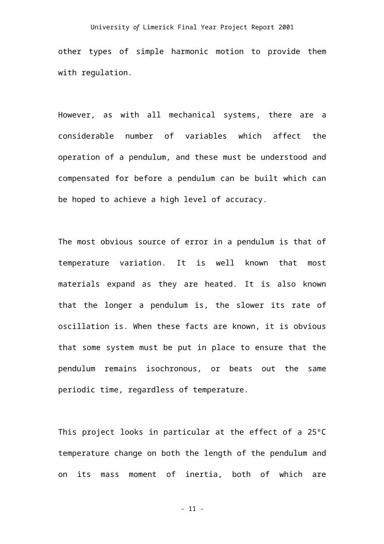
even today, mechanical clocks rely on pendulums or other types of simple harmonic
motion to provide them with regulation.
However, as with all mechanical systems, there are a considerable number of
variables which affect the operation of a pendulum, and these must be understood and
compensated for before a pendulum can be built which can be hoped to achieve a high
level of accuracy.
- 7 -

University of Limerick Final Year Project Report 2001
The most obvious source of error in a pendulum is that of temperature variation. It is
well known that most materials expand as they are heated. It is also known that the
longer a pendulum is, the slower its rate of oscillation is. When these facts are known,
it is obvious that some system must be put in place to ensure that the pendulum
remains isochronous, or beats out the same periodic time, regardless of temperature.
This project looks in particular at the effect of a 25ºC temperature change on both the
length of the pendulum and on its mass moment of inertia, both of which are
properties which will change with temperature. A solid modelling parametric CAD
program called ProEngineer is used for the mass property calculations, as it can deal
quite easily with the awkward shapes of the components of the pendulum.
The ProMechanica Finite Element Analysis software was also used to analyse the
interaction of four connected parts of the pendulum. These were made from different
materials, resulting in a complex contact stress problem, which can be solved
relatively easily using Finite Element Analysis. This problem would be extremely
difficult to solve satisfactorily using standard analytical methods because it would
require assumptions to be made to simplify the model.
The second aspect of this project was to design and build an uncompensated
pendulum, which can be used in experiments to measure the effect of a temperature
change on the pendulum.
The third aspect of the project was to investigate the effect of the mass moment of
inertia on the behaviour of the test pendulum as the temperature changed.
- 8 -

University of Limerick Final Year Project Report 2001
2.0 BACKGROUND THEORY
2.1 Moments
A moment is the term used to describe a turning force or torque. It is calculated by
multiplying the linear force applied by its perpendicular distance from the point about
which the moment is to be calculated[6].
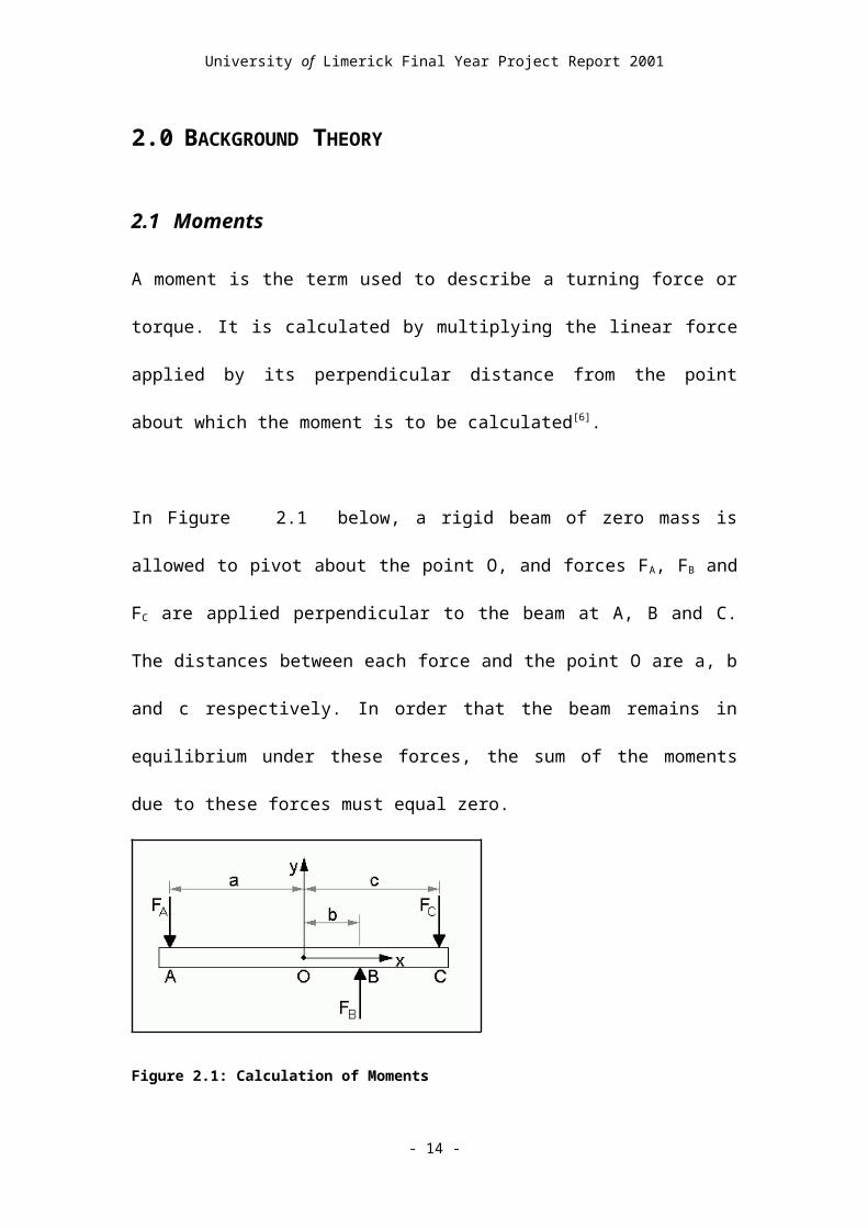
In Figure 2.1 below, a rigid beam of zero mass is allowed to pivot about the point O,
and forces FA, FB and FC are applied perpendicular to the beam at A, B and C. The
distances between each force and the point O are a, b and c respectively. In order that
the beam remains in equilibrium under these forces, the sum of the moments due to
these forces must equal zero.
Figure 2.1: Calculation of Moments
To calculate the moments due to the forces, each force is multiplied by its
perpendicular distance from the pivot O. It can be seen that the effect of the forces FA
and FB will be to turn the beam in an anticlockwise direction and the effect of the
force FC is to turn the beam clockwise. In order to differentiate mathematically
between clockwise and anticlockwise moments it is convenient to set the point O as
the origin for a co-ordinate system.
- 9 -

University of Limerick Final Year Project Report 2001
This results in the distance a being negative as it is on the negative side of the x axis,
while b and c are positive. The same procedure is followed for the forces, making FB
positive as it acts in the positive y direction, while FA and FC are both negative. The
overall effect of this is that anticlockwise moments are positive while clockwise
moments are negative.
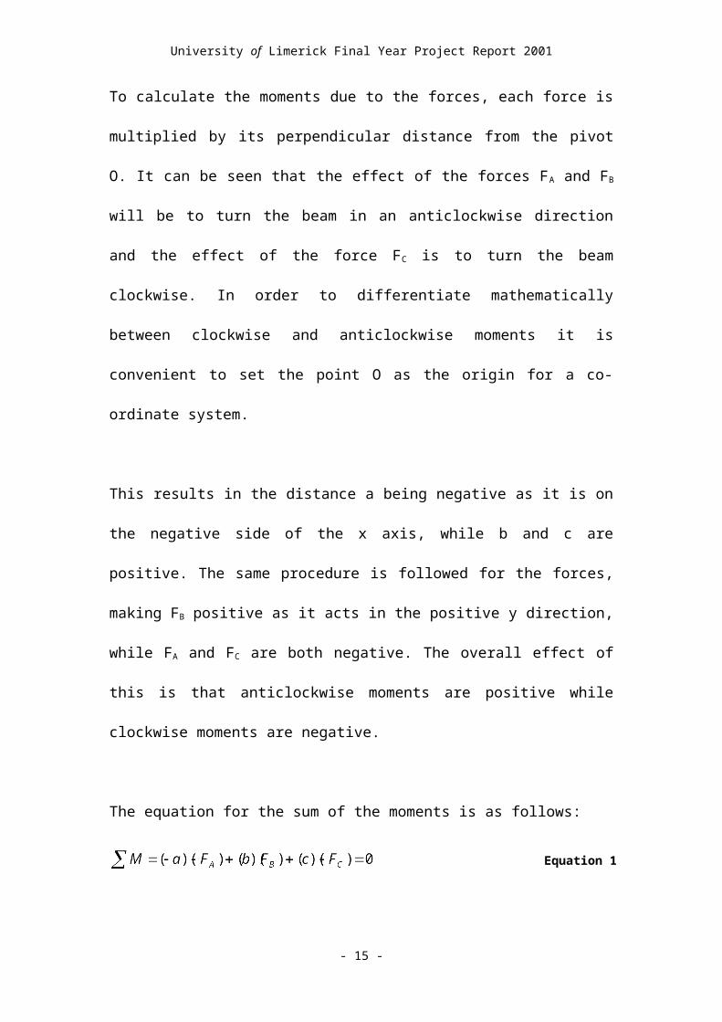
The equation for the sum of the moments is as follows:
Equation 1
2.2 Centre of Gravity
The centre of gravity of a body is the point through which gravity causes its weight to
act, regardless of the orientation of the body. The centre of gravity allows irregularly
shaped bodies to be replaced by point masses once it is known where the centre of
gravity is, and therefore where to put the mass. In order for a body to be in
equilibrium, the sum of the moments exerted by the forces acting on the body
including gravity and the net force acting on the body must equal zero. If this is not
the case, the body will accelerate, either in a linear or angular fashion, resulting in a
dynamics problem. In order to model this behaviour, the mass moment of inertia must
be known also. This is covered in Section 2.4.
- 10 -
University of Limerick Final Year Project Report 2001
The centre of gravity for a body of arbitrary dimensions can be determined
experimentally by suspending it on a string A from three different points of the body.
Since the string supplies the only force supporting the body and the body is in
equilibrium, the imaginary line made by the string through the body at each point
must pass through the
body's centre of
gravity. Where the
three lines cross,
therefore, is the centre
of gravity of the body.
Figure 2.2.1: Experimentally Determining the Centre of Gravity of a Body
In order to mathematically calculate the centre of gravity, consider a body of mass m
and weight mg = W. It is divided into an infinite
number of smaller masses, each of mass dm. The
force of gravity causes all of these masses to exert a
force dm·g = dW in the -y direction Relative to the
co-ordinate system in Figure 2.2.2.
Figure 2.2.2: Theoretical Calculation of the Centre of Gravity
Summing the moments exerted by each dW about each axis using integration gives the
moment exerted by the whole body about that axis. This is equal to the moment the
total mass will exert through its centre of gravity about the axis. When the centre of
- 11 -
University of Limerick Final Year Project Report 2001
gravity is assumed to be a distance from the x axis, from the y axis and from
the z axis the following equations can be derived:
Equations 2
These can also be expressed as
Equations 3
If a completely exact calculation of the centre of gravity is required, it should be noted
that gravity acts towards the centre of the earth, and therefore gravitational forces are
not parallel as assumed previously. Also, gravitational force varies with the inverse
square of the distance moved from the centre of the Earth, therefore the masses dm
positioned further away from the centre of the Earth will be multiplied by a smaller
value of g than masses nearer the Earth's centre.
This means that the position of the centre of gravity will change depending on the
orientation of a body. However, since the parts being analysed in this project are
- 12 -

University of Limerick Final Year Project Report 2001
extremely small with respect to the size of the Earth, the assumptions made here are
acceptable[6].
2.3 The Difference Between the Centre of Gravity and the
Centroid
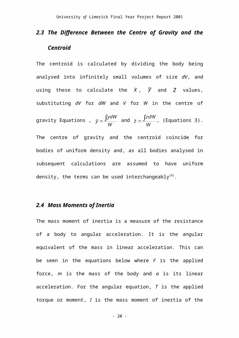
The centroid is calculated by dividing the body being analysed into infinitely small
volumes of size dV, and using these to calculate the , and values, substituting dV
for dW and V for W in the centre of gravity Equations , and ,
(Equations 3). The centre of gravity and the centroid coincide for bodies of uniform
density and, as all bodies analysed in subsequent calculations are assumed to have
uniform density, the terms can be used interchangeably[6].
2.4 Mass Moments of Inertia
The mass moment of inertia is a measure of the resistance of a body to angular
acceleration. It is the angular equivalent of the mass in linear acceleration. This can be
seen in the equations below where F is the applied force, m is the mass of the body
and a is its linear acceleration. For the angular equation, T is the applied torque or
moment, I is the mass moment of inertia of the body and (alpha) is its angular
acceleration. The angular acceleration can also be written as or .
Equation 4
Equation 5
- 13 -
University of Limerick Final Year Project Report 2001
The calculation of the mass moment of inertia is similar to the calculation of the
centre of gravity in that it involves dividing the body to be analysed into an infinite
number of smaller masses and using integration to calculate the total effect of these
masses.
Figure 2.4.3: Calculation of Moment of Inertia
Consider the body in Figure 2.4.3. It is being accelerated at the rate of rad/s2 about
the axis O-O. This means that at any instant the point P is accelerating linearly at a
rate of m/s2. The mass of the infinitesimally small part of the body at point P is
dm. When these values are substituted into the linear acceleration equation maF
(Equation 4), the resulting equation for any mass dm is:
Equation 6
Since Moment or Torque is force times distance;
Equation 7
- 14 -
University of Limerick Final Year Project Report 2001
Comparing this with IT (Equation 5) gives:
Equation 8
To calculate the moment of inertia for the whole body, all the dm values must be
added together using integration, therefore the mass moment of inertia about the axis
O-O is[7]:
Equation 9
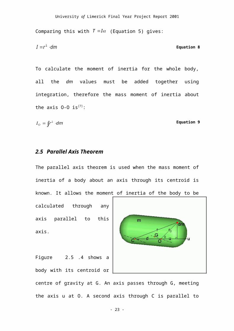
2.5 Parallel Axis Theorem
The parallel axis theorem is used when the mass moment of inertia of a body about an
axis through its centroid is known. It allows the moment of inertia of the body to be
calculated through any axis parallel to this axis.
Figure 2.5.4 shows a body with its
centroid or centre of gravity at G. An
axis passes through G, meeting the
axis u at O. A second axis through C is
parallel to this axis. The mass moment
of Inertia of the body about G is .
Figure 2.5.4: The Parallel Axis Theorem
- 15 -
University of Limerick Final Year Project Report 2001
To fill values into the integral for the new axis, the distance r must be calculated. The
cosine rule ( ) is used to calculate this value as follows:
Equation 10
Equation 11
From Equation 11, , the second term is , and the third term equals
zero. The reason for this is that since the axis through O also passes through G, the
centre of gravity, the average value of u when the masses dm for the whole body are
added together will equal zero. This gives the Parallel Axis Theorem result[7]:
Equation 12
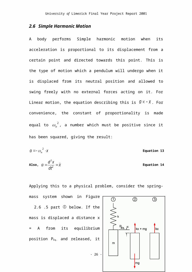
2.6 Simple Harmonic Motion
A body performs Simple harmonic motion when its acceleration is proportional to its
displacement from a certain point and directed towards this point. This is the type of
motion which a pendulum will undergo when it is displaced from its neutral position
and allowed to swing freely with no external forces acting on it. For Linear motion,
the equation describing this is . For convenience, the constant of
proportionality is made equal to , a number which must be positive since it has
been squared, giving the result:
Equation 13
- 16 -

University of Limerick Final Year Project Report 2001
Also, Equation 14
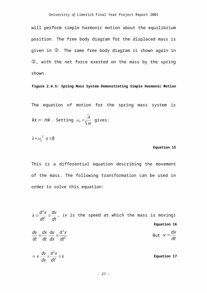
Applying this to a physical problem, consider the spring-mass system shown in Figure
2.6.5 part below. If the mass is displaced a distance x = A from its equilibrium
position PEq. and released, it will perform
simple harmonic motion about the
equilibrium position. The free body diagram
for the displaced mass is given in . The
same free body diagram is shown again in
, with the net force exerted on the mass by
the spring shown.
Figure 2.6.5: Spring Mass System Demonstrating Simple Harmonic Motion
The equation of motion for the spring mass system is . Setting
gives:
Equation 15
This is a differential equation describing the movement of the mass. The following
transformation can be used in order to solve this equation:
, (v is the speed at which the mass is moving) Equation 16
But
- 17 -

University of Limerick Final Year Project Report 2001
Equation 17
Substituting this into gives:
Solving gives:
, Where K is a constant of integration.
Equation 18
For all simple harmonic motion, v = 0 when x = A, where A is the amplitude of the
oscillation and v is the speed of the particle. Substituting these conditions into
Equation 18. gives , giving the overall equation:
Equation 19
Equation 20
But since v = , the following integral can be derived:
Equation 21
Solving gives:
, where is a second constant of Integration.
Equation 22
- 18 -

University of Limerick Final Year Project Report 2001
This equation is for a sine wave of amplitude A metres, with a circular frequency of
radians per second, and a phase angle of radians. This equation will model
undamped linear simple harmonic motion for all cases, provided the correct initial
conditions are substituted into the equation[8].
2.7 Modelling the Behaviour of a Simple Pendulum
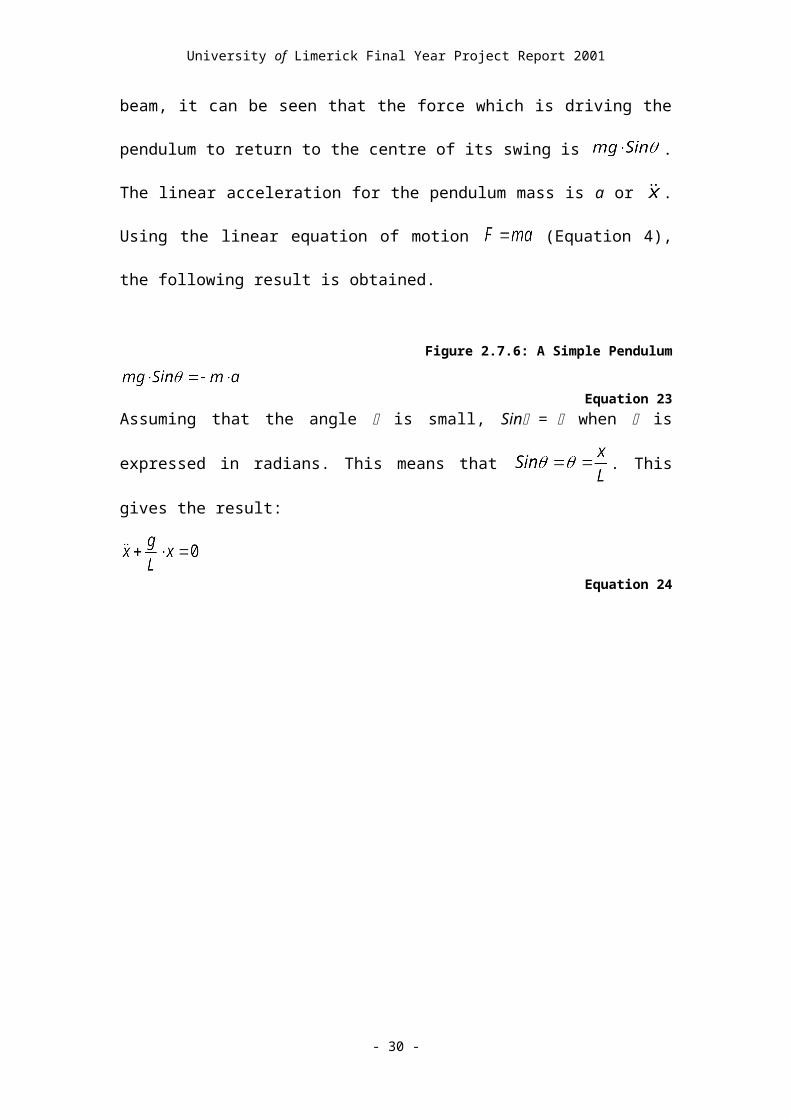
A simple pendulum consists of a point mass m at the end of a rigid massless beam of
length L. It is displaced a distance x from its initial position and allowed to oscillate as
shown in Figure 2.7.6. Splitting the force due to the
point mass into its components perpendicular and
parallel to the beam, it can be seen that the force
which is driving the pendulum to return to the centre
of its swing is . The linear acceleration for
the pendulum mass is a or . Using the linear
equation of motion (Equation 4), the
following result is obtained.
Figure 2.7.6: A Simple Pendulum
Equation 23Assuming that the angle is small, Sin = when is expressed in radians. This
means that . This gives the result:
Equation 24
- 19 -
University of Limerick Final Year Project Report 2001
Comparing Equation 24 to (Equation 15) gives:
Rad/s
From this, the periodic time is calculated using the formula giving:
Seconds
Equation 25
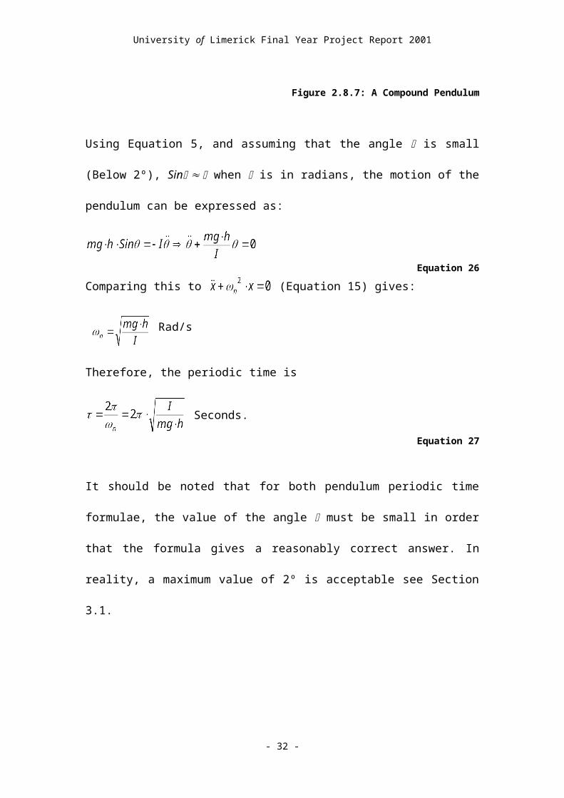
2.8 Modelling the Behaviour of a Compound Pendulum
A compound pendulum not only has mass, but also has a moment of inertia. Any
pendulum which exists in three dimensions must be analysed as a compound
pendulum, using the formula (Equation 5). I
is defined as the moment of inertia of the compound
pendulum about its pivot axis.
The compound pendulum analysis is very similar to
that for a simple pendulum. However, the
compound pendulum analysis equates torque values
rather than force values.
Figure 2.8.7: A Compound Pendulum
Using Equation 5, and assuming that the angle is small (Below 2º), Sin when
is in radians, the motion of the pendulum can be expressed as:
Equation 26Comparing this to (Equation 15) gives:
- 20 -

University of Limerick Final Year Project Report 2001
Rad/s
Therefore, the periodic time is
Seconds.
Equation 27
It should be noted that for both pendulum periodic time formulae, the value of the
angle must be small in order that the formula gives a reasonably correct answer. In
reality, a maximum value of 2º is acceptable see Section 3.1.
2.9 Coefficient of Thermal Expansion
All materials experience slight dimensional changes when they are heated. The
coefficient of thermal expansion is a way of quantifying this change. The coefficient
of thermal expansion for a particular material is defined as the change in length of a
one unit long bar of this material after it undergoes a temperature change of 1ºC.
The formula used to calculate this change is shown below:
Equation 28
Where LF is the new length of the part, LI is the initial length, T is the temperature
change and c is the coefficient of thermal expansion.
- 21 -

University of Limerick Final Year Project Report 2001
2.10Compensation Calculations
In the diagram of the compensated pendulum below, L1 and L2 are the lengths of the
two steel parts of the pendulum. Since these will behave the same way as a single
steel rod of the same total length, the total length of the steel parts is:
Equation 29
It is assumed that the centre of gravity of the pendulum is
the same as the centre of gravity of the Bob. It is for this
reason that the length LG must remain constant in order
for the pendulum to be compensated.
The periodic time of the pendulum is designed to be 1.5
Seconds. Using the simple pendulum periodic time
formula, Equation 27, LG is calculated to be:
Figure 2.10.8: Compensated Pendulum
Equation 30
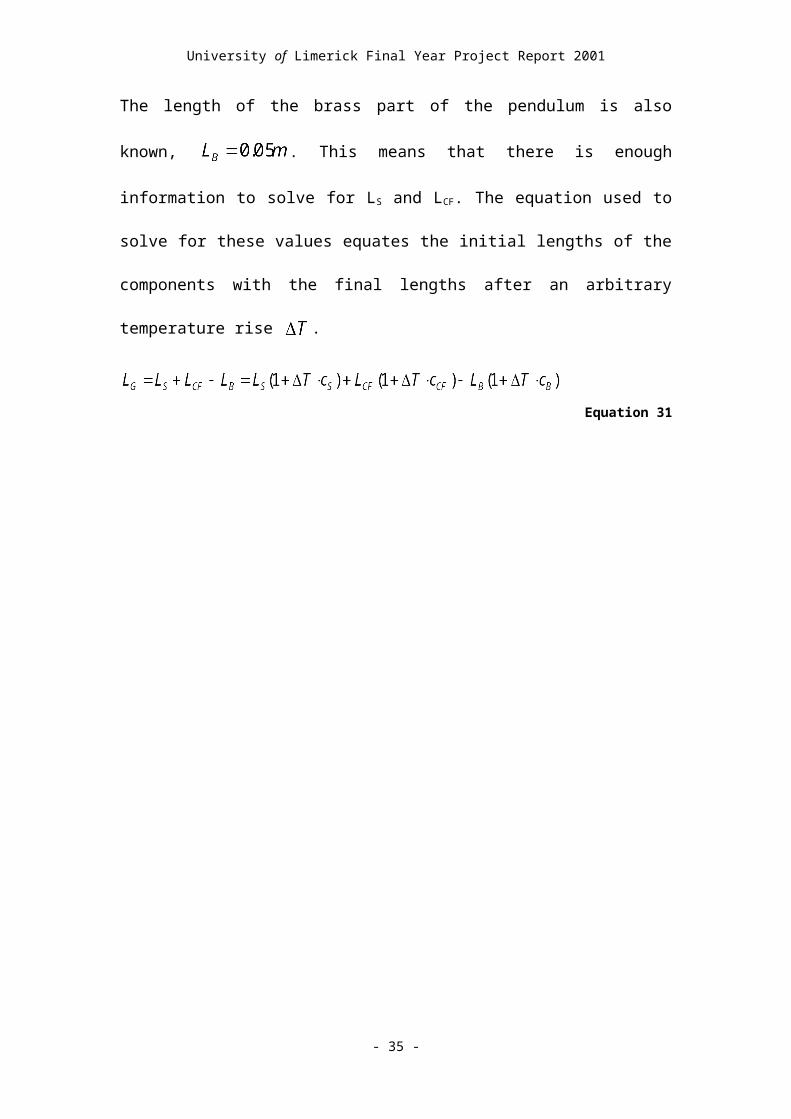
The length of the brass part of the pendulum is also known, . This means
that there is enough information to solve for LS and LCF. The equation used to solve
for these values equates the initial lengths of the components with the final lengths
after an arbitrary temperature rise .
Equation 31
- 22 -
University of Limerick Final Year Project Report 2001
This simplifies to
Equation 32
Substituting (Derived from Equation 31), gives the solution for the
length of the Carbon Fibre rod:
Equation 33
This gives LS = 0.1218m [11].
- 23 -

University of Limerick Final Year Project Report 2001
3.0 ERRORS IN MECHANICAL CLOCKS
3.1 Circular Error
The first thing which must be said about pendulums is that they do not actually
perform simple harmonic motion. As has been shown previously in this report, in
deriving the equations of motion for the pendulum see Section 2.7, it is assumed that
the Sine of the angle through which the pendulum is displaced from the centre is
equal to the angle in radians. This is quite acceptable in most cases, but in the use of
pendulums for precision timekeeping, it can be a major source of error.
Figure 3.1.9: Circular Error Graph
The graph above shows how the error climbs exponentially as the half arc angle
rises past 2º or so. It is for this reason that the pendulum has to move through exactly
the same arc angle for each oscillation, or else it will not remain isochronous. As the
- 24 -
University of Limerick Final Year Project Report 2001
arc angle rises, the periodic time of the pendulum will also increase, causing the clock
rate to decrease.
To compensate for circular error, the pendulum must be made to swing through a
cycloidal arc rather then in a circular arc. The effect of this is that as the pendulum
swings further from the centre of its arc, its effective length should drop, thereby
causing the rate of the clock to increase
until the pendulum returns to its design arc.
A means of doing this was invented by
John Harrison, a clockmaker in England in
the 1700’s, and is shown in Figure 3.1.10.
Figure 3.1.10: Circular Cheeks used to make the arc of the pendulum cycloidal
The adjusting screws and the empty slot on the centre line of the cheeks are for fitting
them onto a lathe in order to adjust the radius of the cheeks and in doing so, the
circular error of the pendulum. The usefulness of this adjustment will be seen later. It
should be noted that the aim of these cheeks is not to eradicate circular error, but to
adjust it.
3.2 What causes a Pendulum to Change Rate?
3.2.1 Environmental Conditions
In order for a pendulum to keep perfect time, it must be kept in a totally stable
environment. That is, the pressure, temperature, gravity and energy input to the
pendulum and energy losses from the pendulum must all remain exactly the same.
- 25 -
University of Limerick Final Year Project Report 2001
Many attempts have been made to do this, but in order to keep the environment stable,
the pendulum must be mounted on a completely rigid support, in a total vacuum, with
a constant energy driving it. It must also have a frictionless suspension and not be
exposed to changes in temperature or to light, which also adds energy to the
pendulum.
Even gravitational effects caused by the moon and the sun acting on the Earth (The
same force which causes the tides), have to be isolated in order to ensure a completely
isochronous pendulum. This makes the construction of an isolated pendulum highly
impractical and expensive.
It should also be noted however, that even if these effects could all be isolated, the
inherent problems which cause the periodic time to deviate would still not be
eliminated. In fact, if a pendulum was designed to operate in total isolation and some
small outside effect such as a stray vibration caused the pendulum’s arc to change,
there would be no restoring force to bring it back to its design conditions. Because of
this, the outside influence would cause the pendulum to compound errors instead of
losing them over time.
It is for this reason that clocks with pendulums designed to operate in highly
controlled environments can often be as inaccurate as those which are left to operate
in normal changing conditions.
- 26 -
University of Limerick Final Year Project Report 2001
The changes in conditions to which a pendulum will be exposed are as follows:
3.2.2 Temperature Change
Changes in temperature will cause the parts of the pendulum to expand or contract.
The effect the change in temperature has on the pendulum shape is the subject under
investigation in this project. The length of the pendulum must be exactly regulated as
in order to maintain an accuracy of 1 second in 100 days, which has been the target
accuracy for mechanical regulators since the 1700’s, the length of the pendulum must
not change by more than 230nm[1].
The temperature also affects the density and therefore the viscosity of the air through
which the pendulum travels, reducing the viscosity as the temperature rises. Also, if
oil is used in the clock mechanism, this will change viscosity and affect the motion of
the pendulum too. It is partly for this reason that virtually all regulators run without
oil.
3.2.3 Pressure
An increase in pressure will cause the density of the air to rise, increasing the air
resistance on the pendulum. This causes the arc of the pendulum to drop, and since it
takes more energy to push it through the thicker air, the clock rate will also drop. Air
pressure changes also increase or decrease the weight of the pendulum by a small
amount, as the air surrounding the pendulum will act to float it, thereby reducing the
restoring force on the pendulum as in Section 2.7. This also causes the rate
of the clock to drop.
- 27 -

University of Limerick Final Year Project Report 2001
3.2.4 Gravity
The force exerted due to gravity changes with distance from the centre of the Earth, as
well as with the relative positions of the sun and moon. However, assuming the clock
is left in the one place, the cyclic changes due to the sun and moon are never enough
to cause an error of 1 second in 100 days. An increase in gravitational force causes the
clock to run faster, with a decrease having the opposite effect (See Section 2.7).
3.2.5 Energy input
If a pendulum is set swinging in air, without an outside energy source to drive it, it
will eventually stop due to air and mechanical friction. A graph of this can be seen in
Figure 5.3.19 from the experimental work in this project.
Increasing the energy driving the pendulum will cause the pendulum to swing through
a wider arc. From the previous discussion on circular error in section 3.1, this should
cause the clock rate to drop. However, the actual effect of an increase in energy input
on most pendulums is to make the clock run faster, as the escapement has too much
control over the pendulum motion.
This effect can be minimised by making the crutch, which drives the pendulum as in
Figure 9.1.26, as short as possible in relation to the pendulum length, increasing the
mass of the bob or reducing the recoil forces from the escapement. Another method is
to increase the arc angle of the pendulum and use circular error to make the clock run
more slowly, while the escapement is trying to drive the clock more quickly, thus
making both errors cancel eachother out. It is this method of dealing with errors which
- 28 -

University of Limerick Final Year Project Report 2001
has been investigated as a solution to the problem of the effect the environment has on
pendulums.
If oil is used in the clock mechanism, as it collects grit and dust, more energy will be
required to keep the clock running. This also means that a clock using oil will have to
be recalibrated every time it is cleaned, as well as while it is running to compensate
for changes in the oil. This is the second reason oiled mechanisms are not used.
3.2.6 Conclusion
What is needed is a system which uses its environment as a source of self regulation,
rather than a system which must be isolated from the environment to work properly.
Such a system was developed, built and refined by a Yorkshire man named John
Harrison (1693-1776) as a result of devoting over sixty years of his life to the pursuit
of more accurate timekeeping during the 1700's.
Harrison's system uses the resistance of the pendulum as it moves through the air as a
sink for energy applied to the pendulum by the escapement mechanism. To do this, he
used a pendulum arc of 12º, contrary to accepted pendulum theory (Section 2.7).
However, once the effect of circular error can be controlled, as in Figure 3.1.10, this
has several benefits in terms of the precision of the clock.
The reason this arrangement improves accuracy is that as the pendulum swings
through a large arc, it has far more kinetic energy than a small arc pendulum of the
same mass, but it also loses more energy through air friction than an equivalent small
arc pendulum too. It is known that a light pendulum which has a large energy
- 29 -
University of Limerick Final Year Project Report 2001
throughput will remember a disturbance for far less time than a heavy pendulum with
a short arc, and this is the part of the reason Harrison used a large arc in his regulators.
The large arc also causes more air to wash over the pendulum, allowing it to reach
thermal equilibrium more quickly, making the temperature compensation in the
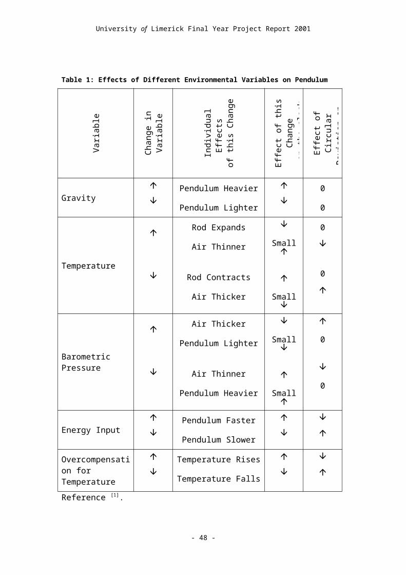
pendulum more effective. As can be seen in Table 1, circular error will counteract the
effects of all the variables previously discussed, except for temperature fluctuations. It
is for this reason that the temperature compensation is necessary.
- 30 -

University of Limerick Final Year Project Report 2001
Table 1: Effects of Different Environmental Variables on Pendulum
Var
iabl
e
Cha
nge
in V
aria
ble
Indi
vidu
al E
ffec
ts
of th
is C
hang
e
Effe
ct o
f thi
s Cha
nge
on
the
cloc
k R
ate
Effe
ct o
f Circ
ular
D
evia
tion
on
Clo
ck R
ate
Gravity
Pendulum Heavier
Pendulum Lighter
0
0
Temperature
Rod Expands
Air Thinner
Rod Contracts
Air Thicker
Small
Small
0
0
Barometric Pressure
Air Thicker
Pendulum Lighter
Air Thinner
Pendulum Heavier
Small
Small
0
0
Energy Input
Pendulum Faster
Pendulum Slower
Overcompensation for Temperature
Temperature Rises
Temperature Falls
Reference [1].
- 31 -
University of Limerick Final Year Project Report 2001
4.0 EXPERIMENTAL WORK
4.1 Introduction and Aims
The purpose of the experimental work in this project was to examine the effects of
temperature changes on the timekeeping of a pendulum. It was originally planned that
the compensated pendulum designed by Dr. Richard Stephen would be used, but no
convenient source for the carbon fibre rod used in this pendulum could be found.
It is also likely that any carbon fibre rod sourced would have a different coefficient of
expansion to the one used in the compensated pendulum analysed, and since there was
no way of measuring the coefficient of thermal expansion available, this would make
the construction of a correctly compensated pendulum unfeasible.
The staff in the engineering workshops were reluctant to commit to making the
pendulum to the precision needed in order that its compensation would work
correctly, as there were many other projects in progress at the same time, and
constructing the pendulum would have taken up a disproportionate amount of
workshop time.
If the compensated pendulum was used, there would also have been a problem with
measuring the effect of the temperature change, as it should theoretically be zero. The
compensated pendulum uses a spring suspension, making it far more susceptible to
higher modes of vibration in the pendulum itself, as well as twisting, all of which
would add to the experimental error, rendering any measurements made unreliable at
best. In fact, in order to get reliable results from experiments using this pendulum, it
- 32 -

University of Limerick Final Year Project Report 2001
would be necessary to fit an escapement mechanism to it and measure the periodic
time over several days, while the temperature was also regulated.
It was concluded from this that it would be far more convenient if a pendulum test rig
was designed and built specifically for the experiments required. The criteria for this
design are in Section 4.2.
The aims of the experiments were, first of all, to establish the need for temperature
compensation, and secondly to compare the theoretically calculated periodic time of
the pendulum with the actual measured periodic time and see whether the measured
change due to temperature was the same as the theoretically calculated change. The
effect of air resistance on the pendulum was also investigated as this is the force
which causes the pendulum arc to drop during the experiments performed.
In order to perform the experiments necessary, a pendulum of known dimensions and
material was needed, as well as a means of measuring the periodic time and regulating
the temperature at which the pendulum was held. The following sections describe the
experimental equipment and procedure used for the experiments.
4.2 Design Criteria For Test Pendulum
The most important aspect of the pendulum design was that it should fit into the oven
to which it was allocated for the experimental work. If there was no way to regulate
the temperature to which the pendulum is exposed, the experiments could not have
been performed. This criterion was the force that drove the limiting dimensions for
the pendulum length and the size of the supporting frame. The approximate
- 33 -

University of Limerick Final Year Project Report 2001
dimensions of the inside of the oven were 690mm high x 590mm wide x 350mm
Deep.
The test pendulum was designed to be easy to build. This allowed it to be constructed
using basic lathes, a milling machine and a pillar drill. All this equipment was readily
available and the simple design allowed the pendulum to be built over a two-week
period. This design would also have allowed the pendulum to be made by students if
the machine room staff were too busy.
The simple shapes of the parts from which the pendulum is made allow easy mass
moment of area calculations to be performed.
The parts of the pendulum are also all made from the same material. This allows it to
be analysed as a solid assembly, rather than as separate parts as would be necessary
for pendulums using a mix of materials, such as the compensated pendulum.
The pendulum was designed with robustness in mind, as it was known that it would
have to be transported from where it was made to set up the experimental equipment
as well as for the experiments to be performed. Also, since the area where the
pendulum was to be stored was left open most of the time, there was always the
possibility that it would be tampered with. This is part of the reason that the
calibration procedure for the pendulum was made as simple as possible, it was also
done to remove changes in calibration as a source of error since the pendulum
calibration can be checked quickly every time it is used.
- 34 -
University of Limerick Final Year Project Report 2001
The main dimensions of the pendulum can be easily measured and confirmed. This
allows the correct values to be put into the theoretical calculations for the pendulum
period.
A proximity switch was chosen to measure the period of the experimental pendulum
for the following reasons;
It was easy to source a proximity switch, as there was a supply of them readily
available in the University.
The proximity switch used is designed to operate at temperatures up to 70°C
(Farnell Catalogue), which is well within the temperature range of the planned
experiments.
The rise time for the signal from the switch was measured using a HP
Oscilloscope with a clock speed of 150MHz, giving a sub 7ns resolution, to be
under 1.74 microseconds. This means that the switch reaction time will not
have a significant effect on the measurements taken using the switch.
Steel was the material chosen for the pendulum, so a proximity switch is the
ideal method to use to monitor its movement, as the pendulum rod can be
detected directly. This means that no modifications have to be made to the rod
to allow the period to be measured.
The cylindrical pendulum rod allows the proximity switch to be highly
selective in its registering of the rod passing, as the switch will only pick up
the nearest edge of the rod instead of the whole width of it. The sensitivity can
be adjusted by sliding the pendulum forwards or backwards on the knife-edge.
- 35 -
University of Limerick Final Year Project Report 2001
Since there was nothing to drive the pendulum, the emphasis of the design was to
remove as much friction as possible from the system because, during the course of the
experiment, the arc through which the pendulum swings reduces, causing the periodic
time of the pendulum to fall also. A knife-edge pendulum suspension was chosen as
the easiest way to do this. It is not only easy to make and uses very little energy in
operation, but it is also far less susceptible to higher modes of vibration such as
twisting and forwards and backwards vibration, which cause considerable problems if
a suspension spring is used.
4.3 Equipment Used
K Type Thermocouple Amplifier (See Section 9.3 for calibration details)
Blackstar Apollo 10 Universal Counter Timer with 2MHz and 100MHz clocks.
IMEX NE 481 Dual Voltage/Current Supply
Potential Divider Circuit with Diode to Prevent Back e.m.f.
Schönbook Electronic PNP, 10 to 35V DC Proximity Switch, Serial No. ILII214
Gallenkamp size three Oven BS. Model CV-160, 13A 250V. Approximate Internal
Dimensions: 690H x 590W x 350D. Thermostat Calibrated to ±5º.
Intel Pentium 133 with 48Mb RAM. Running LabVIEW Version 5.1.1 Software and
with the PC-1200AI LabVIEW Interface Card Installed.
Radionics Heat gun 500S 1500W
HP Oscilloscope: Model Number: HP54602B with 150MHz Clock (Used for testing
the proximity switch).
- 36 -
University of Limerick Final Year Project Report 2001
4.4 Equipment Set up
The equipment was set up as in Figure 4.4.11, Figure 4.4.12, Figure 4.4.13 and Figure
4.4.14.
Figure 4.4.11: The Experimental Pendulum set up in the Oven.
Figure 4.4.12: Close-up of Pendulum Bob, showing Proximity Switch, threaded bar and thermocouple.
Figure 4.4.13: Equipment used to log Temperature and Periodic Time.
Figure 4.4.14: Power Supply, Timer/Counter, Thermocouple Reader and LabVIEW Connector Board.
- 37 -

University of Limerick Final Year Project Report 2001
The wiring diagram for the electronic connections is shown in Figure 4.4.15.
Figure 4.4.15: Wiring Diagram for Experimental Equipment.
4.5 Calibration Procedure for Test Pendulum
It was confirmed that the pendulum rig frame was
level by using a setsquare and spirit level to check
that the front left leg was level and the left hand
upright of the frame was vertical. The levelling
procedure is shown in Figure 4.5.16. Pieces of
cardboard were inserted under the legs to level the
frame if it was not level to start with. After each
subsequent stage in the calibration, the pendulum was
again confirmed to be level.
Figure 4.5.16: Confirming that the pendulum frame is Level.
- 38 -

University of Limerick Final Year Project Report 2001
Next the 20V supply to the proximity switch was turned on and it was confirmed that
the proximity switch registered the pendulum rod passing its tip. If the switch did not
operate, it was moved towards the pendulum rod by loosening the nuts holding it to
the plate adjusting it forwards and tightening the nuts again. Fine-tuning can then be
performed by sliding the pendulum towards or away from the switch on its knife-edge
mounting.
The centring of the switch was also checked by ensuring that when the pendulum
came to rest in the centre of its swing, the switch was activated. A visual check was
also performed to ensure that the pendulum spent approximately the same amount of
time at each side of the proximity switch when it was sent through a small arc. If this
was not the case, the centring of the proximity switch was adjusted by gently tapping
the plate it is mounted in, thus causing it to move slightly in the required direction.
The play between the holes drilled for the bolts in the plate and the bolts themselves
allows this movement to take place.
As has been demonstrated previously in Section 2.7, keeping the half arc of the
pendulum below 2° will almost eliminate the effects of circular error on the
pendulum, thus rendering it effectively isochronous during the course of the
experiment. The arc angle can be measured using a ruler fitted to the pendulum frame
to measure the displacement of the tip of the pendulum rod.
To calculate the displacement of the end of the pendulum rod required to keep the
pendulum half arc angle under 2°, basic trigonometry can be used as follows:
- 39 -

University of Limerick Final Year Project Report 2001
Actual Rod Length Measured from knife-edge pivot to free end: 0.5739 m
Half Arc Angle required 2°.
Displacement of end of rod with 2° half arc angle:
= 0.5739 Sin (2°) = 0.020028821m. Equation 34
Therefore, a displacement of 20mm will give a half arc angle under 2°.
The threaded rod at the left hand side of the pendulum frame was adjusted to prevent
the pendulum from moving more than 20mm from its central position, which was
measured on the ruler at the base of the pendulum. The threaded rod makes the arc
angle for the experiments repeatable.
4.6 Experimental Procedure
The following experiments were performed on Saturday 24th February between 12:00
and 20:00.
The equipment was set up and calibrated as described in sections 4.4 and 4.5, with the
pendulum rig installed in the oven. The thermocouple was positioned to measure the
temperature of the air near the pendulum as shown in Figure 4.4.12.
The oven was then turned on and set to the temperature required. (As the oven is
regulated to a minimum of 40°C, the first tests were performed at room temperature,
without turning the oven on.)
The pendulum was then made to oscillate by moving the pendulum to the left until the
bob touched the tip of the threaded rod. The pendulum was then released and allowed
- 40 -
University of Limerick Final Year Project Report 2001
to swing freely. It was visually examined for excessive forward and reverse vibration
and the starting procedure was repeated if this was the case. The oven door was then
closed.
The counter/timer and the LabVIEW temperature logging program were started
simultaneously. The temperature logger was set to log the temperature every 5
seconds for a 15 minute time period.
The average periodic time reading calculated by the counter timer for every 10 cycles
was recorded in a text file on the computer while the LabVIEW program was logging
the temperature.
When the temperature logger indicated that the time for the experiment had elapsed, a
last periodic time reading was taken, and the time and temperature log files were
saved to the hard disk of the computer. This completes one set of experimental
readings. This procedure was repeated twice more at room temperature.
The oven was then set to a temperature equal to the average temperature recorded
during the previous readings plus 25ºC, i.e. 42ºC. A 30-minute time period was left to
allow the air in the oven and the parts of the pendulum to reach thermal equilibrium.
The temperature in the oven was measured using the thermocouple and temperature-
logging program, over a period of 1 minute to confirm that the temperature in the
oven was stable to ±5ºC prior to beginning the elevated temperature experiments.
- 41 -

University of Limerick Final Year Project Report 2001
While oven was running, the door was opened and the pendulum oscillation started.
The oven door was gently closed as soon as it had been visually confirmed that there
were no significant forwards and backwards vibrations in the pendulum.
After waiting for 1 minute to allow the air temperature in the oven to stabilise, the
oven was turned off. A time of 30 seconds was waited for, to allow the oven’s fan to
stop and the air currents in the oven to die out.
The timer/counter and the temperature logger were started simultaneously at the end
of the 30 seconds. The temperature logger was set to log the temperature every 5
seconds for 14 minutes. The reason for the change in time is that the pendulum will
have been oscillating for 1.5 minutes before any readings are taken in the elevated
temperature tests, so in order to compare like readings, 1.5 minutes are added to every
time reading taken for the elevated temperature tests as can be seen in the results
graphed in Figure 5.1.17.
The average for every 10 periods was recorded from the timer counter as before, with
the record of periodic time continuing until the temperature logger indicated that the
time for the experiment had elapsed.
This procedure was repeated twice more for the elevated temperature, recording the
average period measurement over every 10 samples, turning the oven on for 30
minutes between each experiment. The stability of the temperature was confirmed by
ensuring that the thermocouple reading remains within ±5°C for at least a minute
before starting a new experiment.
- 42 -
University of Limerick Final Year Project Report 2001
4.7 Further Test to Confirm Pendulum Properties
This test was performed on Wednesday 28 March 2001, between 15:00 and 16:30.
Since the readings taken in the previous experiment gave results which were clearly
inconsistent with the known behaviour of uncompensated pendulums, see Section 5.1,
a second test had to be performed, using a heat gun to heat the pendulum rod directly,
in order to confirm that it does expand as its temperature rises.
The pendulum was positioned in an open room and calibrated as in section 4.5. The
pendulum was started and left oscillating for 30 seconds to allow it to stabilise.
Periodic time readings were then taken for the pendulum over the next minute. The
ambient air temperature was measured during the experiment in order to get an
average value for the initial temperature of the pendulum.
The pendulum rod was then heated for 3 minutes using a heat gun, giving the rod an
estimated temperature of 50°C ± 10ºC, while the knife edge and pendulum bob were
only heated by conduction from the pendulum rod. After the 3 minutes were up, the
pendulum was started again, and readings for its periodic time were taken over the
next 2 minutes, after first allowing 30 seconds for it to stabilise.
The pendulum was then allowed to cool for 20 minutes and its periodic time was
measured over 1 minute, again after a 30 second delay for stabilisation.
- 43 -

University of Limerick Final Year Project Report 2001
5.0 RESULTS AND DISCUSSION
5.1 Experiments Involving the Oven
The results of the experiments using the oven are shown in the following graphs and
tables. The raw data from which the graphs were produced can be found in the
Appendix in Sections 9.20 and 9.21.
Figure 5.1.17 displays all the information collected during the course of the
experiments described in Section 4.6. As can be seen from the results, there is clearly
something wrong with the conditions under which this experiment was performed. As
an increase in periodic time was expected, when a decrease is what actually occurred.
It should also be noted that the periodic time measured was for the half period of the
pendulum, as the proximity switch will register the pendulum rod passing it twice for
every full oscillation of the pendulum.
The elevated temperature period readings also fluctuate enormously, indicating that
there is something causing the pendulum to deviate which was not present for the
room temperature readings. The only difference in conditions between the two sets of
experiments was that the oven had been turned on prior to the elevated temperature
readings being taken, causing air currents to be produced in the oven as it was fan
assisted.
Fluctuations in the temperature readings can also be seen for both high and low
temperature experiments, indicating that these fluctuations are not due to the oven, but
more likely due to the equipment used to measure the temperature.
- 44 -

University of Limerick Final Year Project Report 2001
The LabVIEW software or hardware is thought to be the reason for the temperature
measurement problem, as plugging a multimeter into the outlets from the
thermocouple amplifier results in a steady measurement, and since some readings
taken 5 seconds apart vary by 20ºC, it is not possible that these readings are correct.
However, when the obviously incorrect values have been removed from the data set,
the average temperatures calculated using the remaining readings should give an
adequate measurement of temperature for the purpose of this experiment.
Figure 5.1.17: Results of the Experiments performed using the oven (The Periodic time measured is half the actual Period)
- 45 -
University of Limerick Final Year Project Report 2001
Table 2: Summary of Experimental Results Compared with Theoretical and ProEngineer Calculations.
Tests at Room Temperature Average Temperature
Periodic times from
Experimental Results
Average Period(Sample is from 100 to 600 seconds in each Data Set)
Theoretical Results Calculated for a 25°C Temperature Change
Manual Calculation ProEngineer Calculation1 17.25°C 1413412.80 μs 1.413412797 s2 17.28°C 1413086.46 μs 1.413086458 s3 17.23°C 1413193.11 μs 1.413193114 s
Average 17.26°C 1413230.79 μs 1.413230789 s 1.405769274 s 1.407497449 s
Elevated Temperature Tests1 39.87°C 1412715.91 μs 1.412715908 s2 39.65°C 1412741.99 μs 1.41274199 s3 42.67°C 1412694.34 μs 1.412694336 s
Average 40.73°C 1412717.41 μs 1.412717411 s 1.405962554 s 1.40769097 s
Change 23.47°C -513.38 μs -0.000513378 s 0.00019328 s 0.000193521 s
% Change 136.045608 % -0.036326546 % -0.036326546 % 0.0137491 % 0.013749317 %
The average temperature readings were calculated after removing obviously incorrect Temperature readings i.e. Those under 14ºC for room
temperature and those under 35ºC for the high temperature readings. Between 8 and 16% of the temperatures read over the period of the test were
rejected in this way. It should be noted that in almost all cases, figures outside the tolerances given occurred singly, with it being unusual to have two
consecutive measurements rejected. The ProEngineer calculation is for a pendulum with the design dimensions. The manual calculation result is for a
pendulum of the same dimensions as the actual pendulum tested.
- 46 -

University of Limerick Final Year Project Report 2001
Table 2 shows, the compiled results comparing the experimental results at 17ºC and
41ºC with the theoretically calculated results using the moment of area formulae in
Section 9.2, as well as the results from the calculations performed by ProEngineer on
a CAD model of the pendulum.
Table 3: Comparison of Percentage Differences Between Results
Values Above Hatched Diagonal Boxes are for Room Temperature Results. Values below Diagonal are for Elevated Temperature Results.
% Deviation Experimental Manual ProEngineer
Experimental -0.527975709 % -0.405690316 %
Manual -0.478146393 % 0.122934457 %
ProEngineer -0.355799482 % 0.122934719 %
Table 3 compares the percentage errors between the different methods used to find the
periodic time of the pendulum. The correlation between the ProEngineer and the
manual calculations was expected to be good, though the ProEngineer model is for a
pendulum of exactly the design dimensions as given in Section 9.8, while the manual
calculations are for a pendulum of the same dimensions as the test pendulum
constructed.
ProEngineer is more accurate in its calculations, as it is dealing with the exact shape
of the pendulum, rather than the simplified assembly of regularly shaped parts which
was analysed using manual calculations in Section 9.3. However, the results from
ProEngineer correlate with the results from the manual calculations to 0.00686% if
the same dimensions are used for both sets of calculations, indicating that the
assumptions made in the manual calculations are acceptable.
- 47 -
University of Limerick Final Year Project Report 2001
5.2 Results from Experiments Involving the Independent
Heating of the Pendulum Rod
The periodic times measured when the pendulum rod was heated independently are
graphed in Figure 5.2.18. The ambient air temperature during these experiments was
21°C ± 1°C. The estimated temperature of the pendulum rod after it was heated for 3
minutes was 50°C ± 10°C, though the large tolerance indicates the low level of
confidence with which the reading was taken since the temperature was measured by
holding the thermocouple against the rod for several seconds.
However, this uncertainty is acceptable for the rod temperature measurement, as the
most important aspect of the experiment is that the rod was heated to a significantly
higher temperature than for the initial readings and not the value of the change. The
aim of this experiment was to confirm that the change in temperature had the correct
effect on the periodic time. These results cannot be interpreted as reliable readings
and were only taken to show that the trend is correct.
- 48 -
University of Limerick Final Year Project Report 2001
Figure 5.2.18: Results from Heating Pendulum Rod on its Own
It can be seen from Figure 5.2.18 that there is a clear increase in the periodic time of
the pendulum after the rod is heated. This effect is also shown to be temperature
related as, after the pendulum cooled, the periodic time returned to its initial value.
The reason consecutive periodic time readings vary is mostly due to air currents in the
room, as there was a noticeable deviation in the period after people opened the door to
enter or leave the room. The pendulum was completely exposed to the air currents in
the room for the duration of the experiment, but since there was no major change in
these currents while the experiment progressed, the temperature effect on the
pendulum could be measured.
- 49 -

University of Limerick Final Year Project Report 2001
5.3 The Modelling of the Periodic Time Decrease as the
Experiment Progressed
Figure 5.3.19: A best fit line modelling the change in the period of the pendulum averaged over three experiments as a logarithmic decrement.
The graph in Figure 5.3.19 shows a logarithmic best-fit line overlaid on averaged
values for the periodic time of the test pendulum. The period decays because, due to
air friction, the pendulum arc drops as the experiment progresses.
The Equation of the line, as well as its R² value, which is the correlation coefficient
for the line, are also shown on the graph. The nearer the R² value is to 1, the better the
points in the graph match the best-fit line.
Best-fit lines were also calculated for the same data, using linear, polynomial and
exponential approximations, but the best correlation was achieved using the
- 50 -

University of Limerick Final Year Project Report 2001
logarithmic line. This allows the conclusion that the pendulum period decays in a
logarithmic fashion to be reached from the experimental information gathered.
6.0 THE EFFECT OF THE CHANGING MASS MOMENT OF
INERTIA
The formulae for calculating the mass moment of inertia for the two component
shapes of the test pendulum (Appendix Section 9.2), indicate that a linear change in
temperature and therefore in the dimensions of the part, results in a second order
polynomial change in the mass moment of inertia.
However, when calculations for the test pendulum were repeated for several different
temperatures, and the mass moments of inertia graphed as in Figure 5.3.20, the actual
change in the mass moment of inertia for the pendulum looked to be linear. The
change in the periodic time of the pendulum also looked to be linear as in Figure
5.3.21.
- 51 -

University of Limerick Final Year Project Report 2001
Figure 5.3.20: Mass Moment of Inertia changes in the test Pendulum due to temperature changes.
Figure 5.3.21: Variation of Periodic Time with Temperature for the Test Pendulum
The reason for this linearity is due to the small size of the changes in the dimensions
of the pendulum. Using the formula for the mass moment of inertia of a cuboid, the
following results are obtained.
- 52 -

University of Limerick Final Year Project Report 2001
These calculations are based on the knife edge of the experimental pendulum, though
they work for the cylindrical portions and for the parallel axis theorem when it is
applied to get the mass moment of inertia about the pivot axis, as the changes in the
dimension values will be of the same order. Using the coefficient of thermal
expansion for steel, if there is a 10ºC temperature rise, the dimensions of the
pendulum will change by a factor of approximately .
From Section 9.2, for a cuboid. For the knife edge , giving the
result that for this part of the model at the initial temperature.
For each , the temperature is raised by 10ºC, giving the following results for Ip:
The value of , the difference between consecutive mass moment of inertia
calculations is , this gives:
From these results, it can be seen that the change in mass moment of inertia can be
divided into two parts. The first part is what shows on the graph, which is a linear
- 53 -

University of Limerick Final Year Project Report 2001
increase of between every value. The second part is a second order
increase, but in order for this to be as large as the linear part of the increase, the
temperature would have to rise by 100,000ºC, resulting in the non-linear change being
of magnitude .
The result of this is that the change in the periodic time of the pendulum will also be
effectively linear for the temperature range at which it was tested. From this it can be
concluded that the change in mass moment of inertia can be treated as a linear effect
for calculations involving temperature compensation in pendulums, unless very high
coefficients of expansion are involved. Therefore, a linear system of compensation is
adequate to deal with the effect of the mass moment of inertia change. This is most
likely the reason little research has been done into the effect the mass moment of
inertia change has on the behaviour of a pendulum, as the changes described in
Section 3.2 have been investigated because they have been isolated as definite sources
of error in the operation of actual clocks.
- 54 -

University of Limerick Final Year Project Report 2001
6.1 Conclusions
The change that was expected from the experiments involving the oven should be an
increase in the periodic time of approximately 193 s. Instead, a decrease in periodic
time of approximately 513 s was recorded. The reason for this is that the air currents
in the oven after it has been turned on remain for the duration of the elevated
temperature experiment.
Therefore, if the effect of temperature change is to be isolated successfully, the
pendulum rig must be shielded from outside air currents as these are a more
significant source of error than the change in temperature.
The effect of circular error was also evident in the results as shown by the drop in
periodic time as the experiment progresses. This drop can be approximated as a
logarithmic decrease to a high level of accuracy.
The fluctuations in the measured temperature from the LabVIEW temperature logging
program can not be explained either by heat losses from the oven or air currents in the
oven as the change in temperature was too large and occurred over too short a time
period to allow either of these explanations to be likely.
It is because of this that the most likely cause of this error is in the Thermocouple
amplifier or the LabVIEW hardware or software. Since the Analogue-Digital
converter on the LabVIEW card is capable of measuring voltages to 4 decimal places
and at high speed, if there were small gaps in the output signal from the thermocouple
amplifier, LabVIEW would pick these up, but a multimeter, which was the only other
- 55 -

University of Limerick Final Year Project Report 2001
means used to measure the output from the thermocouple amplifier, will give correct
results as it takes more time to stabilise on a voltage reading.
- 56 -
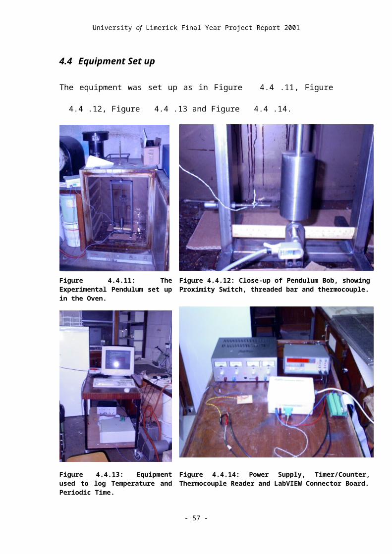
University of Limerick Final Year Project Report 2001
7.0 THE COMPENSATED PENDULUM
The compensated pendulum that has been analysed was designed and built by Dr.
Richard Stephen as part of his 30 day Vienna regulator. The clock is weight driven
and runs for 30 days between windings. As a result, it was designed
with the reduction of drivetrain friction as the top priority.
In order to allow the clock to remain accurate for the 30 days for
which it runs between windings, the pendulum is temperature
compensated, which means that it is designed to beat out the same
periodic time regardless of the expansion of its parts due to
temperature. The purpose of this project is to gauge the
effectiveness of this compensation.
Figure 6.1.22: The Compensated Pendulum
The compensation in the pendulum was designed to keep the centre of gravity of the
pendulum bob in the same place regardless of temperature. This allows the effective
length of the pendulum, that is, the distance from the pendulum pivot to the
pendulum's centre of gravity, denoted h in Section 2.8, to remain constant.
Compensation is achieved by making the pendulum rod from two different materials,
arranged in the correct ratio so that as one material expands due to the temperature,
the second material will expand in the opposite direction or contract in order to cancel
out the effect of the first one.
- 57 -

University of Limerick Final Year Project Report 2001
For the pendulum in question, the rod is made from steel and carbon fibre. The steel
expands due to temperature increases while the carbon fibre contracts to counteract
this expansion. In a pendulum where the bob is supported at its centre of gravity, the
ratio of the lengths of the two materials used to make up the pendulum should be in
inverse proportion to their coefficients of thermal expansion.
However, in the case of the pendulum being analysed, the pendulum bob is supported
at its base, causing the bob to expand upwards as the pendulum is heated. This
expansion was accounted for in the design calculations, but these calculations
assumed the bob to be symmetrical about a horizontal plane through its centre of
gravity, which is not the case in reality. This, as will be seen later is one of the reasons
the pendulum is not perfectly compensated.
The pendulum model which was analysed was modelled in three dimensions based on
a set of 2D drawings published in the British Horological Journal of August 2000.
Initially all the parts were drawn as separate ProEngineer files. These were then
imported into an assembly drawing to create the full assembly.
In order to confirm the interpretation of the drawings, image files displaying the
assembly from several angles were emailed to Dr. Richard Stephen, the pendulum's
designer. He was then able to confirm that the assembly was correct, as well as that
the material assigned to each part was correct.
- 58 -

University of Limerick Final Year Project Report 2001
7.1 The construction of the Compensated Pendulum
The full compensated pendulum assembly is made up of 15 separate parts. These are
named as in Table 4. Dimensioned Drawings of the Pendulum can be seen in
Appendix 9.10.
However, since neither the Mounting or the Split block oscillate with the pendulum,
these do not contribute to the overall mass of the pendulum. However, the Split block
does contribute to the periodic time since the oscillating length of the pendulum is
measured from the bottom edge of the split block, where the suspension spring
touches it, to the centre of gravity of the pendulum assembly. This relationship was
investigated using Finite Element Analysis in Section 7.3.
- 59 -

University of Limerick Final Year Project Report 2001
Table 4: Components of the Compensated Pendulum
No Component Description
1 Block Pin Holds Split Block in position in Mounting
2 Bob This is a weight hung from the pendulum rod. It gives the pendulum its characteristic behaviour along with the length of the rod
3 Bob Pin Prevents bob from turning on pendulum rod. Works in conjunction with Sleeve
4 CF Rod Carbon Fibre, Contracts as temperature rises to compensate pendulum
5 Clamp Clamps to Rod Top
6 Clamp Pin Locates suspension spring in clamp
7 Mounting Supports pendulum, connecting it to the rest of the clock
8 Rating Nut This supports the bob and allows the pendulum to be calibrated by winding the rating nut up and down
9 Rivet Holds suspension spring rigidly to Split Block
10 Rod Base Fits to the end of the Carbon Fibre Rod. Threaded for the rating nut and drilled to hold the Bob Pin
11 Rod Top Clamps the other end of the suspension spring
12 Screw Clamps the suspension spring between Rod Top and Clamp
13 Sleeve This is an interference fit into bob and engages with Bob Pin
14 Split Block Slit block to hold suspension spring
15 Spring Suspension Spring, flexes to allow pendulum to swing
See Appendix Sections 9.10 and 9.11 for dimensioned drawings of the pendulum
parts.
Table 5: Amalgamated Parts List
No Component Description
1 Base Assembly This is an amalgamation of the Bob Pin, Rating Nut and Rod Base.
2 Bob This is the same as the Bob in Table 4.
3 Carbon Fibre Rod This is the same as the Carbon Fibre rod in Table 4.
4 Sleeve This is the same as the Sleeve in Table 4.
5 Top Assembly Amalgamation of the clamp, clamp pin, Rod Top, screw and the part of the suspension spring which is not in the split block.
- 60 -
University of Limerick Final Year Project Report 2001
7.2 Analysis of the compensated pendulum using
ProEngineer and ProMechanica
In order to analyse the pendulum, unnecessary aesthetic features of the parts were
deleted. These features were not dimensioned in the drawings being worked from and
the removal of these features has a negligible effect on the overall mass properties of
the model, but makes its analysis less accurate as the dimensions of all these features
need to be known exactly if a completely exact result is required. The deleted features
are as follows;
All screw threads.
The fillets and ridges around the edges of the rating nut.
The groove in the screw that clamps the suspension spring into the top of the
pendulum rod.
The grooves cut into the reduced diameters at the ends of the steel parts of the
pendulum rod to glue the carbon fibre rod in position more securely.
See Appendix Section 9.10 and 9.11 for the details of the original assembly drawings
as compared to the drawings of the amalgamated parts.
Since no dimensions were given for the rating nut, the only requirement for the design
of this part was that it should be large enough to do its job and not heavy enough in
comparison to the bob that it has a significant effect on the calculated compensation.
The rating nut drawn was based on the photographs of the finished clock published by
the British Horological Institute.
- 61 -

University of Limerick Final Year Project Report 2001
To simplify the analysis, as well as increase the speed at which it can be performed,
parts which were connected rigidly together and made from the same material were
replaced by a single part, as the overall effect of a temperature change on a rigidly
connected set of parts of the same material is exactly the same as on a single solid part
the same shape.
In order to find the new dimensions for the pendulum, the formula
from Section 2.9 was used. The drawings of the amalgamated parts were copied and
the dimensions of the parts in the new files were changed to the dimensions calculated
for after a 25ºC temperature rise.
ProEngineer was then used to calculate the mass properties of the initial parts and
deformed parts. This information can be seen in Section 9.11 of the Appendix. The
new volume of the deformed part was also calculated in ProEngineer. Since the mass
of each part will remain constant, the change in density due to each part's expansion
was then calculated as in Table 7.
Once the new density was calculated for the deformed parts, it was put into the
ProEngineer model as a material property, thus allowing the mass properties for the
deformed part to be calculated correctly. The accuracy of the new density calculations
can be checked by comparing the mass derived by ProEngineer for each deformed
part with the mass of the original part calculated using the density at room
temperature.
- 62 -
University of Limerick Final Year Project Report 2001
The amalgamated parts were then assembled into the full pendulum, assembling the
initial and deformed parts in separate drawings and calculating the mass properties for
the initial and deformed pendulum assemblies using ProEngineer. These results can
be seen in Table 6 and Section 9.13.
7.3 Finite Element Analysis of the Split block and Suspension
Spring
Since the block pin, the rivet and the suspension spring are made of steel and the split
block is made from brass, a temperature change will cause stresses to build up
between these parts. Trying to predict this behaviour using manual calculations would
be extremely difficult, as the contact areas are curved, causing a variable stress
distribution where the pin and rivet interact with the block.
Figure 7.3.23: The Finite Element Analysis Model
- 63 -

University of Limerick Final Year Project Report 2001
Since the benchmark testing in Section 9.16 gave acceptable results, Finite Element
Analysis could then be confidently applied to the problem of the interaction of the
split block and the suspension spring.
A Finite Element Analysis model was built as shown in Figure 7.3.23, modelling the
suspension spring as a plate element, rigidly linked to the rivet and block pin, which
are modelled in 3D, with the split block modelled as a solid block with holes for the
pin and rivet, but no slit for the suspension spring, as it was not necessary due to the
spring being modelled as a 2D part, with its thickness set as a property.
The model was constrained as shown in the diagram in Figure 7.3.23, with the spring
corners constrained to only allow expansion in the XY plane, and the surfaces of the
block prevented from turning.
Contact areas were set up between the curved surfaces of the pin and rivet, and the
surfaces of the holes made for them in the block. A contact area, basically, is where
ProMechanica makes elements which link surfaces which are in contact, in order to
model how they interact as the model is loaded. Without the contact areas set up, the
volumes would pass through eachother without interacting.
Note also that the rivet protrudes beyond the surface of the split block. The reason for
this is that ProMechanica will automatically assume any curves or points which
coincide to be rigidly linked. This means that contact analysis could not be used for
the model as the rivet and block would already be linked rigidly.
- 64 -

University of Limerick Final Year Project Report 2001
In order to make the cross sectional area of the split block the same as for the actual
part, the thickness of the block was reduced by 0.1mm, as this is the thickness of the
slot which was cut into the block in the actual pendulum.
A measure was set for the Y displacement of a point on the bottom corner of the
block, relative to the co-ordinate system at the bottom corner of the spring. A
temperature change will cause the split block to move over the suspension spring,
reducing the free length of the suspension spring, but the expansion of the suspension
spring will act against this, to lengthen the pendulum. This is shown in Figure 7.4.25.
7.4 Results
The results shown in Figure 7.4.24 and Figure 7.4.25 indicate that the Finite Element
Analysis model is deforming as expected. It was known that the brass block would
expand relative to the other parts as it has a higher coefficient of expansion than the
steel parts, causing the diameters of the holes in the block to increase relative to the
diameters of the pin and rivet.
The suspension spring is pulling the pin and rivet together, causing spaces to open up
at the top of the hole for the pin and at the bottom of the rivet hole. The spaces shown
in Figure 7.4.24 and Figure 7.4.25 are greatly exaggerated due to the result being
scaled in order to make the change visible. The end of the split block was found to
displace by 1.8370089819655×10⁻³ mm relative to the bottom of the spring, indicating
a net increase in the length of the pendulum, though this increase would have been
2.75×10⁻³ mm if the edge of the block did not move relative to the suspension spring.
- 65 -
University of Limerick Final Year Project Report 2001
Figure 7.4.24: A plane cut through the deformed model, showing stress
Figure 7.4.25: A contour plot showing the displacements of the different parts of the model. The thin lines shown the displacement of the spring.
- 66 -

University of Limerick Final Year Project Report 2001
7.5 Results for Compensated Pendulum
Table 6: Mass Properties of the Compensated Pendulum Assembly before and after the Temperature Change as calculated by ProEngineer.
Original Deformed
Volume 98613.393 mm³ 98740.203 mm³
Surface Area 38407.444 mm² 38429.187 mm²
Average Density 7.86526E-09 Mg/mm³ 7.85516E-09 Mg/mm³
Mass 0.00077562 Mg 0.000775621 Mg
Centre of Gravity Distance -552.31794 mm -552.2966 mm
Inertia about top of Spring 240.44349 Mg·mm² 240.42605 Mg·mm²
Periodic Time 1.503166198 s 1.503139394 s
Change in Period: -26.80398096 µs
Pendulum Cumulative Error, Assuming Temperature Remains 25ºC Above
the Calibration Temperature
Maintained over a Day = -1.5406848 Sec/Day
Maintained over a Month = -46.2205 Sec/Month
These results show that the change in period for a temperature change of 25ºC is
about -27µs per period. This means that as the temperature rises, the clock will tend to
run faster rather than more slowly as is the case for the experimental pendulum. This
is due to the effect of the sleeve, the rating nut and the split block which are not
accounted for in the compensation calculations, as well as the extra length in the base
of the pendulum rod to allow the rating nut to be adjusted.
- 67 -

University of Limerick Final Year Project Report 2001
7.6 Sources of Error
7.6.1 Calculation Error
ProMechanica will output displacement values to 14 significant digits, though
rounding error contributes to the lower order decimal places as can be seen in the
benchmark analysis 9.18.1, 9.18.2 and 9.18.3.
ProEngineer will also take dimensional inputs to 14 significant digits, though it
usually rounds these to 6 places when displaying them. The calculation of the volume
by ProEngineer is given to 8 significant places, as is centre of gravity distance, which
may have some effect on the accuracy of the calculation. The density change
calculated using these volumes gives a figure that has less then 8 significant places, so
the error is more due to rounding in the volume calculation rather than in the density
calculation, which was performed using Microsoft Excel to 15 significant places.
Also, since the Carbon fibre rod is a composite, it cannot be assumed that its
coefficient of expansion is the same in all directions as was done for this analysis.
This will be a source of error, though, since the property of most interest is the
longitudinal expansion of the rod, and this was measured experimentally by Richard
Stephen [3], variations in the expansion of the rod in other directions will have far less
effect on the overall pendulum behaviour than the length change.
- 68 -

University of Limerick Final Year Project Report 2001
7.6.2 Experimental Error
The dimensions used for the experimental pendulum in the analysis of the
significance of the moment of inertia are as in the drawings. The actual values deviate
significantly from these, particularly the dimensions of the bob see dimensions used in
calculations in Section 9.3.1.
However, the change in periodic time is quite similar overall. The calculations shown
in Table 2 are for the measured dimensions of the bob, taken at approximately 21°C ±
1°C.
Circular error causes the pendulum's period to drop as the experiment progresses. This
is not really a problem as the pendulum half arc is held to under 2 degrees as
recommended in 3.1. In the graph showing the results, the trend of a decreasing period
as time passes can be seen Figure 5.3.19. The circular error effect gives the graphs a
logarithmic decrement, but does not prevent them from being compared to each other
overall.
The pendulum may have lost energy from its swing more quickly than it should have
due to the cardboard used to level the frame of the rig damping the pendulum
vibrations. Errors in one set of experiments performed by Robert Matthys were caused
by the roof beam he was hanging a pendulum from flexing[5]. Clocks using the same
length pendulum have also been noticed to interfere with eachother for the same
reason[3].
The pendulum is not compensated for pressure changes. This should not cause
significant problems as each set of experiments was run over one day and the duration
- 69 -

University of Limerick Final Year Project Report 2001
of each experiment was kept to approximately 15 minutes each time. This will totally
eliminate the significance of gravitational variation, though this is negligible even in
precision regulators[1].
The counter timer used to measure the period of the pendulum has no logging
capability. This means that it was necessary to manually type the 8 digit average of
each 10 periods, approximately every 7 seconds, while the computer logged the
temperature automatically every 5 seconds. This leaves potential for errors in the
transcription of readings from the counter timer to the computer during the
experiment, though the 7 seconds was more than enough to allow the period to be
typed and verified for each measurement.
Forwards and backwards vibration in the pendulum may affect the periodic time.
However, after the first two or three cycles there is no visible vibration in the
pendulum except for the periodic oscillation being measured. If the pendulum is
started carefully, even the initial vibrations can't be seen or felt by touching the frame
supporting the pendulum, so this source of error is unlikely to be significant.
Though the design of the experimental pendulum stated that it should be made
entirely from the same material, this does not eliminate the possibility that parts are
expanding at different rates. Since the thermal expansion coefficient is not usually
considered an important property, metal producers do not control it very tightly. This
means that there will almost certainly be variation from part to part in the test
pendulum. There can also be significant variations when the heat treatment is
changed[3]. The significance of this error cannot be quantified without measuring the
- 70 -

University of Limerick Final Year Project Report 2001
expansion coefficient for each part of the test pendulum and no facilities were
available to perform this task.
In order to start the pendulum, the door of the oven had to be opened each time. This
causes significant heat loss from the air around the pendulum and the pendulum itself,
but this was reduced by opening the door for as short a time as possible (Under 5
seconds), and leaving the oven turned on for a minute after the pendulum was started
so the temperature could stabilise again.
Another possible source of error is that the pendulum was not stood on a completely
level surface. This was virtually eliminated by the use of a spirit level to ensure that
the pendulum was hanging vertically before the experiment started. The pendulum
support frame was not moved during the course of the experiments, which means that
all readings taken will have the same error due to the rig being slightly off level.
From the variation in temperature results it is thought that the thermocouple amplifier
is the most likely a source of error in these measurements. More details of this are
given in Section 9.6.
There is also error due to the thermocouple measuring the air temperature around the
pendulum rather than the actual temperature of the pendulum. Ideally, thermocouples
should be fitted to holes in several parts of the pendulum, allowing the temperature
gradients throughout the pendulum to be measured. If the thermocouple was fitted to
the pendulum, however, the spring stiffness and hysteresis in the wiring connecting it
- 71 -

University of Limerick Final Year Project Report 2001
to the thermocouple reader will cause the pendulum to lose more energy with each
swing than it is losing due to air resistance, reducing the possible duration of each test.
Error due to air currents around the pendulum was kept to a minimum as the oven,
which is fan assisted, will be switched off while readings are being taken. Because the
temperature is being logged, the temperature variation in the oven will be known as
the experiment progresses, allowing compensated readings to be generated if the
temperature drop is significant. However, the experiment does make the assumption
that the air currents in the oven die down completely after the oven is turned off. The
actual results in Section 5.0, indicate that this was most certainly not the case.
Also, in a British Horological Journal article[5], an investigation was done into the
effects of changing the size of the clock case on the timekeeping of a pendulum. The
results of this indicated that, first of all, a pendulum of the size used in the practical
experimentation for this report was more susceptible to air currents than a larger
pendulum or a spherical bob, as the mass to surface area ratio for the small pendulum
is lower, therefore it will be affected more by the air surrounding it.
In the experiments described in the British Horological Journal, the nearer the walls of
the case were to the pendulum, the more they affected it, due to the pendulum itself
producing air currents as it oscillated. In the case of the experiments performed in this
project, however, the air currents were already present while the high temperature
readings were being taken.
- 72 -
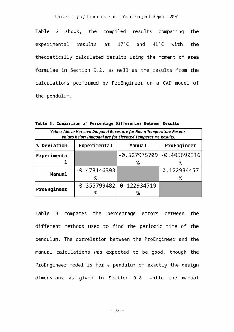
University of Limerick Final Year Project Report 2001
8.0 REFERENCES
[1] Burgess, Martin: ‘The Scandalous Neglect of Harrison’s Regulator Science’
(From ‘The Quest for Longitude: The Proceeding of the Longitude Symposium,
Harvard University, Cambridge Massachusetts, November 4-6 1993, p255-278).
[2] Holman, J.P.: Experimental Methods For Engineers, 5th Ed. 1989. p.299 to 313.
[3] http://www.bhi.co.uk (The British Horological Institute Website)
[4] National Instruments: LabVIEW user Manual and http://www.ni.com, the
National Instruments Website LabVIEW help pages.
[5] Matthys, Robert: The Clock Case and the Pendulum, British Horological Journal
August 1999, p263-266
[6] Meriam, J.L. and Kraige, L.G., Engineering Mechanics Volume 1, Statics 1993,
p241-245,
[7] Meriam, J.L. and Kraige, L.G., Engineering Mechanics Volume 2, Dynamics
1993, p594-597, p707, p657-661
[8] Murphy O.: Fundamental Applied Maths, Folens 1986, p301-334
[9] Roark and Young 5th Edition, Material Properties.
[10] Stephen, Richard: ‘A 30-day Vienna Regulator, 1’ British Horological Journal
March 2000 p100-102.
[11] Stephen, Richard: ‘A 30-day Vienna Regulator, 6’ British Horological Journal,
August 2000 p271-273.
- 73 -
University of Limerick Final Year Project Report 2001
8.1 Recommendations for Further Work
If further experiments are to be performed on the test pendulum, then some system to
screen it from outside air currents must be built. Building an enclosure for the
pendulum which has its own heating system would allow this error to be removed.
A levelling system using threaded bars or bolts put through the legs of the pendulum
rig frame would give more accurate levelling control, as well as less vibration
damping than the cardboard used for the previous experiments.
Fitting an escapement mechanism to the pendulum would allow it to be tested over a
longer time period. The escapement should be weight driven, as this is the most likely
arrangement to give a constant driving force to the escape wheel, as well as being
easier to implement than a spring arrangement, which would probably need a
remontoire See Section 9.1.
Converting the pendulum to use a suspension spring is not recommended, unless an
escapement is driving the pendulum and it is shielded from outside air currents
already. An arrangement such as this, with circular cheeks fitted to the suspension
spring, would allow the use of circular error to compensate for variations in arc angle
to be investigated.
Designing a system to allow the pendulum to be started remotely would make the
experiments more accurate, as the oven would not have to be opened in order to start
the pendulum. However, this is not worth doing until error due to the air currents in
- 74 -
University of Limerick Final Year Project Report 2001
the oven has been eliminated, or an alternative means of heating the pendulum has
been found.
The pendulum can be redesigned to have a variable mass moment of inertia. This can
be done through the use of interchangeable bobs of the same size made from different
materials. Another, more interesting option would be to use a bob whose mass
moment of inertia can be changed by making it from a stack of washers of different
materials, which slide onto the pendulum rod, the order of which can be changed to
maintain the same centre of gravity, but change the mass moment of inertia.
This would allow mass moment of inertia changes to be investigated separately to the
temperature effects, as the movement of the bob’s centre of gravity would be the same
regardless of the order the washers were fitted in, once the temperature change is the
same. This would allow the same equipment to be used to examine both mass moment
of inertia changes and temperature changes.
- 75 -

University of Limerick Final Year Project Report 2001
9.0 APPENDICES
- 76 -

University of Limerick Final Year Project Report 2001
9.1 Pendulum Nomenclature
Figure 9.1.26: Clock and Pendulum Nomenclature
- 77 -

University of Limerick Final Year Project Report 2001
Anchor: This is the anchor shaped plate the pallets are connected to.
Back Cock: This is the part of the clock which the pendulum mounts onto. The
Mounting part of the compensated pendulum serves this function.
Collet: This is the flange on the pallet arbor that the Pallets are connected to.
Crutch: This connects the pendulum to the escapement mechanism.
Crutch Pin: This connects the crutch to the pendulum rod.
Discharge Corner: This is the tip of the entrance or exit pallet tooth.
Entrance Pallet: This is the first tooth on the anchor. It engages with the escape wheel.
Escape Wheel: This is a gear wheel driven clockwise in the preceding diagram. The
turning of the escape wheel is regulated by the pallets gripping the teeth of the wheel.
Exit Pallet: This is the second tooth on the escapement mechanism which hooks into the
escape wheel. It is further around the escape wheel in the direction the escape wheel
travels than the Entrance Pallet
Face: This is the surface of the pallets, along which the teeth of the escape wheel slide as
the escapement operates.
Pallet Arbor: This is the shaft the Escapement Pallets are fitted to. The crutch is also
fitted to the pallet arbor.
Pendulum Bob: This is a weight hung from the end of the pendulum rod. It is usually
very heavy in comparison to the other oscillating parts of the pendulum, allowing the
distance from the pendulum pivot to the centre of gravity of the bob to be
approximated as the effective length h of the pendulum (See Section 2.8).
Pendulum Rod: This connects the spring and the bob together. It should be as rigid as
possible in order to prevent the pendulum assembly vibrating at higher frequencies
than the pendulum oscillation frequency, and in doing so affecting timekeeping.
Rating Nut: This screws up and down on the end of the pendulum rod and supports the
bob. Adjusting the rating nut changes the effective length of the pendulum, allowing
its periodic time to be adjusted.
Remontoire: This is a mechanism designed to deliver a constant torque to the escape
wheel to eliminate escapement variation. It works by storing energy from the weights
or springs used to drive the clock, and delivering it to the escape wheel in a controlled
manner.
Suspension Spring: This is a flat plate made from spring steel, which flexes to allow the
pendulum to oscillate.
- 78 -

University of Limerick Final Year Project Report 2001
9.2 Formulae used to Calculate the Mass Moment of Inertia
for Standard shapes.
For a Cuboid[7]:
Figure 9.2.27: Cuboid Mass Moment of Inertia
For a Cylinder[7]:
Figure 9.2.28: Cylinder Mass Moment of Inertia
- 79 -

University of Limerick Final Year Project Report 2001
9.3 Theoretical Calculations for the Test Pendulum
9.3.1 Calculations for the Test Pendulum using Actual Dimensions
(Figures in Bold Are the Driving Dimensions required to define the Shapes. Dimensions used were Measured from the Test Pendulum on 21/3/2001. The Temperature was 21 ± 1ºC)
Standard Temperature: 25 °C Temperature Rise Only accounting for length change instead
of MOI ChangeKnife Edge: Knife Edge:
Assumed solid Square Block. Assumed solid Square Block. Knife Edge:Diagonal 0.0306 m Diagonal 0.030608415 m 0.030608415 m
L 0.021637468 m L 0.021643418 m 0.021643418 mW 0.021637468 m W 0.021643418 m 0.021643418 mH 0.0601 m H 0.060116528 m 0.060116528 mIG 1.71892E-05 kgm² IG 1.71986E-05 kgm² 1.71892E-05 kgm²d -0.0153 m d -0.015304208 m -0.015304208 m
Volume 2.81376E-05 m³ Volume 2.81608E-05 m³ 2.81608E-05 m³Mass 0.220289411 kg Mass 0.220289411 kg 0.220289411 kg
IXX 6.87567E-05 kgm² IXX 6.87946E-05 kgm² 6.87851E-05 kgm²
Pendulum Rod: Pendulum Rod: Pendulum Rod:Assumed solid Cylinder. Assumed solid Cylinder.
L 0.6091 m L 0.609267503 m 0.609267503 mDiameter 0.01 m Diameter 0.01000275 m 0.01000275 m
DH 0.0199 m DH 0.019905473 m 0.019905473 mDT 0.0352 m DT 0.03520968 m 0.03520968 mIG 0.011581599 kgm² IG 0.011587969 kgm² 0.011581599 kgm²d 0.26935 m d 0.269424071 m 0.269424071 m
Volume 4.78386E-05 m³ Volume 4.78781E-05 m³ 4.78781E-05 m³Mass 0.374528416 kg Mass 0.374528416 kg 0.374528416 kg
IXX 0.038753419 kgm² IXX 0.038774736 kgm² 0.038768366 kgm²
Pendulum Bob: Pendulum Bob: Pendulum Bob:Assumed Cylinder with 10mm hole. Assumed Cylinder with 10mm hole.
L 0.1011 m L 0.101127803 m 0.101127803 mDiameter 0.05075 m Diameter 0.050763956 m 0.050763956 m
Volume 0.000204509 m³ Volume 0.000204678 m³ 0.000204678 m³Mass 1.60110356 kg Mass 1.60110356 kg 1.60110356 kg
IG 0.001621502 kgm² IG 0.001622394 kgm² 0.001621502 kgm²Hole L 0.1011 m Hole L 0.101127803 m 0.101127803 m
Hole Dia 0.01 m Hole Dia 0.01000275 m 0.01000275 mHole Vol -7.94038E-06 m³ Hole Vol -7.94693E-06 m³ -7.94693E-06 m³
Hole Mass -0.062165199 kg Hole Mass -0.062165199 kg -0.062165199 kgHole IG -5.33388E-05 kgm² Hole IG -5.33682E-05 kgm² -5.33388E-05 kgm²
Total Vol 0.000196569 m³ Total Vol 0.000196731 m³ 0.000196731 m³Total Mass 1.538938361 kg Total Mass 1.538938361 kg 1.538938361 kg
Total IG 0.001568163 kgm² Total IG 0.001569026 kgm² 0.001568163 kgm²d 0.5006 m d 0.500737665 m 0.500737665 m
IXX 0.38722667 kgm² IXX 0.387439674 kgm² 0.387438812 kgm²
- 80 -
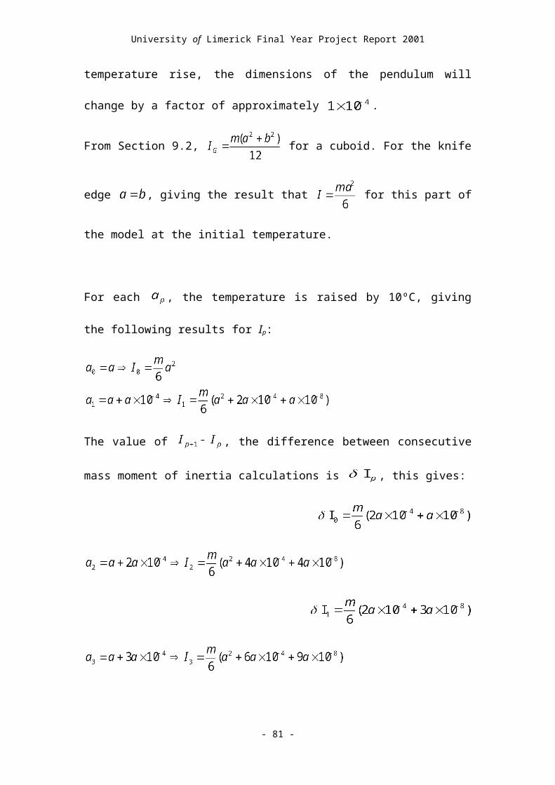
University of Limerick Final Year Project Report 2001
Overall Totals: Overall Totals: Overall Totals:Volume 0.000272545 m³ Volume 0.00027277 m³ 0.00027277 m³
Mass 2.133756188 kg Mass 2.133756188 kg 2.133756188 kgIXX 0.426048846 kgm² IXX 0.426283205 kgm² 0.426275962 kgm²
Periodic Time Calculation: Periodic Time Calculation: Periodic Time Calculation:LEQ 0.406748132 m LEQ 0.406859988 m 0.406859988 m
1.405769274 s 1.405962554 s 1.40595061 sChange in 0.00019328 s 0.000181336 s -6.179710186 %
9.3.2 Calculations for the Test Pendulum using Theoretical Dimensions
(Figures in Bold Are the Driving Dimensions required to define the Shapes)Standard Temperature: 25 °C Temperature Rise Not accounting for
changes in Knife Edge: Knife Edge: Moment of InertiaAssumed solid Square Block. Assumed solid Square Block. Knife Edge:
Diagonal 0.03 m Diagonal 0.03000825 m 0.03000825 mL 0.021213203 m L 0.021219037 m 0.021219037 m
W 0.021213203 m W 0.021219037 m 0.021219037 mH 0.06 m H 0.0600165 m 0.0600165 mIG 1.58537E-08 Mgm² IG 1.58624E-08 Mgm² 1.58537E-08 Mgm²d -0.015 m d -0.015004125 m -0.015004125 m
Volume 2.70000E-05 m³ Volume 2.70223E-05 m³ 2.70223E-05 m³Mass 0.000211383 Mg Mass 0.000211383 Mg 0.000211383 Mg
IXX 6.34149E-08 Mgm² IXX 6.34498E-08 Mgm² 6.34411E-08 Mgm²
Pendulum Rod: Pendulum Rod: Pendulum Rod:Assumed solid Cylinder. Assumed solid Cylinder.
L 0.61 m L 0.61016775 m 0.61016775 mDiameter 0.01 m Diameter 0.01000275 m 0.01000275 m
DH 0.02 m DH 0.0200055 m 0.0200055 mPin Dia 0.005 m Pin Dia 0.005001375 m 0.005001375 m
IG 1.1633E-05 Mgm² IG 1.16394E-05 Mgm² 1.1633E-05 Mgm²d 0.27 m d 0.27007425 m 0.27007425 m
Volume 4.79093E-05 m³ Volume 4.79488E-05 m³ 4.79488E-05 m³Mass 0.000375082 Mg Mass 0.000375082 Mg 0.000375082 Mg
IXX 3.89765E-05 Mgm² IXX 3.89979E-05 Mgm² 3.89915E-05 Mgm²
- 81 -

University of Limerick Final Year Project Report 2001
Pendulum Bob: Pendulum Bob: Pendulum Bob:Assumed Cylinder with 10mm hole. Assumed Cylinder with 10mm hole.
L 0.1 m L 0.1000275 m 0.1000275 mDiameter 0.05 m Diameter 0.05001375 m 0.05001375 m
Volume 0.00019635 m³ Volume 0.000196512 m³ 0.000196512 m³Mass 0.001537221 Mg Mass 1.537E-03 Mg 1.537E-03 Mg
IG 1.52121E-06 Mgm² IG 1.52204E-06 Mgm² 1.52121E-06 Mgm²Hole L 0.1 m Hole L 0.1000275 m 0.1000275 m
Hole Dia 0.01 m Hole Dia 0.01000275 m 0.01000275 mHole Vol -7.85398E-06 m³ Hole Vol -7.86046E-06 m -7.86046E-06 m
Hole Mass -6.149E-05 Mg Hole Mass -6.149E-05 Mg -6.149E-05 MgHole IG -5.1625E-08 Mgm² Hole IG -5.16534E-08 Mgm² -5.1625E-08 Mgm²
Total Vol 0.000188496 m³ Total Vol 0.000188651 m³ 0.000188651 m³Total Mass 0.001475732 Mg Total Mass 0.001475732 Mg 0.001475732 Mg
Total IG 1.46958E-06 Mgm² Total IG 1.47039E-06 Mgm² 1.46958E-06 Mgm²d 0.5025 m d 0.502638188 m 0.502638188 m
IXX 0.000374101 Mgm² IXX 0.000374307 Mgm² 0.000374306 Mgm²
Overall Totals: Overall Totals: Overall Totals:Volume 0.000263405 m³ Volume 0.000263622 m³ 0.000263622 m³
Mass 0.002062197 Mg Mass 0.002062197 Mg 0.002062197 MgIXX 4.13140954254399E-04 Mgm² IXX 4.13368213023024E-04 Mgm² 4.13360996887402E-04
Mgm²
Periodic Time Calculation: Periodic Time Calculation: Periodic Time Calculation:LEQ 0.407166107 m LEQ 0.407278078 m 0.407278078 m
1.407400876 s 1.40759438 s 1.407582094 sChange in 0.000193504 s 0.000181218 s -6.349307679
Half Period: 0.703700438 s 0.70379719 s 0.703791047 s
- 82 -

University of Limerick Final Year Project Report 2001
9.4 Calibration of the K Type Thermocouple Amplifier
When two dissimilar metals are brought into contact with each other, an e.m.f. or
voltage is induced between them. This is known as the Seebeck effect. If there is
temperature gradient along either of both metals, the e.m.f. (Electro-Motive Force)
will change slightly. This is called the Thomson effect[2].
The e.m.f.’s developed by the thermocouple are extremely small and must be
amplified before they can be measured by
systems such as LabVIEW. This is done by
the use of a thermocouple amplifier as shown
in Figure 9.4.29.
Figure 9.4.29: Thermocouple Amplifier
In order to calibrate the amplifier, an adjustment screw (See red arrow in Figure
9.4.29) is used to change the gain of the circuit, thereby adjusting the amount by
which the output voltage changes for a given temperature change.
The Thermocouple used for this experiment is a ‘K’ Type thermocouple, which means
that it uses a Chromel Alumel junction to produce its e.m.f.. The e.m.f. at 10°C is
approximately 0.412 millivolts[2].
In order to zero the voltage output from the thermocouple amplifier, a microchip
designed for thermocouple amplifiers is used. This has a cold junction, which
automatically fixes the zero on the thermocouple at 0ºC.
- 83 -
University of Limerick Final Year Project Report 2001
The thermocouple was calibrated using a second thermocouple that had previously
been professionally calibrated. The reference temperatures used for the calibration
were water at 80°C and room temperature at 20°C. Skin temperature at 31°C was used
as a test to confirm that the calibration was correct. All readings agreed to within
±0.5º, which was adequate for the experimental requirements.
It should be noted that ‘K’ Type thermocouples are considered ‘satisfactory, but not
recommended’ for use at temperatures below 315°C[2], however, the ± 1ºC accuracy
recorded from the calibration procedure was considered adequate.
9.5 LabVIEW
LabVIEW is a program written by the National Instruments Company. It is designed
to be used for experimental and practical data gathering and processing, as well as for
controlling other equipment through its analogue and digital outputs.
LabVIEW stands for Laboratory Virtual Instrument Engineering Workshop and was
written in ‘G’, a 32 bit graphical programming language. LabVIEW programs have
two parts, the front panel and the block diagram[4].
For the experimental work required for this project, LabVIEW was intended to be
used to log both the pendulum periodic time from the proximity switch, as well as the
temperature from the thermocouple fitted to the pendulum rig frame as in Section 4.4,
completely automating the data gathering process for the experimental work.
- 84 -

University of Limerick Final Year Project Report 2001
LabVIEW is a relatively user friendly program, as it is programmed graphically. The
resulting programs look much like a circuit diagrams, which makes it easier to find
faults and to write the programs in the first place.
The LabVIEW interface is split into two basic parts. The first is the control window.
This displays the results measured by LabVIEW, as well as allowing the person using
the program to change the program settings. The second window is the diagram
window. This displays the program as an electrical type schematic.
However, because of the user friendly interface, there is a lot of processor overhead,
which affects the results measured by LabVIEW for precision timing applications.
This caused considerable trouble as before the program was written, the National
Instruments technical support was consulted, and they said that the program was
capable of taking measurements to the accuracy required, since they assumed the
computer being used was not a limiting factor.
Three weeks were spent, between learning to use LabVIEW and actually writing the
program to log the periodic times, only to discover in testing a prototype program that
the readings being taken were inconsistent.
The speed at which the program runs could be improved by using a faster computer,
but the Pentium 133MHz which was allocated for the job should really have been
more than adequate. The program, which was supposed to log all the periodic times
while the experiment was in progress was never finished, as the initial testing done on
- 85 -
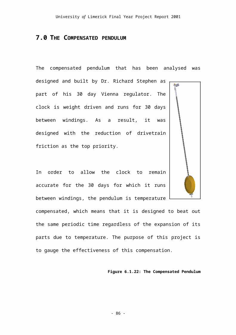
University of Limerick Final Year Project Report 2001
a non-logging version of the program showed errors in the time readings as described
in Section 9.7.
However, LabVIEW was still used to log the temperature readings from the
thermocouple, as this was not a timing intensive operation, so a second program was
written to do this. This program did exactly what was required of it, and the diagram
for this program can be seen in Figure 9.6.30.
9.5.1 Understanding LabVIEW diagrams
LabVIEW diagrams are laid out much like a circuit in that each block on the diagram
performs some sort of operation on the circuit. This is determined by the inputs wired
in to the block and the type of block chosen. The program block performs its function
and outputs the result through more wires connected to its outputs.
Multiple blocks can be wired in parallel if necessary, making LabVIEW more flexible
than most languages in the way it can be programmed, as most languages require
linear command sequences.
Wires connecting blocks are colour coded to allow them to be identified quickly. The
type of data carried by the wire determines its colour as follows;
Blue - Integer Number
Orange - Double Precision Number
Pink - Text String
Green - Boolean True/False
- 86 -
University of Limerick Final Year Project Report 2001
Thick blue or orange - Multiple values of integer or double precision number
types
Inputs can either be set by using constants in the diagram, which show up as thick
bordered boxes with numbers in them, or else by taking values from the control
window. This method allows the user to change values as they require without having
to look at the block diagram each time.
Inputs from the control window are displayed as thick bordered boxes with an
abbreviation for the number type in them such as DBL for double precision, I16 or
I32 for 16 or 32 bit integers and V16 or V32 for 16 or 32 bit positive integers. The
outputs from the program are boxes with thin borders, which use the same numerical
notation as the inputs. The values contained in these blocks are displayed in the
control window.
Blocks with yellow backgrounds are used to denote mathematical or Boolean
functions. They use as 'or' and as 'and', with the rest of the symbols being familiar
to most people. Blocks with yellow backgrounds and blue text are used to control the
for and while loop functions.
For loops repeat the contents of the loop as many times as the value wired to the N
box in the loop and while loops continuously repeat the contents of the loop until a
certain condition changes from true to false. In the for loop i is the number of
iterations the loop has performed at any given time. The circular arrow in the while
loop is wired to a Boolean variable and controls when the loop stops and stops.
- 87 -

University of Limerick Final Year Project Report 2001
9.6 The temperature Logging Program
The temperature log diagram uses a for loop with a delay which can be adjusted by
changing the value of the ‘Time Interval between readings’ variable, the make the
loop execute at given intervals. Note that the change in the thickness of the wires
outputting from the for loop indicate that the wires carry multiple values.
These values are written to a text file as the logged temperature readings, as well as to
an XY Graph, which displays the data gathered in the control window after the
program has finished running. The values recorded by the temperature logging
program can be seen in Section 9.20 and 9.21.
Figure 9.6.30: Temperature Logging Program Block Diagram
- 88 -

University of Limerick Final Year Project Report 2001
Figure 9.6.31: Control Window for Temperature Logging Program
9.7 The Periodic Time Logging Program
This program was written to measure the periodic time of the pendulum for each
period occurring during the experiment. It does this by measuring the width of the
high pulse from the proximity switch and adding it to the width of the low pulse, also
measured by LabVIEW through a different channel.
It was necessary to do this as LabVIEW can only be made to measure high pulses, so
the signal from which the low pulse was measured had to be inverted, using a 7404
Inverter chip. This is a not gate and converts the high pulses to low pulses and vice
versa. The wiring diagram for this arrangement is shown in the control window in
Figure 9.7.32.
- 89 -

University of Limerick Final Year Project Report 2001
Figure 9.7.32: Control Window for the Periodic Time Logging Program
Figure 9.7.33: Block Diagram for the Periodic Time Logging Program
The pulses are measured using a system of counters, driven from a 2MHz clock built
into the LabVIEW board. Figure 9.7.33 shows the block diagram of this program.
This was thought to be accurate enough for the purposes of the experiment, though
there were a few limiting factors, namely that the maximum counter size which
- 90 -
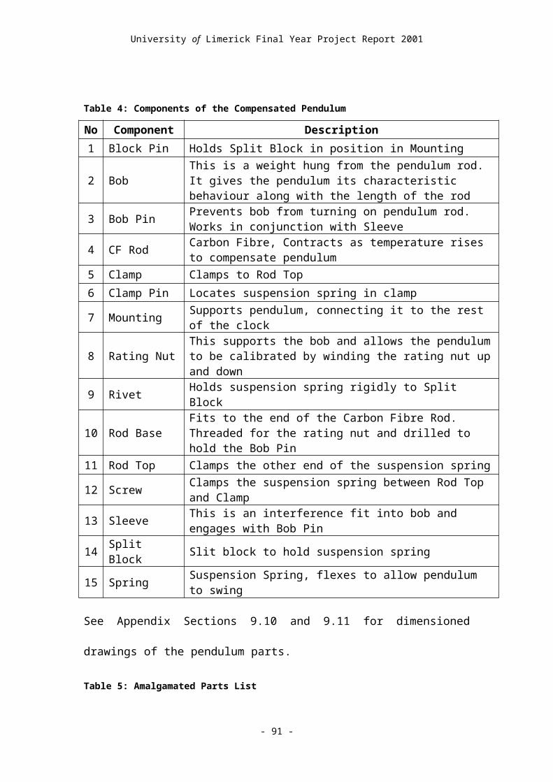
University of Limerick Final Year Project Report 2001
LabVIEW can handle is 65,535, which means that the length of each period measured
has to be less than 65,535 times the minimum time unit. Because of this, a sample rate
of 90,000 Hz was chosen, allowing a maximum pulse width of 0.727 Seconds to be
measured, as this will give the best time resolution, without causing the counters to
overflow.
However, when the program was tested, it was discovered that when the same signal
was sent into both pulse measuring loops, the values read from the program for Count
and Count 2 disagreed by 1 every third period or so, showing an error in the values
measured by the computer. This error is due to the computer taking too long to run the
program, as, though the two loops are wired in parallel, the computer must execute
them one after another, causing the reading from the second loop to be larger than the
reading from the first.
There is also the possibility that there is a delay caused by the computer running the
program too slowly before it even takes the first reading, leading to more error. Also,
when the 7404 chip is fitted into the circuit, it may also add a small delay to the
signal.
If the program was to be modified to write the periodic times to a separate text file,
the two pulse length measuring loops would have to be placed in another loop, which
would make the computer take even longer to run the program, increasing error
further. The temperature logging program will also add to the error for the same
reason, as it would also be running while the periodic time measuring program is
running, and therefore take up computer processing time.
- 91 -
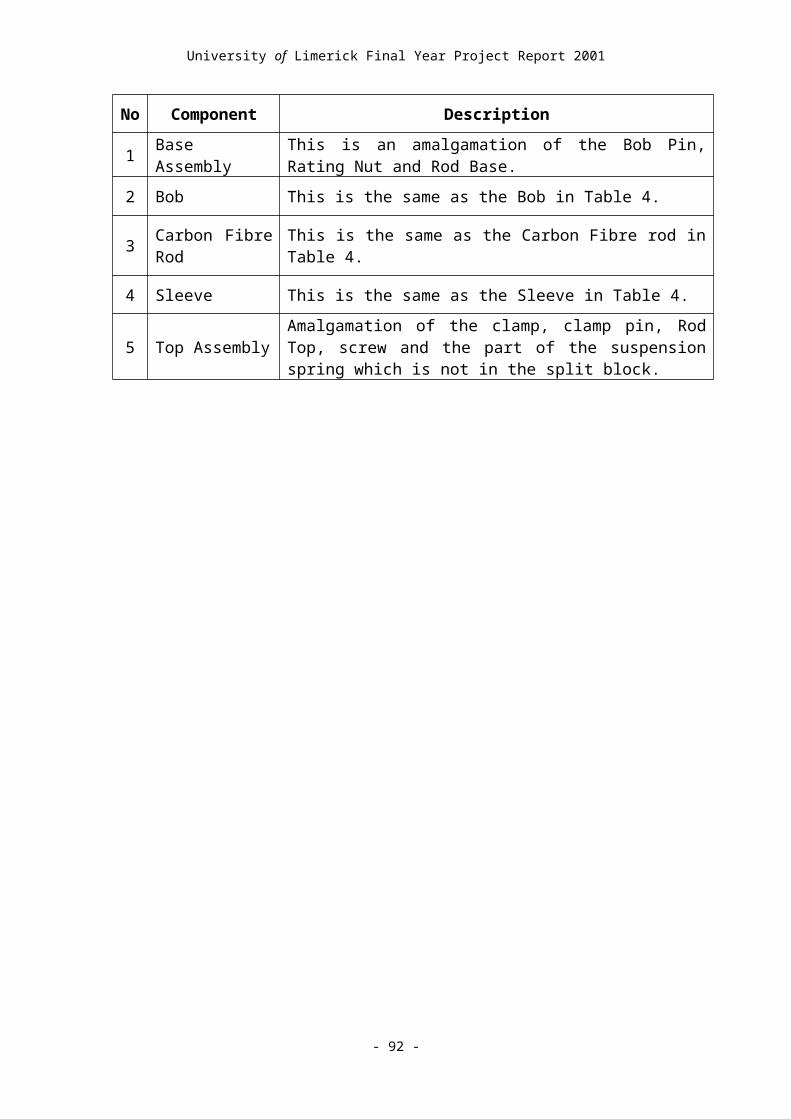
University of Limerick Final Year Project Report 2001
It was concluded from this that, though it is possible for LabVIEW to perform the
periodic time logging function, no confidence can be expressed as to its accuracy. It is
for this reason that the timer counter was used instead of LabVIEW for periodic time
measurement, as this was designed for the sole purpose of taking these measurements.
However, LabVIEW was used for recording the temperature read by the
thermocouple at regular time intervals, as this does not require precision timing and
saves a considerable amount of work.
- 92 -
University of Limerick Final Year Project Report 2001
9.8 Construction Drawings of the Test Pendulum
The actual Dimensions of the test pendulum which was built can be found in the
theoretical calculations Section 9.3.1, which uses the design dimensions and 9.3.2,
which uses the actual dimensions.
- 93 -

University of Limerick Final Year Project Report 2001
Figure 9.8.34:Test Pendulum Assembly
Figure 9.8.35: Close up of Ruler, proximity switch, threaded bar and Bob
- 94 -

University of Limerick Final Year Project Report 2001
PENDULUM ASSEMBLY DRAWINGS First Angle Projection All Dimensions in Millimetres
Part Name: Pendulum Bob Material: Steel Design by Cormac Eason 9731318 15/11/2000
- 95 -

University of Limerick Final Year Project Report 2001
PENDULUM ASSEMBLY DRAWINGS First Angle Projection All Dimensions in Millimetres
Part Name: Knife Edge Material: Steel Design by Cormac Eason 9731318 15/11/2000
- 96 -
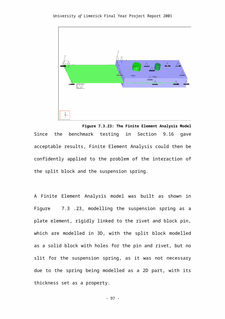
University of Limerick Final Year Project Report 2001
PENDULUM ASSEMBLY DRAWINGS First Angle Projection All Dimensions in Millimetres
Part Name: Pendulum Mounting Material: Steel Design by Cormac Eason 9731318 15/11/2000
- 97 -
University of Limerick Final Year Project Report 2001
PENDULUM ASSEMBLY DRAWINGS First Angle Projection All Dimensions in Millimetres
Part Name: Pin (2 off) Material: Steel Design by Cormac Eason 9731318 15/11/2000
- 98 -

University of Limerick Final Year Project Report 2001
PENDULUM ASSEMBLY DRAWINGS First Angle Projection All Dimensions in Millimetres
Part Name: Pendulum Rod Material: Steel Design by Cormac Eason 9731318 15/11/2000
- 99 -

University of Limerick Final Year Project Report 2001
PENDULUM ASSEMBLY DRAWINGS First Angle Projection All Dimensions in Millimetres
Part Name: Proximity Switch Mounting Material: Steel Design by Cormac Eason 9731318 15/11/2000
- 100 -

University of Limerick Final Year Project Report 2001
9.9 Details of the Compensated Pendulum
9.9.1 The Parts of the Compensated Pendulum
Component Material Description
Block Pin Steel Holds Split Block in position in Mounting
Bob Brass This is weight hung from the rod gives the pendulum its behaviour
Bob Pin Steel Prevents bob from turning on pendulum rod. Works in conjunction with Sleeve
Carbon Fibre Rod
Carbon Fibre
Contracts as temperature rises to compensate pendulum
Clamp Steel Clamps to Rod Top
Clamp Pin Steel Locates suspension spring in clamp
Mounting Steel Supports pendulum, connecting it to the rest of the clock
Rating Nut Steel This supports the bob and allows the pendulum to be calibrated by winding the rating nut up and down
Rivet Steel Holds suspension spring rigidly to Split Block
Rod Base Steel Fits to the end of the Carbon Fibre Rod. Threaded for the rating nut and drilled to hold the Bob Pin
Rod Top Steel Clamps the other end of the suspension spring
Screw Steel Clamps the suspension spring between Rod Top and Clamp
Sleeve Steel This is an interference fit into bob and engages with Bob Pin
Split Block Brass Slit block to hold suspension spring
Spring Steel Suspension Spring, flexes to allow pendulum to swing
- 101 -

University of Limerick Final Year Project Report 2001
9.9.2 The Amalgamated Parts which were Analysed
Component Material Description
Base Assembly Steel This is an amalgamation of the Bob Pin, Rating Nut and Rod Base.
Bob Brass This is the same as the Bob in the preceding Table.
Carbon Fibre Rod Carbon Fibre
This is the same as the Carbon Fibre rod in the preceding Table.
Sleeve Steel This is the same as the Sleeve in the preceding Table.
Top Assembly SteelAmalgamation of the part of the clamp, clamp pin, Rod Top, screw and the part of the suspension spring which is not in the split block.
9.10Dimensioned Drawings of Compensated Pendulum Parts
All Dimensions are in millimetres.
Figure 9.10.36: Block Pin and Clamp Pin are both exactly the same
- 102 -

University of Limerick Final Year Project Report 2001
Figure 9.10.37: Pendulum Bob
Figure 9.10.38: Bob Pin
- 103 -

University of Limerick Final Year Project Report 2001
Figure 9.10.39: Carbon Fibre Rod
Figure 9.10.40: Clamp
- 104 -
University of Limerick Final Year Project Report 2001
Figure 9.10.41: Mounting
Figure 9.10.42: Rating Nut
- 105 -
University of Limerick Final Year Project Report 2001
Figure 9.10.43: Rivet
Figure 9.10.44: Rod Base
- 106 -

University of Limerick Final Year Project Report 2001
Figure 9.10.45: Screw
Figure 9.10.46: Suspension Spring
- 107 -

University of Limerick Final Year Project Report 2001
Figure 9.10.47: Rod Top
Figure 9.10.48: Sleeve
Figure 9.10.49: Split Block
- 108 -
University of Limerick Final Year Project Report 2001
9.11Amalgamated Parts Analysed
Figure 9.11.50: Base Assembly
Figure 9.11.51: Deformed Base Assembly
- 109 -

University of Limerick Final Year Project Report 2001
Figure 9.11.52: Deformed Pendulum Bob
Figure 9.11.53: Deformed Carbon Fibre Rod
- 110 -

University of Limerick Final Year Project Report 2001
Figure 9.11.54: Deformed Sleeve
Figure 9.11.55: Assembly of Bottom of Pendulum, showing bob, bob pin, rating nut, rod base, carbon fibre rod and sleeve.
- 111 -

University of Limerick Final Year Project Report 2001
Figure 9.11.56: Top Assembly
Figure 9.11.57: Deformed Top Assembly
Figure 9.11.58: Top of Pendulum assembly, showing mounting, split block, block pin, rivet, suspension spring, clamp, screw, clamp pin, top rod and carbon fibre rod.
- 112 -

9.12Comparison of Separate Parts of Compensated Pendulum with Combined Parts
Table 7: Density changes in the parts of the Compensated Pendulum before and after the 25ºC Temperature rise.
Part Initial Volume Deformed Volume Material New Density
Bob 85216.099 mm³ 85337.589 mm³ Brass 8.39703E-09 Mg /mm³
Carbon Fibre Rod 6122.3358 mm³ 6121.9684 mm³ Carbon Fibre 3.40095E-10 Mg /mm³
Rod Base 2640.0525 mm³ 2641.915 mm³ Steel 7.82348E-09 Mg /mm³
Sleeve 3307.5628 mm³ 3310.2923 mm³ Steel 7.82254E-09 Mg /mm³
Rod Top 1327.3429 mm³ 1328.4377 mm³ Steel 7.82255E-09 Mg /mm³
9.13Compensated Pendulum Mass Properties as Calculated
by ProEngineer
9.13.1 Initial Pendulum Mass Properties with respect to Co-ordinate system at
top of suspension spring. Ixx is inertia about pendulum rotation axis.
VOLUME = 9.8613393e+04 MM^3
SURFACE AREA = 3.8407444e+04 MM^2
AVERAGE DENSITY = 7.8652590e-09 TONNE / MM^3
MASS = 7.7561988e-04 TONNE
CENTER OF GRAVITY with respect to ACS0 coordinate frame:
X Y Z 8.3895504e-03 -5.5231794e+02 0.0000000e+00 MM
INERTIA with respect to ACS0 coordinate frame: (TONNE * MM^2)
INERTIA TENSOR:
Ixx Ixy Ixz 2.4044349e+02 3.5058641e-03 0.0000000e+00
Iyx Iyy Iyz 3.5058641e-03 4.0771561e-01 0.0000000e+00
Izx Izy Izz 0.0000000e+00 0.0000000e+00 2.4005738e+02
INERTIA at CENTER OF GRAVITY with respect to ACS0 coordinate frame:
(TONNE * MM^2)
INERTIA TENSOR:
Ixx Ixy Ixz 3.8366886e+00 -8.8125062e-05 0.0000000e+00
Iyx Iyy Iyz -8.8125062e-05 4.0771556e-01 -5.8148438e-07
Izx Izy Izz 0.0000000e+00 -5.8148438e-07 3.4505778e+00
PRINCIPAL MOMENTS OF INERTIA: (TONNE * MM^2)
I1 I2 I3 4.0771556e-01 3.4505778e+00 3.8366886e+00
ROTATION MATRIX from ACS0 orientation to PRINCIPAL AXES:
0.00003 0.00000 1.00000
1.00000 0.00000 -0.00003
0.00000 1.00000 0.00000
ROTATION ANGLES from ACS0 orientation to PRINCIPAL AXES (degrees):
angles about x y z 0.000 89.999 90.000
RADII OF GYRATION with respect to PRINCIPAL AXES:
R1 R2 R3 2.2927367e+01 6.6699326e+01 7.0332137e+01 MM
---------------------------------------------
MASS PROPERTIES OF COMPONENTS OF THE ASSEMBLY
(in assembly units and the ACS0 coordinate frame)
DENSITY MASS C.G.: X Y Z
SPRINGBASE MATERIAL: STEEL
7.82900e-09 1.03918e-05 0.00000e+00 -3.31527e+01 0.00000e+00
CF_ROD MATERIAL: CARBON FIBRE
3.40075e-10 2.08205e-06 0.00000e+00 -3.05400e+02 0.00000e+00
PENDULUM_BASE MATERIAL: STEEL
7.82900e-09 2.06690e-05 -4.74147e-03 -5.96982e+02 0.00000e+00
BOB MATERIAL: BRASS
8.40900e-09 7.16582e-04 0.00000e+00 -5.59757e+02 0.00000e+00
SLEEVE MATERIAL: STEEL
7.82900e-09 2.58949e-05 2.55097e-01 -5.39000e+02 0.00000e+00
9.13.2 Deformed Pendulum Mass Properties with respect to Co-ordinate
system at top of suspension spring. IXX is inertia about pendulum
rotation axis.
VOLUME = 9.8740203e+04 MM^3
SURFACE AREA = 3.8429187e+04 MM^2
AVERAGE DENSITY = 7.8551717e-09 TONNE / MM^3
MASS = 7.7562125e-04 TONNE
CENTER OF GRAVITY with respect to ACS0 coordinate frame:
X Y Z 8.3918120e-03 -5.5229660e+02 0.0000000e+00 MM
INERTIA with respect to ACS0 coordinate frame: (TONNE * MM^2)
INERTIA TENSOR:
Ixx Ixy Ixz 2.4042605e+02 3.5066400e-03 0.0000000e+00
Iyx Iyy Iyz 3.5066400e-03 4.0810290e-01 0.0000000e+00
Izx Izy Izz 0.0000000e+00 0.0000000e+00 2.4003957e+02
INERTIA at CENTER OF GRAVITY with respect to ACS0 coordinate frame:
(TONNE * MM^2)
INERTIA TENSOR:
Ixx Ixy Ixz 3.8371102e+00 -8.8185465e-05 0.0000000e+00

Iyx Iyy Iyz -8.8185465e-05 4.0810284e-01 -5.8203632e-07
Izx Izy Izz 0.0000000e+00 -5.8203632e-07 3.4506324e+00
PRINCIPAL MOMENTS OF INERTIA: (TONNE * MM^2)
I1 I2 I3 4.0810284e-01 3.4506324e+00 3.8371102e+00
ROTATION MATRIX from ACS0 orientation to PRINCIPAL AXES:
0.00003 0.00000 1.00000
1.00000 0.00000 -0.00003
0.00000 1.00000 0.00000
ROTATION ANGLES from ACS0 orientation to PRINCIPAL AXES (degrees):
angles about x y z 0.000 89.999 90.000
RADII OF GYRATION with respect to PRINCIPAL AXES:
R1 R2 R3 2.2938233e+01 6.6699795e+01 7.0335938e+01 MM
---------------------------------------------
MASS PROPERTIES OF COMPONENTS OF THE ASSEMBLY
(in assembly units and the ACS0 coordinate frame)
DENSITY MASS C.G.: X Y Z
SPRINGBASE_DEFORMED MATERIAL: STEEL
7.82255e-09 1.03918e-05 0.00000e+00 -3.31609e+01 0.00000e+00
CF_ROD_DEFORMED MATERIAL: CARBON FIBRE
3.40099e-10 2.08208e-06 0.00000e+00 -3.05411e+02 0.00000e+00

PENDULUM_BASE_DEFORMED MATERIAL: STEEL
7.82395e-09 2.06702e-05 -4.74334e-03 -5.96989e+02 0.00000e+00
BOB_DEFORMED MATERIAL: BRASS
8.39703e-09 7.16582e-04 0.00000e+00 -5.59735e+02 0.00000e+00
SLEEVE_DEFORMED MATERIAL: STEEL
7.82254e-09 2.58949e-05 2.55167e-01 -5.38974e+02 0.00000e+00

9.14Carbon Fibre Rod Details
Precise details of the Carbon Fibre rod were not available, so the following
measurements were taken for a rod in the possession of Dr. Richard Stephen, thus
allowing the density of the Carbon Fibre to be calculated.
Length of rod 750 mm
OD of rod 4.90 mm
ID of rod 2.90 mm
Mass of rod 12.5 ± 0.5 grammes
Derived Density of Rod Material 3.40075E-10 Mg/mm³

9.15Properties of the Materials used
Steel: ProEngineer Units In SI Units
Density: 7.829E-09 tonnes/mm³ = 7829 kg/m³
Thermal Expansion Coefficient: 1.100E-05 mm/mm°C = 1.100E-05 m/m°C
Brass:
Density: 8.409E-09 tonnes/mm³ = 8409 kg/m³
Thermal Expansion Coefficient: 1.900E-05 mm/mm°C = 1.900E-05 m/m°C
Carbon Fibre:
Density: 3.40075E-10 tonnes/mm³ = 340.0746647 kg/m³
Thermal Expansion Coefficient: -8.000E-07 mm/mm°C = -8.000E-07 m/m°C
Acceleration due to Gravity: g 9806.65 mm/s² = 9.80665 m/s²Material Densities are from Roark and Young 5th Edition[9] as used by ProMechanica
Library. Material coefficients of expansion are from Richard Stephen’s Article in the
British Horological Journal[11].

9.16Benchmarking
In order to be confident that the Finite Element Analysis was giving the correct
results, it was necessary to perform some basic analyses on parts of known geometry
for which the deformation after a temperature increase is known.
The shape chosen was a cylinder 1000 mm high with a diameter of 1000 mm. The
deformed shape of this cylinder after a 25ºC temperature rise was then calculated
theoretically for the three materials being used, using the expansion equation in
Section 2.9.
The model was meshed and constrained as shown in Figure 9.16.59. The constraints
prevent the point at the origin of the co-ordinate system from moving in any direction,
while the point opposite it along the x-axis is free to move in the x direction. The
point opposite the origin in the y direction is free to move in y, while the point on the
opposite diagonal is free in both x and y, but constrained in z. These constraints hold
the xy-plane through the
centre of the cylinder
vertical, while not affecting
the overall expansion of the
cylinder.
Figure 9.16.59: The Finite Element Analysis
Benchmark Model
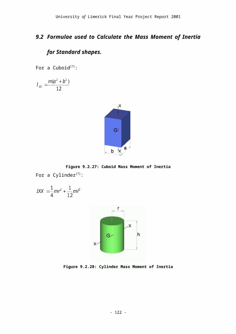
Figure 9.16.60 shows the resulting expansion for the metal parts and the contraction
for the carbon fibre part as calculated by ProMechanica.
Figure 9.16.60: Initial (Purple) and Deformed (Blue) Benchmark models for Carbon Fibre and Steel Respectively
The comparison of these results can be seen in Section 9.19. It indicates that the finite
element analysis has a high degree of accuracy, but that it does show some error due
to rounding during
calculations. This rounding
error is of the order of
6×10⁻¹⁰ %, and this becomes
an error of 2×10⁻⁶% when
these dimensions are used to
calculate the volume of the
deformed part.
Figure 9.16.61: The Queried X-Displacements in millimetres for the Steel Model (Values circled in red are maximum or minimum values).
However, even these error calculations suffer from rounding error as ProMechanica
outputs results to 14 significant places, and Microsoft Excel, the program used to
perform the error calculations operates to 15 significant places, causing some digits to

be lost as the total number of digits in each new dimension is 18, due to it being the
summation of 1000mm, the initial dimension, and x.xe-1, the change in the initial
dimension, which is a number with 14 significant digits.
Figure 9.16.61 shows the results given by ProMechanica when the query function was
used for the steel model. These results are exactly right except for some of the zero
values, as the full results from ProMechanica rounded to 6 decimal places will give
the same results as the theoretically calculated values.
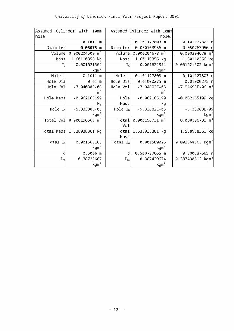
9.17Finite Element Analysis Run Summaries
9.17.1 Run Summary for Brass
Benchmark Test
--------------------------------------------------------Pro/MECHANICA STRUCTURE Version 22.3(305)Summary for Design Study "BenchmarkBrass"Mon Mar 12, 2001 17:19:13--------------------------------------------------------
Run Settings Memory allocation for block solver: 48.0
Pro/MECHANICA STRUCTURE Model Summary
Model Type: Three Dimensional
Points: 10 Edges: 29 Faces: 32
Springs: 0 Masses: 0 Beams: 0 Shells: 0 Solids: 12
Elements: 12
--------------------------------------------------------
Standard Design Study
Description: Benchmark Test of Steel Cylinder to confirm its behaviour under 25 degree temperature rise.
Static Analysis "BenchmarkBrass":
Convergence Method: Multiple-Pass Adaptive Plotting Grid: 10
Convergence Loop Log: (17:19:14)
>> Pass 1 <<Calculating Element Equations (17:19:14)Total Number of Equations: 22Maximum Edge Order: 1Solving Equations (17:19:15)Post-Processing Solution (17:19:15)Calculating Disp and Stress Results (17:19:15)Checking Convergence (17:19:17)
Elements Not Converged: 12 Edges Not Converged: 29 Measure Convergence: 100.0% Local Disp/Energy Index: 100.0% Global RMS Stress Index: 100.0%Resource Check (17:19:17) Elapsed Time (sec): 6.13 CPU Time (sec): 4.06 Memory Usage (kb): 91504 Wrk Dir Dsk Usage (kb): 0
>> Pass 2 <<Calculating Element Equations (17:19:17)Total Number of Equations: 109Maximum Edge Order: 2Solving Equations (17:19:17)Post-Processing Solution (17:19:17)Calculating Disp and Stress Results (17:19:17)Checking Convergence (17:19:19) Elements Not Converged: 8 Edges Not Converged: 29 Measure Convergence: 12.0% Local Disp/Energy Index: 100.0% Global RMS Stress Index: 100.0%Resource Check (17:19:19) Elapsed Time (sec): 7.95 CPU Time (sec): 5.67 Memory Usage (kb): 92592 Wrk Dir Dsk Usage (kb): 0
>> Pass 3 <<Calculating Element Equations (17:19:19)Total Number of Equations: 292Maximum Edge Order: 3Solving Equations (17:19:19)Post-Processing Solution (17:19:19)Calculating Disp and Stress Results (17:19:20)Checking Convergence (17:19:21) Elements Not Converged: 0 Edges Not Converged: 12 Measure Convergence: 1.3% Local Disp/Energy Index: 2.8% Global RMS Stress Index: 0.0% Resource Check (17:19:21) Elapsed Time (sec): 10.30 CPU Time (sec): 7.77 Memory Usage (kb): 92592 Wrk Dir Dsk Usage (kb): 0
>> Pass 4 << Calculating Element Equations (17:19:21) Total Number of Equations: 508 Maximum Edge Order: 4
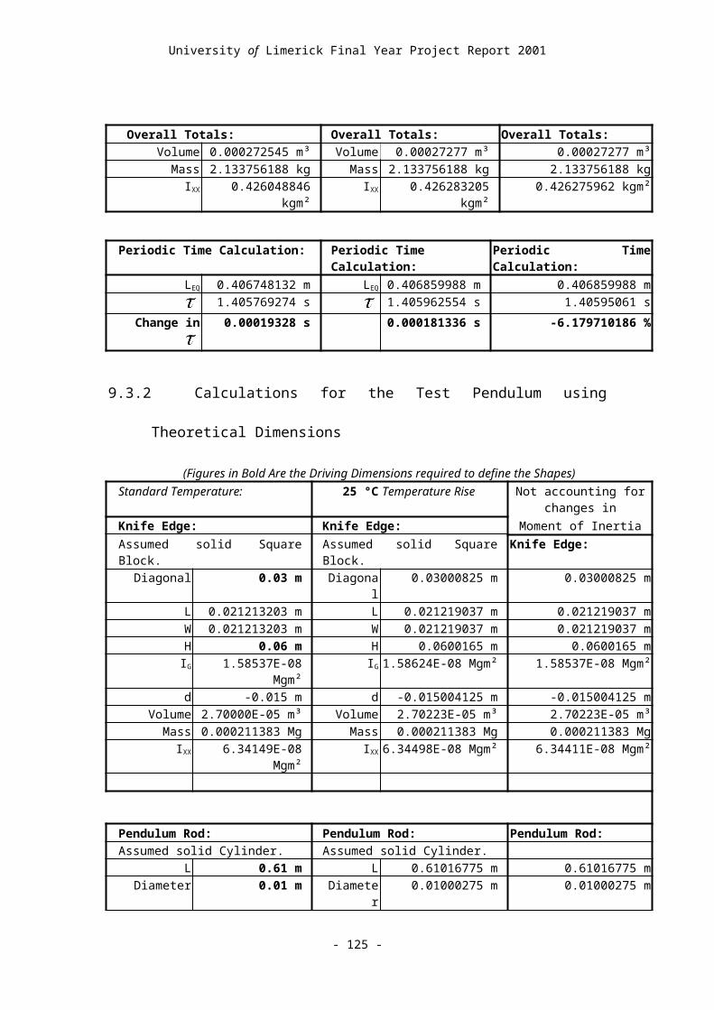
Solving Equations (17:19:22)Post-Processing Solution (17:19:22)Calculating Disp and Stress Results (17:19:22)Checking Convergence (17:19:24) Elements Not Converged: 0 Edges Not Converged: 0 Measure Convergence: 0.0% Local Disp/Energy Index: 0.0% Global RMS Stress Index: 0.0%
RMS Stress Error Estimates:
Load Set Stress Error % of Max Prin Str---------------- ------------ -----------------LoadSet1 6.58e-12 61.8% of 1.06e-11
Resource Check (17:19:25) Elapsed Time (sec): 13.98 CPU Time (sec): 11.00 Memory Usage (kb): 92592 Wrk Dir Dsk Usage (kb): 0
The analysis converged to within 1% on measures.
Total Mass of Model: 6.600958e+00
Total Cost of Model: 0.000000e+00
Mass Moments of Inertia about WCS Origin:
Ixx: 2.61278e+06Ixy: 7.83621e-07 Iyy: 8.24693e+05Ixz: 1.09139e-11 Iyz: -2.91038e-11 Izz: 2.61278e+06
Principal MMOI and Principal Axes Relative to WCS Origin:
Max Prin Mid Prin Min Prin2.61278e+06 2.61278e+06 8.24693e+05
WCS X: 0.00000e+00 1.00000e+00 0.00000e+00WCS Y: 0.00000e+00 0.00000e+00 1.00000e+00WCS Z: 1.00000e+00 0.00000e+00 0.00000e+00
Center of Mass Location Relative to WCS Origin: (-2.36813e-14, 5.00000e+02, 2.15285e-14)
Mass Moments of Inertia about the Center of Mass:
Ixx: 9.62544e+05Ixy: 7.83542e-07 Iyy: 8.24693e+05Ixz: 1.09139e-11 Iyz: 4.19504e-11 Izz: 9.62544e+05
Principal MMOI and Principal Axes Relative to COM:
Max Prin Mid Prin Min Prin9.62544e+05 9.62544e+05 8.24693e+05
WCS X: 0.00000e+00 1.00000e+00 0.00000e+00WCS Y: 0.00000e+00 0.00000e+00 1.00000e+00WCS Z: 1.00000e+00 0.00000e+00 0.00000e+00
Constraint Set: ConstraintSet1
Load Set: LoadSet1
Resultant Load on Model: in global X direction: 2.527572e-08 in global Y direction: 2.837242e-08 in global Z direction: -1.387300e-08
Measures:
Name Value Convergence -------------- ------------- -----------max_beam_bending: 0.000000e+00 0.0%max_beam_tensile: 0.000000e+00 0.0%max_beam_torsion: 0.000000e+00 0.0%max_beam_total: 0.000000e+00 0.0%max_disp_mag: 6.717514e-01 0.0%max_disp_x: 4.750000e-01 0.0%max_disp_y: 4.750000e-01 0.0%max_disp_z: 2.375000e-01 0.0%max_prin_mag: 1.064508e-11 1.9%max_rot_mag: 0.000000e+00 0.0%max_rot_x: 0.000000e+00 0.0%max_rot_y: 0.000000e+00 0.0%max_rot_z: 0.000000e+00 0.0%max_stress_prin: 1.064508e-11 6.3%max_stress_vm: 6.540717e-12 52.8%max_stress_xx: -6.684177e-12 35.3%max_stress_xy: -7.414438e-13 9.5%max_stress_xz: -1.106589e-12 6.0%max_stress_yy: 1.058438e-11 14.3%max_stress_yz: -1.163393e-12 45.0%max_stress_zz: -5.687675e-12 87.4%min_stress_prin: -7.833536e-12 38.4%strain_energy: 6.519258e-09 71.4%Diameter: 4.750000e-01 0.0%Height: 4.750000e-01 0.0%
Analysis "BenchmarkBrass" Completed (17:19:25)
--------------------------------------------------------
Memory and Disk Usage:

Machine Type: Windows NT/x86 RAM Allocation for Solver (megabytes): 48.0
Total Elapsed Time (seconds): 14.19 Total CPU Time (seconds): 11.09 Maximum Memory Usage (kilobytes): 92592 Working Directory Disk Usage (kilobytes): 0
Results Directory Size (kilobytes): 1139 .\BenchmarkBrass
--------------------------------------------------------Run CompletedMon Mar 12, 2001 17:19:25--------------------------------------------------------
9.17.2 Run Summary for Carbon
Fibre Benchmark Test
--------------------------------------------------------Pro/MECHANICA STRUCTURE Version 22.3(305)Summary for Design Study "BenchMarkCF"Mon Mar 12, 2001 17:14:58--------------------------------------------------------
Run Settings Memory allocation for block solver: 48.0
Pro/MECHANICA STRUCTURE Model Summary
Model Type: Three Dimensional
Points: 10 Edges: 29 Faces: 32
Springs: 0 Masses: 0 Beams: 0 Shells: 0 Solids: 12
Elements: 12
--------------------------------------------------------
Standard Design Study
Description: Benchmark Test of Steel Cylinder to confirm its behaviour under 25 degree temperature rise.
Static Analysis "BenchMarkCF":
Convergence Method: Multiple-Pass Adaptive Plotting Grid: 10
Convergence Loop Log: (17:15:00)
>> Pass 1 <<Calculating Element Equations (17:15:00) Total Number of Equations: 22 Maximum Edge Order: 1Solving Equations (17:15:00)Post-Processing Solution (17:15:00)Calculating Disp and Stress Results (17:15:00)Checking Convergence (17:15:02) Elements Not Converged: 12 Edges Not Converged: 29 Measure Convergence: 100.0% Local Disp/Energy Index: 100.0% Global RMS Stress Index: 100.0%Resource Check (17:15:02) Elapsed Time (sec): 5.63 CPU Time (sec): 4.03 Memory Usage (kb): 91504 Wrk Dir Dsk Usage (kb): 0
>> Pass 2 <<Calculating Element Equations (17:15:02) Total Number of Equations: 109 Maximum Edge Order: 2Solving Equations (17:15:03)Post-Processing Solution (17:15:03)Calculating Disp and Stress Results (17:15:03)Checking Convergence (17:15:04) Elements Not Converged: 12 Edges Not Converged: 29 Measure Convergence: 11.3% Local Disp/Energy Index: 100.0% Global RMS Stress Index: 100.0%Resource Check (17:15:04) Elapsed Time (sec): 7.27 CPU Time (sec): 5.50 Memory Usage (kb): 92592 Wrk Dir Dsk Usage (kb): 0
>> Pass 3 <<Calculating Element Equations (17:15:04) Total Number of Equations: 292 Maximum Edge Order: 3Solving Equations (17:15:04)Post-Processing Solution (17:15:04)Calculating Disp and Stress Results (17:15:05)Checking Convergence (17:15:06) Elements Not Converged: 0 Edges Not Converged: 12 Measure Convergence: 1.3% Local Disp/Energy Index: 2.7% Global RMS Stress Index: 0.0%Resource Check (17:15:06) Elapsed Time (sec): 9.44 CPU Time (sec): 7.52

Memory Usage (kb): 92592 Wrk Dir Dsk Usage (kb): 0
>> Pass 4 <<Calculating Element Equations (17:15:06)Total Number of Equations: 508 Maximum Edge Order: 4Solving Equations (17:15:07)Post-Processing Solution (17:15:07)Calculating Disp and Stress Results (17:15:07)Checking Convergence (17:15:09) Elements Not Converged: 0 Edges Not Converged: 0 Measure Convergence: 0.0% Local Disp/Energy Index: 0.0% Global RMS Stress Index: 0.0%
RMS Stress Error Estimates:
Load Set Stress Error % of Max Prin Str---------------- ------------ -----------------LoadSet1 5.19e-14 62.1% of 8.35e-14
Resource Check (17:15:10) Elapsed Time (sec): 12.78 CPU Time (sec): 10.77 Memory Usage (kb): 92592 Wrk Dir Dsk Usage (kb): 0
The analysis converged to within 1% on measures.
Total Mass of Model: 2.669545e-01
Total Cost of Model: 0.000000e+00
Mass Moments of Inertia about WCS Origin:
Ixx: 1.05666e+05 Ixy: 3.16900e-08 Iyy: 3.33521e+04 Ixz: 0.00000e+00 Iyz: 0.00000e+00 Izz: 1.05666e+05
Principal MMOI and Principal Axes Relative to WCS Origin:
Max Prin Mid Prin Min Prin1.05666e+05 1.05666e+05 3.33521e+04
WCS X: 0.00000e+00 1.00000e+00 0.00000e+00WCS Y: 0.00000e+00 0.00000e+00 1.00000e+00WCS Z: 1.00000e+00 0.00000e+00 0.00000e+00
Center of Mass Location Relative to WCS Origin: (-1.66354e-14, 5.00000e+02, 2.32895e-14)
Mass Moments of Inertia about the Center of Mass:
Ixx: 3.89270e+04 Ixy: 3.16878e-08 Iyy: 3.33521e+04Ixz: -1.03426e-28 Iyz: 3.10862e-12 Izz: 3.89270e+04
Principal MMOI and Principal Axes Relative to COM:
Max Prin Mid Prin Min Prin3.89270e+04 3.89270e+04 3.33521e+04
WCS X: 0.00000e+00 1.00000e+00 0.00000e+00 WCS Y: 0.00000e+00 0.00000e+00 1.00000e+00 WCS Z: 1.00000e+00 0.00000e+00 0.00000e+00
Constraint Set: ConstraintSet1
Load Set: LoadSet1
Resultant Load on Model: in global X direction: -1.219896e-10 in global Y direction: -2.362952e-11 in global Z direction: 2.339130e-10
Measures:
Name Value Convergence-------------- ------------- -----------max_beam_bending: 0.000000e+00 0.0%max_beam_tensile: 0.000000e+00 0.0%max_beam_torsion: 0.000000e+00 0.0%max_beam_total: 0.000000e+00 0.0% max_disp_mag: 2.828427e-02 0.0% max_disp_x: -2.000000e-02 0.0% max_disp_y: -2.000000e-02 0.0% max_disp_z: 1.000000e-02 0.0% max_prin_mag: 8.353739e-14 48.4% max_rot_mag: 0.000000e+00 0.0% max_rot_x: 0.000000e+00 0.0% max_rot_y: 0.000000e+00 0.0% max_rot_z: 0.000000e+00 0.0% max_stress_prin: 8.353739e-14 85.4% max_stress_vm: 2.172273e-14 33.1% max_stress_xx: 8.126304e-14 57.8% max_stress_xy: -4.941541e-15 56.3% max_stress_xz: -4.390926e-15 42.7% max_stress_yy: 7.850041e-14 45.2% max_stress_yz: -3.153819e-15 45.7% max_stress_zz: 6.927426e-14 50.0% min_stress_prin: -3.685547e-14 16.9% strain_energy: 3.751666e-12 54.5% Diameter: -2.000000e-02 0.0% Height: -2.000000e-02 0.0%

Analysis "BenchMarkCF" Completed (17:15:10)
--------------------------------------------------------Memory and Disk Usage:
Machine Type: Windows NT/x86 RAM Allocation for Solver (megabytes): 48.0
Total Elapsed Time (seconds): 12.95 Total CPU Time (seconds): 10.86 Maximum Memory Usage (kilobytes): 92592 Working Directory Disk Usage (kilobytes): 0
Results Directory Size (kilobytes): 1138 .\BenchMarkCF
--------------------------------------------------------Run CompletedMon Mar 12, 2001 17:15:10--------------------------------------------------------
9.17.3 Run Summary for Steel
Benchmark Test
--------------------------------------------------------Pro/MECHANICA STRUCTURE Version 22.3(305)Summary for Design Study "BenchmarkSteel"Mon Mar 12, 2001 17:12:15--------------------------------------------------------
Run Settings Memory allocation for block solver: 48.0
Pro/MECHANICA STRUCTURE Model Summary
Model Type: Three Dimensional
Points: 10 Edges: 29 Faces: 32
Springs: 0 Masses: 0 Beams: 0 Shells: 0 Solids: 12
Elements: 12
--------------------------------------------------------
Standard Design Study
Description:Benchmark Test of Steel Cylinder to confirm its behaviour under 25 degree temperature rise.
Static Analysis "BenchmarkSteel":
Convergence Method: Multiple-Pass Adaptive Plotting Grid: 10
Convergence Loop Log: (17:12:16)
>> Pass 1 <<Calculating Element Equations (17:12:16) Total Number of Equations: 22 Maximum Edge Order: 1Solving Equations (17:12:16)Post-Processing Solution (17:12:16)Calculating Disp and Stress Results (17:12:16)Checking Convergence (17:12:18) Elements Not Converged: 12 Edges Not Converged: 29 Measure Convergence: 100.0% Local Disp/Energy Index: 100.0% Global RMS Stress Index: 100.0%Resource Check (17:12:18) Elapsed Time (sec): 4.80 CPU Time (sec): 4.02 Memory Usage (kb): 91504 Wrk Dir Dsk Usage (kb): 0
>> Pass 2 <<Calculating Element Equations (17:12:18) Total Number of Equations: 109 Maximum Edge Order: 2Solving Equations (17:12:18)Post-Processing Solution (17:12:18)Calculating Disp and Stress Results (17:12:18)Checking Convergence (17:12:19) Elements Not Converged: 12 Edges Not Converged: 29 Measure Convergence: 10.9% Local Disp/Energy Index: 100.0% Global RMS Stress Index: 100.0%Resource Check (17:12:19) Elapsed Time (sec): 6.34 CPU Time (sec): 5.53 Memory Usage (kb): 92592 Wrk Dir Dsk Usage (kb): 0
>> Pass 3 <<Calculating Element Equations (17:12:19) Total Number of Equations: 292 Maximum Edge Order: 3Solving Equations (17:12:20)Post-Processing Solution (17:12:20)Calculating Disp and Stress Results (17:12:20)Checking Convergence (17:12:21) Elements Not Converged: 0 Edges Not Converged: 12
Measure Convergence: 1.3% Local Disp/Energy Index: 2.7% Global RMS Stress Index: 0.0%Resource Check (17:12:21) Elapsed Time (sec): 8.38 CPU Time (sec): 7.50 Memory Usage (kb): 92592 Wrk Dir Dsk Usage (kb): 0
>> Pass 4 <<Calculating Element Equations (17:12:21) Total Number of Equations: 508 Maximum Edge Order: 4Solving Equations (17:12:22)Post-Processing Solution (17:12:22)Calculating Disp and Stress Results (17:12:22)Checking Convergence (17:12:24) Elements Not Converged: 0 Edges Not Converged: 0 Measure Convergence: 0.0% Local Disp/Energy Index: 0.0% Global RMS Stress Index: 0.0%
RMS Stress Error Estimates:
Load Set Stress Error % of Max Prin Str---------------- ------------ -----------------LoadSet1 1.48e-11 61.2% of 2.41e-11
Resource Check (17:12:25) Elapsed Time (sec): 11.86 CPU Time (sec): 10.67 Memory Usage (kb): 92592 Wrk Dir Dsk Usage (kb): 0
The analysis converged to within 1% on measures.
Total Mass of Model: 6.145665e+00
Total Cost of Model: 0.000000e+00
Mass Moments of Inertia about WCS Origin:
Ixx: 2.43257e+06 Ixy: 7.29633e-07 Iyy: 7.67811e+05 Ixz: 7.27596e-12 Iyz: -1.45519e-11 Izz: 2.43257e+06
Principal MMOI and Principal Axes Relative to WCS Origin:
Max Prin Mid Prin Min Prin2.43257e+06 2.43257e+06 7.67811e+05
WCS X: 0.00000e+00 1.00000e+00 0.00000e+00 WCS Y: 0.00000e+00 0.00000e+00 1.00000e+00
WCS Z: 1.00000e+00 0.00000e+00 0.00000e+00
Center of Mass Location Relative to WCS Origin: (-3.00604e-14, 5.00000e+02, 9.24935e-15)
Mass Moments of Inertia about the Center of Mass:
Ixx: 8.96153e+05 Ixy: 7.29541e-07 Iyy: 7.67811e+05Ixz: 7.27596e-12 Iyz: 1.38698e-11 Izz: 8.96153e+05
Principal MMOI and Principal Axes Relative to COM:
Max Prin Mid Prin Min Prin8.96153e+05 8.96153e+05 7.67811e+05
WCS X: 0.00000e+00 1.00000e+00 0.00000e+00 WCS Y: 0.00000e+00 0.00000e+00 1.00000e+00 WCS Z: 1.00000e+00 0.00000e+00 0.00000e+00
Constraint Set: ConstraintSet1
Load Set: LoadSet1
Resultant Load on Model: in global X direction: -4.841302e-08 in global Y direction: -3.551001e-08 in global Z direction: -3.806041e-08
Measures:
Name Value Convergence-------------- ------------- -----------max_beam_bending: 0.000000e+00 0.0%max_beam_tensile: 0.000000e+00 0.0%max_beam_torsion: 0.000000e+00 0.0%max_beam_total: 0.000000e+00 0.0% max_disp_mag: 3.889087e-01 0.0% max_disp_x: 2.750000e-01 0.0% max_disp_y: 2.750000e-01 0.0% max_disp_z: 1.375000e-01 0.0%max_prin_mag: -2.411673e-11 51.5% max_rot_mag: 0.000000e+00 0.0% max_rot_x: 0.000000e+00 0.0% max_rot_y: 0.000000e+00 0.0% max_rot_z: 0.000000e+00 0.0% max_stress_prin: 7.041881e-12 23.1% max_stress_vm: 7.461390e-12 12.3% max_stress_xx: -1.966355e-11 52.2% max_stress_xy: -9.968400e-13 44.7% max_stress_xz: 9.036722e-13 78.4% max_stress_yy: -2.408352e-11 52.4%

max_stress_yz: 8.794603e-13 17.8% max_stress_zz: -2.004753e-11 72.5% min_stress_prin: -2.411673e-11 51.5% strain_energy: 1.024455e-08 77.3% Diameter: 2.750000e-01 0.0% Height: 2.750000e-01 0.0%
Analysis "BenchmarkSteel" Completed (17:12:25)
--------------------------------------------------------Memory and Disk Usage:
Machine Type: Windows NT/x86RAM Allocation for Solver (megabytes): 48.0
Total Elapsed Time (seconds): 12.05 Total CPU Time (seconds): 10.77 Maximum Memory Usage (kilobytes): 92592 Working Directory Disk Usage (kilobytes): 0
Results Directory Size (kilobytes): 1137 .\BenchmarkSteel
--------------------------------------------------------Run CompletedMon Mar 12, 2001 17:12:25--------------------------------------------------------

9.17.4 Run Summary for Split Block
and Spring Contact Analysis
--------------------------------------------------------Pro/MECHANICA STRUCTURE Version 22.3(305)Summary for Design Study "FinalContact"Tue Mar 06, 2001 17:32:35--------------------------------------------------------
Run Settings Memory allocation for block solver: 48.0
Pro/MECHANICA STRUCTURE Model Summary
Model Type: Three Dimensional
Points: 100 Edges: 347 Faces: 396
Springs: 0 Masses: 0 Beams: 0 Shells: 25 Solids: 149
Elements: 174
Contact Regions: 4
Links: 10
--------------------------------------------------------
Standard Design Study
Description:Contact Analysis of the brass split block interface with the steel suspension spring and its pin and rivet
Static Analysis "FinalContact":Contact Analysis
Convergence Method: Multiple-Pass Adaptive Plotting Grid: 4
Convergence Loop Log: (17:32:40)
>> Pass 1 <<Calculating Element Equations (17:32:41) Total Number of Equations: 324 Maximum Edge Order: 1Solving Equations (17:32:42) Load Increment 0 of 3 Load Factor: 0.00000e+00

Contact Area: 0.00000e+00Calculating Disp and Stress Results (17:32:45) Load Increment 1 of 3 Load Factor: 3.33333e-01 *Contact Area: 5.63673e+00Calculating Disp and Stress Results (17:32:54) Load Increment 2 of 3 Load Factor: 6.66667e-01 *Contact Area: 5.63673e+00Calculating Disp and Stress Results (17:33:00) Load Increment 3 of 3 Load Factor: 1.00000e+00 *Contact Area: 5.63673e+00
** Warning: Contact area is small in comparison to size of adjacent element edges for one or more contact regions for all load factors above marked with a "*". If you need pressure results near the contact regions, use single-pass adaptive convergence and select Localized Mesh Refinement.Calculating Disp and Stress Results (17:33:05)
Post-Processing Solution (17:33:07)Checking Convergence (17:33:07) Elements Not Converged: 174 Edges Not Converged: 347 Measure Convergence: 100.0% Local Disp/Energy Index: 100.0% Global RMS Stress Index: 100.0%Resource Check (17:33:07) Elapsed Time (sec): 33.93 CPU Time (sec): 28.66 Memory Usage (kb): 83414 Wrk Dir Dsk Usage (kb): 26
>> Pass 2 <<Calculating Element Equations (17:33:09) Total Number of Equations: 1469 Maximum Edge Order: 2Solving Equations (17:33:09) Load Increment 0 of 3 Load Factor: 0.00000e+00 Contact Area: 0.00000e+00Calculating Disp and Stress Results (17:33:16) Load Increment 1 of 3 Load Factor: 3.33333e-01 *Contact Area: 5.15557e+00Calculating Disp and Stress Results (17:33:44) Load Increment 2 of 3 Load Factor: 6.66667e-01 *Contact Area: 5.15557e+00Calculating Disp and Stress Results (17:34:12) Load Increment 3 of 3 Load Factor: 1.00000e+00 *Contact Area: 5.15557e+00
** Warning: Contact area is small in comparison to size of adjacent element edges for one or more contact regions for all load
factors above marked with a "*". If you need pressure results near the contact regions, use single-pass adaptive convergence and select Localized Mesh Refinement.Calculating Disp and Stress Results (17:34:40)
Post-Processing Solution (17:34:41)Checking Convergence (17:34:41) Elements Not Converged: 89 Edges Not Converged: 264 Measure Convergence: 2.6% Local Disp/Energy Index: 100.0% Global RMS Stress Index: 0.8%Resource Check (17:34:41) Elapsed Time (sec): 128.43 CPU Time (sec): 121.35 Memory Usage (kb): 84502 Wrk Dir Dsk Usage (kb): 178
>> Pass 3 <<Calculating Element Equations (17:34:45) Total Number of Equations: 3542 Maximum Edge Order: 4Solving Equations (17:34:47) Load Increment 0 of 3 Load Factor: 0.00000e+00 Contact Area: 0.00000e+00Calculating Disp and Stress Results (17:35:10) Load Increment 1 of 3 Load Factor: 3.33333e-01 *Contact Area: 5.14344e+00Calculating Disp and Stress Results (17:36:00) Load Increment 2 of 3 Load Factor: 6.66667e-01 *Contact Area: 5.14344e+00Calculating Disp and Stress Results (17:36:51) Load Increment 3 of 3 Load Factor: 1.00000e+00 *Contact Area: 5.14344e+00
** Warning: Contact area is small in comparison to size of adjacent element edges for one or more contact regions for all load factors above marked with a "*". If you need pressure results near the contact regions, use single-pass adaptive convergence and select Localized Mesh Refinement.Calculating Disp and Stress Results (17:37:41)
Post-Processing Solution (17:37:43)Checking Convergence (17:37:43) Elements Not Converged: 43 Edges Not Converged: 0 Measure Convergence: 0.2% Local Disp/Energy Index: 100.0% Global RMS Stress Index: 0.7%
RMS Stress Error Estimates:
Load Set Stress Error % of Max Prin Str

---------------- ------------ -----------------LoadSet1 1.38e+00 5.0% of 2.77e+01
Resource Check (17:37:45) Elapsed Time (sec): 312.21 CPU Time (sec): 299.47 Memory Usage (kb): 85078 Wrk Dir Dsk Usage (kb): 3619
The analysis converged to within 1% on measures.
Total Mass of Model: 1.339851e-06
Total Cost of Model: 0.000000e+00
Mass Moments of Inertia about WCS Origin:
Ixx: 2.66867e-04 Ixy: 3.62645e-05 Iyy: 9.77388e-06 Ixz: 2.97260e-12 Iyz: -1.03839e-11 Izz: 2.75649e-04
Principal MMOI and Principal Axes Relative to WCS Origin:
Max Prin Mid Prin Min Prin2.75649e-04 2.71884e-04 4.75647e-06
WCS X: 4.05726e-07 9.90564e-01 -1.37050e-01WCS Y: 1.62841e-08 1.37050e-01 9.90564e-01WCS Z: 1.00000e+00 -4.04130e-07 3.94745e-08
Center of Mass Location Relative to WCS Origin: (-2.00000e+00, 1.35331e+01, 4.83005e-07)
Mass Moments of Inertia about the Center of Mass:
Ixx: 2.14812e-05 Ixy: 7.50588e-12 Iyy: 4.41450e-06Ixz: 1.67829e-12 Iyz: -1.62595e-12 Izz: 2.49039e-05
Principal MMOI and Principal Axes Relative to COM:
Max Prin Mid Prin Min Prin2.49039e-05 2.14812e-05 4.41450e-06
WCS X: 4.90337e-07 1.00000e+00 -4.39797e-07WCS Y: -7.93552e-08 4.39797e-07 1.00000e+00WCS Z: 1.00000e+00 -4.90337e-07 7.93554e-08
Constraint Set: ConstraintSet1
Load Set: LoadSet1
Resultant Load on Model: in global X direction: -1.079579e-12 in global Y direction: -8.966466e-12 in global Z direction: 1.294446e-12
Measures:
Name Value Convergence-------------- ------------- ----------- contact_area: 5.143444e+00 0.2%contact_max_pres: 4.292490e+00 30.6%max_beam_bending: 0.000000e+00 0.0%max_beam_tensile: 0.000000e+00 0.0%max_beam_torsion: 0.000000e+00 0.0%max_beam_total: 0.000000e+00 0.0% max_disp_mag: 7.884895e-03 0.0% max_disp_x: 2.284773e-03 0.3% max_disp_y: 7.542785e-03 0.0% max_disp_z: -5.843065e-04 0.5% max_prin_mag: 2.773742e+01 9.1% max_rot_mag: 9.356744e-05 10.6% max_rot_x: -6.858245e-06 44.1% max_rot_y: -3.825938e-06 15.7% max_rot_z: -9.338629e-05 10.5% max_stress_prin: 2.773742e+01 9.1%max_stress_vm: 2.772074e+01 13.1% max_stress_xx: -5.235828e+00 76.3% max_stress_xy: -1.124145e+01 4.5% max_stress_xz: 6.339312e-01 3.9% max_stress_yy: 2.767054e+01 9.5% max_stress_yz: -1.341582e+00 11.4% max_stress_zz: -7.425485e+00 34.4% min_stress_prin: -1.630854e+01 9.9% strain_energy: 7.571377e-04 52.3% BlockDispl: 1.837009e-03 0.2%cntRgn_001cntArea: 1.142975e+00 0.8%cntRgn_001maxPres: 4.292490e+00 30.6%cntRgn_002cntArea: 1.434668e+00 0.0%cntRgn_002maxPres: 2.604255e+00 56.2%cntRgn_003cntArea: 1.139767e+00 1.3%cntRgn_003maxPres: 4.292490e+00 30.6%cntRgn_004cntArea: 1.426034e+00 0.8%cntRgn_004maxPres: 2.604255e+00 56.2%
Analysis "FinalContact" Completed (17:37:45)
--------------------------------------------------------
Memory and Disk Usage:
Machine Type: Windows NT/x86RAM Allocation for Solver (megabytes): 48.0
Total Elapsed Time (seconds): 312.44
Total CPU Time (seconds): 299.67 Maximum Memory Usage (kilobytes): 85078 Working Directory Disk Usage (kilobytes): 3619
Results Directory Size (kilobytes): 2723 .\FinalContact
Maximum Data Base Working File Sizes (kilobytes):
1024 .\FinalContact.tmp\gapel1.bas 2048 .\FinalContact.tmp\kel1.bas
--------------------------------------------------------Run CompletedTue Mar 06, 2001 17:37:45--------------------------------------------------------
9.18Finite Element Analysis Report Files
The following are the Reports produced by ProMechanica indicating the
displacements of the points set as measures in the Benchmark Test Models and the
Contact analysis Model.
9.18.1 Carbon Fibre Displacement Results
# MECHANICA Graph Report File
# Product: Pro/MECHANICA(R) STRUCTURE 22.3(305)
# Created: 03/12/01 at 17:17:25
# Machine: i486_nt
# Graphics: opengl/'window0'
# Language: (usascii)
# title = MeasuresCF - ..\..\..\..\WINNT\Profiles\9731318\Desktop\BenchMarkCF -
BenchMarkCF
# independent variable label = P Loop Pass
# dependent variable label = Height
# col data item
# 1 P Loop Pass
# 2 Height
# number of rows = 4
1.0000000000000E+000 -2.0629180595279E-002
2.0000000000000E+000 -1.9941110163927E-002
3.0000000000000E+000 -1.9999999552965E-002
4.0000000000000E+000 -1.9999999552965E-002

9.18.2 Brass Displacement Results
# MECHANICA Graph Report File
# Product: Pro/MECHANICA(R) STRUCTURE 22.3(305)
# Created: 03/12/01 at 17:20:30
# Machine: i486_nt
# Graphics: opengl/'window0'
# Language: (usascii)
# title = MeasuresBrass - ..\..\..\..\WINNT\Profiles\9731318\Desktop\BenchmarkBrass
- BenchmarkBrass
# independent variable label = P Loop Pass
# dependent variable label = Height
# col data item
# 1 P Loop Pass
# 2 Height
# number of rows = 4
1.0000000000000E+000 4.9085310101509E-001
2.0000000000000E+000 4.7341009974480E-001
3.0000000000000E+000 4.7499999403954E-001
4.0000000000000E+000 4.7499999403954E-001
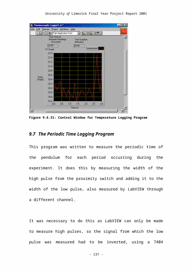
9.18.3 Steel Displacement Results
# MECHANICA Graph Report File
# Product: Pro/MECHANICA(R) STRUCTURE 22.3(305)
# Created: 03/12/01 at 17:16:24
# Machine: i486_nt
# Graphics: opengl/'window0'
# Language: (usascii)
# title = Measures - ..\..\..\..\WINNT\Profiles\9731318\Desktop\BenchmarkSteel -
BenchmarkSteel
# independent variable label = P Loop Pass
# dependent variable label = Height
# col data item
# 1 P Loop Pass
# 2 Height
# number of rows = 4
1.0000000000000E+000 2.8332769870758E-001
2.0000000000000E+000 2.7425619959831E-001
3.0000000000000E+000 2.7500000596046E-001
4.0000000000000E+000 2.7500000596046E-001
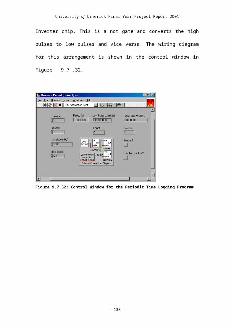
9.18.4 Result for displacement of a point at the end of the Split Block
calculated using Finite Element Analysis
# MECHANICA Graph Report File
# Product: Pro/MECHANICA(R) STRUCTURE 22.3(305)
# Created: 03/06/01 at 23:09:11
# Machine: i486_nt
# Graphics: opengl/'window0'
#
# Language: (usascii)
#
# title = Measure - ceason\topspring\FinalContact - FinalContact
#
# independent variable label = P Loop Pass
# dependent variable label = BlockDispl
#
# col data item
# 1 P Loop Pass
# 2 BlockDispl
#
# number of rows = 3
1.0000000000000E+000 1.8873759545386E-003
2.0000000000000E+000 1.8402209971100E-003
3.0000000000000E+000 1.8370089819655E-003

9.19Summary of Displacement Calculation Results
Displacement Benchmark Test For Steel
Coefficient of Expansion: 1.1E-05 m/m°C
From Finite Element Analysis: Manual Calculation:
Model: Cylinder Change in T 25°C
Dimensions: Dimensions:
Diameter 1000 mm Diameter 1000 mm
H 1000 mm H 1000 mm
Volume: 785398163.4 mm³ Volume: 785398163.4 mm³
In millilitres 785398.1634 ml In millilitres 785398.1634 ml
Deformed Dimensions: Deformed Dimensions: % Error
Diameter 1000.27500000596 mm Diameter 1000.275 mm 5.95885E-10
H 1000.27500000596 mm H 1000.275 mm 5.95885E-10
Volume: 786046295.1 mm³ Volume: 786046295.1 mm³ 1.78765E-09
In millilitres 786046.2951 ml In millilitres 786046.2951 ml 1.78765E-09
Change in Vol: 648131.7024 mm³ Change in Vol: 648131.6883 mm³ 2.16805E-06
In millilitres 648.1317024 ml In millilitres 648.1316883 ml 2.16804E-06
Displacement Benchmark Test For Brass
Coefficient of Expansion: 1.9E-05 m/m°C
From Finite Element Analysis: Manual Calculation:
Model: Cylinder Change in T 25°C
Dimensions: Dimensions:
Diameter 1000 mm Diameter 1000 mm
H 1000 mm H 1000 mm
Volume: 785398163.4 mm³ Volume: 785398163.4 mm³
In millilitres 785398.1634 ml In millilitres 785398.1634 ml
Deformed Dimensions: Deformed Dimensions: % Error
Diameter 1000.47499999403 mm Diameter 1000.475 mm -5.95766E-10
H 1000.47499999403 mm H 1000.475 mm -5.95766E-10
Volume: 786517887.5 mm³ Volume: 786517887.5 mm³ -1.7873E-09
In millilitres 786517.8875 ml In millilitres 786517.8875 ml -1.78729E-09
Change in Vol: 1119724.069 mm³ Change in Vol: 1119724.083 mm³ -1.25543E-06
In millilitres 1119.724069 ml In millilitres 1119.724083 ml -1.25544E-06
Displacement Benchmark Test For Carbon Fibre
Coefficient of Expansion: -8.0E-07 m/m°C
From Finite Element Analysis: Manual Calculation:
Model: Cylinder Change in T 25°C
Dimensions: Dimensions:
Diameter 1000 mm Diameter 1000 mm
H 1000 mm H 1000 mm
Volume: 785398163.4 mm³ Volume: 785398163.4 mm³
In millilitres 785398.1634 ml In millilitres 785398.1634 ml
Deformed Dimensions: Deformed Dimensions: % Error
Diameter 999.98000000045 mm Diameter 999.98 mm 4.47026E-11
H 999.98000000045 mm H 999.98 mm 4.47026E-11
Volume: 785351040.5 mm³ Volume: 785351040.5 mm³ 1.34123E-10
In millilitres 785351.0405 ml In millilitres 785351.0405 ml 1.34123E-10
Change in Vol: -47122.94628 mm³ Change in Vol: -47122.9473 mm³ -2.23529E-06
In millilitres -47.12294628 ml In millilitres -47.12294733 ml -2.23518E-06
Nomenclature:
T Temperature
H Height of Cylinder
Vol Volume
Units are as given with each value.
Conclusion: Finite Element Analysis Results Agree very closely with theoretical
answers, but rounding error affects some zero values.

9.20Raw Data from Low Temperature Tests
Time Temperature Time Period Time Temperature Time Period Time Temperature Time Period
0 17.065 7.0701959 707019.59 0 17.554 7.0702388 707023.88 0 11.768 7.070678 707067.82
5 17.798 14.1404117 707021.58 5 18.091 14.1399361 706969.73 5 9.985 14.13997 706928.68
10 17.114 21.210431 707001.93 10 12.524 21.2093337 706939.76 10 17.139 21.20896 706899.34
15 13.574 28.2803727 706994.17 15 17.7 28.278576 706924.23 15 17.139 28.27778 706881.88
20 10.229 35.3500917 706971.9 20 15.552 35.347603 706902.7 20 18.188 35.34637 706859.59
25 17.798 42.41972 706962.83 25 16.919 42.4164963 706889.33 25 18.97 42.41485 706847.66
30 18.799 49.4891671 706944.71 30 4.443 49.4852193 706872.3 30 14.014 49.48312 706827.24
35 19.458 56.5585544 706938.73 35 17.651 56.5538526 706863.33 35 16.528 56.55128 706816.02
40 18.701 63.62775 706919.56 40 15.063 63.6222708 706841.82 40 17.48 63.61927 706798.82
45 17.993 70.696897 706914.7 45 18.14 70.6905929 706832.21 45 18.115 70.68721 706793.58
50 16.895 77.7658744 706897.74 50 14.966 77.7587648 706817.19 50 17.505 77.75497 706776.72
55 17.578 84.8348357 706896.13 55 17.407 84.8268701 706810.53 55 9.351 84.82264 706767.1
60 16.846 91.9036348 706879.91 60 9.253 91.8947789 706790.88 60 18.262 91.89018 706753.34
65 14.844 98.9724017 706876.69 65 18.237 98.9626087 706782.98 65 17.871 98.95765 706747.44
70 17.847 106.0410141 706861.24 70 17.285 106.0303069 706769.82 70 17.627 106.025 706733.84
75 16.992 113.1096093 706859.52 75 17.261 113.097917 706761.01 75 18.115 113.0923 706729.94
80 16.675 120.1780275 706841.82 80 17.944 120.1653718 706745.48 80 16.724 120.1594 706715.74
85 17.798 127.2464589 706843.14 85 5.859 127.232749 706737.72 85 17.7 127.2266 706713.53
90 17.31 134.3147067 706824.78 90 19.165 134.2999556 706720.66 90 16.992 134.2936 706699.36

95 17.7 141.3829465 706823.98 95 18.481 141.3671309 706717.53 95 16.846 141.3605 706695.59
100 17.944 148.4510504 706810.39 100 17.48 148.4341555 706702.46 100 17.383 148.4274 706683.41
105 17.798 155.5191607 706811.03 105 17.578 155.5011704 706701.49 105 2.49 155.4942 706684.37
110 16.602 162.5871403 706797.96 110 17.725 162.5679876 706681.72 110 15.723 162.5609 706669
115 12.769 169.6551076 706796.73 115 17.407 169.6347675 706677.99 115 18.091 169.6276 706670.04
120 13.965 176.722955 706784.74 120 1.587 176.7014116 706664.41 120 10.889 176.6942 706659.48
125 17.92 183.7908523 706789.73 125 17.822 183.7680279 706661.63 125 16.846 183.7608 706657.93
130 16.992 190.8585831 706773.08 130 18.726 190.8344785 706645.06 130 17.285 190.8273 706647.9
135 16.479 197.9263397 706775.66 135 17.017 197.9008853 706640.68 135 17.163 197.8937 706645.04
140 16.87 204.9939692 706762.95 140 17.065 204.9671605 706627.52 140 18.628 204.9601 706636.04
145 18.018 212.0615826 706761.34 145 12.378 212.0334159 706625.54 145 12.036 212.0264 706636.22
150 16.772 219.1290629 706748.03 150 17.529 219.0994955 706607.96 150 17.505 219.0927 706626.82
155 17.505 226.1966302 706756.73 155 16.992 226.1655901 706609.46 155 16.968 226.1589 706624.8
160 16.333 233.2640408 706741.06 160 17.456 233.2315979 706600.78 160 18.408 233.2251 706617.23
165 17.603 240.331557 706751.62 165 16.943 240.2975804 706598.25 165 17.31 240.2914 706623.57
170 18.091 247.3988687 706731.17 170 15.747 247.3634287 706584.83 170 13.281 247.3575 706612.72
175 16.943 254.4662833 706741.46 175 17.31 254.4293066 706587.79 175 16.968 254.4236 706616.34
180 17.676 261.5335435 706726.02 180 17.212 261.4950096 706570.3 180 17.041 261.4897 706607.11
185 16.992 268.6008437 706730.02 185 17.041 268.5607523 706574.27 185 11.743 268.5558 706604.05
190 17.163 275.6680066 706716.29 190 17.041 275.6264053 706565.3 190 18.604 275.6217 706597.97
195 13.916 282.7352864 706727.98 195 17.358 282.6920026 706559.73 195 8.765 282.6878 706604.7
200 20.117 289.8023843 706709.79 200 17.212 289.7574582 706545.56 200 16.626 289.7537 706594.18
205 11.06 296.8694913 706710.7 205 17.969 296.8229326 706547.44 205 17.334 296.8197 706597.15
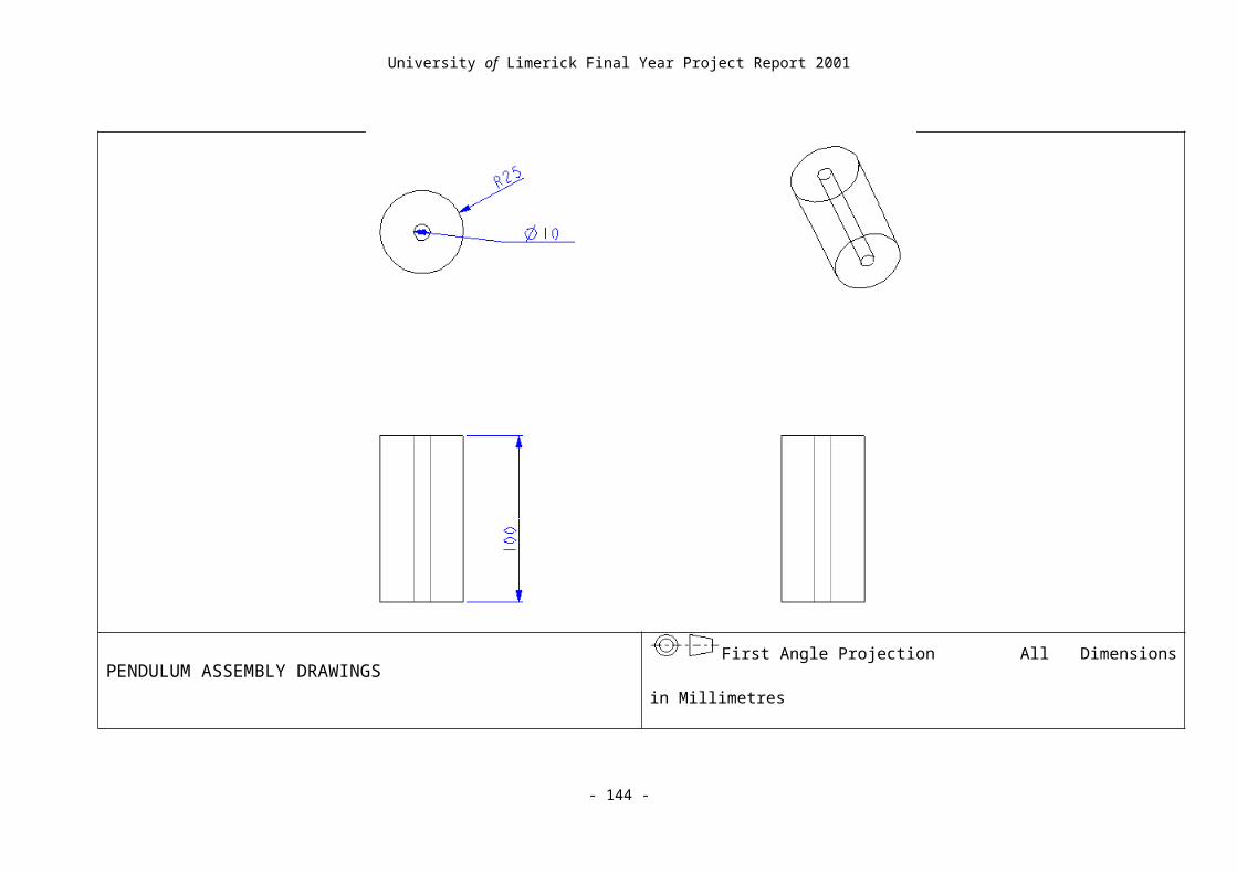
210 20.435 303.9364826 706699.13 210 15.723 303.8883007 706536.81 210 16.016 303.8856 706592.73
215 13.062 311.0036021 706711.95 215 17.285 310.9537432 706544.25 215 16.919 310.9516 706598.22
220 10.693 318.0705509 706694.88 220 18.286 318.019067 706532.38 220 16.553 318.0174 706583.25
225 7.056 325.1376144 706706.35 225 17.92 325.084456 706538.9 225 18.262 325.0834 706592.42
230 11.011 332.2045284 706691.4 230 16.797 332.1496987 706524.27 230 17.358 332.1492 706581.34
235 17.114 339.2715301 706700.17 235 17.212 339.2149195 706522.08 235 16.602 339.215 706585.52
240 17.432 346.3383442 706681.41 240 16.699 346.2800093 706508.98 240 17.212 346.2807 706571.52
245 17.725 353.4053125 706696.83 245 11.108 353.3450535 706504.42 245 17.163 353.3465 706575.7
250 17.407 360.4721223 706680.98 250 17.236 360.4099925 706493.9 250 17.383 360.4122 706566.58
255 17.505 367.5389625 706684.02 255 16.992 367.475082 706508.95 255 18.018 367.4779 706574.02
260 17.676 374.6056565 706669.4 260 8.936 374.5400092 706492.72 260 17.7 374.5435 706561.78
265 16.772 381.672428 706677.15 265 17.896 381.6050503 706504.11 265 12.891 381.6092 706570.41
270 18.701 388.7390036 706657.56 270 17.09 388.6699251 706487.48 270 18.066 388.6749 706563.68
275 16.992 395.8057915 706678.79 275 10.547 395.7348641 706493.9 275 8.765 395.7406 706570.06
280 17.383 402.8723742 706658.27 280 19.678 402.7997389 706487.48 280 16.919 402.8062 706560.73
285 17.041 409.9390007 706662.65 285 16.602 409.8646763 706493.74 285 16.235 409.8718 706565.94
290 17.041 417.0054936 706649.29 290 15.283 416.929361 706468.47 290 17.017 416.9375 706565.24
295 16.87 424.0721674 706667.38 295 17.456 423.9940572 706469.62 295 17.432 424.0031 706559.81
300 17.871 431.1386433 706647.59 300 17.651 431.0587728 706471.56 300 17.261 431.0686 706547.23
305 16.797 438.2052349 706659.16 305 2.002 438.1235225 706474.97 305 16.968 438.1341 706555.43
310 16.87 445.2717011 706646.62 310 17.993 445.188175 706465.25 310 17.603 445.1997 706558.61
315 17.432 452.3382828 706658.17 315 17.725 452.25293 706475.5 315 16.602 452.2652 706553.02
320 14.771 459.4046802 706639.74 320 17.48 459.3175305 706460.05 320 16.699 459.3306 706540.3
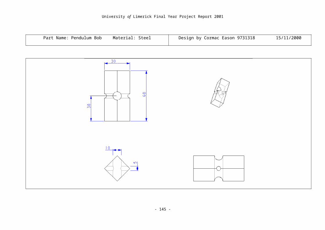
325 15.381 466.4712595 706657.93 325 17.285 466.3821719 706464.14 325 16.943 466.3962 706558.76
330 8.252 473.5376668 706640.73 330 16.504 473.4465827 706441.08 330 18.115 473.4617 706553.31
335 16.382 480.6041879 706652.11 335 17.7 480.5111205 706453.78 335 8.618 480.5274 706561.2
340 17.871 487.670554 706636.61 340 8.838 487.5756067 706448.62 340 18.604 487.5928 706542.13
345 17.7 494.7371224 706656.84 345 17.31 494.6401354 706452.87 345 7.544 494.6583 706554.99
350 17.603 501.8034607 706633.83 350 17.017 501.704514 706437.86 350 16.65 501.7237 706536.2
355 18.335 508.8700225 706656.18 355 16.699 508.7689269 706441.29 355 16.919 508.7892 706547.25
360 17.944 515.9363481 706632.56 360 17.944 515.8332569 706433 360 16.26 515.8545 706536.6
365 17.7 523.0028187 706647.06 365 16.919 522.8977845 706452.76 365 17.847 522.92 706551.32
370 17.847 530.0690691 706625.04 370 7.764 529.962077 706429.25 370 9.277 529.9854 706538.69
375 16.504 537.1355155 706644.64 375 17.236 537.0265552 706447.82 375 17.969 537.051 706554.11
380 17.139 544.2016591 706614.36 380 17.114 544.0909449 706438.97 380 17.09 544.1163 706535.48
385 18.457 551.2680494 706639.03 385 17.773 551.1553541 706440.92 385 17.139 551.1818 706545.24
390 17.456 558.3342801 706623.07 390 16.968 558.2196631 706430.9 390 18.115 558.2471 706536.4
395 17.554 565.400651 706637.09 395 17.871 565.2841591 706449.6 395 18.091 565.3126 706544.03
400 16.528 572.466856 706620.5 400 16.87 572.3483715 706421.24 400 14.868 572.3779 706532.86
405 16.626 579.5333806 706652.46 405 17.456 579.412888 706451.65 405 17.261 579.4434 706543.74
410 17.285 586.599598 706621.74 410 13.159 586.4771258 706423.78 410 14.966 586.5088 706541.47
415 17.603 593.6660251 706642.71 415 17.017 593.5416412 706451.54 415 10.547 593.5744 706559.42
420 17.773 600.7322417 706621.66 420 17.383 600.6059036 706426.24 420 17.383 600.6397 706533.84
425 19.214 607.7986635 706642.18 425 17.139 607.670261 706435.74 425 17.676 607.7052 706549.3
430 17.163 614.8649083 706624.48 430 18.921 614.734431 706417 430 8.521 614.7706 706541.53
435 16.187 621.9314991 706659.08 435 12.085 621.7988548 706442.38 435 17.7 621.8361 706547.76

440 15.283 628.9979043 706640.52 440 18.066 628.8632338 706437.9 440 4.321 628.9014 706530.94
445 12.549 636.0645616 706665.73 445 17.261 635.92749 706425.62 445 17.603 635.9669 706548.11
450 9.229 643.1310337 706647.21 450 17.09 642.9916028 706411.28 450 13.599 643.0323 706544.61
455 17.139 650.1976579 706662.42 455 17.09 650.0559166 706431.38 455 17.7 650.0979 706557.91
460 17.065 657.2638973 706623.94 460 14.941 657.1201108 706419.42 460 15.332 657.1632 706531.53
465 17.432 664.3306246 706672.73 465 17.31 664.1846388 706452.8 465 11.67 664.2288 706559.24
470 17.871 671.39685 706622.54 470 17.163 671.2487804 706414.16 470 17.383 671.2943 706545.93
475 16.919 678.4632877 706643.77 475 17.603 678.3131982 706441.78 475 17.065 678.36 706572.84
480 17.261 685.5295869 706629.92 480 17.163 685.377612 706441.38 480 17.187 685.4256 706556.7
485 18.286 692.5961185 706653.16 485 13.452 692.4422582 706464.62 485 17.822 692.4911 706549.62
490 17.334 699.6622493 706613.08 490 17.261 699.5067429 706448.47 490 17.798 699.5565 706545.88
495 17.578 706.7287543 706650.5 495 17.285 706.5714085 706466.56 495 16.919 706.6222 706566.02
500 19.116 713.795136 706638.17 500 17.139 713.6358595 706445.1 500 17.236 713.6877 706555.36
505 17.676 720.8618198 706668.38 505 16.821 720.7003759 706451.64 505 12.964 720.7535 706572.64
510 17.261 727.9281537 706633.39 510 17.139 727.7646472 706427.13 510 17.92 727.819 706555.86
515 18.14 734.9948203 706666.66 515 14.087 734.8293972 706475 515 15.039 734.8847 706566.86
520 17.456 742.0611714 706635.11 520 17.187 741.893764 706436.68 520 17.065 741.9503 706565.18
525 9.937 749.1280736 706690.22 525 17.139 748.958352 706458.8 525 10.229 749.0161 706577.41
530 16.797 756.194374 706630.04 530 16.724 756.0227119 706435.99 530 16.797 756.0817 706555.34
535 16.846 763.2612337 706685.97 535 17.48 763.0875119 706480 535 18.457 763.1475 706582.82
540 16.895 770.3277076 706647.39 540 17.725 770.1519578 706444.59 540 17.627 770.213 706551.35
545 17.725 777.3948382 706713.06 545 12.476 777.216697 706473.92 545 17.432 777.2792 706616.68
550 17.871 784.4614061 706656.79 550 17.017 784.2811724 706447.54 550 16.504 784.3447 706554.3
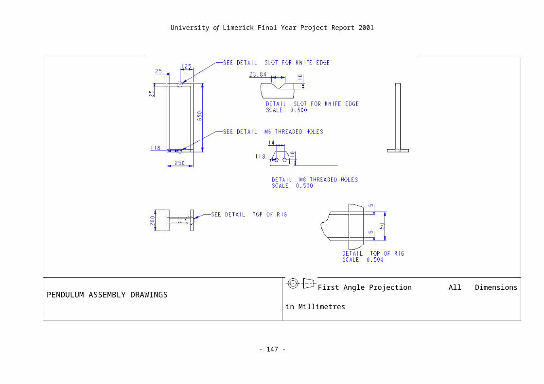
555 15.601 791.5285708 706716.47 555 17.212 791.346151 706497.86 555 17.383 791.4107 706601.23
560 14.258 798.5953014 706673.06 560 16.968 798.4105575 706440.65 560 9.961 798.4766 706582.23
565 12.744 805.6624871 706718.57 565 16.382 805.4754157 706485.82 565 18.359 805.5426 706609.02
570 7.983 812.729153 706666.59 570 18.286 812.5400549 706463.92 570 17.969 812.6085 706588.1
575 16.992 819.7963693 706721.63 575 8.203 819.6050363 706498.14 575 17.212 819.6747 706622.34
580 16.992 826.8629615 706659.22 580 16.968 826.669513 706447.67 580 17.358 826.7406 706587.83
585 16.821 833.930593 706763.15 585 17.896 833.7347021 706518.91 585 14.087 833.807 706632.98
590 17.871 840.9972205 706662.75 590 17.603 840.7992652 706456.31 590 17.944 840.8728 706588.22
595 16.968 848.0648222 706760.17 595 18.237 847.8644322 706516.7 595 17.798 847.9392 706633.29
600 17.529 855.1316764 706685.42 600 16.553 854.9290983 706466.61 600 16.968 855.0051 706590.62
605 18.164 862.1995841 706790.77 605 11.06 861.9945951 706549.68 605 16.943 862.0715 706645.54
610 17.773 869.2659973 706641.32 610 17.017 869.0594366 706484.15 610 13.965 869.1378 706622.79
615 17.651 876.3325814 706658.41 615 16.504 876.1247034 706526.68 615 17.603 876.2047 706692.14
620 17.09 883.3990776 706649.62 620 18.628 883.1894574 706475.4 620 17.847 883.2708 706615.08
625 17.017 890.4656379 706656.03 625 16.992 890.2552526 706579.52 625 17.725 890.3377 706689.74
630 16.992 897.5318379 706620 630 17.896 897.32021 706495.74 630 17.847 897.4041 706634.63
635 17.163 904.5982646 706642.67 635 17.334 904.386069 706585.9 635 17.285 904.4708 706672.72
640 17.09 Avg: 706717.3942 640 8.813 Avg: 706551.62 640 17.09 Avg: 706617.81
645 16.895 645 17.871 645 16.87
650 12.964 650 16.431 650 11.499 706628.94
655 15.259 655 17.847 655 17.798
660 16.504 660 17.847 660 18.579
665 16.968 665 17.407 665 18.237

670 16.821 670 18.213 670 16.748
675 17.334 675 17.114 675 17.383
680 18.14 680 14.917 680 17.31
685 17.261 685 16.748 685 14.136
690 17.822 690 18.018 690 18.433
695 16.846 695 17.261 695 18.384
700 17.065 700 17.163 700 19.702
705 16.87 705 17.31 705 18.335
710 17.554 710 16.724 710 16.528
715 17.358 715 17.041 715 17.285
720 15.527 720 10.01 720 17.92
725 14.38 725 17.236 725 16.992
730 13.794 730 17.456 730 14.502
735 16.821 735 17.383 735 17.09
740 17.358 740 17.065 740 14.38
745 17.09 745 13.452 745 16.846
750 17.603 750 17.773 750 17.358
755 17.407 755 17.773 755 17.334
760 18.262 760 17.749 760 17.847
765 17.285 765 10.864 765 16.943
770 9.839 770 16.943 770 17.603
775 17.969 775 17.969 775 17.969
780 16.968 780 17.334 780 17.603
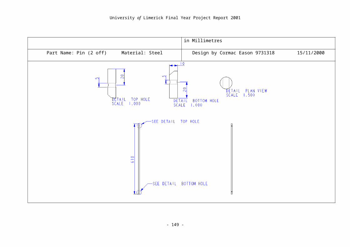
785 16.602 785 8.423 785 14.282
790 17.163 790 19.727 790 17.749
795 17.603 795 17.725 795 17.505
800 17.7 800 17.163 800 17.383
805 17.065 805 16.675 805 16.626
810 17.554 810 18.188 810 16.943
815 17.065 815 16.943 815 16.943
820 15.063 820 11.963 820 9.497
825 17.383 825 17.065 825 17.017
830 16.943 830 15.942 830 17.676
835 18.042 835 17.187 835 17.603
840 15.112 840 16.943 840 17.48
845 17.212 845 19.604 845 17.432
850 16.895 850 16.943 850 17.871
855 17.212 855 9.937 855 15.601
860 17.578 860 16.797 860 17.432
865 11.67 865 17.7 865 7.812
870 12.524 870 17.31 870 18.701
875 16.821 875 17.114 875 13.989
880 16.87 880 16.87 880 18.091
885 16.772 885 15.698 885 17.187
890 17.114 890 17.041 890 16.968
895 17.92 895 18.018 895 17.505
900 15.649 900 17.7 900 14.844
Avg: 16.56665193 Avg: 16.21781768 Avg: 16.18738674
9.21Raw Data from High Temperature Tests
Time Temperature Time Period Time + 90 Time Temperature Time Period Time Temperature Time Period
0 41.968 97.0649925 706499.25 90 0 42.432 97.06425 706424.9 0 45.679 97.06367 706367.5
5 41.284 104.1307935 706580.1 95 5 41.016 104.1293 706501.4 5 45.239 104.1282 706451.4
10 41.87 111.1957076 706491.41 100 10 39.697 111.1934 706414.4 10 45.923 111.1918 706361.7
15 41.895 118.2613518 706564.42 105 15 39.771 118.2583 706491.9 15 44.653 118.2562 706443.3
20 40.063 125.3261124 706476.06 110 20 39.258 125.3224 706408.5 20 35.62 125.3198 706355
25 36.06 132.3915932 706548.08 115 25 41.797 132.3873 706484.8 25 41.577 132.3842 706439.8
30 33.569 139.4562 706460.68 120 30 43.97 139.4512 706391.1 30 45.41 139.4476 706345.4
35 41.699 146.5215302 706533.02 125 35 40.161 146.5159 706475.7 35 45.361 146.512 706437
40 41.064 153.5859468 706441.66 130 40 40.601 153.5798 706390 40 44.653 153.5754 706338.4
45 41.992 160.6511688 706522.2 135 45 40.625 160.6445 706470.6 45 44.824 160.6397 706433.4
50 41.724 167.7154351 706426.63 140 50 40.259 167.7083 706373.5 50 37.378 167.7031 706338.1
55 41.382 174.7805322 706509.71 145 55 31.104 174.7729 706465.8 55 44.238 174.7674 706428.4
60 42.261 181.8446616 706412.94 150 60 41.797 181.8366 706366.4 60 44.58 181.8307 706327.7
65 40.698 188.9096476 706498.6 155 65 41.431 188.9012 706456 65 45.581 188.895 706429.5
70 41.577 195.9736206 706397.3 160 70 40.601 195.9647 706358.4 70 44.312 195.9582 706325.1
75 40.601 203.0384383 706481.77 165 75 21.606 203.0293 706452.7 75 44.531 203.0224 706419.5
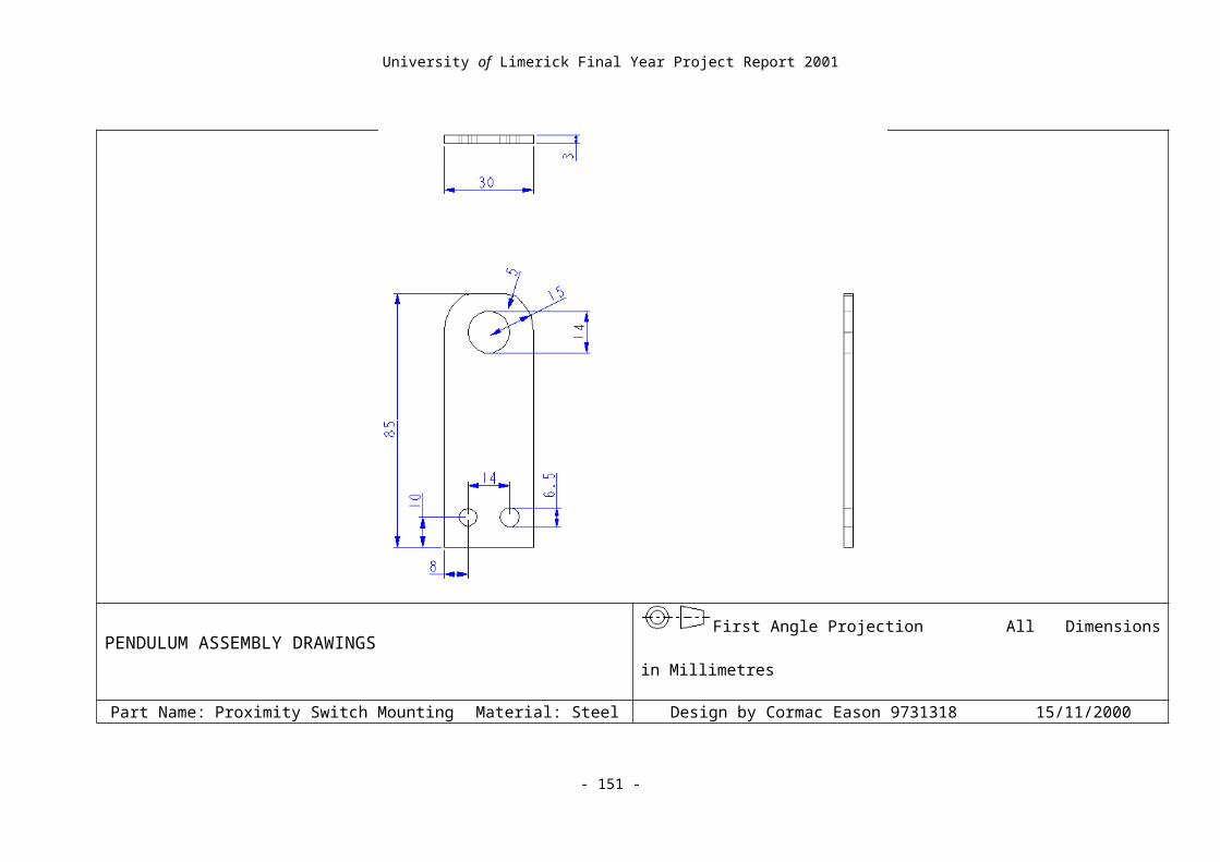
80 41.309 210.102284 706384.57 170 80 40.259 210.0928 706351.9 80 33.838 210.0856 706317.1
85 40.967 217.1669942 706471.02 175 85 40.625 217.1572 706444.9 85 43.164 217.1498 706417.2
90 41.504 224.230703 706370.88 180 90 40.527 224.2207 706344.1 90 44.629 224.2128 706308.4
95 40.991 231.295346 706464.3 185 95 41.553 231.2851 706446.2 95 44.409 231.277 706414.8
100 41.992 238.3588511 706350.51 190 100 31.03 238.3485 706335.8 100 44.556 238.3401 706306.8
105 41.113 245.4234177 706456.66 195 105 39.941 245.4129 706441.1 105 45.166 245.4042 706413.7
110 41.016 252.4869166 706349.89 200 110 41.675 252.4762 706329.3 110 39.429 252.4672 706299.8
115 40.576 259.5513494 706443.28 205 115 41.675 259.5405 706432.3 115 44.019 259.5313 706411.6
120 40.723 266.6147096 706336.02 210 120 38.159 266.6038 706324.9 120 43.921 266.5943 706297.6
125 41.138 273.6790603 706435.07 215 125 40.967 273.6681 706434.2 125 44.531 273.6583 706402.4
130 41.187 280.7422494 706318.91 220 130 35.205 280.7313 706319.7 130 44.824 280.7212 706293.7
135 40.186 287.8064923 706424.29 225 135 40.088 287.7956 706426.3 135 44.922 287.7853 706408
140 40.161 294.8696074 706311.51 230 140 40.845 294.8588 706318.3 140 33.789 294.8482 706288.1
145 41.846 301.9338516 706424.42 235 145 29.321 301.923 706422.6 145 38.062 301.9123 706406.5
150 40.649 308.9967878 706293.62 240 150 40.771 308.9861 706314.3 150 33.716 308.9751 706284.7
155 41.357 316.0609319 706414.41 245 155 40.796 316.0504 706424.4 155 36.304 316.0392 706405.7
160 40.601 323.1238027 706287.08 250 160 40.649 323.1134 706304.1 160 34.18 323.102 706282.1
165 41.602 330.1879065 706410.38 255 165 40.063 330.1776 706424 165 43.018 330.1661 706408.1
170 41.235 337.2506803 706277.38 260 170 26.489 337.2407 706300.5 170 43.091 337.2288 706272.6
175 40.527 344.3147043 706402.4 265 175 40.039 344.3049 706422.1 175 45.264 344.2929 706405.6
180 40.015 351.3774986 706279.43 270 180 39.771 351.3679 706297.9 180 44.849 351.3556 706273.8
185 40.479 358.4414483 706394.97 275 185 41.187 358.432 706418.8 185 43.677 358.4196 706400.3
190 41.602 365.5040809 706263.26 280 190 40.161 365.495 706295.2 190 45.337 365.4823 706267.5

195 40.674 372.5679436 706386.27 285 195 38.159 372.5592 706423.3 195 42.773 372.5463 706400.9
200 41.089 379.6305118 706256.82 290 200 34.448 379.6221 706285.5 200 43.53 379.609 706270.3
205 40.576 386.6944324 706392.06 295 205 40.137 386.6862 706415.6 205 43.457 386.6731 706410.1
210 40.405 393.7568414 706240.9 300 210 39.99 393.749 706280.6 210 45.386 393.7357 706260.9
215 40.381 400.8207 706385.86 305 215 35.083 400.8132 706419.5 215 44.092 400.7997 706402.5
220 36.157 407.8831444 706244.44 310 220 40.332 407.876 706277.8 220 44.922 407.8623 706257.6
225 40.601 414.9468678 706372.34 315 225 40.674 414.9402 706413.6 225 43.408 414.9263 706398.1
230 40.503 422.0092372 706236.94 320 230 39.6 422.0029 706275.9 230 43.042 421.9888 706254.6
235 39.819 429.0730722 706383.5 325 235 40.088 429.067 706409.3 235 39.16 429.0529 706411.3
240 40.503 436.1353136 706224.14 330 240 40.82 436.1297 706272 240 36.841 436.1154 706250.3
245 37.378 443.1990527 706373.91 335 245 39.99 443.1938 706407.8 245 43.408 443.1795 706409.8
250 40.552 450.2611849 706213.22 340 250 39.624 450.2565 706268.4 250 46.509 450.242 706244.7
255 40.283 457.3249256 706374.07 345 255 40.259 457.3207 706417.4 255 43.652 457.306 706405.6
260 40.576 464.38707 706214.44 350 260 33.96 464.3833 706263.7 260 44.312 464.3685 706247.4
265 40.21 471.4507961 706372.61 355 265 39.868 471.4475 706423.7 265 44.531 471.4325 706403.1
270 40.088 478.5128264 706203.03 360 270 40.112 478.5101 706259 270 44.067 478.4949 706239
275 31.396 485.5764642 706363.78 365 275 40.552 485.5743 706420.9 275 43.311 485.5591 706415.8
280 40.43 492.6385573 706209.31 370 280 39.673 492.6369 706259 280 44.287 492.6214 706233.7
285 40.015 499.7021792 706362.19 375 285 41.699 499.7012 706428.1 285 44.263 499.6856 706416.4
290 32.178 506.7640606 706188.14 380 290 31.177 506.7637 706253 290 43.848 506.7479 706234.2
295 40.356 513.8277116 706365.1 385 295 40.356 513.8279 706420.6 295 43.457 513.812 706410.9
300 37.769 520.8895083 706179.67 390 300 39.551 520.8904 706245.7 300 40.82 520.8743 706229
305 40.112 527.9531851 706367.68 395 305 40.43 527.9546 706424.7 305 40.527 527.9385 706418.3

310 41.016 535.0149586 706177.35 400 310 40.088 535.0171 706241.3 310 42.554 535.0008 706230.2
315 40.625 542.0785274 706356.88 405 315 30.078 542.0814 706438.5 315 34.741 542.065 706420.9
320 41.919 549.1402762 706174.88 410 320 39.624 549.1439 706244.6 320 29.932 549.1272 706221.8
325 31.86 556.2039876 706371.14 415 325 39.453 556.2083 706438.1 325 35.107 556.1916 706433
330 40.894 563.2656533 706166.57 420 330 39.795 563.2706 706233.2 330 41.382 563.2538 706221.6
335 40.088 570.3293424 706368.91 425 335 40.723 570.3349 706427.6 335 44.507 570.3181 706426.9
340 39.893 577.3909863 706164.39 430 340 43.066 577.3973 706240.8 340 44.312 577.3803 706223.3
345 41.528 584.4546068 706362.05 435 345 38.11 584.4617 706443 345 43.188 584.4447 706441.1
350 40.967 591.5161079 706150.11 440 350 37.109 591.524 706228 350 43.091 591.5069 706216.3
355 39.722 598.5798217 706371.38 445 355 30.127 598.5885 706447.5 355 41.553 598.5713 706444.1
360 41.602 605.6413065 706148.48 450 360 39.429 605.6508 706235.7 360 44.141 605.6334 706212.4
365 39.722 612.7050889 706378.24 455 365 40.015 612.7153 706446.2 365 35.01 612.6978 706438.2
370 40.186 619.7665664 706147.75 460 370 41.406 619.7776 706227.9 370 43.262 619.7599 706210.2
375 38.086 626.8302987 706373.23 465 375 39.551 626.8423 706468.9 375 43.481 626.8245 706458.4
380 31.396 633.8918165 706151.78 470 380 39.062 633.9045 706227.3 380 42.871 633.8866 706208.7
385 39.893 640.9556351 706381.86 475 385 40.234 640.9693 706481.8 385 44.189 640.9513 706472.9
390 41.504 648.0169975 706136.24 480 390 40.308 648.0316 706223.8 390 42.993 648.0135 706215.9
395 40.869 655.0808083 706381.08 485 395 41.04 655.0965 706488.3 395 43.164 655.0784 706497.1
400 40.503 662.1421925 706138.42 490 400 39.16 662.1586 706215.8 400 43.408 662.1405 706201.2
405 39.795 669.2062254 706403.29 495 405 39.551 669.2236 706498.4 405 45.166 669.2055 706500.4
410 39.136 676.2676013 706137.59 500 410 39.502 676.2857 706211.8 410 40.918 676.2675 706205.9
415 41.04 683.3318877 706428.64 505 415 39.624 683.3509 706515.7 415 44.385 683.3329 706537.8
420 34.619 690.3931886 706130.09 510 420 39.331 690.4131 706219 420 33.936 690.395 706211.5

425 40.063 697.4576993 706451.07 515 425 42.163 697.4782 706513.8 425 42.603 697.4602 706521.3
430 33.032 704.5189317 706123.24 520 430 39.478 704.5403 706205.8 430 33.618 704.5222 706201.8
435 27.222 711.5833629 706443.12 525 435 39.16 711.6059 706559.8 435 42.92 711.588 706579.2
440 39.551 718.6445666 706120.37 530 440 39.16 718.6679 706207.2 440 42.651 718.65 706198.1
445 38.843 725.7088807 706431.41 535 445 40.283 725.7338 706581.9 445 43.14 725.7162 706617.9
450 39.648 732.7698508 706097.01 540 450 39.136 732.7958 706200.7 450 43.433 732.7782 706199.6
455 39.453 739.8349862 706513.54 545 455 39.99 739.862 706622.1 455 43.506 739.8447 706654.8
460 40.894 746.8959944 706100.82 550 460 40.479 746.924 706202.3 460 42.847 746.9067 706195.3
465 40.088 753.9611236 706512.92 555 465 39.502 753.9909 706686.8 465 33.569 753.974 706729.8
470 39.819 761.0221298 706100.62 560 470 39.453 761.0528 706187.9 470 42.456 761.036 706196.8
475 40.698 768.0877268 706559.7 565 475 39.233 768.1207 706789.2 475 37.524 768.104 706805.1
480 40.747 775.1487438 706101.7 570 480 34.473 775.1825 706189.5 480 42.896 775.1659 706187.8
485 39.575 782.2150112 706626.74 575 485 39.746 782.2516 706909.4 485 30.737 782.2262 706027.2
490 39.331 789.2759916 706098.04 580 490 38.843 789.3134 706175.7 490 42.456 789.2881 706192.8
495 39.966 796.3434824 706749.08 585 495 39.355 796.3856 707216.8 495 42.871 Ignore 707815.80
500 39.819 803.4044412 706095.88 590 500 39.648 706192.19 Ignore 500 43.579 OL 1271137.23
505 40.479 810.473712 706927.08 595 505 40.43 169571.30 OL 505 42.676
510 39.575 817.5345874 706087.54 600 510 39.233 510 42.676
515 40.503 707736.71 605 515 38.94 515 42.48
520 39.6 Ignore Last 610 520 38.696 520 42.969
525 39.331 615 525 37.622 525 42.7
530 40.283 620 530 39.136 530 43.018
535 39.526 625 535 39.014 535 42.163
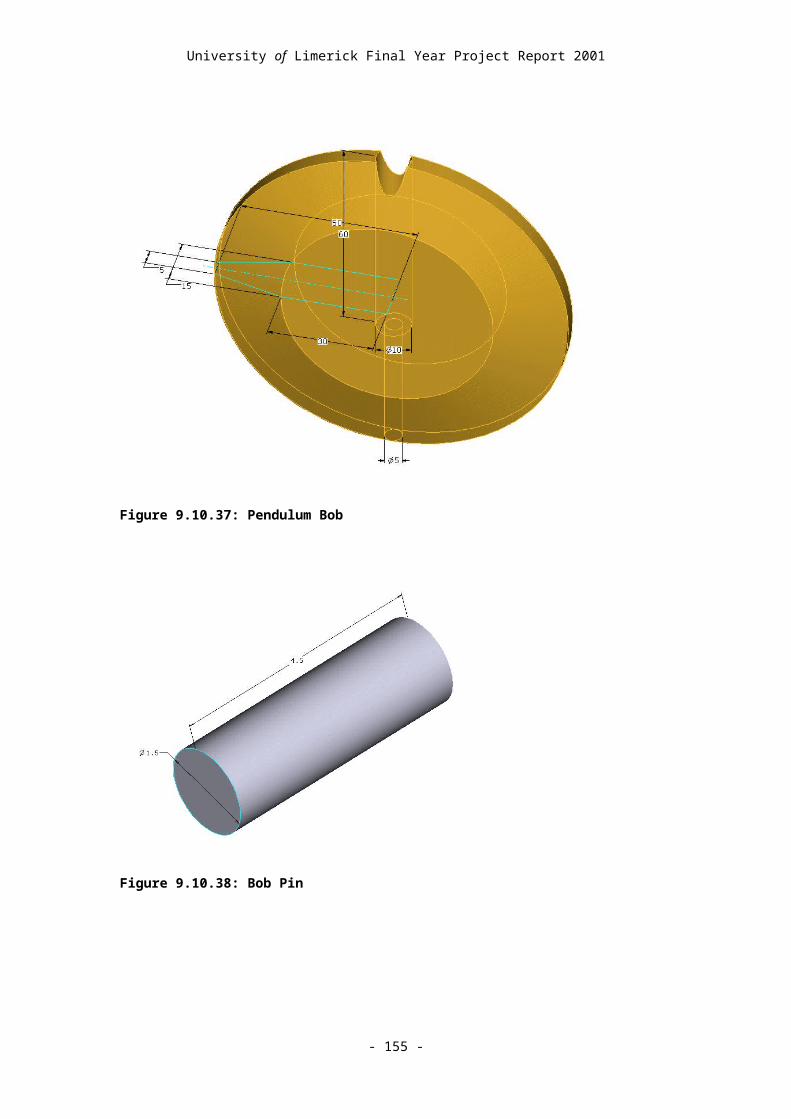
540 39.551 630 540 39.136 540 42.31
545 40.186 635 545 39.893 545 43.14
550 36.89 640 550 39.941 550 43.823
555 39.453 645 555 39.722 555 33.911
560 39.526 650 560 39.819 560 42.773
565 39.844 655 565 36.719 565 40.405
570 40.479 660 570 39.575 570 43.359
575 39.282 665 575 28.564 575 42.456
580 39.917 670 580 33.35 580 43.335
585 39.331 675 585 39.868 585 41.968
590 39.258 680 590 40.063 590 42.285
595 39.844 685 595 38.818 595 43.188
600 39.136 690 600 38.721 600 33.203
605 39.014 695 605 39.648 605 43.188
610 38.916 700 610 39.99 610 42.505
615 39.404 705 615 38.696 615 44.604
620 39.99 710 620 41.333 620 42.31
625 38.892 715 625 39.307 625 43.652
630 38.989 720 630 38.745 630 42.554
635 38.696 725 635 30.542 635 41.528
640 39.331 Avg: 706344.2596 730 640 37.573 Avg: 706385.6 640 42.261 Avg: 706351.6
645 37.671 735 645 31.738 645 42.505
650 38.843 740 650 38.867 650 42.603 706360.5
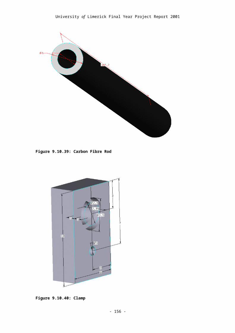
655 39.038 745 655 39.844 655 42.139
660 39.062 750 660 38.452 660 42.48
665 39.014 755 665 38.721 665 40.942
670 38.94 760 670 39.233 670 42.261
675 31.25 765 675 40.894 675 37.109
680 28.564 770 680 38.647 680 42.31
685 37.646 775 685 40.723 685 33.521
690 39.331 780 690 38.94 690 42.358
695 40.112 785 695 33.179 695 38.281
700 39.99 790 700 29.736 700 42.993
705 39.697 795 705 33.057 705 40.43
710 40.259 800 710 30.225 710 42.187
715 38.696 805 715 38.403 715 38.452
720 37.158 810 720 38.599 720 42.407
725 42.187 815 725 38.892 725 42.651
730 39.697 820 730 38.647 730 42.603
735 39.087 825 735 40.21 735 39.697
740 38.77 830 740 38.647 740 43.384
745 37.256 835 745 38.452 745 42.041
750 29.492 840 750 38.672 750 38.599
755 39.282 845 755 36.816 755 42.017
760 38.623 850 760 30.2 760 44.092
765 39.551 855 765 35.278 765 33.154
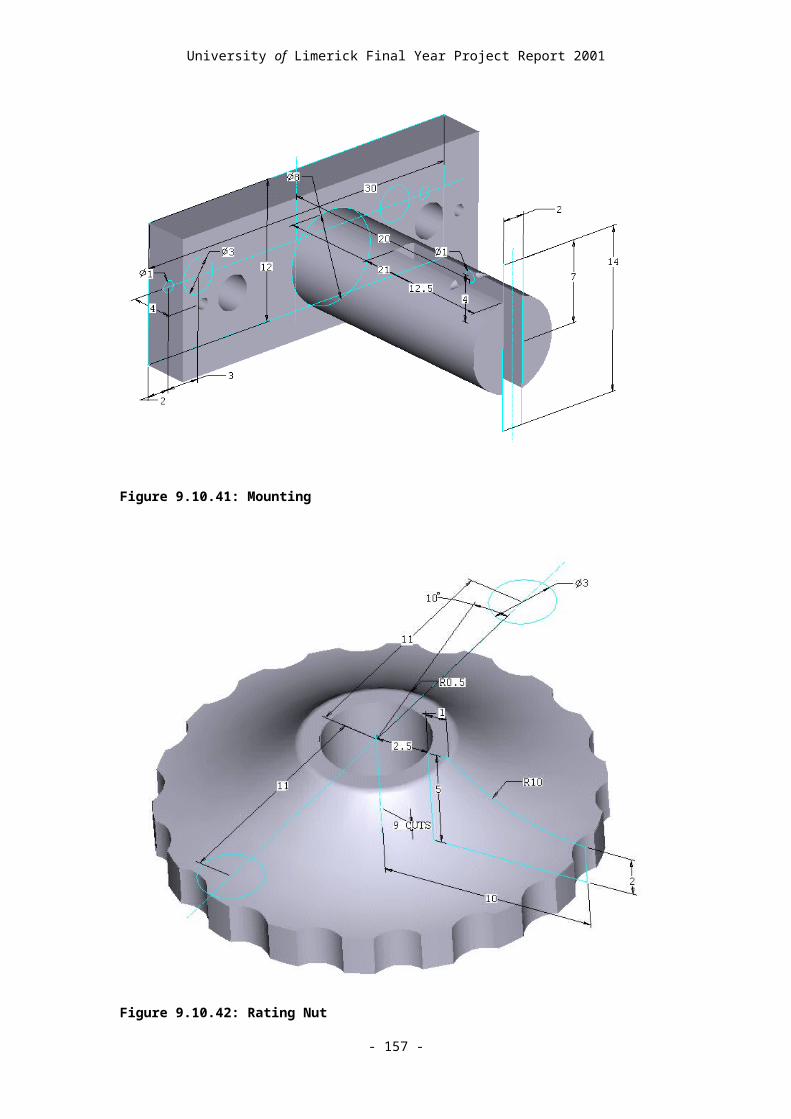
770 39.307 860 770 39.893 770 41.65
775 38.623 865 775 41.064 775 42.31
780 39.087 870 780 39.062 780 42.041
785 38.647 875 785 38.208 785 41.724
790 38.867 880 790 38.892 790 33.472
795 39.038 885 795 39.917 795 39.087
800 39.429 890 800 38.403 800 42.358
805 38.574 895 805 39.478 805 43.237
810 36.572 900 810 38.452 810 41.699
815 31.128 905 815 29.517 815 43.335
820 38.11 910 820 36.157 820 41.87
825 38.501 915 825 37.842 825 42.456
830 38.843 920 830 38.501 830 41.699
835 40.063 925 835 38.257 835 32.178
840 38.599 930 840 38.721 840 42.773
845 38.501 935
850 38.77 940
855 38.745 945
860 30.103 950
865 38.428 955
870 30.859 960
875 39.551 965
880 39.478 970
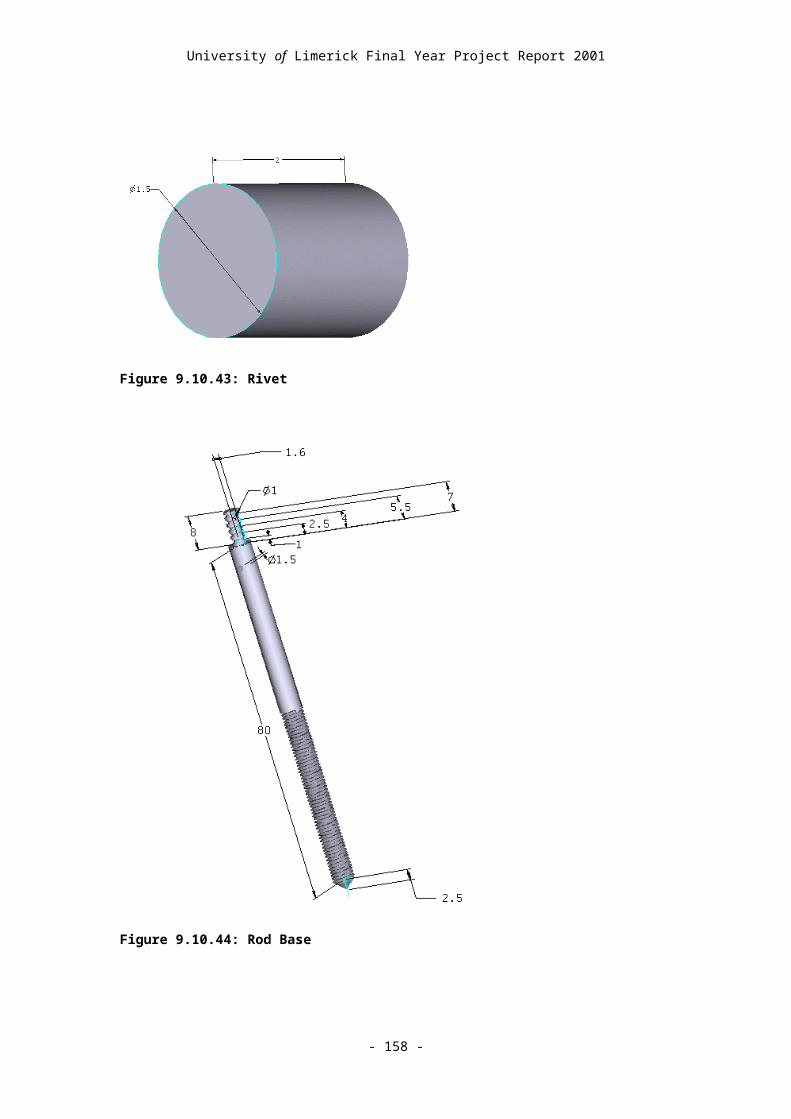
885 38.354 975
890 38.672 980
895 32.495 985
900 35.889 990
Avg: 39.15923204 Avg: 38.52971598 Avg: 41.77810059