MITRE

Sponsor: Federal Aviation Administration(FAA)

Dept. No.: F084Project No.: 0215BB02-ASOutcome No.: 2PBWP Reference: 2-6.1-1“Development of the FIM SPR and the FIMMOPS”

Approved for Public Release.This technical data was produced forthe U.S. Government under ContractNo. DTFAWA-10-C-00080, and issubject to the Rights in Technical Data—Noncommercial Items clause (DFARS)252.227-7013 (NOV 1995)c© 2015 The MITRE Corporation. All RightsReserved.

McLean, VA

MTR150184

MITRE TECHNICAL REPORT

Derivation of aPoint-Mass Aircraft Modelused for Fast-Time Simulation

MITRE Technical Report

Dr. Lesley A. Weitz

April 2015

Approved By:

Robert C. Strain, Department Head Date

Elida C. Smith, Outcome Leader Date

AbstractThis document describes a closed-loop aircraft model for testing the performance of Flight-deckInterval Management (FIM) avionics. The derivation of a point-mass aircraft model with andwithout winds is presented. Guidance control laws used to track a four-dimensional trajectory,described as a reference horizontal path, a vertical profile, and an indicated airspeed command, arealso presented. In particular, two speed management modes, used to control the aircraft’s speedduring descent while also managing the aircraft’s altitude relative to the reference vertical profile,are described. The data format of the reference horizontal path is described in detail, including analgorithm for mapping the aircraft’s position in the horizontal plane onto the reference horizontalpath. Lastly, parameters for representing different aircraft types using the general equations areenumerated.

Keywords: aircraft dynamics, aircraft control.

iii

This page intentionally left blank.

Table of Contents

1 Introduction 1

2 Equations of Motion 1

2.1 Reference Frames . . . . . . . . . . . . . . . . . . . . . . . . . . . . . . . . . . . 1

2.2 Kinematics . . . . . . . . . . . . . . . . . . . . . . . . . . . . . . . . . . . . . . 2

2.3 Dynamics . . . . . . . . . . . . . . . . . . . . . . . . . . . . . . . . . . . . . . . 3

3 Equations of Motion with Winds 4

3.1 Derivation . . . . . . . . . . . . . . . . . . . . . . . . . . . . . . . . . . . . . . . 4

3.2 Sign Convention for the Wind Gradients . . . . . . . . . . . . . . . . . . . . . . . 6

4 Guidance Control Laws 7

4.1 Lateral Control . . . . . . . . . . . . . . . . . . . . . . . . . . . . . . . . . . . . 8

4.2 Speed Control Using Thrust . . . . . . . . . . . . . . . . . . . . . . . . . . . . . 9

4.3 Speed Control Using Pitch . . . . . . . . . . . . . . . . . . . . . . . . . . . . . . 11

4.4 Control Gains and Parameter Values . . . . . . . . . . . . . . . . . . . . . . . . . 13

5 Reference Horizontal Path 14

5.1 Data Format for the Horizontal Path . . . . . . . . . . . . . . . . . . . . . . . . . 14

5.2 Mapping to Along-Path Position . . . . . . . . . . . . . . . . . . . . . . . . . . . 16

5.2.1 Cross-track Error Calculation . . . . . . . . . . . . . . . . . . . . . . . . 17

5.2.2 Along-Path Position Calculation . . . . . . . . . . . . . . . . . . . . . . . 19

6 Aircraft-Specific Modeling 20

7 References 23

Appendix A Abbreviations and Acronyms 24

v

List of Figures1 Sequence of three simple rotations: 3-2-1 Euler angle orientation sequence. . . . . 2

2 Free-body diagram of forces acting on the point mass. . . . . . . . . . . . . . . . . 3

3 Example wind profile. . . . . . . . . . . . . . . . . . . . . . . . . . . . . . . . . . 6

4 TAS and wind vectors in the horizontal plane. . . . . . . . . . . . . . . . . . . . . 8

5 Data format for the reference horizontal path. . . . . . . . . . . . . . . . . . . . . 14

6 Horizontal path generated from the data in Figure 5. . . . . . . . . . . . . . . . . . 15

7 High-level process for determining the along-path position by projecting the air-craft’s x, y position onto the reference horizontal path. . . . . . . . . . . . . . . . . 16

8 Illustration of quadrants around each HPT. . . . . . . . . . . . . . . . . . . . . . . 18

9 Projection of aircraft positions onto horizontal path to determine DTG to end point(HPT1). . . . . . . . . . . . . . . . . . . . . . . . . . . . . . . . . . . . . . . . . 19

List of Tables1 Control Gains and Parameter Values . . . . . . . . . . . . . . . . . . . . . . . . . 13

vi

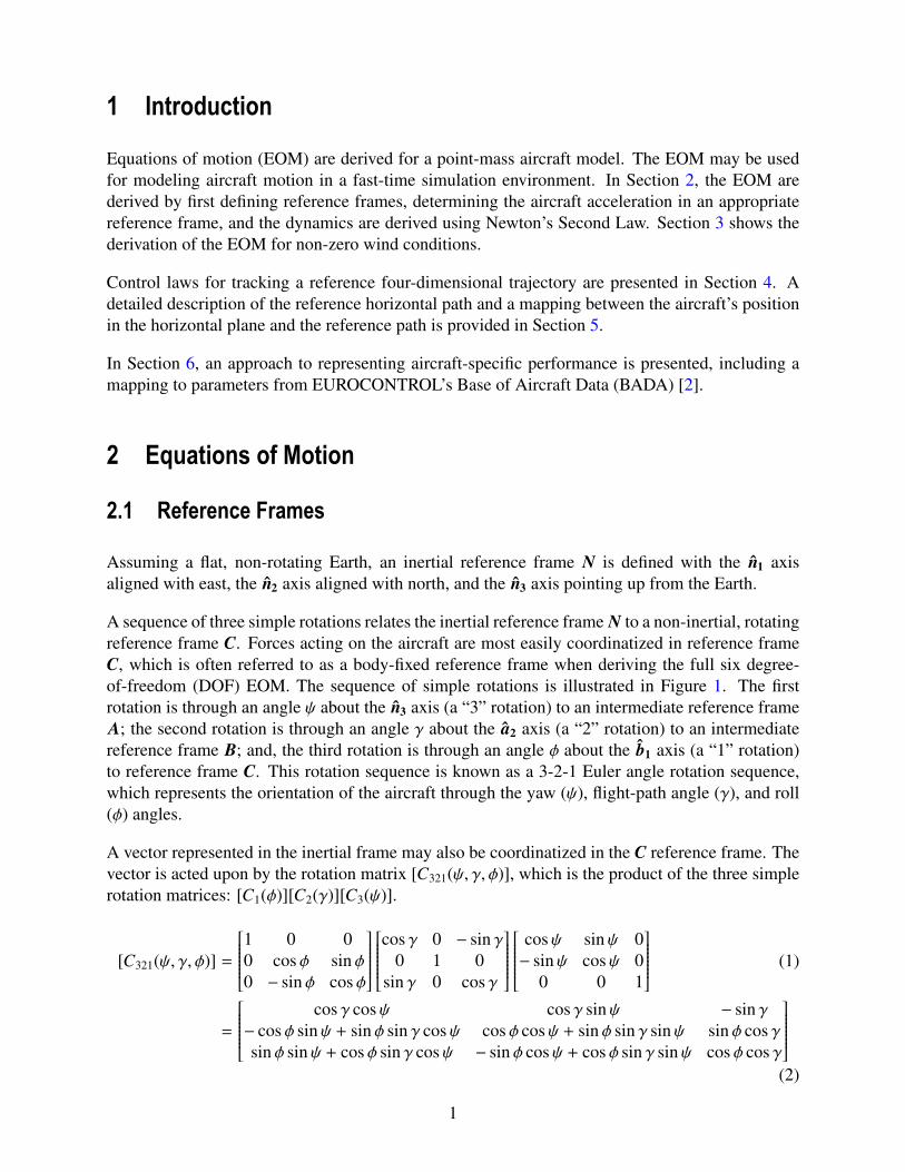
1 Introduction

Equations of motion (EOM) are derived for a point-mass aircraft model. The EOM may be usedfor modeling aircraft motion in a fast-time simulation environment. In Section 2, the EOM arederived by first defining reference frames, determining the aircraft acceleration in an appropriatereference frame, and the dynamics are derived using Newton’s Second Law. Section 3 shows thederivation of the EOM for non-zero wind conditions.

Control laws for tracking a reference four-dimensional trajectory are presented in Section 4. Adetailed description of the reference horizontal path and a mapping between the aircraft’s positionin the horizontal plane and the reference path is provided in Section 5.

In Section 6, an approach to representing aircraft-specific performance is presented, including amapping to parameters from EUROCONTROL’s Base of Aircraft Data (BADA) [2].

2 Equations of Motion

2.1 Reference Frames

Assuming a flat, non-rotating Earth, an inertial reference frame N is defined with the n1 axisaligned with east, the n2 axis aligned with north, and the n3 axis pointing up from the Earth.

A sequence of three simple rotations relates the inertial reference frame N to a non-inertial, rotatingreference frame C. Forces acting on the aircraft are most easily coordinatized in reference frameC, which is often referred to as a body-fixed reference frame when deriving the full six degree-of-freedom (DOF) EOM. The sequence of simple rotations is illustrated in Figure 1. The firstrotation is through an angle ψ about the n3 axis (a “3” rotation) to an intermediate reference frameA; the second rotation is through an angle γ about the a2 axis (a “2” rotation) to an intermediatereference frame B; and, the third rotation is through an angle φ about the b1 axis (a “1” rotation)to reference frame C. This rotation sequence is known as a 3-2-1 Euler angle rotation sequence,which represents the orientation of the aircraft through the yaw (ψ), flight-path angle (γ), and roll(φ) angles.

A vector represented in the inertial frame may also be coordinatized in the C reference frame. Thevector is acted upon by the rotation matrix [C321(ψ, γ, φ)], which is the product of the three simplerotation matrices: [C1(φ)][C2(γ)][C3(ψ)].

[C321(ψ, γ, φ)] =

1 0 00 cos φ sin φ0 − sin φ cos φ

cos γ 0 − sin γ

0 1 0sin γ 0 cos γ

cosψ sinψ 0− sinψ cosψ 0

0 0 1

(1)

=

cos γ cosψ cos γ sinψ − sin γ− cos φ sinψ + sin φ sin γ cosψ cos φ cosψ + sin φ sin γ sinψ sin φ cos γsin φ sinψ + cos φ sin γ cosψ − sin φ cosψ + cos φ sin γ sinψ cos φ cos γ

(2)

1

n1

n2a2

a1

ψ

ψ

a 3

a 1γ

γ

b 1

b 3 c3

φ

φ

b2

b3

c2

Figure 1. Sequence of three simple rotations: 3-2-1 Euler angle orientation sequence.

2.2 Kinematics

The inertial position of the aircraft is given by the following.

P = xn1 + yn2 + hn3 (3)

The inertial velocity can be written in the N and C reference frames.

V = xn1 + yn2 + hn3 = V c1 (4)

Here, V is the aircraft’s true airspeed (TAS), which is equal to the inertial velocity only when thereare no winds.

To derive the EOM using Newton’s Second Law, the inertial acceleration, coordinatized in the Cframe, is determined using transport theorem [1].

Nddt

(V) =Cddt

(V) + ωC/N × V (5)

The angular-velocity vector relating the C frame to the N frame, ωC/N , is given by the addition ofangular velocities. Here, the angular velocities are expressed in the C frame by pre-multiplying bythe appropriate rotation matrices.

ωC/N = ωC/B + ωB/A + ωA/N (6)

= [φ, 0, 0]T + [C1(φ)][0, γ, 0]T + [C1(φ)][C2(γ)][0, 0, ψ]T (7)

ωC/N =(φ − ψ sin γ

)c1 +

(γ cos φ + ψ cos γ sin φ

)c2 +

(−γ sin φ + ψ cos γ cos φ

)c3 (8)

Making the appropriate substitutions into equation (5) yields the following expression for the iner-tial acceleration.

V = V c1 + V(−γ sin φ + ψ cos γ cos φ

)c2 − V

(γ cos φ + ψ cos γ sin φ

)c3 (9)

2

The kinematic equations are determined by projecting V c1 into the inertial frame using the trans-pose of the rotation matrix, [C321(ψ, γ, φ)]T ; x, y, and h are the velocities along the inertial axes,n1, n2, and n3, respectively.x

yh

=

cos γ cosψ − cos φ sinψ + sin φ sin γ cosψ sin φ sinψ + cos φ sin γ cosψcos γ sinψ cos φ cosψ + sin φ sin γ sinψ − sin φ cosψ + cos φ sin γ sinψ− sin γ sin φ cos γ cos φ cos γ

V00

(10)

The inertial velocity of the aircraft can be expressed as shown.

V = V cos γ cosψn1 + V cos γ sinψn2 − V sin γn3 (11)

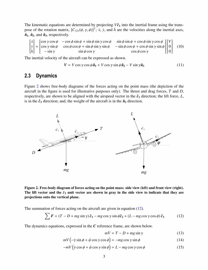
2.3 Dynamics

Figure 2 shows free-body diagrams of the forces acting on the point mass (the depiction of theaircraft in the figure is used for illustrative purposes only). The thrust and drag forces, T and D,respectively, are shown to be aligned with the airspeed vector in the c1 direction; the lift force, L,is in the c3 direction; and, the weight of the aircraft is in the n3 direction.

L

D

T

mg

c 1c 3

− γ

L

mg

c 3

c 2φ

Figure 2. Free-body diagram of forces acting on the point mass: side view (left) and front view (right).The lift vector and the c3 unit vector are shown in gray in the side view to indicate that they areprojections onto the vertical plane.

The summation of forces acting on the aircraft are given in equation (12).∑F = (T − D + mg sin γ) c1 − mg cos γ sin φc2 + (L − mg cos γ cos φ) c3 (12)

The dynamics equations, expressed in the C reference frame, are shown below.

mV = T − D + mg sin γ (13)

mV(−γ sin φ + ψ cos γ cos φ

)= −mg cos γ sin φ (14)

−mV(γ cos φ + ψ cos γ sin φ

)= L − mg cos γ cos φ (15)

3

To decouple equations (14) and (15), equation (14) is multiplied by sin φ and equation (15) ismultiplied by cos φ and the resulting expressions are added to get an equation for γ.

mVγ = −L cos φ + mg cos γ (16)

In a similar manner, equation (14) is multiplied by cos φ and equation (15) is multiplied by sin φand the second expression is subtracted from the first to get an equation for ψ.

mV cos γψ = −L sin φ (17)

The aircraft EOM are the following six first-order ordinary differential equations (ODEs), com-prised of three kinematic and three dynamic equations.

x = V cos γ cosψ (18)y = V cos γ sinψ (19)

h = −V sin γ (20)

V =T − D

m+ g sin γ (21)

γ = −L cos φ

mV+

g cos γV

(22)

ψ = −L sin φ

mV cos γ(23)

3 Equations of Motion with Winds

3.1 Derivation

Suppose there is a constant wind field with wind velocity expressed in the inertial reference frame.

Vw = Vwx n1 + Vwy n2 (24)

The inertial velocity of the aircraft can be expressed as

VC/N = VC/W + VW/N , (25)

where VC/W is the velocity of the aircraft relative to the wind frame W, and VW/N is the windvelocity relative to the inertial frame, which moves with velocity Vw relative to the inertial frame.The inertial velocity is found by adding equations (11) and (24).

V = (V cos γ cosψ + Vwx) n1 +(V cos γ sinψ + Vwy

)n2 − V sin γn3 (26)

Given a constant wind field, the inertial velocity in equation (26) and the dynamics equations(21)-(23) comprise the EOM.

However, given a non-constant wind field, the time derivative of the wind velocity must be consid-ered in the dynamics. The inertial acceleration, expressed in the C frame, has the following form

4

when wind-velocity derivatives are included.

V =[V +

(Vwxcγcψ + Vwycγsψ

)]c1+[

V(−γsφ + ψcγcφ

)+ Vwx (−cφsψ + sφsγcψ) + Vwy (cφcψ + sφsγsψ)

]c2+ (27)[

−V(γcφ + ψcγsφ

)+ Vwx (sφsψ + cφsγcψ) + Vwy (−sφcψ + cφsγsψ)

]c3

Here, s(·) ≡ sin(·) and c(·) ≡ cos(·).

Applying Newton’s Second Law for the inertial acceleration in equation (27) and decoupling theequations for γ and ψ (as described in Section 2.3) results in the following set of equations.

V =T − D

m+ g sin γ − Vwx cos γ cosψ − Vwy cos γ sinψ (28)

γ =−L cos φ + mg cos γ

mV+

1V

(Vwx sin γ cosψ + Vwy sin γ sinψ

)(29)

ψ = −L sin φ

mV cos γ+

1V cos γ

(Vwx sinψ − Vwy cosψ

)(30)

Often wind velocities are provided in a grid format, where the wind speed and direction are givenat a point in the horizontal plane and at an altitude for a given time. Assuming that Vwx and Vwy arefunctions of t, x, y, and h, the time derivative of Vwx and Vwy can be computed by the chain rule.For example:

Vwx(t, x, y, h) =dVwx

dt=∂Vwx

∂t+

(∂Vwx

∂x

) (∂x∂t

)+

(∂Vwx

∂y

) (∂y∂t

)+

(∂Vwx

∂h

) (∂h∂t

)(31)

=∂Vwx

∂t+

(∂Vwx

∂x

)x +

(∂Vwx

∂y

)y +

(∂Vwx

∂h

)h (32)

Additionally, it can be assumed that the wind conditions change slowly with time (∂Vwx/∂t ≈ 0).If the wind gradients in the x and y directions are much less than the wind gradient with respectto altitude (∂Vwx/∂x, ∂Vwx/∂y << ∂Vwx/∂h), the time rate of change of the wind velocity can besimplified to the following.

Vwx(t, x, y, h) =

(∂Vwx

∂h

)h = −

(∂Vwx

∂h

)V sin γ (33)

Substituting equation (33) and a similar expression for the wind derivative in the n2 direction intothe dynamics equations in (28)-(30) results in the following.

V =T − D

m+ g sin γ + V

(∂Vwx

∂h· cosψ +

∂Vwy

∂h· sinψ

)sin γ cos γ (34)

γ =−L cos φ + mg cos γ

mV−

(∂Vwx

∂h· cosψ +

∂Vwy

∂h· sinψ

)sin2 γ (35)

ψ = −L sin φ

mV cos γ−

(∂Vwx

∂h· sinψ −

∂Vwy

∂h· cosψ

)tan γ (36)

Equations (34)-(36) in combination with the kinematic equations for x, y, and h, which are deter-mined from the n1, n2, and n3 components in equation (26), respectively, form the EOM for thepoint-mass aircraft model with non-constant winds.

5

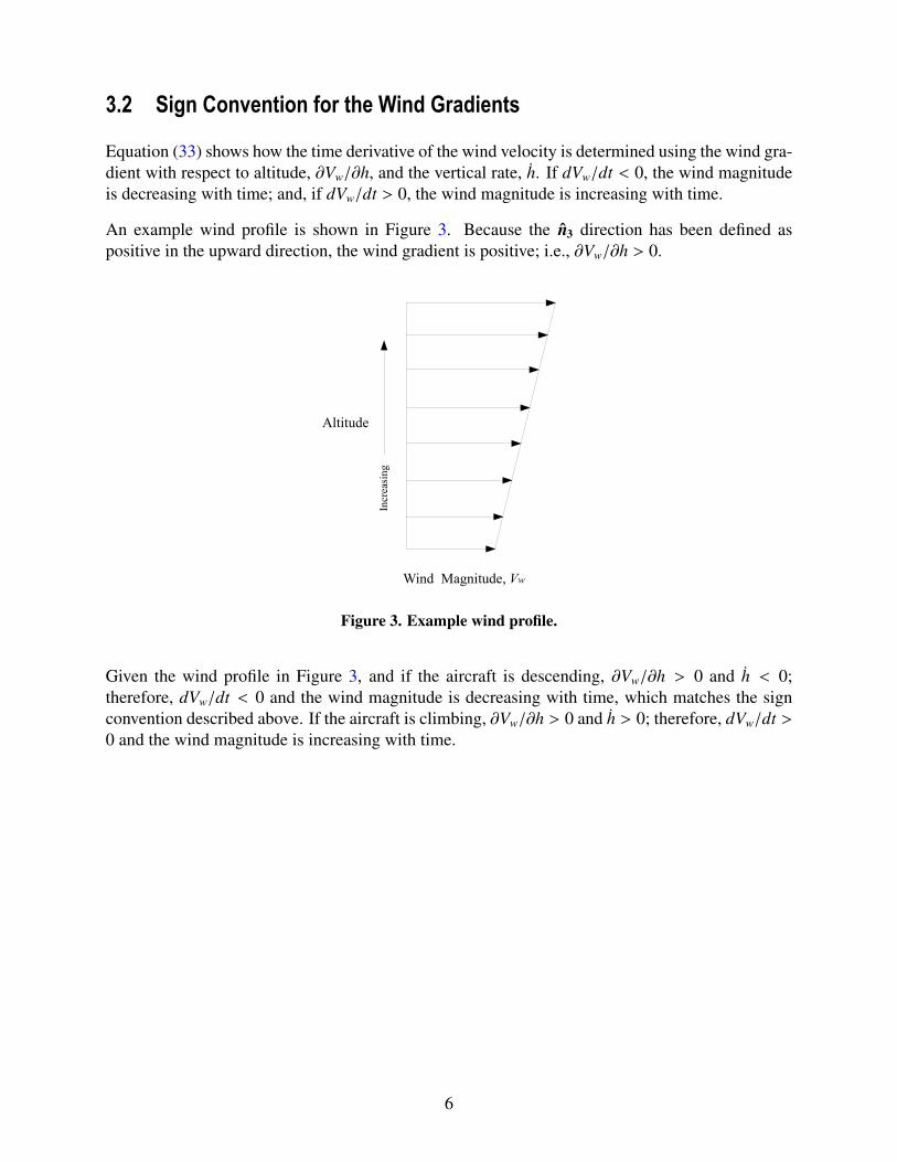
3.2 Sign Convention for the Wind Gradients

Equation (33) shows how the time derivative of the wind velocity is determined using the wind gra-dient with respect to altitude, ∂Vw/∂h, and the vertical rate, h. If dVw/dt < 0, the wind magnitudeis decreasing with time; and, if dVw/dt > 0, the wind magnitude is increasing with time.

An example wind profile is shown in Figure 3. Because the n3 direction has been defined aspositive in the upward direction, the wind gradient is positive; i.e., ∂Vw/∂h > 0.

Altitude

Wind Magnitude, Vw

Incr

easi

ng

Figure 3. Example wind profile.

Given the wind profile in Figure 3, and if the aircraft is descending, ∂Vw/∂h > 0 and h < 0;therefore, dVw/dt < 0 and the wind magnitude is decreasing with time, which matches the signconvention described above. If the aircraft is climbing, ∂Vw/∂h > 0 and h > 0; therefore, dVw/dt >0 and the wind magnitude is increasing with time.

6

4 Guidance Control LawsThe control inputs to the point-mass aircraft model are T , γ, and φ. Equation (29) is replacedwith a first-order differential equation to track a commanded flight-path angle, γc, with gain kγ;wind-gradient effects on the flight-path angle tracking are still included.

γ = kγ (γc − γ) −(∂Vwx

∂h· cosψ +

∂Vwy

∂h· sinψ

)sin2 γ (37)

First-order differential equations for thrust and roll angle also augment the equations of motion tomodel non-instantaneous changes to T and φ, where the gains kT and kφ are chosen to realisticallymodel the aircraft’s response.

T = kT (Tc − T ) (38)φ = kφ (φc − φ) (39)

Here, Tc and φc are the commanded thrust and roll angle, respectively.

The guidance control laws are designed to track a reference horizontal path, a reference calibratedairspeed (CAS), and a reference vertical profile. These reference inputs (and other inputs such asvertical rate) are determined from a pre-calculated four-dimensional trajectory that is generatedby the aircraft’s Flight Management System and is designed for a specified navigation procedure,which may include altitude and speed constraints at waypoints along the procedure.

When the aircraft is in level flight, the airspeed is controlled using thrust. However, there are twospeed-management modes during the descent:

• Speed control using thrust: speed is managed using thrust and the altitude is managed usingpitch (or flight-path angle in the point-mass model described here); and,

• Speed control using pitch: speed is managed by changing the pitch of the aircraft and thealtitude is managed by modulating the thrust.

A speed brake model is also included to increase drag in cases when the aircraft needs to decelerate(in the speed control using thrust mode) or decrease its altitude (in the speed control using pitchmode), but is limited by the current state of the aircraft and/or its control inputs. When the speedbrake is fully deployed, the drag coefficient is increased by 60%. To model the non-instantaneousdeployment of the speed brake, the speed brake deployment fraction, b, is modeled as a first-orderdifferential equation as shown.

b = kspeed brake (bc − b) (40)

Here, kspeed brake prescribes the rate of deployment and bc is the commanded speed brake deploy-ment fraction (e.g., 1.0 indicates full deployment and 0.5 indicates that the speed brake is onlydeployed halfway).

The lateral control law and the control laws for airspeed and altitude for each of the speed-management modes are described in the following subsections. Logic for deploying the speedbrakes is included in the descriptions of the speed-management modes.

7

4.1 Lateral Control

The lateral control law is a function of the heading error, eψ, and the cross-track error, extrk.

The heading error is the error in the commanded heading and the current heading.

eψ = ψc − ψ (41)

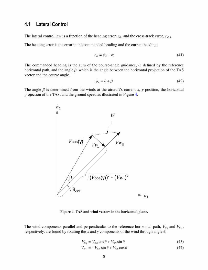
The commanded heading is the sum of the course-angle guidance, θ, defined by the referencehorizontal path, and the angle β, which is the angle between the horizontal projection of the TASvector and the course angle.

ψc = θ + β (42)

The angle β is determined from the winds at the aircraft’s current x, y position, the horizontalprojection of the TAS, and the ground speed as illustrated in Figure 4.

θcrs

β

n

n

1

2

Vcos(γ) Vw ||Vw

W

(Vcos(γ)) - (Vw )2 2

Figure 4. TAS and wind vectors in the horizontal plane.

The wind components parallel and perpendicular to the reference horizontal path, Vw|| and Vw⊥ ,respectively, are found by rotating the x and y components of the wind through angle θ.

Vw|| = Vwx cos θ + Vwy sin θ (43)Vw⊥ = −Vwx sin θ + Vwy cos θ (44)

8

The ground speed, Vgs, and the wind magnitude, W, are calculated as shown.

Vgs =

√(V cos γ)2

− V2w⊥ + Vw|| (45)

W =

√V2

wx + V2wy (46)

The magnitude of β is found using the Law of Cosines.

|β| = cos−1

(V cos γ)2 + V2gs −W2

2V cos γ · Vgs

(47)

The sign of β is opposite to the sign of Vw⊥ .

β = −|β| · sign(Vw⊥

)(48)

The heading error should be limited to [−π, π) to prevent a turn that is greater than 180 degrees.

The cross-track error is the perpendicular distance between the aircraft’s current position and thereference horizontal path. Equations to calculate the cross-track error based on the aircraft’s x, yposition and the reference horizontal path are presented in Section 5.2.1.

The commanded roll angle is computed as a linear function of the heading and cross-track errors.

φc = −kψeψ − kxtrkextrk (49)

4.2 Speed Control Using Thrust

The airspeed control law is a simple proportional control law that determines the desired accel-eration from which the commanded thrust may be computed using dynamic inversion. The com-manded calibrated airspeed, VCAS c , is converted to a commanded TAS, Vc. The desired accelera-tion, Vc, is a function of the error between the current and the commanded TAS.

Vc = kV (Vc − V) (50)

The commanded thrust, Tc, is found by solving equation (34) for T and substituting the desiredacceleration for V .

Tc = mVc + D − mg sin γ − mV(∂Vwx

∂h· cosψ +

∂Vwy

∂h· sinψ

)sin γ cos γ (51)

The commanded thrust is bounded by the maximum and minimum thrust values, Tmax and Tmin,respectively. Section 6 describes how Tmax and Tmin are calculated for a specific aircraft type.

The altitude control law commands a flight-path angle, γc, to manage the aircraft’s altitude relativeto the reference vertical profile defined by the reference altitude, hre f , and the reference verticalrate, hre f .

γc = sin−1

−(hre f + kaltealt

)V

, where ealt = hre f − h (52)

9

If the commanded thrust, Tc, is less than Tmin, the current CAS is checked against the upper CASlimit for the next flaps configuration to determine if the flight crew can deploy the next flaps settingto increase drag.1 The speed brake is deployed if the minimum thrust is commanded for more than15 seconds and if the current TAS is more than 5 kt faster than Vc. The speed brake is deployedfor at least 30 seconds or until the commanded thrust is greater than the minimum thrust (i.e.,Tc > Tmin).

The following algorithm describes the logic for checking the aircraft configuration in the case thatTc < Tmin. The function getConfigForDrag is detailed in Section 6. At the start of the simulation,minThrustCounter is initialized to 0, and the current flaps configuration is initialized based on theaircraft’s current CAS per the function getCon f ig, which is also detailed in Section 6.

Algorithm 1 Configuration for Increased Drag (Speed on Thrust)

if(Tc < Tmin) thenTc = Tmin

newFlapCon f ig = getCon f igForDrag (VCAS , h, hFAF , currentFlapCon f ig)minThrustCounter = minThrustCounter + 1

elseminThrustCounter = 0if(Tc > Tmax)

Tc = Tmax

end ifend if

The use of speed brakes is detailed in the following algorithms: Algorithm 2 is used to determinewhen to deploy speed brakes, and Algorithm 3 is used to determine when to retract speed brakes.

Algorithm 2 Speed Brake Deployment Logic (Speed on Thrust)

if(minThrustCounter > 15 AND (Vc − V) < −5.0 kt) thenif(newFlapCon f ig=={CR,AP,LDG}) then

if(speedBrakeOn== f alse) thenspeedBrakeCounter = 0bc = 0speedBrakeOn = true

elsespeedBrakeCounter = speedBrakeCounter + 1bc = 0.5

end ifelse

speedBrakeCounter = 0bc = 0speedBrakeOn = f alse

end ifend if1The aircraft model is assumed to have four potential flaps configurations: cruise (CR), approach (AP), landing

(LDG), and landing with gear (LDG+GEAR), which are described more fully in Section 6.

10

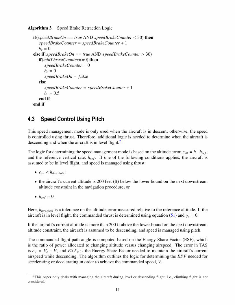
Algorithm 3 Speed Brake Retraction Logic

if(speedBrakeOn == true AND speedBrakeCounter ≤ 30) thenspeedBrakeCounter = speedBrakeCounter + 1bc = 0

else if(speedBrakeOn == true AND speedBrakeCounter > 30)if(minThrustCounter==0) then

speedBrakeCounter = 0bc = 0speedBrakeOn = f alse

elsespeedBrakeCounter = speedBrakeCounter + 1bc = 0.5

end ifend if

4.3 Speed Control Using Pitch

This speed management mode is only used when the aircraft is in descent; otherwise, the speedis controlled using thrust. Therefore, additional logic is needed to determine when the aircraft isdescending and when the aircraft is in level flight.2

The logic for determining the speed management mode is based on the altitude error, ealt = h−hre f ,and the reference vertical rate, hre f . If one of the following conditions applies, the aircraft isassumed to be in level flight, and speed is managed using thrust:

• ealt < hthreshold;

• the aircraft’s current altitude is 200 feet (ft) below the lower bound on the next downstreamaltitude constraint in the navigation procedure; or

• hre f = 0

Here, hthreshold is a tolerance on the altitude error measured relative to the reference altitude. If theaircraft is in level flight, the commanded thrust is determined using equation (51) and γc = 0.

If the aircraft’s current altitude is more than 200 ft above the lower bound on the next downstreamaltitude constraint, the aircraft is assumed to be descending, and speed is managed using pitch.

The commanded flight-path angle is computed based on the Energy Share Factor (ESF), whichis the ratio of power allocated to changing altitude versus changing airspeed. The error in TASis eV = Vc − V , and ES F0 is the Energy Share Factor needed to maintain the aircraft’s currentairspeed while descending. The algorithm outlines the logic for determining the ES F needed foraccelerating or decelerating in order to achieve the commanded speed, Vc.

2This paper only deals with managing the aircraft during level or descending flight; i.e., climbing flight is notconsidered.

11

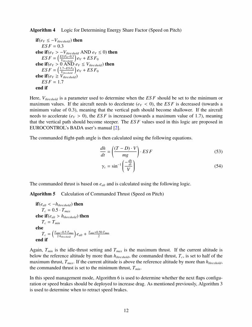
Algorithm 4 Logic for Determining Energy Share Factor (Speed on Pitch)

if(eV ≤ −Vthreshold) thenES F = 0.3

else if(eV > −Vthreshold AND eV ≤ 0) thenES F =

(ES F0−0.3Vthreshold

)eV + ES F0

else if(eV > 0 AND eV ≤ Vthreshold) thenES F =

(1.7−ES F0Vthreshold

)eV + ES F0

else if(eV ≥ Vthreshold)ES F = 1.7

end if

Here, Vthreshold is a parameter used to determine when the ES F should be set to the minimum ormaximum values. If the aircraft needs to decelerate (eV < 0), the ES F is decreased (towards aminimum value of 0.3), meaning that the vertical path should become shallower. If the aircraftneeds to accelerate (eV > 0), the ES F is increased (towards a maximum value of 1.7), meaningthat the vertical path should become steeper. The ES F values used in this logic are proposed inEUROCONTROL’s BADA user’s manual [2].

The commanded flight-path angle is then calculated using the following equations.

dhdt

=

((T − D) · V

mg

)· ES F (53)

γc = sin−1

−dhdt

V

(54)

The commanded thrust is based on ealt and is calculated using the following logic.

Algorithm 5 Calculation of Commanded Thrust (Speed on Pitch)

if(ealt < −hthreshold) thenTc = 0.5 · Tmax

else if(ealt > hthreshold) thenTc = Tmin

elseTc =

(Tmin−0.5·Tmax

2·hthreshold

)ealt + Tmin+0.50·Tmax

2end if

Again, Tmin is the idle-thrust setting and Tmax is the maximum thrust. If the current altitude isbelow the reference altitude by more than hthreshold, the commanded thrust, Tc, is set to half of themaximum thrust, Tmax. If the current altitude is above the reference altitude by more than hthreshold,the commanded thrust is set to the minimum thrust, Tmin.

In this speed management mode, Algorithm 6 is used to determine whether the next flaps configu-ration or speed brakes should be deployed to increase drag. As mentioned previously, Algorithm 3is used to determine when to retract speed brakes.

12

Algorithm 6 Configuration for Increased Drag (Speed on Pitch)

if(Tc == Tmin) thenif(ealt > hthreshold) then

newFlapCon f ig = getCon f igForDrag (VCAS , h, hFAF , currentFlapCon f ig)if(newFlapCon f ig == currentFlapCon f ig AND newFlapCon f ig == {CR, AP, LDG})then

speedBrakeCounter = speedBrakeCounter + 1bc = 0.5speedBrakeOn = true

end ifend ifminThrustCounter = minThrustCounter + 1

elseminThrustCounter = 0

end if

4.4 Control Gains and Parameter Values

The control gains and thresholds used in the guidance control laws are presented in Table 1.

Table 1. Control Gains and Parameter Values

Control Gain ValuekT 0.352 s−1

kφ 0.4 s−1

kspeed brake 0.10 s−1

kψ 3.0kxtrk 5 × 10−4 m−1

kV 0.1136 s−1

kalt 0.20 s−1

hthreshold 500 ftVthreshold 10 kt

13

5 Reference Horizontal PathThe aircraft is controlled to a reference horizontal path, a reference altitude, and a reference CAS,which are determined from a four-dimensional trajectory. The reference altitude and airspeed areprovided as a function of along-path position (or distance-to-go [DTG]); therefore, the referenceinputs are determined using the aircraft’s along-path position.

The reference horizontal path is described in detail in this section, including an algorithm formapping the aircraft’s x, y position to an along-path position.

5.1 Data Format for the Horizontal Path

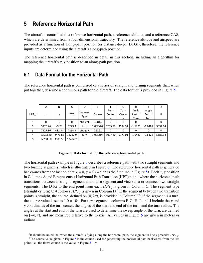
The reference horizontal path is comprised of a series of straight and turning segments that, whenput together, describe a continuous path for the aircraft. The data format is provided in Figure 5.

A B C D E F G H I J

HPT_j x y DTGSegment

TypeCourse

Turn

Center

x

Turn

Center

y

Angle

Start of

Turn

Angle

End of

Turn

R

1 0 0 0 straight 6.2814 0 0 0 0 0

2 5279.26 -9.23 5279.3 turn 1.00E+07 5285.72 3684.91 -1.5725 -1.0487 3694.14

3 7127.86 482.84 7214.3 straight 0.5221 0 0 0 0 0

4 10593.80 2476.82 11212.9 turn 1.00E+07 8007.20 6973.01 -1.0487 -0.6128 5187.14

5 12250.50 3989.59 13474.2 - - - - - - -

Figure 5. Data format for the reference horizontal path.

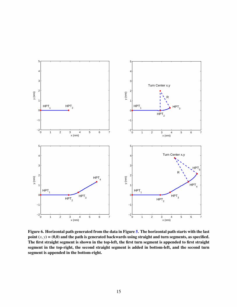
The horizontal path example in Figure 5 describes a reference path with two straight segments andtwo turning segments, which is illustrated in Figure 6. The reference horizontal path is generatedbackwards from the last point at x = 0, y = 0 (which is the first line in Figure 5). Each x, y positionin Columns A and B represents a Horizontal Path Transition (HPT) point, where the horizontal pathtransitions between a straight segment and a turn segment and vice versa or connects two straightsegments. The DTG to the end point from each HPT j is given in Column C. The segment type(straight or turn) that follows HPT j is given in Column D.3 If the segment between two transitionpoints is straight, the course, defined on [0, 2π), is provided in Column E4; if the segment is a turn,the course value is set to 1.0 × 107. For turn segments, columns F, G, H, I, and J include the x andy coordinates of the turn center, the angles of the start and end of the turn, and the turn radius. Theangles at the start and end of the turn are used to determine the sweep angle of the turn, are definedon [−π, π), and are measured relative to the x-axis. All values in Figure 5 are given in meters orradians.

3It should be noted that when the aircraft is flying along the horizontal path, the segment in line j precedes HPT j.4The course value given in Figure 5 is the course used for generating the horizontal path backwards from the last

point; i.e., the flown course is the value in Figure 5 + π.

14

0 1 2 3 4 5 6 7−2

−1

0

1

2

3

4

5

x (nmi)

y (n

mi)

HPT2

HPT1

0 1 2 3 4 5 6 7−2

−1

0

1

2

3

4

5

x (nmi)

y (n

mi)

HPT1

HPT2

HPT3

Turn Center x,y

R

0 1 2 3 4 5 6 7−2

−1

0

1

2

3

4

5

x (nmi)

y (n

mi)

HPT1

HPT2

HPT3

HPT4

0 1 2 3 4 5 6 7−2

−1

0

1

2

3

4

5

x (nmi)

y (n

mi)

HPT1

HPT2

HPT5

HPT4

HPT3

Turn Center x,y

R

Figure 6. Horizontal path generated from the data in Figure 5. The horizontal path starts with the lastpoint (x, y) = (0,0) and the path is generated backwards using straight and turn segments, as specified.The first straight segment is shown in the top-left, the first turn segment is appended to first straightsegment in the top-right, the second straight segment is added in bottom-left, and the second turnsegment is appended in the bottom-right.

15

5.2 Mapping to Along-Path Position

The along-path position of the aircraft is found by orthogonally projecting the aircraft’s x, y posi-tion onto the reference horizontal path. Figure 7 illustrates the high-level process for determiningthe along-path position.

Calculate Distance dj between x,y and

HPTj, j = 1..M

Calculate cross-track error for HPTj with smallest distance dj

no Calculate cross-track error for HPTj (sorted by dj)

yes

index = index(min(dj))

Determine next downstream HPT

Calculate Distance-To-Go to downstream HPT

Along-path Position = –1 x (Distance-To-Go to downstream HPT +

Distance-To-Go from downstream HPT to PTP)

Is cross-track error < 2.5 nmi?

Is cross-track error < 2.5 nmi?

index = j

yes

no

j = j – 1

Figure 7. High-level process for determining the along-path position by projecting the aircraft’s x, yposition onto the reference horizontal path.

The distance between the x, y position and HPT j for j = 1..M is calculated using the Euclideandistance. Starting with the HPT point that results in the smallest distance, d j, the cross-track erroris calculated between the aircraft’s position and the horizontal path.

If the absolute value of the cross-track error is less than 2.5 nmi, then determine the next down-stream HPT. Otherwise, check the cross-track error for the HPT with the next smallest value of d j.Continue checking the cross-track errors until finding an HPT that meets the 2.5-nmi threshold.The DTG and along-path position are then calculated using the next downstream HPT.

The cross-track error and along-path position calculations are detailed below.

16

5.2.1 Cross-track Error Calculation

The cross-track error is calculated by first identifying the whether the aircraft is on a straight or aturn segment. This is done by defining four equal quadrants around HPT j and determining whichquadrant the aircraft’s x, y position falls within. Figure 8 shows a horizontal path defined by HPT j

for j = 1..4, comprised of two straight segments and one turn segment. If j = 2, meaning thatthe aircraft is closest in distance to HPT2, the quadrants are defined using α = course(HPT2) + π.If j = 1 or j = 3, then α = course(HPT1) + π or α = course(HPT3) + π, respectively. The fourquadrants are then defined as follows.

• quadrant 1: [α, α + π/2)

• quadrant 2: [α + π/2, α + π)

• quadrant 3: [α + π, α + 3π/2)

• quadrant 4: [α + 3π/2, α + 2π)

The angle between the aircraft’s position and HPT j is defined on [0, 2π) and is determined as:

θHPT j = atan2(y − y(HPT j), x − x(HPT j)

)(55)

To determine the quadrant where the aircraft is located, θHPT j is checked against the bounds ofeach quadrant. For example, if θHPT j is within quadrant 1, then diff1 = |α − θHPT j | ≤ π/2 ANDdiff2 = |α + π/2 − θHPT j | ≤ π/2. It should be noted the differences in angles must be defined on[−π, π).

The following logic is then applied to determine the next downstream HPT based on the quadrantthat contains the aircraft’s position and the segment type.

Algorithm 7 Logic for Determining Downstream HPT

if[segment(HPT j) == turn AND (quadrant == 1 OR quadrant == 4)] thennextHPT = j − 1

else if[segment(HPT j) == turn AND (quadrant == 2 OR quadrant == 3)] thennextHPT = j

else if[segment(HPT j) == straight AND (quadrant == 1 OR quadrant == 4)] thenif j == 1 then

nextHPT = 1else

nextHPT = j − 1end if

else if[segment(HPT j) == straight AND (quadrant == 2 OR quadrant == 3)] thennextHPT = j

end if

nextHPT is then used to determine whether the aircraft is on a straight or a turn segment: segment(nextHPT).Figure 8 shows three examples of aircraft positions in the horizontal plane: a, b, and c. If the air-craft is located at position a, nextHPT = 1 and the aircraft is assumed to be on a straight segment.

17

HPT1

HPT2

HPT3

1

43

2

1132

4

HPT4

a

b

c

Figure 8. Illustration of quadrants around each HPT.

If the aircraft is located at positions b or c, nextHPT = 2 and the aircraft is assumed to be on aturn segment.

For straight segments, the cross-track error, extrk, is calculated using the following equations.

θ = course(nextHPT), θ : [0, 2π) (56)extrk = − [x − x(nextHPT)] sin θ +

[y − y(nextHPT)

]cos θ (57)

If the aircraft is determined to be on a turn segment, the cross-track error is found using the fol-lowing equations.

R1 =

√(x − xturncenter (nextHPT)

)2+

(y − yturncenter (nextHPT)

)2 (58)

extrk = |R1 − R(nextHPT)| · θdir (59)

Here, θdir is the direction of the turn. If the course angle at the end of the turn is greater than at thestart of the turn, θdir = 1; otherwise, θdir = −1.

18

5.2.2 Along-Path Position Calculation

The DTG to the end point is calculated as a function of the downstream HPT point and the segmenttype (straight or turn).

The DTG is the cumulative path length from the next HPT to the end point, L(nextHPT), plus thedistance from the aircraft’s current position to nextHPT , DTG(nextHPT ).

DTG = L(nextHPT ) + DTG(nextHPT ) (60)

If the aircraft is on a straight segment, the DTG(nextHPT ) is given by the following.

DTG(nextHPT ) = [x − x(nextHPT)] cos θ +[y − y(nextHPT)

]sin θ (61)

If the aircraft is on a turn segment, the following equations are used to find DTG(nextHPT ).

θturn = atan2(y − yturncenter (nextHPT ), x − xturncenter (nextHPT )

)(62)

∆θ = θturnstart − θturn, ∆θ : [−π, π) (63)DTG(nextHPT ) = R · |∆θ| (64)

Figure 9 illustrates the quantities used to calculate the DTG for both a straight and a turn segment.From aircraft position a, the DTG is calculated to the downstream point HPT1. From aircraftposition c on the turn segment, the distance to HPT2 is the arclength of the projection onto thehorizontal path, and the DTG is the sum of that distance and the distance from HPT2 to HPT1.

HPT1

HPT2

HPT3

HPT4

c

d

Dq

DqR

a

Figure 9. Projection of aircraft positions onto horizontal path to determine DTG to end point (HPT1).

It is assumed that the along-path positions are negative and decreasing along the path to zero at thefinal point. Therefore, the DTG is multiplied by −1 to get the along-path position.

19

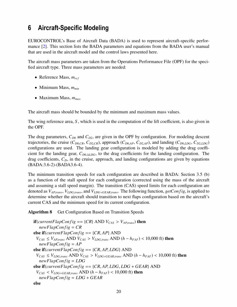
6 Aircraft-Specific ModelingEUROCONTROL’s Base of Aircraft Data (BADA) is used to represent aircraft-specific perfor-mance [2]. This section lists the BADA parameters and equations from the BADA user’s manualthat are used in the aircraft model and the control laws presented here.

The aircraft mass parameters are taken from the Operations Performance File (OPF) for the speci-fied aircraft type. Three mass parameters are needed:

• Reference Mass, mre f

• Minimum Mass, mmin

• Maximum Mass, mmax

The aircraft mass should be bounded by the minimum and maximum mass values.

The wing reference area, S , which is used in the computation of the lift coefficient, is also given inthe OPF.

The drag parameters, CD0 and CD2, are given in the OPF by configuration. For modeling descenttrajectories, the cruise (CD0,CR, CD2,CR), approach (CD0,AP, CD2,AP), and landing (CD0,LDG, CD2,LDG)configurations are used. The landing gear configuration is modeled by adding the drag coeffi-cient for the landing gear, CD0,∆LDG, to the drag coefficients for the landing configuration. Thedrag coefficients, CD, in the cruise, approach, and landing configurations are given by equations(BADA:3.6-2)-(BADA3.6-4).

The minimum transition speeds for each configuration are described in BADA: Section 3.5 (b)as a function of the stall speed for each configuration (corrected using the mass of the aircraftand assuming a stall speed margin). The transition (CAS) speed limits for each configuration aredenoted as VAP,trans, VLDG,trans, and VLDG+GEAR,trans. The following function, getCon f ig, is applied todetermine whether the aircraft should transition to next flaps configuration based on the aircraft’scurrent CAS and the minimum speed for its current configuration.

Algorithm 8 Get Configuration Based on Transition Speeds

if(currentFlapCon f ig == {CR} AND VCAS > VAP,trans) thennewFlapCon f ig = CR

else if(currentFlapCon f ig == {CR, AP} ANDVCAS ≤ VAP,trans AND VCAS > VLDG,trans AND (h − hFAF) < 10,000 ft) then

newFlapCon f ig = APelse if(currentFlapCon f ig == {CR, AP, LDG} AND

VCAS ≤ VLDG,trans AND VCAS > VLDG+GEAR,trans AND (h − hFAF) < 10,000 ft) thennewFlapCon f ig = LDG

else if(currentFlapCon f ig == {CR, AP, LDG, LDG + GEAR} ANDVCAS < VLDG+GEAR,trans AND (h − hFAF) < 10,000 ft) then

newFlapCon f ig = LDG + GEARelse

20

newFlapCon f ig = currentFlapCon f igend if

Because the commanded CAS, VCAS , must be limited to the upper CAS speed limit for a givenconfiguration, the upper speed limits for each configuration (VAP,max, VLDG,max, and VLDG+GEAR,max)will also be provided for each aircraft type. The function getCon f igForDrag, described below, isused to determine whether the next flaps configuration can be deployed to increase drag. Inputs tothe function are the aircraft’s current CAS, VCAS , the aircraft’s current altitude, h, and the currentconfiguration, currentFlapCon f ig.

Algorithm 9 Get Configuration for Increased Drag

if(currentFlapCon f ig == CR AND VCAS < VAP,max AND (h − hFAF) < 10,000 ft) thennewFlapCon f ig = AP

else if(currentFlapCon f ig == AP AND VCAS < VLDG,max AND (h − hFAF) < 10,000 ft) thennewFlapCon f ig = LDG

else if(currentFlapCon f ig == LDG AND VCAS < VLDG+GEAR,max AND (h − hFAF) < 10,000 ft)then

newFlapCon f ig = LDG + GEARelse

newFlapCon f ig = currentFlapCon f igend if

The drag force, D, is calculated as a function of air density, wing reference area, and the TAS usingequation (BADA:3.6-5). The lift force is calculated similarly.

L =CL · ρ · V2 · S

2

The thrust parameters are also given in the OPF and are as follows:

• CTc,1

• CTc,2

• CTc,3

• CTdes,high

• CTdes,low

• CTdes,app

• CTdes,ld

• Hp,des

The maximum engine thrust, Tmax, is modeled using equations (BADA:3.7-1) and (BADA:3.7-8), assuming no temperature deviations from the standard atmospheric model. The minimum

21

thrust, Tmin, is modeled as a function of altitude and configuration using equations (BADA:3.7-9)-(BADA:3.7-12).

The maximum operating calibrated airspeed (CAS) and Mach are given in the OPF as VMO andMMO, respectively.

The standard atmospheric model is given in Section BADA:3.1; conversions between CAS andTAS are described in equations (BADA:3.1-23) and (BADA:3.1-24).

22

7 References[1] J. E. Hurtado, Kinematic and Kinetic Principles. Hurtado - Lulu.com, 2007.

[2] “User manual for the base of aircraft data (BADA) revision 3.11,” Tech. Rep., May 2013,Eurocontrol Experimental Center Technical/Scientific Report No. 13/04/16-01.

23

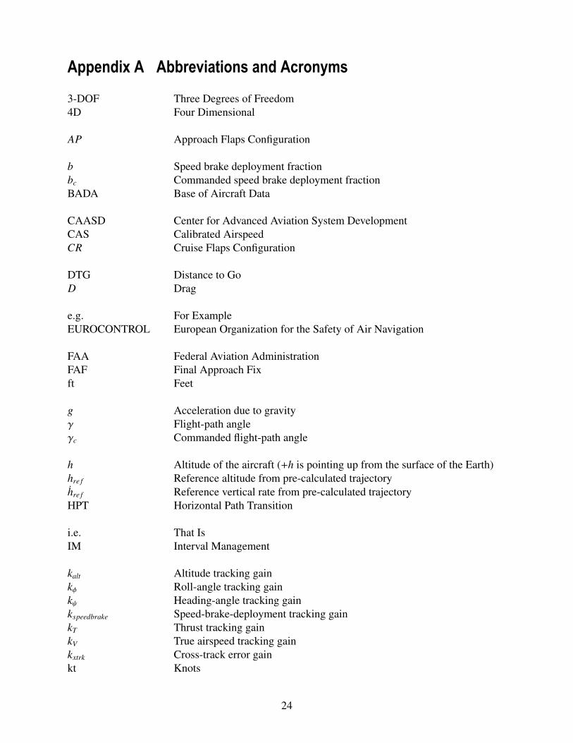
Appendix A Abbreviations and Acronyms3-DOF Three Degrees of Freedom4D Four Dimensional

AP Approach Flaps Configuration

b Speed brake deployment fractionbc Commanded speed brake deployment fractionBADA Base of Aircraft Data

CAASD Center for Advanced Aviation System DevelopmentCAS Calibrated AirspeedCR Cruise Flaps Configuration

DTG Distance to GoD Drag

e.g. For ExampleEUROCONTROL European Organization for the Safety of Air Navigation

FAA Federal Aviation AdministrationFAF Final Approach Fixft Feet

g Acceleration due to gravityγ Flight-path angleγc Commanded flight-path angle

h Altitude of the aircraft (+h is pointing up from the surface of the Earth)hre f Reference altitude from pre-calculated trajectoryhre f Reference vertical rate from pre-calculated trajectoryHPT Horizontal Path Transition

i.e. That IsIM Interval Management

kalt Altitude tracking gainkφ Roll-angle tracking gainkψ Heading-angle tracking gainkspeedbrake Speed-brake-deployment tracking gainkT Thrust tracking gainkV True airspeed tracking gainkxtrk Cross-track error gainkt Knots

24

L Lift forceLDG Landing Flaps ConfigurationLDG + GEAR Landing Flaps Configuration plus Landing Gear

m Aircraft mass

nmi Nautical Miles

φ Roll angleφc Commanded roll angleψ Heading angleψc Commanded heading angle

sec Seconds

T Thrust forceTc Commanded thrust forceθ Course-angle guidance from the reference horizontal pathθnextHPT Angle between the x, y position of the aircraft and the next downstream

Horizontal Path Transitionθturn Angle between the x, y position of the aircraft and the center of the turn for

the next downstream Horizontal Path TransitionTOD Top of Descent

V True airspeed of the aircraftV Time rate of change of the TASV Inertial velocity vectorVAP,max Maximum CAS in the Approach Flaps ConfigurationVAP,trans Minimum Speed to transition from Cruise Flaps Configuration to the Ap-

proach Flaps ConfigurationVc Commanded TASVCAS c Commanded calibrated airspeedVLDG,max Maximum CAS in the Landing Flaps ConfigurationVLDG,trans Minimum Speed to transition from Approach Flaps Configuration to the

Landing Flaps ConfigurationVLDG+GEAR,max Maximum CAS in the Landing Flaps + Gear ConfigurationVLDG+GEAR,trans Minimum Speed to transition from Landing Flaps Configuration to the

Landing Flaps + Gear ConfigurationVw Wind velocity vectorVw|| Wind speed aligned with aircraft’s courseVw⊥ Wind speed perpendicular to aircraft’s courseVwx Wind speed in the x directionVwy Wind speed in the y direction

x Position of the aircraft in the x direction in the horizontal plane (+x direc-tion is aligned with East)

25

y Position of the aircraft in the y direction in the horizontal plane (+y direc-tion is aligned with North)

26

Disclaimer

The contents of this material reflect the views of the author and/or the Director of the Center forAdvanced Aviation System Development (CAASD), and do not necessarily reflect the views of theFederal Aviation Administration (FAA) or the Department of Transportation (DOT). Neither theFAA nor the DOT makes any warranty or guarantee, or promise, expressed or implied, concerningthe content or accuracy of the views expressed herein.

This is the copyright work of The MITRE Corporation and was produced for the U.S. Governmentunder Contract Number DTFAWA-10-C-00080 and is subject to Federal Aviation AdministrationAcquisition Management System Clause 3.5-13, Rights in Data-General, Alt. III and Alt. IV (Oct.1996). No other use other than that granted to the U.S. Government, or to those acting on behalfof the U.S. Government, under that Clause is authorized without the express written permission ofThe MITRE Corporation. For further information, please contact The MITRE Corporation, Con-tract Office, 7515 Colshire Drive, McLean, VA 22102 (703) 983-6000.

c©2015 The MITRE Corporation. The Government retains a nonexclusive, royalty-free right topublish or reproduce this document, or to allow others to do so, for “Government Purposes Only.”

27