1

Deploying Sensor Networks withGuaranteed Fault Tolerance

Jonathan L. Bredin,∗ Erik D. Demaine,† MohammadTaghi Hajiaghayi,‡ Daniela Rus†

Abstract—We consider the problem of deploying or repairinga sensor network to guarantee a specified level of multi-pathconnectivity (k-connectivity) between all nodes. Such a guaranteesimultaneously provides fault tolerance against node failures andhigh overall network capacity (by the max-flow min-cut theorem).We design and analyze the first algorithms that place an almost-minimum number of additional sensors to augment an existingnetwork into a k-connected network, for any desired parameter k.Our algorithms have provable guarantees on the quality of thesolution. Specifically, we prove that the number of additionalsensors is within a constant factor of the absolute minimum,for any fixed k. We have implemented greedy and distributedversions of this algorithm, and demonstrate in simulation thatthey produce high-quality placements for the additional sensors.

I. INTRODUCTION

SENSOR-NETWORK applications owe much of their pop-ularity to broad and rapid deployment, frequently into

hazardous environments. We use a robotic helicopter to deploysensors to monitor outdoor environments and provide networkconnectivity for emergency response scenarios [1], [2]. Suchrapid deployment, especially under extreme circumstances,exposes sensors to additional chance of failure and placementerrors. Sensors may not be placed in exactly their desiredlocations because of wind or inaccurate localization. Sensorsmay fail from impact of deployment, fire or extreme heat,animal or vehicular accidents, malicious activity, or simplyfrom extended use. These failures may occur upon deploymentor over time after deployment: extensive operation may drainsome of the nodes’ power, and external factors may phys-ically damage part of the nodes. Additionally, hazards maychange devices’ positions over time, possibly disconnectingthe network. If any of these initial deployment errors, sensorfailures, or change in sensor positions cause the network tobe disconnected or lack other desired properties, we need todeploy additional sensors to repair the network.

In an example application, a network of cameras monitorsthe safety of a building compound. Each sensor does localimage analysis to detect events such as motion within its

A preliminary version of this paper appeared at MOBIHOC 2005.∗Department of Mathematics and Computer Science, Colorado College, 14

East Cache la Poudre Street, Colorado Springs, CO 80903, USA, jbredin@coloradocollege.edu†Computer Science and Artificial Intelligence Laboratory, Massachusetts

Institute of Technology, 32 Vassar Street, Cambridge, MA 02139, USA,edemaine,rus@csail.mit.edu‡ AT&T Labs — Research, 180 Park Ave., Florham Park, NJ 07932, USA.

hajiagha@mit.edu. This work was done while the author was at MIT andMicrosoft Research.

Manuscript received March 8, 2007; revised May 28, 2009.

field of view. Upon such events, sensors send images toa base station for more complex analysis such as tracking.This application relies on the network’s ability to supporta given amount of information flow. The application alsoillustrates that not all the nodes in the network require thesame amount of communication. For example, the nodes alongthe trajectory of the tracked object will transmit more imagesand thus use more power to communicate. This means thattheir communication ability will be diminished and they maybecome depleted of power. In such a case, the network willhave to be extended with new nodes to sustain the desiredinformation flow.

Given the dynamic environment, it is desirable to haveprocedures to establish network properties, such as connected-ness, in the event that multiple devices fail. We are interestedin developing an algorithm that can run regularly in thebackground, to suggest repairs to a deployment mechanismonce connectivity properties disappear. Upon the detectionof network failures, our algorithm computes the locationswhere an approximately minimum number of additional nodesneed to be deployed in the network using a ground or flyingrobot. This results in a goal-directed approach for automatedmaintenance and repair of a network which optimizes the useof the powerful mobile node (e.g., the robot helicopter) taskedto do this operation by deploying additional sensors.

More specifically, to support both fault tolerance and capac-ity, we focus on the vertex-connectivity of the network. Thek-connectivity property has been studied extensively before inthe context of wireless networks; see [3], [4] and their manycitations. In the worst case, a k-connected network requiresk node failures to disconnect the network. Additionally, k-connectivity ensures a high overall transport capacity of thenetwork, by the max-flow min-cut theorem.

Given a desired value of k, we present and analyze a genericalgorithm that determines how to establish k-connectivity byplacing additional sensors geographically between existingpairs of sensors. Here, in order for the problem to be well-defined, we assume that the sensors’ locations are known (ei-ther directly by the sensors via GPS, or by an external agent’ssurvey and measurement) and that sensor communication isdefined by the unit-disk graph model, so that we can predicthow the communication graph changes as we add sensors.Solving this problem with a minimum number of additionalsensors is NP-hard [5]. Our approach is to transform the net-work repair problem to one of selecting the minimum-weightk-vertex connected subgraph of the complete graph underlyingthe sensor network and then applying existing graph-theoreticapproximation methods. Our proposed algorithm provides a

2

bound on the solution quality that is within a constant factorof the optimal solution, for any fixed k. (More precisely, theapproximation ratio is O(k4α), where α = O(lg k) is the bestapproximation ratio for a related problem [6], [7].)

Due to limited communication or computational resourcesavailable to nodes, our proposed provable approximation al-gorithm for optimal k-connectivity repair may be difficult toimplement on a physical sensor network. This limitation maynot be significant because the algorithm can usually be runoccasionally and in the background, so there is little need fora “real time” algorithm. Nonetheless, our characterization ofthe problem complexity shows how to further approximatethe problem. We develop alternative methods for determininga low-cost k-connected graph that are simpler, faster, and ableto run in the distributed sensor network. The modularity ofour base algorithm allows us to trade computational speed forsolution accuracy. In an experimental study, we implement insimulation the use of greedy and distributed algorithms andshow that, in practice, the solution quality produced by thesefast methods is not far from optimal.

Attaining k-connectivity has recently been studied in thecontext of power assignment, where instead of adding sensorsthe goal is to assign the sensors’ communication power toensure k-connectivity and minimize overall power consump-tion. This problem is also NP-hard. Ramanathan and Rosales-Hain [8] consider the special case of 2-connectivity andprovide a centralized spanning-tree heuristic for minimizingthe maximum transmit power in this case. Bahramgiri et al. [3]generalize the cone-based local heuristic of Wattenhofer etal. [9], [10] in order to solve the general k-connectivity setting.However, both of these works are heuristics and do not haveprovable bounds on the solution cost [11]. Lloyd et al. [12]present an 8-approximation algorithm for 2-connectivity, butthey do not consider general k-connectivity. Hajiaghayi etal. [11] present a constant-factor approximation algorithm fork-connectivity for any fixed k. Recently, different sets ofauthors (see e.g. [13], [14], [15], [16]) used the notion ofk-connectivity and the results of [3], [11] to deal with thefault-tolerance issues for static and dynamic settings.

Our problem has been considered before only in the specialcase k = 1, where the problem has applications in VLSIdesign and evolutionary/phylogenetic tree constructions incomputational biology. See [17] for a description of theseand other applications, and [18] for early work on the theoryof general graphs. The best approximation algorithm to ourknowledge for our context of unit-disk graphs is a 5/2-approximation algorithm by Du et al. [19], again only for thecase k = 1.

We proceed by introducing some definitions, notation, andmodels we will use for our algorithm. Section III presentsan algorithm that takes the subgraph-repair problem as amodular black box to establish k-vertex connectivity in anetwork by adding new nodes geographically between exist-ing ones. Whereas the algorithm is natural, the analysis inSection IV providing an approximation bound is complicated.We present in Section V practical distributed modifications toour algorithm and implement one on computationally limitedplatforms upon which the ideal approximation algorithms

would be difficult to implement. Section VI supports theheuristics through experiments whose simulations compare theperformance of our simplified algorithms with our algorithmusing optimal subgraph repair. The experiments show that ourmethods are superior to deployment according to additionalrandom sampling. Finally, we conclude in Section VII withdiscussion of improvements to our algorithm relying on tighteranalysis to derive a polynomial-time approximation scheme.

The conference version of this paper inspired or has beenused in several followup papers, e.g., [20], [21], [22], [4], [23],[24], [25], [26], [27], [28], [29], [30], [31], [32], [33], [34],[35], [36], [37], [38], [39], [40]; see also [41], [42], [43].

II. PRELIMINARIES AND MODELS

In this paper we consider static symmetric multi-hop ad-hocwireless networks with omni-directional fixed-power transmit-ters that typically arise in the context of sensor networks. Thismodel is considered by Blough et al. [44], Calinescu et al. [45],Kirousis et al. [46], and others in their works on connectivity.The model has many practical consequences; for example,many existing routing protocols can easily be accommodatedby this model, in particular because links are bidirectional.Furthermore, many of the restrictions imposed by this modelcan be relaxed at the cost of additional communication. Wesummarize the main features of the model here.

An ad-hoc wireless network consists of a set of mobiledevices (e.g., sensors) equipped with radio transceivers. Ingeneral, each radio transmitter can be assigned a powersetting and an orientation that define the reception area ofits transmissions. We assume that all transmitters have acommon, fixed maximum power setting, and refer to that as thecommunication radius. We also assume that the transceiversare omni-directional in the sense that they transmit and receivein all directions equally. Both of these assumptions are satisfiedby most wireless networks. We also assume that the signalpropagation is uniform in all directions, so in particular thereare no radio-opaque obstacles.

We make the further assumptions that our networks arestatic and that all communication links are bidirectional orsymmetric. In a static network, the devices are stationary. Ifa device moves, the topology of the network can change inways out of our control. In the symmetric link model, if adevice u can receive transmissions from a device v, then ualso has enough maximum power to transit to device v. Inpractice, most wireless networks experience problems fromasymmetries, but the symmetric restriction simplifies routingprotocols. We assume that the nodes in our networks tunedown their effective ranges to the lowest common range.

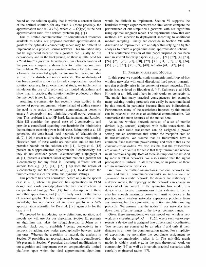
Given these assumptions, we can model our wireless net-work as a unit-disk graph, G = (V,E), where each vertex rep-resents a device and is assigned two-dimensional coordinates.Two vertices are connected by an edge if and only if theirdistance is at most the communication radius. For simplicityof exposition, we normalize the coordinate assignment sothat the communication radius is 1. The unit-disk graphmodel is widely used, e.g., in the past theoretical work onconnectivity [19] as well as in certain practical scenarios withcarefully engineered radios [47].

3

a

Fig. 1. An example unit-disk graph.

In this paper we suppose that the network is multi-hop,meaning that the mobile devices cooperate to route eachothers’ messages. Thus we are interested in multi-node com-munication paths between the source and destination of amessage. In anticipation of node failures resulting e.g. frompower failure or power depletion of a mobile node, we are alsointerested in finding multiple disjoint communication pathsbetween any source/destination pair.

In this paper we consider the following problem, given asensor network represented as a unit-disk graph, we wishto compute and deploy the minimum number of additionaldevices to ensure that the resulting unit-disk graph satisfiesthe fault-tolerance constraint called vertex k-connectivity. Agraph is vertex k-connected if there are at least k vertex-disjoint paths connecting every pair of vertices, or equivalently,the graph remains connected when any set of at most k − 1vertices is removed. Hence our goal is to make the networkresilient to k node failures. In the problem we consider, we aregiven such a plane unit-disk graph and our goal is to deploythe minimum number of additional sensors to ensure one oftwo fault-tolerance constraints on the resulting unit-disk graph:either there should be k paths in the new network betweenevery pair of original sensors, or there should be k paths in thenew network between every pair of (old or new) sensors. Wecall the first constraint partial k-connectivity and the secondconstraint full k-connectivity.

Fig. 1 shows an example unit-disk graph that is not 3-connected. The largest component of the graph is 1-connectedas it can be separated with the removal of the vertex marked a,for example. The graph in Fig. 2 shows the same graph withadditional vertices to establish 3-connectivity among verticesfrom the original graph.

Our problem has been considered before only in the specialcase k = 1, where the problem has also found application inVLSI design and evolutionary/phylogenetic tree constructionsin computational biology. See [17] for a description of theseand other applications. The problem is NP-hard even for k =1 [5]. The best approximation algorithm to our knowledge isa 5/2-approximation algorithm by Du et al. [19], again onlyfor the case k = 1.

An important related problem is, given a weighted completegraph K and a number k ≥ 1, to find minimum-weight

Fig. 2. The example unit-disk graph from Fig. 1 with added vertices,marked with dashed circles, to establish 3-connectivity among the original(solid) vertices. The new vertices lie closely enough to each other to ensure3-connectedness for the entire graph. We omit drawing edges between theadded vertices for clarity.

k-vertex-connected subgraph of K. This problem can beviewed as analogous to our problem of k-fault tolerance butfor wired networks. Frank and Tardos [48] and Khuller andRaghavachari [49] were among the first authors who workedon this problem. The problem is NP-hard, and there are bynow several polynomial-time approximation algorithms withguaranteed performance ratios. An α-approximation algorithmis a polynomial-time algorithm whose solution cost is atmost α times the optimal solution cost. Kortsarz and Nu-tov [6] developed a k-approximation algorithm. At the heartof this algorithm is a combinatorial algorithm of Gabow [50]whose running time is O(k2|V |2|E|) (an improvement toan algorithm of Frank and Tardos [48]). They also developbetter approximation algorithms for small k, specifically, anapproximation ratio of d(k + 1)/2e for k ≤ 7. Cheriyan etal. [7] improved the Θ(k) approximation ratio with an O(lg k)-approximation algorithm, provided that the number of verticesin the graph is at least 6k2. This algorithm is based on aniterative rounding method and the ellipsoid algorithm appliedto a linear-programming relaxation of exponential size, andhence is not very practical.

Our algorithms will use as a subroutine any one of theseapproximation algorithms for minimum-weight k-connectedsubgraph. We suppose that the subroutine we use has anapproximation ratio of α, and state our own approximationratio in terms of α. This generality allows us to choosean algorithm according to practicality, or to chose a futureimprovement to the state-of-the-art for this problem, andunderstand the impact on the final approximation ratio. Notethat a better approximation algorithm, with performance ratio2 + (k − 1)/n [6], is known if the graph weights satisfythe triangle inequality, but the weighted complete graphs weconsider do not satisfy this property. Algorithm 1 presents theformal operation.

III. ALGORITHM FOR CONNECTIVITYREPAIR

In this section we describe our algorithm for minimizingthe number of additional sensors to guarantee k-connectivity.

4

The algorithm is relatively simple, building on approximationalgorithms for minimum-weight k-vertex-connected subgraph.This modular design allows us to use several candidate algo-rithms for finding k-connected subgraphs and achieve a rangeof trade-offs between quality and performance. In particular,we can use a constant-factor approximation algorithm for k-connected subgraphs and obtain a constant-factor approxima-tion algorithm for k-connectivity repair, for any fixed k. Theanalysis of this algorithm is complicated because we need toprove that the simplicity of the algorithm does not preventit from finding more intricate, better solutions; this topic isaddressed in the next section.

Algorithm 1 K-CONNECTIVITY-REPAIR

1: input: k, set V of vertices and their coordinates2: if n ≥ k then3: E ← (v, w) | v, w ∈ V, v 6= w4: K ← (V,E)5: ω ← new V × V array6: for vertices v, w ∈ V do7: ω[v, w]← d‖v − w‖e − 18: end for9: call K-CONNECTED-SUBGRAPH (k,K, ω)

to compute α-approximate minimum-weightk-connected spanning subgraph S of (K,ω)

10: for edge (v, w) ∈ E(S) do11: for i = 1, 2, . . . , ω[v, w] do12: t← i/(ω[v, w] + 1)13: place k sensors at position (1− t) · v + t · w14: place k − 1 sensors at position v15: place k − 1 sensors at position w16: end for17: end for18: else19: call K-CONNECTIVITY-REPAIR (1, V )20: N ← newly placed sensors21: for x ∈ V ∪N do22: place k − 1 sensors at position x23: end for24: end if

The algorithm divides into two cases. Our descriptionconcentrates on the main case that the number n of originalsensors is at least the desired connectivity k. The second casethat n < k is simpler and we consider it later.

First we compute a weighted complete graph K on the sameset of vertices as the given graph G. The weight on an edgev, w is one less than the ceiling of the Euclidean distancebetween the two points v and w: ω(v, w) = d‖v − w‖e − 1.This weight is zero if v and w are already connected by anedge in the unit-disk graph G, and otherwise it is the numberof additional sensors required to connect v and w by a straightpath.

Second we run an α-approximation algorithm to find anapproximately minimum-weight k-vertex-connected subgraphof this weighted complete graph K. See Section II for a sum-mary of known theoretical approximation algorithms for thisproblem; see Section V for more practical implementations,

Fig. 3. An illustration of the approximation algorithm’s performancein establishing full 3-connectivity. Solid vertices exist in the input at theperipheral and establish the heavy edges for zero cost. The algorithm choosesto add the thinner edges and places additional sensors, marked with dashedcircles, along the new edges. The optimal repair adds only the shaded vertex.We omit the optimal solution’s edges to avoid clutter.

including a greedy approach and a fast distributed algorithm.Note that our constructed graph K likely does not satisfy thetriangle inequality: if G is connected, then there is a zero-weight path between every pair v, w of vertices, so the triangleinequality would require that all edges v, w have weight 0,which is rarely the case in K. Therefore we can only useapproximation algorithms for general graphs.

Third we translate the chosen edges in the k-vertex-con-nected subgraph of K into a placement of new sensors. Thisstep depends on the desired fault-tolerance constraint. Forpartial k-connectivity, we simply place ω sensors along theline segment connecting the endpoints of each edge of weightω, spaced a unit distance apart. For full k-connectivity, weplace ω clusters of k collocated sensors along the line segmentconnecting the endpoints of each edge of weight ω, spacingthe clusters a unit distance apart. (Of course, in practice, theseclusters can be spread out in a small neighborhood of a pointinstead of all being placed at the same point, at only a smalladditional cost.) In addition, for each edge of weight ω > 0,we place k−1 additional sensors at each endpoint of the edge.

In the case that n < k, the graph K has fewer than k verticesand therefore has no k-connected subgraph. We run thealgorithm for k = 1 to compute an approximately minimumnumber of additional sensors that connect the sensors. Thenwe replicate each original and additional sensor k times byadding k − 1 more copies.

Fig. 3 demonstrates an example of how the approximationalgorithm establishes 3-connectivity to the network formedby the six peripheral vertices. The dark edges have nocost as the original graph already supports them. The K-CONNECTED-SUBGRAPH routine chooses the light edges toestablish 3-connectivity and the approximation places newvertices, marked with dashed circles, along the chosen edges.The optimal solution places a single point, drawn as gray, inthe graph center.

5

IV. ANALYSIS

The main difficulty in the analysis of our algorithm’sperformance ratio is that the Steiner points—i.e., additionalpoints other beyond the input points—can be placed in in-finitely many possible locations. In particular, there may besome locations to place a Steiner point that simultaneouslyinterconnect several pairs of original points. Our algorithmdoes not search for such “hub locations”, nor will it noticethat it found one if it happens to use one. Another, more subtleproblem along the same lines is that it is not always optimalto connect pairs of original points by straight sequences ofSteiner points. Rather, it may be beneficial to connect severaloriginal points by straight lines to common Steiner points. Thisissue is precisely what makes Euclidean Steiner tree NP-hard,in contrast to minimum spanning tree. A third challenge is thatour objective is to (approximately) minimize the number ofadded sensors, not the total number of sensors. In particular, ifthe graph is already k-connected, any approximation algorithmmust not add any sensors, because otherwise the ratio tothe optimal cost of 0 would be infinite. Thus we need toexploit the existing connectivity among the original sensors,because we cannot afford to pay for it again. This moredifficult objective prevents us from using structures whose costdepends on the number of original sensors. (Otherwise wecould repeat a minimum spanning tree on the original sensorsk times, which would be a trivial O(k) approximation on thetotal number of sensors.) These issues prevent us from usingstandard approximation algorithms and analysis based on e.g.minimum spanning trees.

Again we first consider the main case that n ≥ k.Lemma 1: For any set of original and Steiner sensors, there

is a subgraph G′ of the induced unit-disk graph G such that(1) for each edge of G′ incident to at least one Steiner sensor,we can assign it to one of its Steiner endpoints such that eachSteiner sensor is assigned at most 6k edges, and (2) for anyset S of less than k vertices, two vertices are connected inG− S if and only if they are connected in G′ − S.

Proof: We construct G′ by considering the Steiner sensorsin an arbitrary order, and showing by induction that it sufficesto connect each Steiner sensor to at most 6k original sensorsand/or Steiner sensors that come earlier in the order. Lets1, s2, . . . , sm denote the Steiner sensors, ordered arbitrarily.For each 0 ≤ i ≤ m, let Gi denote the graph on all originalsensors and just the first i Steiner sensors s1, s2, . . . , si.Thus Gm = G. We will define a subgraph G′i of Gi for each0 ≤ i ≤ m, such that G′i satisfies the two properties of thelemma with respect to Gi (i.e., substituting Gi and G′i for Gand G′). Thus G′m will serve as the desired G′.

In the base case, G′0 = G0 consists of just the originalsensors, and the desired properties hold trivially: the firstproperty because there are no Steiner sensors, and the secondproperty because G′0 = G0. For the induction step, suppose wehave already constructed G′i−1 and we wish to construct G′i.Each Gi differs from the previous Gi−1 only in that it includesan additional vertex si and some incident edges, and we willconstruct G′i similarly to differ from G′i−1 only around si.Thus for G′i to satisfy the first property we need only that the

degree of si in G′i is at most 6k; then we can assign all ofthese edges to si. We divide the neighbors of si in Gi intosix groups by dividing the unit disk centered at si into sixequal pie wedges of angle 60. (The neighbors of si in Gi areprecisely those sensors in the unit disk centered at si.) Thenwe select k arbitrary neighbors from each of the six groups(or we select the entire group if it has size less than k), andmake those 6k or fewer vertices the neighbors of si in G′i.Certainly si has degree at most 6k in G′i, so the first propertyholds. The key property of this construction is that all verticesin the same group are connected by edges in Gi, because eachpie wedge has diameter 1.

Finally we must show that G′i satisfies the second propertythat, for any set S of less than k vertices, two vertices areconnected in Gi − S if and only if they are connected inG′i−S. Consider some set S of less than k vertices. BecauseG′i is a subgraph of Gi, we need to show only that two verticesv and w connected in Gi − S are also connected in G′i − S.(Thus, in particular, the vertices v and w under considerationare not in S.) If S contains si, then G′i − S = G′i−1 − S andGi−S = Gi−1−S, so by the induction hypothesis on G′i−1 vand w are connected in G′i−1−S = G′i−S. Now we considerthe case that S does not contain si. If v and w are connectedby a path in Gi − S that does not visit si, then that path alsoexists in Gi−1−S, so by induction the vertices are connectedin G′i−1−S and thus in the supergraph G′i−S. (In particular,if S contains si, then this case applies.) Otherwise, we knowthat any path connecting v and w in Gi − S visits si, andthus in particular any such path visits a vertex in the unit diskcentered at si immediately before and after si the path visitsother vertices in the unit disk centered at si.

Let v′ be the first vertex along a path connecting v and win Gi−S that is inside the unit disk centered at si, and let w′

be the last vertex along the same path that is inside the unitdisk centered at si. (Note that v′ might be v, and w′ mightbe w.) Because v and v′ are connected by a path that does notvisit si, by the previous case they are connected in G′i−1−S,and similarly w and w′ are connected in G′i−1−S. We cannothave v′ and w′ in the same pie wedge of the unit disk, becausethen they would be connected via an edge in Gi−1 and thusconnected in Gi−1−S and by induction connected in G′i−1−S,so there would have been a path connecting v and w that doesnot use si.

Now we argue that v′ and si are connected in G′i − S; bya symmetric argument w′ and si are connected in G′i − S,and thus v and w are connected in G′i − S. If v′ = si

(which happens precisely when v = si), then they are triviallyconnected. Otherwise, v′ is in one of the six pie wedgessurrounding si. If there are at most k vertices in the piewedge containing v′, then si has edges to all of them in G′i,and thus in particular there is an edge between si and v′.Otherwise, among the k neighbors of si in G′i in the pie wedgecontaining v′, at least one neighbor v′′ must be in G′i − Sbecause S has size less than k. Because v′ and v′′ are in thesame pie wedge, they are connected by an edge in Gi−1 soby induction connected in G′i−1. Adding the edge between v′′

and si to this path, we find that v′ and si are connected in G′i.Therefore v and w are connected in G′i.

6

This lemma shows that G and the constructed subgraph G′

are essentially the same in terms of connectivity. The next lem-mas show how to remove Steiner points from G′ again withoutlosing any connectivity. We consider separately each “Steinercomponent” defined as follows. The Steiner component rootedat a Steiner sensor s is formed by growing a set of vertices andedges in G′ starting with s and stopping after we reach anyoriginal sensors. The Steiner component includes the edgesconnecting pairs of sensors in the component provided atleast one of the endpoints is a Steiner sensor. (Equivalently, aSteiner component is a connected component of the inducedsubgraph of G′ on the Steiner sensors, together with the edgesconnecting these Steiner sensors to original sensors and theseoriginal sensors.)

Lemma 2: If G′ has at least k original vertices and is vertexk-connected, then the number of original vertices in eachSteiner component is at least k.

Proof: The set of original vertices of a Steiner componentforms a cut in G′ unless that Steiner component is all of G′.In either case we must have at least k original vertices in theSteiner component.

Every Steiner component C has a spanning tree T (C) inwhich the original sensors are leaves of T (C).

Lemma 3: The number of edges in an Eulerian tour of thespanning tree T (C) of a Steiner component C in G′ is at most12k times the number of Steiner sensors in C.

Proof: The number of edges in the Eulerian tour is exactlytwice the number of edges of T (C). Each of these edges can beassigned to one of the Steiner sensors in C, and by Lemma 1,the number of assignments is at most 6k times the numberof Steiner sensors in C. Therefore the number of edges inthe Eulerian tour is at most 12k times the number of Steinersensors in C.

For any integer n ≥ 3 and any positive integer k ≤ n, theHarary graph1 Hk,n is the k-connected graph on n verticesv1, v2, . . . , vn where each vi is connected via an edge tothe preceding dk/2e vertices vi−1, vi−2, . . . , vi−dk/2e and thesucceeding dk/2e vertices vi+1, vi+2, . . . , vi+dk/2e.

We consider the following procedure for replacement of aSteiner component C. First we remove the Steiner sensorsin C. Second we take an Eulerian tour of the spanningtree T (C). Third we construct a Harary graph Hk,m on them original sensors in C ordered by the order in which theEulerian tour visits these leaves of T (C). (By Lemma 2,m ≥ k, so the Harary graph exists.) We view the edges of thisgraph as edges in the weighted complete graph K, and addthese edges to our graph wherever they do not already exist,2 and translate each edge of weight w into a sequence of wsensors equally spaced along the line segment connecting theendpoints. The resulting graph is no longer a unit disk graph:some edges come from the original unit-distance constraint,and others edges come from K. Once we replace all Steinercomponents in G′, we obtain a subgraph of K with no Steiner

1In fact, Harary graphs are normally defined differently when k is odd. Weround up to the Harary graph for the next even value of k in order to obtainthe desired approximation bound in this paper.

2We avoid the addition of multiple edges, but in fact single edges andmultiple edges are equivalent for our purposes of vertex k-connectivity.

sensors.Lemma 4: The total weight of edges of K that replace a

Steiner component C is at most 3k3 + 12(k2 + k) times thenumber of Steiner sensors in C.

Proof: Each edge in the Harary graph connects twooriginal sensors that are within distance at most dk/2e inthe order defined by the Eulerian tour. We charge the weightof this edge to the path of the Eulerian tour that connectsthese two original sensors. The weight of the edge is at mostthe number of edges in the path of the Eulerian tour becausethe edge in K represents a shortcutting of the path taken bythe Eulerian tour. We distribute the charge on the path of theEulerian tour to the subpaths connecting consecutive originalsensors in the Eulerian tour. Each subpath is charged at mostdk/2e2 times, one for each edge of the Harary graph thatspans that subpath. By Lemma 3, the number of edges inthe Eulerian tour is at most 12k times the number of Steinersensors in C. Therefore the total weight of the replacementis at most 12kdk/2e2 ≤ 12k(k/2 + 1)2 = 3k3 + 12(k2 + k)times the number of Steiner sensors in C.

Lemma 5: If G′ is vertex k-connected, then replacement ofall Steiner components in G′ results in a vertex k-connectedsubgraph of K.

Proof: We claim that replacement of a Steiner componentpreserves vertex k-connectivity. Let C1, C2, . . . , Cr denote theSteiner components in G′. For each 0 ≤ i ≤ r, let G′i denoteG′ after replacement of the first i Steiner components. ThusG′0 = G′ is k-connected.

Assume by induction that G′i−1 is k-connected. Considerany set S of less than k vertices in G′i whose removaldisconnects two vertices v and w in G′i−S. By the inductionhypothesis, there is a path connecting v and w in G′i−1 − S.Let v′ and w′ be the first and last vertex along that path thatbelong to Steiner component Ci. Thus v′ and w′ are bothoriginal vertices and therefore also present in G′i. Also, v andv′ are connected by the same subpath in G′i − S, as are wand w′. Because the replacement Harary graph is k-connected,removal of S cannot disconnect it, so v′ and w′ are connectedin the Harary graph and thus in G′i − S. Therefore v and ware connected in G′i − S. The result follows by induction.

Theorem 6: In the case n ≥ k, the algorithm is apolynomial-time O(k4α)-approximation on the minimumnumber of added sensors to attain vertex k-connectivity ofthe entire unit-disk graph.

Proof: Consider the optimal set of added sensors thatresults in a vertex k-connected unit-disk graph G. We constructG′ as in Lemma 1, and then perform a replacement ofeach Steiner component. By Lemmas 1 and 5, the resultingsubgraph of K is vertex k-connected. By Lemma 4, the totalweight of the subgraph of K is at most 3k3 +12(k2 +k) timesthe number of Steiner sensors in G. The minimum-weight k-connected subgraph of K can have only smaller weight, so isalso at most 3k3 + 12(k2 + k) times the number of Steinersensors in G. Our algorithm finds an α-approximation to theminimum-weight k-connected subgraph, and then for everyedge of weight w ≥ 1, adds kw+2k−2 < 3kw sensors. (Thisreplication guarantees vertex k-connectivity of the entire graphbecause the removal of less than k vertices cannot disconnect

7

the subgraph of K, nor can it disconnect the sensors thatconstitute an edge of K.) Therefore the number of sensorsadded by the algorithm is less than (9k4α + 36(k3 + k2)α)times the optimal number of added sensors used in G.

In the second case that n < k, the replication guaranteesvertex k-connectivity of the entire graph because the removalof less than k vertices still leaves at least one copy of theoriginal spanning tree which is connected. We apply the k = 1analysis to show that the number of added sensors for 1-connectivity is O(1) times the optimal. The optimal numberof added sensors for 1-connectivity is certainly a lower boundon the optimal number of added sensors for k-connectivity.The replication of these sensors costs an additional factor of k.The replication of the original sensors uses k(k−1) additionalsensors, which can be charged to the optimal number of addedsensors for k-connectivity, which is at least 1 because theoriginal graph cannot be k-connected. Therefore we obtainan approximation ratio of at most k2 +O(k).

Corollary 7: For any fixed k ≥ 1, our algorithm is an O(1)-approximation on the minimum number of added sensors toattain vertex k-connectivity of the entire unit-disk graph.

The analysis bounds the number of vertices used to establishk-connectivity in the network through considering only pointslying on edges in the complete weighted graph representingthe network. Thus it leads us to simpler algorithms to achievek-connectivity that do not have to consider Steiner points. Wediscuss such an algorithm next.

V. PRACTICAL IMPLEMENTATIONS

In this section we present practical implementations ofthe k-connectivity repair algorithm analyzed in the previoussection. All the algorithms that we consider are based on theK-CONNECTIVITY-REPAIR outline given in Algorithm 1, butthey use different subroutines for K-CONNECTED-SUBGRAPH(line 9). The guaranteed α-approximation algorithms fork-connected subgraphs [6], [7] are based upon solving linearprograms, and implementation may be difficult on compu-tationally and communication-constrained sensor networknodes. Furthermore, because those algorithms are designed tooptimize worst-case behavior, it is unclear how they compareto other algorithms on average-case instances. We implementsimple greedy and distributed algorithms for K-CONNECTED-SUBGRAPH, and show that the resulting approximation factorsin practice are much smaller than the worst-case bounds.

Our two practical algorithms are both based upon greedyapproaches that choose inexpensive repairs. While the straight-forward greedy approach is conceptually simple, it is difficultto implement in a distributed environment. To address suchdifficulty, we present and implement a distributed algorithm,similar in spirit to Garcia-Molina’s invitation leader-electionalgorithm [51], where network nodes elect leaders to makedecisions how to merge k-connected subnetworks.

A. Greedy Approach

Algorithm 2 illustrates a greedy solution to K-CONNECTED-SUBGRAPH. The algorithm consists of two phases. We beginwith an empty subgraph of the specified graph G. In the first

phase, the algorithm repeatedly adds edges (v, w) from thegraph G in increasing order by weight ω(v, w). The first phaseends once the subgraph is k-connected. In the second phase,the algorithm repeatedly attempts to remove edges (v, w) fromthe subgraph, in decreasing order by weight ω(v, w), butputting the edge back if it was necessary for k-connectivity.Experimentally, this pruning stage can remove 58–85% of theadded edges. The resulting subgraph is therefore a k-connectedsubgraph of G, and we expect that the weight of the chosenedges is reasonably small.

Algorithm 2 Greedy K-CONNECTED-SUBGRAPH

1: input: k, G = (V,E), ω2: G′ ← (V, ∅)3: E′ ← (v, w) | v, w ∈ V 4: for (v, w) ∈ E′ in increasing order of ω[v, w] do5: E(G′)← E(G) ∪ (v, w)6: if G′ is k-connected then7: break8: end if9: end for

10: for (v, w) ∈ E(G′) in decreasing order of ω[v, w] do11: G′′ ← (V,E(G′) \ (v, w))12: if G′′ is k-connected then13: G′ ← G′′

14: end if15: end for16: return G′

This greedy algorithm produces the same subgraph as thefollowing less-efficient algorithm: start from the completegraph G as the subgraph, and repeatedly remove edges (v, w)that do not destroy k-connectivity, in decreasing order byweight ω(v, w). For k = 1, this algorithm (and hence theoriginal greedy algorithm) finds the minimum spanning tree;it is essentially dual to Prim’s algorithm. Thus the greedyalgorithm generalizes a minimum-spanning-tree constructionto k ≥ 1, so we expect that it does well.

The greedy algorithm, however, can have arbitrarily poorperformance, as depicted in Figure 4 when the graph forms along narrow U-shaped chain to be repaired to 2-connectivity.The greedy algorithm chooses to reinforce the existing linksby placing new nodes on top of existing ones. The optimalrepair places the two gray nodes to create a loop. Becausethe chain can be arbitrarily long, but still require only a fixednumber of nodes to repair, the ratio of the worst-case greedycost to optimal is unbounded.

On the other hand, for the Steiner version where you onlyhave to k-connect designated vertices, the algorithm can beΩ(n) away from optimal. Consider, for example, two verticesx and y that are connected by two paths, one path with n− 1edges of weight 0 and one edge of weight 1+ ε, and the otherpath with n edges of weight 1. The greedy algorithm for k = 1removes the weight-(1+ε) edge and destroys the path of totalweight 1 + ε, leaving the path of total weight n, for a ratioarbitrarily close to n.

8

Fig. 4. An example of poor performance by the greedy algorithm to establish2-connectivity. The greedy algorithm places the dashed nodes at the sameposition as the existing nodes, whereas the optimal repair places the graynodes to construct a circuit.

B. Distributed Implementation

Algorithm 2 repeatedly tests for k-connectivity—a timeconsuming operation.3 The algorithm also requires globalknowledge of the candidate edges.

To address both problems, we distribute a locally greedyalgorithm that grows and merges k-connected components.The distributed approach relies on a synchronous messagepassing only in that all messages are either delivered or lostforever within a fixed time limit. Each component elects aleader to compute the cost of joining neighboring compo-nents. Two disjoint k-connected components form a larger k-connected component if bridged with k vertex-disjoint edges.Members of a k-connected component report the cost ofjoining some number of the closest other components. Theleader chooses k vertex-disjoint paths used to merge with eachcomponent. The assignment can quickly be computed withan auction-based assignment implementation [52], or usingmore-easily implemented heuristics. Each leader then proposesmerging with its lowest-cost counterpart. A propositionedleader accepts the first offer that matches its lowest computedcost.

When components are smaller then k nodes, leaders mergecomponents by greedily creating k-cliques.

The distributed algorithm relaxes the need for synchroniza-tion, complete centralized knowledge of node distances, andk-connectivity testing. Each node, however, still requires anupper bound of the distance to each other node, obtained eitherby localization [53] or through bounding the distance throughinspecting a routing table. Additionally, the algorithm has nopruning stage similar to the second stage of Algorithm 2, sowe expect it to generate heavier subgraphs.

1) Merging Subnetworks: We now show how the mergingof subnetworks produces a k-connected networks.

Lemma 8: For (n ≤ k), the k-connected graph Gk and then-clique Kn form a k-connected supergraph when bridged sothat every vertex in Kn has k − n + 1 new neighbors in Gand no two vertices in Kn share neighbors in Gk.

Proof: We prove Lemma 8 by contradiction. Suppose thata graph, G, is constructed in the manner of the lemma such

3The runtime improves if the connectivity test first checks that the minimumdegree for each node is at least k. Noting that the minimum degree for eachnode must match or exceed k, and knowing such failure eliminates the needfor many k-connectivity tests.

that it not k-connected, so that its vertices can be partitionedinto non-empty sets A,B and C so that C serves as a cut setseparating the vertices in A and B.claim: A∩ V (Gk) = ∅ or B ∩ V (Gk) = ∅.The claim followsfrom noting that if both A and B contain elements of V (Gk),then Gk could not have been k-connected.

Without loss of generality, let B ∩ V (Gk) = ∅. Thus A ∩V (Kn) 6= ∅, because A is not empty.claim: k < |N (B)|. The claim follows from the expansionthat each v ∈ A, N (v) = k and for each u, v ∈A, N (v)/N (u) 6= ∅.

Thus |C| > k and we arrive at a contradiction that G mustbe k-connected.

Corollary 9: Given a k-connected graph Gk, the super-graph G constructed by adding one additional vertex con-nected to k distinct vertices in Gk is also k-connected.

Corollary 9 is sometimes referred to as the ExpansionLemma.

Corollary 10: The supergraph constructed from two dis-joint k-connected graphs bridged with k vertex-disjoint edgesis k-connected.

2) Protocol: Leader nodes alternate between two modes:invitation and listening. In the invitation mode, a leaderrequests from its followers bridges to other subnetworks, andissues a merge invitation to other leaders. An invitation willonly be accepted if the recipient is in listening mode and theinvitation includes the recipient’s current group size. If theinvitation is accepted the recipient relinquishes leadership andbroadcasts for every group member, the member’s new leader.Through a gossip network, a leader can determine whether itsinvitation has been accepted, or timeout if it hears no suchchange in the gossip network.

If J is the expected time for a node issuing requests to find apartner, δ the time spent waiting for requests, ∆ the time timespent waiting for a replies to a request, and p the probabilitythat a single message is delivered, then an upper-bound for Jcan be expressed as the recurrence

J =δ

∆ + δp∆ +

(1− pδ

∆ + δ

)(∆ + δ + J),

which simplifies to

J =(∆ + δ)2

pδ− δ.

If ∆ is fixed, J is minimized when dJ/dδ to zero, leaving theoptimal latent period to be

δ =∆√

1− p.

A gossip protocol informs the network of group membershipand group size. Only leader nodes may insert new gossip intothe network which uses a logical timestamp associated witheach subject to achieve consistency. A node receiving gossipabout a subject compares the message timestamp with thetimestamp for the subject. If the received timestamp is greaterthan the local one, the node updates its local gossip knowledgeand broadcasts the gossip to its neighbors. If the receivedtimestamp is less than the local one, the node broadcasts its

9

own gossip to the rest of the network. Each node periodicallybroadcasts its own state to ensure that changes are eventuallyrecorded.

3) Message Complexity: We next bound the number ofmessages the algorithm requires to terminate.

Theorem 11: The distributed repair algorithm requiresO(n2) point-to-point messages and O(n2) broadcast messagesto repair a graph to k-connectivity.

Proof: The algorithm proceeds in rounds where eachleader requests to merge with another leader. During eachround, the algorithm merges at least two subnetworks, so thealgorithm terminates after at most n− 1 rounds.

We first count the messages sent to leaders by followersand the merge proposals sent between leaders. Each roundrequires that a leader node send one message to its preferredpartner, and each follower to send to its leader a constantnumber of messages representing links to bridge to anothersubnetwork. No node sends more than a constant number ofmessages either as a leader or follower, hence no node sendsmore than O(n) messages, and the algorithm requires O(n2)messages to terminate.

After each merge operation, the leader must inform therest of the network of its erstwhile followers new groupmembership. A node may change its membership no morethan n − 1 times, thus there are O(n2) broadcast messagesrequired to repair a network to k-connectivity.

VI. EXPERIMENTAL RESULTS

We implement in simulation both the centralized greedy-repair and the distributed solutions from the previous sectionto compare their performance with a sampling-based and theoptimal subgraph repair solutions. The sampling-based algo-rithm scatters new vertices uniformly through the environmentuntil the original nodes are k-connected, similar to the startingpoint of [54], except that we do not require k-connectivity tothe additional nodes. For small graphs, we compare the repairsof each of the three previous algorithms against the optimalplacement, restricted by Algorithm 1, that we compute throughcombinatorial branch-and-bound search using Algorithm 2 asan initial bound.

We test each algorithm on uniformly generated and gridgraphs that have had some portion removed to destroy 3-connectivity. The first graph structures we consider have nodesplaced on a two-dimensional rectangular grid evenly spacedone unit apart. With the exceptions of the corners, these graphsare 3-connected. The second class of graphs are generatedthrough a Las-Vegas method. The vertices are uniformlyplaced inside a fixed-size rectangular area until the resultinggraph is k-connected.

The generated graphs are damaged by one of two meth-ods, uniform selection and geographic selection. The uniformselection method takes size parameters p and n. Verticesare uniformly selected and removed from a graph originallycontaining n vertices until there are fewer than pn vertices re-maining and the graph is no longer 3-connected. The selectionprocess models network failures representing decay over time.

The geographic selection process selects a graph’s twomost-distant nodes, s and t. It repeatedly removes the node

1

10

0 0.1 0.2 0.3 0.4 0.5 0.6 0.7 0.8

repa

ir co

st /

optim

al

% removed

4x4 grid, k=3

randomdistributed

greedy

Fig. 5. The cost, relative to optimal, to repair 4×4 uniformly damaged gridgraphs to 3-connectivity. The figure plots mean repair cost of groups of tenexperiments with error bars denoting the observed (biased) standard deviation.

located mid-way along the shortest remaining s-t path. Wetest our algorithms on augmented graphs that have had onlyenough nodes removed so that k-connectivity does not hold,as well as on graphs that the process completely disconnected.The resulting graphs model networks with geographicallydependent failures.

We measure the number of vertices required to repaira damaged graph to k-connectivity, forgetting the verticesremoved from the original graph. For these experiments, weonly guarantee that the original vertices are k-connected, notthe additional ones. Multiplying the cost by k (for replication)provides an upper bound on the cost of repairs guaranteeingthat the additional vertices are also k-connected. Empirically,however, additional vertices almost always lie closely enoughto k-connected without extra duplication.

Fig. 5 plots the mean number of vertices added to uniformlydamaged graphs to re-establish 3-connectivity to 4×4 gridsfor the greedy, distributed, and randomized implementations.Each of the plotted values are normalized first by the numberof vertices in the damaged graph and then by the optimal costto repair the graph. The greedy algorithm frequently finds theoptimal repair for graphs with more than 30% of their verticesremoved.

It is difficult to measure the optimal cost of larger graphs,but we observe that the repair costs for uniformly damaged10 × 10 grid graphs plotted in Fig. 6 scale similarly to thecosts of 4× 4 before normalization by the optimal.

Figs. 7 and 8 plot results for the same experiments ondenser, uniformly generated graphs. For comparison to opti-mal, we are able only to look at uniformly distributed graphsin a 3 × 3 area, sustaining at most 35% node removal. Theoriginal graphs have on average 48 nodes, but some haveas many as twice that. In repairing these graphs, it appearsthat costs relative to optimal for three repair algorithms areindependent to the portion removed. Table I shows for eachalgorithm the mean cost relative to optimal and χ2 scores withfive degrees-of-freedom. The χ2 goodness-of-fit measure sumsthe squared error of the predicted performance, inferred fromthe mean across the experiments using the same algorithm,

10

0

5

10

15

20

25

30

35

40

45

0 0.2 0.4 0.6 0.8 1

repa

ir co

st /

vert

ex r

emai

n

% removed

10x10 grid, k=3

randomdistributed

greedy

Fig. 6. The cost, relative to the number of vertices remaining, to repairuniformly damaged 10×10 grid graphs to 3-connectivity. The figure plotsmean repair cost of groups of ten experiments with error bars denoting theobserved (biased) standard deviation.

0

0.2

0.4

0.6

0.8

1

1.2

0.05 0.1 0.15 0.2 0.25 0.3 0.35 0.4

repa

ir co

st/v

erte

x re

mai

n

% removed

3x3 uniform, k=3

randomdistributed

greedyoptimal

Fig. 7. The cost of re-establishing 3-connectivity to uniformly damagedgraphs that were originally uniformly generated in a 3×3 area. We plot themean repair cost per remaining vertex and (biased) standard deviation forgroups of 36 experiments.

and the observed performance. The low χ2 scores give uslittle reason to question that algorithm performance, relativeto optimal, is independent to the portion removed. We also plotexperiments on 7×7 uniformly generated graphs that average250 vertices in Fig. 8. Again the repair costs increase similarlyin both of the two scales. Fig. 9 demonstrates the cost to re-establish 3-connectivity to graphs suffering removal of half oftheir vertices as a function of the size of the network afterremoving nodes. Empirically, the cost decreases with the sizeof the network, shown by the plotted regression lines fittingthe logarithm of the cost as a linear function of the networksize.

The performance of the greedy repair algorithm is surprisingand requires some explanation. Fig. 10 shows an exampleof a uniformly generated 3-connected graph. Nodes A, B,and C are removed and the greedy repair algorithm takes theresulting graph as input. The algorithm adds node Z. Node Ais superfluous to preserving connectivity in the original graph;it resides at the graph’s fringe. Because it resides in a denselypopulated region, node B is redundant. Thus, these two node

0

2

4

6

8

10

12

14

0 0.2 0.4 0.6 0.8 1

repa

ir co

st /

vert

ex r

emai

n

% removed

7x7 uniform, k=3

randomdistributed

greedy

Fig. 8. The cost of re-establishing 3-connectivity to uniformly damagedgraphs that were originally uniformly generated in a 7×7 area. We plot themean repair cost relative to optimal and (biased) standard deviation for groupsof ten experiments.

algorithm mean repair cost / optimal χ2 (5 dof)random 5.3 1.35distributed 2.3 0.96greedy 1.5 0.18

TABLE ITHE COST RELATIVE TO OPTIMAL FOR EACH ALGORITHM AND THE χ2

GOODNESS-OF-FIT SCORES WITH FIVE DEGREES OF FREEDOM INDICATINGTHE SUM OF SQUARED DIFFERENCES OF THE SAMPLE MEANS AND THE

GRAND MEAN.

removals require no attention for repair. The greedy algorithmreplaces node C with Z, re-establishing 3-connectivity.

Because many of the vertices uniformly selected to be

0 500 1000 1500 2000

0.0

0.5

1.0

1.5

2.0

network size

repa

ir co

st

50% removed, k=3

0 500 1000 1500 2000

0.0

0.5

1.0

1.5

2.0

0 500 1000 1500 2000

0.0

0.5

1.0

1.5

2.0

0 500 1000 1500 2000

0.0

0.5

1.0

1.5

2.0

randomdistributedgreedy

Fig. 9. The proportion of additional nodes required to restore 3-connectivityto previously 3-connected networks that have had 50% of their nodes removed.We also plot the best-fit regression for ln(cost) = β0 + β1size to illustratethe trend.

11

redundantZ

B

A

fringe

added

C

Fig. 10. A typical graph-repair example. The destruction process removesnodes A, B, and C. The greedy repair algorithm adds node Z.

Fig. 11. An example of complete disconnection, represented by the largerdashed region, and substantial vertex removal, denoted by the dashed circle.

removed from the input graphs did not contribute to thegraph’s k-connectedness, we also test the repair algorithms ongeographically damaged graphs. To better ensure that removedvertices contribute to connectivity, we uniformly generate 3-connected 10×10 unit-disk graphs, select the two most-distantvertices s and t, and remove a vertex in the middle of somenumber the shortest s-t paths. Fig. 11 shows an example 3-connected 10×10 unit-disk graph with two groups of verticesmarked for removal. The smaller, circular grouping denotesa substantial disconnection that will affect k-connectivity,whereas removing the larger group completely disconnects thegraph.

Table II shows the repair costs of removing enough ver-tices to completely disconnect s-t pairs and removing onlyenough edges to destroy k-connectivity. The table shows theincrease in the number of vertices required to re-establish 3-connectivity, relative to the optimal repair cost. As the greedyand distributed algorithms can better localize the area to be

greedy dist randomµ σ µ σ µ σ

complete 1.35 0.72 1.59 0.76 3.94 3.27substantial 2.13 1.68 2.14 2.77 7.65 9.36

TABLE IITHE REPAIR COST RELATIVE TO OPTIMAL OF REPAIRING UNIFORMLY

UNIFORMLY GENERATED 3-CONNECTED 3×3 UNIT-DISK GRAPHS. THETABLE REPORTS THE MEAN AND OBSERVED STANDARD DEVIATION FOR

TEN TRIALS. THE “COMPLETE” ENTRY REPRESENTS GRAPHS THAT WERECOMPLETELY DISCONNECTED, WHEREAS THE “SUBSTANTIAL” ENTRYSHOWS THE REPAIR COST OF REMOVING ONLY ENOUGH VERTICES TO

REMOVE k-CONNECTIVITY FROM THE GRAPH.

repaired, they perform about 3 times better than the randomrepair algorithm.

VII. CONCLUSION

It would be interesting to extend our guaranteed worst-case approximation algorithms to the case of partial k-connectivity, where there should be k vertex-disjoint pathsbetween every pair of original sensors, but not necessarilybetween pairs involving added sensors. This weaker goalis natural if only the original sensors serve a useful pur-pose (e.g., carrying information), and the added sensors onlyserve for additional connectivity between them. We attackthe weaker problem in the experiments, but usually the newpoints are k-connected anyway—not too surprising given thatthere exist density thresholds that probabilistically guaranteek-connectivity. Even minimum degree k is enough to probablygive k-connectivity [55]. But what about the worst case? Avariation of our approach may lead to efficient approximationalgorithms for this case as well. In the complete graph K,we replicate each edge k times, and assign a weight to eachreplicated edge equal to the original edge weight if it ispositive, or 1 if the original weight is zero. The point ofthis modification is that, in the partial k-connectivity model,repeating additional sensors can increase connectivity betweentwo vertices, unlike regular k-connectivity. For our approachto work, however, we need a stronger version of the subroutinefor finding the approximate minimum-weight k-connectedsubgraph that supports a multigraph as input. Alternatively, wecan subdivide each edge and distribute the weight arbitrarilybetween the two halves, and use a subroutine that finds theapproximate minimum-weight subgraph that is partially k-connected on the specified set of original vertices. There isevidence that this problem is significantly more difficult thanregular k-connectivity [56]. If we had either such subroutine,it would seem that the rest of our approach would lead toefficient approximation algorithms for partial k-connectivity.

Our analysis of the approximation ratio of our algorithmis likely not tight; we believe that the same algorithm hasan asymptotically smaller approximation ratio than whatwe prove. Our experimentation measuring worst-case behav-ior supports this intuition. An example is the case of 1-connectivity, where our algorithm simply short-cuts an Eule-rian tour of a minimum spanning tree. Chen et al. [17] provedthat this algorithm has a worst-case approximation ratio ofprecisely 4. In contrast, our analysis for general k proves an

12

upper bound of somewhat more than 4 in the case k = 1. Themain advantage of our approach and analysis is its generality,applying for arbitrary k.

We conjecture that our approximation results can be furtherstrengthened to find a polynomial-time approximation scheme(PTAS), i.e., an algorithm that attains an approximation ratioof 1 + ε for any desired ε > 0. We believe that such aPTAS can be obtained using the techniques of Arora [57]and Mitchell [58]. These techniques have been successfullyapplied to obtain a PTAS for the related problem of finding theminimum-Euclidean-length k-connected subgraph [59]. Ourconjecture is wide open even for the case of k = 1. To thebest of our knowledge, the only related problem known tohave a PTAS is the easier problem of approximating the totalnumber of sensors, instead of the number of added sensors,for k = 1 [17]. For our problem and k = 1, the bestknown approximation algorithm has an approximation ratioof 5/2 [19]. For our problem and k > 1, our algorithms arethe only known approximation algorithms.

We also believe that our theoretical results can be ex-tended to the more general quasi unit-disk graph model (see,e.g., [60]). In this model, two parameters r ≤ R determineconnectivity: two nodes of distance at most r are guaranteedto be connected in the graph, while two nodes of distancemore than R are guaranteed to be disconnected in the graph.Nodes whose distance is between r and R may or may not beconnected in the graph. This generalized model handles a widerange of fading models; for example, if instead of a unit-diskcutoff, we have a different (e.g., star-shaped) cutoff, we cantake the inscribed disk of radius r and circumscribing disk ofradius R. Provided R/r = O(1), it seems that our algorithmremains an O(k4α)-approximation for any fixed k.

In our current work, we are implementing the distributed k-connectivity repair algorithm on a mote network that interactswith a mobile robot. We are also developing improved dis-tributed versions of the k-connectivity algorithm. One interest-ing question to explore in practice is how often k-connectivityrepair should be run for a given rate of node failure.

ACKNOWLEDGMENTS

Support for this work has been provided in part by NSFgrants IIS-0426838, IIS-0225446 and ITR ANI-0205445, andfrom Intel, Boeing, MIT Project Oxygen, and by awardNumber 2000-DT-CX-K001 from the Office for DomesticPreparedness, US Department of Homeland Security. Pointsof view in this document are those of the authors and do notnecessarily represent the official position of the US Depart-ment of Homeland Security.

REFERENCES

[1] P. Corke, S. Hrabar, R. Peterson, D. Rus, S. Saripalli, and G. Sukhatme,“Autonomous deployment of a sensor network using an unmanned aerialvehicle,” in Proceedings of the 2004 International Conference onRobotics and Automation, New Orleans, USA, 2004.

[2] P. Corke, S. Hrabar, R. Peterson, D. Rus, S. Saripalli, and G. Sukhatme,“Deployment and connectivity repair of a sensor net with a flying robot,”in Proceedings of the 9th International Symposium on ExperimentalRobotics, Singapore, 2004.

[3] Mohsen Bahramgiri, MohammadTaghi Hajiaghayi, and Vahab S. Mir-rokni, “Fault-tolerant and 3-dimensional distributed topology controlalgorithms in wireless multi-hop networks,” Wireless Networks, vol. 12,no. 2, pp. 179–188, 2006.

[4] Mohammad Taghi Hajiaghayi, Nicole Immorlica, and Vahab S. Mir-rokni, “Power optimization in fault-tolerant topology control algorithmsfor wireless multi-hop networks,” IEEE/ACM Transactions on Network-ing, vol. 15, no. 6, pp. 1345–1358, 2007.

[5] G.H. Lin and G. Xue, “Steiner tree problem with minimum number ofSteiner points and bounded edge-length,” Inform. Process. Lett., vol.69, no. 2, pp. 53–57, 1999.

[6] G. Kortsarz and Z. Nutov, “Approximating node connectivity problemsvia set covers,” in Proceedings of the Third International Workshop onApproximation Algorithms for Combinatorial Optimization (APPROX),pp. 194–205. 2000.

[7] J. Cheriyan, S. Vempala, and A. Vetta, “An approximation algorithmfor the minimum-cost k-vertex connected subgraph,” SIAM J. Comput.,vol. 32, no. 4, pp. 1050–1055 (electronic), 2003.

[8] R. Ramanathan and R. Rosales-Hain, “Topology control of multihopradio networks using transmit power adjustment,” in Proceedingsof Nineteenth Annual Joint Conference of the IEEE Computer andCommunications Societies (INFOCOM), pp. 404–413. March 2000.

[9] R. Wattenhofer, L. Li, V. Bahl, and Y. M. Wang, “Distributed topologycontrol for power efficient operation in multihop wireless ad hocnetworks,” in Proceedings of twentieth Annual Joint Conference of theIEEE Computer and Communications Societies (INFOCOM), pp. 1388–1397. 2001.

[10] L. Li, J. Halpern, V. Bahl, Y. M. Wang, and R. Wattenhofer, “Analysis ofa cone-based distributed topology control algorithm for wireless multi-hop networks,” in Proceedings of ACM Symposium on Principle ofDistributed Computing (PODC), pp. 264–273. 2001.

[11] M. Hajiaghayi, N. Immorlica, and V. S. Mirrokni, “Power optimizationin fault-tolerant topology control algorithms for w ireless multi-hopnetworks,” in Proceedings of the 9th Annual International Conferenceon Mobile Computing and Networking. 2003, pp. 300–312, ACM Press.

[12] E. Lloyd, R. Liu, M. Marathe, R. Ramanathan, and S. Ravi, “Algorithmicaspects of topology control problems for ad hoc networks,” Proceed-ings of the Third ACM International Symposium on Mobile Ad HocNetworking and Computing, 2002.

[13] D. Blough, M. Leoncini, G. Resta, and P. Santi, “The K-neighprotocol for symmetric topology control in ad hoc networks,” in ACMInternational Symposium on Mobile Ad Hoc Networking and Computing(MobiHoc). June 2003.

[14] X.Y. Li, W.Z. Song, and Y. Wang, “Efficient topology control forwireless ad hoc networks with non-uniform transmission ranges,” ACMWireless Networks, vol. 11, no. 3, 2005.

[15] X.Y. Li, Y. Wang, P.J. Wan, and C.W. Yi, “Robust deployment andfault tolerant topology control for wireless ad hoc networks,” in ACMInternational Symposium on Mobile Ad Hoc Networking and Computing(MobiHoc). June 2003.

[16] Ning Li and Jennifer C. Hou, “FLSS: a fault-tolerant topology controlalgorithm for wireless networks,” in Proceedings of the 10th AnnualInternational Conference on Mobile Computing and Networking. 2004,pp. 275–286, ACM Press.

[17] D. Chen, D.Z. Du, X.D. Hu, G.H. Lin, L. Wang, and G. Xue, “Approx-imations for Steiner trees with minimum number of Steiner points,” J.Global Optim., vol. 18, no. 1, pp. 17–33, 2000.

[18] Kapali P. Eswaran and R. Endre Tarjan, “Augmentation problems,” SIAMJournal on Computing, vol. 5, no. 4, pp. 653–665, 1976.

[19] D. Du, L. Wang, and B. Xu, “The Euclidean bottleneck Steiner tree andSteiner tree with minimum number of Steiner points,” in Computing andCombinatorics (Guilin, 2001), vol. 2108 of Lecture Notes in Comput.Sci., pp. 509–518. Springer, Berlin, 2001.

[20] Juhua Pu and Zhang Xiong, “Research on the fault tolerance deploymentin sensor networks,” in Proceedings of the 4th International Conferenceon Grid and Cooperative Computing (GCC 2005), Beijing, China, 2005,vol. 3795 of Lecture Notes in Computer Science, pp. 1179–1184.

[21] Abhishek Kashyap, Robust Design of Wireless Networks, Ph.D. thesis,University of Maryland, College Park, 2006.

[22] Abhishek Kashyap, Samir Khuller, and Mark A. Shayman, “Relayplacement for higher order connectivity in wireless sensor networks,”in Proceedings of the 25th IEEE International Conference on ComputerCommunications (INFOCOM 2006), 2006.

[23] Xiaofeng Han, Xiang Cao, Errol L. Lloyd, and Chien-Chung Shen,“Fault-tolerant relay node placement in heterogeneous wireless sensornetworks,” in Proceedings of the 26th IEEE International Conference

13

on Computer Communications (INFOCOM 2007), Anchorage, Alaska,May 2007, pp. 1667–1675.

[24] Weiyi Zhang, Guoliang Xue, and Satyajayant Misra, “Fault-tolerantrelay node placement in wireless sensor networks: Problems and al-gorithms,” in Proceedings of the 26th IEEE International Conferenceon Computer Communications (INFOCOM 2007), Anchorage, Alaska,May 2007, pp. 1649–1657.

[25] Weiping Shang, Pengjun Wan, Frances Yao, and Xiaodong Hu, “Al-gorithms for minimum m-connected k-tuple dominating set problem,”Theoretical Computer Science, vol. 381, no. 1–3, pp. 241–247, 2007.

[26] Erik D. Demaine, MohammadTaghi Hajiaghayi, Hamid Mahini, Amin S.Sayedi-Roshkhar, Shayan Oveisgharan, and Morteza Zadimoghaddam,“Minimizing movement,” in Proceedings of the 18th Annual ACM-SIAM Symposium on Discrete Algorithms (SODA 2007), New Orleans,Louisiana, January 2007, pp. 258–267.

[27] Bin Zeng, Jun Wei, and Tao Hu, “Optimal cluster-cluster designfor sensor network with guaranteed capacity and fault tolerance,” inProceedings of the 8th ACIS International Conference on SoftwareEngineering, Artificial Intelligence, Networking and Parallel/DistributedComputing (SNPD 2007), Qingdao, China, 2007, pp. 288–293.

[28] Xuan Thanh Dang, Sergey Frolov, Nirupama Bulusu, Wu chi Feng, andAntonio M. Baptista, “Near optimal sensor selection in the columbiariver (corie) observation network for data assimilation using geneticalgorithms,” in Proceedings of the 3rd IEEE International Conferenceon Distributed Computing in Sensor Systems (DCOSS 2007), Santa Fe,NM, June 2007, vol. 4549 of Lecture Notes in Computer Science, pp.253–266.

[29] Daniela Tulone and Erik D. Demaine, “Revising quorum systems forenergy conservation in sensor networks,” in Proceedings of the Inter-national Conference on Wireless Algorithms, Systems and Applications(WASA 2007), Chicago, Illinois, August 2007, pp. 147–157.

[30] Yannis Drougas and Vana Kalogeraki, “Distributed, reliable restorationtechniques using wireless sensor devices,” in Proceedings of the 21thInternational Parallel and Distributed Processing Symposium (IPDPS2007), Long Beach, California, March 2007.

[31] Luciana Moreira Sa de Souza, “FT-CoWiseNets: A fault toleranceframework for wireless sensor networks,” in Proceedings of theInternational Conference on Sensor Technologies and Applications (Sen-sorComm 2007), October 2007, pp. 289–294.

[32] Zhijun Yu and Jie Wang, “Fault-tolerant sensor coverage for achievingwanted coverage lifetime with minimum cost,” in Proceedings of theInternational Conference on Wireless Algorithms, Systems and Applica-tions (WASA 2007), 2007, pp. 95–102.

[33] Ai Chen, Ten H. Lai, and Dong Xuan, “Measuring and guaranteeingquality of barrier-coverage in wireless sensor networks,” in Proceedingsof the 9th ACM international symposium on Mobile ad hoc networkingand computing (MobiHoc 2008), Hong Kong, China, 2008, pp. 421–430.

[34] Feng Wang, My T. Thai, and Ding-Zhu Du, “2-connected virtualbackbone in wireless networks,” IEEE Transactions on Wireless Com-munications, To appear.

[35] Kenan Xu, Device Deployment Strategies for Large-scale WirelessSensor Networks, Ph.D. thesis, Queen’s University, Kingston, Ontario,Canada, 2008.

[36] Mohammad Al Hasan, Krishna K. Ramachandran, and John E. Mitchell,“Optimal placement of stereo sensors,” Optimization Letters, vol. 2, no.1, pp. 99–111, January 2008.

[37] M. Farukh Munir and F. Filali, “Increasing connectivity in wirelesssensor-actuator networks using dynamic actuator cooperation,” inProceedings of the Vehicular Technology Conference (VTC 2008), May2008, pp. 203–207.

[38] S. Misra, Seung Don Hong, Guoliang Xue, and Jian Tang, “Constrainedrelay node placement in wireless sensor networks to meet connectivityand survivability requirements,” in Proceedings of the 27th IEEEConference on Computer Communications (INFOCOM 2008), April2008, pp. 281–285.

[39] Chee-Wei Ang and Chen-Khong Tham, “imst: A bandwidth-guaranteedtopology control algorithm for tdma-based ad hoc networks with sec-torized antennas,” Computer Networks, vol. 52, no. 9, pp. 1675–1692,2008.

[40] Alon Efrat, Sandor P. Fekete, Poornananda R. Gaddehosur, JosephS. B. Mitchell, Valentin Polishchuk, and Jukka Suomela, “Improvedapproximation algorithms for relay placement,” in Proceedings ofthe 16th Annual European Symposium on Algorithms (ESA 2008),Karlsruhe, Germany, September 2008, vol. 5193 of Lecture Notes inComputer Science, pp. 356–367.

[41] Gary V. Yee, Brian Shucker, Joe Dunn, Anmol Sheth, and Richard

Han, “Just-in-time sensor networks,” in Third Workshop on EmbeddedNetworked Sensors (EmNets 2006), Cambridge, MA, May 2006.

[42] Mohamed F. Younis and Kemal Akkaya, “Strategies and techniquesfor node placement in wireless sensor networks: A survey,” Ad HocNetworks, vol. 6, no. 4, pp. 621–655, 2008.

[43] Hai Liu, Amiya Nayak, and Ivan Stojmenovic, “Fault tolerant algo-rithms/protocols in wireless sensor networks,” in Handbook of WirelessAd Hoc and Sensor Networks. Springer-Verlag, To appear.

[44] D.M. Blough, M. Leoncini, G. Resta, and P. Santi, “On the symmetricrange assignment problem in wireless ad hoc networks.,” Proceedings ofthe 2nd IFIP International Conference on Theoretical Computre Science(TCS), pp. 71–82, 2002.

[45] G. Calinescu, I.L. Mandoiu, and A. Zelikovsky, “Symmetric connectivitywith minimum power consumption in radio networks,” in Proceedingsof 17th IFIP World Computer Congress, pp. 119–130. 2002.

[46] Lefteris M. Kirousis, Evangelos Kranakis, Danny Krizanc, and AndrzejPelc, “Power consumption in packet radio networks,” Theoret. Comput.Sci., vol. 243, no. 1-2, pp. 289–305, 2000.

[47] James D. McLurkin, Analysis and Implementation of Distributed Algo-rithms for Multi-Robot Systems, Ph.D. thesis, Massachusetts Institute ofTechnology, 2008.

[48] A. Frank and E. Tardos, “An application of submodular flows,” LinearAlgebra Appl., vol. 114/115, pp. 329–348, 1989.

[49] S. Khuller and B. Raghavachari, “Improved approximation algorithmsfor uniform connectivity problems,” J. Algorithms, vol. 21, no. 2, pp.434–450, 1996.

[50] Harold N. Gabow, “A representation for crossing set families withapplications to submodular flow problems,” in Proceedings of the FourthAnnual ACM-SIAM Symposium on Discrete Algorithms (Austin, TX,1993), New York, 1993, pp. 202–211, ACM.

[51] Hector Garcia-Molina, “Elections in a distributed computing system,”IEEE Transactions on Computers, vol. 31, no. 1, pp. 48–59, 1982.

[52] Dimitri Bertsekas, Network Optimization: Continuous and DiscreteModels, Athena Scientific, Nashua, NH, 1998.

[53] David Moore, John Leonard, Daniela Rus, and Seth Teller, “Robustdistributed network localization with noisy range measurements,” inSenSys ’04: Proceedings of the 2nd international conference on Embed-ded networked sensor systems, New York, NY, USA, 2004, pp. 50–61,ACM Press.

[54] Volkan Isler, Sampath Kannan, and Kostas Daniilidis, “Samplingbased sensor-network deployment,” in Proceedings of the IEEE/RSJInternational Conference on Intelligent Robots and Systems, Sendai,Japan, Sept. 2004, pp. 172–177.

[55] Mathew D. Penrose, “On k-connectivity for a geometric random graph,”Random Struct. Algorithms, vol. 15, no. 2, pp. 145–164, 1999.

[56] G. Kortsarz, R. Kraughgamer, and J. L. Lee, “Hardness of approximationfor vertex-connectivity network-design problems,” in Proceedings of 5thInternational Workshop on Approximation Algorithms for CombinatorialOptimization (APPROX), pp. 185–199. 2002.

[57] S. Arora, “Polynomial time approximation schemes for Euclideantraveling salesman and other geometric problems,” J. ACM, vol. 45,no. 5, pp. 753–782, 1998.

[58] J. S. B. Mitchell, “Guillotine subdivisions approximate polygonal subdi-visions: a simple polynomial-time approximation scheme for geometricTSP, k-MST, and related problems,” SIAM J. Comput., vol. 28, no. 4,pp. 1298–1309 (electronic), 1999.

[59] A. Czumaj and A. Lingas, “A polynomial time approximation schemefor Euclidean minimum cost k-connectivity,” in Automata, languagesand programming (Aalborg, 1998), vol. 1443 of Lecture Notes inComput. Sci., pp. 682–694. Springer, Berlin, 1998.

[60] Jianer Chen, Anxiao Jiang, Iyad A. Kanj, Ge Xia, and Fenghui Zhang,“Separability and topology control of quasi unit disk graphs,” inProceedings of the 26th IEEE International Conference on ComputerCommunications (INFOCOM), May 2007, pp. 2225–2233.

14

Jonathan Bredin received the B.S.E. degree incomputer science engineering from the Universityof Pennsylvania in 1996 and the Ph.D. degree incomputer science from Dartmouth College in 2001.

He is an Associate Professor of Mathematics andComputer Science at the Colorado College. Hisresearch interests involve electronic commerce andmobile computing.

Prof. Bredin is a member of ACM, SIGCSE,SIGECOM, SIGART, and AAAI.

Erik D. Demaine received the B.Sc. degree in com-puter science from Dalhousie University, Halifax,Canada, in 1995, and the M.Math. and Ph.D. degreesin computer science from University of Waterloo,Canada, in 1996 and 2001, respectively.

He is an Associate Professor in computer scienceat the Massachusetts Institute of Technology. Hisresearch interests range throughout algorithms, inparticular, computational geometry, data structures,graph algorithms, and recreational algorithms.

Prof. Demaine is a member of ACM, AMS, CMS,MAA, and SIAM. He received a MacArthur Fellowship (2003) and Alfred P.Sloan Fellowship (2006).

MohammadTaghi Hajiaghayi received the Bach-elor’s degree in Computer Engineering from SharifUniversity of Technology in 2000. He received theMaster’s degree in Computer Science from the Uni-versity of Waterloo in 2001. He received the Ph.D.degree in Computer Science from the MassachusettsInstitute of Technology in 2005.

He is a Senior Researcher in the Algorithmsand Theoretical Computer Science group at AT&TLabs – Research. In addition, he holds a ResearchAffiliate position in MIT Computer Science and

Artificial Intelligence Laboratory (CSAIL). He is also a Permanent Memberof the Center for Discrete Mathematics and Theoretical Computer Science(DIMACS) at Rutgers. His research interests include algorithmic graph theory,combinatorial optimizations and approximation algorithms, distributed andmobile computing, computational geometry and embeddings, game theoryand combinatorial auctions, and random structures and algorithms.

Daniela Rus is a professor in the EECS Departmentat MIT. She is the co-director of the CSAIL Centerfor Robotics. Previously, she was a professor in thecomputer science department at Dartmouth College.She holds a Ph.D. degree in computer science formCornell University. Her research interests includedistributed robotics, mobile computing, and self-organization. She was the recipient of an NSF CA-REER award and an Alfred P. Sloan Foundation Fel-lowship. She is a class of 2002 MacArthur Fellow.