department of physics, university of tokyo, bunkyo, … · the dark ages of the universe and...

1

The Dark Ages of the Universe and Hydrogen Reionization

Aravind Natarajan1∗) and Naoki Yoshida2,3

1Department of Physics and Astronomy & Pittsburgh Particle physics, Astrophysicsand Cosmology Center, University of Pittsburgh, 100 Allen Hall, 3941 O’Hara

Street, Pittsburgh, PA 15260, U.S.A.2Department of Physics, University of Tokyo, Bunkyo, Tokyo 113-0033, Japan

3Kavli Institute for the Physics and Mathematics of the Universe (WPI),University of Tokyo, Kashiwa, Chiba 277-8583, Japan

One of the milestones in the cosmic history is the formation of the first luminous objectsand hydrogen reionization. The standard theory of cosmic structure formation predicts thatthe first generation of stars were born about a few hundred million years after the Big Bang.The dark universe was then lit up once again, and eventually filled with ultra-violet photonsemitted from stars, galaxies, and quasars. The exact epoch of the cosmic reionization andthe details of the process, even the dominant sources, are not known except the fact that theuniverse was reionized early on. Signatures of reionization are expected to be imprinted inthe cosmic microwave background radiation, especially in its large-scale polarization. FutureCMB experiments, together with other probes such as Hi 21 cm surveys, will provide richinformation on the process of reionization. We review recent studies on reionization. Theimplications from available observations in a wide range of wavelengths are discussed. Resultsfrom state-of-the-art computer simulations are presented. Finally, we discuss prospects forexploring the first few hundred million years of the cosmic history.

§1. Introduction

The quest for neutral hydrogen in the inter-galactic space has a long history.1)

Observations in the 1960’s surprisingly showed that there is indeed little amountof neutral hydrogen in the inter-galactic medium (IGM). It was then immediatelyproposed that the IGM itself is in a highly ionized state rather than being neutral.A question then naturally followed: how was the IGM ionized? It was not until 2000that the so-called Gunn-Peterson trough was finally found in the spectra of distantquasars.2) The observations reached an early epoch when cosmic reionization wasbeing completed. Clearly, the inter-galactic gas had been indeed neutral but wasionized at an early epoch by some sources of radiation or by some other physicalmechanism.

A number of more recent observations suggest that the universe was reionizedearly on, in the first several hundred million years. For example, CMB experimentsprovide information on the epoch of reionization through the measurement of thetotal Thomson optical depth. The scattering of CMB photons with free electrons isquantified by means of the optical depth:

τ =

∫dt c σT ne =

∫dz

H(z)(1 + z)c σT ne(z) (1.1)

∗) E-mail: [email protected]

typeset using PTPTEX.cls 〈Ver.0.9〉

arX

iv:1

404.

7146

v1 [

astr

o-ph

.CO

] 2

8 A

pr 2

014

2 A. Natarajan, N. Yoshida

=c σT

(ρcrit/h

2)

100 km/s/Mpc

1

mN

Ωbh2

√Ωmh2

(1− Y ) (1.2)

×∫dz

(1 + z)2√(1 + z)3 + (ΩΛ/Ωm)

xe(z)

[1 + µ(z)

Y

4 (1− Y )

].

where xe(z) is the ionization fraction, c is the speed of light, σT is the Thomson crosssection, mN is the nucleon mass, and Y is the helium fraction. The pristine IGMconsists of hydrogen and helium. We set µ(z) = 0 if helium is neutral, 1 if singlyionized, and 2 if doubly ionized. The large-scale polarization of the cosmic microwavebackground measured by the WMAP satellite suggests that reionization – release offree electrons – began as early as z ∼ 10.3) There are also other indirect probes,from the cosmic infrared background to the distribution of star-forming galaxies atz > 6. The ionized fraction, or alternatively the neutral fraction, of the IGM can bemeasured in multiple ways.4) Ultimately, all such observations must be explained asoutcomes of a series of events that affected the ionization and thermal state of theIGM in the early cosmic history.

Theoretical studies on reionization naturally include the formation of the firstcosmic structures.7) In this article, we first review recent progress in the theoryof structure formation in the early universe. We then give an overview of probes ofcosmic reionization and the Dark Ages. We put our emphasis on the use of hydrogen21 cm emission and absorption to be observed in the currently operating and futureradio telescope arrays. We conclude the present article by discussing the prospectsfor direct and indirect observations of reionization.

§2. Early structure formation

We begin by describing structure formation in the standard cosmological model.The primordial density fluctuations predicted by popular inflationary universe mod-els have very simple characteristics; the fluctuations are nearly scale invariant andthe corresponding mass variance is progressively larger at smaller masses.6) Theo-retical studies and numerical simulations of early structure formation based on suchmodels suggest that the first cosmic structures form as early as when the universe isone hundred million years old.8), 9)

Dense, cold clouds of self-gravitating molecular gas develop in the inner regionsof small dark matter halos and contract into proto-stellar objects with masses ofabout several hundreds of solar-masses. Figure 1 shows the projected gas distribu-tion in a cosmological simulation that includes hydrodynamics and primordial gaschemistry.10) Star-forming gas clouds are found at the knots of filaments, whichresemble the large-scale structure of the universe, although actually much smaller inmass and size.

As soon as the first stars are formed, they emit light and flood the universe withultra-violet photons. While some of the gas clouds actually bear stars, other clumps,the so-called minihalos, remain as neutral gas clouds which might be significant sinksof photons via recombination processes later during the epoch of reionization.39) It

Cosmic Reionization 3

Fig. 1. The matter distribution in the early universe. The plotted region is a cube of 15 kpc on a

side. First stellar nurseries are found at the knots of the filamentary structure. The insets show

the fine structure of the star-forming regions. Also the final masses of the newly born stars are

indicated. From Ref. 10).

is generally thought that cosmic reionization is likely initiated by the first generationof stars but that the major role is taken over by larger and more luminous objects.Thus the emergence of the first galaxies is a critical event in the early cosmic history.

The observational frontier extends beyond z = 6, reaching recently to z =10. Utilizing the unprecedented near-IR sensitivity of the Wide Field Camera 3 onboard the Hubble Space Telescope, deep images of the Hubble Ultra Deep Field andother fields opened up a fantastic view into the high-redshift Universe. The galaxyluminosity function at z > 6 has been derived from the combined observations byHST and by large ground-based telescopes.25), 26) Interestingly, the observed high-redshift galaxies cannot be the major source of reionization.27) This can be easilyseen by integrating the luminosity function down to the faint limit detected.28) It isthus suggested that very faint (proto-)galaxies are needed to ionize the IGM perhapsat z ∼ 10. Other faint sources such as small quasars may also be worth being


considered, as we discuss in Section 4.In the standard Λ Cold Dark Matter model, where structure grows hierarchically,

the first stars are formed before bigger and more luminous galaxies emerge. Feedbackeffects from the stars are thus expected to play a vital role in setting the scene, i.e.,the initial conditions, for first galaxy formation.22)

Fig. 2. The first Hii region around a massive Population III star. The plotted region is a cube of

3 kilo-parsecs on a side. The color scale shows the spin temperature of 21 cm emission. From

Ref. 11).

§3. The first light and Hii regions

The birth of the first generation of stars has important implications for the ther-mal state and chemical properties of the IGM in the early universe. As soon as thefirst stars are formed, they emit a copious amount of UV photons and then generateHii regions. The formation of early Hii regions were studied by a few groups usingradiation hydrodynamics simulations.49), 50) It is expected that there are numerousearly relic Hii regions formed by the first stars at z = 15− 30. Although individualHii regions are too small and too faint to be observed in any wavelength, they maycollectively imprint distinguishable fluctuations in the rest-frame 21 cm . Figure 2shows the brightness temperature of an early relic Hii region in a cosmological simu-lation.11) The relic Hii region has a large 21 cm spin temperature and thus is brightin radio, yielding a brightness temperature of ∼ 1 mK. However, its physical size of afew kilo-parsecs hampers direct observations for it to be an individual point source.


Nevertheless, clustering of such Hii regions will leave detectable imprints in 21 cmemission.14)

Large-scale Hii regions around galaxies and perhaps early galaxy groups, extend-ing over tens of mega-parsecs, are probably dominant in volume at lower redshift of6 < z < 10 where the ongoing observation by LOFAR is aimed at.13) Numericalsimulations show complex topological features of ionized and neutral regions in alarge cosmological volume. Ultimately, the overall morphology of the Hii bubbleswill provide invaluable information on the sources of reionization and on how theprocess occurred in the first one billion years.17)

Early Hii regions generate secondary CMB anisotropies via the kinetic Sunyaev-Zeldovich effect.12) Figure 3 shows the large-scale ionization structure and the gen-erated CMB fluctuations calculated from state-of-the-art ΛCDM simulations withradiative transfer. Note that the simulation covers a volume of more than 100 co-moving Mpc on a side. Large Hii bubbles are generated not by a single luminousgalaxy but by a group of at least tens of star-forming galaxies. Highly inhomoge-neous distribution of the Hii regions boosts the fluctuations of the CMB at smallangular scales. The amplitude and the shape of the angular power-spectrum can beused to infer the duration of reionization and the overall inhomogeneity of ionizedregions as can be seen in Figure 3.

Recent observations by the South Pole Telescope (SPT) collaboration115) haveplaced an upper limit on the CMB temperature fluctuations from the kinematic SZeffect at l = 3000 to be Dpatchy,3000 < 4.9µK2 at the 95% confidence level when thedegree of angular correlation between the thermal Sunyaev-Zeldovich and the cosmicinfrared background is allowed to vary. The SPT result suggests that reionizationended at z > 5.8 at 95% confidence (accounting for the tSZ-CIB correlation), ingood agreement with other observations. We will discuss the current constraints andthe prospects for observations of CMB temperature fluctuations in more substantialdetail later in Section 7.

Fig. 3. Simulations of the kinematic SZ effect caused by early Hii regions. The left panel shows

the contribution to the angular power spectrum from a given redshift. The right panel shows a

snapshot at z = 9.3 for a volume of 120 Mpc on a side. From Ref. 12).


§4. Imprints of dark matter

There could be sources of reionization other than stars and galaxies, includingsomewhat exotic possibilities. Partial ionization of the IGM can be caused by X-rays and gamma rays from particle annihilation, and up-scattered CMB photonsfrom inverse Compton scattering.15), 29), 30), 31), 32) Chen & Miralda-Escude (2008)argue that X-rays from the first stars heat the surrounding gas and couple the 21 cmspin temperature to its kinetic temperature, generating a large Lyman-α absorptionsphere. X-rays from early mini-quasars could also raise the gas kinetic temperatureand enhance 21 cm signals.16) Regardless of the nature of the sources, reionizationby X-rays lead to more diffuse distribution of ionized gases. The particle nature ofdark matter may have observable effects on the mass and luminosity of the earlieststars.33), 34), 35), 36)

High-energy particles and photons that are produced by decay or annihilationof dark matter (DM) can also ionize the IGM partially. It is unlikely that significantenergy release from DM occurred early on, because even a small deviation fromthe well-established thermal and ionization history of the universe already placesrather tight constraints.37), 38) However, if energy release occurred late, characteristicsignals may be imprinted in the CMB and in the 21 cm signal. Recent studies suggestthat future radio telescopes can indeed detect signals from DM annihilation.18), 19)

We will devote more detailed discussion later in Section 7.The nature of particle dark matter can affect the early evolution of the IGM in

an indirect but interesting way. A combined analysis of high-redshift galaxy numbercounts, other star formation indicators such as supernovae rate, and the epoch ofreionization can be used to infer the overall growth of sub-galactic structure in theDark Ages.20)

It is known that models with warm dark matter, in which dark matter particlespossess substantial thermal motions, predict less abundant small-scale structures.The fact that the universe was reionized early on strongly suggests that structureformation and the associated star formation must have occurred similarly early. Ac-curate measurement of the Thomson optical depth of the CMB and also of the visi-bility function (the derivative of the optical depth with respect to redshift) can giveconstraints on the nature of dark matter, if the derived optical depth is sufficientlylarge.21)

§5. Infrared background

The extragalactic infrared background (IRB) is largely contributed by accumu-lated light emitted from galaxies and quasars. The local source, most significantlythe Zodiacal light, and the stellar emission from low-redshift galaxies are the twodominant sources, but the remaining IR flux may be either from high-redshift galax-ies or from low surface brightness galaxies in the local universe. An interestingpossibility is that, if Pop III stars were formed at z = 10− 20, UV photons emittedfrom them, redshifted to 1-5 µm in the present-day universe, are expected to con-tribute to the IRB. In principle, the IRB can be used to constrain the star formation


activity in the early universe, which should be consistent with what other probes ofcosmic reionization suggest. Interestingly, a recent cross-correlation analysis of IRBand X-ray indicate that AGNs or some IR sources associated with them contributesappreciably to about 10 percent of the IRB.48)

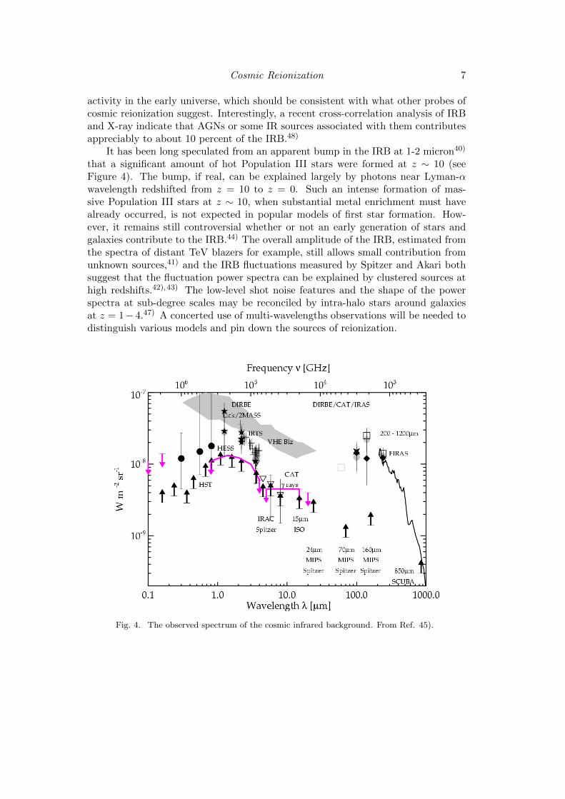
It has been long speculated from an apparent bump in the IRB at 1-2 micron40)

that a significant amount of hot Population III stars were formed at z ∼ 10 (seeFigure 4). The bump, if real, can be explained largely by photons near Lyman-αwavelength redshifted from z = 10 to z = 0. Such an intense formation of mas-sive Population III stars at z ∼ 10, when substantial metal enrichment must havealready occurred, is not expected in popular models of first star formation. How-ever, it remains still controversial whether or not an early generation of stars andgalaxies contribute to the IRB.44) The overall amplitude of the IRB, estimated fromthe spectra of distant TeV blazers for example, still allows small contribution fromunknown sources,41) and the IRB fluctuations measured by Spitzer and Akari bothsuggest that the fluctuation power spectra can be explained by clustered sources athigh redshifts.42), 43) The low-level shot noise features and the shape of the powerspectra at sub-degree scales may be reconciled by intra-halo stars around galaxiesat z = 1− 4.47) A concerted use of multi-wavelengths observations will be needed todistinguish various models and pin down the sources of reionization.

Fig. 4. The observed spectrum of the cosmic infrared background. From Ref. 45).


§6. Probes of reionization

From observations of the spectra of distant quasars, it is known that the Universeis highly ionized today.2), 55), 56), 57) Evidence for reionization at the 5.5σ level wasobtained by the Wilkinson Microwave Anisotropy Probe (WMAP) measurement ofthe CMB EE polarization power spectrum.58)

Reionization began at a redshift z ∼ 20 − 30 when the first stars were formed.Later, Population II stars, star forming galaxies, and active galactic nuclei completedthe process.59), 60), 61), 62), 63), 64) The precise details of the reionization process are notknown, and must be inferred from observations. Let us now discuss two promisingprobes of reionization - the 21 cm spin flip of neutral hydrogen, and the cosmicmicrowave background.

6.1. Probing the dark ages through 21 cm observations

The nature of the earliest stars is a fascinating topic, but one which is very dif-ficult to study due to the lack of observations. Emission and absorption due to the21 cm spin flip transition of neutral hydrogen have emerged as useful techniques toprobe the epoch of primordial star formation.77), 65), 66), 67), 68), 70), 70), 71), 72), 73) Beforethe formation of the first luminous objects, the spin temperature of neutral hydro-gen is typically close to the CMB temperature at a redshift z ∼ 20 because thegas is not dense enough to collisionally couple the spin temperature to its kinetictemperature.65) The formation of the first stars however, results in the productionof Lyman-α photons which can couple the spin and kinetic temperatures of neutralhydrogen through the Wouthuysen-Field mechanism.74), 75) The kinetic temperatureof the gas Tk ∝ (1 + z)2 is typically lower than the CMB temperature Tγ (whichscales as (1+z)) at z ∼ 20.

The Wouthuysen-Field mechanism sets Ts = Tk, so the turn-on of the first starsproduces a significant decrease in the 21 cm brightness temperature (Tb) around theredshift of first star formation, with Tb ∝ (Ts−Tγ)/Ts ∼ −Tγ/Tk . We thus expect asignificant decrement in the 21 cm brightness temperature Tb around the redshift offirst star formation, since Tb ∝ (Ts−Tγ)/Ts. Heating of the gas by ionizing radiationrapidly sets Tk > Tγ , with Tb entering the saturation regime before decreasing tozero as the Universe reionizes. The magnitude of the decrement in Tb as well asthe width provide valuable information on the properties of the first stars and X-raysources. The spectral structure allows us to distinguish the signal from the muchlarger background which is spectrally smooth.

The 21 cm brightness temperature relative to the CMB (also called differentialbrightness temperature) is given by (see, for example69)):

Tb ≈ 27 mK xHI

√1 + z

10

(1− Tγ

Ts

), (6.1)

where xHI is the neutral hydrogen fraction, and Ts is the spin temperature of neutralhydrogen given by:

T−1s ≈T−1γ + (xc + xα)T−1k

1 + xc + xα. (6.2)


Fig. 5. The large-scale 21 cm fluctuations calculated by SIMFAST. Each panel is 300 Mpc × 300

Mpc, and shows the brightness temperature in Kelvin at z = 14, 12, 10, 8 (from top left to

bottom right).

xc is called the collisional coupling coefficient, while xα is the Lyman-α couplingdue to the Wouthuysen-Field mechanism. Collisional coupling is important when thegas is dense or hot, i.e. at high redshifts. Figure 6(a) shows the collisional couplingand Lyman-α coupling (xα) as functions of redshift (for a particular star formationmodel). Once star formation begins at a redshift z . 30, the Lyman-α couplingprovides the dominant contribution. Figure 6(b) shows the gas kinetic temperaturefor a specific star formation model, as well as the CMB temperature. At very highredshifts (z & 300), the gas temperature closely follows the CMB temperature dueto Compton scattering with residual electrons. At lower redshifts, the gas is notsufficiently dense for Compton scattering to be efficient. The kinetic temperaturethen falls off ∝ (1 + z)2 until star formation begins. Three dimensional maps of thebrightness temperature of neutral Hydrogen can be used to infer the reionizationhistory of the Universe. Fig. 5 shows the simulated brightness temperature (for aparticular star formation model) in 300 Mpc × 300 Mpc boxes at redshifts z = 14,12, 10, and 8, obtained using the SIMFAST code.86)

The intensity of radiation in the Lyman-α wavelength at any given redshift


10−4

10−3

10−2

10−1

1

101

102

10 15 20 25 30

z

1

10

100

1000

10 15 20 25 30

Kel

vin

z

-300

-250

-200

-150

-100

-50

0

50

10 15 20

Tb

(mK

)

z

xc

xα

Tk

Tγ

Tk (no heating)

Model #1Model #2Model #3

(a) (b)

(c)

1

Fig. 6. Panel (a) shows the collisional coupling coefficient compared to the Lyman-α coupling

coefficient. At high redshifts, collisional coupling provides the dominant contribution, but after

first star formation, xα xc. (b) shows the gas kinetic temperature (solid, black) and the CMB

temperature (dashed, red). The dotted (blue) line shows the gas temperature in the absence of

heating. (c) shows the 21 cm brightness temperature (relative to the CMB), for three different

models that differ in their star formation rate, and X-ray flux.

z is due to radiation emitted between the Lyman-α wavelength and the Lymanlimit. Thus radiation emitted at wavelengths shorter than Lyman-α, at a redshiftz′ < zmax(n) will redshift until the photons reach the Lyman-α wavelength at aredshift z < z′. Thus photons with wavelengths between Lyman-α and Lyman-β arevisible up to a maximum redshift zmax(2), where 1+zmax(2) = (λα/λβ)(1+z).80) TheLyman-α coupling coefficient xα is proportional to the Lyman-α photon intensity:80)

Jα =(1 + z)2

4π

nmax∑n=2

∫ zmax(n)

z

cdz′

H(z′)ε(ν ′n, z

′), (6.3)

where ε is the number of photons emitted per comoving volume, per unit time, perfrequency, and depends on the nature of the ionizing sources.


Once the Lyman-α coupling xα 1, the spin temperature Ts is set to thekinetic temperature Tk of the gas. The redshift at which xα > 1 is however, sensitiveto the nature of the ionizing sources. The initial mass function (IMF) of Pop.III plays an important role in determining the number of Lyman-α and ionizingphotons. Authors81) find that a 170 M star emits about 34,500 ionizing photonsper baryon over its lifetime, compared to ≈ 6600 per baryon per lifetime for a Pop.II star. Authors82) find that a heavy IMF with M > 300M produces 16 times asmany ionizing photons compared to a Salpeter IMF. Thus, one may hope to placeconstraints on the nature of Pop. III stars by measuring the brightness temperatureof neutral Hydrogen 21 cm radiation, although it will be challenging to break thedegeneracy between the primordial star IMF and the star formation rate86)

Accretion of gas onto black holes produced by the first stars will generate highlyenergetic X-rays which heat the gas to temperatures above the CMB. The temper-ature evolution of the gas in the presence of X-ray heating is given by:

− (1 + z)H(z)dTkdz

= −2T (z)H(z) +2ηheat(z)

3kbξ(z), (6.4)

in the limit of ionized fraction xion 1. ξ(z) is the energy absorbed per atomper unit time at redshift z. ηheat is the fraction of the absorbed energy that goesinto heating. Detailed computations87), 88), 89), 90) show that ηheat is a function ofphoton energy, as well as the ionized fraction. For highly neutral gas xion ≈ 10−4,we have ηheat . 0.2 for photon energies Eγ > 100 eV. For slightly ionized gas withxion ∼ 0.01, ηheat ∼ 0.4 for Eγ > 100 eV, with lower energy photons contributingmore to heating.87)

The ratio of temperatures in the absence of any heating is approximately givenby Tγ/Tk ≈ 7.66 [20/(1 + z)]. From Eq. 6.1, it is easy to see that the minimum

brightness temperature (relative to the CMB) is ≈ −300√

20/(1 + z) mK, whenthe gas is not heated by X-rays, and when the spin and kinetic temperatures arewell coupled by Lyman-α photons. Figure 6(c) shows the brightness temperature ofneutral hydrogen relative to the CMB, obtained using the SIMFAST code,85), 86) forthree different models that differ in their star formation efficiency and X-ray heatingflux. The location of the trough in Tb, as well as its width are determined by thephysics of primordial star formation, i.e. the Lyman-α, and X-ray flux, which inturn may be related to the star formation efficiency, and X-ray heating rate. It isclear that a precise measurement of the 21 cm temperature will provide importantinformation regarding the formation of the first stars.

6.2. Measuring the global 21 cm brightness temperature

Experiments studying the universe through the 21 cm transition include thePrecision Array for Probing the Epoch of Reionization (PAPER),91), 92) the GiantMetrewave Radio Telescope - Epoch of Reionization (GMRT-EoR),93) the Low Fre-quency Array (LOFAR),94) the Murchison Widefield Array (MWA),95) the HydrogenEpoch of Reionization Array (HERA),96) the Square Kilometer Array (SKA),97) theExperiment to Detect the Global EoR Step (EDGES),98) the Large Aperture Experi-ment to detect the Dark Ages (LEDA),99) the Sonda Cosmologica de las Islas para la


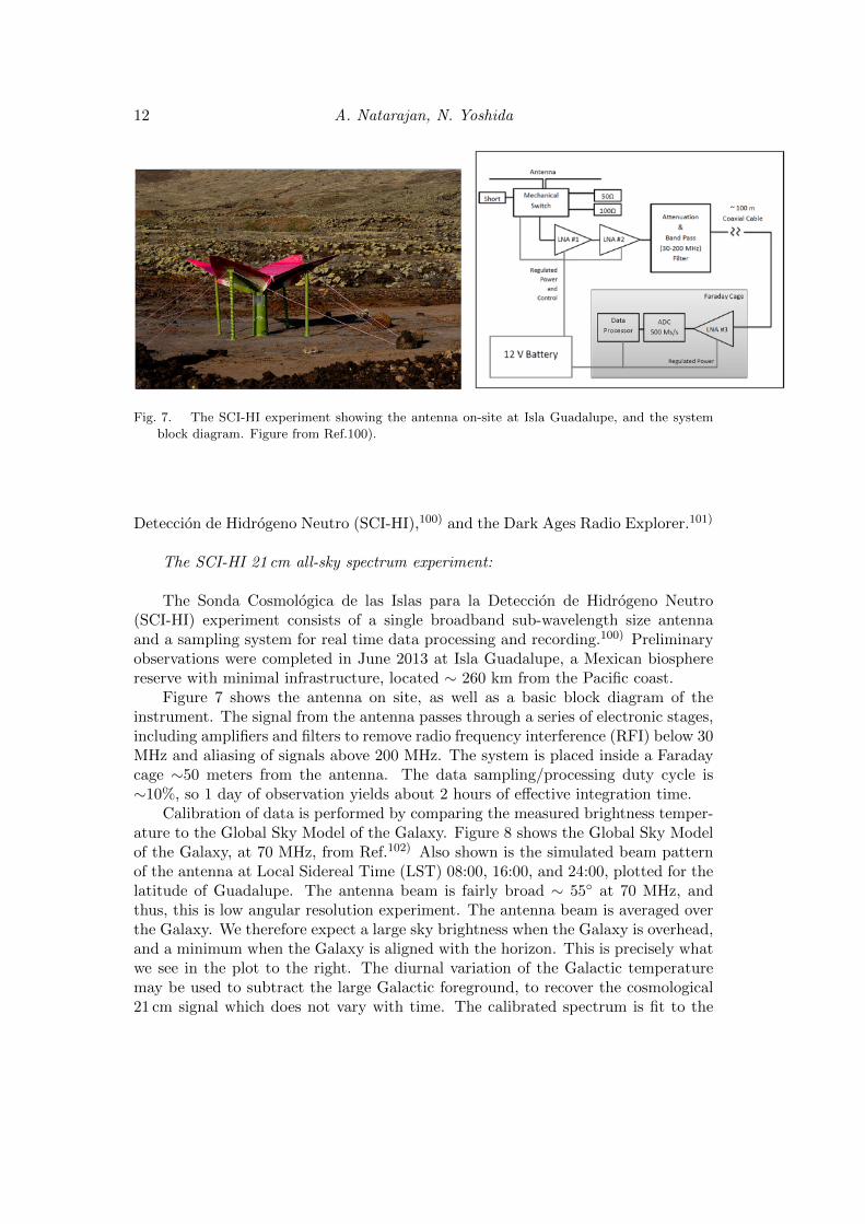
Fig. 7. The SCI-HI experiment showing the antenna on-site at Isla Guadalupe, and the system

block diagram. Figure from Ref.100).

Deteccion de Hidrogeno Neutro (SCI-HI),100) and the Dark Ages Radio Explorer.101)

The SCI-HI 21 cm all-sky spectrum experiment:

The Sonda Cosmologica de las Islas para la Deteccion de Hidrogeno Neutro(SCI-HI) experiment consists of a single broadband sub-wavelength size antennaand a sampling system for real time data processing and recording.100) Preliminaryobservations were completed in June 2013 at Isla Guadalupe, a Mexican biospherereserve with minimal infrastructure, located ∼ 260 km from the Pacific coast.

Figure 7 shows the antenna on site, as well as a basic block diagram of theinstrument. The signal from the antenna passes through a series of electronic stages,including amplifiers and filters to remove radio frequency interference (RFI) below 30MHz and aliasing of signals above 200 MHz. The system is placed inside a Faradaycage ∼50 meters from the antenna. The data sampling/processing duty cycle is∼10%, so 1 day of observation yields about 2 hours of effective integration time.

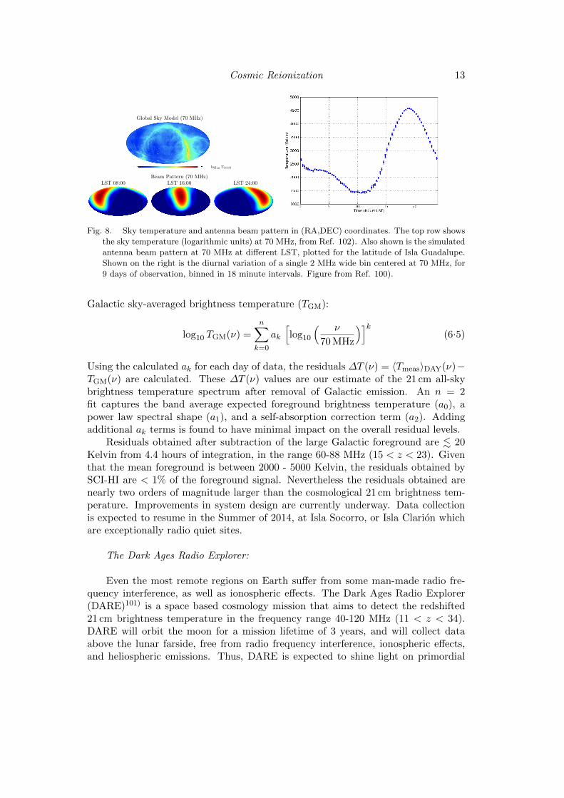
Calibration of data is performed by comparing the measured brightness temper-ature to the Global Sky Model of the Galaxy. Figure 8 shows the Global Sky Modelof the Galaxy, at 70 MHz, from Ref.102) Also shown is the simulated beam patternof the antenna at Local Sidereal Time (LST) 08:00, 16:00, and 24:00, plotted for thelatitude of Guadalupe. The antenna beam is fairly broad ∼ 55 at 70 MHz, andthus, this is low angular resolution experiment. The antenna beam is averaged overthe Galaxy. We therefore expect a large sky brightness when the Galaxy is overhead,and a minimum when the Galaxy is aligned with the horizon. This is precisely whatwe see in the plot to the right. The diurnal variation of the Galactic temperaturemay be used to subtract the large Galactic foreground, to recover the cosmological21 cm signal which does not vary with time. The calibrated spectrum is fit to the


1

Global Sky Model (70 MHz)

log10 TGSM

Beam Pattern (70 MHz)LST 08:00 LST 16:00 LST 24:00

08:00 LST 16:00 LST 24:00 LST

1

2000

3000

4000

5000

10 12 14 16 18 20 22 24

Sky

Tem

per

atu

re[K

elvin

]

Hours LST

60 65 70 75 80 85 90

Frequency (MHz)

Calibrated DataGSM Beam(t)

1

-2

-1.5

-1

-0.5

0

0.5

1

1.5

2

60 65 70 75 80 85 90

22.67 20.85 19.29 17.93 16.75 15.71 14.78

Com

bin

edR

esid

uals

(Kel

vin

)

Frequency (MHz)

Redshift

1

Fig. 8. Sky temperature and antenna beam pattern in (RA,DEC) coordinates. The top row shows

the sky temperature (logarithmic units) at 70 MHz, from Ref. 102). Also shown is the simulated

antenna beam pattern at 70 MHz at different LST, plotted for the latitude of Isla Guadalupe.

Shown on the right is the diurnal variation of a single 2 MHz wide bin centered at 70 MHz, for

9 days of observation, binned in 18 minute intervals. Figure from Ref. 100).

Galactic sky-averaged brightness temperature (TGM):

log10 TGM(ν) =

n∑k=0

ak

[log10

( ν

70 MHz

)]k(6.5)

Using the calculated ak for each day of data, the residuals ∆T (ν) = 〈Tmeas〉DAY(ν)−TGM(ν) are calculated. These ∆T (ν) values are our estimate of the 21 cm all-skybrightness temperature spectrum after removal of Galactic emission. An n = 2fit captures the band average expected foreground brightness temperature (a0), apower law spectral shape (a1), and a self-absorption correction term (a2). Addingadditional ak terms is found to have minimal impact on the overall residual levels.

Residuals obtained after subtraction of the large Galactic foreground are . 20Kelvin from 4.4 hours of integration, in the range 60-88 MHz (15 < z < 23). Giventhat the mean foreground is between 2000 - 5000 Kelvin, the residuals obtained bySCI-HI are < 1% of the foreground signal. Nevertheless the residuals obtained arenearly two orders of magnitude larger than the cosmological 21 cm brightness tem-perature. Improvements in system design are currently underway. Data collectionis expected to resume in the Summer of 2014, at Isla Socorro, or Isla Clarion whichare exceptionally radio quiet sites.

The Dark Ages Radio Explorer:

Even the most remote regions on Earth suffer from some man-made radio fre-quency interference, as well as ionospheric effects. The Dark Ages Radio Explorer(DARE)101) is a space based cosmology mission that aims to detect the redshifted21 cm brightness temperature in the frequency range 40-120 MHz (11 < z < 34).DARE will orbit the moon for a mission lifetime of 3 years, and will collect dataabove the lunar farside, free from radio frequency interference, ionospheric effects,and heliospheric emissions. Thus, DARE is expected to shine light on primordial


star formation: in particular DARE expects to place useful bounds on the epoch offirst star formation, the formation of the first accreting black holes, and the start ofthe reionization epoch.

The DARE radiometer consists of a dual-polarized antenna with a compact,integrated, front-end electronics package, a single-band, dual-channel receiver, anda digital spectrometer. The antenna consists of a pair of bi-conical dipoles, madeunidirectional by a set of deployable radials attached to the spacecraft bus that actas an effective ground plane. The receiver provides amplification of the antennasignal to a level sufficient for further processing by the digital spectrometer, andincorporates a load switching scheme to assist calibration. There are two receivers toaccommodate the antennas, i.e. one receiver per antenna polarization. Noise diodesprovide a reliable additive noise temperature during operation. The noise diodes willbe used to monitor spectral response and linearity of downstream components. Theinstrument design is coupled to a multi-tiered calibration strategy to obtain the RFspectra from which the 21 cm signal can be extracted. The calibration strategy relieson the fact that a high degree of absolute calibration is not required, but focuses onthe relative variations between spectral channels, which are much easier to control.

The antenna power pattern covers approximately 1/8 of the sky depending onfrequency, and the data set will consist of spectra from 8 independent regions onthe sky. DARE uses four free parameters to fit the foreground, i.e. log TFG =log T0 + a1 log ν + a2 (log ν)2 + a3 (log ν)3. The parameter values are fit separately,to each sky region. Thus, there are 32 foreground parameters in total. It is pos-sible to separate the signal from the large foregrounds because the foregrounds arespectrally smooth, while the 21 cm brightness temperature has spectral structure.Also the foregrounds are spatially varying, while the 21 cm temperature is spatiallysmooth. With three years of observation, the DARE mission is expected to obtain3000 hours of integration. The experiment is expected to constrain the epoch of firststar formation to ∼ 9% accuracy, the start of X-ray heating by accreting black holesto ∼ 1.4% accuracy, and the start of reionization to ∼ 0.4% accuracy.

Both SCI-HI and DARE expect to measure the global 21 cm signal. The powerspectrum of 21 cm fluctuations is also a useful tool to study reionization. There existfluctuations in the 21 cm brightness temperature due to fluctuations in the matterdensity, neutral fraction, and temperature. Fluctuations in the 21 cm brightnesstemperature are expected to be large near the edges of HI regions, and thereforemay be more easily separated from the large Galactic foreground compared to theglobal signal, particularly near the end of reionization. The fluctuation in the bright-ness temperature δ21 = δTb/Tb is caused by fluctuations in the density field δ, theneutral fraction δHI, the Lyman-α flux δα, the radial velocity gradient δdrvrand thetemperature δT:105)

δ21 =

[1 +

xcxtot(1 + xtot)

]δ +

xαxtot(1 + xtot)

δα + δHI

− δdrvr + δT

(Tk

Tk − Tγ+

xαxtot(1 + xtot)

d log κ10d log Tk

), (6.6)

where xtot = xc+xα, and κ10(Tk) is the collisional spin de-excitation rate coefficient.


1000

2000

3000

4000

5000

6000

100 200 300 400 500 600 700 800 900 1000

(+

1)C

TT

/2(µ

K2)

= 0.08 = 0.10 = 0.12

1

0

0.02

0.04

0.06

0.08

0.1

0.12

0.14

0.16

0.18

2 4 6 8 10 12 14

(+

1)C

EE

/2(µ

K2)

= 0.08 = 0.10 = 0.12

1

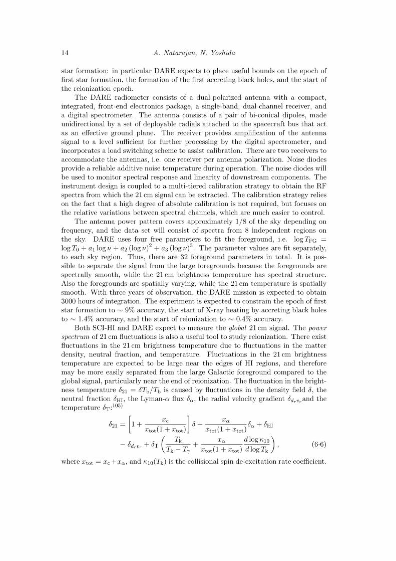
Fig. 9. CMB power spectra - TT and EE for different values of τ . Scattering of CMB photons

with free electrons results in a damping in the TT power spectrum, and a boost in the large

angle EE power spectrum proportional to τ2.

The fluctuations in Fourier space may be expressed in the form:105)

δTb(~k) = µ2δ(~k) + βδ(~k) + δrad(~k), (6.7)

where µ is the cosine of the angle between the wave vector ~k and the line of sight,while β is obtained by collecting together the terms in Eq. 6.6. Early results onreionization have been obtained by the PAPER experiment92) using the power spec-trum of 21 cm observations. The PAPER experiment consists of 32 antennas, andcollects data in South Africa. With an exposure of 55 days, PAPER obtained anupper limit on the 21 cm power spectrum of (52mK)2 for k = 0.11 h/Mpc at z=7.7at the 2σ level.

§7. Probing reionization with the cosmic microwave background

So far, we have discussed how the highly redshifted 21 cm radiation from neutralHydrogen can probe early reionization. The cosmic microwave background is alsoan excellent probe of reionization. This is because free electrons scatter microwavephotons, modifying the spectrum of anisotropies, and generating new, secondaryanisotropies.

Scattering of CMB photons by free electrons leads to a damping in the temper-ature power spectrum by a factor exp [−2τ ]. Unfortunately, this damping is largelydegenerate with the amplitude of the primordial curvature power spectrum (As or∆2

R). This degeneracy is broken by polarization. Thomson scattering polarizes theCMB, and hence leads to a boost in the large angle EE power spectrum. Figure9 shows the TT and EE power spectra for three different values of τ . The Planckexperiment (with WMAP polarization data included) has obtained a value of opticaldepth τ = 0.089+0.012

−0.014. The mean redshift of reionization is then z∗ = 11.1±1.1. Theduration of reionization is however, not well constrained by the polarization powerspectrum.

Secondary scattering of CMB photons introduces additional power on smallscales. High energy photons emitted from luminous sources ionize the region around


0

0.2

0.4

0.6

0.8

1

6 7 8 9 10 11 12 13 14

xe(z

)

z

0.01

0.1

1

2000 3000 4000 5000

l(l+

1)C

EE

l/2

(µK

2)

l

Patchy

Patchy kSZ

(a) (b)

= 0.083, RMS = 0.0027 = 0.086, RMS = 0.0030 = 0.081, RMS = 0.0022

`(`+

1)C

TT

`/2

(µK

2)

0

0.2

0.4

0.6

0.8

1

6 7 8 9 10 11 12 13 14

xe(z

)

z

0.01

0.1

1

2000 3000 4000 5000

l(l+

1)C

EE

l/2

(µK

2)

l

Patchy

Patchy kSZ

(a) (b)

= 0.083, RMS = 0.0027 = 0.086, RMS = 0.0030 = 0.081, RMS = 0.0022

1

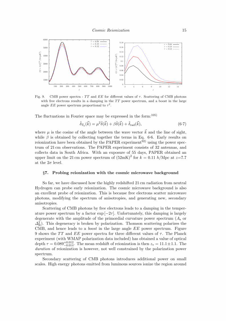
Fig. 10. Shown are three different reionization scenarios that have the same mean redshift of

reionization, but different values of 〈τ〉 and τRMS. The plot on the right shows the corresponding

kSZ power spectra, and patchy τ power spectra. From Ref. 112)

the sources, forming bubbles of hot ionized gas. Reionization is then said to bepatchy, and the optical depth becomes a function of direction, i.e. τ = τ(n), and canbe described to lowest order by 2 quantities: the mean over angles 〈τ〉, and the vari-ance over angles, or equivalently, the root mean square value τRMS. In the presenceof a patchily reionized Universe, one observes a different CMB temperature whenthe line of sight passes through an ionized region, compared to a neutral region. Ananisotropic optical depth therefore introduces “patchy screening” of the CMB, andhence secondary CMB power on small scales.

CMB photons scattering off moving electrons also introduces power on smallscales, the well known Sunyaev-Zeldovich effect.106), 107) When the electron velocityis due to thermal motion of gas atoms, it is known as the thermal Sunyaev-Zeldovich(tSZ) effect. The main contribution to the tSZ power comes from galaxy clusters.Scattering of CMB photons by free electrons with a bulk velocity (i.e. velocityrelative to the Hubble flow) results in the kinetic Sunyaev-Zeldovich (kSZ) power.The fractional temperature change induced by electrons with a bulk motion alongthe line of sight is:108), 109)

∆T

T= −

∫cdt

(n · ~v

c

)neσTe

−τ , (7.1)

where n is a unit vector denoting the line of sight, ~v is the peculiar velocity of theelectrons, ne is the number density of free electrons, σT is the Thomson cross section,and τ is the optical depth. The homogeneous, linear contribution to the kSZ is calledthe Ostriker-Vishniac effect.108), 109) In this approximation, the peculiar velocity ~vmay be simply expressed in terms of the matter overdensity. The Ostriker-Vishniacpower spectrum may then be analytically computed (see for e.g.,110) and111)). Thetotal kSZ is almost always larger than the Ostriker-Vishniac power due to non-linearities, and patchiness in the reionization field. The patchy component of the kSZdue to a patchily reionized Universe is a good probe of the duration of reionization.


Figure 10 (left) shows three different non-instantaneous reionization scenarios,assuming single step reionization (from Ref.112)). These three reionization historieshave the same mean reionization redshift, but different mean values 〈τ〉, as wellas different durations, and hence different values of τRMS. The short reionizationscenario has 〈τ〉 = 0.081, τRMS = 0.0022, the fiducial model has 〈τ〉 = 0.083, τRMS =0.0027, and the extended reionization model has 〈τ〉 = 0.086, τRMS = 0.0030. Thesevalues of τRMS are representative of what is seen in realistic numerical simulations.The plot on the right shows the corresponding values of patchy kSZ as well as excesspower due to patchy τ , for the three reionization models. Using large scale numericalsimulations, authors113), 114) found an approximate scaling relation for the patchy kSZpower:

DkSZ`=3000 ≈ 2.02µK2

[(1 + z

11

)− 0.12

](∆z

1.05

)0.47

, (7.2)

where D` = l(l + 1)Cl/2π, and ∆z = [z(xe = 25%)− z(xe = 75%)].

7.1. Detecting patchy reionization through cross correlation of the CMB

Let us now consider a different technique to probe patchy reionization. Since thedamping term exp [−τ(n)] multiplies the primary CMB temperature T , the effectof patchy reionization is largest when |T | is large, i.e. on degree scales. Patchyreionization therefore transfers CMB power from large scales to small scales. Thisresults in a non-zero correlation between large and small scales. This “patchy τcorrelator” is far more sensitive to patchy reionization than the power spectrum.

To compute the patchy τ correlator, we begin by filtering the CMB into 2 maps:(i) A map with information only on large scales, i.e. multipoles ` < `boundary1, and(ii) A map with information only on small scales, ` > `boundary2. The 2 maps are thensquared: f = T 2(` < `boundary1), g = T 2(` > `boundary2). The patchy τ correlatoris then simply 〈δfδg〉, where δf = f − 〈f〉, and δg = g − 〈g〉 are fluctuations inthe squared CMB temperature obtained from the filtered maps. The angle bracketsdenote an average over the map. Let us first examine a simple model wherein weignore all secondaries besides patchy reionization. Let θobs(n) be the observed CMBtemperature fluctuation, and let θcmb(n) be the primordial CMB fluctuation. θcmb

consists of large scale and small scale modes, i.e. θcmb = θL + θS. The optical depthis τ(n) = 〈τ〉+ δτ(n) .

The observed fluctuation is then given by θobs(n) = θcmb(n) × exp [−δτ(n)] ≈θcmb(n) − δτ(n)θcmb(n), where we have dropped the constant term exp [−〈τ〉] be-cause it is an overall multiplicative constant. The δτ(n) fluctuations are on scalesmuch smaller than the primary CMB fluctuations. When the observed CMB mapis filtered, we obtain a large scale map θL, and a small scale map θS + θLδτ . Thelarge scale and small scale modes of the CMB are independent of each other, andare therefore uncorrelated. The δτ(n) field is also uncorrelated with the CMB fluc-tuations. The patchy τ correlator is therefore simply 〈δfδg〉 = 〈δτ2〉×

(〈θ4L〉 − 〈θ2L〉

).

The patchy τ correlator is thus sensitive to optical depth fluctuations and vanishesin the limit of homogeneous reionization.

Figure 11 (from Ref. 112)) shows the patchy τ correlator in units of µK4, with


7

-500

0

500

1000

1500

+ lensing + kSZ (short)

+ patchy τ

+ lensing + kSZ (fid)

+ patchy τ

+ lensing + kSZ (long)

+ patchy τ

(a)

-500

0

500

1000

1500

+ lensing + kSZ (short) + noise

+ patchy τ

noise RMS = 5 µK, threshold = ± 25 µK

+ lensing + kSZ (fid) + noise

+ patchy τ

+ lensing + kSZ (long) + noise

+ patchy τ

(b)

-500

0

500

1000

1500

+lens.+kSZ(short)+tSZ+CIB+radio

+ patchy τ

148 GHz

+lens.+kSZ(fid)+tSZ+CIB+radio

+ patchy τ

+lens.+kSZ(long)+tSZ+CIB+radio

+ patchy τ

(c)

-500

0

500

1000

1500


+ patchy τ

90 GHz


+ patchy τ


+ patchy τ

(d)

500 1000 1500 2000 500 1000 1500 2000 500 1000 1500 2000

lboundary1

Fig. 5.— The patchy τ correlator as a function of lboundary1. The top row (a) includes only frequency independent components, namelyCMB lensing and kSZ, for the three different reionization histories considered in Figure 3. Patchy τ can be detected at high confidence,and the magnitude of the correlator can be used to constrain extended reionization histories. Row (b) shows the patchy τ correlator withgaussian noise included, to account for residuals after frequency dependent secondaries have been subtracted. Patchy τ may be detected ifthe residuals are smaller than ≈ 5 µK. Rows (c) and (d) include the tSZ, CIB, and radio background at frequencies 148 GHz and 90 GHzrespectively, for the three different reionization histories. A statistically significant detection of patchy τ can only be made if these largesecondaries are minimized by a multi-frequency analysis. Zero correlation is shown for reference (thin broken line).

7

-500

0

500

1000

1500

+ lensing + kSZ (short)

+ patchy τ

+ lensing + kSZ (fid)

+ patchy τ

+ lensing + kSZ (long)

+ patchy τ

(a)

-500

0

500

1000

1500

+ lensing + kSZ (short) + noise

+ patchy τ

noise RMS = 5 µK, threshold = ± 25 µK

+ lensing + kSZ (fid) + noise

+ patchy τ

+ lensing + kSZ (long) + noise

+ patchy τ

(b)

-500

0

500

1000

1500


+ patchy τ

148 GHz


+ patchy τ


+ patchy τ

(c)

-500

0

500

1000

1500


+ patchy τ

90 GHz


+ patchy τ


+ patchy τ

(d)

500 1000 1500 2000 500 1000 1500 2000 500 1000 1500 2000

lboundary1

Fig. 5.— The patchy τ correlator as a function of lboundary1. The top row (a) includes only frequency independent components, namelyCMB lensing and kSZ, for the three different reionization histories considered in Figure 3. Patchy τ can be detected at high confidence,and the magnitude of the correlator can be used to constrain extended reionization histories. Row (b) shows the patchy τ correlator withgaussian noise included, to account for residuals after frequency dependent secondaries have been subtracted. Patchy τ may be detected ifthe residuals are smaller than ≈ 5 µK. Rows (c) and (d) include the tSZ, CIB, and radio background at frequencies 148 GHz and 90 GHzrespectively, for the three different reionization histories. A statistically significant detection of patchy τ can only be made if these largesecondaries are minimized by a multi-frequency analysis. Zero correlation is shown for reference (thin broken line).

24N

.Yosh

ida,A

.N

ata

raja

n

7

-5000

500

1000

1500

+le

nsi

ng

+kSZ

(short

)

+patc

hy

+le

nsi

ng

+kSZ

(fid)

+patc

hy

+le

nsi

ng

+kSZ

(long)

+patc

hy

(a) -5

000

500

1000

1500

+le

nsi

ng

+kSZ

(short

)+

nois

e

+patc

hy

nois

eR

MS

=5

µK

,th

resh

old

=±

25

µK

+le

nsi

ng

+kSZ

(fid)

+nois

e

+patc

hy

+le

nsi

ng

+kSZ

(long)

+nois

e

+patc

hy

(b)

-5000

500

1000

1500

+le

ns.

+kSZ(s

hort

)+tS

Z+

CIB

+ra

dio

+patc

hy

148

GH

z

+le

ns.

+kSZ(fi

d)+

tSZ+

CIB

+ra

dio

+patc

hy

+le

ns.

+kSZ(long)+

tSZ+

CIB

+ra

dio

+patc

hy

(c) -5

000

500

1000

1500

+le

ns.

+kSZ(s

hort

)+tS

Z+

CIB

+ra

dio

+patc

hy

90

GH

z

+le

ns.

+kSZ(fi

d)+

tSZ+

CIB

+ra

dio

+patc

hy

+le

ns.

+kSZ(long)+

tSZ+

CIB

+ra

dio

+patc

hy

(d)

500

1000

1500

2000

500

1000

1500

2000

500

1000

1500

2000

l boundary

1

Fig

.5.—

The

patc

hy

corr

elato

ras

afu

nct

ion

ofl b

oundary

1.

The

top

row

(a)

incl

udes

only

freq

uen

cyin

dep

enden

tco

mponen

ts,nam

ely

CM

Ble

nsi

ng

and

kSZ,fo

rth

eth

ree

di

eren

tre

ioniz

ation

his

tori

esco

nsi

der

edin

Fig

ure

3.

Patc

hy

can

be

det

ecte

dat

hig

hco

nfiden

ce,

and

the

magnitude

ofth

eco

rrel

ato

rca

nbe

use

dto

const

rain

exte

nded

reio

niz

ation

his

tori

es.

Row

(b)

show

sth

epatc

hy

corr

elato

rw

ith

gauss

ian

nois

ein

cluded

,to

acc

ount

for

resi

duals

aft

erfr

equen

cydep

enden

tse

condari

eshav

ebee

nsu

btr

act

ed.

Patc

hy

may

be

det

ecte

dif

the

resi

duals

are

smaller

than

5µK

.R

ows

(c)

and

(d)

incl

ude

the

tSZ,C

IB,and

radio

back

gro

und

at

freq

uen

cies

148

GH

zand

90

GH

zre

spec

tivel

y,fo

rth

eth

ree

di

eren

tre

ioniz

ation

his

tori

es.

Ast

atist

ically

signifi

cant

det

ection

of

patc

hy

can

only

be

made

ifth

ese

larg

ese

condari

esare

min

imiz

edby

am

ulti-fr

equen

cyanaly

sis.

Zer

oco

rrel

ation

issh

own

for

refe

rence

(thin

bro

ken

line)

.

7

-5000

500

1000

1500

+le

nsi

ng

+kSZ

(short

)

+patc

hy

+le

nsi

ng

+kSZ

(fid)

+patc

hy

+le

nsi

ng

+kSZ

(long)

+patc

hy

(a) -5

000

500

1000

1500

+le

nsi

ng

+kSZ

(short

)+

nois

e

+patc

hy

nois

eR

MS

=5

µK

,th

resh

old

=±

25

µK

+le

nsi

ng

+kSZ

(fid)

+nois

e

+patc

hy

+le

nsi

ng

+kSZ

(long)

+nois

e

+patc

hy

(b)

-5000

500

1000

1500

+le

ns.

+kSZ(s

hort

)+tS

Z+

CIB

+ra

dio

+patc

hy

148

GH

z

+le

ns.

+kSZ(fi

d)+

tSZ+

CIB

+ra

dio

+patc

hy

+le

ns.

+kSZ(long)+

tSZ+

CIB

+ra

dio

+patc

hy

(c) -5

000

500

1000

1500

+le

ns.

+kSZ(s

hort

)+tS

Z+

CIB

+ra

dio

+patc

hy

90

GH

z

+le

ns.

+kSZ(fi

d)+

tSZ+

CIB

+ra

dio

+patc

hy

+le

ns.

+kSZ(long)+

tSZ+

CIB

+ra

dio

+patc

hy

(d)

500

1000

1500

2000

500

1000

1500

2000

500

1000

1500

2000

l boundary

1

Fig

.5.—

The

patc

hy

corr

elato

ras

afu

nct

ion

ofl b

oundary

1.

The

top

row

(a)

incl

udes

only

freq

uen

cyin

dep

enden

tco

mponen

ts,nam

ely

CM

Ble

nsi

ng

and

kSZ,fo

rth

eth

ree

di

eren

tre

ioniz

ation

his

tori

esco

nsi

der

edin

Fig

ure

3.

Patc

hy

can

be

det

ecte

dat

hig

hco

nfiden

ce,

and

the

magnitude

ofth

eco

rrel

ato

rca

nbe

use

dto

const

rain

exte

nded

reio

niz

ation

his

tori

es.

Row

(b)

show

sth

epatc

hy

corr

elato

rw

ith

gauss

ian

nois

ein

cluded

,to

acc

ount

for

resi

duals

aft

erfr

equen

cydep

enden

tse

condari

eshav

ebee

nsu

btr

act

ed.

Patc

hy

may

be

det

ecte

dif

the

resi

duals

are

smaller

than

5µK

.R

ows

(c)

and

(d)

incl

ude

the

tSZ,C

IB,and

radio

back

gro

und

at

freq

uen

cies

148

GH

zand

90

GH

zre

spec

tivel

y,fo

rth

eth

ree

di

eren

tre

ioniz

ation

his

tori

es.

Ast

atist

ically

signifi

cant

det

ection

of

patc

hy

can

only

be

made

ifth

ese

larg

ese

condari

esare

min

imiz

edby

am

ulti-fr

equen

cyanaly

sis.

Zer

oco

rrel

ation

issh

own

for

refe

rence

(thin

bro

ken

line)

.

Fig

.7.

Fig

.7

show

sth

epat

chy

corr

elato

rin

unit

sof

µK

4,w

ith

and

wit

hout

pat

chy

reio

niz

ati

on.

The

CM

Bm

apsw

ere

sim

ula

ted

usi

ng

the

HE

ALP

IXso

ftw

are.

The

patc

hy

reio

niz

ati

on

map

was

obta

ined

usi

ng

num

eric

alsi

mula

tions.

The

boundar

yfo

rth

ela

rge

scal

em

apl b

oundary

1is

vari

edfr

om50

0-

2000

.T

he

smal

lsc

ale

map

incl

udes

mult

ipole

sfr

om300

0-50

00.

The

map

ssh

own

inFig

.7

incl

ude

kSZ

and

lensi

ng,

but

do

not

incl

ude

tSZ,C

IB,or

radio

contr

ibuti

ons.

The

thre

epan

els

are

plo

tted

for

the

3re

ioniz

atio

nsc

enar

ios

show

nin

Fig

.6.

The

short

reio

niz

atio

nsc

enar

iohashi=

0.081,

RM

S=

0.00

22,th

efiduci

alm

odel

hashi=

0.0

83, R

MS

=0.

0027,

and

the

exte

nded

reio

niz

atio

nm

odel

has

hi=

0.0

86,

RM

S=

0.0

030.

Sin

cedi↵

eren

tm

ult

ipol

esof

the

pri

mary

CM

Bpro

vid

ein

dep

enden

tin

form

atio

n,

the

corr

elat

ion

bet

wee

nla

rge

and

small

scal

em

aps

isze

rofo

rth

epri

mary

CM

B.

Incl

udin

gth

ee↵

ect

ofC

MB

lensi

ng

how

ever

resu

lts

ina

non-z

ero

cros

sco

rrel

atio

n,

bec

ause

lensi

ng

ofth

eC

MB

resu

lts

ina

redis

trib

uti

onof

pow

er,tr

ansf

erri

ng

CM

Bpow

erfr

omla

rge

scal

esto

smal

lsc

ale

s.T

he

cros

sco

rrel

atio

ndue

tole

nsi

ng

isneg

ati

vefo

rsm

alll b

oundary

1,and

incr

ease

s,pass

ing

thro

ugh

zero

atl b

oundary

1

1200.

The

pat

chy

te

rmis

sim

ilar

lyco

rrel

ated

.T

he

cross

corr

elati

ondue

topat

chy

is

alw

ays

pos

itiv

eand

incr

ease

sw

ith

l boundary

1.

Mor

eover

the

patc

hy

term

sco

ntr

ibute

ssi

gnifi

cantl

ym

ore

toth

ecr

oss

corr

elat

ion

than

the

lensi

ng

term

.T

hus,

wit

hon

lyth

ele

nsi

ng

and

kSZ

contr

ibuti

ons,

one

can

det

ect

pat

chy

reio

niz

atio

nat

hig

hsi

gnifi

cance

by

com

puti

ng

the

cross

corr

elati

on

bet

wee

nth

esq

uar

edm

aps.

Ack

now

ledgem

ents

The

pre

sent

work

issu

ppor

ted

inpar

tby

the

Gra

nts

-in-A

idby

the

Min

istr

yof

Educa

tion

,Sci

ence

and

Cult

ure

of

Jap

an(2

16840

7,21

24402

1:K

O,

2067

4003:

NY

).T

Hack

now

ledge

ssu

ppor

tby

Fel

low

ship

ofth

eJap

anSoci

ety

for

the

Pro

moti

on

ofSci

ence

for

Res

earc

hA

bro

ad.

A.N

.w

asfu

nded

by

NA

SA

grant

..

..A

.N.ac

know

l-ed

ges

part

ial

finan

cial

suppor

tfr

om

the

Pit

tsburg

hPar

ticl

ephysi

cs,

Ast

rophysi

cs,

and

Cosm

olog

yC

ente

r,an

dth

eD

epar

tmen

tofP

hysi

csand

Ast

ronom

yat

the

Uni-

Fig. 11. The patchy τ correlator for different reionization scenarios. The CMB maps were obtained

using HEALPIX,118) and the patchy τ maps were obtained from numerical simulations.113) Only

kSZ and lensing have been included. It is easy to distinguish even small values of patchy τ when

the larger secondary components have been removed through a multi-frequency analysis. From

Ref. 112).

and without patchy reionization. The CMB maps were simulated using the HEALPix

software.118) The patchy reionization map was obtained using numerical simulations.The boundary for the large scale map lboundary1 is varied from 500 - 2000. Thesmall scale map includes multipoles from 3000-5000. The maps shown in Figure11 include kSZ and lensing, but do not include tSZ, CIB, or radio contributions.Thus, we assume that the large frequency dependent contaminations may be removedthrough a multi-frequency analysis of the data. The three panels are plotted for the3 reionization scenarios shown in Figure 10.

Since different multipoles of the primary CMB provide independent information,the correlation between large and small scale maps is zero for the primary CMB. In-cluding the effect of CMB lensing however results in a non-zero cross correlation,because lensing of the CMB results in a redistribution of power, transferring CMBpower from large scales to small scales. The cross correlation due to lensing is neg-ative for small lboundary1, and increases, passing through zero at lboundary1 ∼ 1200.The patchy τ term is similarly correlated. The cross correlation due to patchy τis always positive and increases with lboundary1. Moreover the patchy τ terms con-tributes significantly more to the cross correlation than the lensing term. Thus, onecan detect patchy reionization at high significance by computing the cross correla-tion between the squared maps. It is however, much harder to measure the patchyτ correlator when other secondaries such as tSZ, CIB, and radio contributions arepresent.112)

§8. Future prospects

A number of observational programs are aimed at detecting the signatures ofreionization in the CMB. Data from the Planck mission will deliver accurate mea-surement of the CMB polarization and the total Thomson optical depth, from which


details of reionization can be derived.53), 54) Ongoing experiments such as ACTPol116)

and SPTPol117) will be able to measure the kinematic Sunyaev-Zeldovich effect tohigher accuracy. The Cosmology Large Angular Scale Surveyor (CLASS)123) andthe Primordial Inflation Polarization Explorer (PIPER)124) are designed to measurethe primordial B mode polarization of the CMB, but they will also have the sensi-tivity to measure the E mode to very high accuracy. The CLASS instrument hasa field of view of 19 × 14 with a resolution of 1.5 FWHM, and will measure thepolarization of the CMB at 40, 90, and 150 GHz from Cerro Toco in the Atacamadesert of northern Chile. PIPER is a balloon based experiment, and will fly in boththe northern and southern hemispheres, achieving a sky coverage of 85%. With 5120detectors, PIPER is expected to obtain noise residuals less than 2.7 nK with 100hours of observation. These experiments will significantly improve our understand-ing of the reionization history of the Universe through precise measurements of thelarge angle polarization of the CMB.

Future observations of the CMB spectral distortion will open a new windowto probe the characteristic spectral energy distribution of the dominant sources ofreionization, e.g. by the Primordial Inflation Explorer (PIXIE),125) and the PolarizedRadiation Imaging and Spectroscopy Mission (PRISM).119) Heating of gas by earlystars results in a Compton-y distortion proportional to the temperature of the gasand the reionization optical depth. PIXIE is expected to measure the Comptondistortion to an accuracy y < 2×10−9. In combination with PIXIE’s measurement ofthe optical depth, PIXIE can determine the temperature of the intergalactic mediumto 5% precision at z=11.125) In fact any form of energy injection to the CMB can bestudied to unprecedented accuracy, and hence decay or annihilation of dark matterparticles, for example, can be inferred from the exact shape of the distortion thatencodes the time when dark matter decay/annihilation occurred.122)

The abundances of light element atoms and ions such as OI, NII, CII can bemeasured, in principle, by utilizing the characteristic CMB spectral (frequency-dependent) signatures and angular fluctuations generated by the resonant scatteringand fine structure line emission.120), 121) Assuming that the first sources of light arealso the first sources of the metals, one can trace the early star-formation historyfrom CMB observations.

Altogether, we have very good prospects that there will be significant progressin the study of the Dark Ages in the next two decades, when next-generation radiotelescope arrays and space-borne CMB experiments probe the distribution of theintergalactic gas in the early universe.

Acknowledgements

The present work is supported in part by the Grants-in-Aid by the Ministryof Education, Science and Culture of Japan (25287050: NY). A.N. was funded byNASA grant NNX14AB57G. A.N. acknowledges partial financial support from thePittsburgh Particle physics, Astrophysics, and Cosmology Center, and the Depart-ment of Physics and Astronomy at the University of Pittsburgh. Portions of thisresearch were conducted at the Jet Propulsion Laboratory, California Institute of


Technology, which is supported by the National Aeronautics and Space Administra-tion (NASA).

References

1) J. E. Gunn, B. A. Peterson, ApJ 142, 1633 (1965)2) X. Fan et al. Astron. J., 122, 2833 (2001)3) G. Hinshaw et al., ApJS 208, 19 (2013)4) X. Fan, Research in Astronomy and Astrophysics 12 865 (2012).5) M. F. Morales, J. S. B. Wiythe, ARAA 48 127 (2010).6) D. H. D. Lyth & A. A. Riotto, Physics Reports 314, 1 (1999).7) N. Yoshida, T. Hosokawa, K. Omukai, PTEP, 2012a 305 (2012)8) J. Miralda-Escude, Science 300, 1904 (2003).9) L. Gao, N. Yoshida, T. Abel, C. S. Frenk, A. Jenkins, & V. Springel, M.N.R.A.S. 378,

449 (2007)10) S. Hirano et al. Astrophys. J., 395, 777 (2014)11) M. Tokutani, N. Yoshida, S.-P. Oh, N. Sugiyama, Astrophys. J., 395, 777 (2009)12) H. Park et al. ApJ, 769, 93 (2013)13) S. Zaroubi et al. MNRAS, 425, 2964 (2012)14) T. Greif et al. MNRAS, 399, 639 (2009)15) M. Ricotti, J. P. Ostriker, MNRAS, 352, 547 (2004)16) M. Kuhlen, P. Madau, R. Montgomery, ApJ, 637, 1 (2006)17) J. Miralda-Escude, M. Haehnelt, M. J. Rees, ApJ, 530, 1 (2000)18) M. Valdes, C. Evoli, A. Messinger, A. Ferrara, N. Yoshida, MNRAS, 429, 1705 (2012)19) D. Finkbeiner, S. Galli, T. Lin, T. R. Slatyer, PRD, 85, 3522 (2012)20) C. Shultz, J. Onorbe, K. N. Abazajian, J. S. Bullock, arXiv:1401.376921) N. Yoshida, A. Sokasian, L. Hernquist, and V. Springel, Astrophys. J. 591, L1 (2003)22) V. Bromm, N. Yoshida, ARAA 49, 373 (2011).23) N. Yoshida, T. Abel, L. Hernquist, and N. Sugiyama, Astrophys. J. 592, 645 (2003)24) P. R. Shapiro, K. Ahn, M. A. Alvarez, I. T. Iliev, H. Martel, & D. Ryu, Astrophys. J. 646,

681 (2006)25) R. J. Bouwens et al. Astrophys. J. 765, 16 (2013)26) R. S. Ellis et al. Astrophys. J. 763, 7 (2013)27) B. E. Robertson, R. S. Ellis, J. S. Dunlop, R. J. McLure, D. P. Stark, Nature 468 (2010)

4928) S. Finkelstein et al. Astrophys. J. 758, 93 (2012)29) S.-P. Oh, Astrophys. J. 569, 558 (2001)30) A. Natarajan, D.J. Schwarz, Phys. Rev. D 78, 103524 (2008)31) A. Natarajan, D.J. Schwarz, Phys. Rev. D 80, 043529 (2009)32) A. Natarajan, D.J. Schwarz, Phys. Rev. D 81, 123510 (2010)33) D. Spolyar, K. Freese, P. Gondolo, Phys. Rev. Lett. 100, 051101 (2008)34) F. Iocco, Astrophys. J. 677, L1 (2008)35) A. Natarajan, J.C. Tan, B.W. O’Shea, Brian W., Astrophys. J. 692, 574 (2009)36) S. Hirano, H. Umeda, N. Yoshida, Astrophys. J. 736, 10 (2011)37) S. Galli, F. Iocco, G. Bertone, A. Melchiorri, Phys. Rev. D 80, 023505 (2009)38) A. Natarajan, Phys. Rev. D, 85, 083517 (2012)39) K. Ahn, M.N.R.A.S. 375, 881 (2007)40) T. Matsumoto et al. Astrophys. J. 626 31 (2005)41) F. Aharonian et al. Nature 440 1018 (2006)42) A. Kashlinsky et al. Astrophys. J. 753 63 (2012)43) T. Matsumoto et al. Astrophys. J. 742 124 (2011)44) E. R. Fernandez et al. Astrophys. J. 750 20 (2012)45) H. Dole et al. Astron. Astrophys. 451 417 (2006)46) E. R. Fernandez, S. Zaroubi MNRAS 433 2047 (2013)47) A. Cooray et al. Nature 490 514 (2012)48) N. Cappelluti et al. ApJ 769 68 (2013)49) T. Kitayama, N. Yoshida, H. Susa, and M. Umemura, Astrophys. J. 613, 631 (2004)50) D. Whalen, T. Abel, and M. L. Norman, Astrophys. J. 610, 14 (2004)

http://arxiv.org/abs/1401.3769


51) E. Komatsu et al., Astrophys. J. 192 (2011) 1852) L. Hui & Z. Haiman, Astrophys. J. 596, 9 (2003)53) G. P. Holder et al. Astrophys. J. 595, 13 (2003)54) P. Mukherjee, A. R. Liddle, MNRAS 389, 231 (2008)55) X. Fan et al. Astron. J., 123, 1247 (2002)56) R. H. Becker et al. Astron. J., 122, 2850 (2001)57) L. Pentericci et al. Astron. J., 123, 2151 (2002)58) D. Larson et al. Astrophys. J.S., 192, 16 (2011)59) J. Tumlinson, J. M. Shull, Astrophys. J. 528, L65 (2000)60) A. Loeb, R. Barkana, Ann. Rev. Astron. Astrophys., 39, 19 (2001)61) R. Barkana, A. Loeb, Phys. Rep., 349, 125 (2001)62) J. S. B. Wyithe, A. Loeb, Astrophys. J., 588, L69 (2003)63) Ciardi, B., Ferrara, A., S. D. M. White, M.N.R.A.S., 344, L7 (2003)64) A. Sokasian, N. Yoshida, T. Abel, L. Hernquist, V. Springel, M.N.R.A.S., 350, 47 (2004)65) A. Loeb,, M. Zardarriaga, Phys. Rev. Lett., 92, 211301 (2004)66) A. Cooray, Phys. Rev. D, 70, 063509 (2004)67) S. Bharadwaj, S. S. Ali, M.N.R.A.S., 352, 142 (2004)68) C. L. Carilli, S. R. Furlanetto, F. Briggs, M. Jarvis, S. Rawlings, H. Falcke, New Astron.

Rev. 48, 1029 (2004)69) S. R. Furlanetto, S.-P. Oh, F. Briggs Physics Reports 433 (2006) 18170) S. R. Furlanetto, F. H. Briggs, New Astron. Rev. 48, 1039 (2004)71) J. R. Pritchard, A. Loeb, Phys. Rev. D, 82, 023006 (2010)72) J. R. Pritchard, A. Loeb, Reports on Progress in Physics, 75, 086901 (2012)73) A. Liu, J. R. Pritchard, M. Tegmark, A. Loeb, Phys. Rev. D 87, 043002 (2013)74) S. A. Wouthuysen Astronomical Journal, 57, 31 (1952)75) G. B. Field Proceedings of the IRE, 46, 240 (1958)76) P. A. Shaver, R. A. Windhorst, P. Madau, A.G. de Bruyn, Astron. Astrophys. 345, 380

(1999)77) P. Madau, A. Meiksin, M.J. Rees, Astrophys. J. 475, 429 (1997)78) P. Tozzi, P. Madau, A. Meiksin, M. J. Rees Astrophys. J., 528, 597 (2000)79) A. Liu, J. R. Pritchard, M. Tegmark, A. Loeb, Phys. Rev. D. 87, 043002 (2013)80) R. Barkana, A. Loeb,, Astrophys. J.626, 1 (2005)81) A. L. Muratov, O. Y. Gnedin, N. Y. Gnedin, M. Zemp, Astrophys. J., 773, 19 (2013)82) V. Bromm, R. P. Kudritzki, A. Loeb, Astrophys. J., 552, 464 (2001)83) S. R. Furlanetto, S.-P. Oh, F. H. Briggs, Phys. Rep. 433, 181 (2006)84) A. Mesinger, S. R. Furlanetto, R. Cen, M.N.R.A.S., 411, 955 (2011)85) M. G. Santos, A. Amblard, J. Pritchard, H. Trac, R. Cen, A. Cooray, Astrophys. J., 689,

1 (2008)86) M.G. Santos, L. Ferramacho, M.B. Silva, A. Amblard, A. Cooray, M.N.R.A.S., 406, 2421

(2010)87) S. Furlanetto,R., Stoever, S.J. Mon. Not. R. Astron. Soc. 404, 1869 (2010)88) J.M. Shull, M.E. Van Steenberg Astrophys. J. 298, 268 (1985)89) T. Kanzaki, M. Kawasaki Phys. Rev. D 78, 103004 (2008)90) M. Valdes, C. Evoli, A. Ferrara Mon. Not. R. Astron. Soc. 404, 1569 (2010)91) J.C. Pober, et al., Aastrophys. J., 768, L36 (2013)92) A. R. Parsons, et al. arXiv:1304.4991 (2013)93) G. Paciga et al., M.N.R.A.S., 413, 1174 (2011)94) M. P. van Haarlem et al., Astron. Astrophys., 556, A2 (2013)95) G. Bernardi, et al., ApJ, 771, 105 (2013)96) Hydrogen Epoch of Reionization Array (HERA), http://reionization.org/RFI2 HERA.pdf97) Square Kilometer Array (SKA) http://www.skatelescope.org/98) J. D. Bowman, A. E. E. Rogers, J. N. Hewitt, Astrophys, J., 676, 1 (2008)99) Large Aperture Experiment to detect the Dark Ages (LEDA) http://www.cfa.harvard.edu/LEDA/science.html100) T.C. Voytek, A. Natarajan, J.M.J. Garcıa, J.B. Peterson O. Lopez-Cruz Astrophys. J.

Lett., 782, L9 (2014)101) J.O. Burns, J. Lazio, S. Bale, J. Bowman, R. Bradley, C. Carilli, S. Furlanetto, G. Harker,

A. Loeb, J. Pritchard Advances in Space Research, 49, 433 (2012)102) A. de Oliveira-Costa, M. Tegmark, B.M. Gaensler, J. Jonas Landecker, T. L., Reich, P.


http://reionization.org/RFI2

http://www.skatelescope.org/

http://www.cfa.harvard.edu/LEDA/science.html


M.N.R.A.S. 388, 247 (2008)103) L.J. Greenhill, G. Bernardi, arXiv:1201.1700 (2012)104) M.A. Clark, P.C. La Plante, L.J. Greenhill, arXiv:1107.4264 (2011)105) R. Barkana, A. Loeb,, Astrophys. J. 624, L65 (2005)106) R.A. Sunyaev, Y.B. Zeldovich, Mon. Not. R. Astron. Soc., 190, 413 (1980)107) Y.B. Zeldovich, R.A. Sunyaev, Astrophysics and Space Science, 4, 301 (1969)108) J.P. Ostriker, E.T. Vishniac, Astrophys. J., 306, L51 (1986)109) E.T. Vishniac, Astrophys. J., 322, 597 (1987)110) A.H. Jaffe, M. Kamionkowski, Phys. Rev. D, 58, 043001 (1998)111) K.G. Lee, arXiv:0902.1530 (2009)112) A. Natarajan, N. Battaglia, H. Trac, U.-L. Pen, A. Loeb, Astrophys. J. 776, 82 (2013)113) N. Battaglia, H. Trac, R. Cen, A. Loeb, Astrophys. J., 776, 81 (2013)114) N. Battaglia, A. Natarajan, H. Trac, R. Cen, A. Loeb, Astrophys. J, 776, 83 (2013)115) O. Zahn, et al. Astrophys. J., 756, 65 (2012)116) M.D. Niemack, et al. Society of Photo-Optical Instrumentation Engineers (SPIE) Con-

ference Series, 7741 (2010)117) J.E. Austermann, et al. Society of Photo-Optical Instrumentation Engineers (SPIE) Con-

ference Series, 8452 (2012)118) K.M. Gorski, E. Hivon, A. J. Banday, B.D. Wandelt, F.K. Hansen, M. Reinecke, M.

Bartelmann, Astrophys. J. 622, 759 (2005)119) P. Andre et al. JCAP 02, 006 (2014).120) K. Basu, C. Hernandez-Monteagudo, R. A. Sunyaev, Astron. Astrophys. 416, 447 (2004).121) C. Hernandez-Monteagudo, R. A. Sunyaev, MNRAS 359 597 (2005)122) R. Khatri, R. A. Sunyaev, JCAP 09, 016 (2012)123) J.R.Eimer, C.L. Bennett, D.T. Chuss, T. Marriage, E.J. Wollack, L. Zeng, Society of

Photo-Optical Instrumentation Engineers (SPIE) Conference Series, 8452 (2012)124) A. Kogut, et al., Society of Photo-Optical Instrumentation Engineers (SPIE) Conference

Series, 8452 (2012)125) A. Kogut, D.J. Fixsen, D.T. Chuss, J. Dotson, E. Dwek, M. Halpern, G.F. Hinshaw, S.M.

Meyer, S.H. Moseley, M.D. Seiffert, D.N. Spergel, E.J. Wollack, JCAP 025 (2011)




department of physics, university of tokyo, bunkyo, … · the dark ages of the universe and...

Documents