Holographic Butterfly Effect at Quantum Critical Points

Yi Ling 1,3,4,∗ Peng Liu 1,† and Jian-Pin Wu 2,3‡

1 Institute of High Energy Physics,

Chinese Academy of Sciences, Beijing 100049, China

2 Institute of Gravitation and Cosmology,

Department of Physics, School of Mathematics and Physics,

Bohai University, Jinzhou 121013, China

3 Shanghai Key Laboratory of High Temperature Superconductors, Shanghai, 200444, China

4 School of Physics, University of Chinese Academy of Sciences, Beijing 100049, China

Abstract

When the Lyapunov exponent λL in a quantum chaotic system saturates the bound λL 6 2πkBT ,

it is proposed that this system has a holographic dual described by a gravity theory. In particular,

the butterfly effect as a prominent phenomenon of chaos can ubiquitously exist in a black hole

system characterized by a shockwave solution near the horizon. In this paper we propose that

the butterfly velocity can be used to diagnose quantum phase transition (QPT) in holographic

theories. We provide evidences for this proposal with an anisotropic holographic model exhibiting

metal-insulator transitions (MIT), in which the derivatives of the butterfly velocity with respect

to system parameters characterizes quantum critical points (QCP) with local extremes in zero

temperature limit. We also point out that this proposal can be tested by experiments in the light

of recent progress on the measurement of out-of-time-order correlation function (OTOC).

∗Electronic address: lingy@ihep.ac.cn†Electronic address: liup51@ihep.ac.cn‡Electronic address: jianpinwu@mail.bnu.edu.cn

1

arX

iv:1

610.

0266

9v3

[he

p-th

] 2

3 O

ct 2

017

I. INTRODUCTION

Quantum phase transition (QPT) is one of the essential and difficult topic in condensed

matter theory (CMT). It usually involves strong correlation physics where traditional treat-

ments are inadequate. Holographic duality has been proved a powerful tool to study strongly

correlated system, and has provided many novel insights into strongly correlated problems.

On the other hand, quantum chaos, also as known as butterfly effect, has been attracting

unprecedented attention recently, which set up a bridge among quantum theory, CMT and

holographic gravity. We shall address the connection between QPT and quantum chaos in

holographic framework in this paper.

The butterfly effect states that an initially small perturbation becomes non-negligible

at later time. The out-of-time-order correlation function (OTOC) in quantum systems can

diagnose the butterfly effect by a sudden decay after the scrambling time t∗, which generically

takes the following form,

F (t, ~x) =〈W †(t, ~x)V †(0, 0)W (t, ~x)V (0, 0)〉β〈W (t, ~x)W (t, ~x)〉β〈V (0, 0)V (0, 0)〉β

= 1− αeλL(t−t∗− |~x|vB

)+ · · · , (1)

where W (t, ~x) ≡ eiHtW (0, ~x)e−iHt, and 〈· · · 〉β represents the ensemble average at temper-

ature T = 1/(kBβ). vB is the butterfly velocity, λL is the Lyapunov exponent and the

scrambling time t∗ is the timescale when the commutator [W (t, ~x), V (0, 0)] grows to O(1).

Physically, F (t) describes the spread, or the scrambling of quantum information over the

degrees of freedom across the system. Very importantly, as a characteristic velocity of a

chaotic quantum system, vB sets a bound on the speed of the information propagation [1].

In holographic theories, the butterfly effect has extensively been studied in context [5–

17]. In the study of high energy scattering near horizon and information scrambling of black

holes it is found that the butterfly effect ubiquitously exists and is signaled by a shockwave

solution near the horizon [1, 5, 6, 9, 15] (see also II B). Especially, a bound on chaos has

been proposed as

λL 62π

β, (2)

and the saturation of this bound has been suggested as a criterion on whether a many-body

system has a holographic dual described by gravity theory [10]. One remarkable example

that saturates this bound is the Sachdev-Ye-Kitaev (SYK) model [10, 18]. Recently, the

butterfly velocity vB has also been conjectured as the characteristic velocity that universally

2

bounds the diffusion constants in incoherent metal [15–17, 19].

Since in holographic theories the bound in (2) is always saturated, we will focus on the

behavior of the butterfly velocity close to quantum critical points (QCP)1. The first signal

to connect the butterfly velocity and QPT comes from the fact that both the butterfly

velocity and the phase transition are controlled by IR degrees of freedom in chaotic quantum

system [1, 4]. This picture becomes more vivid in holographic scenario since IR degrees of

freedom of the dual field theory is reflected by the near horizon data, and both vB and QPT

depend solely on the near horizon data. In addition, the butterfly effect can be induced

by any operator that affects the energy of the bulk theory [1, 8, 18]. Meanwhile, QPT is

characterized by the degeneracy of ground states, which implies that the butterfly effect

should be sensitive to QPT since they involve energy fluctuations. Therefore, it is highly

possible that the butterfly effect can capture the QPT in holographic theories.

A heuristic argument about the relation between vB and QPT comes from the different

behavior of the information propagation during the transition from a many-body localization

(MBL) phase to a thermalized phase. A quantum system in MBL phase does not satisfy

the Eigenstate Thermalization Hypothesis (ETH), and the quantum information propagates

very slowly [21, 22]. In thermalized phase, however, the information propagates much faster.

In other words, the speed of information propagation probably works as an indicator of a

MBL phase transition. Notice that the butterfly velocity bounds the speed of the quan-

tum information propagation across the chaotic system, it is reasonable to expect that the

butterfly velocity may exhibit different behavior in distinct phases.

Inspired by above considerations, we propose that the butterfly velocity can characterize

the QPT in generic holographic theories. We will present evidences for this proposal with

a holographic model exhibiting MIT as an example of QPT, and demonstrate that the

derivatives of the butterfly velocity with respect to system parameters do capture the QPT

by showing local extremes near QCPs. Also, we point out the prospect of testing our

proposal in laboratory.

1 Previously, it was demonstrated in [20] that the Lyapunov exponent λL may exhibit a peak near QCP in

the Bose-Hubbard model.

3

II. THE BUTTERFLY EFFECT AND THE QUANTUM PHASE TRANSITION:

In this section we demonstrate the relation between the MIT and the butterfly effects by

numerical investigations on holographic models.

In the context of gauge/gravity duality, holographic descriptions for the quantity in con-

densed matter physics can be computed in terms of the metric and other matter fields in the

bulk. On one hand, the holographic description of MIT has been studied in [4, 23–25]. Usu-

ally, the transition is induced by relevant deformations to near horizon geometry, in which

the lattice structure plays a key role. In this paper we consider the holographic Q-lattice

model exhibiting MIT, which is presented in II A (for more details, refer to [23, 24]). On

the other hand, the butterfly effect in black holes has been investigated in [1, 15, 26–28],

and the butterfly velocity can be extracted from shockwave solutions to the perturbation

equations of gravity. Since the bulk geometry we consider here is anisotropic, we present a

detailed derivation for the corresponding vB in section II B.

Next, we introduce the holographic Q-lattice model and the anisotropic holographic but-

terfly effects. After that, we explicitly provide the numerical evidences for our proposal.

Moreover, we also study the anisotropy of the butterfly velocity and its effects on the con-

nection between QPT and butterfly effects.

A. Holographic Q-lattice model

The Lagrangian of the holographic Q-lattice model reads as [23, 24, 29],

L = R + 6− 1

4F 2 − |∇Φ|2 −m2|Φ|2, (3)

where F = dA is the field strength of the Maxwell field and Φ is the complex scalar field

simulating the Q-lattice structure. Note that we have set the AdS radius L = 1, and we

adopt the natural system of units where c, kB, h are set to 1. The equations of motion

corresponding to (3) read as

Rab +gab2

(6−m2|Φ|2

)− ∂(aΦ∂b)Φ

∗ − 1

8

(4F 2

ab − gabF 2)

= 0, (4)

∇a∇aΦ−m2Φ = 0, (5)

∇aFab = 0. (6)

4

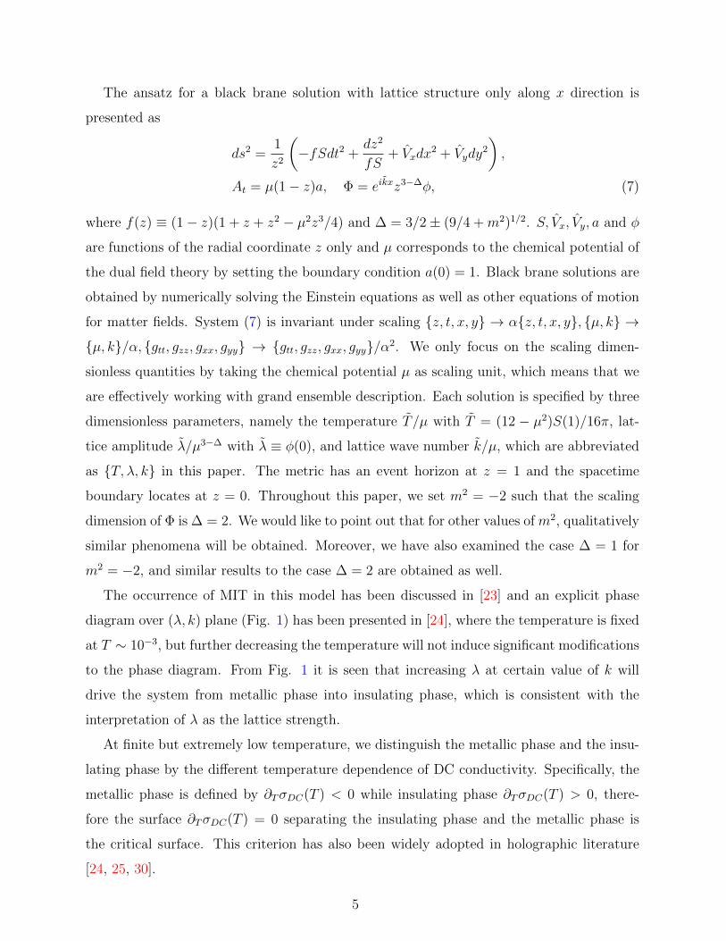
The ansatz for a black brane solution with lattice structure only along x direction is

presented as

ds2 =1

z2

(−fSdt2 +

dz2

fS+ Vxdx

2 + Vydy2

),

At = µ(1− z)a, Φ = eikxz3−∆φ, (7)

where f(z) ≡ (1− z)(1 + z + z2 − µ2z3/4) and ∆ = 3/2± (9/4 +m2)1/2. S, Vx, Vy, a and φ

are functions of the radial coordinate z only and µ corresponds to the chemical potential of

the dual field theory by setting the boundary condition a(0) = 1. Black brane solutions are

obtained by numerically solving the Einstein equations as well as other equations of motion

for matter fields. System (7) is invariant under scaling {z, t, x, y} → α{z, t, x, y}, {µ, k} →

{µ, k}/α, {gtt, gzz, gxx, gyy} → {gtt, gzz, gxx, gyy}/α2. We only focus on the scaling dimen-

sionless quantities by taking the chemical potential µ as scaling unit, which means that we

are effectively working with grand ensemble description. Each solution is specified by three

dimensionless parameters, namely the temperature T /µ with T = (12 − µ2)S(1)/16π, lat-

tice amplitude λ/µ3−∆ with λ ≡ φ(0), and lattice wave number k/µ, which are abbreviated

as {T, λ, k} in this paper. The metric has an event horizon at z = 1 and the spacetime

boundary locates at z = 0. Throughout this paper, we set m2 = −2 such that the scaling

dimension of Φ is ∆ = 2. We would like to point out that for other values of m2, qualitatively

similar phenomena will be obtained. Moreover, we have also examined the case ∆ = 1 for

m2 = −2, and similar results to the case ∆ = 2 are obtained as well.

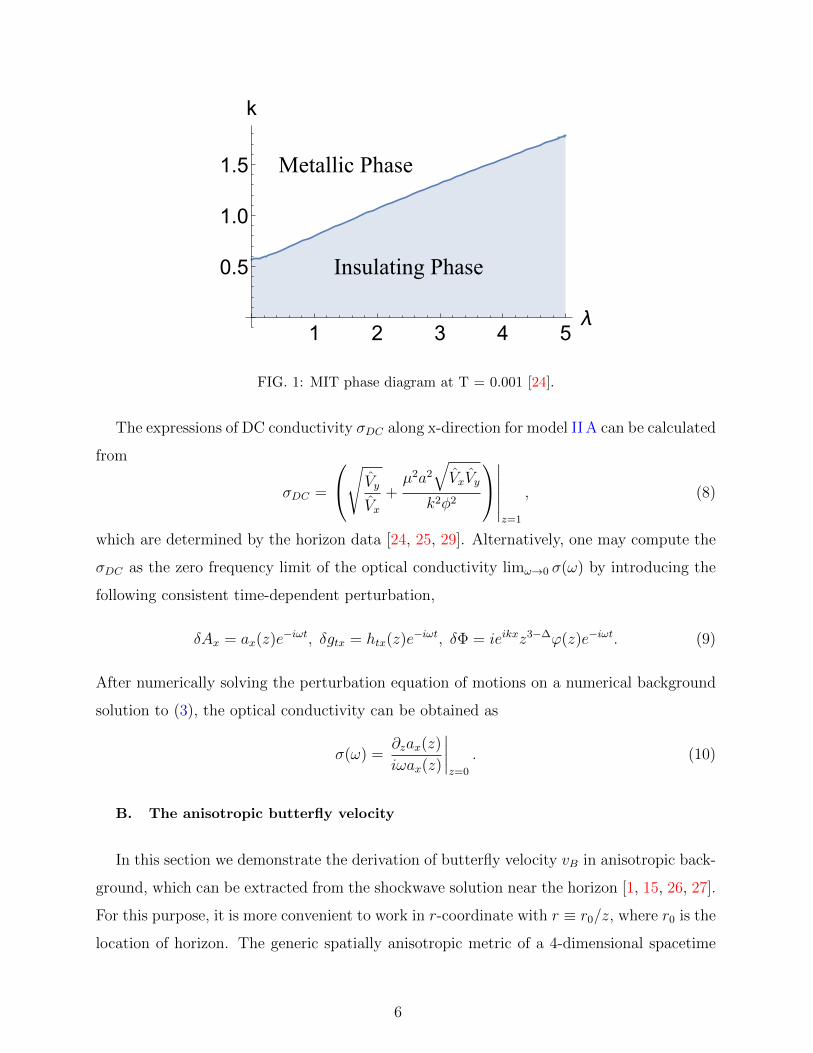
The occurrence of MIT in this model has been discussed in [23] and an explicit phase

diagram over (λ, k) plane (Fig. 1) has been presented in [24], where the temperature is fixed

at T ∼ 10−3, but further decreasing the temperature will not induce significant modifications

to the phase diagram. From Fig. 1 it is seen that increasing λ at certain value of k will

drive the system from metallic phase into insulating phase, which is consistent with the

interpretation of λ as the lattice strength.

At finite but extremely low temperature, we distinguish the metallic phase and the insu-

lating phase by the different temperature dependence of DC conductivity. Specifically, the

metallic phase is defined by ∂TσDC(T ) < 0 while insulating phase ∂TσDC(T ) > 0, there-

fore the surface ∂TσDC(T ) = 0 separating the insulating phase and the metallic phase is

the critical surface. This criterion has also been widely adopted in holographic literature

[24, 25, 30].

5

1 2 3 4 5λ

0.5

1.0

1.5

k

Insulating Phase

Metallic Phase

FIG. 1: MIT phase diagram at T = 0.001 [24].

The expressions of DC conductivity σDC along x-direction for model II A can be calculated

from

σDC =

√ Vy

Vx+µ2a2

√VxVy

k2φ2

∣∣∣∣∣∣z=1

, (8)

which are determined by the horizon data [24, 25, 29]. Alternatively, one may compute the

σDC as the zero frequency limit of the optical conductivity limω→0 σ(ω) by introducing the

following consistent time-dependent perturbation,

δAx = ax(z)e−iωt, δgtx = htx(z)e−iωt, δΦ = ieikxz3−∆ϕ(z)e−iωt. (9)

After numerically solving the perturbation equation of motions on a numerical background

solution to (3), the optical conductivity can be obtained as

σ(ω) =∂zax(z)

iωax(z)

∣∣∣∣z=0

. (10)

B. The anisotropic butterfly velocity

In this section we demonstrate the derivation of butterfly velocity vB in anisotropic back-

ground, which can be extracted from the shockwave solution near the horizon [1, 15, 26, 27].

For this purpose, it is more convenient to work in r-coordinate with r ≡ r0/z, where r0 is the

location of horizon. The generic spatially anisotropic metric of a 4-dimensional spacetime

6

can be written as

ds2 = −U(r)dt2 +dr2

U(r)+ Vx(r)dx

2 + Vy(r)dy2. (11)

In Kruskal coordinate (11) is written as

ds2 = U(uv)dudv + Vx(uv)dx2 + Vy(uv)dy2, (12)

where uv = −eU ′(r0)r∗(r), u/v = −e−U ′(r0)t, with r∗ being the tortoise coordinate defined

by dr∗ = dr/U(r). In addition, U(uv) = 4U(r)uvU ′(r0)2

, Vx,y(uv) = Vx,y(r). Note that, in this

coordinate the horizon is at u = v = 0.

The shockwave geometry is induced by a freely falling particle on the AdS boundary

at ti in the past and at x = y = 0. This particle is exponentially accelerated in Kruskal

coordinate and generates the following energy distribution at u = 0,

δTuu ∼ E0e2πβtiδ(u)δ(x, y), (13)

where E0 is the initial asymptotic energy of the particle. After the scrambling time t∗ ∼

β logN2 an initially small perturbation becomes significant and back-react to the geometry

by a shockwave localized at the horizon [31],

ds2 =Vx(uv)dx2 + Vy(uv)dy2 + U(uv)dudv

− U(uv)δ(u)h(x, y)du2.(14)

By a convenient redefinition y ≡ y√

Vx(0)Vy(0)

the resultant Einstein equation can be written as

a Poisson equation,(∂2x + ∂2

y −m2)h(x, y) ∼ 16πGNVx(0)

U(0)E0e

2πβtiδ(x, y), (15)

with m2 given by

m2 =4

U(uv)

(V ′x(uv) +

Vx(uv)V ′y(uv)

Vy(uv)

)∣∣∣∣u=0

. (16)

At long distance |~x| ≡√x2 + y2 > m−1, the solution reads as

h(x, y) ∼ E0e2πβ

(ti−t∗)−m|~x|

|~x|1/2. (17)

From (17) we read off the Lyapunov exponent λL and the butterfly velocity vB,

λL =2π

β, vB =

2π

βm(18)

7

The Lyapunov exponent saturates the chaos bound as expected. Rewriting m in coordinates

(r, t, x, y) we find

vB =

√πTVy(r0)

V ′x(r0)Vy(r0) + Vx(r0)V ′y(r0). (19)

When recovered to (x, y) coordinate system, the butterfly velocity vB is anisotropic. Specif-

ically, in direction with polar angle θ,

vB(θ) = vB

√sec2(θ)Vx (r0)

Vx (r0) + tan2(θ)Vy (r0). (20)

C. Evidences from holographic theories

In this subsection we explicitly study the relation between the QPT and the butterfly

velocity in Q-lattice model. We approach the QPT by studying the phase transitions in

zero temperature limit. Therefore, our main task is to investigate the butterfly velocity

on background solutions specified by (λ, k), which correspond to lattice strength and wave

number, respectively. For simplicity, we focus on λ = 2 and study the behavior of the but-

terfly velocity along x-direction, i.e., vB over k in low temperature region 2. The anisotropy

of the butterfly velocity will be addressed in the next subsection.

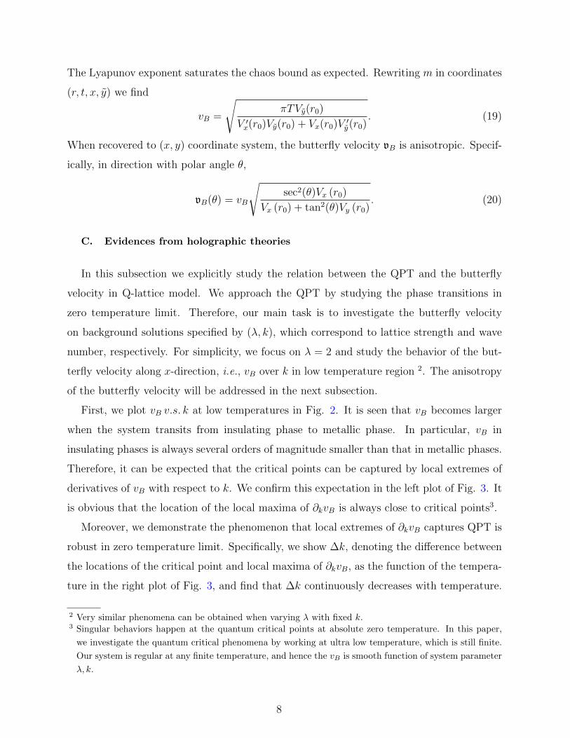
First, we plot vB v.s. k at low temperatures in Fig. 2. It is seen that vB becomes larger

when the system transits from insulating phase to metallic phase. In particular, vB in

insulating phases is always several orders of magnitude smaller than that in metallic phases.

Therefore, it can be expected that the critical points can be captured by local extremes of

derivatives of vB with respect to k. We confirm this expectation in the left plot of Fig. 3. It

is obvious that the location of the local maxima of ∂kvB is always close to critical points3.

Moreover, we demonstrate the phenomenon that local extremes of ∂kvB captures QPT is

robust in zero temperature limit. Specifically, we show ∆k, denoting the difference between

the locations of the critical point and local maxima of ∂kvB, as the function of the tempera-

ture in the right plot of Fig. 3, and find that ∆k continuously decreases with temperature.

2 Very similar phenomena can be obtained when varying λ with fixed k.3 Singular behaviors happen at the quantum critical points at absolute zero temperature. In this paper,

we investigate the quantum critical phenomena by working at ultra low temperature, which is still finite.

Our system is regular at any finite temperature, and hence the vB is smooth function of system parameter

λ, k.

8

1.08 1.12 1.16k

3.0

3.5

4.0

4.5

5.0

vB(10-3)T = 10-4

1.08 1.12 1.16k

2

4

6

8

10

vB(10-4)T = 10-5

1.08 1.12 1.16k

1

2

3

4

5

6

7

vB(10-7)T = 10-9

1.08 1.12 1.16k

5

10

15

20

25

vB(10-9)T = 10-11

FIG. 2: vB v.s. k at different low temperatures T = 10−4, 10−5, 10−9, 10−11 respectively. In each

plot the dotted line in red represents the location of QCP, separating the insulating phase (left

side) and metallic phase (right side).

1.08 1.10 1.12 1.14 1.16k

1

2

3

4

5

6

7∂kvB(10-7)

λ=2, T=10-11

10-410-510-610-710-810-910-1010-11T

0.005

0.010

0.015

Δk

FIG. 3: The left plot is ∂kvB v.s. k at T = 10−11, in which the red vertical line represents the

position of the critical point while the blue line denotes the position of the local maximum of ∂kvB.

The right plot is for the temperature dependence of ∆k.

Therefore we arrive at the conclusion that in Q-lattice model II A the local extreme of ∂kvB

can be used to characterize the QPT in zero temperature limit.

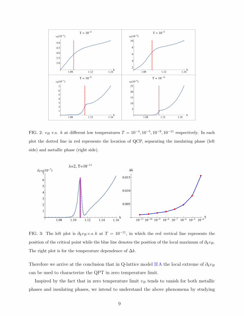
Inspired by the fact that in zero temperature limit vB tends to vanish for both metallic

phases and insulating phases, we intend to understand the above phenomena by studying

9

k=0.500

k=0.805

k=1.31

k=1.50

10-9 10-7 10-5 0.001 0.100T

0.2

0.4

0.6

0.8

1.0

1.2

Tv'B/vB

λ=2

Tv'B/vB=0.5

FIG. 4: Tv′B/vB v.s. T for different phases (k = 0.500, 0.805 corresponds to metallic phases and

k = 1.31, 1.50 corresponds to insulating phases). The purple dashed line points to Tv′B/vB = 0.5.

the scaling of vB with temperature vB ∼ Tα in both metallic and insulating phases. Fig. 4

demonstrates Tv′B/vB as a function of T , which captures the exponent α in different phases.

One finds α = 1/2 for metallic phases in low temperature region. This originates from

the fact that metallic phases in Q-lattice model II A always correspond to the well-known

AdS2 × R2 IR geometry, on which vB ∼ T 1/2 can be deduced [16]. While for insulating

phases, Tv′B/vB tends to converge to a fixed value close to 1 down to ultra low temperature

T = 10−11, which implies that the insulating phases for model II A may correspond to a

single IR geometry different from AdS2 × R2 4. Therefore we conclude that vB scaling

distinctly with temperature in metallic phases and insulating phases, are responsible for the

rapid change of vB observed in Fig. 2, as well as the local extremes of ∂kvB near QCPs

observed in Fig. 3.

The above understanding is also applicable for some other holographic MIT model. To

this end, we demonstrate another holographic model [29], in which MIT is also achieved

when varying the system parameters in the region −1/3 < γ 6 −1/12, where γ is the

parameter of the action. Like model II A, we obtain vB ∼ T 1/2 in metallic phases again, due

to the AdS2 × R2 IR geometry. While for insulating phases we find α = 2γ2+7γ+212γ2+4γ+18

, which

4 However, we would like to point out that the exact IR fixed point of Q-lattice model is unknown so far

[23].

10

k=1.052

k=1.077

k=1.086

k=1.096

π

4π

2

θ

-24

-23

-22

-21

Log[B(θ)]λ=2, T=10-11

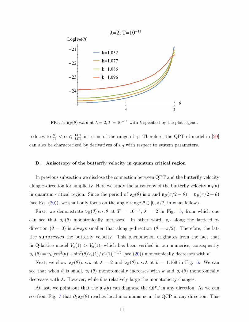
FIG. 5: vB(θ) v.s. θ at λ = 2, T = 10−11 with k specified by the plot legend.

reduces to 8576< α 6 1471

1273in terms of the range of γ. Therefore, the QPT of model in [29]

can also be characterized by derivatives of vB with respect to system parameters.

D. Anisotropy of the butterfly velocity in quantum critical region

In previous subsection we disclose the connection between QPT and the butterfly velocity

along x-direction for simplicity. Here we study the anisotropy of the butterfly velocity vB(θ)

in quantum critical region. Since the period of vB(θ) is π and vB(π/2 − θ) = vB(π/2 + θ)

(see Eq. (20)), we shall only focus on the angle range θ ∈ [0, π/2] in what follows.

First, we demonstrate vB(θ) v.s. θ at T = 10−11, λ = 2 in Fig. 5, from which one

can see that vB(θ) monotonically increases. In other word, vB along the latticed x-

direction (θ = 0) is always smaller that along y-direction (θ = π/2). Therefore, the lat-

tice suppresses the butterfly velocity. This phenomenon originates from the fact that

in Q-lattice model Vx(1) > Vy(1), which has been verified in our numerics, consequently

vB(θ) = vB[cos2(θ) + sin2(θ)Vy(1)/Vx(1)]−1/2 (see (20)) monotonically decreases with θ.

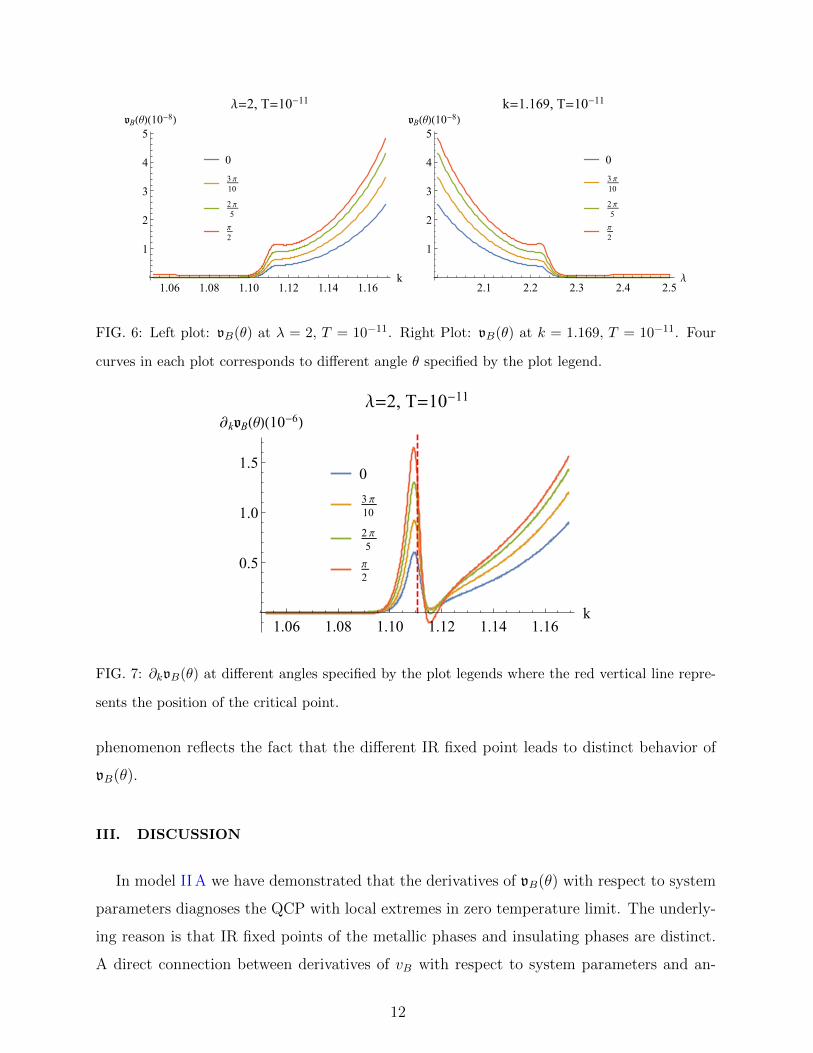
Next, we show vB(θ) v.s. k at λ = 2 and vB(θ) v.s. λ at k = 1.169 in Fig. 6. We can

see that when θ is small, vB(θ) monotonically increases with k and vB(θ) monotonically

decreases with λ. However, while θ is relatively large the monotonicity changes.

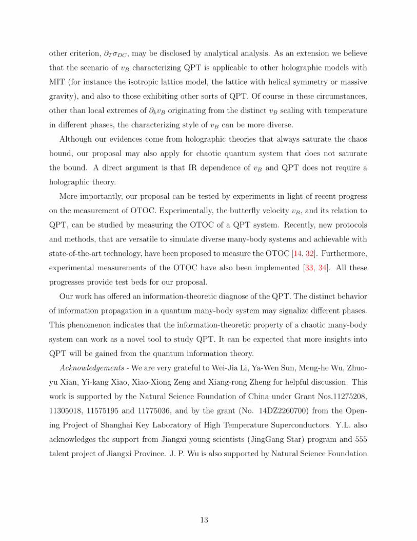
At last, we point out that the vB(θ) can diagnose the QPT in any direction. As we can

see from Fig. 7 that ∂kvB(θ) reaches local maximums near the QCP in any direction. This

11

0

3 π10

2 π5

π

2

1.06 1.08 1.10 1.12 1.14 1.16k

1

2

3

4

5B(θ)(10-8)

λ=2, T=10-11

0

3 π10

2 π5

π

2

2.1 2.2 2.3 2.4 2.5λ

1

2

3

4

5B(θ)(10-8)

k=1.169, T=10-11

FIG. 6: Left plot: vB(θ) at λ = 2, T = 10−11. Right Plot: vB(θ) at k = 1.169, T = 10−11. Four

curves in each plot corresponds to different angle θ specified by the plot legend.

0

3 π10

2 π5

π

2

1.06 1.08 1.10 1.12 1.14 1.16k

0.5

1.0

1.5

∂kB(θ)(10-6)λ=2, T=10-11

FIG. 7: ∂kvB(θ) at different angles specified by the plot legends where the red vertical line repre-

sents the position of the critical point.

phenomenon reflects the fact that the different IR fixed point leads to distinct behavior of

vB(θ).

III. DISCUSSION

In model II A we have demonstrated that the derivatives of vB(θ) with respect to system

parameters diagnoses the QCP with local extremes in zero temperature limit. The underly-

ing reason is that IR fixed points of the metallic phases and insulating phases are distinct.

A direct connection between derivatives of vB with respect to system parameters and an-

12

other criterion, ∂TσDC , may be disclosed by analytical analysis. As an extension we believe

that the scenario of vB characterizing QPT is applicable to other holographic models with

MIT (for instance the isotropic lattice model, the lattice with helical symmetry or massive

gravity), and also to those exhibiting other sorts of QPT. Of course in these circumstances,

other than local extremes of ∂kvB originating from the distinct vB scaling with temperature

in different phases, the characterizing style of vB can be more diverse.

Although our evidences come from holographic theories that always saturate the chaos

bound, our proposal may also apply for chaotic quantum system that does not saturate

the bound. A direct argument is that IR dependence of vB and QPT does not require a

holographic theory.

More importantly, our proposal can be tested by experiments in light of recent progress

on the measurement of OTOC. Experimentally, the butterfly velocity vB, and its relation to

QPT, can be studied by measuring the OTOC of a QPT system. Recently, new protocols

and methods, that are versatile to simulate diverse many-body systems and achievable with

state-of-the-art technology, have been proposed to measure the OTOC [14, 32]. Furthermore,

experimental measurements of the OTOC have also been implemented [33, 34]. All these

progresses provide test beds for our proposal.

Our work has offered an information-theoretic diagnose of the QPT. The distinct behavior

of information propagation in a quantum many-body system may signalize different phases.

This phenomenon indicates that the information-theoretic property of a chaotic many-body

system can work as a novel tool to study QPT. It can be expected that more insights into

QPT will be gained from the quantum information theory.

Acknowledgements - We are very grateful to Wei-Jia Li, Ya-Wen Sun, Meng-he Wu, Zhuo-

yu Xian, Yi-kang Xiao, Xiao-Xiong Zeng and Xiang-rong Zheng for helpful discussion. This

work is supported by the Natural Science Foundation of China under Grant Nos.11275208,

11305018, 11575195 and 11775036, and by the grant (No. 14DZ2260700) from the Open-

ing Project of Shanghai Key Laboratory of High Temperature Superconductors. Y.L. also

acknowledges the support from Jiangxi young scientists (JingGang Star) program and 555

talent project of Jiangxi Province. J. P. Wu is also supported by Natural Science Foundation

13

of Liaoning Province under Grant Nos.201602013.

[1] D. A. Roberts and B. Swingle, Phys. Rev. Lett. 117, no. 9, 091602 (2016) [arXiv:1603.09298

[hep-th]].

[2] J. M. Maldacena, Adv. Theor. Math. Phys. 2 (1998) 231, [arXiv:hep-th/9711200].

[3] E. Witten, Adv. Theor. Math. Phys. (1998) 253, [arXiv:hep-th/9802150].

[4] A. Donos and S. A. Hartnoll, Nature Phys. 9, 649 (2013) [arXiv:1212.2998].

[5] S. H. Shenker and D. Stanford, JHEP 1403, 067 (2014) [arXiv:1306.0622 [hep-th]].

[6] S. H. Shenker and D. Stanford, JHEP 1412, 046 (2014) [arXiv:1312.3296 [hep-th]].

[7] D. A. Roberts, D. Stanford and L. Susskind, “Localized shocks,” JHEP 1503, 051 (2015)

[arXiv:1409.8180 [hep-th]].

[8] D. A. Roberts and D. Stanford, Phys. Rev. Lett. 115, no. 13, 131603 (2015) [arXiv:1412.5123

[hep-th]].

[9] S. H. Shenker and D. Stanford, JHEP 1505, 132 (2015) [arXiv:1412.6087 [hep-th]].

[10] J. Maldacena, S. H. Shenker and D. Stanford, JHEP 1608, 106 (2016) [arXiv:1503.01409

[hep-th]].

[11] J. Polchinski, “Chaos in the black hole S-matrix,” arXiv:1505.08108 [hep-th].

[12] P. Hosur, X. L. Qi, D. A. Roberts and B. Yoshida, JHEP 1602 (2016) 004 [arXiv:1511.04021

[hep-th]].

[13] J. Polchinski and V. Rosenhaus, “The Spectrum in the Sachdev-Ye-Kitaev Model,” JHEP

1604, 001 (2016) [arXiv:1601.06768 [hep-th]].

[14] B. Swingle, G. Bentsen, M. Schleier-Smith and P. Hayden, arXiv:1602.06271 [quant-ph].

[15] M. Blake, “Universal Charge Diffusion and the Butterfly Effect,” arXiv:1603.08510 [hep-th].

[16] M. Blake, “Universal Diffusion in Incoherent Black Holes,” arXiv:1604.01754 [hep-th].

[17] A. Lucas and J. Steinberg, “Charge diffusion and the butterfly effect in striped holographic

matter,” arXiv:1608.03286 [hep-th].

[18] A. Kitaev, “Hidden correlations in the hawking radiation and thermal noise,” (2014), talk

given at the Fundamental Physics Prize Symposium, Nov. 10, 2014.

[19] S. A. Hartnoll, “Theory of universal incoherent metallic transport,” Nature Phys. 11, 54

(2015) [arXiv:1405.3651 [cond-mat.str-el]].

14

[20] H. Shen, P. Zhang, R. Fan and H. Zhai, arXiv:1608.02438 [cond-mat.str-el].

[21] R. Fan, P. Zhang, H. Shen and H. Zhai, arXiv:1608.01914 [cond-mat.str-el].

[22] J. M. Deutsch, Phys. Rev. A 43, 2146 (1991).

[23] A. Donos and J. P. Gauntlett, JHEP 1404, 040 (2014) [arXiv:1311.3292 [hep-th]].

[24] Y. Ling, P. Liu, C. Niu, J. P. Wu and Z. Y. Xian, JHEP 1604, 114 (2016) [arXiv:1502.03661

[hep-th]].

[25] Y. Ling, P. Liu and J. P. Wu, Phys. Rev. D 93, no. 12, 126004 (2016) [arXiv:1604.04857

[hep-th]].

[26] T. Dray and G. ’t Hooft, Nucl. Phys. B 253, 173 (1985).

[27] Y. Kiem, H. L. Verlinde and E. P. Verlinde, Phys. Rev. D 52, 7053 (1995) [hep-th/9502074].

[28] R. G. Cai, X. X. Zeng and H. Q. Zhang, JHEP 1707, 082 (2017)

doi:10.1007/JHEP07(2017)082 [arXiv:1704.03989 [hep-th]].

[29] A. Donos and J. P. Gauntlett, JHEP 1406, 007 (2014) [arXiv:1401.5077 [hep-th]].

[30] M. Baggioli and O. Pujolas, Phys. Rev. Lett. 114, no. 25, 251602 (2015) [arXiv:1411.1003

[hep-th]].

[31] Y. Sekino and L. Susskind, JHEP 0810, 065 (2008) [arXiv:0808.2096 [hep-th]].

[32] N. Y. Yao, F. Grusdt, B. Swingle, M. D. Lukin, D. M. Stamper-Kurn, J. E. Moore and

E. A. Demler, arXiv:1607.01801 [quant-ph].

[33] M. Garttner, J. G. Bohnet, A. Safavi-Naini, M. L. Wall, J. J. Bollinger and A. M. Rey,

arXiv:1608.08938 [quant-ph].

[34] J. Li, R. H. Fan, H. Y. Wang, B. T. Ye, B. Zeng, H. Zhai, X. H. Peng and J. F. Du,

arXiv:1609.01246 [cond-mat.str-el]

15