department of mines and petroleum · dynamic modelling of co 2 sequestration in the harvey area a...

Dynamic Modelling of CO2 Sequestration

In the

Harvey Area

A Report by ODIN Reservoir Consultants

For

Department of Mines and Petroleum

DMP/2016/5

July 2016

DMP Confidential

of 65 July 2016

LIST OF FIGURES .................................................................................................................................. 3

LIST OF TABLES .................................................................................................................................... 4

DECLARATION ....................................................................................................................................... 5

NOTE: ...................................................................................................................................................... 5

1. EXECUTIVE SUMMARY ................................................................................................................. 6

2. INTRODUCTION .............................................................................................................................. 7

3. INPUT DATA .................................................................................................................................... 8

3.1 TEMPERATURE REGIME ............................................................................................................... 8 3.2 PRESSURE REGIME ..................................................................................................................... 9 3.3 FLUID FLOW PROPERTIES .......................................................................................................... 10

3.3.1 CO2 relative Permeability and Trapped Gas Saturation (SgT) ......................................... 11 3.3.1.1 Trapped Gas Saturation (SgT) .................................................................................................................... 11

3.4 WATER RELATIVE PERMEABILITY ................................................................................................ 13 3.4.1 CO2 Relative Permeability ............................................................................................... 14

3.5 BRINE SALINITY ......................................................................................................................... 14 3.6 GEOMECHANICS ........................................................................................................................ 15 3.7 GEOLOGICAL MODEL ................................................................................................................. 19

4. UPSCALING .................................................................................................................................. 20

4.1 DESCRIPTION OF THE SECTOR MODELS ...................................................................................... 21 4.1.1 Model Run Parameters .................................................................................................... 22

4.2 MODEL RESULTS ....................................................................................................................... 25 4.2.1 Yalgorup ........................................................................................................................... 25 4.2.2 Wonnerup ........................................................................................................................ 26

5. INJECTIVITY STUDIES ................................................................................................................. 29

5.1 REFERENCE CASE ..................................................................................................................... 29 5.2 IMPACT OF RESERVOIR UNCERTAINTIES ..................................................................................... 30

6. MODELLING OF THE CO2 PLUME .............................................................................................. 34

6.1 SIMULATOR SELECTION ............................................................................................................. 34 6.2 MODEL DESCRIPTION ................................................................................................................ 34 6.3 INITIALISATION PARAMETERS ...................................................................................................... 36 6.4 PVT MODEL .............................................................................................................................. 37 6.5 AQUIFER EXTENT ...................................................................................................................... 37 6.6 RESERVOIR PROPERTIES ........................................................................................................... 38 6.7 CONCEPTUAL DEVELOPMENT PLAN – REFERENCE CASE ............................................................. 40

6.7.1 Reference Case Definition ............................................................................................... 40 6.7.2 Results ............................................................................................................................. 41

6.8 IMPACT OF RESERVOIR UNCERTAINTIES ON THE MOVEMENT OF THE CO2 PLUME .......................... 45 6.8.1 Case 1 – High Vertical Permeability (“Holey Faults”) ...................................................... 45 6.8.2 Case 2 – High Gas Relative Permeability (krg=0.23) ...................................................... 47 6.8.3 Case 3 – Low Trapped Gas Saturation (SgT=0.10) ......................................................... 49 6.8.4 Case 4 - High Permeability Case ..................................................................................... 50 6.8.5 Case 5 – High kv/kh (Vertical to Horizontal Permeability Ratio)...................................... 52 6.8.6 Case 6 – Deterministic Scenario ..................................................................................... 53 6.8.7 Case 7 – Faults transmissibility multiplied by 0.1 ............................................................ 56 6.8.8 Case 8 – Low CO2 Solubility ............................................................................................ 57

7. STRESS SCENARIOS ................................................................................................................... 60

7.1 CASE 9 - HIGH RATE .................................................................................................................. 60 7.2 CASE 10 – LOW SOLUBILITY AND LOW TRAPPED GAS SATURATION ............................................. 62

8. FURTHER WORK .......................................................................................................................... 64

DMP Confidential

of 65 July 2016

9. REFERENCES ............................................................................................................................... 65

List of Figures

Figure 1 Location Map of the Harvey Area showing the Area of Interest............................. 7 Figure 2 Temperature Measurements for the Harvey wells ................................................. 8 Figure 3 Pressure data from RCI tool run in Harvey-1 and Harvey-4 .................................. 9 Figure 4 Steady-state imbibition data (Sample 20) – Harvey-3 ......................................... 12 Figure 5 Water Relative Permeability Data (Harvey-1 and Harvey-3) ............................... 13 Figure 6 Drainage and Imbibition Water Relative Permeability (Sample 20 Harvey-3) ..... 14 Figure 7 Geomechanical Model A - Yalgorup .................................................................... 16 Figure 8 Geomechanical Model B - Yalgorup .................................................................... 17 Figure 9 Geomechanical Model C – Yalgorup ................................................................... 17 Figure 10 Geomechanical Model A - Wonnerup ................................................................ 18 Figure 11 Geomechanical Model B - Wonnerup ................................................................ 18 Figure 12 Geomechanical Model C - Wonnerup ................................................................ 19 Figure 13 View of the Petrel Model of the Area of Interest in the Harvey Area ................. 20 Figure 14 View of the Petrel Model showing the area selected for the Sector model. ....... 21 Figure 15 Sector Model of the Yalgorup and Wonnerup .................................................... 23 Figure 16 Sector Model Showing Pore Volume Multipliers ................................................ 24 Figure 17 Reference Case Relative Permeability Curves .................................................. 24 Figure 18 Bottom hole pressure Response - Yalgorup Model ........................................... 26 Figure 19 Gas Saturation Distribution – Yalgorup .............................................................. 26 Figure 20 Bottom hole pressure Response - Wonnerup Model ......................................... 27 Figure 21 Gas Saturation Distribution – Wonnerup (Comparison of 1 and 2 m models) ... 27 Figure 22 Gas Saturation Distribution – Wonnerup (Comparison of 1 and 4 m models) ... 28 Figure 23 Reference Case Model – Injection Performance (Single Well Model) ............... 30 Figure 24 Tornado Chart Showing Impact of Reservoir Uncertainties on Injectivity .......... 32 Figure 25 Probability Distribution of Injectivity Over 30 Years ........................................... 33 Figure 26 Coarse Scale Model Showing Porosity Distribution ........................................... 35 Figure 27 Comparison of Permeability Distribution - Fine and Coarse Scale Models ....... 36 Figure 28 Connected Body Analysis - Fine and Coarse Scale Models .............................. 36 Figure 29 Time Structure maps of the: a) top Yalgorup Member; b) top Wonnerup Member (After

Reference 7) ................................................................................................................ 37 Figure 30 Modelling the Extent of the Wonnerup and Yalgorup Aquifers .......................... 38 Figure 31 X-Section through the Harvey Full Field Model – Horizontal Permeability ........ 39 Figure 32 X-Section through the Harvey Full Field Model – Vertical Permeability ............ 39 Figure 33 X-Section through the Harvey Full Field Model – Porosity ................................ 40 Figure 34 Injection Performance – Reference Case .......................................................... 42 Figure 35 Bottom Hole Pressure Profile by Well During Injection – Reference Case ........ 43 Figure 36 Top View – Reference Case CO2 Distribution at end of Injection Period .......... 43 Figure 37 Top View – Reference Case CO2 Distribution 1000 years after injection .......... 44 Figure 38 Reference Case – X-Section through HI-2 and HI-6 .......................................... 44 Figure 39 X-Section (I=35) through the model showing high permeability conduits .......... 46 Figure 40 Top View – CO2 Distribution (Comparison of Reference Case and Case 1) ..... 46 Figure 41 X-Section View – CO2 Distribution (Comparison of Reference Case and Case 1)47 Figure 42 Gas Relative Permeability (Comparison of Reference Case and Case 2) ........ 48 Figure 43 Top View – CO2 Distribution (Comparison of Reference Case and Case 2) ..... 48 Figure 44 X-Section View – CO2 Distribution (Case 2) ...................................................... 49 Figure 45 Top View – CO2 Distribution (Comparison of Reference Case and Case 3) ..... 50 Figure 46 X-Section View – CO2 Distribution (Case 3) ...................................................... 50 Figure 47 Top View – CO2 Distribution (Comparison of Reference Case and Case 4) ..... 51 Figure 48 X-Section View – CO2 Distribution (Case 4) ...................................................... 51 Figure 49 Top View – CO2 Distribution (Comparison of Reference Case and Case 5) ..... 52 Figure 50 X-Section View – CO2 Distribution (Case 5) ...................................................... 53 Figure 51 Harvey-1 – Gamma ray and interpreted porosity log. ........................................ 54

DMP Confidential

of 65 July 2016

Figure 52 Top View – CO2 Distribution (Comparison of Reference Case and Case 6) ..... 55 Figure 53 X-Section View – CO2 Distribution (Case 6) ...................................................... 55 Figure 54 Top View – CO2 Distribution (Comparison of Reference Case and Case 7) ..... 56 Figure 55 X-Section View – CO2 Distribution (Case 7) ...................................................... 57 Figure 56 CO2 Solubility in Brine (500 years after Cessation of Injection) ......................... 58 Figure 57 Top View – CO2 Distribution (Comparison of Reference Case and Case 8) ..... 58 Figure 58 X-Section View – CO2 Distribution (Case 8) ...................................................... 59 Figure 59 Injection Performance –Case 9 .......................................................................... 61 Figure 60 Bottom Hole Pressure Profile by Well During Injection – High Rate Case ........ 61 Figure 61 Top View - CO2 Distribution (Reference Case and Case 9) .............................. 62 Figure 62 X-Section View – CO2 Distribution (Case 9) ...................................................... 62 Figure 63 Top View - CO2 Distribution (Reference Case and Case 10) ............................ 63 Figure 64 X-Section View – CO2 Distribution (Case 10) .................................................... 63 List of Tables Table 1 Special Core Analysis sample Distribution (Harvey-1, -3 and -4) ......................... 10 Table 2 Primary Drainage and Primary Imbibition (CSIRO data – Reference 1) ............... 11 Table 3 Water Displacing CO2 - Sample 20 (Harvey-3) .................................................... 12 Table 4 Brine Samples from Harvey ................................................................................... 15 Table 5 Impact of Reservoir Uncertainties on Injectivity in the Wonnerup ......................... 31 Table 6 Range of Gas injected – Combined Uncertainties ................................................ 33 Table 7 Material Balance Accounting (1000 Years after Injection) .................................... 45 Table 8 Case Summary – Full Field Model of the Harvey Area ......................................... 45 Table 9 Summary Table for Stress Scenarios .................................................................... 60

DMP Confidential

of 65 July 2016

Declaration

ODIN Reservoir Consultants has been commissioned to undertake to provide a reservoir modelling study for the South West Hub CO2 Sequestration Project on behalf of The Department of Minerals and Petroleum, (DMP) The evaluation of Carbon Capture and Storage is subject to uncertainty because it involves judgments on many variables that cannot be precisely assessed, including CO2 sequestration rates and capture, the costs associated with storing these volumes, sequestration gas distribution and potential impact of fiscal/regulatory changes. The statements and opinions attributable to us are given in good faith and in the belief that such statements are neither false nor misleading. In carrying out our tasks, we have considered and relied upon information supplied by the DMP and available in the public domain. Whilst every effort has been made to verify data and resolve apparent inconsistencies, neither ODIN Reservoir Consultants nor its servants accept any liability for its accuracy, nor do we warrant that our enquiries have revealed all of the matters, which an extensive examination should disclose. We believe our review and conclusions are sound but no warranty of accuracy or reliability is given to our conclusions. Neither ODIN Reservoir Consultants nor its employees has any pecuniary interest or other interest in the assets evaluated other than to the extent of the professional fees receivable for the preparation of this report Note: ODIN has conducted the attached independent technical evaluation with the following internationally recognised specialists: David Lim is a member of the Society of Petroleum Engineers (SPE). He has over 30 years of international reservoir engineering experience in Europe, North and South America, North and West Africa, Middle East, Asia and Australasia. David is an internationally recognised reservoir simulation and reservoir engineering expert and has specialist expertise in field development planning, reservoir engineering, reserves reviews and simulation. David has been the Reservoir Simulation and Reservoir Engineering Advisor to NOCs, major and independent operators in Australia and SE Asia. David has also chaired SPE committees and forums on reservoir simulation, well testing and field development planning.

DMP Confidential

of 65 July 2016

1. EXECUTIVE SUMMARY

ODIN Reservoir Consultants has been commissioned by the Department of Mines and

Petroleum (WA) to provide a multi-disciplinary group with sub-surface skill sets to:

1) Undertake an interpretation of the 3D seismic data;

2) provide support through reservoir model building and updating of the South West

Hub Project in the southern Perth Basin; and

3) provide on-going technical support.

As an integral part of the above, ODIN Reservoir Consultants conducted reservoir

simulation studies to assess the suitability of the Lesueur Sandstone in the Lower

Lesueur Region of Western Australia as a potential carbon dioxide geological

sequestration site..

The objective of the simulation study is to provide a suite of full field simulation models

which cover a range of subsurface uncertainties that provides confidence that the CO2

plume stays below 800 mTVDss and within the storage complex for 1000 years. The

results of this study will enable a Go/No Go decision on additional data acquisition in the

Harvey area.

The results of the modelling show that it could be feasible to inject 800,000 tpa of CO2

over 30 years in the Yalgorup and Wonnerup formations in the Harvey area. Our

modelling studies show that all of the injected CO2 remains in the Wonnerup and that the

main factors controlling CO2 plume migration are trapped gas saturation and the solubility

of CO2 in brine. Uncertainties in end point relative permeability, vertical permeability or

the fraction of high energy facies in the Wonnerup are a second order effect. The study

also highlights the lack of SCAL, steady state trapped gas saturation in particular, and

water salinity data from the Harvey area which can be used to further constrain the range

of results from the simulation studies.

ODIN also recommends that detailed fine grid simulations be conducted to examine the

impact of coarsening the grid in the lateral direction and also to calibrate the solubility of

CO2 in the coarse grid blocks.

DMP Confidential

of 65 July 2016

2. INTRODUCTION

ODIN Reservoir Consultants has been commissioned by the Department of Mines and

Petroleum (WA) to provide a multi-disciplinary group with sub-surface skill sets to:

1. Undertake an interpretation of the 3D seismic data;

2. provide support through reservoir model building and updating of the South West

Hub Project in the southern Perth Basin; and

3. provide on-going technical support.

As an integral part of the above, ODIN Reservoir Consultants conducted reservoir

simulation studies to assess the suitability of the Lesueur Sandstone in the Lower

Lesueur Region of Western Australia as a potential carbon dioxide geological

sequestration site capable of injecting 800,000 tonnes per annum of CO2 and containing

the CO2 for at least 1000 years of injection ceases.. The location and area of interest of

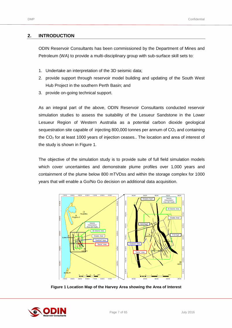
the study is shown in Figure 1.

The objective of the simulation study is to provide suite of full field simulation models

which cover uncertainties and demonstrate plume profiles over 1,000 years and

containment of the plume below 800 mTVDss and within the storage complex for 1000

years that will enable a Go/No Go decision on additional data acquisition.

Figure 1 Location Map of the Harvey Area showing the Area of Interest Page 3 Tel: +61-414-246-600

Location Map

Seismic

Interpretation

Area with Faults

3D Seismic Area

“GeoGrid” Area

“Sector” Area

Seismic

Interpretation

Area with Faults

3D Seismic Area

“Western Fault”

“F10 Fault”

“E-W Fault”

“GeoGrid” Area

“Sector” Area

“Greater Area”

“Greater Area”

DMP Confidential

of 65 July 2016

3. INPUT DATA

3.1 Temperature Regime

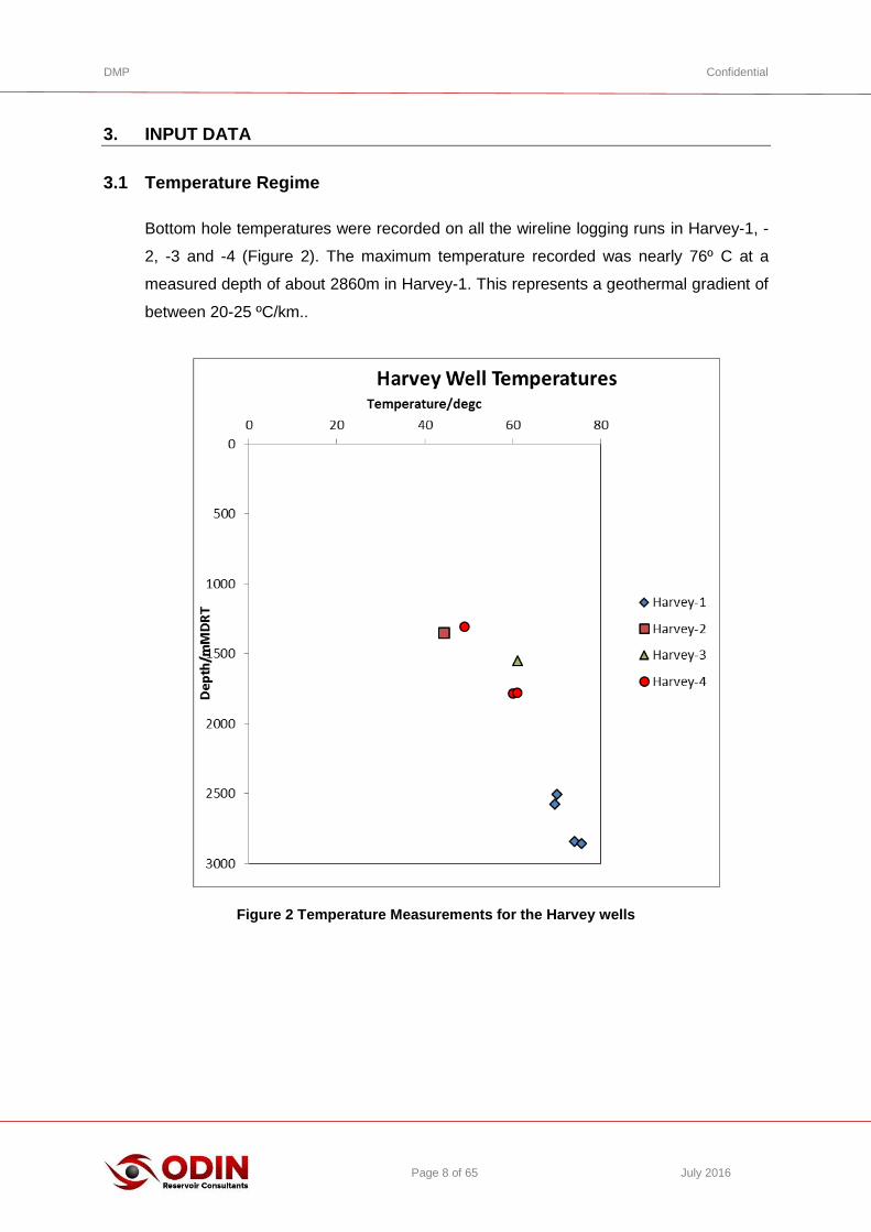
Bottom hole temperatures were recorded on all the wireline logging runs in Harvey-1, -

2, -3 and -4 (Figure 2). The maximum temperature recorded was nearly 76º C at a

measured depth of about 2860m in Harvey-1. This represents a geothermal gradient of

between 20-25 ºC/km..

Figure 2 Temperature Measurements for the Harvey wells

DMP Confidential

of 65 July 2016

3.2 Pressure Regime

Pressure measurements were made with the formation pressure sampling tools in

Harvey-1 and Harvey-4 are summarized in Figure 3. The data are consistent with a

normally pressured aquifer extending to surface.

Figure 3 Pressure data from RCI tool run in Harvey-1 and Harvey-4

y = 0.6888x - 1.8742

500

1000

1500

2000

2500

3000

500 1000 1500 2000 2500 3000 3500 4000

Dep

th (

mTV

Dss

)

Formation Pressure (psia)

Harvey-4

Harvey-1

DMP Confidential

of 65 July 2016

3.3 Fluid Flow Properties

Fluid flow properties on plugs from the Harvey cores were measured at in-situ reservoir

conditions (Reference 1 and 2). End point relative permeability data were measured for

eight samples from Harvey-3 (3 samples), Harvey-4 (2 samples) and Harvey-1 (3

samples). The plugs selected from the cores are from the two facies identified in the

Wonnerup: Low Energy (L-E Fluvial) and High Energy (H-E Fluvial).

The experiments on the Harvey-1 samples were conducted by CSIRO and the

experiments on the Harvey-3 and -4 samples were performed by Core Laboratories in

Houston. All of the CSIRO experiments were conducted on plugs from the H-E fluvial.

Table 1 summarises the results of the core experiments.

The plugs representing the H-E Fluvial facies from Harvey-3 and -4 failed during the

experiments. Steady state drainage and imbibition relative permeability curves were

obtained from Sample 20 from the Harvey-3 core.

Table 1 Special Core Analysis sample Distribution (Harvey-1, -3 and -4)

DMP Confidential

of 65 July 2016

3.3.1 CO2 relative Permeability and Trapped Gas Saturation (SgT)

3.3.1.1 Trapped Gas Saturation (SgT)

Unsteady state imbibition trapped gas saturations were measured on core plugs from

Harvey-1. The trapped gas saturations on these core plugs ranged from 23%-43% (Table

2). SgT from the unsteady state tests were not considered in this study as they were

unreliable as the imbibition curves were unavailable and the end point gas relative

permeability used to estimate the trapped gas saturation is unknown.

Table 2 Primary Drainage and Primary Imbibition (CSIRO data – Reference 1)

Core Laboratories conducted drainage and imbibition relative permeability experiments

on Sample 20 from Harvey-3 (Figure 4). Hysteresis in the CO2 relative permeability data

is evident and the reported SgT of 0.265 (Table 3) from the steady state experiments.

However, analysis of the data (Figure 4) shows that SgT was estimated from CO2 relative

permeability >0.001. In our opinion that is too optimistic for CO2 sequestration projects

where project time scales are in the hundreds of years. We recommend that the trapped

gas saturation, SgT, should be estimated with lower CO2 relative permeability. In our

study, we have selected the SgT of 0.19 at the minimum relative permeability of 0.00001.

In this study, the data from Core Laboratories was used to derive the trapped gas used

in the modelling as the data from CSIRO is incomplete.

Curtin

Samples

Primary Drainage

CO2 Displacing

Water

Primary Imbibition

Water Displacing

CO2

Primary Drainage

CO2 Displacing

Water

Primary Imbibition

Water Displacing

CO2

H-1 Final Sw Final Sg krg Krw

206647 45% 23% 0.22 0.35

206660 40% 43% 0.21 0.13

206669 42% 34% 0.17 0.10

DMP Confidential

of 65 July 2016

Table 3 Water Displacing CO2 - Sample 20 (Harvey-3)

Figure 4 Steady-state imbibition data (Sample 20) – Harvey-3

WATER - CO2 RELATIVE PERMEABILITY

Steady State Method Extracted State Samples

Net Confining Stress: 1700 psi Temperature: 118oF

PETROLEUM SERVICES

Company: Department of Mines and Petroleum

Well: Harvey-3

Location: Australia File: HOU-150878

Initial Conditions Terminal Conditions

Water Effective CO2 Effective Relative

Sample Klinkenberg Saturation, Permeability Saturation, Permeability Permeability CO2 Recovery,

Sample Depth, Permeability, Porosity, fraction to CO2, fraction to Water, to Water*, fraction fraction

Number meters millidarcies fraction pore space millidarcies pore space millidarcies fraction pore space gas-in-place

20 1429.00 17.6 0.220 0.492 0.792 0.265 0.467 0.110 0.243 0.479

* Relative to the Specific Permeability to Brine

0.00001

0.00010

0.00100

0.01000

0.10000

1.00000

0.00 0.10 0.20 0.30 0.40 0.50 0.60

CO

2 R

elat

ive

Perm

eab

ility

(kr

g/k

w@

SW=1

)

Gas Saturation (fraction)

Corey Fit (Ng=4.5) - CO2 Displacing Water

CO2 Displacing Water

Water Displacing CO2

Corey Fit (Ng=4.75) - Water Displacing CO2

DMP Confidential

of 65 July 2016

3.4 Water Relative Permeability

Figure 5 shows the drainage and imbibition water relative permeability data from Harvey-

1 and Harvey-3 plugs. No imbibition data from Harvey-1 were available. The data shows

from the Harvey-1 plugs appear to be affected by small scale heterogeneities in the plugs

and are likely to be unreliable.

Drainage and imbibition relative permeability data from Harvey-3 do not show any

hysteresis and appear to be unaffected by small scale heterogeneities. The Harvey-3

data was very well fitted using a Corey exponent of 2.5 (Figure 6). The average water

relative permeability measured on the plugs from the Harvey wells is, 0.37 @ SW =100%.

This is unusual as one would expect the relative permeability to water at SW=100% to

be 1. However, it is possible that the permeability to water was reduced due to fines

movement.

Figure 5 Water Relative Permeability Data (Harvey-1 and Harvey-3)

0.0001

0.001

0.01

0.1

1

0.4 0.5 0.6 0.7 0.8 0.9 1

Wat

er R

elat

ive

Per

mea

bili

ty (

kr/l

rw@

SW=1

)

Water Saturation (fraction)

H-3 L-E - Sample 20 CO2 Displacing Water

Corey Fit

H-3 L-E - Sample 20 Water Displacing CO2

H-1 H-E - Sample 60 CO2 Displacing Water



DMP Confidential

of 65 July 2016

Figure 6 Drainage and Imbibition Water Relative Permeability (Sample 20 Harvey-3)

3.4.1 CO2 Relative Permeability

Figure 4 show the CO2 relative permeability data from both the unsteady state and steady

state experiments. The drainage and imbibition relative permeability data were

reasonably fitted with Corey exponents ranging from 4.5 to 4.75. Data from Harvey-1

were possibly affected by small scale heterogeneities in the plug (see Section 3.4). The

imbibition CO2 relative permeability data was fitted with a Corey exponent of 4.75. The

average the end point CO2 relative permeability from all of the plugs from the Harvey

wells was 0.12 with an average SWmin = 0.49.

3.5 Brine Salinity

Five water samples were retrieved from Harvey-3 and -4. All five samples were likely

contaminated as suggested by elevated potassium and chloride figures (Reference 3).

Both samples from Harvey-3 were heavily contaminated and are not reliable (Reference

5).

0.0001

0.001

0.01

0.1

1

0 0.1 0.2 0.3 0.4 0.5 0.6 0.7 0.8 0.9 1

Wat

er R

elat

ive

Perm

eab

ility

(kr

/lrw

@SW

=1)

Water Saturation (fraction)

CO2 Displacing Water

Corey Fit - nw=2.5

Water Displacing CO2

DMP Confidential

of 65 July 2016

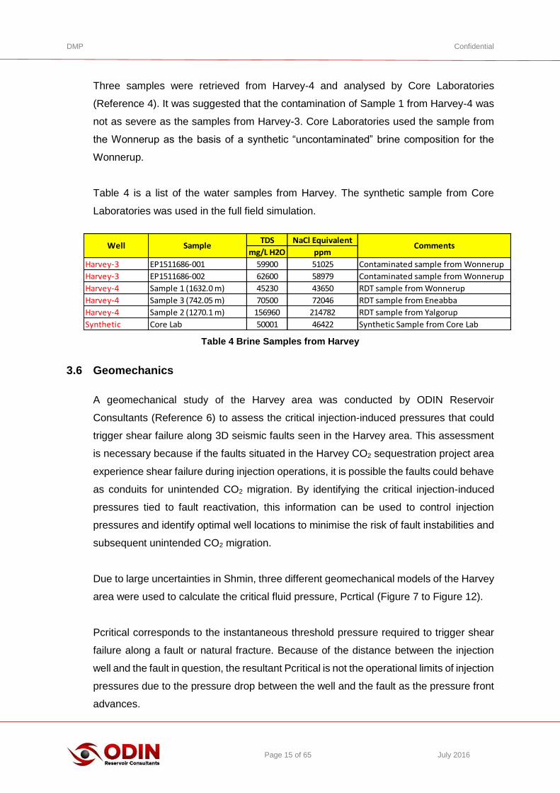
Three samples were retrieved from Harvey-4 and analysed by Core Laboratories

(Reference 4). It was suggested that the contamination of Sample 1 from Harvey-4 was

not as severe as the samples from Harvey-3. Core Laboratories used the sample from

the Wonnerup as the basis of a synthetic “uncontaminated” brine composition for the

Wonnerup.

Table 4 is a list of the water samples from Harvey. The synthetic sample from Core

Laboratories was used in the full field simulation.

Table 4 Brine Samples from Harvey

3.6 Geomechanics

A geomechanical study of the Harvey area was conducted by ODIN Reservoir

Consultants (Reference 6) to assess the critical injection-induced pressures that could

trigger shear failure along 3D seismic faults seen in the Harvey area. This assessment

is necessary because if the faults situated in the Harvey CO2 sequestration project area

experience shear failure during injection operations, it is possible the faults could behave

as conduits for unintended CO2 migration. By identifying the critical injection-induced

pressures tied to fault reactivation, this information can be used to control injection

pressures and identify optimal well locations to minimise the risk of fault instabilities and

subsequent unintended CO2 migration.

Due to large uncertainties in Shmin, three different geomechanical models of the Harvey

area were used to calculate the critical fluid pressure, Pcrtical (Figure 7 to Figure 12).

Pcritical corresponds to the instantaneous threshold pressure required to trigger shear

failure along a fault or natural fracture. Because of the distance between the injection

well and the fault in question, the resultant Pcritical is not the operational limits of injection

pressures due to the pressure drop between the well and the fault as the pressure front

advances.

TDS NaCl Equivalent

mg/L H2O ppm

Harvey-3 EP1511686-001 59900 51025 Contaminated sample from Wonnerup

Harvey-3 EP1511686-002 62600 58979 Contaminated sample from Wonnerup

Harvey-4 Sample 1 (1632.0 m) 45230 43650 RDT sample from Wonnerup

Harvey-4 Sample 3 (742.05 m) 70500 72046 RDT sample from Eneabba

Harvey-4 Sample 2 (1270.1 m) 156960 214782 RDT sample from Yalgorup

Synthetic Core Lab 50001 46422 Synthetic Sample from Core Lab

Well Sample Comments

DMP Confidential

of 65 July 2016

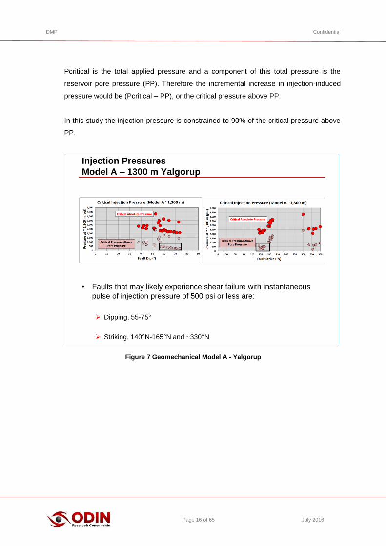
Pcritical is the total applied pressure and a component of this total pressure is the

reservoir pore pressure (PP). Therefore the incremental increase in injection-induced

pressure would be (Pcritical – PP), or the critical pressure above PP.

In this study the injection pressure is constrained to 90% of the critical pressure above

PP.

Figure 7 Geomechanical Model A - Yalgorup

Tel: +61-414-246-600

• Faults that may likely experience shear failure with instantaneous

pulse of injection pressure of 500 psi or less are:

Dipping, 55-75°

Striking, 140°N-165°N and ~330°N

Injection Pressures

Model A – 1300 m Yalgorup

DMP Confidential

of 65 July 2016

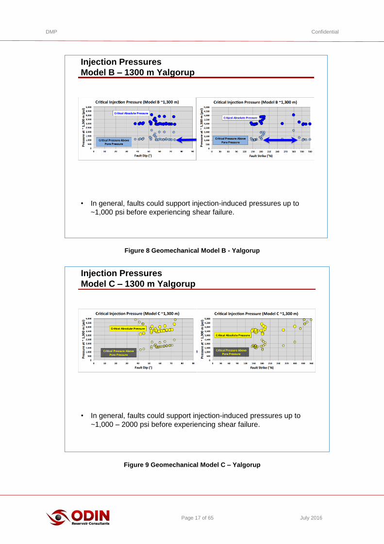
Figure 8 Geomechanical Model B - Yalgorup

Figure 9 Geomechanical Model C – Yalgorup

Tel: +61-414-246-600

• In general, faults could support injection-induced pressures up to

~1,000 psi before experiencing shear failure.

Injection Pressures

Model B – 1300 m Yalgorup

Tel: +61-414-246-600


~1,000 – 2000 psi before experiencing shear failure.

Injection Pressures

Model C – 1300 m Yalgorup

DMP Confidential

of 65 July 2016

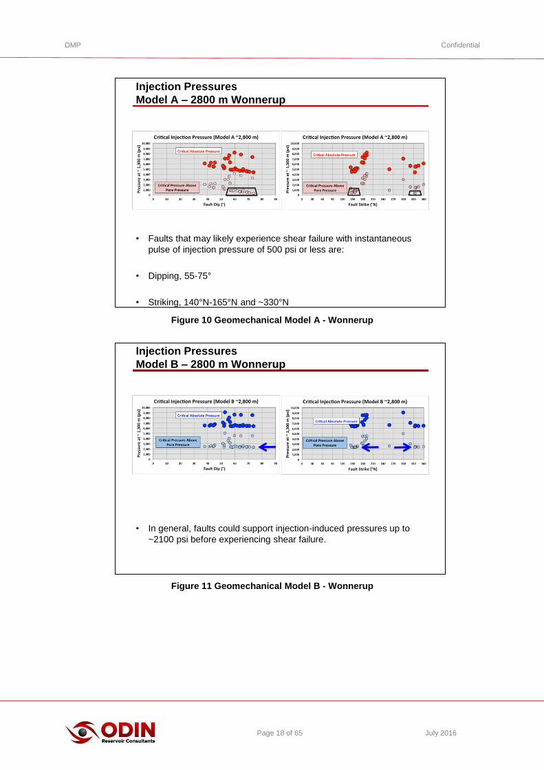
Figure 10 Geomechanical Model A - Wonnerup

Figure 11 Geomechanical Model B - Wonnerup

Page 15 Tel: +61-414-246-600

• Faults that may likely experience shear failure with instantaneous

pulse of injection pressure of 500 psi or less are:

• Dipping, 55-75°

• Striking, 140°N-165°N and ~330°N

Injection Pressures

Model A – 2800 m Wonnerup

Page 16 Tel: +61-414-246-600


~2100 psi before experiencing shear failure.

Injection Pressures

Model B – 2800 m Wonnerup

DMP Confidential

of 65 July 2016

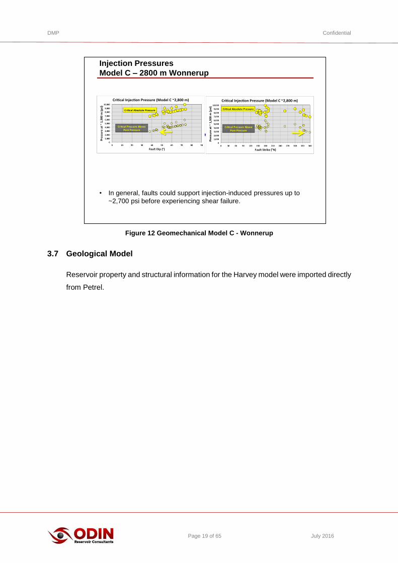
Figure 12 Geomechanical Model C - Wonnerup

3.7 Geological Model

Reservoir property and structural information for the Harvey model were imported directly

from Petrel.

Page 17 Tel: +61-414-246-600


~2,700 psi before experiencing shear failure.

Injection Pressures

Model C – 2800 m Wonnerup

DMP Confidential

of 65 July 2016

4. UPSCALING

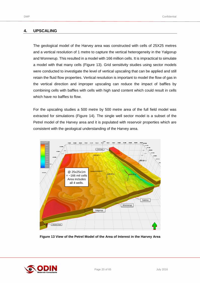
The geological model of the Harvey area was constructed with cells of 25X25 metres

and a vertical resolution of 1 metre to capture the vertical heterogeneity in the Yalgorup

and Wonnerup. This resulted in a model with 166 million cells. It is impractical to simulate

a model with that many cells (Figure 13). Grid sensitivity studies using sector models

were conducted to investigate the level of vertical upscaling that can be applied and still

retain the fluid flow properties. Vertical resolution is important to model the flow of gas in

the vertical direction and improper upscaling can reduce the impact of baffles by

combining cells with baffles with cells with high sand content which could result in cells

which have no baffles to flow.

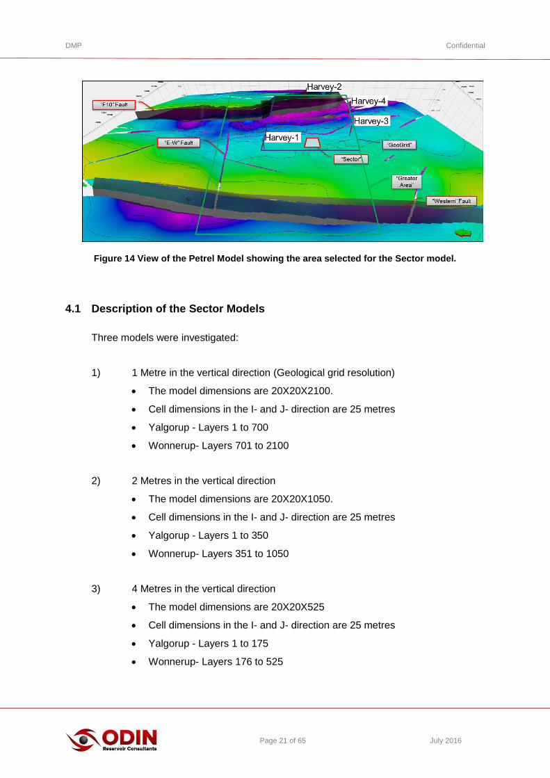
For the upscaling studies a 500 metre by 500 metre area of the full field model was

extracted for simulations (Figure 14). The single well sector model is a subset of the

Petrel model of the Harvey area and it is populated with reservoir properties which are

consistent with the geological understanding of the Harvey area.

Figure 13 View of the Petrel Model of the Area of Interest in the Harvey Area

Wonnerup

Sabina

Yalgorup

F10 Fault

Western Fault

@ 25x25x1m

= ~166 mil cells

Area includes

all 4 wells.

DMP Confidential

of 65 July 2016

Figure 14 View of the Petrel Model showing the area selected for the Sector model.

4.1 Description of the Sector Models

Three models were investigated:

1) 1 Metre in the vertical direction (Geological grid resolution)

The model dimensions are 20X20X2100.

Cell dimensions in the I- and J- direction are 25 metres

Yalgorup - Layers 1 to 700

Wonnerup- Layers 701 to 2100

2) 2 Metres in the vertical direction

The model dimensions are 20X20X1050.




3) 4 Metres in the vertical direction

The model dimensions are 20X20X525




DMP Confidential

of 65 July 2016

4.1.1 Model Run Parameters

The following parameters were used to initialise the sector model and constrain the runs.

1) Flow based upscaling in the Petrel model was used to upscale the cells in the vertical

direction.

2) For expediency, a Black Oil model was used for simulations and the Yalgorup and

Wonnerup reservoirs were run separately.

3) Dry gas PVT tables used in the simulation were generated with industry standard

correlations with gas specific gravity of 0.75.

4) Relative Permeability (Figure 17).

a. Krw @ (Sw=1) = 0.37

b. Krg @ (Swmin=0.49) = 0.12

c. Corey exponents

d. Nw= 4.0

e. Ng= 4.5

5) The model was initialised as a fully water saturated model at an initial pressure of

179 bars at a datum depth of 1801 metres.

6) A dry gas injector was located at I=10 and J=10 and dry gas was injected into the

model. Figure 15 shows the sector model.

7) The injection rate was constrained to a maximum of 457,000 m3/d (≈ 300,000 tpa).

8) The injection bottom hole pressure was constrained to Pore Pressure + 0.9*69 bars

(Geomechanics Model B).

9) Gas was injected into the models for 30 years.

10) In the Yalogorup model, the well was completed over the bottom 148 metres and in

the Wonnerup model, the well was completed over the bottom 200 metres.

DMP Confidential

of 65 July 2016

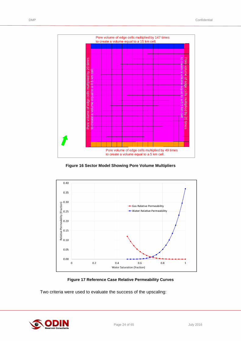
Pore volume multipliers were used to modify the edge cells of the sector model to match

the aquifer surrounding the area defined by the sector (Figure 16). Without the pore

volume multipliers the injection of the gas into the model would result in significant

increase in reservoir pressure which would lead to the injection bottom hole constraint

being violated.

Figure 15 Sector Model of the Yalgorup and Wonnerup

Page 35 Tel: +61-414-246-600

25x25x1m0.25

0.20

0.15

0.10

0.05

0.00

GRID No. Cells Min Max Average STD Min Max Average STD Min Max Average STD

25x25x1_500x500 806,011 0.000 0.318 0.119 0.062 0.0014 1958.658 247.8289 330.835 0.0014 1958.658 246.9432 331.3408

PORO PERMX PERMZ

Porosity

Top

Wonnerup

“Sector Model”

DMP Confidential

of 65 July 2016

Figure 16 Sector Model Showing Pore Volume Multipliers

Figure 17 Reference Case Relative Permeability Curves

Two criteria were used to evaluate the success of the upscaling:

Page 34 Tel: +61-414-246-600

Reference Case Parameters

Pore volume of edge cells multiplied by 147 times

to create a volume equal to a 15 km cell.

Pore volume of edge cells multiplied by 49 times

to create a volume equal to a 5 km cell.

Po

re v

olu

me

of e

dg

e c

ells m

ultip

lied b

y 2

0 tim

es

to c

rea

te a

vo

lum

e e

qu

al to

a 0

.5 k

m c

ell.

Po

re v

olu

me

of e

dg

e c

ells

mu

ltiplie

d b

y 2

0 tim

es

to c

rea

te a

vo

lum

e e

qu

al to

a 0

.5 k

m c

ell.

DMP Confidential

of 65 July 2016

The bottom hole pressure during the injection should be almost identical for the same

injection rate. This would demonstrate that the vertical connectivity is the same for the

different grids.

The saturation profiles in the models should be almost identical.

4.2 Model Results

4.2.1 Yalgorup

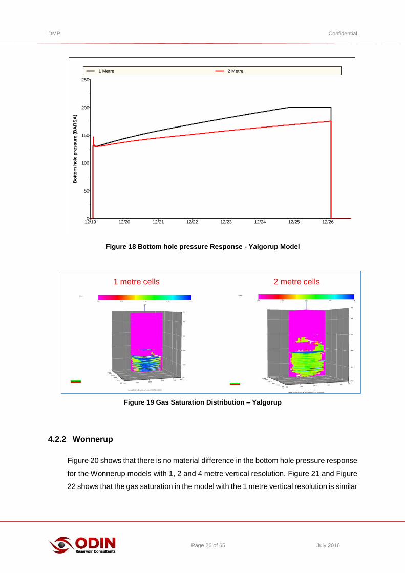
Figure 18 compares the bottom hole pressure response between the 1 metre (geological

scale) model and the model with the vertical resolution of 2 metres. The results show

that the BHP response is different in the two models. The lower injection pressures

observed in the 2 metre model indicates that it is more connected compared to the 1

metre model. This indicates that some of the vertical baffles to flow have been smoothed

out.

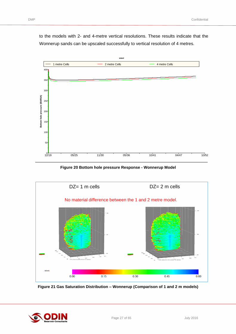
Figure 19 compares the gas saturation distribution in the model with 1 metre vertical

resolution and the model with 2 metre vertical resolution. Gas saturation distribution in

the 1 and 2 metre models at the end of run is quite different between the two models.

Gas has migrated farther up the column in the 2 metre model compared to the 1 metre

model. This indicates that the baffles to flow in the 1 metre model were “smoothed” out.

The results of the upscaling runs with the Yalgorup model indicates that vertical upscaling

is not suitable for this sand.

DMP Confidential

of 65 July 2016

Figure 18 Bottom hole pressure Response - Yalgorup Model

Figure 19 Gas Saturation Distribution – Yalgorup

4.2.2 Wonnerup

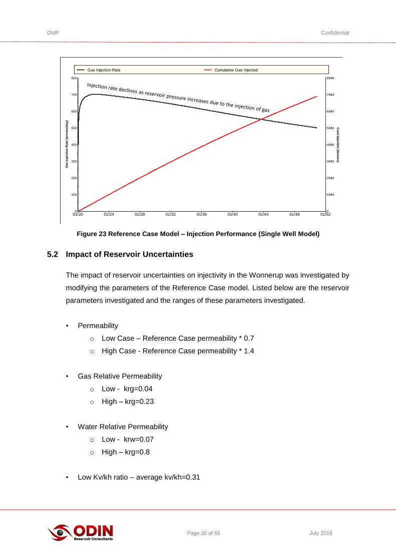
Figure 20 shows that there is no material difference in the bottom hole pressure response

for the Wonnerup models with 1, 2 and 4 metre vertical resolution. Figure 21 and Figure

22 shows that the gas saturation in the model with the 1 metre vertical resolution is similar

12/19 12/20 12/21 12/22 12/23 12/24 12/25 12/260

50

100

150

200

250B

ott

om

ho

le p

ressu

re (

BA

RS

A)

1 Metre 2 Metre

Page 26 Tel: +61-414-246-600

Model Results @ end of simulation

Gas Saturation Distribution - Yalgorup

1 metre cells 2 metre cells

DMP Confidential

of 65 July 2016

to the models with 2- and 4-metre vertical resolutions. These results indicate that the

Wonnerup sands can be upscaled successfully to vertical resolution of 4 metres.

Figure 20 Bottom hole pressure Response - Wonnerup Model

Figure 21 Gas Saturation Distribution – Wonnerup (Comparison of 1 and 2 m models)

12/19 05/25 11/30 05/36 10/41 04/47 10/520

50

100

150

200

250

300

350

400

Bo

tto

m h

ole

pre

ss

ure

(B

AR

SA

)

WBHP

1 metre Cells 2 metre Cells 4 metre Cells

Page 28 Tel: +61-414-246-600

Upscaling Study – Wonnerup Sands

Comparison of Gas Saturation Distribution

DZ= 1 m cells DZ= 2 m cells

No material difference between the 1 and 2 metre model.

DMP Confidential

of 65 July 2016

Figure 22 Gas Saturation Distribution – Wonnerup (Comparison of 1 and 4 m models)

Page 29 Tel: +61-414-246-600

Upscaling Study – Wonnerup Sands

Comparison of Gas Saturation Distribution

DZ= 1 metre cells DZ= 4 metre cells

Minor differences in gas distribution between the 1 and 4 metre model.

The results of the grid sensitivity modelling shows that the Wonnerup model

can be successfully upscaled to a vertical resolution of 4 metres.

DMP Confidential

of 65 July 2016

5. INJECTIVITY STUDIES

This phase of the dynamic modelling was conducted using the Wonnerup model with a

vertical resolution of 4 metres. The objective of the study is to obtain probabilistic

distribution of injection rates in the Wonnerup at a notional injection capacity of 3 -10

million tonnes per annum per well. As a guide ODIN is using a conceptual scenario of a

project with 9-10 wells.

5.1 Reference Case

The Reference Case is defined below:

• Bottom hole pressure constraint = 360 bars @ 2948 m [Pore Pressure + 0.9*69 bar]i

• Average kv/kh = 0.75 derived from Petrel model

• No damage skin.

• Well is completed in the bottom 250 metres for kh=20330 mD-m.

• Arbitrary start date of 1/1/2020

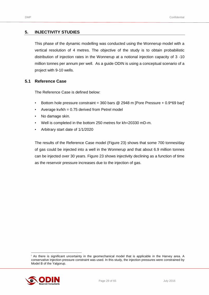
The results of the Reference Case model (Figure 23) shows that some 700 tonnes/day

of gas could be injected into a well in the Wonnerup and that about 6.9 million tonnes

can be injected over 30 years. Figure 23 shows injectivity declining as a function of time

as the reservoir pressure increases due to the injection of gas.

i As there is significant uncertainty in the geomechanical model that is applicable in the Harvey area. A conservative injection pressure constraint was used. In this study, the injection pressures were constrained by Model B of the Yalgorup.

DMP Confidential

of 65 July 2016

Figure 23 Reference Case Model – Injection Performance (Single Well Model)

5.2 Impact of Reservoir Uncertainties

The impact of reservoir uncertainties on injectivity in the Wonnerup was investigated by

modifying the parameters of the Reference Case model. Listed below are the reservoir

parameters investigated and the ranges of these parameters investigated.

• Permeability

o Low Case – Reference Case permeability * 0.7

o High Case - Reference Case permeability * 1.4

• Gas Relative Permeability

o Low - krg=0.04

o High – krg=0.23

• Water Relative Permeability

o Low - krw=0.07

o High – krg=0.8

• Low Kv/kh ratio – average kv/kh=0.31

01/20 01/24 01/28 01/32 01/36 01/40 01/44 01/48 01/520

100

200

300

400

500

600

700

800

Ga

s In

jec

tio

n R

ate

(to

nn

es

/da

y)

0

1MM

2MM

3MM

4MM

5MM

6MM

7MM

8MM

Cu

m In

jec

tion

(ton

ne

s)

Gas Injection Rate Cumulative Gas Injected

DMP Confidential

of 65 July 2016

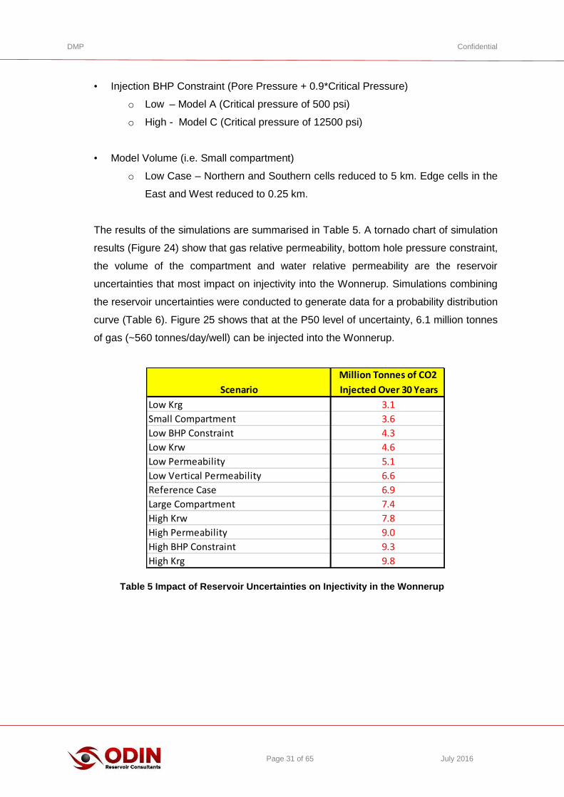
• Injection BHP Constraint (Pore Pressure + 0.9*Critical Pressure)

o Low – Model A (Critical pressure of 500 psi)

o High - Model C (Critical pressure of 12500 psi)

• Model Volume (i.e. Small compartment)

o Low Case – Northern and Southern cells reduced to 5 km. Edge cells in the

East and West reduced to 0.25 km.

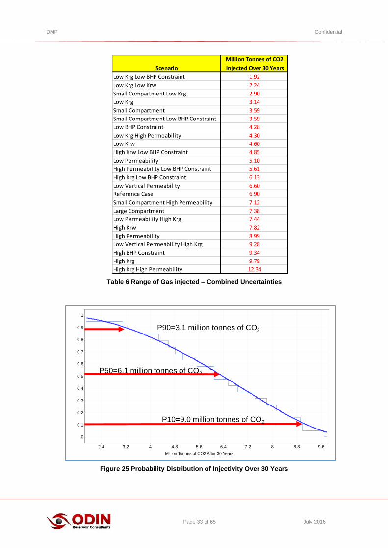
The results of the simulations are summarised in Table 5. A tornado chart of simulation

results (Figure 24) show that gas relative permeability, bottom hole pressure constraint,

the volume of the compartment and water relative permeability are the reservoir

uncertainties that most impact on injectivity into the Wonnerup. Simulations combining

the reservoir uncertainties were conducted to generate data for a probability distribution

curve (Table 6). Figure 25 shows that at the P50 level of uncertainty, 6.1 million tonnes

of gas (~560 tonnes/day/well) can be injected into the Wonnerup.

Table 5 Impact of Reservoir Uncertainties on Injectivity in the Wonnerup

Scenario

Million Tonnes of CO2

Injected Over 30 Years

Low Krg 3.1

Small Compartment 3.6

Low BHP Constraint 4.3

Low Krw 4.6

Low Permeability 5.1

Low Vertical Permeability 6.6

Reference Case 6.9

Large Compartment 7.4

High Krw 7.8

High Permeability 9.0

High BHP Constraint 9.3

High Krg 9.8

DMP Confidential

of 65 July 2016

Figure 24 Tornado Chart Showing Impact of Reservoir Uncertainties on Injectivity

Tel: +61-414-246-600

Tornado Chart of Reservoir Uncertainties

Reference Case = 6.9 million Tonnes

85% of the

total

Uncertainty

DMP Confidential

of 65 July 2016

Table 6 Range of Gas injected – Combined Uncertainties

Figure 25 Probability Distribution of Injectivity Over 30 Years

Scenario

Million Tonnes of CO2

Injected Over 30 Years

Low Krg Low BHP Constraint 1.92

Low Krg Low Krw 2.24

Small Compartment Low Krg 2.90

Low Krg 3.14

Small Compartment 3.59

Small Compartment Low BHP Constraint 3.59

Low BHP Constraint 4.28

Low Krg High Permeability 4.30

Low Krw 4.60

High Krw Low BHP Constraint 4.85

Low Permeability 5.10

High Permeability Low BHP Constraint 5.61

High Krg Low BHP Constraint 6.13

Low Vertical Permeability 6.60

Reference Case 6.90

Small Compartment High Permeability 7.12

Large Compartment 7.38

Low Permeability High Krg 7.44

High Krw 7.82

High Permeability 8.99

Low Vertical Permeability High Krg 9.28

High BHP Constraint 9.34

High Krg 9.78

High Krg High Permeability 12.34

Page 37 Tel: +61-414-246-600

Tonnes of CO2 After 30 Years

9.68.887.26.45.64.843.22.4

Cum

ula

tive P

robabili

ty

1

0.9

0.8

0.7

0.6

0.5

0.4

0.3

0.2

0.1

0

Probability Distribution of Injectivity after 30 Years

Single Well Model

P50=6.1 million tonnes of CO2



Million Tonnes of CO2 After 30 Years

DMP Confidential

of 65 July 2016

6. MODELLING OF THE CO2 PLUME

This phase of the study is focussed on the full field modelling of the movement of the

CO2 plume after 30 years of injection at 800,000 tonnes per annum and 1000 years of

shut-in. The full field model integrates all of the available subsurface information into a

dynamic reservoir model that represents and describes the fluid flow processes in the

reservoir.

To enable the simulations to be conducted in a reasonable time, a coarse scale model

of the Harvey area was constructed to investigate plume movement in the Harvey area

during and after injection of the planned CO2 volume.

6.1 Simulator Selection

The full field model of the Harvey area was constructed in the compositional simulator,

GEMS™ (Version 2015.10). GEMSii is a full featured compositional simulator and

capable of modelling:

• Hysteresis and residual gas trapping.

• Gas solubility in aqueous phase.

• Vaporization of water during CO2 injection.

• Detailed calculations of brine density, viscosity and accounts for solubility of CO2 in

the brine.

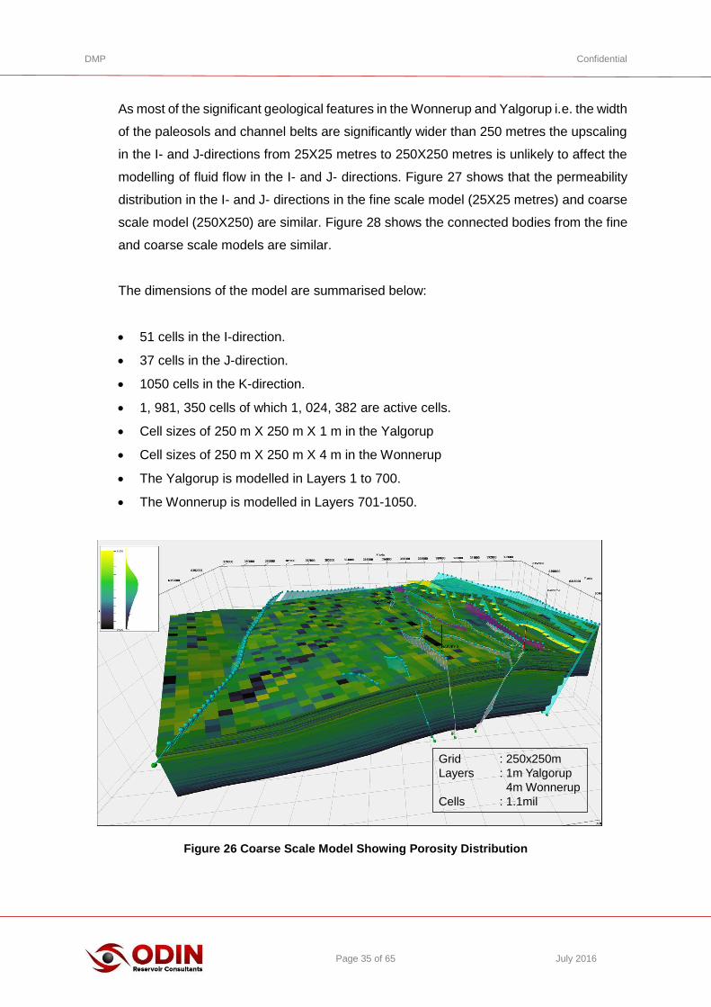
6.2 Model Description

The model was constructed with grid blocks of 250X250 metres in the I- and J-directions

with the resolution of the layers in the Yalgorup retained at the geological model scale of

1 metre. In the Wonnerup, the 4 metre layers were used (Figure 26). To further reduce

the number of cells in the full field model, all cells with a depth shallower than 800

mTVDss was made void. Migration of CO2 shallower than 800 mTVDss is considered a

breach of containment as the CO2 changes from a supercritical state to a gaseous state

at depths shallower than 800 mTVDss.

ii GEMS is a trademark of Computer Modelling Group (CMG)

DMP Confidential

of 65 July 2016

As most of the significant geological features in the Wonnerup and Yalgorup i.e. the width

of the paleosols and channel belts are significantly wider than 250 metres the upscaling

in the I- and J-directions from 25X25 metres to 250X250 metres is unlikely to affect the

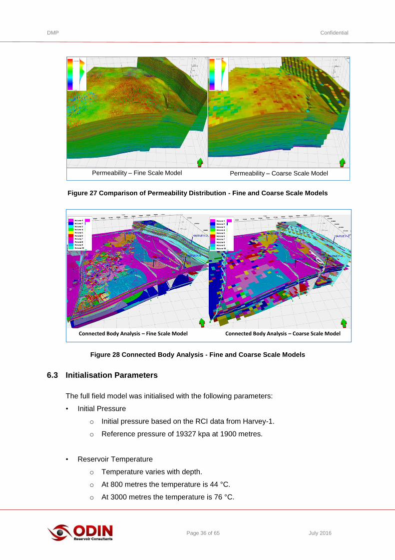
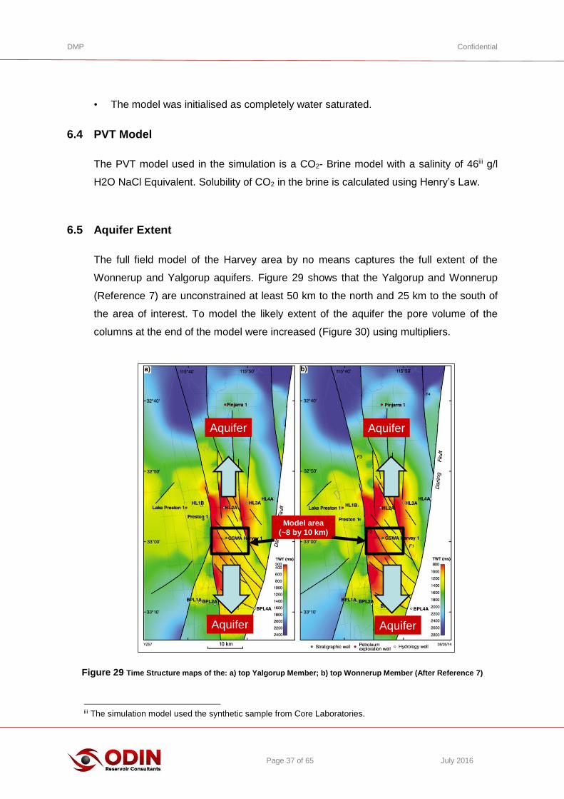
modelling of fluid flow in the I- and J- directions. Figure 27 shows that the permeability

distribution in the I- and J- directions in the fine scale model (25X25 metres) and coarse

scale model (250X250) are similar. Figure 28 shows the connected bodies from the fine

and coarse scale models are similar.

The dimensions of the model are summarised below:

51 cells in the I-direction.

37 cells in the J-direction.

1050 cells in the K-direction.

1, 981, 350 cells of which 1, 024, 382 are active cells.

Cell sizes of 250 m X 250 m X 1 m in the Yalgorup

Cell sizes of 250 m X 250 m X 4 m in the Wonnerup

The Yalgorup is modelled in Layers 1 to 700.

The Wonnerup is modelled in Layers 701-1050.

Figure 26 Coarse Scale Model Showing Porosity Distribution

Grid : 250x250m

Layers : 1m Yalgorup

4m Wonnerup

Cells : 1.1mil

DMP Confidential

of 65 July 2016

Figure 27 Comparison of Permeability Distribution - Fine and Coarse Scale Models

Figure 28 Connected Body Analysis - Fine and Coarse Scale Models

6.3 Initialisation Parameters

The full field model was initialised with the following parameters:

• Initial Pressure

o Initial pressure based on the RCI data from Harvey-1.

o Reference pressure of 19327 kpa at 1900 metres.

• Reservoir Temperature

o Temperature varies with depth.

o At 800 metres the temperature is 44 °C.

o At 3000 metres the temperature is 76 °C.

Page 40 Tel: +61-414-246-600

Top

Sabina

Top

Wonnerup

Top

Yalgorup

H-2

H-4H-3

H-1H-2

H-4H-3

H-1

Top

Sabina

Top

Wonnerup

Top

Yalgorup

Permeability – Fine Scale Model Permeability – Coarse Scale Model

Connected Body Analysis – Fine Scale Model Connected Body Analysis – Coarse Scale Model

DMP Confidential

of 65 July 2016

• The model was initialised as completely water saturated.

6.4 PVT Model

The PVT model used in the simulation is a CO2- Brine model with a salinity of 46iii g/l

H2O NaCl Equivalent. Solubility of CO2 in the brine is calculated using Henry’s Law.

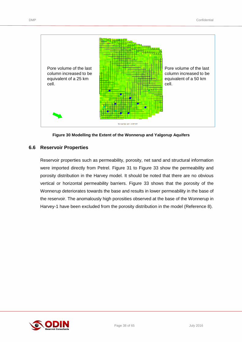
6.5 Aquifer Extent

The full field model of the Harvey area by no means captures the full extent of the

Wonnerup and Yalgorup aquifers. Figure 29 shows that the Yalgorup and Wonnerup

(Reference 7) are unconstrained at least 50 km to the north and 25 km to the south of

the area of interest. To model the likely extent of the aquifer the pore volume of the

columns at the end of the model were increased (Figure 30) using multipliers.

Figure 29 Time Structure maps of the: a) top Yalgorup Member; b) top Wonnerup Member (After Reference 7)

iii The simulation model used the synthetic sample from Core Laboratories.

Page 10 Tel: +61-414-246-600

Model area

(~8 by 10 km)

Aquifer

AquiferAquifer

Aquifer

DMP Confidential

of 65 July 2016

Figure 30 Modelling the Extent of the Wonnerup and Yalgorup Aquifers

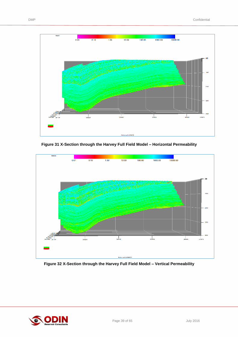
6.6 Reservoir Properties

Reservoir properties such as permeability, porosity, net sand and structural information

were imported directly from Petrel. Figure 31 to Figure 33 show the permeability and

porosity distribution in the Harvey model. It should be noted that there are no obvious

vertical or horizontal permeability barriers. Figure 33 shows that the porosity of the

Wonnerup deteriorates towards the base and results in lower permeability in the base of

the reservoir. The anomalously high porosities observed at the base of the Wonnerup in

Harvey-1 have been excluded from the porosity distribution in the model (Reference 8).

Page 11 Tel: +61-414-246-600

Aquifer Extent

Pore volume of the last

column increased to be

equivalent of a 25 km

cell.

Pore volume of the last

column increased to be

equivalent of a 50 km

cell.

DMP Confidential

of 65 July 2016

Figure 31 X-Section through the Harvey Full Field Model – Horizontal Permeability

Figure 32 X-Section through the Harvey Full Field Model – Vertical Permeability

DMP Confidential

of 65 July 2016

Figure 33 X-Section through the Harvey Full Field Model – Porosity

6.7 Conceptual Development Plan – Reference Case

The conceptual development plan for the Harvey area envisages injection of 800,000

tonnes of CO2 per year for 30 years. At the end of the 30 year injection period, the wells

are shut-in and the CO2 is allowed to dissipate through the aquifer. In this work, it was

assumed that 9 wells laid out in a staggered line-drive configuration would be used to

inject CO2 into the Wonnerup reservoir. All of the wells are completed in the bottom 250

metres of the Wonnerup.

6.7.1 Reference Case Definition

The Reference Case for the conceptual development study is defined as follows:

• Reservoir

o All faults are assumed to be not sealing.

o Wonnerup and Yalgorup are assumed to be in communication.

• PVT Properties

• NaCl concentration of 46 g/L H2O.

DMP Confidential

of 65 July 2016

o No mineralisation is assumed.

o Model includes the solubility of CO2 in brine.

o Injection fluid assumed to be 100% CO2.

• Rock-Fluid

o Hysteresis of the gas phase is assumed.

o Trapped gas saturation, SgT = 0.19

o No hysteresis of the water phase

• Injection

o CO2 is injected at rate of 800,000 tonnes per annum through 9 wells.

o Injection begins on an arbitrary date of 1/1/2020 and ends on 10/1/2050.

o Bottom hole pressure constraint = 360 bars @ 2948 m [Pore Pressure +

0.9*69 bars]

• In the simulation model, relative permeability curves were generated using the

following Corey exponents and end points:

o Nw= 4.0

o Ng= 4.5

o Krw @ (Sw=1) = 0.37

o Krg @ (Swmin=0.49) = 0.12

6.7.2 Results

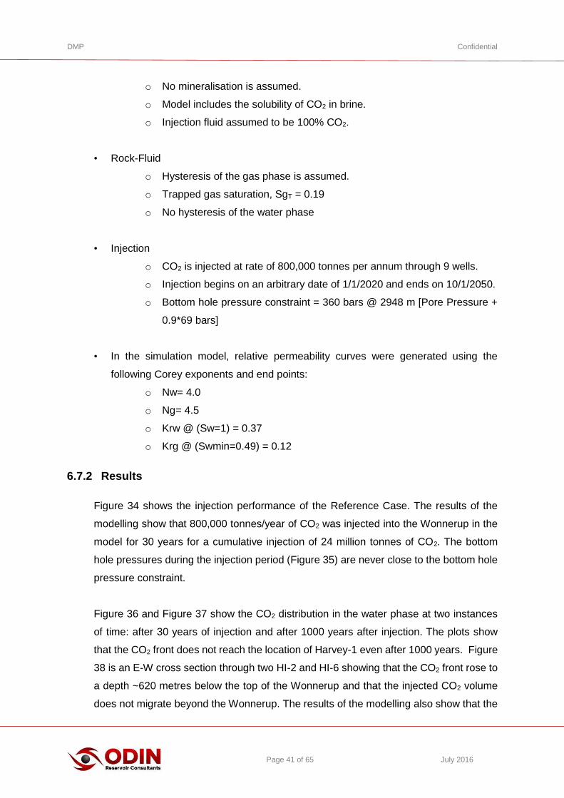
Figure 34 shows the injection performance of the Reference Case. The results of the

modelling show that 800,000 tonnes/year of CO2 was injected into the Wonnerup in the

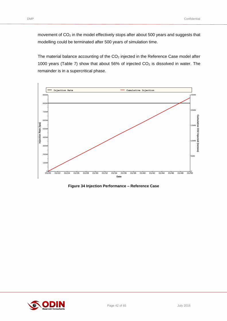
model for 30 years for a cumulative injection of 24 million tonnes of CO2. The bottom

hole pressures during the injection period (Figure 35) are never close to the bottom hole

pressure constraint.

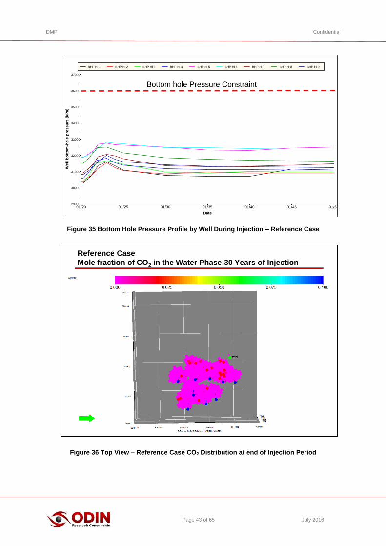
Figure 36 and Figure 37 show the CO2 distribution in the water phase at two instances

of time: after 30 years of injection and after 1000 years after injection. The plots show

that the CO2 front does not reach the location of Harvey-1 even after 1000 years. Figure

38 is an E-W cross section through two HI-2 and HI-6 showing that the CO2 front rose to

a depth ~620 metres below the top of the Wonnerup and that the injected CO2 volume

does not migrate beyond the Wonnerup. The results of the modelling also show that the

DMP Confidential

of 65 July 2016

movement of CO2 in the model effectively stops after about 500 years and suggests that

modelling could be terminated after 500 years of simulation time.

The material balance accounting of the CO2 injected in the Reference Case model after

1000 years (Table 7) show that about 56% of injected CO2 is dissolved in water. The

remainder is in a supercritical phase.

Figure 34 Injection Performance – Reference Case

01/20 01/22 01/24 01/26 01/28 01/30 01/32 01/34 01/36 01/38 01/40 01/42 01/44 01/46 01/48 01/50

Date

0

100M

200M

300M

400M

500M

600M

700M

800M

900M

Inje

cti

on

Ra

te (

tpa

)

0

5MM

10MM

15MM

20MM

25MM

Cu

mu

lativ

e C

O2 In

jecte

d (to

nn

es)

Injection Rate Cumulative Injection

DMP Confidential

of 65 July 2016

Figure 35 Bottom Hole Pressure Profile by Well During Injection – Reference Case

Figure 36 Top View – Reference Case CO2 Distribution at end of Injection Period

01/20 01/25 01/30 01/35 01/40 01/45 01/50

Date

29000

30000

31000

32000

33000

34000

35000

36000

37000

Well

bo

tto

m-h

ole

pre

ssu

re (

kP

a)

BHP HI-1 BHP HI-2 BHP HI-3 BHP HI-4 BHP HI-5 BHP HI-6 BHP HI-7 BHP HI-8 BHP HI-9

Bottom hole Pressure Constraint

Page 59 Tel: +61-414-246-600

Reference Case

Mole fraction of CO2 in the Water Phase 30 Years of Injection

DMP Confidential

of 65 July 2016

Figure 37 Top View – Reference Case CO2 Distribution 1000 years after injection

Figure 38 Reference Case – X-Section through HI-2 and HI-6

Page 60 Tel: +61-414-246-600

Mole fraction of CO2 in the Water Phase 1000 Years After the Cessation of Injection

Plume is ~7X7 km

Page 61 Tel: +61-414-246-600

Mole fraction of CO2 in the Water Phase 1000 Years After the Cessation of Injection

Cross Section Through HI-2 and JI-6

Plume is ~7X7 km

DMP Confidential

of 65 July 2016

Table 7 Material Balance Accounting (1000 Years after Injection)

6.8 Impact of Reservoir Uncertainties on the movement of the CO2 plume

A number of models of the Harvey area were constructed to investigate the effects of the

reservoir uncertainties on containment failure and the location of the CO2 plume in

relation to the abandoned Harvey-1 well. Table 8 is a summary of the reservoir

uncertainties investigated and the parameters used in the investigations.

Table 8 Case Summary – Full Field Model of the Harvey Area

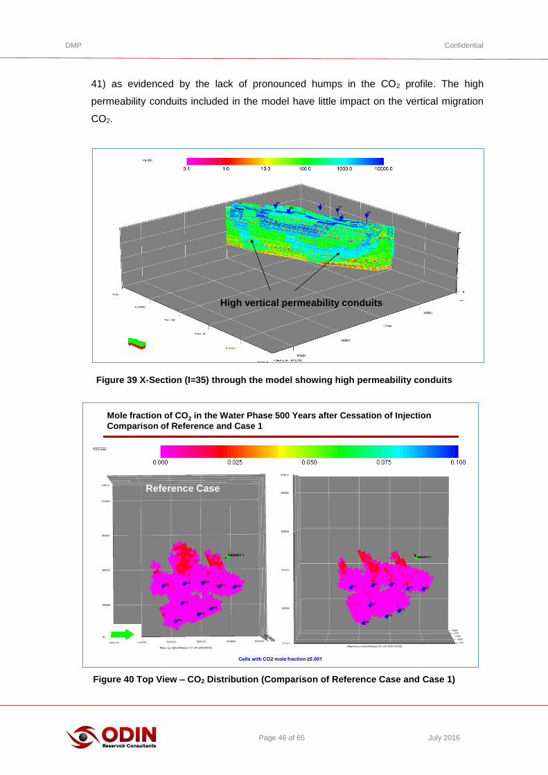
6.8.1 Case 1 – High Vertical Permeability (“Holey Faults”)

The area of interest in the Harvey area is intersected by a number of faults. None of

these faults are expected to form lateral barriers to flow but the areas near the faults may

have enhanced vertical permeability due to fractures. In Case 1, these fracture zones

are modelled as areas of enhanced vertical permeability. The vertical permeability of

cells adjacent to a fault are increased 10 times.

Figure 40 compares the distribution of CO2 in the Reference Case and Case 1 after 500

years. The distribution of CO2 in Case 1 is more compact compared to the Reference

Case as a result of the CO2 being more evenly distributed in the shallower layers (Figure

CO2 Storage Amounts in the Reservoir Moles % of Moles InjectedGaseous Phase 0 0%

Liquid Phase 0 0%

Dissolved in Water 3.13E+11 55%

Total Supercritical Phase 2.58E+11 45%

Supercritical Phase Trapped (Sgc or Hysteresis) 2.52E+11 44%

Supercritical Phase not trapped 6.00E+09 1%

Case Model NameGeological

Model

Trapped Gas

Saturation

Brine Salinity

(g/L NaCl Eq.)

Internal

Faults

End Point Gas

Relative PermeabilityReference Reference Reference 0.19 45600 Not sealing 0.12

1 Holey Faults

Vertical permeability of cells

adjacent to faults is increased by

10 times.

0.19 45600 Not sealing 0.12

2 HighKrg Reference 0.19 45600 Not sealing 0.23

3 LoHyst Reference 0.10 45600 Not sealing 0.12

4 HighPermProportion of High Energy Facies

in Wonnerup Increased to 90%.0.19 45600 Not sealing 0.12

5 HikvkhVertical and horizontal

permeability are equal.0.19 45600 Not sealing 0.12

6 Seismic_Trend

Used Seismic Trend

(Deterministic Case) to populate

Paleosols in the Wonnerup.

0.19 45600 Not sealing 0.12

7 Fault_Trans Reference 0.19 45600Fault transmissibility

multiplier of 0.10.12

8 LoSol Reference 0.19 200000 Not sealing 0.12

DMP Confidential

of 65 July 2016

41) as evidenced by the lack of pronounced humps in the CO2 profile. The high

permeability conduits included in the model have little impact on the vertical migration

CO2.

Figure 39 X-Section (I=35) through the model showing high permeability conduits

Figure 40 Top View – CO2 Distribution (Comparison of Reference Case and Case 1)

Page 68 Tel: +61-414-246-600

X-Section Through Reservoir Showing High Permeability Conduits

High vertical permeability conduits

Page 69 Tel: +61-414-246-600

Mole fraction of CO2 in the Water Phase 500 Years after Cessation of Injection

Comparison of Reference and Case 1

Reference Case Case 1

Cells with CO2 mole fraction ≥0.001

DMP Confidential

of 65 July 2016

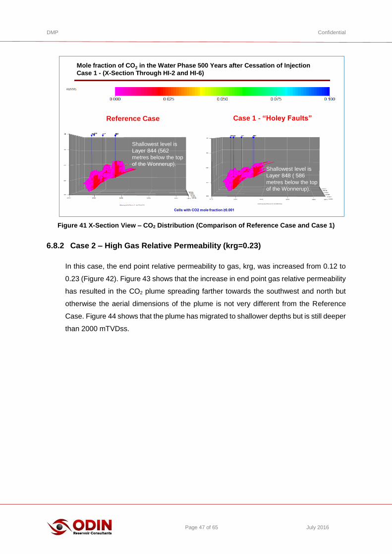
Figure 41 X-Section View – CO2 Distribution (Comparison of Reference Case and Case 1)

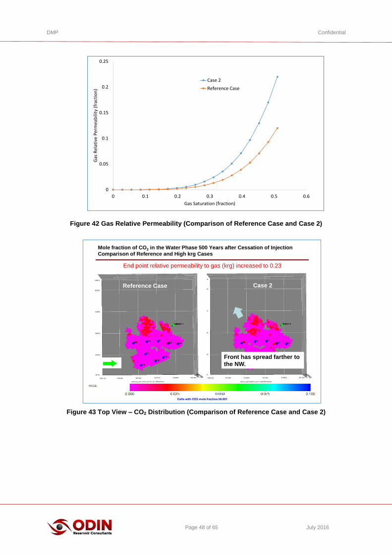
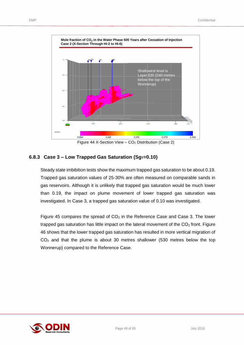
6.8.2 Case 2 – High Gas Relative Permeability (krg=0.23)

In this case, the end point relative permeability to gas, krg, was increased from 0.12 to

0.23 (Figure 42). Figure 43 shows that the increase in end point gas relative permeability

has resulted in the CO2 plume spreading farther towards the southwest and north but

otherwise the aerial dimensions of the plume is not very different from the Reference

Case. Figure 44 shows that the plume has migrated to shallower depths but is still deeper

than 2000 mTVDss.

Page 70 Tel: +61-414-246-600


Case 1 - (X-Section Through HI-2 and HI-6)

Reference Case Case 1 - “Holey Faults”

Shallowest level is

Layer 844 (562

metres below the top

of the Wonnerup).Shallowest level is

Layer 848 ( 586

metres below the top

of the Wonnerup).


DMP Confidential

of 65 July 2016

Figure 42 Gas Relative Permeability (Comparison of Reference Case and Case 2)


0

0.05

0.1

0.15

0.2

0.25

0 0.1 0.2 0.3 0.4 0.5 0.6

Gas

Rel

ativ

e Pe

rmea

bili

ty (

frac

tio

n)

Gas Saturation (fraction)

Case 2

Reference Case

Page 73 Tel: +61-414-246-600


Comparison of Reference and High krg Cases


Front has spread farther to

the NW.

End point relative permeability to gas (krg) increased to 0.23


DMP Confidential

of 65 July 2016

Figure 44 X-Section View – CO2 Distribution (Case 2)

6.8.3 Case 3 – Low Trapped Gas Saturation (SgT=0.10)

Steady state imbibition tests show the maximum trapped gas saturation to be about 0.19.

Trapped gas saturation values of 25-30% are often measured on comparable sands in

gas reservoirs. Although it is unlikely that trapped gas saturation would be much lower

than 0.19, the impact on plume movement of lower trapped gas saturation was

investigated. In Case 3, a trapped gas saturation value of 0.10 was investigated.

Figure 45 compares the spread of CO2 in the Reference Case and Case 3. The lower

trapped gas saturation has little impact on the lateral movement of the CO2 front. Figure

46 shows that the lower trapped gas saturation has resulted in more vertical migration of

CO2 and that the plume is about 30 metres shallower (530 metres below the top

Wonnerup) compared to the Reference Case.

Page 74 Tel: +61-414-246-600


Case 2 (X-Section Through HI-2 to HI-6)

Shallowest level is

Layer 835 (540 metres

below the top of the

Wonnerup)


DMP Confidential

of 65 July 2016



6.8.4 Case 4 - High Permeability Case

In this scenario, the proportion of high energy facies in the Wonnerup was increased to

90%. This has resulted in an increase in the average permeability to 357 mD compared

to 199 mD in the Reference Case. Figure 47 shows that the CO2 plume has not spread

Page 77 Tel: +61-414-246-600


Comparison of Reference and Low Trapped Gas Cases



Page 78 Tel: +61-414-246-600


Low Trapped Gas Case (X-Section Through HI-2 to HI-6)

Shallowest level is

Layer 832 (528 metres

below the top of the

Wonnerup).


DMP Confidential

of 65 July 2016

as much to the SW but towards the North and Northwest. This spread towards the North

and Northwest means that the plume has not migrated as much vertically.



Page 80 Tel: +61-414-246-600


Comparison of Reference and High Permeability Cases

Reference Case

Case 4

The front is more compact

compared to the Reference Case

and spreads more sideways.


Page 81 Tel: +61-414-246-600



Shallowest level is Layer

905 (820 metres below the

top of the Wonnerup)


DMP Confidential

of 65 July 2016

6.8.5 Case 5 – High kv/kh (Vertical to Horizontal Permeability Ratio)

In this scenario the vertical permeability in the cells are made equal to the horizontal

permeability in the fine scale Petrel model and the upscaled permeability is imported into

the simulation model. This increased the kv/kh from 0.91 in the Reference Case to 1.0 in

Case 5. Figure 49 shows that the increase in kv/kh has little impact on the aerial extent

of the CO2 plume. The increase in kv/kh did promote the migration of CO2 vertically

(Figure 50) but the effect was modest.


Page 80 Tel: +61-414-246-600


Comparison of Reference and High kv/kh Cases


Little difference in the spread

of the CO2 front compared to

the Reference Case


DMP Confidential

of 65 July 2016


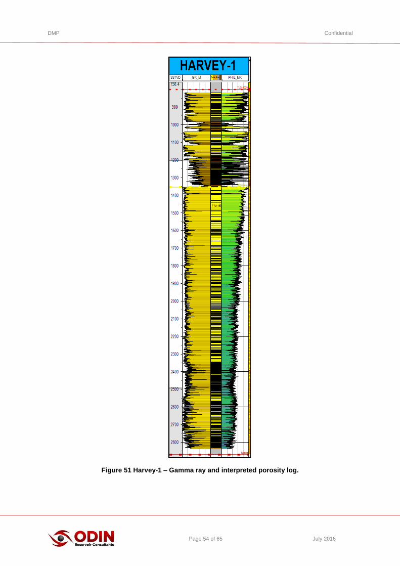
6.8.6 Case 6 – Deterministic Scenario

In this scenario, the seismic trend is used to populate the paleosols in the Petrel model.

Harvey-1 is the only well that has penetrated the full thickness of the Wonnerup sands.

The data from the well shows the Wonnerup to have a high proportion of sand and

relative homogeneous (Figure 51). This is consistent with the seismic data which is

relatively bland in the area in which Harvey-1 is located. Towards Harvey-4, the seismic

data becomes noisier and suggests a possible change in the character of the reservoir.

To model this change in character the Wonnerup in the Petrel model was

deterministically populated with paleosols.

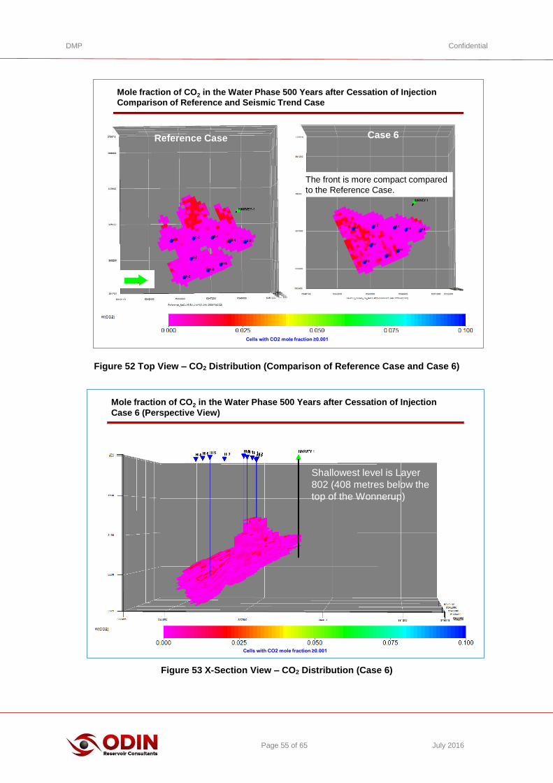
Figure 52 shows that the shape of the CO2 plume has changed significantly and is more

compact because of the distribution of the paleosols. The compactness of the CO2 plume

means that more of the CO2 migrates vertically (Figure 53).

Page 81 Tel: +61-414-246-600







DMP Confidential

of 65 July 2016

Figure 51 Harvey-1 – Gamma ray and interpreted porosity log.

DMP Confidential

of 65 July 2016



Page 83 Tel: +61-414-246-600


Comparison of Reference and Seismic Trend Case


The front is more compact compared

to the Reference Case.


Page 84 Tel: +61-414-246-600


Case 6 (Perspective View)





DMP Confidential

of 65 July 2016

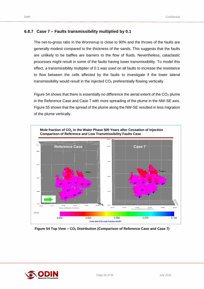
6.8.7 Case 7 – Faults transmissibility multiplied by 0.1

The net-to-gross ratio in the Wonnerup is close to 90% and the throws of the faults are

generally modest compared to the thickness of the sands. This suggests that the faults

are unlikely to be baffles are barriers to the flow of fluids. Nevertheless, cataclastic

processes might result in some of the faults having lower transmissibility. To model this

effect, a transmissibility multiplier of 0.1 was used on all faults to increase the resistance

to flow between the cells affected by the faults to investigate if the lower lateral

transmissibility would result in the injected CO2 preferentially flowing vertically.

Figure 54 shows that there is essentially no difference the aerial extent of the CO2 plume

in the Reference Case and Case 7 with more spreading of the plume in the NW-SE axis.

Figure 55 shows that the spread of the plume along the NW-SE resulted in less migration

of the plume vertically.


Page 87 Tel: +61-414-246-600


Comparison of Reference and Low Transmissibility Faults Case



DMP Confidential

of 65 July 2016


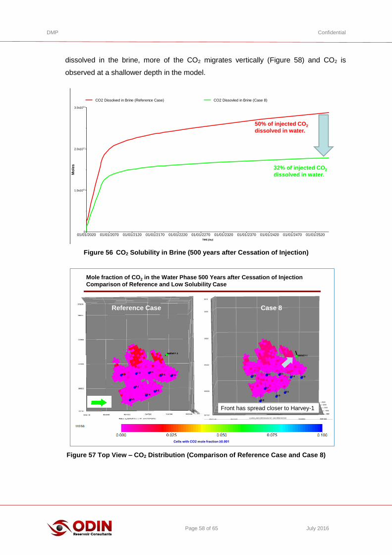
6.8.8 Case 8 – Low CO2 Solubility

The use of large grid used in the simulation of CO2 injection processes can lead to

uncertainty in the amount of CO2 dissolved in the formation brine. During the injection

stage of the storage project, the large grid blocks used in simulations resulted in an

overestimate of the amount of CO2 dissolved in the brine (Reference 9). To address the

issue raised by Reference 9, we investigated the impact on the plume movement by

reducing the solubility of CO2 in brine by assuming a brine salinity of 200 g/L H2O NaCl

Equivalent.

Figure 56 compares the number of moles of CO2 dissolved in the brine in Case 8 and

the Reference Case. The increase in the brine salinity resulted in an almost 20%

reduction of CO2 dissolved in the brine and an increase in the number of moles in the

supercritical phase.

Figure 57 shows that decreasing the solubility of CO2 in the brine has resulted in a small

change in the areal extent of the plume particularly towards the NW. With less gas

Page 88 Tel: +61-414-246-600


Case 7 (Perspective View)





DMP Confidential

of 65 July 2016

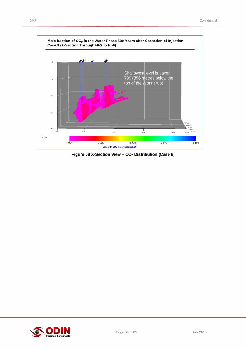
dissolved in the brine, more of the CO2 migrates vertically (Figure 58) and CO2 is

observed at a shallower depth in the model.

Figure 56 CO2 Solubility in Brine (500 years after Cessation of Injection)


01/01/2020 01/01/2070 01/01/2120 01/01/2170 01/01/2220 01/01/2270 01/01/2320 01/01/2370 01/01/2420 01/01/2470 01/01/2520

TIME (day)

0

111.0x10

112.0x10

113.0x10

Mo

les

CO2 Dissolved in Brine (Reference Case) CO2 Dissovled in Brine (Case 8)

32% of injected CO2

dissolved in water.

50% of injected CO2

dissolved in water.

Page 91 Tel: +61-414-246-600


Comparison of Reference and Low Solubility Case


Front has spread closer to Harvey-1


DMP Confidential

of 65 July 2016

Figure 58 X-Section View – CO2 Distribution (Case 8) Page 93 Tel: +61-414-246-600







DMP Confidential

of 65 July 2016

7. STRESS SCENARIOS

Two stress scenarios examining the impact of “extreme” assumptions on the migration

of the CO2 plume in the Harvey area were investigated.

1) Case 9 (High Rate) - this case assumes that the mass of CO2 injected is significantly

higher. The parameters of the run are:

Injection of 3 million tpa of CO2.

Reference Case model

2) Case 10 (Low trapped gas saturation and low solubility) - this case combines the

assumption of low trapped gas saturation and low solubility to increase the amount

of CO2 available to migrate vertically. The parameters of the run are as follows:

Trapped gas saturation is assumed to be 10%

Salinity of the water is 200 g/L H2O NaCl Equivalent.

Injection of 800,000 tpa of CO2.

Table 9 is a summary of the assumptions and parameters of the cases.

Table 9 Summary Table for Stress Scenarios

7.1 Case 9 - High Rate

Figure 59 shows that 3 million tonnes per annum of CO2 could be injected into the

Wonnerup and up to 90 million tonnes could be sequestered over 30 years. The slight

drop in injectivity in the early years dissipates quickly as the mobility of the fluid around

the well decreases due to high CO2 saturation. The bottom hole pressure profiles of the

injectors (Figure 60) show that displacing the low mobility water phase results in

increasing bottom hole pressures until the constraint is reached. Shortly thereafter,

injectivity improves as the mobility of the fluids in the near well bore region reduces due

to the increase in CO2 saturation.

CaseModel

Name

Geological

Model

Trapped

Gas

Saturation

Brine

Salinity

(g/L NaCl

Internal

Faults

End Point Gas

Relative

Permeability

Injection

Rate

(tpa)9 HighRate Reference 0.19 45600 Not sealing 0.12 3,000,000

10 LoHystSol Reference 0.10 200000 Not sealing 0.12 800,00

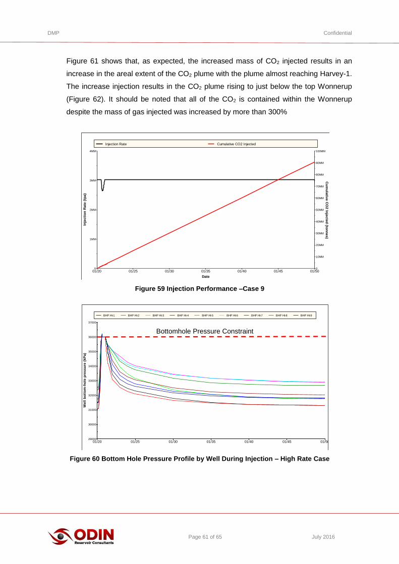
DMP Confidential

of 65 July 2016

Figure 61 shows that, as expected, the increased mass of CO2 injected results in an

increase in the areal extent of the CO2 plume with the plume almost reaching Harvey-1.

The increase injection results in the CO2 plume rising to just below the top Wonnerup

(Figure 62). It should be noted that all of the CO2 is contained within the Wonnerup

despite the mass of gas injected was increased by more than 300%

Figure 59 Injection Performance –Case 9

Figure 60 Bottom Hole Pressure Profile by Well During Injection – High Rate Case

01/20 01/25 01/30 01/35 01/40 01/45 01/50

Date

0

1MM

2MM

3MM

4MM

Inje

cti

on

Ra

te (

tpa

)

0

10MM

20MM

30MM

40MM

50MM

60MM

70MM

80MM

90MM

100MM

Cu

mu

lativ

e C

O2 In

jecte

d (to

nn

es)

Injection Rate Cumulative CO2 Injected

01/20 01/25 01/30 01/35 01/40 01/45 01/5029000

30000

31000

32000

33000

34000

35000

36000

37000

Well

bo

tto

m-h

ole

pre

ssu

re (

kP

a)

BHP HI-1 BHP HI-2 BHP HI-3 BHP HI-4 BHP HI-5 BHP HI-6 BHP HI-7 BHP HI-8 BHP HI-9

Bottomhole Pressure Constraint

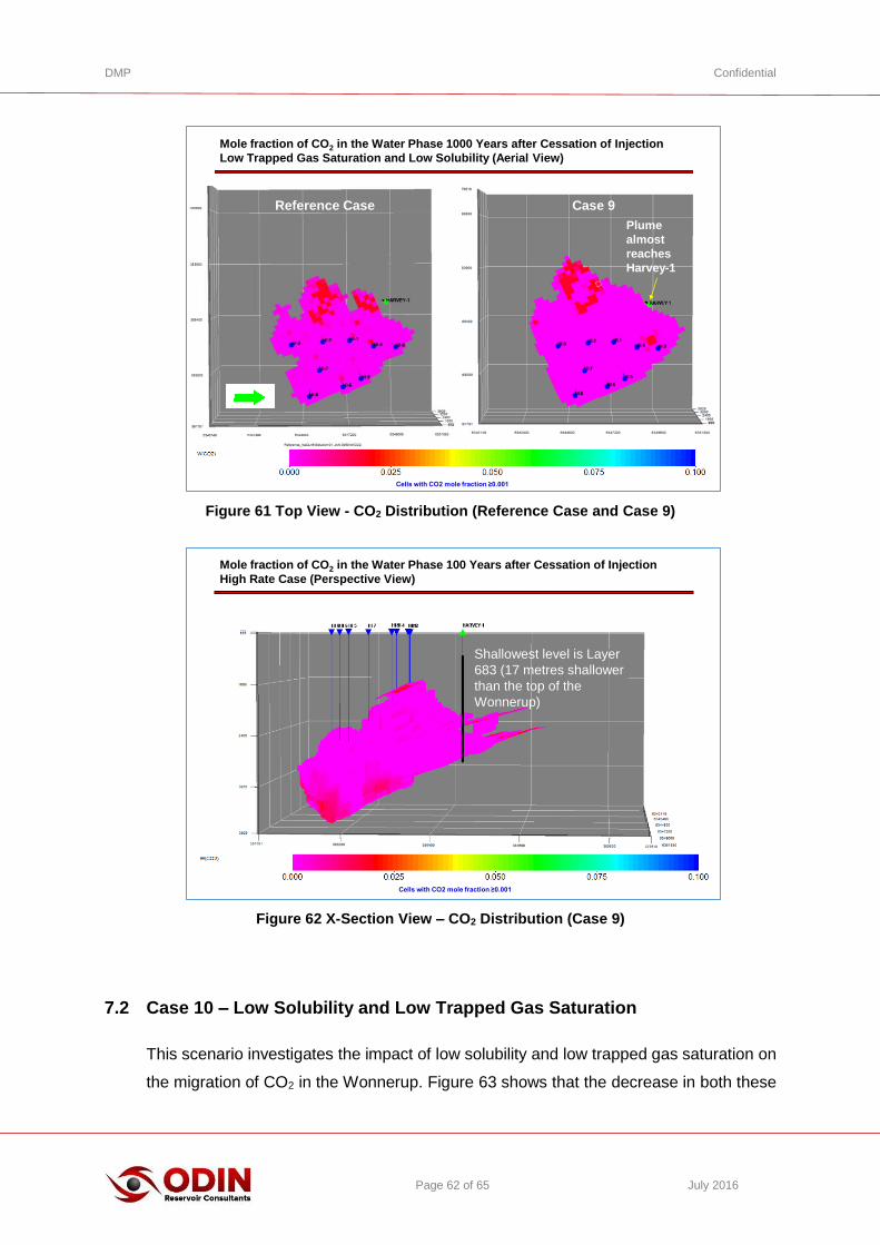
DMP Confidential

of 65 July 2016

Figure 61 Top View - CO2 Distribution (Reference Case and Case 9)


7.2 Case 10 – Low Solubility and Low Trapped Gas Saturation

This scenario investigates the impact of low solubility and low trapped gas saturation on

the migration of CO2 in the Wonnerup. Figure 63 shows that the decrease in both these

Page 102 Tel: +61-414-246-600


Low Trapped Gas Saturation and Low Solubility (Aerial View)

Plume

almost

reaches

Harvey-1


Case 9Reference Case

Page 100 Tel: +61-414-246-600


High Rate Case (Perspective View)


683 (17 metres shallower

than the top of the

Wonnerup)


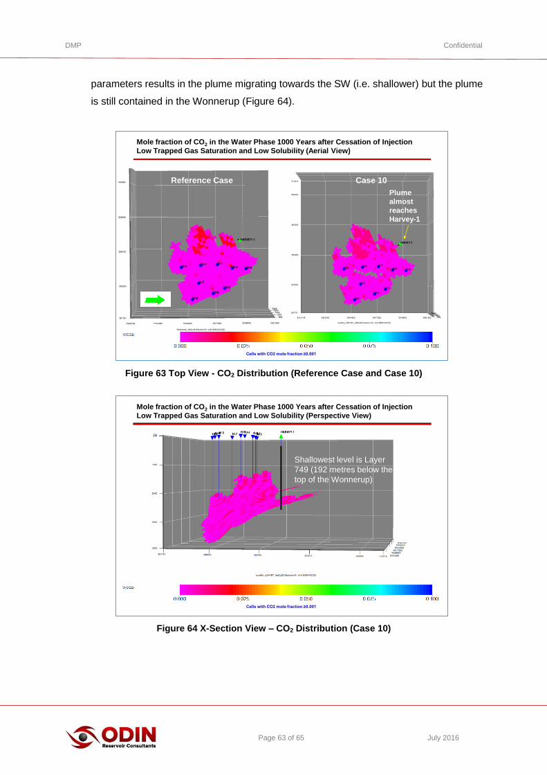
DMP Confidential

of 65 July 2016

parameters results in the plume migrating towards the SW (i.e. shallower) but the plume

is still contained in the Wonnerup (Figure 64).

Figure 63 Top View - CO2 Distribution (Reference Case and Case 10)


Page 102 Tel: +61-414-246-600


Low Trapped Gas Saturation and Low Solubility (Aerial View)

Plume

almost

reaches

Harvey-1


Case 10Reference Case

Page 103 Tel: +61-414-246-600


Low Trapped Gas Saturation and Low Solubility (Perspective View)





DMP Confidential

of 65 July 2016

8. FURTHER WORK

The results of the modelling show that it could be feasible to inject 800,000 tpa of CO2

over 30 years in the Yalgorup and Wonnerup formations in the Harvey area. Our

modelling studies show that all of the injected CO2 remains in the Wonnerup and that the

main factors controlling CO2 plume migration are trapped gas saturation and the solubility

of CO2 in brine. Uncertainties in end point relative permeability, vertical permeability or

the fraction of high energy facies in the Wonnerup are a second order effect. The study

also highlights the paucity of SCAL and water salinity data from the Harvey area which

can be used to further constrain the range of results from the simulation studies.

It is recommended that more SCAL data be obtained from the Harvey area. More data

is required in the following areas:

Steady state trapped gas saturation for High and Low Energy Facies.

Supercritical CO2 – water capillary pressure curves at reservoir conditions for High

and Low Energy facies.

Solubility and geochemical reaction data for CO2 and the formation brine.

ODIN also recommends that detailed fine grid simulations be conducted to examine the

impact of coarsening the grid in the lateral direction and also to calibrate the solubility of

CO2 in the coarse grid blocks.

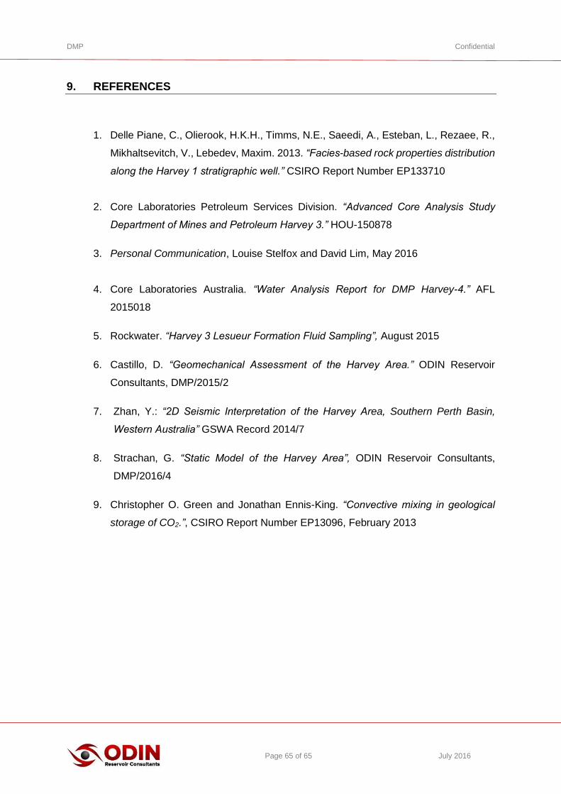
DMP Confidential

of 65 July 2016

9. REFERENCES

1. Delle Piane, C., Olierook, H.K.H., Timms, N.E., Saeedi, A., Esteban, L., Rezaee, R.,

Mikhaltsevitch, V., Lebedev, Maxim. 2013. “Facies-based rock properties distribution

along the Harvey 1 stratigraphic well.” CSIRO Report Number EP133710

2. Core Laboratories Petroleum Services Division. “Advanced Core Analysis Study

Department of Mines and Petroleum Harvey 3.” HOU-150878

3. Personal Communication, Louise Stelfox and David Lim, May 2016

4. Core Laboratories Australia. “Water Analysis Report for DMP Harvey-4.” AFL

2015018

5. Rockwater. “Harvey 3 Lesueur Formation Fluid Sampling”, August 2015

6. Castillo, D. “Geomechanical Assessment of the Harvey Area.” ODIN Reservoir

Consultants, DMP/2015/2

7. Zhan, Y.: “2D Seismic Interpretation of the Harvey Area, Southern Perth Basin,

Western Australia” GSWA Record 2014/7

8. Strachan, G. “Static Model of the Harvey Area”, ODIN Reservoir Consultants,

DMP/2016/4

9. Christopher O. Green and Jonathan Ennis-King. “Convective mixing in geological

storage of CO2.”, CSIRO Report Number EP13096, February 2013

department of mines and petroleum · dynamic modelling of co 2 sequestration in the harvey area a...

Documents