department of mathematics education, akenten appiah menka
TRANSCRIPT

Optimal control and comprehensive cost-effectiveness analysis for COVID-19
Joshua Kiddy Kwasi Asamoaha,b,∗, Eric Okyerec, Afeez Abidemid, Stephen E. Mooreg, Gui-QuanSuna,f,∗, Zhen Jina,b, Edward Acheampongg, Joseph Frank Gordonh
aComplex Systems Research Center, Shanxi University, Taiyuan 030006, PR ChinabShanxi Key Laboratory of Mathematical Techniques and Big Data Analysis on Disease Control and Prevention, Shanxi
University, Taiyuan 030006, PR ChinacDepartment of Mathematics and Statistics, University of Energy and Natural Resources, Sunyani, Ghana
dDepartment of Mathematical Sciences, Federal University of Technology Akure, PMB 704, Ondo State, NigeriaeDepartment of Mathematics, University of Cape Coast, Cape Coast, Ghana
fDepartment of Mathematics, North University of China, Taiyuan, Shanxi 030051, ChinagDepartment of Statistics and Actuarial Science University of Ghana, P.O. Box LG 115, Legon, Ghana
hDepartment of Mathematics Education, Akenten Appiah Menka University of Skills Training and EntrepreneurialDevelopment, Kumasi, Ghana
Abstract
Cost-effectiveness analysis is a mode of determining both the cost and economic health outcomes of one
or more control interventions. In this work, we have formulated a non-autonomous nonlinear determin-
istic model to study the control of COVID-19 to unravel the cost and economic health outcomes for the
autonomous nonlinear model proposed for the Kingdom of Saudi Arabia. The optimal control model
captures four time-dependent control functions, thus, u1-practising physical or social distancing proto-
cols; u2-practising personal hygiene by cleaning contaminated surfaces with alcohol-based detergents;
u3-practising proper and safety measures by exposed, asymptomatic and symptomatic infected individ-
uals; u4-fumigating schools in all levels of education, sports facilities, commercial areas and religious
worship centres. We proved the existence of the proposed optimal control model. The optimality system
associated with the non-autonomous epidemic model is derived using Pontryagin’s maximum principle.
We have performed numerical simulations to investigate extensive cost-effectiveness analysis for fourteen
optimal control strategies. Comparing the control strategies, we noticed that; Strategy 1 (practising
physical or social distancing protocols) is the most cost-saving and most effective control intervention in
Saudi Arabia in the absence of vaccination. But, in terms of the infection averted, we saw that strategy
6, strategy 11, strategy 12, and strategy 14 are just as good in controlling COVID-19.
Keywords: Control strategies; Existence of optimal control; Cost minimizing analysis, Economic health
outcomes.
∗Corresponding authorsEmail addresses: [email protected] (Joshua Kiddy Kwasi Asamoah), [email protected] ( Gui-Quan Sun)
Preprint submitted to xxxxx July 21, 2021
arX
iv:2
107.
0959
5v1
[m
ath.
OC
] 2
0 Ju
l 202
1

1. Introduction
The recent worldwide outbreaks of COVID-19 infectious disease has attracted a lot of attention in the
mathematical modelling and analysis of the COVID-19. In [1], the basic SEIR epidemic model is used to
study and explain some analytical results for the asymptotic and peak values and their characteristic times
of the susceptible human populations affected by the highly contagious COVID-19 disease. A SLIAR-type
epidemic model is used to study COVID-19 infections in China [2]. Estimated basic reproduction numbers
for the COVID-19 infectious disease transmission dynamics in Italy and China have been carried out in
[3], using a modified classical SIR mathematical model characterized by time-dependent transmission
rates. A prediction and data-driven based SEIRQ COVID-19 nonlinear infection model is formulated and
studied in [4]. The authors in [5] have developed and analyzed a nonlinear epidemic model to explain the
spreading dynamics of the 2019 coronavirus among the susceptible human population, the environment as
well as wild animals. Two novel data-driven compartmental models are proposed in [6, 7] to investigate
the COVID-19 pandemic in South Africa.
Mathematical modelling tools are essential in studying infectious diseases epidemiology because they
can at least give some insight into the spreading dynamics of disease outbreaks and help in suggesting
possible control strategies. The authors in [8] have constructed and analyzed a non-autonomous differential
equation model by introducing medical mask, isolation, treatment, and detergent spray as time-dependent
controls. Global parameter sensitivity analysis for a new COVID-19 differential equation model is carried
out in the work of Ali and co-authors [9]. They also proposed and analyzed a non-autonomous epidemic
model for the COVID-19 disease in the same work using quarantine and isolation as time-dependent
control functions. Furthermore, a COVID-19 mathematical is studied in recent work by the authors in [10],
where they considered three time-dependent control functions consisting of preventive control measures
(quarantine, isolation, social distancing), disinfection of contaminated surfaces to reduce intensive medical
care and infected individuals in the population. A non-optimal and optimal control deterministic COVID-
19 models are studied in [11]. The authors explored control and preventive interventions such as rapid
testing, medical masks, improvement of medical treatment in hospitals, and community awareness. An
optimal control nonlinear epidemic model for COVID-19 infection that captures optimal preventive and
control strategies such as personal protection measures, treatment of hospitalized individuals, and public
health education is formulated and analyzed to study the dynamics of the epidemic in Ethiopia [12].
Optimal Control analysis for the 2019 coronavirus epidemic has been studied using non-pharmaceutical
control and preventive interventions to examine the dynamics of the disease in the USA [13]. The work
in [14] studied a fractional-order mathematical model for COVID-19 dynamics with quarantine, isolation,
and environmental viral load. Asamoah et.al.[15] presented a COVID-19 model to study the impact
2

of the environment on the spread of the disease in Ghana. They further investigated the economic
outcomes using cost-effectiveness analysis. Alqarni [16] formulated and analyzed a novel deterministic
COVID-19 epidemic model characterized by nonlinear differential equations with six state variables to
describe the COVID-19 dynamics in the Kingdom of Saudi Arabia. They gave a detailed qualitative
stability analysis and also determined the influential model parameters on the basic reproduction number,
R0, using global sensitivity analysis. They further performed numerical simulations to support their
theoretical results, following their novel mathematical modelling formulation, analysis, and the generated
global sensitivity analysis results. We are motivated to present a cost-effectiveness analysis for the work
in [16]. In recent times, cost-effectiveness analysis of epidemic optimal control models has become very
important in suggesting realistic optimal control strategies to help reduce the spread of infectious diseases
in limited-resource settings. Also, assessing the amount it cost to acquire a unit of a health outcome like
infection averted, susceptibility prevented, life-year gained, or death prevented, and the expenses and well-
being results of at least one or more interventions. See, e.g., [17, 18, 19, 20, 21, 22, 23, 24, 25, 26, 27, 28,
29, 30, 31, 32, 33] and some of the references therein. There are vast area of research on COVID-19 where
author(s) did not either study optimal version of their proposed model or that of the economic impact
of their model see for example ([34, 35, 36, 37, 38, 39, 40, 41, 42, 43, 44, 45, 46, 47] e.t.c), therefore, we
hope that this article encourages researchers to dive deeper in investigating the economic-health impacts
of COVID-19 models without optimal control analysis and cost-effectiveness analysis as done in [48]. The
rest of the paper is organised as follows: Section 2 presents the general description of the model states,
and transition terms from Alqarni [16], Section 3 gives the bases for the formulation of the optimal control
model, the proof of existence and the characterisation of the optimal control problem. Section 4 contains
the numerical simulations for the various control strategies and cost-effectiveness analysis. Section 5
contain the concluding remarks.
2. The autonomous model
The formulated model is divided into five distinct human compartments, identified as, the susceptible,
S(t), exposed, E(t), asymptomatic infected (not showing symptoms but infected other healthy people)
A(t), symptomatic infected (that have symptoms of disease and infect other people) I(t), and the recovered
individuals, R(t), where the total population is given as N(t) = S(t) + E(t) + A(t) + I(t) + R(t). The
assumed concentration of the SARS-CoV-2 in the environment is denoted by B(t). Individuals in the
infected classes E(t), A(t), I(t) are assumed of transmitting the disease to the susceptible individuals at
the rate β1, β2, β3, respectively, and β4 is the propensity rate of susceptible individuals getting the virus
3

through the environment. The set of differential equations for the autonomous system is given as
dS
dt= Λ−
(β1E + β2I + β3A
) SN− β4B
S
N− dS,
dE
dt=(β1E + β2I + β3A
) SN
+ β4BS
N− (δ + d)E,
dI
dt= (1− τ)δE − (d+ d1 + γ1)I, (1)
dA
dt= τδE − (d+ γ2)A,
dR
dt= γ1I + γ2A− dR,
dB
dt= ψ1E + ψ2I + ψ3A− φB,
with the initial conditions
S(0) = S0 > 0, E(0) = E0 ≥ 0, I(0) = I0 ≥ 0, A(0) = A0 ≥ 0, R(0) = R0 ≥ 0, B(0) = B0 ≥ 0.
The model’s recruitment rate is given as Λ with d representing the natural death rate. The Greek symbols
β1, β2, β3, are the respective direct transmission rates among exposed and susceptible individuals, infected
(showing symptoms) and susceptible individuals, symptomatically infected (not showing symptoms) and
susceptible individuals, and β4 is the indirect transmission of the virus to the susceptible individuals.
The rate at which the exposed individuals develops symptoms become infected is denoted as (1 − τ)δ,
where the rate of new asymptomatic infection is represented as τδ. The disease-induced death rate is
denoted as d1. Here, the symptomatic, asymptomatic recovery rate is epidemiological assumed as γ1 and
γ2, respectively. Furthermore, the epidemiological rates for shedding the virus into the environment by
the exposed, infected and asymptomatically infected people is denoted as ψ1, ψ2 and ψ3 respectively. The
rate of natural removal of the virus from the environment is denoted as φ. Alqarni et.al[16] gave the
basic reproduction expression, detailed qualitative stability analysis and also determined the influential
model parameters on the basic reproduction number, R0, using global sensitivity analysis. They further
performed numerical simulations to support their theoretical results. The basic reproduction number
from Alqarni et.al[16] is given as
R0 =k2(δτ(β4ψ3 + β3φ) + k3(β4ψ1 + β1φ)) + δk3(1− τ)(β4ψ2 + β2φ)
k1k2k3φ, (2)
where k1 = d+ δ, k2 = γ1 + d+ d1 and k3 = γ2 + d. Following their global sensitivity result of the basic
reproduction number, section 3 is conceived.
3. Optimal control problem formulation and analysis of COVID-19 model
In section 4.1 of the work in Alqarni et al. [16]. They found out that the most sensitive parameters
in their basic reproduction number are: Contact rate among exposed and susceptible, β1, contact rate
4

among environment and susceptible, β4, virus contribution due to state E to compartment B, ψ1, and
virus removal from the environment, θ. Therefore, to contribute the research knowledge on COVID-19
in Saudi Arabia, we incorporated the following control terms to study the most effective economic and
health outcomes in combating this disease which has caused economic hardship in many countries.
3.1. Formulation of the non-autonomous COVID-19 model
• u1: practising physical or social distancing protocols.
• u2: practising personal hygiene by cleaning contaminated surfaces with alcohol based detergents.
• u3: practising proper and safety measures by exposed, asymptomatic infected and symptomatic
infected individuals.
• u4: fumigating schools in all levels of education, sports facilities, commercial areas and religious
worship centres.
Hence, based on [16], our optimal control model of is given as
dS
dt= Λ− (1− u1(t))
(β1E + β2I + β3A
) SN− (1− u1(t)− u2(t))β4B
S
N− dS,
dE
dt= (1− u1(t))
(β1E + β2I + β3A
) SN
+ (1− u1(t)− u2(t))β4BS
N− (δ + d)E,
dI
dt= (1− τ)δE − (d+ d1 + γ1)I, (3)
dA
dt= τδE − (d+ γ2)A,
dR
dt= γ1I + γ2A− dR,
dB
dt= (1− u3(t))ψ1E + (1− u3(t))ψ2I + (1− u3(t))ψ3A− (u4(t) + φ)B,
3.2. Formulation of the objective functional
In line with the standard in literature [15, 23, 24, 30, 49, 50, 51, 52, 53, 54], the control cost is measures
by implementing a quadratic performance index or objective functional in this work. Thus, our goal is to
minimize the objective functional, J , given as
J (u1, u2, u3, u4) := min
∫ T
0
[A1E +A2I +A3A+A4B +
1
2
4∑i=1
Diu2i (t)
]dt (4)
subject to the non-autonomous system (3), where Ai > 0 (i = 1, 2, 3, 4) are the balancing weight constants
on the exposed, asymptomatic and symptomatic infected individuals, and the concentration of corona
virus in the environment respectively, whereas Di > 0 are the balancing cost factors on the respective
controls ui (for i = 1, . . . , 4), T is the final time for controls implementation.
5

Suppose U is a non-empty control set defined by
U = {(u1, u2, u3, u4) : ui Lebesgue measurable, 0 ≤ ui ≤ 1, for i = 1, . . . , 4, t ∈ [0, T ]} . (5)
Then, it is of particular interest to seek an optimal control quadruple u∗ = (u∗1, u∗2, u∗3, u∗4) such that
J (u∗) = min {J (u1, u2, u3, u4) : u1, u2, u3, u4 ∈ U} . (6)
3.3. Existence of an optimal control
Theorem 3.1. Given the objective functional J defined on the control set U in (5), then there exists
an optimal control quadruple u∗ = (u∗1, u∗2, u∗3, u∗4) such that (6) holds when the following conditions are
satisfied [20, 29, 26]:
(i) The admissible control set U is convex and closed.
(ii) The state system is bounded by a linear function in the state and control variables.
(iii) The integrand of the objective functional J in (4) is convex in respect of the controls.
(iv) The Lagrangian is bounded below by
a0
(4∑i=1
|ui|2)a2
2
− a1,
where a0, a1 > 0 and a2 > 1.
Proof. Let the control set U = [0, umax]4, umax ≤ 1 , u = (u1, u2, u3, u4) ∈ U , x = (S,E, I, A,R,B) and
f0(t, x, u) be the right-hand side of the non-autonomous system (3) given by
f0(t, x, u) =
Λ− (1− u1) (β1E+β2I+β3A)SN − (1− u1 − u2)β4BSN − dS
(1− u1) (β1E+β2I+β3A)SN + (1− u1 − u2)β4BSN − (δ + d)E
(1− τ)δE − (d+ d1 + γ1)I
τδE − (d+ γ2)A
γ1I + γ2A− dR
(1− u3)ψ1E + (1− u3)ψ2I + (1− u3)ψ3A− (u4 + φ)B
. (7)
Then, we proceed by verifying the four properties presented by Theorem 3.1.
(i) Given the control set U = [0, umax]4. Then, by definition, U is closed. Further, let v, w ∈ U , where
v = (v1, v2, v3, v4) and w = (w1, w2, w3, w4), be any two arbitrary points. It then follows from the
definition of a convex set [55], that
λv + (1− λ)w ∈ [0, umax]4, for all λ ∈ [0, umax].
Consequently, λv + (1− λ)w ∈ U , implying the convexity of U .
6

(ii) This property is verified by adopting the ideas of the previous authors [26, 56]. Obviously, f0(t, x, u)
in (7) can be written as
f0(t, x, u) = f1(t, x) + f2(t, x)u,
where
f1(t, x) =
Λ− (β1E+β2I+β3A)SN − β4BS
N − dS(β1E+β2I+β3A)S
N + β4BSN − (δ + d)E
(1− τ)δE − (d+ d1 + γ1)I
τδE − (d+ γ2)A
γ1I + γ2A− dR
ψ1E + ψ2I + ψ3A− φB
and
f2(t, x) =
(β1E+β2I+β3A)SN + β4BS
Nβ4BSN 0 0
− (β1E+β2I+β3A)SN − β4BS
N −β4BSN 0 0
0 0 0 0
0 0 0 0
0 0 0 0
0 0 −(ψ1E + ψ2I + ψ3A) −B
.
Hence,
‖ f0(t, x, u) ‖ ≤‖ f1(t, x) ‖ +f2(t, x) ‖‖ u ‖
≤ b1 + b2 ‖ u ‖,
where b1 and b2 are positive constants given as
b1 =√
max {c1, c2} (Λ2 + Λ2(ψ1 + ψ2 + ψ3)2),
and
b2 =√
max {d1, d2} (Λ2 + Λ2(ψ1 + ψ2 + ψ3)2),
7

with
c0 = d2 + β3(2β1 + 2β2 + β3) + (β1 + β2)2 + (1− 2τ + 2τ2)δ2 + (γ1 + γ2)2 + ψ3(2ψ1 + 2ψ2 + ψ3)
+ (ψ1 + ψ2)2,
c1 =c0
d2,
c2 =2β4(β1φ+ β2φ+ β3φ) + β2
4(ψ1 + ψ2 + ψ3)
d2φ2(ψ1 + ψ2 + ψ3),
d1 =2β3(2β1 + 2β2 + β3) + 2(β1 + β2)2 + (ψ1 + ψ3)2 + ψ2(2ψ1 + ψ2 + 2ψ3)
d2,
d2 =4β4φ(β1 + β2 + β3) + (1 + 4β2
4)(ψ1 + ψ2 + ψ3)
d2φ2(ψ1 + ψ2 + ψ3).
(iii) First note that the objective functional J in (6) has an integrand of the Lagrangian form defined
as
L(t, x, u) = A1E +A2I +A3A+A4B =1
2
4∑i=1
Diu2i . (8)
Let v = (v1, v2, v3, v4) ∈ U , w = (w1.w2, w3, w4) ∈ U and λ ∈ [0, umax], then it suffices to prove that
L(t, x, (1− λ)v + λw) ≤ (1− λ)L(t, x, v) + λL(t, x, w). (9)
From (8),
L(t, x, (1− λ)v + λw) = A1E +A2I +A3A+A4B +1
2
4∑i=1
[Di((1− λ)vi + λwi)
2], (10)
and
(1− λ)L(t, x, v) + λL(t, x, w) = A1E +A2I +A3A+A4B+1
2(1− λ)
4∑i=1
Div2i +
1
2λ
4∑i=1
Diw2i . (11)
Applying the inequality (9) to the results in (10) and (11) leads to
L(t, x, (1−λ)v+λw)−((1−λ)L(t, x, v)+λL(t, x, w)) =1
2(λ2−λ)
4∑i=1
Di(vi−wi)2 ≤ 0, since λ ∈ [0, umax],
implying that the integrand L(t, x, u) of the objective functional J is convex.
(iv) Lastly, the fourth property is verified as follows:
L(t, x, u) = A1E +A2I +A3A+A4B =1
2
4∑i=1
Diu2i ,
≥ 1
2
4∑i=1
Diu2i ,
≥ a0
(|u1|2 + |u2|2 + |u3|2 + |u4|2
)a22 − a1,
where a0 = 12 max {D1, D2, D3, D4}, a1 > 0 and a2 = 2.
8

3.4. Characterization of the optimal controls
Pontryagin’s maximum principle (PMP) provides the necessary conditions that an optimal control
quadruple must satisfy. This principle converts the optimal control problem consisting of the non-
autonomous system (3) and the objective functional J in (4) into an issue of minimizing pointwise a
Hamiltonian, denoted as H, with respect to controls u = (u1, u2, u3, u4). First, the Hamiltonian H
associated with the optimal control problem is formulated as
H = A1E +A2I +A3A+A4B +1
2
(D1u
21 +D2u
22 +D3u
23 +D4u
24
)+ λ1
[Λ− (1− u1)
(β1E + β2I + β3A
) SN− (1− u1 − u2)β4B
S
N− dS
]+ λ2
[(1− u1)
(β1E + β2I + β3A
) SN
+ (1− u1 − u2)β4BS
N− (δ + d)E
]+ λ3
[(1− τ)δE − (d+ d1 + γ1)I
](12)
+ λ4
[τδE − (d+ γ2)A
]+ λ5
[γ1I + γ2A− dR
]+ λ6
[(1− u3)ψ1E + (1− u3)ψ2I + (1− u3)ψ3A− (u4 + φ)B
],
where λi (with i = 1, 2, . . . , 6) are the adjoint variables corresponding to the state variables S, E, I, A,
R and B respectively.
Theorem 3.2. If u∗ = (u∗i ), i = 1, . . . , 4 is an optimal control quadruple and S∗, E∗, I∗, A∗, R∗, B∗ are
the solutions of the corresponding state system (3) that minimizes J (u∗) over the control set U defined
9

by (5), then there exist adjoint variables λi (i = 1, 2, . . . , 6) satisfying
dλ1
dt= (λ1 − λ2)
[(1− u1)
(β1E
∗ + β2I∗ + β3A
∗)](E∗ + I∗ +A∗ +R∗)
N2
+ (λ1 − λ2)(1− u1 − u2)β4B∗ (E∗ + I∗ +A∗ +R∗)
N2+ λ1d,
dλ2
dt= −A1 + (λ1 − λ2)(1− u1)S∗
[(S∗ + I∗ +A∗ +R∗)β1 − (β2I
∗ + β3A∗)
N2
]+ (λ2 − λ1)(1− u1 − u2)β4B
∗ S∗
N2+ (δ + d)λ2 − λ2(1− τ)δλ3 − τδλ4 − (1− u3)ψ1λ6, (13)
dλ3
dt= −A2 + (λ1 − λ2)(1− u1)S∗
[(S∗ + E∗ +A∗ +R∗)β2 − (β1E
∗ + β3A∗)
N2
]+ (λ2 − λ1)(1− u1 − u2)β4B
∗ S∗
N2+ (δ + d1 + γ1)λ3 − γ1λ5 − (1− u3)ψ2λ6,
dλ4
dt= −A3 + (λ1 − λ2)(1− u1)S∗
[(S∗ + E∗ + I∗ +R∗)β3 − (β1E
∗ + β2I∗)
N2
]+ (λ2 − λ1)(1− u1 − u2)β4B
∗ S∗
N2+ (d1 + γ2)λ4 − γ2λ5 − (1− u3)ψ3λ6,
dλ5
dt= (λ2 − λ1)(1− u1)
(β1E
∗ + β2I∗ + β3A
∗)S∗
N2+ (λ2 − λ1)(1− u1 − u2)β4
S∗
N2+ λ5d,
dλ6
dt= −A4 + (λ1 − λ2)(1− u1 − u2)β4
S∗
N+ (u4 + φ)λ6d.
with transversality conditions
λi(T ) = 0, for i = 1, 2, . . . , 6 (14)
and
u∗1(t) = min
{max
{0,
(λ2 − λ1)(β1E∗ + β2I
∗ + β3A∗ + β4B
∗)S
D1N
}, u1max
},
u∗2(t) = min
{max
{0,
(λ2 − λ1)β4B∗S∗
D2N
}, u2max
},
u∗3(t) = min
{max
{0,λ6(ψ1E
∗ + ψ2I∗ + ψ3A
∗)
D3
}, u3max
},
u∗4(t) = min
{max
{0,φB∗λ6
D4
}, u4max
}.
(15)
Proof. The form of the adjoint system and the transversality conditions associated with this optimal
control problem follows the widely used standard results obtained from work done by Pontryagin et al.
[57]. For this purpose, we partially differentiate the formulated Hamiltonian function (12) with respect
10

to S,E, I, A,R and B as follows;
dλ1dt = −∂H
∂S , λ1(T ) = 0,
dλ2dt = −∂H
∂E , λ2(T ) = 0,
dλ3dt = −∂H
∂I , λ3(T ) = 0,
dλ4dt = −∂H
∂A , λ4(T ) = 0,
dλ3dt = −∂H
∂R , λ5(T ) = 0,
dλ4dt = −∂H
∂B , λ6(T ) = 0.
(16)
Finally, to obtain the desired results for the characterizations of the optimal control, we need to
partially differentiate the Hamiltonian function (12) with respect to the four time-dependent control
functions (u1, u2, u3, u4), thus, further, the optimal control characterization in (15) is obtained by solving
∂H∂ui
= 0, for u∗i (where i = 1, 2, 3, 4).
Lastly, it follows from standard control arguments involving bounds on the control that
u∗i =
0 if θ∗i ≤ 0,
θ∗i if 0 ≤ θ∗i ≤ umax,
umax if θ∗i ≥ umax,
where i = 1, 2, 3, 4 and with
θ1 =(λ2 − λ1)(β1E + β2I + β3A+ β4B)S
D1N,
θ2 =(λ2 − λ1)β4BS
D2N,
θ3 =λ6(ψ1E + ψ2I + ψ3A)
D3,
θ4 =φBλ6
D4.
4. Numerical simulation and cost-effectiveness analysis
4.1. Numerical simulation
Numerical simulations are vital in dynamical modelling; they give the proposed model’s pictorial view
to the theoretical analysis. Hence, we provide the numerical outcomes of our study by simulating 14
possible strategic combinations of the control measures. This is done by simulating the constraint system
11

(3) froward in time and the adjoint system (12) backward in time until convergence is reached. The
model parameters can be found in [16], but restated here for easy reference see Table 1. This simulation
procedure is popularly known as fourth-order Runge-Kutta forward-backward sweep simulations. The 14
possible strategic combination strategies are divided into four scenarios, thus, the implementation of single
control (Scenario A), the use of dual controls (Scenario B), the performance of triple controls (Scenario
C) and lastly, the implementation of quadruplet control measures (Scenario D). Iterated below as
♠ Scenario A (implementation of single control)
z Strategy 1: practising physical or social distancing protocols only
(u1 6= 0, u2 = u3 = u4 = 0).
z Strategy 2: practising personal hygiene by cleaning contaminated surfaces with alcohol based
detergents only (u1 = 0, u2 6= 0, u3 = u4 = 0).
z Strategy 3: practising proper and safety measures by exposed, asymptomatic infected and
symptomatic infected individuals only
(u1 = 0, u2 = 0, u3 6= 0, u4 = 0).
z Strategy 4: Fumigating schools in all levels of education, sports facilities, commercial areas
and religious worship centres only (u1 = 0, u2 = 0, u3 = 0, u4 6= 0).
♠ Scenario B (the use of double controls)
z Strategy 5: practising physical or social distancing protocols + practising personal hygiene by
cleaning contaminated surfaces with alcohol based detergents
(u1, u2 6= 0, u3 = u4 = 0).
z Strategy 6: practising physical or social distancing protocols + practising proper and safety
measures by exposed, asymptomatic infected and symptomatic infected individuals (u1, u3 6=
0, u2 = u4 = 0).
z Strategy 7: practising physical or social distancing protocols + fumigating schools in all levels
of education, sports facilities, commercial areas and religious worship centres (u1, u4 6= 0, u2 =
0, u3 = 0).
z Strategy 8: practising personal hygiene by cleaning contaminated surfaces with alcohol based
detergents + practising proper and safety measures by exposed, asymptomatic infected and
symptomatic infected individuals (u2, u3 6= 0, u1 = 0, u4 = 0).
12

z Strategy 9: practising personal hygiene by cleaning contaminated surfaces with alcohol based
detergents + fumigating schools in all levels of education, sports facilities, commercial areas
and religious worship centres (u2, u4 6= 0, u1 = 0, u3 = 0).
z Strategy 10: practising proper and safety measures by exposed, asymptomatic infected and
symptomatic infected individuals + fumigating schools in all levels of education, sports facili-
ties, commercial areas and religious worship centres (u3, u4 6= 0, u1 = 0, u2 = 0).
♠ Scenario C (the use of triple controls)
z Strategy 11: practising physical or social distancing protocols + practising personal hygiene
by cleaning contaminated surfaces with alcohol based detergents + practising proper and
safety measures by exposed, asymptomatic infected and symptomatic infected individuals
(u1, u2, u3 6= 0, u4 = 0).
z Strategy 12: practising physical or social distancing protocols + practising personal hygiene
by cleaning contaminated surfaces with alcohol based detergents + fumigating schools in all
levels of education, sports facilities, commercial areas and religious worship centres (u1, u2, u4 6=
0, u3 = 0).
z Strategy 13: practising personal hygiene by cleaning contaminated surfaces with alcohol based
detergents + practising proper and safety measures by exposed, asymptomatic infected and
symptomatic infected individuals + fumigating schools in all levels of education, sports facili-
ties, commercial areas and religious worship centres (u2, u3, u4 6= 0, u1 = 0).
♠ Scenario D (implementation of quadruplet)
z Strategy 14: practising physical or social distancing protocols + practising personal hygiene by
cleaning contaminated surfaces with alcohol based detergents + practising proper and safety
measures by exposed, asymptomatic infected and symptomatic infected individuals + fumigat-
ing schools in all levels of education, sports facilities, commercial areas and religious worship
centres (u1, u2, u3, u4 6= 0).
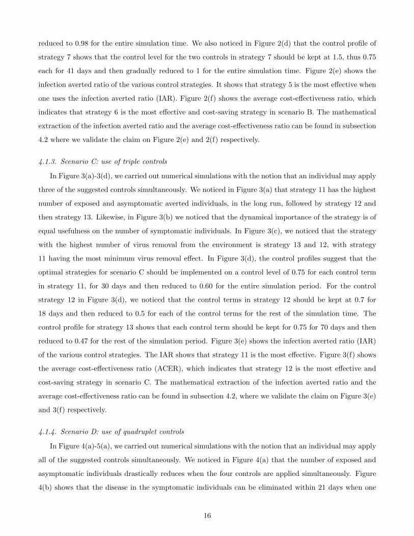
4.1.1. Scenario A: use of single control
In Figure 1(a), we noticed that strategy 1 has the highest number of exposed and asymptomatic
averted individuals, followed by strategy 4, strategy 3, and then strategy 1. Likewise, in Figure 1(b) we
noticed that the dynamical importance of the strategy is of equal usefulness on the number of symptomatic
individuals. In Figure 1(c), we saw that the strategy with the highest number of virus removal from the
13
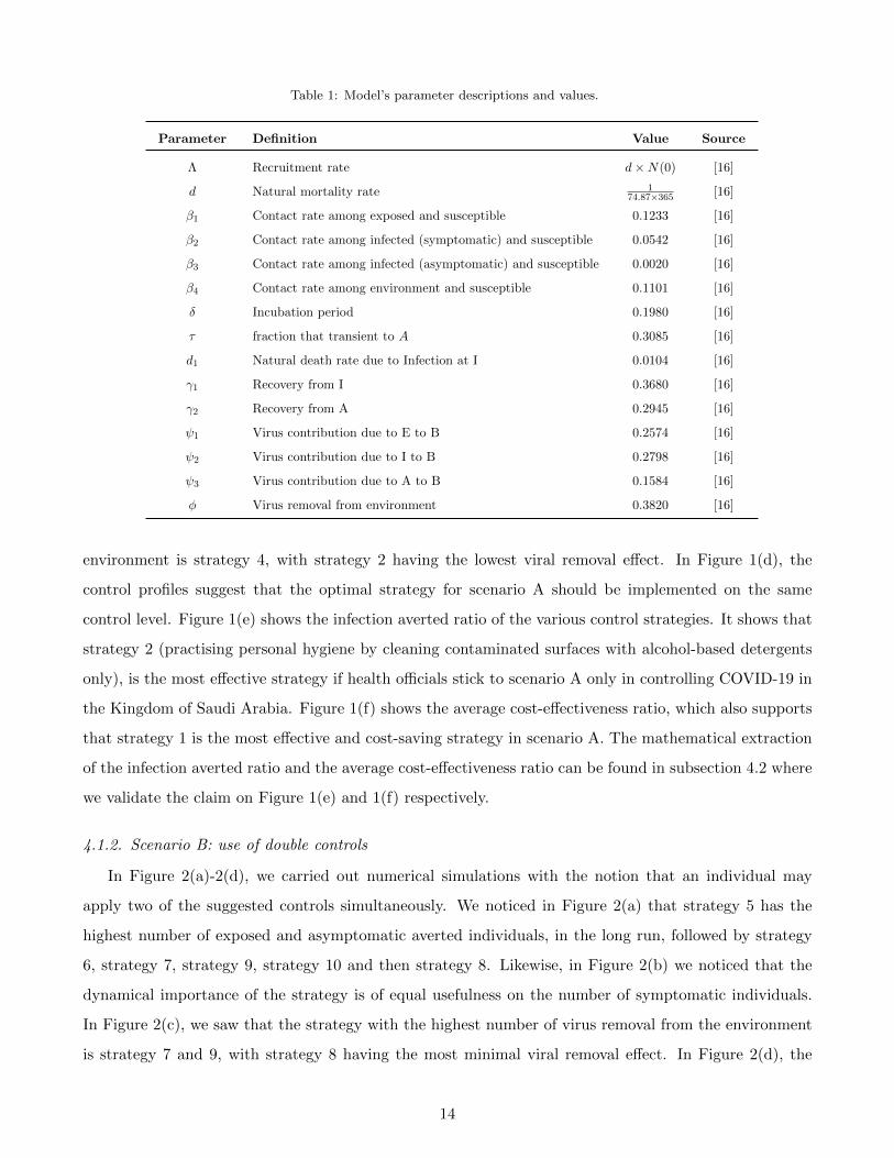
Table 1: Model’s parameter descriptions and values.
Parameter Definition Value Source
Λ Recruitment rate d×N(0) [16]
d Natural mortality rate 174.87×365 [16]
β1 Contact rate among exposed and susceptible 0.1233 [16]
β2 Contact rate among infected (symptomatic) and susceptible 0.0542 [16]
β3 Contact rate among infected (asymptomatic) and susceptible 0.0020 [16]
β4 Contact rate among environment and susceptible 0.1101 [16]
δ Incubation period 0.1980 [16]
τ fraction that transient to A 0.3085 [16]
d1 Natural death rate due to Infection at I 0.0104 [16]
γ1 Recovery from I 0.3680 [16]
γ2 Recovery from A 0.2945 [16]
ψ1 Virus contribution due to E to B 0.2574 [16]
ψ2 Virus contribution due to I to B 0.2798 [16]
ψ3 Virus contribution due to A to B 0.1584 [16]
φ Virus removal from environment 0.3820 [16]
environment is strategy 4, with strategy 2 having the lowest viral removal effect. In Figure 1(d), the
control profiles suggest that the optimal strategy for scenario A should be implemented on the same
control level. Figure 1(e) shows the infection averted ratio of the various control strategies. It shows that
strategy 2 (practising personal hygiene by cleaning contaminated surfaces with alcohol-based detergents
only), is the most effective strategy if health officials stick to scenario A only in controlling COVID-19 in
the Kingdom of Saudi Arabia. Figure 1(f) shows the average cost-effectiveness ratio, which also supports
that strategy 1 is the most effective and cost-saving strategy in scenario A. The mathematical extraction
of the infection averted ratio and the average cost-effectiveness ratio can be found in subsection 4.2 where
we validate the claim on Figure 1(e) and 1(f) respectively.
4.1.2. Scenario B: use of double controls
In Figure 2(a)-2(d), we carried out numerical simulations with the notion that an individual may
apply two of the suggested controls simultaneously. We noticed in Figure 2(a) that strategy 5 has the
highest number of exposed and asymptomatic averted individuals, in the long run, followed by strategy
6, strategy 7, strategy 9, strategy 10 and then strategy 8. Likewise, in Figure 2(b) we noticed that the
dynamical importance of the strategy is of equal usefulness on the number of symptomatic individuals.
In Figure 2(c), we saw that the strategy with the highest number of virus removal from the environment
is strategy 7 and 9, with strategy 8 having the most minimal viral removal effect. In Figure 2(d), the
14

0 20 40 60 80 100Time (days)
0
200
400
600
800
1000
1200
1400Ex
pose
d +
Asym
ptom
atic
indi
vidua
lsStrategy 1Strategy 2Strategy 3Strategy 4
Scenario A
(a)
0 20 40 60 80 100Time (days)
0
100
200
300
400
500
Sym
ptom
atic
indi
vidua
ls
Strategy 1Strategy 2Strategy 3Strategy 4
Scenario A
(b)
0 20 40 60 80 100Time (days)
0
1000
2000
3000
4000
5000
6000
Viru
s in
the e
nviro
nmen
t Strategy 1Strategy 2Strategy 3Strategy 4
Scenario A
(c)
0 20 40 60 80 100Time (days)
0
0.1
0.2
0.3
0.4
0.5
0.6
0.7
0.8
Cont
rol P
rofil
e Strategy 1Strategy 2Strategy 3Strategy 4
Scenario A
(d) Control profile
1 2 3 4
Strategies
0
0.2
0.4
0.6
0.8
1
1.2
1.4
1.6
Infe
ctio
n av
erte
d Ra
tio Scenario A
(e) Infection Averted Ratio
1 2 3 4Strategies
0
0.2
0.4
0.6
0.8
1
1.2
1.4
1.6
Aver
age C
ost-E
ffect
ivene
ss R
atio
10-3
Scenario A
(f) Average Cost-Effectiveness Ratio
Fig. 1: Single control strategy.
control profiles suggest that the optimal strategy for scenario B should be implemented on a control level
of 0.75 for each control term in strategy 5 and 8 for the entire simulation period. For the control strategy
9 in Figure 2(d), we noticed that the control terms in strategy 9, should be kept at 0.75 for 95 days and
then reduced to 0.5 for each of the control terms for the rest of the simulation time. The control profile
for strategy 10 shows that each control term should be kept for 0.75 for 92 days and then reduced to 0.5
for the rest of the simulation period. The control profile for strategy 6 shows that, with the combined
effort of the two controls, the strategy control level should be kept at 1.5 for 65 days and then gradually
15
reduced to 0.98 for the entire simulation time. We also noticed in Figure 2(d) that the control profile of
strategy 7 shows that the control level for the two controls in strategy 7 should be kept at 1.5, thus 0.75
each for 41 days and then gradually reduced to 1 for the entire simulation time. Figure 2(e) shows the
infection averted ratio of the various control strategies. It shows that strategy 5 is the most effective when
one uses the infection averted ratio (IAR). Figure 2(f) shows the average cost-effectiveness ratio, which
indicates that strategy 6 is the most effective and cost-saving strategy in scenario B. The mathematical
extraction of the infection averted ratio and the average cost-effectiveness ratio can be found in subsection
4.2 where we validate the claim on Figure 2(e) and 2(f) respectively.
4.1.3. Scenario C: use of triple controls
In Figure 3(a)-3(d), we carried out numerical simulations with the notion that an individual may apply
three of the suggested controls simultaneously. We noticed in Figure 3(a) that strategy 11 has the highest
number of exposed and asymptomatic averted individuals, in the long run, followed by strategy 12 and
then strategy 13. Likewise, in Figure 3(b) we noticed that the dynamical importance of the strategy is of
equal usefulness on the number of symptomatic individuals. In Figure 3(c), we noticed that the strategy
with the highest number of virus removal from the environment is strategy 13 and 12, with strategy
11 having the most minimum virus removal effect. In Figure 3(d), the control profiles suggest that the
optimal strategies for scenario C should be implemented on a control level of 0.75 for each control term
in strategy 11, for 30 days and then reduced to 0.60 for the entire simulation period. For the control
strategy 12 in Figure 3(d), we noticed that the control terms in strategy 12 should be kept at 0.7 for
18 days and then reduced to 0.5 for each of the control terms for the rest of the simulation time. The
control profile for strategy 13 shows that each control term should be kept for 0.75 for 70 days and then
reduced to 0.47 for the rest of the simulation period. Figure 3(e) shows the infection averted ratio (IAR)
of the various control strategies. The IAR shows that strategy 11 is the most effective. Figure 3(f) shows
the average cost-effectiveness ratio (ACER), which indicates that strategy 12 is the most effective and
cost-saving strategy in scenario C. The mathematical extraction of the infection averted ratio and the
average cost-effectiveness ratio can be found in subsection 4.2, where we validate the claim on Figure 3(e)
and 3(f) respectively.
4.1.4. Scenario D: use of quadruplet controls
In Figure 4(a)-5(a), we carried out numerical simulations with the notion that an individual may apply
all of the suggested controls simultaneously. We noticed in Figure 4(a) that the number of exposed and
asymptomatic individuals drastically reduces when the four controls are applied simultaneously. Figure
4(b) shows that the disease in the symptomatic individuals can be eliminated within 21 days when one
16

0 20 40 60 80 100Time (days)
0
100
200
300
400
500
600
700
800Ex
pose
d + A
sym
ptom
atic
indi
vidua
ls Strategy 5Strategy 6Strategy 7Strategy 8Strategy 9Strategy 10
Scenario B
(a)
0 20 40 60 80 100Time (days)
0
100
200
300
400
500
Sym
ptom
atic
indi
vidua
ls
Strategy 5Strategy 6Strategy 7Strategy 8Strategy 9Strategy 10
Scenario B
(b)
0 20 40 60 80 100Time (days)
0
1000
2000
3000
4000
5000
6000
Viru
s in
the e
nviro
nmen
t
Strategy 5Strategy 6Strategy 7Strategy 8Strategy 9Strategy 10
Scenario B
(c)
0 20 40 60 80 100Time (days)
0
0.5
1
1.5
Cont
rol P
rofil
e
Strategy 5Strategy 6Strategy 7Strategy 8Strategy 9Strategy 10 Scenario B
(d) Control profile
5 6 7 8 9 10Strategies
0
0.2
0.4
0.6
0.8
1
1.2
1.4
1.6
Infe
ctio
n av
erte
d Ra
tio
Scenario B
(e) Infection Averted Ratio
5 6 7 8 9 10Strategies
0
0.5
1
1.5
2
2.5
Aver
age C
ost-E
ffect
ivene
ss R
atio 10-3
Scenario B
(f) Average Cost-Effectiveness Ratio
Fig. 2: Double control strategies.
chooses to implement all the controls simultaneously. Figure 4(c) shows that the virus in the environment
can be eliminated within 10 days when one chooses to implement all the controls simultaneously. In
Figure 5(a) we showed the dynamical changes of each control considered in this work. We noticed that, in
the pool of the four controls, control u1 (practising physical or social distancing protocols) and control u2
(practising personal hygiene by cleaning contaminated surfaces with alcohol-based detergents) should be
applied at a constant level throughout, with much effort placed on control u1 for 98 days. For the control
u3 in Figure 5(a), we noticed that the control should be kept at 0.75 for 25 days and then gradually
17

0 20 40 60 80 100Time (days)
0
100
200
300
400
500Ex
pose
d + A
sym
ptom
atic
indi
vidua
lsStrategy 11Strategy 12Strategy 13
Scenario C
(a)
0 20 40 60 80 100Time (days)
0
100
200
300
400
500
Sym
ptom
atic
indi
vidua
ls Strategy 11Strategy 12Strategy 13
Scenario C
(b)
0 20 40 60 80 100Time (days)
0
1000
2000
3000
4000
5000
6000
Viru
s in
the e
nviro
nmen
t
Strategy 11Strategy 12Strategy 13
Scenario C
(c)
0 20 40 60 80 100Time (days)
0.5
1
1.5
2
2.5
Cont
rol P
rofil
eStrategy 11Strategy 12Strategy 13
Scenario C
(d) Control profile
11 12 13Strategies
0
0.2
0.4
0.6
0.8
1
1.2
1.4
1.6
Infe
ctio
n av
erte
d Ra
tio
Scenario C
(e) Infection Averted Ratio
11 12 13Strategies
0
0.5
1
1.5
2
2.5
Aver
age C
ost-E
ffect
ivene
ss R
atio 10-3
Scenario C
(f) Average Cost-Effectiveness Ratio
Fig. 3: Implementation of quadruplet controls.
reduced to 0.29 for the rest of the simulation time. The control profile for control u4 shows that the
control term should be kept for 0.75 for 18 days and then gradually reduced to 0.29 for the rest of the
simulation period. Finally, Figure 5(b) shows the efficacies plot for the number of exposed, asymptomatic,
symptomatic individuals and the number of viruses removed from the environment, respectively, when one
uses all the proposed control simultaneously. We noticed from the efficacies plot that the controls are more
efficient on the number of viral removed from the environment, followed by the number of symptomatic
individuals, asymptomatic individuals, and exposed individuals. The efficacy plots are obtained from
18

0 20 40 60 80 100Time (days)
0
500
1000
1500
2000Ex
pose
d +
Asym
ptom
atic
indi
vidua
ls
Without control measuresWith control measures
(a)
0 20 40 60 80 100Time (days)
0
100
200
300
400
500
600
Sym
ptom
atic
indi
vidua
ls
Without control measuresWith control measures
(b)
0 20 40 60 80 100Time (days)
0
1000
2000
3000
4000
5000
6000
Viru
s in
the e
nviro
nmen
t Without control measuresWith control measures
(c)
Fig. 4: With and without control strategies.
using the following functions:
EE =E(0)− E∗(t)
E(0), EI =
I(0)− I∗(t)I(0)
, EA =A(0)−A∗(t)
A(0), EB =
B(0)−B∗(t)B(0)
where E(0), I(0), A(0), B(0) are the initial data and E∗(t), I∗(t), A∗(t), B∗(t) are the function relating to
the “optimal states associated” with the controls [58]. Figure 5(b) shows that the controls attain 100%
efficacy on the disease induced compartment after 39 days.
0 20 40 60 80 100Time (days)
0
0.1
0.2
0.3
0.4
0.5
0.6
0.7
0.8
Cont
rol P
rofil
e
u1
u2
u3
u4
(a) Control profile
0 20 40 60 80 100Time (days)
0
0.2
0.4
0.6
0.8
1
Effic
acies
plo
t
EFE
EFI
EFA
EFB
(b) Efficacies ratio
Fig. 5: With and without control strategies.
19

4.2. Cost-effectiveness analysis
Given the four different scenarios considered for the implementation of optimal control problem in
section 4.1, cost-effectiveness analysis is employed to decide on the most cost-effective control intervention
strategy from other strategies for each of scenarios A–D, under investigation. To implement the cost-
effectiveness analysis, we use three approaches. These are: infection averted ratio (IAR) [23], average
cost-effectiveness ratio (ACER) and incremental cost-effectiveness ratio (ICER) [23, 48, 58]. Definitions
of the three approaches are given as follows:
Infection averted ratio (IAR)
Infection averted ratio (IAR) can be expressed as
IAR =Number of infections averted
Number of individuals recovered from the infection,
where the number of infections averted represents the difference between the total number of infected
individuals without any control implementation and the total number of infected individuals with control
throughout the simulation, a control strategy with the highest IAR value is considered as the most cost-
effective [23, 20, 48].
Average cost-effectiveness ratio (ACER)
Average cost-effectiveness ratio (ACER) is stated as
ACER =Total cost incurred on the implementation of a particular intervention strategy
Total number of infections averted by the intervention strategy.
The total cost incurred on implementing a particular intervention strategy is estimated from
C(u) =1
2
∫ T
0
4∑i=1
Diu2i dt. (17)
Incremental cost-effectiveness ratio (ICER)
Usually, the incremental cost-effectiveness ratio (ICER) measures the changes between the costs and
health benefits of any two different intervention strategies competing for the same limited resources.
Considering strategies p and q as two competing control intervention strategies, then ICER is stated as
ICER =Change in total costs in strategies p and q
Change in control benefits in strategies p and q.
ICER numerator includes the differences in disease averted costs, costs of prevented cases, intervention
costs, among others. While the denominator of ICER accounts for the differences in health outcome,
including the total number of infections averted or the total number of susceptibility cases prevented.
20

4.2.1. Scenario A: use of single control
Owing to the simulated results of the optimality system under scenario A (when only one control is
implemented with considerations of strategies 1–4) as shown in Figure 1, we calculate IAR, ACER and
ICER for each of the four control strategies.
For IAR, the fourth column of Table 2 summarizes the calculated values for the implemented strategies.
Accordingly, strategy 2 (practising personal hygiene by cleaning contaminated surfaces with alcohol-
based detergents only) has the highest IAR value, followed by strategy 1 (practising physical or social
distancing protocol only), strategy 4 (fumigating schools in all levels of education, sports facilities and
commercial areas such as markets and public toilet facilities only), and lastly strategy 3 (practising proper
and safety measures by the exposed, asymptomatic infected and symptomatic infected individuals only).
Consequently, the most cost-effective strategy according to this cost-effectiveness analysis approach is
strategy 2. The next most cost-effective strategy is strategy 1, followed by strategy 4, then strategy 3.
According to the ACER cost-effectiveness analysis method, strategy 4 has the highest ACER value,
followed by strategy 3, strategy 2 and strategy 1 as shown in the fifth column of Table 2. Therefore,
the cost-effectiveness of the four strategies implemented, ranging from the most cost-effective to the least
cost-effective strategy, is given as strategy 1, strategy 2, strategy 3, and strategy 4.
Next, ICER values are computed for the four control intervention strategies under scenario A to
further affirm the most economical strategy among them. Based on the results obtained for the numerical
simulations of optimal control problem in scenario A (see Figure 1), strategies 1–4 are ranked according
to their increasing order in respect of the total number of COVID-19 infections averted in the community.
We have that Strategy 3 averts the least number of the disease infections, followed by Strategy 2, Strategy
4 and Strategy 1 as shown in Table 2.
Table 2: Incremental cost-effectiveness ratio for scenario A
Strategy Infection averted Cost IAR ACER ICER
Strategy 3: u3(t) 1.4423× 10⁶ 1.4063× 10³ 1.2325 9.7498× 10⁻⁴ 9.7498× 10⁻⁴
Strategy 2: u2(t) 1.6603× 10⁶ 1.4077× 10³ 1.5835 8.4784× 10⁻⁴ 6.4220× 10⁻⁶
Strategy 4: u4(t) 1.8000× 10⁶ 2.8098× 10³ 1.2914 0.0016 0.0100
Strategy 1: u1(t), 2.0679× 10⁶ 281.1135 1.5793 1.3594× 10⁻⁴ −0.0004
Thus, ICER is computed for the competing control Strategy 1, Strategy 2, Strategy 3 and Strategy 4
21
as follows:
ICER(3) =1.4063× 10³ − 0
1.4423× 10⁶ − 0= 9.7504× 10⁻⁴,
ICER(2) =1.4077× 10³ − 1.4063× 10³
1.6603× 10⁶ − 1.4423× 106= 6.4220× 10⁻⁶,
ICER(4) =2.8098× 10³ − 1.4077× 10³
1.8000× 10⁶ − 1.6603× 106= 0.0100,
ICER(1) =281.1135− 2.8098× 10³
2.0679× 10⁶ − 1.8000× 106= −0.0004.
The computed results (as presented in Table 2) indicate that the ICER value of Strategy 4, ICER(4), is
higher than that of Strategy 3. This means that the singular application of control u4 (fumigating schools
in all levels of education, sports facilities and commercial areas such as markets and public toilet facilities)
is more costly and less effective than when only control u3 (practising proper and safety measures by the
exposed, asymptomatic infected and symptomatic infected individuals) is applied. Thus, Strategy 4 is
eliminated from the list of alternative control strategies.
Then, ICER is further calculated for the competing Strategy 3 with Strategies 1 and 2. The compu-
tation is as follows:
ICER(3) =1.4063× 10³ − 0
1.4423× 10⁶ − 0= 9.7504× 10⁻⁴,
ICER(2) =1.4077× 10³ − 1.4063× 10³
1.6603× 10⁶ − 1.4423× 106= 6.4220× 10⁻⁶,
ICER(1) =281.1135− 1.4077× 10³
2.0679× 10⁶ − 1.6603× 106= −0.0028.
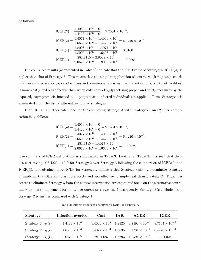
The summary of ICER calculations is summarized in Table 3. Looking at Table 3, it is seen that there
is a cost-saving of 6.4220× 10⁻⁶ for Strategy 2 over Strategy 3 following the comparison of ICER(2) and
ICER(3). The obtained lower ICER for Strategy 2 indicates that Strategy 3 strongly dominates Strategy
2, implying that Strategy 3 is more costly and less effective to implement than Strategy 2. Thus, it is
better to eliminate Strategy 3 from the control intervention strategies and focus on the alternative control
interventions to implement for limited resources preservation. Consequently, Strategy 3 is excluded, and
Strategy 2 is further compared with Strategy 1.
Table 3: Incremental cost-effectiveness ratio for scenario A
Strategy Infection averted Cost IAR ACER ICER
Strategy 3: u3(t) 1.4423× 10⁶ 1.4063× 10³ 1.2325 9.7498× 10⁻⁴ 9.7504× 10⁻⁴
Strategy 2: u2(t) 1.6603× 10⁶ 1.4077× 10³ 1.5835 8.4784× 10⁻⁴ 6.4220× 10⁻⁶
Strategy 1: u1(t), 2.0679× 10⁶ 281.1135 1.5793 1.3594× 10⁻⁴ −0.0028
22

We now face the re-calculation of the ICER for Strategies 1 and 2. The calculations are made as
follows:
ICER(2) =1.4077× 10³ − 0
1.6603× 10⁶ − 0= 8.4784× 10⁻⁴,
ICER(1) =281.1135− 1.4077× 10³
2.0679× 10⁶ − 1.6603× 106= −0.0028.
The results obtained from ICER computations are presented in Table 4. From Table 4, it is shown
that ICER(2) is greater than ICER(1). The implication of the lower ICER value obtained for Strategy
1 is that Strategy 2 strongly dominates, implying that Strategy 2 is more costly and less effective to
implement than Strategy 1. Therefore, Strategy 1 (practising physical or social distancing protocol only)
is considered the most cost-effective among the four strategies in Scenario A analysed in this work, which
confirms the results in Figure 1(f).
Table 4: Incremental cost-effectiveness ratio for scenario A
Strategy Infection averted Cost IAR ACER ICER
Strategy 2: u2(t) 1.6603× 10⁶ 1.4077× 10³ 1.5835 8.4784× 10⁻⁴ 8.4784× 10⁻⁴
Strategy 1: u1(t), 2.0679× 10⁶ 281.1135 1.5793 1.3594× 10⁻⁴ −0.0028
4.2.2. Scenario B: use of double controls
According to the results obtained from the numerical implementation of the optimality system under
Scenario B (when only two different controls are implemented with considerations of Strategies 5–10) as
illustrated in Figure 2, we discuss the IAR, ACER and ICER cost analysis techniques for Strategies 5–10
here.
To compare Strategies 5–10 using the IAR cost analysis approach, the computed values for the six
control strategies are as presented in the fourth column of Table 5. A look at Table 5 shows that Strategy
5 has the highest IAR. This is followed by Strategy 6, then Strategies 8, 7, 9 and 10. Therefore, it follows
that Strategy 5 (which combines practising physical or social distancing protocols with practising personal
hygiene by cleaning contaminated surfaces with alcohol-based detergents) is considered most cost-effective
among the six strategies in Scenario B as analysed according to the IAR cost analysis technique.
Also, we use the ACER technique to determine the most cost-effective strategy among the various
intervention strategies considered in Scenario B. From the results obtained (as shown contained in the
fifth column of Table 5), it is clear that Strategy 6 has the least ACER value, followed by Strategies 5,
7, 8, 9 and 10. Hence, Strategy 6 (which combines practising physical or social distancing protocols with
practising proper and safety measures by exposed, asymptomatic infected and asymptomatic infected
23

individuals) is the most cost-effective among the set of control strategies considered in Scenario B based
on the ACER cost-effective analysis method.
To further affirm the most cost-effective strategy among Strategies 5–10, we implement ICER cost
analysis approach on the six intervention strategies. Using the simulated results (as demonstrated in
Figure 2), the six control strategies are ranked from least to most effective according to the number of
COVID-19 infections averted as shown in Table 5. So, Strategy 8 averts the least number of infections,
followed by Strategy 10, Strategy 9, Strategy 6, Strategy 7 and Strategy 5, averting the most number of
infections in the population.
Table 5: Incremental cost-effectiveness ratio for scenario B
Strategy Infection averted Cost IAR ACER ICER
Strategy 8: u2(t), u3(t) 1.9253× 10⁶ 2.8104× 10³ 1.4524 0.0015 0.0015
Strategy 10: u3(t), u4(t) 1.9809× 10⁶ 4.1019× 10³ 1.3350 0.0021 0.0232
Strategy 9: u2(t), u4(t) 2.0684× 10⁶ 4.1495× 10³ 1.4077 0.0020 5.4400× 10⁻⁴
Strategy 6: u1(t), u3(t) 2.1128× 10⁶ 1.3487× 10³ 1.5239 6.3834× 10⁻⁴ −0.0631
Strategy 7: u1(t), u4(t) 2.1751× 10⁶ 1.7708× 10³ 1.4506 8.1410× 10⁻⁴ 0.0068
Strategy 5: u1(t), u2(t) 2.2265× 10⁶ 1.6871× 10³ 1.5759 7.5775× 10⁻⁴ −0.0016
The ICER value for each strategy is computed as follows:
ICER(8) =2.8104× 10³ − 0
1.9253× 10⁶ − 0= 0.0015,
ICER(10) =4.1019× 10³ − 2.8104× 10³
1.9809× 10⁶ − 1.9253× 106= 0.0232,
ICER(9) =4.1495× 10³ − 4.1019× 10³
2.0684× 10⁶ − 1.9809× 106= 5.4400× 10⁻⁴,
ICER(6) =1.3487× 10³ − 4.1495× 10³
2.1128× 10⁶ − 2.0684× 106= −00631,
ICER(7) =1.7708× 10³ − 1.3487× 10³
2.1751× 10⁶ − 2.1128× 106= 0.0068,
ICER(5) =1.6871× 10³ − 1.7708× 10³
2.2265× 10⁶ − 2.1751× 106= −0.0016.
From Table 5, it is observed that there is a cost-saving of $0.0068 for Strategy 7 over Strategy 10. This
follows the comparison of ICER(7) and ICER(10). The indication of the lower ICER value obtained
for Strategy 7 is that Strategy 10 strongly dominates Strategy 7. By implication, Strategy 10 is more
costly and less effective to implement when compared with Strategy 7. Therefore, it is better to exclude
Strategy 10 from the set of alternative intervention strategies. At this point, Strategy 7 is compared with
Strategies 5, 6, 8 and 9.
24

The ICER is computed as
ICER(8) =2.8104× 10³ − 0
1.9253× 10⁶ − 0= 0.0015,
ICER(9) =4.1495× 10³ − 2.8104× 10³
2.0684× 10⁶ − 1.9253× 106= 0.0094,
ICER(6) =1.3487× 10³ − 4.1495× 10³
2.1128× 10⁶ − 2.0684× 106= −00631,
ICER(7) =1.7708× 10³ − 1.3487× 10³
2.1751× 10⁶ − 2.1128× 106= 0.0068,
ICER(5) =1.6871× 10³ − 1.7708× 10³
2.2265× 10⁶ − 2.1751× 106= −0.0016.
The results obtained are summarized in Table 6. Table 6 shows a cost-saving of $0.0068 for Strategy 7 over
Table 6: Incremental cost-effectiveness ratio for scenario B
Strategy Infection averted Cost IAR ACER ICER
Strategy 8: u2(t), u3(t) 1.9253× 10⁶ 2.8104× 10³ 1.4524 0.0015 0.0015
Strategy 9: u2(t), u4(t) 2.0684× 10⁶ 4.1495× 10³ 1.4077 0.0020 0.0094
Strategy 6: u1(t), u3(t) 2.1128× 10⁶ 1.3487× 10³ 1.5239 6.3834× 10⁻⁴ −0.0631
Strategy 7: u1(t), u4(t) 2.1751× 10⁶ 1.7708× 10³ 1.4506 8.1410× 10⁻⁴ 0.0068
Strategy 5: u1(t), u2(t) 2.2265× 10⁶ 1.6871× 10³ 1.5759 7.5775× 10⁻⁴ −0.0016
Strategy 9 by comparing ICER(7) and ICER(9). The higher ICER value obtained for Strategy 9 implies
that Strategy 9 strongly dominated, more costly and less effective to implement when compared with
Strategy 7. Therefore, Strategy 9 is left out of the list of alternative control interventions to implement
for the purpose of preserving the limited resources. We further compare Strategy 7 with Strategies 5, 6
and 8.
The computation of ICER for Strategies 5, 6, 7 and 8 is as follows:
ICER(8) =2.8104× 10³ − 0
1.9253× 10⁶ − 0= 0.0015,
ICER(6) =1.3487× 10³ − 2.8104× 10³
2.1128× 10⁶ − 1.9253× 106= −0.0078,
ICER(7) =1.7708× 10³ − 1.3487× 10³
2.1751× 10⁶ − 2.1128× 106= 0.0068,
ICER(5) =1.6871× 10³ − 1.3487× 10³
2.2265× 10⁶ − 2.1128× 106= 0.0030.
The summary of the results obtained is presented in Table 7.
Looking at Table 7, a comparison of ICER(7) and ICER(8) shows a cost-saving of $0.0015 for Strategy
8 over Strategy 7. The lower ICER obtained for Strategy 8 is that Strategy 7 strongly dominated, more
25

Table 7: Incremental cost-effectiveness ratio for scenario B
Strategy Infection averted Cost IAR ACER ICER
Strategy 8: u2(t), u3(t) 1.9253× 10⁶ 2.8104× 10³ 1.4524 0.0015 0.0015
Strategy 6: u1(t), u3(t) 2.1128× 10⁶ 1.3487× 10³ 1.5239 6.3834× 10⁻⁴ −0.0078
Strategy 7: u1(t), u4(t) 2.1751× 10⁶ 1.7708× 10³ 1.4506 8.1410× 10⁻⁴ 0.0068
Strategy 5: u1(t), u2(t) 2.2265× 10⁶ 1.6871× 10³ 1.5759 7.5775× 10⁻⁴ −0.0016
costly and less effective to implement than Strategy 8. Thus, it is better to discard Strategy 7 from the
list of alternative intervention strategies. At this juncture, Strategy 8 is further compared with Strategies
5 and 6.
The calculation of ICER is given as
ICER(8) =2.8104× 10³ − 0
1.9253× 10⁶ − 0= 0.0015,
ICER(6) =1.3487× 10³ − 2.8104× 10³
2.1128× 10⁶ − 1.9253× 106= −0.0078,
ICER(5) =1.6871× 10³ − 1.3487× 10³
2.2265× 10⁶ − 2.1128× 106= 0.0030.
Table 8 summarizes the results obtained from the ICER computations. In Table 8, it is shown that there is
Table 8: Incremental cost-effectiveness ratio for scenario B
Strategy Infection averted Cost IAR ACER ICER
Strategy 8: u2(t), u3(t) 1.9253× 10⁶ 2.8104× 10³ 1.4524 0.0015 0.0015
Strategy 6: u1(t), u3(t) 2.1128× 10⁶ 1.3487× 10³ 1.5239 6.3834× 10⁻⁴ −0.0078
Strategy 5: u1(t), u2(t) 2.2265× 10⁶ 1.6871× 10³ 1.5759 7.5775× 10⁻⁴ 0.0030
a cost-saving of $0.0015 for Strategy 8 over Strategy 5 following the comparison of ICER(5) with ICER(8).
The higher ICER value for Strategy 5 suggests that Strategy 5 is dominated, more costly and less effective
to implement than Strategy 8. Hence, Strategy 5 is discarded from the set of alternative intervention
strategies. Finally, Strategy 8 is compared with Strategy 6. The ICER is computed as follows:
ICER(8) =2.8104× 10³ − 0
1.9253× 10⁶ − 0= 0.0015,
ICER(6) =1.3487× 10³ − 2.8104× 10³
2.1128× 10⁶ − 1.9253× 106= −0.0078.
We give the summary of the results in Table 9.
26

Table 9: Incremental cost-effectiveness ratio for scenario B
Strategy Infection averted Cost IAR ACER ICER
Strategy 8: u2(t), u3(t) 1.9253× 10⁶ 2.8104× 10³ 1.4524 0.0015 0.0015
Strategy 6: u1(t), u3(t) 2.1128× 10⁶ 1.3487× 10³ 1.5239 6.3834× 10⁻⁴ −0.0078
Table 9 reveals that ICER(8) is greater than ICER(6), implying that Strategy 6 is dominated by
Strategy 8. This indicates that Strategy 8 is more costly and less effective to implement when compared
with Strategy 6. Therefore, Strategy 8 is excluded from the list of alternative intervention strategies.
Consequently, Strategy 6 (which combines practising physical or social distancing protocols with practising
proper and safety measures by exposed, asymptomatic infected and asymptomatic infected individuals) is
considered most cost-effective among the six different control strategies in Scenario B under investigation
in this study, which confirms the results in Figure 2(f).
4.2.3. Scenario C: use of triple controls
This part explores the implementation of IAR, ACER and ICER cost analysis techniques on Strategies
11, 12 and 13 using the results obtained from the numerical simulations of the optimality system under
Scenario C as presented in Figure 3.
To determine the most cost-effective strategy among strategies 11, 12 and 13 using the IAR method,
the obtained IAR values for the three strategies are given in the fourth column of Table 10. It is shown
that Strategy 11 has the highest IAR value, followed by Strategy 12, then Strategy 13, which has the low-
est IAR value. Therefore, based on this cost analysis approach, Strategy 11 (which combines practising
physical or social distancing protocols with the efforts of practising personal hygiene by cleaning con-
taminated surfaces with alcohol-based detergents and practising proper and safety measures by exposed,
asymptomatic infected and asymptomatic infected individual) is the most cost-effective control strategy
to implement in Scenario C.
Also, the ACER cost analysis approach is employed to determine the most cost-effective strategy
among Strategies 11, 12 and 13. To do this, the ACER values obtained for these strategies are as given in
the fifth column of Table 10. It is observed that Strategy 12 has the lowest ACER value. The successive
strategy with the lowest ACER value is Strategy 11, followed by Strategy 13, which has the highest
ACER value. Therefore, according to ACER cost analysis, Strategy 12 is the most cost-effective Strategy
to implement in Scenario C.
The cost-effective strategy among Strategies 11, 12 and 13 is considered in Scenario C using ICER
and cost-minimizing analysis technique due to the equal number of infection averted by Strategies 11, 12.
27

Table 10: Incremental cost-effectiveness ratio for scenario C
Strategy Infection averted Cost IAR ACER ICER
Strategy 13: u2(t), u3(t), u4(t) 2.1053× 10⁶ 5.0186× 10³ 1.4022 0.0024 0.0024
Strategy 11: u1(t), u2(t), u3(t) 2.2265× 10⁶ 2.2464× 10³ 1.5641 0.0010 −0.0229
Strategy 12: u1(t), u2(t), u4(t) 2.2265× 10⁶ 1.8726× 10³ 1.4706 8.4107× 10⁻⁴ −
To implement this technique, the three intervention strategies are ranked in increasing order based on the
total number of COVID-19 infections averted.
The calculation of ICER in Table 10 is demonstrated as follows:
ICER(13) =5.0186× 10³
2.1053× 106= 0.0024,
ICER(11) =2.2464× 10³ − 5.0186× 10³
2.2265× 10⁶ − 2.1053× 106= −0.0229.
Note that, due to the equal number of infection averted by Strategies 11, 12, the ICER is not compared
between these strategies. It is shown in Table 10 that ICER(13) is greater than ICER(11). Thus, Strategy
13 strongly dominates Strategy 11, implying that Strategy 13 is more costly and less effective to implement
in comparison with Strategy 11. Therefore, Strategy 13 is eliminated from the list of alternative control
strategies. At this point, there is no need to re-compute ICER further for the competing Strategies 11
and 12 because the two strategies avert the same total number of infections. However, the minimization
cost technique is used to decide which of the strategies is more cost-effective. It is seen that Strategy
12 requires a lower cost to be implemented compared to Strategy 11. Therefore, Strategy 12 (which
combines practising physical or social distancing protocols with the efforts of practising personal hygiene
by cleaning contaminated surfaces with alcohol-based detergents and Fumigating schools in all levels of
education, sports facilities and commercial areas such as markets and public toilet facilities) is considered
the most cost-effective strategy in Scenario C.
4.2.4. Scenario D: implementation of quadruplet
Using the simulated results for the optimality system when Strategy 14 in Scenario D is implemented
(see Figure 4), the cost-effective analysis of this Strategy based on IAR, ACER shown.
Table 11 gives the summary of the results obtained from implementing the IAR and ACER cost
analysis techniques.
4.2.5. Determination of the overall most cost-effective strategy
So far, we have been able to obtain the most cost-effective strategy corresponding to each of the four
scenarios considered in this study and also noticed from Figure 4 that using all the controls reduces the
28

Table 11: Application of optimal controls: scenario D
Strategy Infection averted Cost IAR ACER
Strategy 14: u1(t), u2(t), u3(t), u4(t) 2.2265× 10⁶ 2.0437× 10³ 1.4662 9.1789× 10⁻⁴
disease faster. Hence, it is also essential to determine the most cost-effective strategy from the four most
cost-effective strategy corresponding to a particular scenario. Thus, IAR, ACER and ICER cost analysis
techniques are implemented for Strategy 1 (from Scenario A), Strategy 6 (from Scenario B), Strategy 12
(from Scenario C) and Strategy 14 (from Scenario D).
To compare Strategies 1, 6, 12 and 14 using IAR cost analysis technique, it is observed in Figure 6(a)
and Table 12 that Strategy 1 has the highest IAR value, followed by Strategy 11, Strategy 6 and Strategy
14. It follows that Strategy 1 (practising physical or social distancing protocols only) is the overall most
cost-effective strategy among all the strategies of Scenarios A to D combined as analysed in this work.
Based on the ACER cost analysis technique, and using the results illustrated in Figure 6(b) and Table
12, it is noted that Strategy 1 has the least ACER value. Strategy 6 is the next strategy with the least
ACER value, followed by Strategy 14, then Strategy 11, which has the highest ACER value. Therefore,
Strategy 1 is also the most cost-effective strategy among all the 14 control strategies considered in this
paper.
most-effective strategies
1 6 12 14
Strategies
0
0.2
0.4
0.6
0.8
1
1.2
1.4
1.6
Infec
tion A
verte
d Rati
o
(a) Infection Averted Ratio
most-effective strategies
1 6 12 14
Strategies
0
0.2
0.4
0.6
0.8
1
Aver
age C
ost-E
ffecti
vene
ss R
atio 10-3
(b) Average Cost-Effectiveness Ratio
Fig. 6: IAR and ACER for the most-effective strategies in Scenarios A–D.
It remains to compare Strategies 1, 6, 12 and 14 using the ICER cost analysis technique. To do this,
the control strategies are ranked in increasing order of their effectiveness according to the total number
of infections averted (IA) as given in Table 12.
29
The calculation of ICER is as follows:
ICER(1) =281.1135
2.0679× 106= 1.3594× 10⁻⁴,
ICER(6) =1.3487× 10³ − 281.1135
2.1128× 10⁶ − 2.0679× 106= 0.0238,
ICER(14) =2.0437× 10³ − 1.3487× 10³
2.2265× 10⁶ − 2.1128× 106= 0.0061.
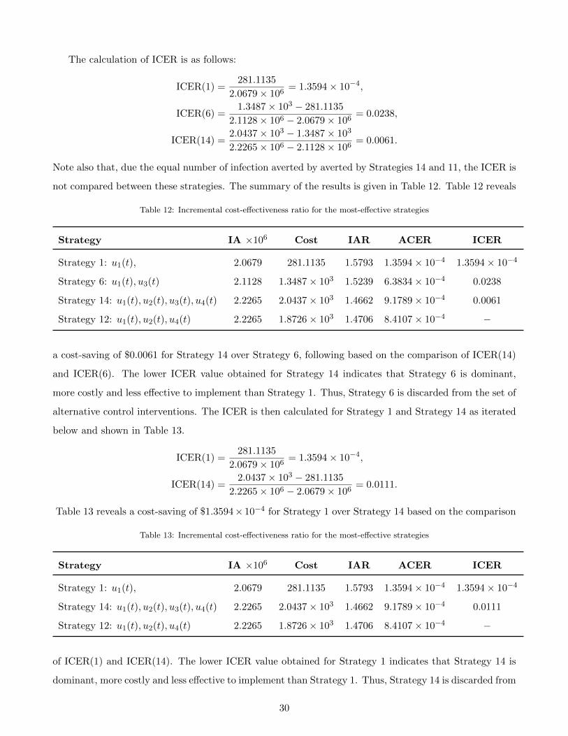
Note also that, due the equal number of infection averted by averted by Strategies 14 and 11, the ICER is
not compared between these strategies. The summary of the results is given in Table 12. Table 12 reveals
Table 12: Incremental cost-effectiveness ratio for the most-effective strategies
Strategy IA ×106 Cost IAR ACER ICER
Strategy 1: u1(t), 2.0679 281.1135 1.5793 1.3594× 10⁻⁴ 1.3594× 10⁻⁴
Strategy 6: u1(t), u3(t) 2.1128 1.3487× 10³ 1.5239 6.3834× 10⁻⁴ 0.0238
Strategy 14: u1(t), u2(t), u3(t), u4(t) 2.2265 2.0437× 10³ 1.4662 9.1789× 10⁻⁴ 0.0061
Strategy 12: u1(t), u2(t), u4(t) 2.2265 1.8726× 10³ 1.4706 8.4107× 10⁻⁴ −
a cost-saving of $0.0061 for Strategy 14 over Strategy 6, following based on the comparison of ICER(14)
and ICER(6). The lower ICER value obtained for Strategy 14 indicates that Strategy 6 is dominant,
more costly and less effective to implement than Strategy 1. Thus, Strategy 6 is discarded from the set of
alternative control interventions. The ICER is then calculated for Strategy 1 and Strategy 14 as iterated
below and shown in Table 13.
ICER(1) =281.1135
2.0679× 106= 1.3594× 10⁻⁴,
ICER(14) =2.0437× 10³ − 281.1135
2.2265× 10⁶ − 2.0679× 106= 0.0111.
Table 13 reveals a cost-saving of $1.3594× 10⁻⁴ for Strategy 1 over Strategy 14 based on the comparison
Table 13: Incremental cost-effectiveness ratio for the most-effective strategies
Strategy IA ×106 Cost IAR ACER ICER
Strategy 1: u1(t), 2.0679 281.1135 1.5793 1.3594× 10⁻⁴ 1.3594× 10⁻⁴
Strategy 14: u1(t), u2(t), u3(t), u4(t) 2.2265 2.0437× 10³ 1.4662 9.1789× 10⁻⁴ 0.0111
Strategy 12: u1(t), u2(t), u4(t) 2.2265 1.8726× 10³ 1.4706 8.4107× 10⁻⁴ −
of ICER(1) and ICER(14). The lower ICER value obtained for Strategy 1 indicates that Strategy 14 is
dominant, more costly and less effective to implement than Strategy 1. Thus, Strategy 14 is discarded from
30

the set of alternative control interventions. The ICER is then recalculated for Strategy 1 and Strategy
12 as iterated below and shown in Table 14.
ICER(1) =281.1135
2.0679× 106= 1.3594× 10⁻⁴,
ICER(12) =1.8726× 10³ − 281.1135
2.2265× 10⁶ − 2.0679× 106= 0.0100.
Table 14 reveals a cost-saving of $1.3594 × 10⁻⁴ for Strategy 1 over Strategy 12 following based on
Table 14: Incremental cost-effectiveness ratio for the most-effective strategies
Strategy IA ×106 Cost IAR ACER ICER
Strategy 1: u1(t), 2.0679 281.1135 1.5793 1.3594× 10⁻⁴ 1.3594× 10⁻⁴
Strategy 12: u1(t), u2(t), u4(t) 2.2265 1.8726× 10³ 1.4706 8.4107× 10⁻⁴ 0.0100
the comparison of ICER(1) and ICER(14). The lower ICER value obtained for Strategy 1 indicates
that Strategy 12 is dominant, more costly and less effective to implement than Strategy 1. Therefore,
comparing the strategies in scenarios A-D, we conclude that, Strategy 1 will be the most cost-saving and
most effective control intervention in the Kingdom of Saudi Arabia. However, in terms of the infection
averted, strategy 6, strategy 11, and strategy 12 and strategy 14 are just as good as strategy 1.
Hence, from these analyses, we see that when one considers the following controls: u1-practising phys-
ical or social distancing protocols; u2-practising personal hygiene by cleaning contaminated surfaces with
alcohol-based detergents; u3-practising proper and safety measures by exposed, asymptomatic infected
and asymptomatic infected individuals; u4-fumigating schools in all levels of education, sports facilities
and commercial areas such as markets and public toilet facilities in Kingdom of Saudi Arabia. u1 (prac-
tising physical or social distancing protocols) has the lowest incremental cost-effectiveness and, therefore,
gives the optimal cost on a large scale than all the other strategies.
5. Concluding remarks
We formulated an optimal control model for the model proposed in [16]. We used four COVID-19
controls in the absence of vaccination thus, practising physical or social distancing protocols; practising
personal hygiene by cleaning contaminated surfaces with alcohol-based detergents; practising proper and
safety measures by exposed, asymptomatic infected and asymptomatic infected individuals; and fumigat-
ing schools in all levels of education, sports facilities and commercial areas such as markets and public
toilet facilities in Kingdom of Saudi Arabia. The implementation of all the control shows that the disease
can be reduced when individuals strictly stick to the proposed controls in this work. The efficacy plots in
31

Figure 5(b) shows that the controls become much more effective after 39 days. We also calculated the in-
fection averted ratio (IAR), average cost-effectiveness ratio (ACER) and the incremental cost-effectiveness
ratio (ICER). We also utilized the cost-minimization analysis when it becomes evident that strategies 11,
12, and 14 had the same number of infection averted.
CRediT authorship contribution statement
All authors contributed equally to the development of this work.
Funding
This work was funded by the National Natural Science Foundation of China under the Grant number:
12022113, Henry Fok Foundation for Young Teachers (171002).
Declaration of Competing Interest
The authors declare that they have no known competing financial interests or personal relationships
that could have appeared to influence the findings reported in this paper.
References
[1] N. Piovella, Analytical solution of seir model describing the free spread of the COVID-19 pandemic,
Chaos, Solitons & Fractals 140 (2020) 110243.
[2] J. Arino, S. Portet, A simple model for COVID-19, Infectious Disease Modelling 5 (2020) 309.
[3] J. Wangping, H. Ke, S. Yang, C. Wenzhe, W. Shengshu, Y. Shanshan, W. Jianwei, K. Fuyin, T. Peng-
gang, L. Jing, et al., Extended sir prediction of the epidemics trend of COVID-19 in italy and
compared with hunan, china, Frontiers in medicine 7 (2020) 169.
[4] Q. Cui, Z. Hu, Y. Li, J. Han, Z. Teng, J. Qian, Dynamic variations of the COVID-19 disease at
different quarantine strategies in wuhan and mainland china, Journal of Infection and Public Health
13 (2020) 849–855.
[5] L. Hu, L.-F. Nie, Dynamic modeling and analysis of COVID-19 in different transmission process and
control strategies, Mathematical Methods in the Applied Sciences (2020) 1–14.
[6] S. Mushayabasa, E. T. Ngarakana-Gwasira, J. Mushanyu, On the role of governmental action and
individual reaction on COVID-19 dynamics in south africa: A mathematical modelling study, Infor-
matics in Medicine Unlocked 20 (2020) 100387.
32

[7] S. M. Garba, J. M.-S. Lubuma, B. Tsanou, Modeling the transmission dynamics of the COVID-19
pandemic in south africa, Mathematical biosciences 328 (2020) 108441.
[8] B. Fatima, G. Zaman, M. A. Alqudah, T. Abdeljawad, Modeling the pandemic trend of 2019 coron-
avirus with optimal control analysis, Results in Physics (2020) 103660.
[9] M. Ali, S. T. H. Shah, M. Imran, A. Khan, The role of asymptomatic class, quarantine and isolation
in the transmission of COVID-19, Journal of Biological Dynamics 14 (1) (2020) 389–408.
[10] L. Lemecha Obsu, S. Feyissa Balcha, Optimal control strategies for the transmission risk of COVID-
19, Journal of biological dynamics 14 (1) (2020) 590–607.
[11] D. Aldila, M. Z. Ndii, B. M. Samiadji, Optimal control on COVID-19 eradication program in indonesia
under the effect of community awareness.
[12] C. T. Deressa, G. F. Duressa, Modeling and optimal control analysis of transmission dynamics of
COVID-19: The case of ethiopia, Alexandria Engineering Journal.
[13] A. Perkins, G. Espana, Optimal control of the COVID-19 pandemic with non-pharmaceutical inter-
ventions, Bulletin of Mathematical Biology 82 (2020) 118.
[14] M. A. A. Oud, A. Ali, H. Alrabaiah, S. Ullah, M. A. Khan, S. Islam, A fractional order mathematical
model for COVID-19 dynamics with quarantine, isolation, and environmental viral load, Advances
in Difference Equations 2021 (1) (2021) 1–19.
[15] J. K. K. Asamoah, M. A. Owusu, Z. Jin, F. Oduro, A. Abidemi, E. O. Gyasi, Global stability and
cost-effectiveness analysis of COVID-19 considering the impact of the environment: using data from
ghana, Chaos, Solitons & Fractals 140 (2020) 110103. doi:https://doi.org/10.1016/j.chaos.
2020.110103.
[16] M. S. Alqarni, M. Alghamdi, T. Muhammad, A. S. Alshomrani, M. A. Khan, Mathematical modeling
for novel coronavirus (COVID-19) and control, Numerical Methods for Partial Differential Equations.
[17] B. Seidu, Optimal Strategies for Control of COVID-19: A Mathematical Perspective, Scientifica
2020.
[18] A. Omame, N. Sene, I. Nometa, C. I. Nwakanma, E. U. Nwafor, N. O. Iheonu, D. Okuonghae,
Analysis of COVID-19 and comorbidity co-infection Model with Optimal Control, medRxiv.
33

[19] J. K. K. Asamoah, Z. Jin, G.-Q. Sun, B. Seidu, E. Yankson, A. Abidemi, F. Oduro, S. E. Moore,
E. Okyere, Sensitivity assessment and optimal economic evaluation of a new COVID-19 compart-
mental epidemic model with control interventions, Chaos, Solitons & Fractals 146 (2021) 110885.
doi:https://doi.org/10.1016/j.chaos.2021.110885.
[20] E. Okyere, S. Olaniyi, E. Bonyah, Analysis of Zika virus dynamics with sexual transmission route
using multiple optimal controls, Scientific African 9 (2020) e00532.
[21] P. Panja, Optimal control analysis of a cholera epidemic model, Biophysical Reviews and Letters
14 (01) (2019) 27–48.
[22] F. Agusto, A. Adekunle, Optimal control of a two-strain tuberculosis-HIV/AIDS co-infection model,
Biosystems 119 (2014) 20–44.
[23] F. Agusto, M. Leite, Optimal control and cost-effective analysis of the 2017 meningitis outbreak in
nigeria, Infectious Disease Modelling 4 (2019) 161–187.
[24] H. W. Berhe, Optimal Control Strategies and Cost-effectiveness Analysis Applied to Real Data of
Cholera Outbreak in Ethiopia’s Oromia Region, Chaos, Solitons & Fractals 138 (2020) 109933.
[25] A. A. Momoh, A. Fugenschuh, Optimal control of intervention strategies and cost effectiveness anal-
ysis for a Zika virus model, Operations Research for Health Care 18 (2018) 99–111.
[26] S. Olaniyi, K. Okosun, S. Adesanya, R. Lebelo, Modelling malaria dynamics with partial immu-
nity and protected travellers: optimal control and cost-effectiveness analysis, Journal of Biological
Dynamics 14 (1) (2020) 90–115.
[27] G. T. Tilahun, O. D. Makinde, D. Malonza, Modelling and optimal control of pneumonia disease
with cost-effective strategies, Journal of Biological Dynamics 11 (sup2) (2017) 400–426.
[28] H. W. Berhe, O. D. Makinde, D. M. Theuri, Co-dynamics of measles and dysentery diarrhea diseases
with optimal control and cost-effectiveness analysis, Applied Mathematics and Computation 347
(2019) 903–921.
[29] H. W. Berhe, O. D. Makinde, D. M. Theuri, Optimal control and cost-effectiveness analysis for
dysentery epidemic model, Applied Mathematics and Information Sciences 12 (2018) 1183–1195.
[30] A. Abidemi, N. A. B. Aziz, Optimal control strategies for dengue fever spread in Johor, Malaysia,
Computer Methods and Programs in Biomedicine (2020) 105585.
34
[31] J. K. K. Asamoah, Z. Jin, G.-Q. Sun, Non-seasonal and seasonal relapse model for Q fever disease
with comprehensive cost-effectiveness analysis, Results in Physics (2021) 103889doi:https://doi.
org/10.1016/j.rinp.2021.103889.
[32] B. Seidu, O. Makinde, C. S. Bornaa, Mathematical analysis of an industrial HIV/AIDS model that
incorporates carefree attitude towards sex, Acta Biotheoretica (2021) 1–20.
[33] M. A. Khan, S. Ullah, S. Kumar, A robust study on 2019-ncov outbreaks through non-singular
derivative, The European Physical Journal Plus 136 (2) (2021) 1–20. doi:https://doi.org/10.
1140/epjp/s13360-021-01159-8.
[34] A. Abidemi, Z. M. Zainuddin, N. A. B. Aziz, Impact of control interventions on COVID-19 population
dynamics in Malaysia: a mathematical study, The European Physical Journal Plus 136 (2) (2021)
1–35.
[35] A.-K. Iddrisu, E. A. Amikiya, D. Otoo, A predictive model for daily cumulative COVID-19 cases in
Ghana, F1000Research 10 (343) (2021) 343.
[36] E. Acheampong, E. Okyere, S. Iddi, J. H. Bonney, J. A. Wattis, R. L. Gomes, Modelling COVID-19
Transmission Dynamics in Ghana, arXiv preprint arXiv:2102.02984.
[37] D. Otoo, E. K. Donkoh, J. A. Kessie, Estimating the Basic Reproductive Number of COVID-19
Cases in Ghana, European Journal of Pure and Applied Mathematics 14 (1) (2021) 135–148.
[38] J. K. K. Asamoah, C. Bornaa, B. Seidu, Z. Jin, Mathematical analysis of the effects of controls on
transmission dynamics of SARS-CoV-2, Alexandria Engineering Journal 59 (6) (2020) 5069–5078.
doi:https://doi.org/10.1016/j.aej.2020.09.033.
[39] M. A. Khan, A. Atangana, E. Alzahrani, et al., The dynamics of COVID-19 with quarantined and
isolation, Advances in Difference Equations 2020 (1) (2020) 1–22. doi:https://doi.org/10.1186/
s13662-020-02882-9.
[40] M. A. Khan, A. Atangana, Modeling the dynamics of novel coronavirus (2019-nCov) with fractional
derivative, Alexandria Engineering Journal 59 (4) (2020) 2379–2389. doi:https://doi.org/10.
1016/j.aej.2020.02.033.
[41] S. E. Moore, H. L. N. Bamen, J. K. K. Asamoah, O. Menoukeu-Pamen, Z. Jin, Global Stability and
Sensitivity Assessment of COVID-19 with Timely and Delayed Diagnosis in Ghana.
35
[42] C. N. Ngonghala, E. Iboi, S. Eikenberry, M. Scotch, C. R. MacIntyre, M. H. Bonds, A. B. Gumel,
Mathematical assessment of the impact of non-pharmaceutical interventions on curtailing the 2019
novel coronavirus, Mathematical biosciences 325 (2020) 108364. doi:https://doi.org/10.1016/
j.mbs.2020.108364.
[43] G.-Q. Sun, S.-F. Wang, M.-T. Li, L. Li, J. Zhang, W. Zhang, Z. Jin, G.-L. Feng, Transmission dynam-
ics of COVID-19 in wuhan, china: effects of lockdown and medical resources, Nonlinear Dynamics
101 (3) (2020) 1981–1993. doi:https://doi.org/10.1007/s11071-020-05770-9.
[44] S. E. Eikenberry, M. Mancuso, E. Iboi, T. Phan, K. Eikenberry, Y. Kuang, E. Kostelich, A. B.
Gumel, To mask or not to mask: Modeling the potential for face mask use by the general public to
curtail the covid-19 pandemic, Infectious Disease Modelling 5 (2020) 293–308. doi:https://doi.
org/10.1016/j.idm.2020.04.001.
[45] L. Lopez, X. Rodo, A modified seir model to predict the covid-19 outbreak in spain and italy:
simulating control scenarios and multi-scale epidemics, Results in Physics 21 (2021) 103746. doi:
https://doi.org/10.1016/j.rinp.2020.103746.
[46] A. Abay, H. W. Berhe, H. A. Atsbaha, Mathematical modelling and analysis of COVID-19 epidemic
and predicting its future situation in ethiopia., Results in Physics (2021) 103853doi:https://doi.
org/10.1016/j.rinp.2021.103853.
[47] B. E. Bassey, J. U. Atsu, Global stability analysis of the role of multi-therapies and non-
pharmaceutical treatment protocols for COVID-19 pandemic, Chaos, Solitons & Fractals 143 (2021)
110574.
[48] F. Agusto, Optimal isolation control strategies and cost-effectiveness analysis of a two-strain avian
influenza model, Biosystems 113 (3) (2013) 155–164.
[49] A. Abidemi, R. Ahmad, N. A. B. Aziz, Global Stability and Optimal Control of Dengue with Two
Coexisting Virus Serotypes, MATEMATIKA: Malaysian Journal of Industrial and Applied Mathe-
matics 35 (4) (2019) 149–170.
[50] J. K. K. Asamoah, F. T. Oduro, E. Bonyah, B. Seidu, Modelling of rabies transmission dynamics
using optimal control analysis, Journal of Applied Mathematics 2017. doi:https://doi.org/10.
1155/2017/2451237.
[51] S. Olaniyi, O. Obabiyi, K. Okosun, A. Oladipo, S. Adewale, Mathematical modelling and optimal
36

cost-effective control of COVID-19 transmission dynamics, The European Physical Journal Plus
135 (11) (2020) 1–20.
[52] J. K. K. Asamoah, Z. Jin, G.-Q. Sun, M. Y. Li, A Deterministic Model for Q Fever Transmission Dy-
namics within Dairy Cattle Herds: Using Sensitivity Analysis and Optimal Controls, Computational
and mathematical methods in medicine 2020. doi:https://doi.org/10.1155/2020/6820608.
[53] J. K. K. Asamoah, F. Nyabadza, Z. Jin, E. Bonyah, M. A. Khan, M. Y. Li, T. Hayat, Backward
bifurcation and sensitivity analysis for bacterial meningitis transmission dynamics with a nonlinear
recovery rate, Chaos, Solitons & Fractals 140 (2020) 110237. doi:https://doi.org/10.1016/j.
chaos.2020.110237.
[54] J. K. K. Asamoah, F. Nyabadza, B. Seidu, M. Chand, H. Dutta, Mathematical modelling of bacterial
meningitis transmission dynamics with control measures, Computational and mathematical methods
in medicine 2018. doi:https://doi.org/10.1155/2018/2657461.
[55] C. R. Rector, C. S, D. J, Principles of Optimization Theory, Narosa Publishing House, New Delhi,
2005.
[56] J. P. Romero-Leiton, J. M. Montoya Aguilar, E. Ibarguen-Mondragon, An optimal control problem
applied to malaria disease in Colombia, Applied Mathematical Sciences 12 (6) (2018) 279–292.
[57] L. Pontryagin, V. Boltyanskii, R. Gamkrelidze, E. Mishchenko, The Mathematical Theory of Optimal
Processes, Wiley, NY, 1962.
[58] F. B. Agusto, I. M. ELmojtaba, Optimal control and cost-effective analysis of malaria/visceral leish-
maniasis co-infection, PLoS One 12 (2) (2017) e0171102.
37