department of electrical and electronic engineering ...hcommin/commintransferreport.pdf ·...

Department of Electrical and Electronic Engineering

Communications and Array Processing Group

Arrayed MIMO Radar

Harry Commin

MPhil/PhD Transfer Report

October 2010

Supervisor: Prof. A. Manikas

Abstract

MIMO radar is an emerging technology that is attracting the attention of both researchers and

practitioners, which employs multiple transmit signals and has the ability to jointly process signals

received at multiple receive antennas. In this report, the various MIMO radar configurations are

defined and discussed. Motivated by its suitability for the direct application of powerful modern

digital array signal processing techniques, the collocated arrays configuration is chosen as the focus

of this report. From this basis, a detailed discussion of performance bounds in array processing

is developed.

The parameter C is introduced as a figure of merit for comparing the performances of practical

direction-finding (DF) algorithms in terms of their superresolution capabilities. C takes values

between 0 and 1, with higher values indicating better resolving capability and C = 1 denotes an

algorithm with the theoretically ideal resolution performance.

Analytical expressions for C can be derived for a number of DF algorithms. In this report,

three such expressions are derived for MUSIC, ‘optimal’Beamspace MUSIC and Minimum Norm.

It is found that optimal beamspace MUSIC yields the smallest resolution separation, which can

approach the ideal when incident signals have equal powers.

Some preliminary work related to an investigation into the role of complex correlation coeffi -

cient is presented. In particular, the 2-emitter CRB is derived for arbitrary correlation, and an

accessible discussion of the spatial smoothing technique is presented. Finally, a variety of impor-

tant topics for significant future research are identified, emphasising the wide-ranging potential

for useful ongoing research contribution in the field of MIMO radar.

2

Contents

Abstract 2

Contents 3

Notation 5

1 Introduction 61.1 Array Configurations in MIMO Radar . . . . . . . . . . . . . . . . . . . . . . . . 71.2 Parameter Estimation . . . . . . . . . . . . . . . . . . . . . . . . . . . . . . . . . 91.3 SIMO Array Signal Model . . . . . . . . . . . . . . . . . . . . . . . . . . . . . . . 101.4 MIMO Radar Signal Model . . . . . . . . . . . . . . . . . . . . . . . . . . . . . . 111.5 The "Virtual Array" Concept in MIMO Radar . . . . . . . . . . . . . . . . . . . . 12

2 Performance Bounds in Array Processing 142.1 Uncertainty Hyperspheres and the Parameter C . . . . . . . . . . . . . . . . . . . 152.2 Theoretical Detection Bounds . . . . . . . . . . . . . . . . . . . . . . . . . . . . . 172.3 Theoretical Resolution Bounds . . . . . . . . . . . . . . . . . . . . . . . . . . . . . 182.4 Theoretical Estimation Error Bounds . . . . . . . . . . . . . . . . . . . . . . . . . 19

2.4.1 Cramer-Rao Bounds . . . . . . . . . . . . . . . . . . . . . . . . . . . . . . 192.4.2 Other Estimation Error Bounds . . . . . . . . . . . . . . . . . . . . . . . . 22

3 Algorithm Comparison using the Figure of Merit C 243.1 Main Results . . . . . . . . . . . . . . . . . . . . . . . . . . . . . . . . . . . . . . 243.2 Discussion . . . . . . . . . . . . . . . . . . . . . . . . . . . . . . . . . . . . . . . . 253.3 Correlated Signals and Spatial Smoothing . . . . . . . . . . . . . . . . . . . . . . 26

4 Conclusions and Future Work 294.1 Conclusions . . . . . . . . . . . . . . . . . . . . . . . . . . . . . . . . . . . . . . . 294.2 Future Work . . . . . . . . . . . . . . . . . . . . . . . . . . . . . . . . . . . . . . . 29

Appendix A Expressing Ideal Resolution Performance in Terms of ξmusic (s) 31

3

CONTENTS 4

Appendix B Lee and Wengrovitz’s Angular Separation Measure 36

Appendix C Ideal Resolution Performance for ULA 38

Appendix D Algorithm-specific Resolution Threshold Expressions 39

Appendix E 2-Source CRB (correlated signals) 41

Appendix F An Accessible Analysis of Spatial Smoothing 44F.1 Relating Source Covariance Matrices . . . . . . . . . . . . . . . . . . . . . . . . . 45F.2 Effective Source Signal Correlation . . . . . . . . . . . . . . . . . . . . . . . . . . 47F.3 Quantifying the Decorrelating Effect . . . . . . . . . . . . . . . . . . . . . . . . . 47F.4 Backward Spatial Smoothing . . . . . . . . . . . . . . . . . . . . . . . . . . . . . . 48

References 50

Notation

a,A Scalara,A Column VectorA,A Matrix(A)ij (i, j)th element of A(·)T Transpose(·)H Conjugate transpose0N (N × 1) vector of zerosIN (N ×N) identity matrixa = vec(A) a is formed by stacking columns of AL [A] Linear subspace spanned by the columns of AL [A]⊥ Complement subspace to L [A]

PA , A(AHA

)−1AH Projection operator onto L [A]

P⊥A , I− PA Projection operator onto L [A]⊥

E {·} Expectation operatorN Number of array antennasL Number of data snapshotsM Number of signal sourcesρ Complex correlation coeffi cientRab Covariance matrix of a and bdiag (a) Matrix whose diagonal elements are given by aexp(a) Element-by-element exponential

5

Chapter 1

Introduction

Radar has received great research interest for many decades [1]. Its basic goal is to provide the

user with information about targets by estimating various parameters of interest (such as target

bearing, range and velocity). In early radar systems, this was achieved by mechanically steering a

directional transmit/receive antenna across the whole space and processing the (electromagnetic)

signals reflected back to the receiver. However, by instead employing an array of multiple antennas

at the transmitter and/or receiver, a number of important breakthroughs in radar theory have

since been made.

Firstly, using the concept of beamforming, an antenna array is able to coherently combine

signals to synthesise a concentrated directional beampattern. This beampattern can be steered

electronically, removing the need for any mechanical steering of the radar platform. Further-

more, with the development of powerful modern digital signal processing techniques, radar theory

has seen dramatic improvement in recent years. In particular, adaptive techniques such as op-

timal beamforming and superresolution direction-finding (DF) have attracted enormous research

interest [2].

The most sophisticated arrayed radar configuration is Multiple Input Multiple Output (MIMO),

whereby the system employs multiple transmit waveforms and has the ability to jointly process

signals received at multiple receive antennas. Due to the general nature of this definition, many

traditional radar configurations can be viewed as (restricted) special cases of the MIMO para-

digm. It is well documented in the literature that harnessing the full potential of MIMO could

offer numerous significant improvements in radar performance, compared to traditional methods.

6

1. Introduction 7

Particularly, since MIMO radars can jointly employ transmit and receive degrees of freedom after

the signal is received, the total number of degrees of freedom available to the system can be greatly

increased. This yields advantages including: improved resolution performance [3] and the ability

to simultaneously detect a higher number of targets (i.e. greater “parameter identifiability”) [4].

"Collocated arrays" is a typical configuration in MIMO radar, whereby transmit and receive

antenna arrays are situated close together (such that the directions to the targets are the same

for both arrays). This configuration will be the main focus of this report. In Section 1.1, all the

various MIMO configurations found in the literature will be reviewed and their relative strengths

and challenges discussed. It will be shown that the collocated configuration is particularly well-

suited to the direct application of adaptive array processing techniques and so the remainder of

this report will focus on such techniques. In Section 1.2, the concept of superresolution direction-

finding (DF) will be introduced. The fundamental bounds on DF performance of an array system

will then be defined and explored. The parameter C is introduced in order to characterise the

impact of practical DF algorithms on resolution performance. C is first derived in general terms,

then specific analytical expressions for C are derived and discussed for the MUSIC, optimal

Beamspace MUSIC and Minimum Norm algorithms for uncorrelated signals. Various topics of

ongoing and future work are discussed in Section 4 and finally the report is concluded in Section

4.1.

1.1 Array Configurations in MIMO Radar

When designing the general physical layout of the antenna arrays in MIMO radar, there are two

main approaches to consider:

1. Widely-separated Antennas [5]

(a) Radar targets are complex bodies composed of many scatterers and so the power of the

signal reflected back to the receiver can vary dramatically even for very small variations

in illumination/observation angle. This can cause severe performance degradation in

radar systems [6]. By distributing (transmit and/or receive) antennas far apart in

space, multiple independent aspects are obtained, significantly reducing the effect of

these fluctuations ("scintillations").

1. Introduction 8

(b) Another useful consequence of the highly diverse signal paths (transmitters to scatterers

to receivers) yielded by this configuration is that the fading properties of each path are

not fully correlated and so a signal decorrelation effect is observed.

(c) Finally, since the targets are illuminated/observed from multiple angles, their velocities

will be different relative to each widely-spaced antenna. This yields a range of different

Doppler frequencies (a “Doppler spread”) which can be exploited to improve moving

target detection (MTD) performance. Specifically, targets with low radial velocity

with respect to one antenna will tend to have a larger radial velocity with respect to

another widely-spaced antenna. Thus, MTD performance for targets which are diffi cult

to distinguish from background clutter is improved.

2. Closely-spaced antennas [7]

(a) Assuming a narrowband signal model, if transmit/receive elements are situated within

the "local region" of a common phase origin, then relative antenna displacements give

rise to consistent, predictable signal phase offsets. This allows array response vectors

to be defined as a function of the array (electrical properties and geometry) and signal

bearings. The array manifold is then defined as the locus of the array response vectors

across the whole parameter space. From this coherent basis, a family of extremely

powerful adaptive array processing techniques can be applied. (These will be discussed

in greater detail in Section 1.2).

In the literature, we find that these two approaches give rise to three possible MIMO radar

configurations:

1. Distributed MIMO Radar: Both transmitters and receivers are widely-separated.

2. Transmit Diversity MIMO Radar: Transmitters are widely-separated and receivers are in a

closely-spaced array.

3. Collocated MIMO Radar: Both transmitters and receivers are in closely-spaced arrays.

Furthermore, these arrays are situated close together (such that target bearings are the

same with respect to both arrays).

1. Introduction 9

Clearly, each of these approaches has their respective strengths and challenges. Transmit

Diversity MIMO Radar has received significant research interest, since it can be considered as

a hybrid approach that seeks to capitalise on the advantages offered by both closely-spaced and

widely-separated antennas [8, 9]. However, this report will be concerned with collocated MIMO

radar since it is the most suited to employing advanced adaptive array processing techniques. A

further major advantage of the collocated arrays configuration is that properties of the transmitted

vector signal are always known to the receiver and, similarly, parameters estimated at the receiver

can be fed back to the transmitter. This provides a basis for the development of novel collaborative

techniques whereby various transmitter characteristics (such as array geometry and waveform

design) can be adaptively optimised depending on parameters estimated at the receiver. Moreover,

the collocated arrays configuration has further practical advantages in that all processing can be

done in situ, without requiring a wireless communication link to a central processor.

1.2 Parameter Estimation

A large part of this report will focus on parameter estimation. In this report, targets are assumed

to be stationary with respect to the radar platform, allowing a strong focus to be placed on the

problem of estimating the directional parameters of targets (direction-finding). Early approaches

to direction-finding with sensor arrays involved simply steering (electronically) a directional beam

around in space and constructing a DF spectrum from the received signal power across the pa-

rameter space. To do this, a complex weight vector (generally designed to be ‘optimal’in some

sense) is used to linearly combine coherent signals into a beam. Since antenna characteristics are

independent of the direction of energy flow, a given weight vector provides the same beampattern

when applied to either transmitting or receiving arrays.

Many optimal beamformers can be found in the literature. The Conventional Beamformer,

due to Bartlett [10], simply uses the manifold vector as the weight vector, which acts to max-

imise expected output power in a data-independent sense. However, significant improvement in

DF performance is offered by beamformers that utilise the received array data (adaptive beam-

formers). A representative early example is Capon’s Maximum Likelihood Method1 [11], which

1For historical reasons, the Capon Beamformer is termed ‘maximum likelihood’, but it generally does notprovide a maximum likelihood estimate in a DF context. It is more correctly referred to as the Minimum VarianceDistortionless Response (MVDR) beamformer.

1. Introduction 10

minimises array output power (variance) subject to the linear constraint that the signal arriving

from the direction of interest is undistorted. While adaptive beamformers have much better reso-

lution performance and interference-rejection capability than data-independent methods, they are

also much more sensitive to modelling errors. Therefore, much research effort has been directed

towards robust adaptive beamforming in recent decades [12].

More recently, a new family of "subspace-based" methods (based on eigenanalysis of the ob-

served signal covariance matrix) have been developed. In general, they take a geometric approach

to the DF problem by seeking to estimate the (orthogonal) signal and noise subspaces (which to-

gether make up the N -dimensional complex space in which the array manifold resides). Manifold

vectors can then be orthogonally projected onto the estimated noise subspace and the norm of

the resulting vector provides a measure of proximity between the two. Repeating this process for

manifold vectors computed across the entire parameter space then provides a DF null spectrum.

(Alternatively, projections onto the signal subspace provide the inverse null spectrum, or "pseudo-

spectrum"). Representative examples are the MUSIC [13] and Minimum Norm [14] algorithms.

As discussed later in this section, the subspace-based approach is capable of yielding extremely

powerful DF performance and so will be a major topic of this report.

In addition to beamformers and subspace-based techniques, several other families of parameter

estimation algorithms can be found in the literature, such as Maximum Likelihood type [15,

Chapter 8] and Parallel Factor Analysis type [16] (of which ESPRIT [17] is a widely-used example).

However, the specific details of the many DF algorithms developed during recent decades are not

central to this report. Such algorithms are reviewed extensively in the literature (see, for example,

[2], [18] and [15, Chapters 7-9]). In this report, a more general theoretical framework will instead

be developed, before later returning to consider specific practical DF algorithms within that

framework.

1.3 SIMO Array Signal Model

In order to aid later discussion regarding direction-finding, a general SIMO (single input, multiple

output) array signal model will be derived first, before expanding to MIMO radar.

ConsiderM narrow-band plane wave signals impinging on an array of N sensors. The (N × 1)

1. Introduction 11

received signal vector at the array output (in the presence of noise) can be modelled as follows:

x(t) = S(θ, φ)m(t) + n(t) (1.1)

where m(t) is the M -vector of the baseband source signals, n(t) is additive noise and S(θ, φ) is

the manifold matrix, having the following structure:

S(θ, φ) = [S(θ1, φ1), S(θ2, φ2), . . . , S(θM , φM)] (1.2)

with parameter vectors θ = [θ1, θ2, . . . , θM ]T and

φ = [φ1, φ2, . . . , φM ]T denoting the directional parameters associated with the M sources (e.g.

azimuth and elevation, where azimuth is measured anti-clockwise from the positive x-axis). The

(N × 1) complex vector S(θ, φ) is the array manifold vector (array response vector):

S(θ, φ) , exp (−jr k(θ, φ)) (1.3)

of the source signal impinging from (θ, φ). In Equation 1.3, the array geometry is represented by

the (N × 3) real matrix:

r , [rx, ry, rz] = [r1, r2, . . . , rN ]T ∈ RN×3 (1.4)

and k(θ, φ) is the wavenumber vector:

k(θ, φ) , 2π

λu(θ, φ) (1.5)

where λ is the signal wavelength and u(θ, φ) is the (3 × 1) real unit vector pointing from (θ, φ)

towards the origin.

1.4 MIMO Radar Signal Model

In its simplest form, a collocated MIMO radar system can be viewed as a SIMO receiver whose

multiple scalar inputs are given by the transmit array’s MISO outputs reflecting from multiple

targets. Denoting transmitter quantities with (·) and assuming targets to be stationary withrespect to the radar platform, the equivalent baseband scalar signal at the kth target can therefore

be expressed as:

zk(t) = SH

(θk, φk)m(t− τ k)

1. Introduction 12

where m(t) is the (N × 1) vector of transmit waveforms and τ k is the time taken for the signal

to propagate from the transmitter to the kth target. The (K × 1) vector signal at the K targets,

z(t) , [z1, z2, . . . , zK ]T , can then be considered to be somewhat analagous to m(t) in the SIMO

array signal model. Thus, assuming collocated arrays, the received signal vector at the array

output is given by:

x(t) =K∑k=1

βkS(θk, φk)SH

(θk, φk)m(t− 2τ k) + n(t) (1.6)

where βk is the complex fading coeffi cient associated with the kth target, which includes path

losses and the target’s radar cross section (RCS). An important point to note is that, unlike in

the general SIMO model, the cross-correlations of the signals at the targets increase as targets

move close together, even if transmit waveforms are orthogonal.

1.5 The "Virtual Array" Concept in MIMO Radar

A problem with the MIMO radar signal model given in Section 1.4 is that the degrees of freedom

are inconventiently distributed amongst the transmitter and receiver. Since the transmit and

receive arrays share a common phase origin, it would be desirable to devise a scheme whereby the

whole system operated coherently. Specifically, it would be constructive to translate all modelled

parameters at the transmitter across to the receiver (or vice versa), so their degrees of freedom

could be combined in a collaborative manner. In the literature, we find that an attempt has been

made to achieve this using the concept of the virtual array [19, 20]. However, we will see that

this approach has crucial flaws that prevent it from being directly applicable to our theoretical

framework at present.

The MIMO radar virtual array concept relies on N equipower, orthogonal transmit waveforms

that can be separated by N matched filters at the outputs of the N receiver antennas. Further-

more, it requires targets to be in the same range bin. In this case the received signal vector at

the output of the array can be written as:

x(t) = Sdiag(β)SHm(t) + n(t) (1.7)

where β , [β1, β2, . . . , βK ]T . The columns of S and S are given by the K source position vectors

1. Introduction 13

associated with the transmit and receive arrays, respectively. Thus, matched filtering yields:

y(t) = E{vec[x(t)mH(t)]}

= E{vec[(Sdiag(β)SHm(t) + n(t)

)mH(t)

]}(1.8)

Since transmit waveforms are orthogonal and equipowered, E{m(t)mH(t)} = IN . Similarly, sincenoise is white, E{n(t)mH(t)} = 0N×N and so:

y(t) = E{vec

[K∑k=1

βkS(θk, φk)SH

(θk, φk)

]}(1.9)

This can be written in the form:

y(t) = E{

K∑k=1

Sv(θk, φk)βk

}(1.10)

where the manifold vector of the virtual array has been defined as:

Sv(θk, φk) , vec[S(θk, φk)S

H(θk, φk)

](1.11)

While the virtual array geometry described by the virtual manifold vector appears promising at

first, the virtual array system as a whole has diffi culties. In particular, it is evident from Equation

1.10 that the virtual SIMO input signals are in fact given by the complex fading coeffi cients,

estimated during the matched filtering process. So, immediately the assumption must be made

that β will exhibit some degree of statistical variance from pulse to pulse (i.e. in slow time),

otherwise no virtual signal power can be observed by the virtual array. However, even if this

assumption is made (i.e. the Swerling II target model is assumed), analysis of the system is

still not straightforward. For example, the finite sampling effect seems diffi cult to define in this

context, since each estimate of β requires multiple snapshots, then each estimate of the covariance

matrix of the virtual array output, Ryy, requires multiple β estimates.Clearly, there are unresolved issues regarding the virtual array. However, since it offers a

potentially huge increase in the number of degrees of freedom, gaining an in-depth understanding

of the virtual array (or developing a more useful alternative) should be considered an important

topic for future research.

Chapter 2

Performance Bounds in Array

Processing

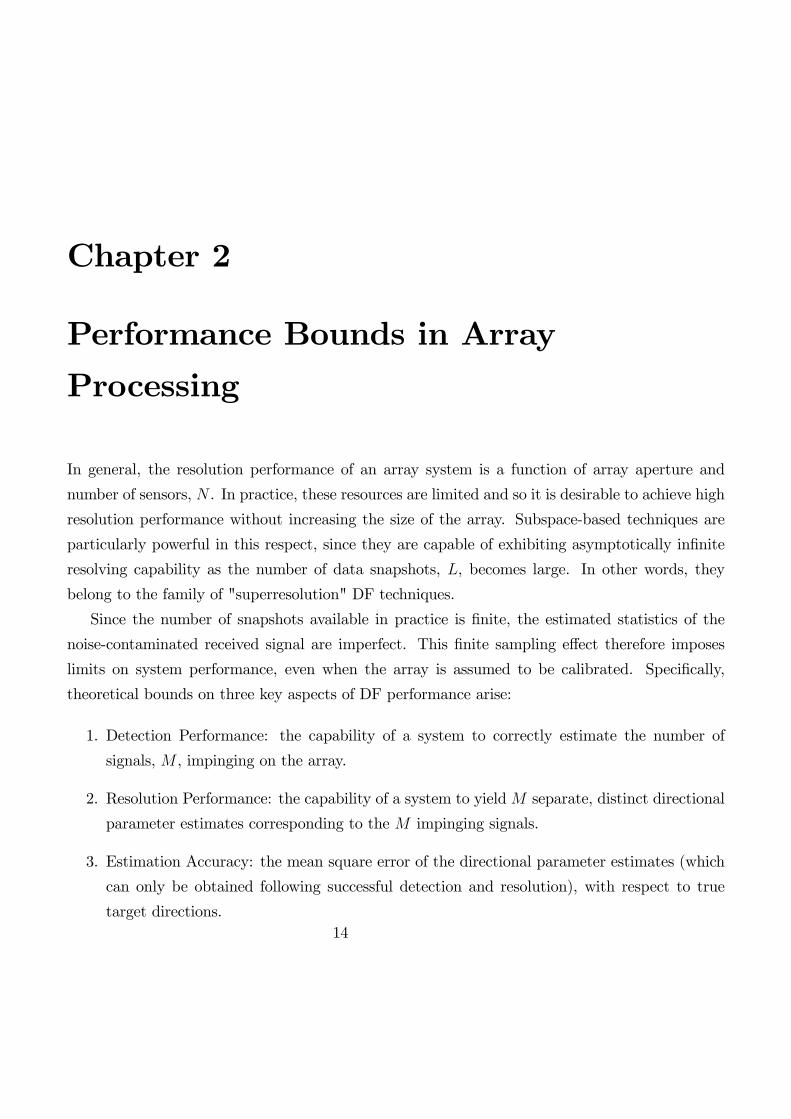
In general, the resolution performance of an array system is a function of array aperture and

number of sensors, N . In practice, these resources are limited and so it is desirable to achieve high

resolution performance without increasing the size of the array. Subspace-based techniques are

particularly powerful in this respect, since they are capable of exhibiting asymptotically infinite

resolving capability as the number of data snapshots, L, becomes large. In other words, they

belong to the family of "superresolution" DF techniques.

Since the number of snapshots available in practice is finite, the estimated statistics of the

noise-contaminated received signal are imperfect. This finite sampling effect therefore imposes

limits on system performance, even when the array is assumed to be calibrated. Specifically,

theoretical bounds on three key aspects of DF performance arise:

1. Detection Performance: the capability of a system to correctly estimate the number of

signals, M , impinging on the array.

2. Resolution Performance: the capability of a system to yieldM separate, distinct directional

parameter estimates corresponding to the M impinging signals.

3. Estimation Accuracy: the mean square error of the directional parameter estimates (which

can only be obtained following successful detection and resolution), with respect to true

target directions.14

2. Performance Bounds in Array Processing 15

In the case of detection and resolution, overall success depends particularly on the two most

closely-spaced sources. Detection and resolution performance can therefore each be characterised

by a different ‘threshold’separation, which must be satisfied in order for detection/resolution to be

achieved with high probability. These thresholds are dependent upon various system parameters

such as: signal-to-noise ratio (SNR), L, N , array geometry, source bearings, relative source powers,

signal correlation and the specific practical DF algorithm employed. In this report, the roles of all

these parameters will be explored in a general sense, except signal correlation; signals are assumed

to be uncorrelated. However, this is considered an extremely important topic for future research

and a preliminary discussion will be developed in Section 3.3.

In order to explore performance bounds in this chapter, the concept of uncertainty hyper-

spheres will first be introduced as a means to characterise the uncertainty in the system due to

the finite sampling effect. While Cramer-Rao bounds are used in the definition of uncertainty

hyperspheres, these will not be discussed in detail until later (in order to preserve the logical order

of: detection, then resolution, then estimation).

2.1 Uncertainty Hyperspheres and the Parameter C

For a given array, the array manifold is defined as the locus of the manifold vectors for all (θ, φ)

across the whole parameter space. In the presence of finite sampling effects, the uncertainty

remaining in the system (corresponding to a given point on the manifold) after L snapshots can

be represented using an N -dimensional hypersphere: It has been proven in [21, Ch. 8, p. 199]

Ndim complex observation space

Figure 2.1: Visualisation of an uncertainty hypersphere in an N -dimensional complex space.


that if the directional parameters, (θ, φ), are expressed as a function of the arc length of the

manifold curve, then the radius, σe, of the uncertainty hypersphere is given by the square root of

the single-source Cramer-Rao Lower Bound expressed in terms of the arc length of the manifold:

σe =1√

2 (SNR× L)(2.1)

This hypersphere therefore represents the smallest achievable uncertainty due to the presence

of noise after L snapshots. In other words, this performance would be achieved by the theoretically

‘ideal’DOA estimation algorithm, whereby any inter-dependency between the various parameters

of the multiple received signals (such as cross-correlation) have been somehow eliminated and no

additional uncertainty has been introduced.

For any non-ideal practical algorithm, this radius will be larger. To model this effect, the

parameter C (where 0 ≥ C > 1) is introduced, which acts to scale the hyperspheres accordingly:

σe =1√

2 (SNR× L)C(2.2)

Clearly, if analytical expressions can be obtained for C for different practical algorithms, then

C can be used as a useful figure-of-merit parameter to compare their performances. This could

provide important insight in a number of ways. Firstly, it will give a clear indication of which

algorithm is the superior for a given scenario (higher value of C denotes superiority). Secondly, if

C is found to be close to 1, then it can immediately be concluded that the algorithm is near-ideal

for that scenario. In other words, if system performance is still unsatisfactory, then there is no

point in considering the use of a more complex algorithm; more favourable scenario parameters

must be sought (for example, by increasing signal powers or the array aperture). Finally, since

C contains all the non-idealities of a given algorithm (and only its non-idealities), the analytical

form of C may provide some insight regarding the cause of these imperfections (and therefore how

to eliminate them).

In Chapter 3, several algorithm-specific expressions for C will be derived and discussed.


2.2 Theoretical Detection Bounds

Detection fails when the estimated number of signals impinging on the array falls below M . For

a subspace-based method, this occurs when the dimensionality of the signal subspace falls below

M . Detection threshold therefore occurs when two uncertainty hyperspheres just overlap (such

that those two sources tend to contribute just one signal eigenvector). This geometrical scenario

is shown in Figure 2.2.

Figure 2.2: Detection threshold occurs when the uncertainty hyperspheres just touch.

It is shown in [21, Ch. 8], that this geometrical model leads to the ‘square root law’ for

detection:

∆pdet−thr =1

s(p1+p22

)(σe1 + σe2) (2.3)

where p represents a directional parameter, such as θ, φ or cone angles [22]. s (p) is the rate of

change of manifold arc length at point p and κ1 is the manifold’s principal curvature (where κ1

also takes into account the inclination angle of the manifold). For a parameterisation in terms of

θ, these properties of the manifold are related to familiar system parameters as follows [23]:

s (θ) = π cos (φ) ‖Rθ‖ (2.4)

κ1 (θ) ≈∥∥∥Rθ

∥∥∥2

(2.5)

κ1 (θ) =

√κ2

1 (θ)−∣∣∣1TN R3

θ

∣∣∣2 (2.6)


where Rθ ,(ry cos (θ)− rx sin (θ)

)and Rθ ,

Rθ‖Rθ‖

.

This allows us to compare ideal detection capability for a variety of array geometries and

scenario parameters, as shown in Figure 2.3.

0 20 40 60 80 100 120 140 160 1805

0

5

10

15

20

Azimuth (degrees)

(SN

RxL

) det,t

hr (d

B)ULANonuniform LinearCircularYshaped

Figure 2.3: Example comparing the ideal detection capabilities of various 25-element uniformly-spaced arrays (dr = λ/2) as a function of azimuth. φ0 = 30◦, P1/P2 = 0.6, ∆θ = 1◦.

2.3 Theoretical Resolution Bounds

Resolution fails when the number of directional parameter estimates falls below M . For a

subspace-based method, this occurs when the number of intersections between the estimated

signal subspace and the array manifold falls below M . The geometry of the resolution threshold

scenario is shown in Figure 2.4, where the signal subspace associated with two sources first fails

to form two distinct intersections with the array manifold.

It is shown in [21, Ch. 8], that this geometrical model leads to the ‘fourth root law’ for

resolution:

∆pres−thr =1

s(p1+p22

)4

√4(

κ21 − 1

N

) (√σe1 +√σe2)

(2.7)

where κ1 is the manifold’s principal curvature and κ1 also takes into account the inclination angle

of the manifold. Again, using the expressions given in [23], a comparison of various ideal resolution


Figure 2.4: Resolution threshold occurs when the worst-case estimated signal subspace justtouches the array manifold.

capabilities for a variety of array geometries and scenario parameters is shown in Figure 2.5.

2.4 Theoretical Estimation Error Bounds

In the literature, a number of approaches can be found that seek to describe lower bounds on

estimation accuracy. These generally involve a discussion of the estimated parameter vector’s

error covariance matrix (since, for unbiased estimators, mean square error and error variance

are equal). Specifically, they seek to set a lower bound on the error covariance matrix of any

estimate, p, of the true parameter vector p , [p1, p2, . . . , pM ]T . In our discussion, a deterministic

signal model [24, 25] is assumed.

2.4.1 Cramer-Rao Bounds

The most popular estimation error bound in array processing is the Cramer-Rao Bound (CRB).

It is a statistical result, based on the inversion of the appropriate Fischer information matrix with

dimension equal to the total number of unknown parameters. Since, in the deterministic model,

the unknown parameters consist of both parameters of interest (DOAs) and nuisance parameters

(e.g. noise variance and complex signal amplitudes), we are actually only interested in a relatively

small submatrix of the inverse Fischer information matrix. An explicit formulation of the relevant


0 20 40 60 80 100 120 140 160 18015

20

25

30

35

40

45

50

55

Azimuth (degrees)

(SN

RxL

) res,

thr (d

B)

ULANonuniform LinearCircularYshaped

Figure 2.5: Example comparing the ideal resolving capabilities of various 25-element uniformly-spaced arrays (dr = λ/2) as a function of azimuth. φ0 = 30◦, P1/P2 = 0.6, ∆θ = 1◦.

submatrix was first introduced in [26] for the single parameter case (e.g. azimuth only), based on

the following assumptions [21]:

A1: N > M and the manifold vectors are independent.

A2: Noise is a zero-mean, temporally white Gaussian process.

A3: Noise is spatially white (from sensor to sensor).

A4: All parameters other than p are known a priori.

The exact Cramer-Rao lower bound on the covariance matrix of the unbiased estimate p of

parameter vector p is given as:

CRB(p) =σ2n

2

(L∑t=1

Re[MH (t)HM (t)

])−1

(2.8)

whereM (t) , diag (m (t)) and H , SHP⊥S S, with P⊥S defined as in the Notation section and S thematrix of manifold vectors differentiated with respect to p. However, a significantly more easily

evaluated (and therefore popular) result is the asymptotic CRB for large L. That is1:

1Note also that a simple extension to the multiple-parameter case (e.g. azimuth, elevation, range) was presentedby Yau and Bresler [27] (also see [28, p. 53])


CRB(p) =σ2n

2L

(Re[H� RTmm

])−1

for suffi ciently large L (2.9)

Since these expressions involve a projection of S (i.e. the sensitivity of the manifold vectors tovariations in p) onto the noise subspace, it can be observed that ultimate estimation accuracy will

therefore increase as the S gradient vectors approach orthogonality to the signal subspace. This

degree of orthogonality is determined by how steeply the array manifold varies for small changes

in p about the direction of interest, pk. Thus, the shape of the array manifold is profoundly and

fundamentally important in determining an array system’s ultimate estimation accuracy. (This

was clearly also the case for detection and resolution).

In practice, we find (see e.g. [21, Fig. 8.4]) that, as angular separation become suffi ciently

large, the CRB in the multiple-emitter scenario approaches the equivalent single-emitter value.

In other words, a wide range of scenarios can be characterised using just two expressions (given

here in terms of geometric properties of the array manifold):

1. The single-emitter CRB:

CRB1[p1] =1

2(SNR× L)s(p1)(2.10)

2. The 2-emitter CRB (for closely-spaced emitters):

CRB2[p1|A] =1

(SNR× L)

2

s(p1)2∆s2(κ21 − 1

N)

(2.11)

where A is the array manifold.While most of this report considers only uncorrelated sources and leaves arbitrary complex

correlation coeffi cient as a topic for future reseach, a new derivation will be presented here. A

partial derivation of the 2-emitter CRB for correlated sources is given in [21, p. 184]. In Appendix

E, this proof is completed by considering the circular approximation to the array manifold. This

yields the final result:

CRB2 [p1] =1

2 (SNR1 × L) s (p1)2

4

(∆s)2 (κ21 (p)− 1

N

) 1(1− Re2[ρ]

P1P2

) (2.12)


It is very interesting to note that this expression comprises three separate contributions:

CRB2 [p1] = CRB1 [p1]×G× S

whereby CRB1 [p1] is the single-source CRB. The real scalar G is a ‘geometry’term, reliant upon

the shape of the array manifold in the neighbourhood of s. Finally, S is a ‘signal’term, dependent

on the statistical properties of the source signals. Clearly, only the real part of the correlation

coeffi cient effects the CRB, but this effect can be reduced by increasing signal powers (which is

consistent with our intuition, when we consider the distribution of data snapshots on the signal

subspace as a function of P1, P2 and ρ).

2.4.2 Other Estimation Error Bounds

Despite its widespread use in the literature, the CRB can be found to be somewhat inadequate

in providing a reliable, tight bound. This is for two main reasons:

1. There exists some threshold (SNR× L), below which the estimation accuracy deviates from

its linear behaviour. The CRB fails to model this large error region (see Figure 2.6).

2. The "estimation error threshold" at which this occurs is not straightforward to predict, so

it is diffi cult to be certain as to exactly what range of (SNR× L) values the CRB is valid

for.

For this reason, estimation error bounds are generally divided into two classes that deal with

each region separately: small-error bounds and large-error bounds (where the CRB is an example

of a small-error bound). Other small-error bounds include the Bhattacharyya inequality (see [29]

and references therein).

The non-linear, high-error region is significantly more computationally complex to model.

Indeed, the original Barankin Lower Bound has therefore seen a number of simplifications, such

as the Chapman and Robbins, Hammersley and Kiefer approaches (and hybrids thereof). These

bounds are discussed in more detail in [15, pp. 1106-1107] and references therein.


CRB

Asymptotic RegionLarge Error RegionNo InformationRegion

SNR x L (dB)

MSE Estimation Error

Threshold

ResolutionThreshold

Figure 2.6: Typical MSE behaviour of a direction finding estimator as a function of (SNR× L),compared with Cramer-Rao bound. (Adapted from: [29]). In a multiple-source scenario, the "NoInformation Region" refers to the sub-resolution-threshold region.

Chapter 3

Algorithm Comparison using the Figure

of Merit C

In Section 2.1, the parameter C was introduced as a figure of merit for comparing superresolution

DF algorithm performance. In this chapter, various algorithm-specific analytical expressions for

C will be derived by studying the resolution capabilities of each algorithm in context to the

theoretically ideal.

3.1 Main Results

By substituting the algorithm-specific resolution threshold expressions given in Appendix D into

the expressions for ideal resolution performance derived in Appendices A and C and using the

relationship derived in Appendix B, the main results of this chapter are now presented. Specifi-

cally, the C parameters for MUSIC, Minimum Norm and optimum Beamspace MUSIC are given

in Equations 3.1-3.4:

24

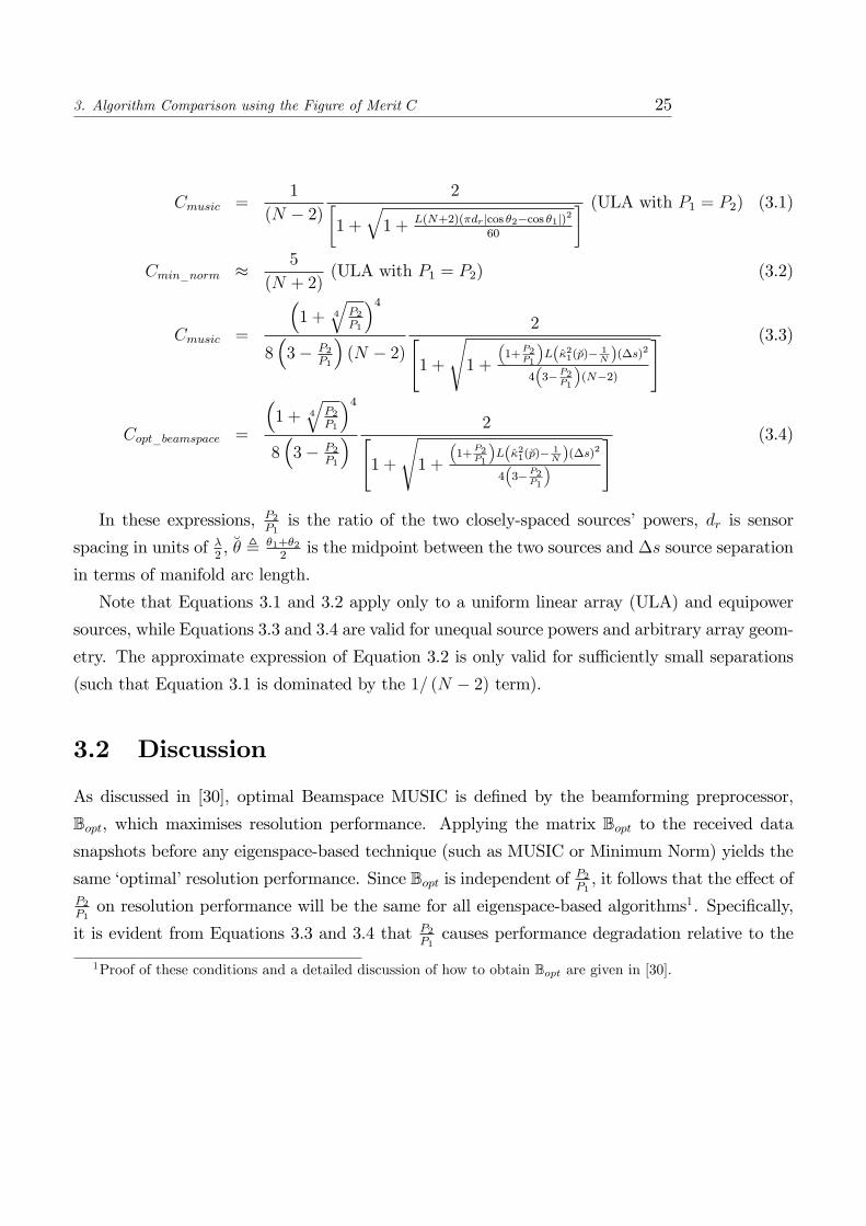
3. Algorithm Comparison using the Figure of Merit C 25

Cmusic =1

(N − 2)

2[1 +

√1 + L(N+2)(πdr|cos θ2−cos θ1|)2

60

] (ULA with P1 = P2) (3.1)

Cmin_norm ≈ 5

(N + 2)(ULA with P1 = P2) (3.2)

Cmusic =

(1 + 4

√P2P1

)4

8(

3− P2P1

)(N − 2)

2[1 +

√1 +

(1+

P2P1

)L(κ21(p)− 1

N )(∆s)2

4(

3−P2P1

)(N−2)

] (3.3)

Copt_beamspace =

(1 + 4

√P2P1

)4

8(

3− P2P1

) 2[1 +

√1 +

(1+

P2P1

)L(κ21(p)− 1

N )(∆s)2

4(

3−P2P1

)] (3.4)

In these expressions, P2P1is the ratio of the two closely-spaced sources’powers, dr is sensor

spacing in units of λ2, θ , θ1+θ2

2is the midpoint between the two sources and ∆s source separation

in terms of manifold arc length.

Note that Equations 3.1 and 3.2 apply only to a uniform linear array (ULA) and equipower

sources, while Equations 3.3 and 3.4 are valid for unequal source powers and arbitrary array geom-

etry. The approximate expression of Equation 3.2 is only valid for suffi ciently small separations

(such that Equation 3.1 is dominated by the 1/ (N − 2) term).

3.2 Discussion

As discussed in [30], optimal Beamspace MUSIC is defined by the beamforming preprocessor,

Bopt, which maximises resolution performance. Applying the matrix Bopt to the received datasnapshots before any eigenspace-based technique (such as MUSIC or Minimum Norm) yields the

same ‘optimal’resolution performance. Since Bopt is independent of P2P1 , it follows that the effect ofP2P1on resolution performance will be the same for all eigenspace-based algorithms1. Specifically,

it is evident from Equations 3.3 and 3.4 that P2P1causes performance degradation relative to the

1Proof of these conditions and a detailed discussion of how to obtain Bopt are given in [30].


equipower case, approximately given by:

Ceigenspace ≈

(1 + 4

√P2P1

)4

8(

3− P2P1

) Ceigenspacegiven

P2P1

=1

(3.5)

which can be approximated by:

Ceigenspace ≈

(4 + 21P2

P1

)25

× Ceigenspacegiven

P2P1

=1

for P2P1& 0.05.

From Equations 3.1-3.3, it can be seen that MUSIC (with arbitrary array geometry) and Min-

imum Norm (ULA geometry) can both exhibit near-ideal performance for 3-element arrays whenP2P1

= 1. However, optimal Beamspace MUSIC can also achieve near-ideal resolution performance

for larger arrays (N > 3), when P2P1

= 1 and the following condition holds:

L(κ2

1(p)− 1N

)(∆s)2

4� 1 (3.6)

Since, (∆s)2 ≈ s(θ)2 |θ2 − θ1|2 (which grows rapidly with increasing N), this condition gener-ally holds for small L, N and |θ2 − θ1|. In Figure 3.1, the C parameters for the three algorithms

are compared for ULAs with increasing numbers of sensors.

In Figure 3.2, the variation of C as a function of azimuth is shown (where the shape of the plot

depends on the array geometry).Optimum Beamspace MUSIC clearly exhibits the best resolution

performance, but its superiority is less outstanding for larger source separations. The same effect

can also be observed for larger numbers of snapshots.

A general trend is that these algorithms perform closer to the ideal when N , L and |θ2 − θ1|are restricted, but there may be considerable scope for improvement by future algorithms that

can better utilise the greater resolving capacity of the system as these quantities increase.

3.3 Correlated Signals and Spatial Smoothing

Our discussion so far has considered only uncorrelated signals. In practice, signals are often

correlated (particularly as radar targets become closely-spaced) and it is well-known that this can


Figure 3.1: Copt_beamspace, Cmin_norm and Cmusic as a function of the number of sensors, N , for aULA. In each case, θ1 = 34◦, θ2 = 35◦, P2

P1= 1 and L = 100.

MUSIC

opt. Beamspace

Figure 3.2: Copt_beamspace and Cmusic for various source separations (for a 25-element uniformX-shaped array) with P2

P1= 1 and L = 100. Since Cmusic is relatively insensitive to changes in

|θ2 − θ1|, the separate traces cannot be distinguished.


severely degrade resolution performance. A popular method of ‘decorrelating’signals is spatial

smoothing [31]. In [32], it is shown that, for two equipowered, fully-correlated (coherent) sources

impinging on a ULA, the resolution performance of the forward-backward spatially-smoothed

MUSIC algorithm is worse by a factor of approximately 4 (Nπdr |cos θ2 − cos θ1|)−2, compared to

the standard, uncorrelated case. However, this result does not provide a great deal of insight into

the effect of arbitrary complex correlation coeffi cient, ρ; like many results found in the literature,

only the fully coherent signals problem is considered (motivated by the multipath propagation

problem in mobile communications, where the primary concern is simply to restore the correct

rank to the resulting covariance matrix).

A major topic for future research related to this project will be to gain a comprehensive

understanding of the impact of ρ on DF performance. As a part of this, it would be constructive

to also fully understand the impact of employing a given decorrelating technique in a correlated

signal environment. In the case of spatial smoothing, we find that there is a trade-off in that a

decorrelation effect can be obtained at the expense of a reduced effective array aperture and with

restrictions imposed on the usable array geometry. However, discussions in the literature on this

topic seem to be particularly inaccessible. Specifically, there seems to be some confusion regarding

the nature of valid subarray geometries and little attention seems to be paid to the analysis of

non-coherent (partially correlated) signals. Therefore, an accessible basic analysis of conventional

and backward spatial smoothing is presented in Appendix F in order to clarify a number of such

points.

Chapter 4

Conclusions and Future Work

4.1 Conclusions

In this report, the various MIMO radar configurations have been defined and compared. Using

the collocated arrays configuration as a basis, a general discussion of parameter estimation in

array processing was then developed. The theoretical performance bounds imposed by the finite

sampling effect on an array system were defined and discussed in detail. The parameter C was

proposed as a figure of merit for comparing superresolution DF algorithms. Representative exam-

ple analytical expressions were derived for the MUSIC, optimal Beamspace MUSIC and Minimum

Norm algorithms (for uncorrelated signals). It was found that, when sources have equal powers,

all these algorithms can offer near-ideal resolution performance for 3-element arrays. However,

only optimum Beamspace MUSIC can achieve this for larger arrays.

Some preliminary work related to the analysis of complex correlation coeffi cient was presented.

In particular, the 2-emitter CRB was derived for arbitrary ρ, and an accessible discussion of the

spatial smoothing technique was presented.

4.2 Future Work

In Section 1.5, a MIMO radar virtual array model was discussed and found to be somewhat flawed.

However, the general concept of reformulating the MIMO signal model into an equivalent SIMO

or MISO system remains a powerful one and should therefore be afforded considerable research

29

4. Conclusions and Future Work 30

effort.

Only a very limited proportion of this report was related to the study of correlated sources.

However, as discussed in Section 3.3, understanding the impact of signal correlation of DF per-

formance is of paramount importance. One possible way to expand our theoretical framework to

allow further insight into this problem could be to slacken the constraint on the definition of the

uncertainty hypersphere’s radius. That is, it should seek to characterise the performance of the

algorithm which is ideal in every sense except with respect to non-zero correlation.

There are several important scenario considerations (in addition to signal correlation) that have

been neglected entirely in this report. Perhaps the most important is non-zero target velocity.

Estimating target velocities by Doppler processing is often a key requirement in radar and so the

system model will need to be changed in order to account for (and ultimately estimate) these

frequency shifts.

Another important consideration is clutter. In radar, signals don’t just reflect back off tar-

gets, but also off clouds, the ground, or any number of objects that we are not interested in.

Distinguishing clutter from targets and rejecting the clutter (whilst preserving as many degrees

of freedom as possible for parameter estimation) is an important challenge.

A further assumption that was made in this report was the narrowband signal assumption.

However, wideband and ultra-wideband MIMO radar are attracting increasing research interest.

This would require a somewhat radical reconsideration of the MIMO system model, since signal

amplitudes and phases will tend to vary across the aperture of the array under the wideband

assumption.

Finally, perhaps the most promising topic for future research will be the development of novel

collaborative techniques, whereby various transmitter characteristics (such as array geometry

and waveform design) can be adaptively optimised depending on parameters estimated at the

receiver. This process of feeding information back from the receiver to the transmitter could be

a particularly powerful utilisation of the collocated MIMO radar configuration.

Appendix A

Expressing Ideal Resolution

Performance in Terms of ξmusic (s)

In this appendix, numerous results are used from [21, Ch. 8]. For notational compatibility,

manifold vectors will therefore be denoted using a (s) here.

The MUSIC [13] null spectrum is given by:

ξmusic (s) = aH (s)P⊥A a (s)

We wish to explore the value in the MUSIC null spectrum associated with the arc length s between

the two sources at s1 and s2. That is:

ξmusic (s) = aH (s)P⊥Aa (s)

= aH (s) (IN − PA) a (s)

= N − aH (s)PAa (s)

The geometric layout is shown in Figures A.1-A.2:

Using these figures, expressions for the required inner product, aH (s)P⊥Aa (s), will now be

developed. In order to do this, a number of related geometric quantities, shown in Figure A.2,

must first be derived:

By first considering the entire (blue) right-angled triangle of Figure A.2, it is clear that:

31

A. Expressing Ideal Resolution Performance in Terms of ξmusic (s) 32

Centre ofCurvature

Origin

Figure A.1: Circular approximation of the array manifold, in the neighbourhood of s.

Centre ofCurvature

Origin

Figure A.2: "Side-on" view, showing a (s) and its orthogonal projection onto the signal subspaceL ([a1, a2]).

cos (γ1) =1

κ1

√N

Using this result, the cosine rule can now be applied to Figure A.3 to determine the angle γ2

between a (s) and PAa (s).

First the length ‖b‖ is evaluated:

‖b‖2 =1

κ21

(1− cos ∆ψ)2 +N − 2

√N

κ1

(1− cos ∆ψ) cos (θ1)

=1

κ21

(χ2 − 2χ

)+N


Figure A.3: Geometric quantities required in the derivation of aH (s)P⊥Aa (s).

where, for notational convenience, χ , (1− cos ∆ψ). Now, applying the cosine rule again:

1

κ21

χ2 =1

κ21

(χ2 − 2χ

)+ 2N − 2

√N

√1

κ21

(χ2 − 2χ) +N cos (γ2)

cos (γ2) =

(N − χ

κ21

)√N√

1κ21

(χ2 − 2χ) +N

The inner product aH (s)PAa (s) can now be evaluated by considering the appropriate right

angled triangle (including the yellow shaded region in Figure A.2). That is, aH (s)PAa (s) =∥∥aH (s)∥∥ ‖PAa (s)‖ cos γ2 = N cos2 γ2 and so:

aH (s)P⊥Aa (s) = aH (s) (IN − PA) a (s)

= N −N cos2 γ2

= N −

(N − χ

κ21

)2(1κ21

(χ2 − 2χ) +N)

By separately evaluating the numerator and the denominator, it is relatively straightforward to

show:

aH (s)P⊥Aa (s) = N −N2 + 2

κ21

[(N − 1

κ21

)(cos ∆ψ − 1)− 1

8‖∆a‖2

]N − ‖∆a‖

2

4

Following a series of straightforward but tedious manipulations, this reduces to:

aH (s)P⊥Aa (s) =

(κ2

1 −1

N

) Nκ41

(cos ∆ψ − 1)2(N − ‖∆a‖

2

4

)


At this stage, the following approximations are used:

Approximation 1 :

cos ∆ψ =

√1− 1

4‖∆a‖2 κ2

1

≈

√(1− 1

8‖∆a‖2 κ2

1

)2

= 1− 1

8‖∆a‖2 κ2

1

Assumption used:1

64‖∆a‖4 κ4

1 �1

4‖∆a‖2 κ2

1

‖∆a‖2 κ21 � 16

Note 1: Since κ1 =∥∥r2∥∥, where ‖r‖ = 1 [21, Table 8.2, p. 186], it follows that κ1 ≤ 1.

Note 2: Since κ1 = κ1 sin ζ [21, Eq. 8.12], κ21 ≤ κ2

1).

Approximation 2 : (N − ‖∆a‖

2

4

)≈ N

Assumption used:

N � ‖∆a‖2

4

Therefore,

aH (s)P⊥Aa (s) ≈(κ2

1 −1

N

) Nκ41

(18‖∆a‖2 κ2

1

)2

N

=

(κ2

1 −1

N

)(1

8‖∆a‖2

)2

=

(κ2

1 − 1N

)(∆s)4

64(A.1)


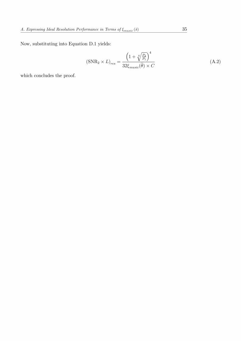
Now, substituting into Equation D.1 yields:

(SNR2 × L)res =

(1 + 4

√P2P1

)4

32ξmusic(θ)× C(A.2)

which concludes the proof.

Appendix B

Lee and Wengrovitz’s Angular

Separation Measure

In this appendix, it is proven that the angular separation measure,∆, given by Lee andWengrovitz

in [30] is, in fact, a scaled small-angle approximation to the change in manifold arc length, ∆s.

The parameter ∆ is given as:

∆2 , k2

N

N∑i=1

[rTi (u(θ2)− u(θ1))

]2=

1

N‖r (k(θ2)− k(θ1))‖2

We know k(θ2)− k(θ1) = π [cosφ(cos θ2 − cos θ1), cosφ(sin θ2 − sin θ1), 0]T and so:

∆2 =π2

Ncos2 φ

N∑i=1

[rxi(cos θ2 − cos θ1) + ryi(sin θ2 − sin θ1)]2

=π2

Ncos2 φ[‖rx‖

2 (cos θ2 − cos θ1)2 +∥∥ry∥∥2

(sin θ2 − sin θ1)2

+ 2rTx ry(cos θ2 − cos θ1)(sin θ2 − sin θ1)

For suffi ciently small |θ2 − θ1|, we have:

cos θ2 − cos θ1 ≈ − sin(θm) |θ2 − θ1|

sin θ2 − sin θ1 ≈ cos(θm) |θ2 − θ1|36

B. Lee and Wengrovitz’s Angular Separation Measure 37

Therefore:

∆2 ≈ π2

Ncos2 φ[‖rx‖

2 (sin(θm) |θ2 − θ1|)2 +∥∥ry∥∥2

(cos(θm) |θ2 − θ1|)2

− 2rTx ry(sin(θm) |θ2 − θ1|)(cos(θm) |θ2 − θ1|)]

=π2

Ncos2 φ |θ2 − θ1|2

[‖rx‖

2 sin(θm)2 +∥∥ry∥∥2

cos(θm)2 − 2rTx ry sin(θm) cos(θm)]

∆ ≈ 1√N|θ2 − θ1| s(θm)

≈ 1√N

∆s for suffi ciently small |θ2 − θ1|

which concludes the proof.

Appendix C

Ideal Resolution Performance for ULA

For a ULA with its phase centre taken to be its centroid (with antenna spacing dr), the sensor

locations are given by:

rx = dr

[−(N − 1)

2,−(N − 1)

2+ 1, . . . ,

(N − 1)

2

]T(C.1)

Using the method of finite differences, it is easily shown that:

‖rx‖ =dr√12

√(N3 −N) (C.2)

Then, using this result, we similarly find:

κ1 =

∥∥∥∥ rx‖rx‖

� rx‖rx‖

∥∥∥∥ =

√3(3N2 − 7)

5(N3 −N)(C.3)

For symmetric linear arrays, κ1 = κ1. Substituting Equations C.2 and C.3 into Equation D.1 and

setting P2P1

= 1 then yields:

(SNR2 × L)res =5760 (πdr |cos θ2 − cos θ1|)−4

N (N2 − 1) (N2 − 4)× C (C.4)

38

Appendix D

Algorithm-specific Resolution Threshold

Expressions

In this Appendix, analytical expressions are derived for the parameter C for MUSIC, optimal

Beamspace MUSIC and Minimum Norm. In order to do this, in each case, an algorithm-specific

resolution threshold expression is first required. Specifically, the results first derived in [33-34]

will be used.

In order to match the conventions of algorithm-specific threshold expressions found in the

literature, it is constructive to express the theoretically ideal resolution performance of Equation

2.7 in terms of (SNR× L):

(SNR2 × L)res =2

∆p4s(p1+p2

2

)4 (κ2

1 − 1N

)C

(1 + 4

√P2

P1

)4

(D.1)

Resolution threshold expressions for each algorithm will now be considered and compared to

Equation D.1.

Following a small modification1, the resolution threshold for the MUSIC algorithm (first de-

1Since the resolution threshold expression given in [33] implies above-ideal performance for suffi ciently smallN , we replace [33, Equation B.1] with a more accurate Taylor expansion. The resulting threshold expression thenagrees with [35].

39

D. Algorithm-specific Resolution Threshold Expressions 40

rived by Kaveh and Barabell in [33]) is shown in Equation D.2:

(SNR× L)(ULA,P1=P2)music =

2880 (πdr |cos θ2 − cos θ1|)−4

N(N2 − 1)(N + 2)

1 +

√1 +

L(N + 2) (πdr |cos θ2 − cos θ1|)2

60

(D.2)

It is valid for two equipower, uncorrelated sources impinging on a uniform linear array (ULA).

In the literature, several attempts to derive the equivalent threshold condition for the Minimum

Norm algorithm can be found. However, these analyses yield different results2. In the absence

of a single, widely-accepted threshold expression, it is simply considered here that Minimum

Norm’s resolution performance is superior to MUSIC’s, according to the following approximate

relationship:

(SNR× L)min_norm ≈(N + 2)

5 (N − 2)(SNR× L)music (D.3)

The above expressions are valid only for equipower sources and ULAs. However, the following

threshold expressions (derived by Lee and Wengrovitz in [30]) are valid for unequal source powers

and arbitrary array geometry:

(SNR2 × L)music =

(3− P2

P1

)(N − 2)

8ξmusic(θ)

1 +

√√√√√1 +16(

1 + P2P1

)Lξmusic(θ)(

3− P2P1

)(N − 2) ∆2

(D.4)

(SNR2 × L)opt_beamspace =

(3− P2

P1

)8ξmusic(θ)

1 +

√√√√√1 +16(

1 + P2P1

)Lξmusic(θ)(

3− P2P1

)∆2

(D.5)

It should be noted that Equation D.1 shows dependency on properties of the differential

geometry of the array manifold. In order to obtain compact expressions for C, Equation D.1

must therefore first be manipulated into a more amenable form. As shown in Appendix C, this

task is simplified significantly by first restricting analysis to the ULA geometry. Furthermore, in

Appendix A, Equation D.1 is expressed in terms of ξmusic(θ) for arbitrary array geometry.

2In [35], an improvement in resolution performance over MUSIC by a factor of approximately 5 (N−1)(N−2)(N−3)(N+2) is

suggested. Meanwhile, a factor of about 5 (N−2)(N+2) can be found in [36]. A similar (but not identical) improvement

of approximately 5 (N−2)(N+2) is also found in [34].

Appendix E

2-Source CRB (correlated signals)

The CRB corresponding to the signal arriving from p1 is given by [21, Eq. 8.36]:

CRB [p1] =1

2 (SNR1 × L)

1

aH1 P⊥A a1

1

1− Re2[ρaH2 P⊥A a1]P1P2(aH1 P⊥A a1)(aH2 P⊥A a2)

(E.1)

Since a1 = u11s (p1) and a2 = u12s (p2), this becomes:

CRB [p1] =1

2 (SNR1 × L)

1

s (p1)2 uH11P⊥Au11

1

1− Re2[ρuH12P⊥A u11]P1P2(uH11P⊥A u11)(uH12P⊥A u12)

(E.2)

The relevant inner products will now be evaluated using the circular approximation to the array

manifold. From [21, Eqs. 8.38-9], we have:

uH11P⊥Au11 =(∆s)2 (κ2

1 (p)− 1N

)4

(E.3)

By symmetry, we also have:

uH12P⊥Au12 =(∆s)2 (κ2

1 (p)− 1N

)4

(E.4)

The quantity uH11P⊥Au12 is less straightforward to evaluate. We commence by following the

method of [21, Eq. 8.96]:

41

E. 2-Source CRB (correlated signals) 42

uH11P⊥Au12 = uH11P⊥a1u12 − uH11P⊥a1a2

(aH2 P⊥a1a2

)−1

aH2 P⊥a1u12

= uH11u12 −(uH11a2a

H2 u12 −

1

NuH11a2a

H2 a1a

H1 u12

)[N

N2 − |aH1 a2|2

]

Now, since aH2 u12 = 0, we have:

uH11P⊥Au12 = uH11u12 +

(uH11a2

) (aH2 a1

) (aH1 u12

)N2 − |aH1 a2|

2 (E.5)

All the remaining inner products follow simply from [21, Eqs. 8.96, 8.100 and 8.105] except for

uH11u12. In this case, using [21, Fig. 8.15], we can see that:

uH11u12 = ‖u11‖ ‖u12‖ cos (2∆ψ)

=√

1− sin2 (2∆ψ)

=√

1− 4 sin2 (∆ψ)[1− sin2 (∆ψ)

]=

√1− ‖∆a‖2 κ2

1 (p)

[1− 1

4‖∆a‖2 κ2

1 (p)

]= ±

(1

2‖∆a‖2 κ2

1 (p)− 1

)Note that for ‖∆a‖ = 0, we have uH11u12 = 1. Thus, taking the negative square root:

uH11u12 = 1− 1

2‖∆a‖2 κ2

1 (p)

Substituting this (and all other relevant inner products) back into Equation E.5, we now proceed

with:

uH11P⊥Au12 = 1− 1

2‖∆a‖2 κ2

1 (p)−‖∆a‖2 (1− 1

4‖∆a‖2 κ2

1 (p)) (N − 1

2‖∆a‖2)

N2 −(N − 1

2‖∆a‖2)2

=‖∆a‖2 (κ2

1 (p)− 1N

)‖∆a‖2N− 4

≈ −(∆s)2 (κ2

1 (p)− 1N

)4

E. 2-Source CRB (correlated signals) 43

(where the assumption 4N � ‖∆a‖2 has been used). Therefore, we have:

uH11P⊥Au11 = uH12P⊥Au12 = −uH11P⊥Au12 (E.6)

and, noting that uH11P⊥Au12 is purely real, Equation E.2 becomes:

CRB [p1] =1

2 (SNR1 × L) s (p1)2

4

(∆s)2 (κ21 (p)− 1

N

) 1(1− Re2[ρ]

P1P2

) (E.7)

Similarly, the bound on arc length is:

CRB [s1] =1

2 (SNR1 × L)

4

(∆s)2 (κ21 (p)− 1

N

) 1(1− Re2[ρ]

P1P2

) (E.8)

Appendix F

An Accessible Analysis of Spatial

Smoothing

The conventional spatial smoothing scheme "decorrelates" signals by employing multiple identical

(possibly overlapping) sensor arrays. (In general, these will be overlapping subarrays of an N -

element array whose full aperture can be utilised when signal correlation is low).

We consider two identical sensor subarrays (with arbitrary 3D geometries given by r1 and r2)

which differ only by a spatial displacement, denoted by the real 3-vector d , [dx, dy, dz]T :

r1 = [r1, r2, . . . , rN ]T (F.1)

r2 = r1 + 1NdT (F.2)

For notational convenience, all quantities associated with the shifted array, r2, will be denoted

using ·. According to the standard narrowband plane-wave signal model, the signals observed atthe outputs of r1 and r2 are given by:

x (t) = Sm (t) + n (t) (F.3)

x (t) = Sm (t) + n (t) (F.4)

respectively. Since the noise is considered to be spatially white, the second order statistics of n (t)

and n (t) are the same. Therefore, the effect of the spatial displacement is contained entirely in

the manifold vectors:44

F. An Accessible Analysis of Spatial Smoothing 45

S (θ, φ) , exp(−jr1k (θ, φ)) (F.5)

S (θ, φ) , exp(−j(r1 + 1Nd

T)k (θ, φ))

= S (θ, φ) exp(−jdTk (θ, φ)) (F.6)

Clearly, shifting the phase origin causes all the components of the manifold vector simply to be

rotated by the same angle in complex space. Crucially, this rotation angle varies as a function of

source bearing, (θ, φ). Specifically, the amount of rotation of the manifold at S (θ, φ) is given by

the inner product of d and k (θ, φ). Note that, due to the plane-wave assumption, an origin shift

perpendicular to source direction k (θ0, φ0) will cause no rotation of the manifold at S (θ0, φ0).

Similarly, for two sources with the same φ, changing dz has no relative rotational effect.

For notational convenience, we denote the complex scalar rotation term as ε and the rotation

angle as α:

ε (θ, φ) , exp(−jdTk (θ, φ))

= exp(−jα) (F.7)

F.1 Relating Source Covariance Matrices

The received signal covariance matrices associated with the two arrays are:

Rxx , E{x (t)xH (t)

}= SRmmSH + σ2

nIN (F.8)

Rxx , E{x (t) xH (t)

}= SRmmSH + σ2

nIN (F.9)

We now note that the matrix of source position vectors associated with the shifted array can be

written as:


S = S

ε (θ1, φ1) 0 0 0

0 ε (θ2, φ2) 0 0

0 0. . . 0

0 0 0 ε (θM , φM)

, SE (F.10)

Therefore,

Rxx = S(ERmmEH

)SH + σ2

nIN

Clearly, we can now explore the relationship between the source covariance matrices associated

with the two subarrays, since we have: Rmm =(ERmmEH

). This relationship is crucial to the

success of spatial smoothing and it arises from the special relationship beteen the subarray sensor

location matrices given in Equations F.1-F.2. In other words, spatial smoothing is valid for any

array geometry that comprises subarrays that differ only by a spatial shift. Note that the MIMO

radar virtual array (under the Swerling II target model) described earlier always carries this

property.

As we would expect, the effect of shifting the phase origin is simply to change the phases of

the correlation coeffi cients relating the various signal pairs (since∣∣εiε∗j ∣∣ = 1):

Rmm ,(ERmmEH

)=

1 ε1ε

∗2 · · · ε1ε

∗M

ε2ε∗1 1 · · · ε2ε

∗M

......

. . ....

εMε∗1 εMε

∗2 · · · 1

� Rmm (F.11)

Thus, the correlation coeffi cients associated with the shifted subarray, ρij, can now be expressed

in terms of ρij:

ρij = εiε∗jρij (F.12)


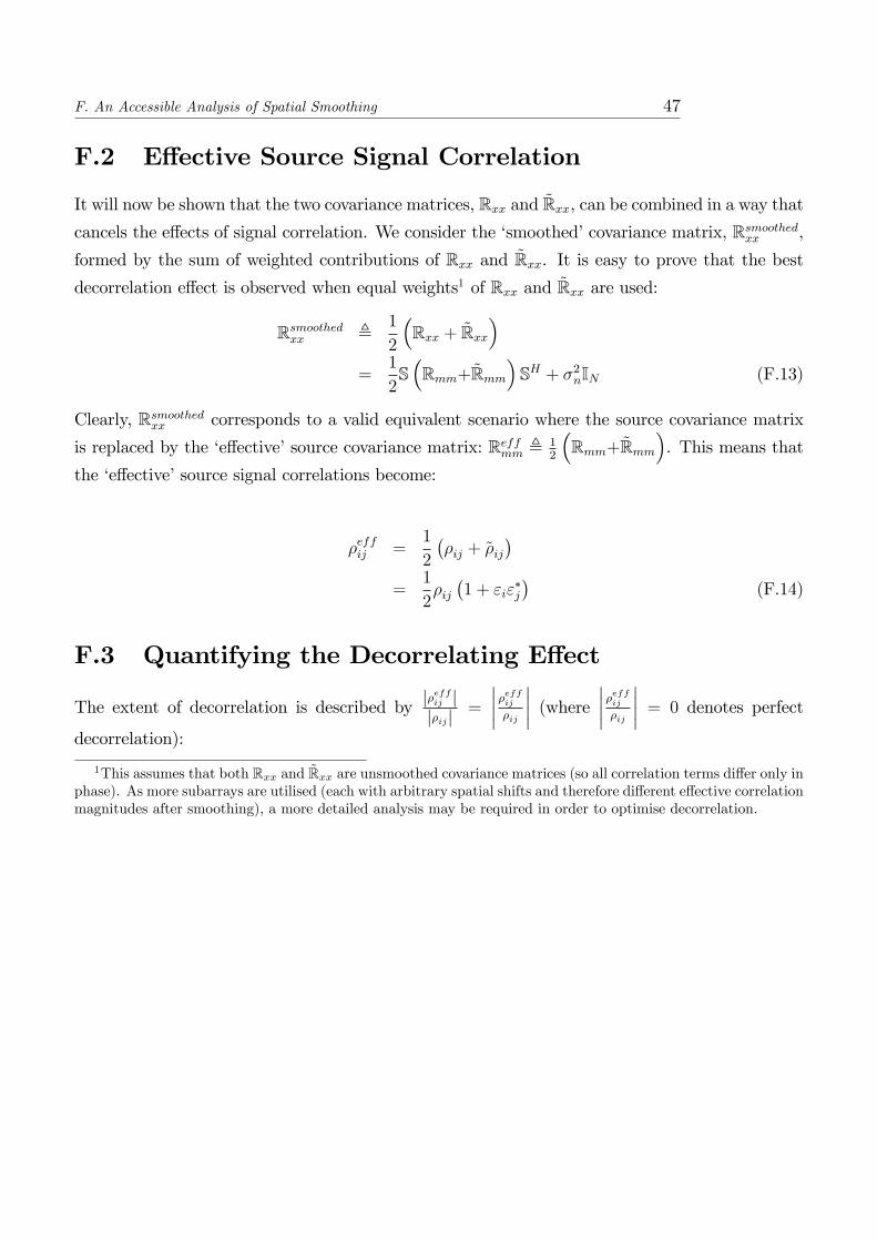
F.2 Effective Source Signal Correlation

It will now be shown that the two covariance matrices, Rxx and Rxx, can be combined in a way thatcancels the effects of signal correlation. We consider the ‘smoothed’covariance matrix, Rsmoothedxx ,

formed by the sum of weighted contributions of Rxx and Rxx. It is easy to prove that the bestdecorrelation effect is observed when equal weights1 of Rxx and Rxx are used:

Rsmoothedxx , 1

2

(Rxx + Rxx

)=

1

2S(Rmm+Rmm

)SH + σ2

nIN (F.13)

Clearly, Rsmoothedxx corresponds to a valid equivalent scenario where the source covariance matrix

is replaced by the ‘effective’source covariance matrix: Reffmm , 12

(Rmm+Rmm

). This means that

the ‘effective’source signal correlations become:

ρeffij =1

2

(ρij + ρij

)=

1

2ρij(1 + εiε

∗j

)(F.14)

F.3 Quantifying the Decorrelating Effect

The extent of decorrelation is described by |ρeffij ||ρij| =

∣∣∣∣ρeffij

ρij

∣∣∣∣ (where ∣∣∣∣ρeffij

ρij

∣∣∣∣ = 0 denotes perfect

decorrelation):

1This assumes that both Rxx and Rxx are unsmoothed covariance matrices (so all correlation terms differ only inphase). As more subarrays are utilised (each with arbitrary spatial shifts and therefore different effective correlationmagnitudes after smoothing), a more detailed analysis may be required in order to optimise decorrelation.


∣∣∣∣∣ρeffij

ρij

∣∣∣∣∣ =

∣∣∣∣12ρij (1 + εiε∗j

)∣∣∣∣=

∣∣∣∣12√(

1 + Re{εiε∗j

})2+ Im

{εiε∗j

}2

∣∣∣∣=

∣∣∣∣12√

(1 + cos (αj − αi))2 + sin2 (αj − αi)∣∣∣∣

=

∣∣∣∣ 1√2

√1 + cos (αj − αi)

∣∣∣∣=

∣∣∣∣cos

(αj − αi

2

)∣∣∣∣ (F.15)

Therefore if |αj − αi| = π, perfect decorrelation is achieved. This is equivalent to spatially shifting

the array in a direction orthogonal to k (θi, φi) until the component parallel to k(θj, φj

)equals

λ2. Clearly, for closely-spaced sources (whose corresponding manifold vectors are almost parallel),

spatial smoothing will tend to be relatively ineffective.

Note that this decorrelation effect is independent of subarray geometry. Since, for a given

overall array geometry, a number of valid subarray geometries can exist, a decision must be made

as to which will offer best overall performance. This will depend jointly on the decorrelation effect

and the subarray geometry’s intrinsic performance bounds.

F.4 Backward Spatial Smoothing

Backward spatial smoothing is valid for a different family of array geometries than forward smooth-

ing. Instead of employing a shifted array, it simply employs the same array in reverse. That is:

r2 = −r1

Therefore, if the sensor locations defined by r1 appear in symmetric pairs about the origin, the

backward array will have identical geometry to the forward array. Thus, their signal/noise sub-

spaces will always be the same and so it is valid to combine their covariance matrices. More


precisely, the backward covariance matrix should be complex conjugated since:

S (θ, φ) , exp(−jr1k (θ, φ)) (F.16)

S (θ, φ) , exp(−jr2k (θ, φ))

= S∗ (θ, φ) (F.17)

and so

Rxx = S∗RmmST + σ2nIN

Conjugating yields:

R∗xx = SR∗mmSH + σ2nIN

Therefore, averaging R∗xx and Rxx is valid and yields the effective source correlation matrix:

Reffmm =1

2(Rmm + R∗mm)

and so effective source correlation ρeffij = 12

(ρij + ρ∗ij

)= Re

{ρij}. In other words, this approach

can eliminate all imaginary components of source correlations (without reducing the aperture of

the array). Note that this backward smoothing effect is independent of all other system parame-

ters.

Clearly, by first shifting a symmetric subarray to the origin, then backward smoothing, a large

variety of forward-backward smoothing operations can be performed for a given array.

References

[1] P. Woodward, Probability and Information Theory with Application to Radar. Artech House,

1953.

[2] H. Krim and M. Viberg, “Two decades of array signal processing research: The parametric

approach,”IEEE Signal Processing Magazine, pp. 67—94, 1996.

[3] D. Bliss and K. Forsythe, “Multiple-input multiple-output (mimo) radar and imaging: De-

grees of freedom and resolution,”Proc. 37th Asilomar Conf. Signals, Syst. Comput., vol. 1,

pp. 54—59, 2003.

[4] J. Li, P. Stoica, L. Xu, and W. Roberts, “On parameter identifiability of mimo radar,”IEEE

Signal Process. Lett., vol. 14, pp. 958—971, 2007.

[5] A. Haimovich, R. Blum, and L. Cimini, “Mimo radar with widely separated antennas,”IEEE

Signal Process. Mag., vol. 25, pp. 116—129, 2008.

[6] E. Fishler, A. Haimovich, R. Blum, D. Chizhik, L. Cimini, and R. Valenzuela, “Mimo radar:

An idea whose time has come,”Proc. IEEE Radar Conf., pp. 71—78, 2004.

[7] J. Li and P. Stoica, “Mimo radar with colocated antennas: Review of some recent work,”

IEEE Signal Process. Mag., vol. 24, pp. 106—114, 2007.

[8] N. Lehmann, E. Fishler, A. Haimovich, R. Blum, D. Chizhik, L. Cimini, and R. Valen-

zuela, “Evaluation of transmit diversity in mimo-radar direction finding,”IEEE Trans. Signal

Processing, vol. 55, pp. 2215—2225, 2007.

[9] M. Jin, G. Liao, and J. Li, “Correlation analysis of target echoes using distributed transmit

array,”Sci China Inf Sci, vol. 53, pp. 1860—1868, 2010.50

REFERENCES 51

[10] M. Bartlett, “A note on the multiplying factors for various chi squared approximations.,”J.

R. Stat. Soc., vol. 16, pp. 296—298, 1954.

[11] J. Capon, “High-resolution frequency-wavenumber spectrum analysis,”Proc. IEEE, vol. 57,

pp. 1408—1418, 1969.

[12] J. Li and P. Stoica, Robust Adaptive Beamforming. Wiley, 2006.

[13] R. O. Schmidt, “Multiple emitter location and signal parameter estimation,” IEEE Trans.

Antennas Propagation, vol. 34, pp. 276—280, 1986.

[14] R. Kumaresan and D. W. Tufts, “Estimating the angles of arrival of multiple plane waves,”

IEEE Trans. Aerosp. Electron. Syst., vol. 19, 1983.

[15] H. L. V. Trees, Optimum Array Processing: Detection, Estimation and Modulation Theory,

Part IV. Wiley, 2002.

[16] N. Sidiropoulos, G. Giannakis, and R. Bro, “Parallel factor analysis in sensor array process-

ing,”IEEE Trans. Signal Processing, vol. 48, pp. 2377—2388, 2000.

[17] R. Roy and T. Kailath, “Esprit - estimation of signal parameters via rotational invariance

technique,”IEEE Trans. on ASSP, vol. 37, pp. 984—995, 1989.

[18] L. Godara, “Limitations and capabilities of directions of arrival estimation techniques using

an array of antennas: A mobile communications perspective,”Proc. IEEE, pp. 327—333, 1996.

[19] I. Bekkerman and J. Tabrikian, “Target detection and localization using mimo radars and

sonars,”IEEE Trans. Signal Processing, vol. 54, pp. 3873—3883, 2006.

[20] C.-Y. Chen, Signal Processing Algorithms for MIMO Radar. PhD thesis, California Institute

of Technology, 2009.

[21] A. Manikas, Differential Geometry in Array Processing. Imperial College Press, 2004.

[22] H. R. Karimi and A. Manikas, “Cone-angle parametrization of the array manifold in df

systems,”J. Franklin Inst. (Eng. Appl. Math.), vol. 335B, pp. 375—394, 1998.

REFERENCES 52

[23] A. Manikas, A. Alexiou, and H. Karimi, “Comparison of the ultimate direction-finding capa-

bilities of a number of planar array geometries,” IEE Proc. Radar, Sonar, Navig., vol. 144,

pp. pp. 321—329, 1997.

[24] P. Stoica and A. Nehorai, “Performance study of conditional and unconditional direction-

of-arrival estimation,” IEEE Trans. Acoust., Speech and Signal Process., vol. 38, no. 10,

pp. 1783—1795, 1990.

[25] A. Matveyev, A. Gershman, and J. Böhme, “On the direction estimation cramer-rao bounds

in the presence of uncorrelated unknown noise,”Circuits, Systems, Signal Processing, vol. 18,

no. 5, pp. 479—487, 1999.

[26] P. Stoica and A. Nehorai, “Music, maximum likelihood and cramer-rao bound,”IEEE Trans.

ASSP, vol. 37, pp. 720—741, 1989.

[27] S. F. Yau and Y. Bresler, “A compact cramer-rao bound expression for parametric estimation

of superimposed signals,”IEEE Trans. Signal Processing, vol. 40, pp. 1226—1229, 1992.

[28] S. Haykin, ed., Advances in Spectrum Analysis and Array Processing, Vol. III. Prentice-Hall,

1994.

[29] A. Alexiou, Bounds in Array Processing. PhD thesis, Imperial College London, 1999.

[30] H. Lee and M. Wengrovitz, “Resolution threshold of beamspace music for two closely spaced

emitters,”IEEE Trans. Acoustics Speech Signal Process., vol. 38, p. 1545U1559, 1990.

[31] T. J. Shan, M. Wax, and T. Kailath, “On spatial smoothing for direction of arrival estimation

of coherent signals,”IEEE Trans. Acoust. Speech Sig. Proc., vol. 33, pp. 806—811, 1985.

[32] U. Pillai and B. Kwon, “Performance analysis of music-type high resolution estimators for

direction finding in correlated and coherent scenes,” IEEE Trans. ASSP, vol. 37, pp. 1176—

1189, 1989.

[33] M. Kaveh and A. Barabell, “The statistical performance of the music and minimum-norm

algorithms in resolving plane waves in noise,” IEEE Trans. Acoust. Speech Signal Process.,

vol. 34, pp. 331—341, 1986.

REFERENCES 53

[34] P. Forster and E. Villier, “Simplified formulas for performance analysis of music and min

norm,”in OCEANS98, Nice, France, 1998.

[35] P. Tichavsky, “Estimating the angles of arrival of multiple plane waves: The statistical

performance of the music and the minimum norm algorithm,”Kybernetika, vol. 24, pp. 196—

206, 1988.

[36] J. Luo and Z. Bao, “The resolution performance of eigenstructure approach,” [Chinese]

Journal of Electronics, vol. 13, 1991.

department of electrical and electronic engineering ...hcommin/commintransferreport.pdf ·...

Documents