ISSN 1753-5816

School of Oriental and African Studies University of London

DEPARTMENT OF ECONOMICS

Working Papers

No.154

INFRASTRUCTURE AS ECONOMIC DENSITY

Sangaralingam Ramesh

December 2007

economics@soas.ac.uk

http://www.soas.ac.uk/academics/departments/economics/research/workingpapers/econ-working-papers.html

1

INFRASTRUCTURE AS ECONOMIC DENSITY Sangaralingam Ramesh ABSTRACT Income disparities are rising in China as a consequence of the economic reforms post 1979 which

virtually gave unchallenged economic growth and prosperity to the coastal regions whose economic

growth increased over the last 30 years at the expense of the interior hinterland. Institutions in China

have seen the answer to restoring a rural-urban income balance by redistributing people from the

interior regions of China to the prosperous coastal regions. This can be seen as a supply side reaction

to the income disparity problem, which will inevitably impose the kinds of social costs, which

concentrations of populations normally bring. This paper offers insights into other methods of

transforming the urban-rural income disparity problem in China, the economic implications of

infrastructure investment, the relevance of Krugmans ‘New Economic Geography’ to the

transformative Economics which China has experienced over the last 30 years; and the close

relationship between how Krugman’s agglomeration economies arise and the development of SEZ’s

and HTDZ’s in China.

2

Introduction

The prosperity of the coastal regions generated through the designation of SEZ’s, creation of open

coastal cities and the creation of the open delta regions has clearly not effectively diffused through to

the central and western regions of China as anticipated by the architects of China’s reforms. Thus, the

income disparity reducing policy of the post 2003 leadership is the mass relocation of people from the

interior hinterland of China to its prosperous coastal regions. However; such a rapid and concentrated

urbanisation program will inevitably lead to the kinds of social costs associated with population

concentrations. Therefore, it would be worthwhile to consider ‘in-situ’ developmental policy

measures. These alternative poverty reduction programs include:

a) Increased investment in agriculture, agriculture is the key externality-generating sector of the

Chinese rural economy. 1

b) Development of non-farm enterprises and investment in town and village enterprises and local

village co-operatives.

c) Increased investment in the so-called knowledge infrastructure in the interior hinterland

(telephones, computers, networks, schools, universities, research institutes and libraries) will

increase knowledge linkages in the Chinese economy and aid the knowledge creation process.

Although, the influx of FDI caused the income divide between the interior of China and the

coastal regions, knowledge creation and transfer has sustained it. This can be clearly seen in

Diagram 1 which shows that in coastal and developed regions such as Guangdong, Zhejiang,

Shanghai, Shenzhen, Jiangsu, Beijing and Shandong the knowledge creation process (as

measured by the number of patents issued) is more pronounced than in central provinces such

as Hunan, Hubei and Henan.Similarly, the knowledge creation process in the central

provinces is more pronounced than the knowledge creation process in the Western provinces

of China such as Tibet, Yunnan and Sichuan.

1 Ravallion, M. "Externalities in Rural Development: Evidence for China." World Bank Policy Research Working Paper (2879).

3

A key feature of the knowledge creation process and the associated agglomeration economies

is that it is location independent, especially with the availability of telecommunications,

computational technology and the Internet. This is in sharp contrast with the agglomeration

economies, which arise from the mutual interdependence of firms at one specific point on the

spatial plain.

d) Another method to reduce rural poverty in the rural setting is to invest massively in hard

infrastructure – building roads, bridges, airports and power stations. This will facilitate the

movement of goods, resources, people and the knowledge creation and transfer process.

0 500 1000 1500 2000 2500 3000 3500

East China

Central China

West China

Diagram 1: Domestic Patents (Invention) Granted By Region

Source: China Statistical Yearbook 2005

Furthermore, investment in hard infrastructure can only serve to motivate entrepreneurial behaviour.

Nevertheless, the focus of this paper will be on factors c) and d), discussed above .The economic

impact of infrastructure, physical and soft, investment in China’s interior provinces will be increased

entrepreneurial activity, increased innovation and economic activity. Chen (1996) points out that

investment in interior infrastructure would raise the incentive for coastal businesses to expand into the

interior and stimulate non-coastal economic growth through the transfer of ideas as well as physical

and human capital. Living in an area with relatively few physical and commercial endowments, in

4

addition to a low population density, may not provide an incentive for farmers living in those areas to

invest in local ventures as externalities may not be generated and they will be no consumption

growth.2 The export oriented economic growth of Southern China illustrates the impact of improved

infrastructure, specifically in the Special Economic Zone’s [SEZ’s ] and High Technology

Development Zone’s[HTDZ’s], on China’s economic growth .The SEZ’s of which the very first was

established in Shenzhen and then the coastal provinces of China at the start of the economic

reforms .On the other hand the HTDZ’s began to be established first in Beijing and then around the

rest of the country with a bigger concentration in the coastal provinces including Jiangsu where four

HTDZ’s out of the fifty-two in the country were established .The precise nature of the linkage

between road infrastructure development and economic growth is unclear, although studies indicate

that the building of roads is a necessary but not sufficient condition for economic growth.3Expansion

of port facilities and improvements in the road network has reduced travel time in the region and this

has enabled the efficient ‘flow of human and capital resources in all directions ‘.4 Panyu, in the Pearl

River Delta is an example of a region where heavy investment in transport infrastructure has led

directly to substantial and prolonged economic growth.5Two infrastructure projects, which contributed

to opening up Panyu to the metropolitan area of Guangzhou, was the building of the Ruoxi Bridge and

the Humen Ferry and Humen Bridge.

Spatial Economics and Regional Growth Strategies

Myrdal (1957), Friedmann (1966), Hirschman (1958) and Krugman (1991) have postulated regional

developmental theories. However, in the literature these theories have not been applied to the

economic development of China to describe its economic evolution since the economic reforms of

1979 or established the role of infrastructure within this body of emerging literature.

2 Ravallion, M. and Jalan. (1999). "China's Lagging Poor Areas." American Economic Review 89(2). 3 Lin, G. (1999),”Transportation and Metropolitan Development in China’s Pearl River Delta: The Experience of Panyu”, Habitat Intl, Vol.23, No.2 PP 249-270. 4 Chan, R. C. K. (1996). “Regional Development of the Pearl River Delta Region Under the Open Policy, Chapter 11 in "China's Regional Economic Development" edited by Chan, R.C.K et al”CUHK. 5 Lin, G. (1999),”Transportation and Metropolitan Development in China’s Pearl River Delta: The Experience of Panyu”, Habitat Intl, Vol.23, No.2 PP 249-270.

5

Myrdal (1957) argues that once a particular region experiences development then this development

will have a momentum of its own drawing in resources, labour and capital from poorer surrounding

areas. Indeed the greater the mobility of labour, capital, resources and trade then the greater will be

what Myrdal (1957) calls the ‘backwash’ effects. These backwash effects relate to periphery regions

losing labour through migration to richer regions and capital due to greater investment returns in

richer regions. These backwash effects are akin to negative externalities i.e. pollution. In the case of

China since economic reforms were started in 1979, there has been a net migration of labour from the

rural sector in the hinterland regions to the booming regions in the coast. Myrdal (1957) also defines

the positive effects of development as spread effects. Friedmann (1966) postulates that the

relationship between central and periphery regions within a country, which are undergoing transition,

is a colonial one. The implication is that there is a net outflow of productive factors of production

such as labour and capital from periphery to centre. Friedmann argues that once this centre-periphery

relationship is established market forces dictate that there will be a divergence in the economic growth

rate of centre and periphery. The centre will grow much faster than the periphery leading to an income

disparity between the former and the latter. Hirschmann (1958) sees disparities in regional income as

the inevitable consequence of economic growth. Indeed government policies designed to address

imbalances in spatial development patterns within a country by promoting growth in poorer regions

may lead to greater disparities within those regions6. This notion that government intervention will

make matters worse is akin to the Classical economic view that markets function best to optimally

allocate resources if they are left to themselves. In the Classical world, the price mechanism is the

method by which the market optimally allocates resources; and thus it supposedly reflects all the

knowledge in the market available to both firms and to consumers.

Krugman (1991), while using the early development theories to develop the

framework of his New Geographical Economics, criticized the early regional development theorists

for their lack of modelling of theory. Krugman (1991) has sought to answer the question ‘Why does

manufacturing end up being concentrated in one part of a country leaving the other parts to play a

6 Barkin, D. (1972). "A Case Study of the Beneficiaries of Regional Development." International Social Developmet Review 4: 84-94.

6

peripheral role?’ In China’s case the answer to this question lies in the fact that government

interference, at odds with the presets of Neo-Classical Economics, by the establishment of SEZ’s and,

at a later stage, HTDZ’s took advantage of the coastal regions comparative advantage in cheap labour,

ease of access of Chinese goods to overseas markets and the efficient use of foreign capital to fuel an

export oriented economic growth strategy. The New Geographical Economics framework was

developed by Krugman in order to explain why economic agglomerations became established in

geographic space. The location of economic agglomerations in the New Geographic Framework is

determined by a mechanism that has microeconomic and not macroeconomic foundations. New

Geographical Economic models are characterised by four characteristics:

a) General economic modelling,

b) Increasing returns to scale or indivisibilities and imperfect competition amongst firms in the

market,

c) Transport costs and,

d) Locational movement of consumers and factors of production towards centres of economic

activity, movement which reinforces agglomeration effects.

Furthermore, there are three types of model in the New Economic Geography:

a) Core-Periphery Models,

b) Regional and Urban system models and,

c) International models.

Core-Periphery models ‘illustrate how the interactions among increasing returns at the level of the

firm, transport costs and factor mobility can cause spatial economic structure to emerge and change

‘.7These types of models have two sectors agriculture and manufacturing and two types of labour the

farmer and the worker respectively. While the latter is mobile between regions, the former is not and

tends to act as a negative force because the farmer is a consumer of agricultural produce and

consumer goods. The negative force is generated via a circular effect of forward and backward

7 Ibid.

7

linkages. According to Fujita & Mori (2005), the factors which induce the core-periphery pattern to

appear include the following:

a) When the transport cost of manufactured goods is low,

b) When consumer expenditure on manufactured goods is large enough and,

c) When types of goods are differentiated.

Following the work of Krugman (1993) and Fujita and Mori (1996) there has not been any significant

research on the spatial distribution of agglomerations and the form of the agglomerations /

dispersions. The former relates to the number, size, location and spatial organisation of

agglomerations and the latter to the degree of urbanisation. The main problem with existing research

is the use of two region models, the use of which in the analysis of spatial relations allows for a lot of

detail to be missed. Fujita and Mori (2005) recognise the latter in the form of qualitative distinctions

between the types and forms of agglomerations and dispersions; and suggest that the problem can be

overcome using the latest computing hardware and software to ‘revisit the possibility of computable

geographical equilibrium models ‘. This development would allow for a more realistic analysis of

spatial topology and allow for conclusions, which reflect reality to be drawn. Thus policy with respect

to what types of infrastructure and other fiscal incentives the government should provide in order to

shape agglomerations and dispersions for the public good can be best formulated.

Cost-minimizing firms will locate their activity at those locations at which sufficient

infrastructure in the form of bridges, roads, airports and ports exist; and at locations at which these

infrastructures can be maintained and built upon. The ability of firms to save costs by choosing to

locate to regions with a degree of infrastructure potential has been shown by Hakimi (1964). Fujita

and Mori (2005) suggest that the location of firms in regions with infrastructure networks and

transport hubs act in such away has to reinforce each other. The infrastructure networks and transport

hubs allow firms to save money in the transport of goods to market and in the transport of

intermediate goods to firm’s production sites. Moreover, the location of a firm is important because it

allows the ease of mobility of senior personnel; and will ensure that non-production costs associated

with differentiating a firm’s product can also be minimised. Cost minimizing firms through

agglomeration economies will reinforce the infrastructural / transport hub by increasing the demand

8

for transport, its efficiency and its provision .The more frequent the services, say at a port, then more

exporters will be attracted and more services would be provided and so on. It has been suggested in

the literature that this self-supporting mechanism leads to the ‘endogenous formation of trunk links

and transport hubs ‘; and the circular causation of demand /supply of infrastructure can be called the

economies of transport density.8

The transport network was not factored into the NEG framework until Takahashi (2005)

.He again used a two-region set-up to endogenise the transport network and consequently he provided

a microfoundation for the economies of transport density. However, Fujita & Mori (2005) criticize

Takahashi because the latter’s two region model does not allow for transport hub formation, the

consequence of which is that there is no explanation for the interdependence of consumer and firm

agglomerations and transport network structure. Thus, Fujita & Mori (2005) feel that there is room for

more research into spatial distribution of economic agglomerations and placing transport activities

firmly within the confines of a model can extend the structure of the transport network; and the New

Economic Geography.

One major criticism of the New Economic Geographic framework is that it only accounts for

the creation of agglomeration effects, which arise due to externalities caused by physical linkages

amongst consumers and firms in geographic space. Consequently and implicitly, it excludes

agglomeration effects, which are caused by knowledge linkages generated by knowledge externalities.

Fujita & Mori (2005) suggest that the exclusion of agglomeration forces caused by knowledge

creation from the original framework of the New Economic Geography was because it had to operate

within the toolbox of general equilibrium economics, with its assumption of perfect knowledge.

Therefore, the market optimally allocates scarce resources through the price mechanism, which

reflects all known knowledge; and thus there is no allowance for the creation of knowledge.

Empirical Infrastructure

A number of researchers have conducted empirical work to establish a link between infrastructure and

economic development. Bao et al (2002) surmises that ‘the spatial and topographic advantages of the

8 Fujita, M. and Mori, T (2005). "Frontiers of the New Economic Geography." IDE Discussion Paper (27).

9

coastal provinces are realised ‘. Indeed the economic model they devised and the subsequent results of

the regression analysis carried out using that model, indicate that:

a) The proportion of the population who are 100km from the coastline can explain 33% of the

variation in provincial GDP.

b) The coastline length can explain 68% of the variation in provincial GDP.

Thus, the greater the proportion of a countries population within 100km of the coast and the greater

the coastline of the country, the greater will be its GDP. Similarly, the smaller the proportion of a

countries population located within 100km of the coast and the smaller the coastline of a country, the

smaller will be its GDP.So it is possible that a country that is landlocked will have a low GDP. One

can compare the Chinese hinterland with a landlocked country; because the greater the distance of a

province from the sea then the greater degree to which it is landlocked. Limao and Venables (2001)

using gravity models study ‘the determinants of transport costs and show how they depend on

countries geography and on its level of infrastructure.’ They focus on the distance between two

countries regardless of the fact that they may be landlocked, share a common border or are islands.

The measure of infrastructure they use relates to the quality of transport and communications

infrastructure. They show that ‘improvements in the infrastructure of landlocked countries and their

transit countries can dramatically increase trade flows’. Demurger (2001) has;

1) Estimated a growth equation using a standard Barro-type framework. Furthermore ,using this

framework Demurger(2001) has showed that a set of variables reflecting differences in steady

state equilibrium could be added to a Solow type equation and conditional convergence tested for.

2) Found that across the provinces of China, location and infrastructural endowments played a

significant role on regional economic growth. More specifically the economic reforms have

allowed ‘urbanised provinces to grow at a higher rate than rural provinces; and poorer provinces

would gain more from infrastructure investment than provinces, which are already well endowed

in infrastructure.

3) Provided empirical evidence as to why economic growth has been so different across provinces

and on the specific relationship between provincial infrastructure endowments and provincial

economic growth.

10

4) Found that road network density decreases as one moves from the coastal provinces to the

western provinces. In addition, non-coastal provinces with a good endowment of transport

facilities are located near coastal provinces. Those non-coastal provinces i.e. Shanxi with a good

endowment of transport facilities owe it to the location of a strategic industry within its borders or

the location of the province i.e. Hubei and Anhui to a major waterway like the Yangtze.

However, energy resource and relatively remote provinces such as Ningxia, Inner Mongolia or

Xinjiang have a very low transport density network. There is also a correlation between the level

of telecommunications endowment in a province and the level of transport network density in that

province. Provinces where the number of telephones per capita is higher than average are also

provinces where the transport network density is over 350km per 1000 2km .

5) Argued that total factor productivity growth is a function of infrastructure endowment on the

assumption that developed infrastructure facilities makes it easier for entrepreneurs to use new

technology, generating technical progress and thus economic growth .In a country like China

where vast distances separate the sites of light manufacturing industry from sites of energy and

raw material sources, the role of telecommunications and transport in allowing local

entrepreneurs to use imported technology is especially significant .Without the basic

infrastructure in place to link producers of goods and services to the suppliers of raw materials

and energy ,inefficiencies and lack of competitiveness may impede economic development 9.

Demurger (2001) concludes her paper suggesting that ‘geographical location, transport infrastructure

and telecommunication facilities do account for a significant part of the observed variation in the

growth performance of provinces’ in China.

The link between infrastructure and Total Factor Productivity or TFP has been

established by a number of studies:

9 Demurger, S. (2001). "Infrastructure Development and Economic Growth: An Explanation for Regional Disparities in China?" Journal of Comparative Economics 29: 95-117.

11

a) Fleischer and Chen (1997) used the transport route length in 1986 as an explanatory variable for

TFP level and growth in Chinese provinces from 1978 to 1993. But they did not find any

significant contribution to the TFP level by transport infrastructure.

b) Mody and Wang (1997) however, using panel data, find that the road network length and

telecommunications facilities were ‘engines of growth ‘in the period examined.

Roller and Waverman (2001) have studied the effects of telecoms infrastructure on economic

development, using data from 21 OECD member countries over a 20-year period, and its impact on

economic development. Their findings indicate that there is a casual link between the two, especially

when a ‘critical mass of telecommunications infrastructure is present.’ Furthermore, they find that this

critical mass leads to increasing returns as the level of telecoms in the economy approaches what can

be defined as a universal level of service. In addition as the level of telecoms infrastructure in the

economy increases, higher economic growth effects are more likely to occur in OECD countries than

less well-developed OECD countries.

Spiros et al (2000) consider infrastructure has a cost reducing technology and has such it

promotes specialisation, leading to the division of labour in the production of goods, and long run

economic growth .The latter is non-monotonic and this reflects the resource costs incurred by

infrastructure investment. They find that’ the degree of specialisation is positively correlated with

core infrastructure’. At the end of their paper Spiros et al (2000) suggest that ‘modelling soft

infrastructure is likely to yield further important insights into the process of economic growth ‘. The

provision of infrastructure leads to the increased mobility of labour and therefore an increased

division of labour, which leads to specialisation in the production of final goods. However, now it has

been established that infrastructure acting as a production technology will lead to the reduction in the

fixed costs of producing intermediate goods and therefore facilitates specialisation in the production

of final goods .The fixed costs relate to the cost of transporting manufactured goods to market and

transporting factors of production to the site of production.

Bougheas et al (1999) explore the relationship between the stock of infrastructure and the volume

of trade. They postulate that ‘infrastructure influences transport costs’ and thereby influence the

volume of trade. The model they use, not surprisingly, predicts a positive relationship between the

12

stock of infrastructure and the volume of trade. Furthermore, they predict that additional increases in

the level of infrastructure are not always welfare increasing but may lead to loss of final output.

Holtz-Eakin & Lovely (1996) have researched the productivity of public infrastructure. Their research

suggests that ‘infrastructure lowers costs in a manufacturing sector characterized by firm level returns

to scale and industry level external returns to variety ‘. Furthermore, infrastructure will alter factor

prices and the distribution of factors of production across sectors. They also find that the provision of

infrastructure by public means increases the number of manufacturing establishments and therefore

manufacturing output.

Amiti and Javorcik (2005) have done some work on ‘Trade Costs and Location of Foreign Firms

in China ‘. They constructed measures of supplier access and market access based on inter-provincial

distances, values of output classified by industry/province and national input/output tables. Trade

costs were proxied by provincial level infrastructure development and how open the province was to

international trade. Electricity charges and the cost of labour proxied production costs. Their study

indicates that supplier access, market access, trade costs and factor costs are the most important

factors when foreign firms consider opening up operations in China. Furthermore, supplier and market

access in the province in which foreign firms open up operations is more important than supplier and

market access to other provinces in China. In addition:

a) Supplier and market access are the two most important determinants of FDI,

b) The existing pool of customers and suppliers in the market are more important to potential

investors of FDI than those in other parts of China,

c) It can also be deduced from their findings that provinces with the greatest provision of

transport infrastructure attract the biggest share of foreign entry. To this end they model

‘transport costs as a function of distance; and the availability of infrastructure is mimicked by

the inclusion of the length of railroads and sea and river berths.

While others have done research on FDI determinants of a firm’s locational investment decision,

little work has been done on the spatial aspects of a firms locational investment decision .The

literature is extended in three ways by the analysis of Amita and Javorcik (2005):

13

a) The spatial aspects of market and supplier access which determine firm entry into the Chinese

market are considered,

b) Inter-industry linkages are taken into account in considering measures of supplier access and

market access and,

c) Aspects of the new economic geography are used to explore the importance of market size

and production costs in attracting foreign firms into the market.

In contrasting the importance of supplier and market access as opposed to the importance of

production costs in attracting foreign firms to set up operations in a province, Amiti and Javorcik

(2005) are able to indicate the best policies ‘in attracting FDI to disadvantaged regions.’ The study by

Amiti and Javorcik (2005) also indicates that Chinese provinces suffer from the ‘infant industry

‘syndrome, that is provincial governments protect local industries from competition from industries in

other regions. Thus, the central government must act to enforce national infrastructural policy at the

local level.10 Concluding their paper, Amiti and Javorcik (2005) suggest that ‘dismantling inter-

provincial barriers, and improving transport infrastructure will increase market and supplier access for

both Chinese and foreign producers, attracting entry of new firms ‘.

Luo (2004) suggests that if infrastructure investments were focused in the development of

‘central transportation hubs’ in the provinces of Hubei, Henan and Hunan then this strategy would

maximise development across all provinces, rather than in any specific ones. Such a strategy would

therefore favour balanced regional growth. The development of central transportation hubs also

lowers the costs of transportation of manufactured goods and factors of production from the western

provinces of China to the coastal provinces. The continuing underdevelopment of the western regions

of China only hinders the integration of the fragmented markets of China; and promotes poor

economic growth of the western provinces and social unrest within them.11

10 Speece, M. W. and Kawahara, Y (1995). "Transportation in China in the 1990's." International Journal of Physical Distribution and Logistics Management 25(8). 11 Luo, X. (2004). "The Role of Infrastructure Investment Location in China's Western Development." World Bank Working Paper 3345(June 2004).

14

After the launch of the market reforms in 1979 and the subsequent divorce of economic

management and state administration at provincial level, agricultural growth in China experienced

rapid growth, defining the impact of rural infrastructure in three ways12:

a) Increased agricultural productivity,

b) Intra-provincial migration from rural areas to urban regions, factor mobility, and,

c) Increased non-farm employment in rural areas.

By carrying out a regression analysis, using recently available data on rural infrastructure Fan and

Zhang (2004) draw two conclusions:

a) Infrastructure and education play a key role in the difference in rural non-farm productivity

than rural agricultural productivity. They point out that, as rural non-farm production is a

significant determinant of rural income then investing in rural infrastructure will lead to an

increase in rural wealth.

b) In the western regions of China agricultural production is low because of a lack of rural

infrastructure, low levels of education amongst the rural population and low levels of science

and technology. The lack of local revenue is also a hindrance to investment in rural

infrastructure in the western regions. This combined with the lack of diffusion of prosperity

from the coastal regions of China to the western regions as led to the government directing

public investment, a core part of the 10th 2001-2005 five year plan, into rural infrastructure in

the western regions, under the umbrella of the ‘Western Development Programme’.13

In developing the New Economic Geography framework, Krugman sought to make use of the

unmodelled theories of the early regional developmental theorists and in doing so modelled the New

Economic Geography using what is essentially a core-periphery framework. However, in the

economic development of China the New Economic Geography is abstract because the framework

does not address the three fundamental forces and stages, which have characterised China’s economic

growth:

12 Fan, S and Zhang, X (2004). "Infrastructure and Regional Economic Development in China." China Economic Review 15: 203-214.

13 Brun, J. F., Combes, J.L and Renard, M.F (2002). "Are there spillover effects between coastal and noncoastal regions of China?" China Economic Review 13: 161-169.

15

a) Manufacturing and the SEZ’s and HTDZ’s, agriculture playing an insignificant role,

b) Knowledge transfer and,

c) Knowledge creation.

There is thus a need to revisit the New Economic Geography and adapt it for the China context.

Furthermore, none of the empirical studies discussed above have specifically looked at the link

between infrastructure and knowledge creation and how this fits in the New Economic Geography.

Krugman’s New Economic Geography Revisited

As previously discussed Krugman (1991) has sought to answer the question ‘Why does manufacturing

end up being concentrated in one part of a country leaving the other parts to play a peripheral role?’ In

the China case the answer to this question arises from the fact that due to government interference

SEZ’s were established due to the inception of economic reforms in 1978, first in Shenzhen and then

in other coastal regions of China, to be followed by HTDZ’s in order to realise China’s comparative

advantage in cheap labour, ease of access of Chinese goods to overseas markets and the efficient use

of foreign capital. The economic development of China since 1978 has led to the manufacture of light

goods and high technology goods being concentrated in the coastal provinces with agriculture

remaining the way of life for a significant majority of China’s population in its interior hinterland.

Special Economic Zones (SEZ’s) have allowed for the export led manufacture of light goods and this

was followed by the High Technology Development Zones (HTDZ’s) which facilitated the export of

high technology goods in the coastal provinces has given these provinces an advantage in terms of

economic and social prosperity, contributing to the increase in income disparity between the coastal

provinces and China’s interior hinterland. The main essence of both SEZ’s and HTDZ’s is that they

represent points in space where firms and physical infrastructure are concentrated , where knowledge

transfer occurs between Chinese companies and foreign MNC’s through joint ventures ;and the

employment of Chinese nationals in foreign MNC R&D centres .The Chinese economy has moved

from the stages of the manufacture of light goods , the production of technological goods through

16

knowledge transfer and is now on a trajectory for economic growth through endogenous knowledge

creation specifically due to the governments policy of ‘endogenous innovation and harmony’ .

A critical appraisal of the various aspects of the New Economic Geography reveals that in his model,

Krugman (1991) has:

a) Only considered the agricultural and manufacturing sector,

b) Not considered the role of knowledge creation,

c) Assumed that the core-periphery pattern forms due to pecuniary externalities, that

manufacturing is concentrated in order to minimise transport costs and has therefore

objectively excluded the role of infrastructure in economic development.

d) Assumed that the peasant population is immobile between regions. This is quite unrealistic

because people move to places where jobs are being created. This is the same the world over as well

as in China.

In the China context Krugman’s New Economic Geography is abstract because:

1) Its economic growth has been driven by the manufacturing sector with agriculture playing an

insignificant role.

2) China’s transition to an industrialised economy has necessitated the movement of peasants

from the rural hinterland (periphery) to the coastal regions (core).

3) Due to the role of FDI China’s transition to a market economy has been characterised by

knowledge transfer, which is itself transitioning to a knowledge creation economy.

In the light of these differences between theory and practice, perhaps a reappraisal of the framework

of the New Economic Geography is in order.

Extending Krugman’s New Economic Geography

Krugman’s theory is based on the neo-classical production function where the only deviations are

increasing returns and imperfect competition. Nevertheless, the increasing returns which arise from

the fixation of agents and factors of production in one point on the spatial plain excludes the

increasing returns which may arise due to knowledge creation. Innovation is assumed to be exogenous

to the neoclassical production function; and is the mechanism by which firms and the aggregate

economy’s Production Possibility Frontier are assumed to grow. However, due to the assumption of

17

perfect knowledge in Neoclassical Economics the agglomeration economies, which arise from

knowledge creation, are not accounted for by the New Geographical Economics.

Towards an Alternative Model

In the light of the above discussion ,both theoretical and empirical it is clear that little work as been

realised on Infrastructure ,Knowledge Creation ,Knowledge Transfer and economic growth in China

within the framework of the New Economic Geography [NEG] . Thus, it is now sought to

quantitatively analyse the role of infrastructure and knowledge creation, which is not accounted for by

the NEG, in China’s economic growth; and extend the work of previous authors. In this context it is

best to look at the neoclassical production function and establish how it can be modified to relate to

recent economic history .The neoclassical production function can be represented by the equation:

),( LKFY =

Where =Y output, =K capital and =L labour.

This model represented by this equation is clearly outdated and is in need of extension .One possible

solution, which while allowing for constant returns to scale can also factor in increasing returns due to

the knowledge creation process, is as follows:

!!"#"+= ))L(A(K))L(A(KY

S

tIFPst

1US

tMFPhtt ……………………………………………… (1)

Taking logs on both sides equation (1) is transformed to:

S

tIFPst

US

tMFPhtt L)A(Log)K(Log.)L(Log)1()A(Log)1()K(Log)Y(Log !+!+!+"#+"#+"=!" … (2)

In equation 1 the variables are as follows:

=!

htK Capital with regards to hard infrastructure.

=MFPA Technological Innovation – Manufacturing Factor Productivity.

=US

tL Unskilled Labour in the Primary Sector

=!

stK Capital with regards to soft infrastructure

=IFP

A Technological Innovation – Intellectual Factor Productivity.

=S

tL Skilled Labour in the Tertiary Sector

18

Where 10 !"< and 10 >! " ; and IFPMFP

AATFP +=

The model described by equation (1) describes a production function, which is composed of two

parts. The first describes the inputs into manufacturing and the second part of the equation describes

the inputs into the knowledge creation process. In manufacturing fixed capital investment and

unskilled labour play a critical role into contributing towards economic growth; while in the

knowledge creation process investment in education or science and technology and skilled labour play

a critical role. Similarly, while in manufacturing the innovative element is recognised as

Manufacturing Factor Productivity in the knowledge creation process the innovative element can be

recognised as Intellectual Factor Productivity. The former may manifest itself as roads; railways or

any change to the production process while the latter may manifest itself has the number of scientific

papers published, patents granted or books published. Clearly, while the manufacturing component of

the modified production function exhibits constant returns to scale, the knowledge creation part

exhibits increasing returns to scale and is thus the driving force behind economic growth; and the

expansion of the neoclassical Production Possibility Frontier. However, in reality the creation of

knowledge may realise innovations in the production process which will necessitate increasing returns

due to increased specialisation. In this case, such innovations are included within the knowledge

creation component of the model.

Within the context of the model described above it is possible to hypothesise that the

Gross Domestic Product (GDP) is affected by the following factors:

a) Government expenditure on capital construction, EC, !

htK

b) Length of highways, h, MFP

A

c) Unskilled employment in the Primary Sector, PE, US

tL

d) Government expenditure on education, GEE, !

stK

e) Number of books published, BP, IFP

A

f) Skilled employment in the Tertiary Sector, TE, S

tL

19

The length of highways has been introduced into the manufacturing part of the model has an

innovation [MFP

A ] into manufacturing due to the increasing capacity of highways over the years in

comparison to the railways. Furthermore, the number of books published has been introduced as an

innovation [IFP

A ] into the knowledge creation part of the model.

The model has represented by equation (1) makes it possible to investigate the link between

infrastructure, knowledge creation; and economic growth, as measured by GDP, in China assuming

that the factors in the equation are endogenous to the model. Caselli and Coleman (2006)

differentiated the human capital component of the production function between skilled labour and

unskilled labour; and assumed that skilled labour and unskilled labour would use different

technologies. However, while Caselli and Coleman (2006) analyse skilled and unskilled labour within

the constant returns to scale production function, the same production function is modified in this

paper to analyse skilled labour as part of the knowledge creation component of the production

function, which necessarily allows for increasing returns to scale. Without this knowledge creation

component, the production function would just exhibit constant returns to scale.

Taking logs the regression equation becomes:

LTE.LBP.LGEE.LPE).1(Lh).1(LEC.LGDP !+!+!+"#+"#+"=

Results

The dati for each variable were first analysed using a Box plot to investigate whether any outliers

were present .The presence of such outliers would serve only to ensure that the coefficient estimates

are biased. Once the outliers had been identified for each variable, the outliers were removed; logs of

the data for each of the variables were taken and the regression run. The results are shown in Table 1

below:

20

_cons - 12. 09572 2. 644027 - 4. 57 0. 000 - 17. 4395 - 6. 751942 LTE . 9845756 . 1404781 7. 01 0. 000 . 7006587 1. 268492 LBP - . 1397368 . 128433 - 1. 09 0. 283 - . 3993094 . 1198359 LGEE . 7603488 . 1284851 5. 92 0. 000 . 5006707 1. 020027 LPE 1. 420421 . 2567802 5. 53 0. 000 . 9014486 1. 939393 lh - 1. 406441 . 2587781 - 5. 43 0. 000 - 1. 929451 - . 883431 LEC . 1900231 . 0883891 2. 15 0. 038 . 011382 . 3686642 LGDP Coef. Std. Err. t P>|t| [95% Conf. Interval]

Total 99. 9185644 46 2. 1721427 Root MSE = . 18989 Adj R-squared = 0. 9834 Residual 1. 44238863 40 . 036059716 R-squared = 0. 9856 Model 98. 4761758 6 16. 412696 Prob > F = 0. 0000 F( 6, 40) = 455. 15 Source SS df MS Number of obs = 47

. regress LGDP LEC lh LPE LGEE LBP LTE

Durbin-Watson d-statistic( 7, 46) = 1. 366525

Table 1: OLS Regression Results: 1952-2004

The results show that the value of R-Squared is high, that is the regression line is a good fit to the data

because this line explains 98.56% of the variation of GDP values around the mean. However the

coefficients of the variables are also equally significant. A high R-Squared would normally suggest

multicollinearity problems with the regression. Nevertheless; this is normally accompanied by

insignificant t-ratio’s which is not the case here. Furthermore, the d-statistic also suggests that the

regression is not a spurious one. A Breusch-Pagan Test suggests the absence of heteroscedasticity;

and a plot of the residuals against the fitted values backs up this finding. The Ramsey RESET test

suggests that the model does not suffer from any specification errors; and thus has no omitted

variables. The Durbin-Watson d-statistic suggests that no autocorrelation exists as this value lies well

within the lower [1.238] and upper [1.835] limits specified by the Durbin-Watson tables for 46

observations and 6 explanatory variables. However, an analysis of the correlation between the

variables shows the following:

21

LTE 0. 8805 0. 8225 0. 7760 0. 9239 0. 8801 1. 0000 LBP 0. 8425 0. 8752 0. 8336 0. 8747 1. 0000 LGEE 0. 9060 0. 9461 0. 8473 1. 0000 LPE 0. 7259 0. 8738 1. 0000 lh 0. 8351 1. 0000 LEC 1. 0000 LEC lh LPE LGEE LBP LTE

(obs=46). corr LEC lh LPE LGEE LBP LTE

Table 2: Correlation Matrix

This correlation between the variables in the regression would lend itself to the conclusion that the

coefficients are biased, the t statistics unreliable and would account for the high 2R . Although,

differencing the variables to any nth order can reduce the correlation amongst the variables, the

problem of the outliers returns to haunt the data. It would therefore appear that the general tendency

seems for the data to follow a non-normal distribution. This would be indicative of the fact that in this

case the Ordinary Least Squares method of estimation is probably not the best method with which to

conduct a reasonable analysis of the suitability of the model, which has been postulated. If the

analysis is conducted again using the first difference of the variables and Ordinary Least Squares

estimation the results are as follows:

_cons . 1072742 . 0138939 7. 72 0. 000 . 0791476 . 1354009 LTEF . 2126951 . 0865325 2. 46 0. 019 . 0375192 . 3878711 LBPF . 0758427 . 0539073 1. 41 0. 168 - . 0332869 . 1849723 LGEEF . 1772907 . 0719687 2. 46 0. 018 . 0315977 . 3229837 LPEF - . 8392557 . 2537349 - 3. 31 0. 002 - 1. 352915 - . 3255963 lhF - . 6750903 . 1774823 - 3. 80 0. 001 - 1. 034385 - . 3157962 LECF . 0424448 . 0526655 0. 81 0. 425 - . 0641709 . 1490605 LGDPF Coef. Std. Err. t P>|t| [95% Conf. Interval]

Total . 351800427 44 . 007995464 Root MSE = . 06199 Adj R-squared = 0. 5193 Residual . 146047871 38 . 003843365 R-squared = 0. 5849 Model . 205752555 6 . 034292093 Prob > F = 0. 0000 F( 6, 38) = 8. 92 Source SS df MS Number of obs = 45

. regress LGDPF LECF lhF LPEF LGEEF LBPF LTEF

Table 3: First Difference Estimates OLS analysis: 1952-2004

As can be seen from the data in the above table, whilst the 2R of the regression is only 58% ,

highways (lh) , primary employment (LPEF) , government expenditure on education (LGEEF) , books

published (LBPF) ,and tertiary employment (LTEF) appear to be exerting significant influence on

GDP ,(LGDPF) , because the t-statistics for these variables suggest that they are significant.

22

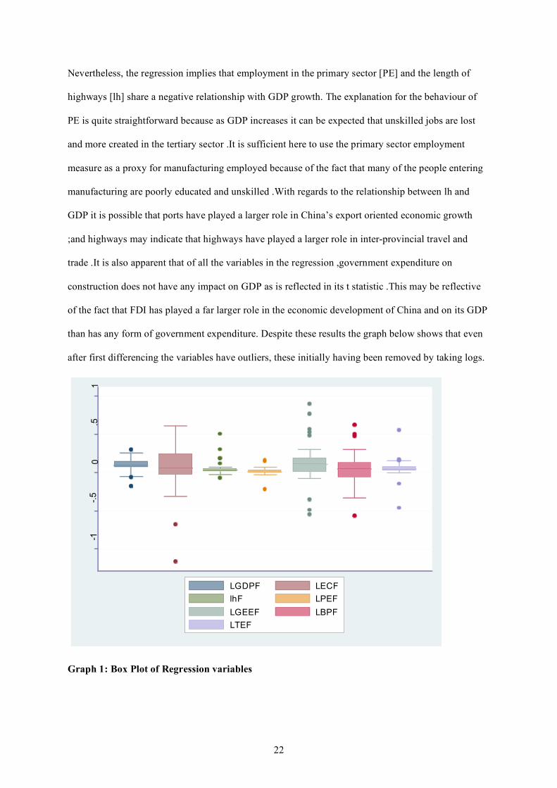
Nevertheless, the regression implies that employment in the primary sector [PE] and the length of

highways [lh] share a negative relationship with GDP growth. The explanation for the behaviour of

PE is quite straightforward because as GDP increases it can be expected that unskilled jobs are lost

and more created in the tertiary sector .It is sufficient here to use the primary sector employment

measure as a proxy for manufacturing employed because of the fact that many of the people entering

manufacturing are poorly educated and unskilled .With regards to the relationship between lh and

GDP it is possible that ports have played a larger role in China’s export oriented economic growth

;and highways may indicate that highways have played a larger role in inter-provincial travel and

trade .It is also apparent that of all the variables in the regression ,government expenditure on

construction does not have any impact on GDP as is reflected in its t statistic .This may be reflective

of the fact that FDI has played a far larger role in the economic development of China and on its GDP

than has any form of government expenditure. Despite these results the graph below shows that even

after first differencing the variables have outliers, these initially having been removed by taking logs.

-1-.5

0.5

1

LGDPF LECF

lhF LPEF

LGEEF LBPF

LTEF

Graph 1: Box Plot of Regression variables

23

It was found that even if the outliers were removed by further differencing, then the outliers removed

would only be replaced by new ones .The constant removal of outliers and differencing only added to

the reduction of the number of observations with which to carry out the analysis and thus the integrity

of the regression analysis .The consistent presence of outliers in the data, despite the use of methods

to remove them is indicative of the fact that the variables in the model follow a non-normal

distribution; and any interpretation of estimate results obtained through Ordinary Least Squares

estimation ,which focuses on the conditional mean would be misleading . Nevertheless, a method of

analysis that allows the analysis of data with a non-normal distribution [conditional median] is

Quantile Regression analysis14.The latter will provide an indication of how the mean response to

changes in the various covariates [EC, lh, PE, GEE, BP, TE] is sub-divided between the different

segments of the conditional distribution of GDP .

_cons . 0442943 . 014812 2. 99 0. 005 . 0143091 . 0742796 LTEF - . 0610443 . 1020606 - 0. 60 0. 553 - . 2676551 . 1455665 LBPF - . 015239 . 0725315 - 0. 21 0. 835 - . 1620714 . 1315934 LGEEF . 0244574 . 1121628 0. 22 0. 829 - . 2026043 . 2515191 LPEF - . 0966127 . 3147196 - 0. 31 0. 761 - . 7337291 . 5405038 lhF - . 108378 . 2221123 - 0. 49 0. 628 - . 5580209 . 3412649 LECF - . 0093257 . 0865698 - 0. 11 0. 915 - . 1845772 . 1659258 LGDPF Coef. Std. Err. t P>|t| [95% Conf. Interval] Bootstrap

.25 Pseudo R2 = 0. 4693 bootstrap( 20) SEs .50 Pseudo R2 = 0. 3129.5-.25 Interquantile regression Number of obs = 45

Table 4: Quantile Regression Results: 1952-2004

The above table shows that the lower 25% of the data set contributes significantly more to the OLS

2R than the data in any of the other percentage quantiles.

Conclusion

This paper has established that:

a) The mass relocation of people from the interior of China to the coastal region is not the only way in

which the ever widening income disparities in Chinese society can be effectively dealt with .

14 Koenker, R and Hallock, K (2001),’Quantile Regression’, The Journal of Economic Perspectives, Vol.15, No.4

24

c) Infrastructure has had a role in China’s economic development with a concentration in the

SEZ’s and HTDZ’s where export oriented economic growth has taken place taking advantage

of China’s comparative advantage over other nations in cheap labour and the most efficient

use of foreign capital .

d) Krugman’s question ,’Why does manufacturing end up being concentrated in one part of a

country leaving the other parts to a peripheral role ?’ has emerged from an existing body of

regional developmental literature to form the context of the New Economic Geography

[NEG] . However, with regards to the post 1978 economic development of China, the NEG is

out of context and needs to be modified to take into account the agglomeration economies

which result from Knowledge Creation. It is clear that not a lot of empirical work has been

done in this field and the neoclassical production function needs to be modified in a quasi-

concave additive manner to factor in agglomeration economies which arise from knowledge

creation. Furthermore, the NEG framework is abstract with regards to China’s post-reform

economic development and needs to be modified.

e) The neoclassical production function was modified and some empirical work carried out.

While, all but one of the five variables proved to be significant with regards to the impact on

GDP, the data set proved to have a non-normal distribution; and in this light Ordinary Least

Squares estimation may not be the best method of analysis.

Suggestions for further work include the in-depth use of Quantile Regression Analysis to analyse the

data; and the use of the model to analyse provincial data.

25

References

Amiti, M. and Javorcik, B.S (2005). "Trade Costs and Location of Foreign Firms in China." World Bank Policy Research Working Paper 3564(April 2005).

Bao, S., Chang, G.H, Sachs, J.D and Woo, W.T (2002). "Geographic Factors and China's Regional Development Under Market Reforms, 1978-1988." China Economic Review 13.

Barkin, D. (1972). "A Case Study of the Beneficiaries of Regional Development." International Social Development Review 4: 84-94. Bougheas, S., Demetriades.P.O, P.O and Morgenroth, E.L.W (1999). "Infrastructure, Transport Costs and Trade." Journal of International Economics 47.

Brun, J. F., Combes, J.L and Renard, M.F (2002). "Are there spillover effects between coastal and noncoastal regions of China?" China Economic Review 13: 161-169.

Caselli, F and Coleman, W.J (2006),’The World Technology Frontier’, American Economic Review, June 2006.

Chan, R. C. K. (1996). “Regional Development of the Pearl River Delta Region Under the Open Policy, Chapter 11 in "China's Regional Economic Development" edited by Chan, R.C.K et al”CUHK. Chen, J. and Fleischer, B.M (1996). "Regional Income Inequality and Economic Growth in China." Journal of Comparative Economics 22: 141-164. Demurger, S. (2001). "Infrastructure Development and Economic Growth: An Explanation for Regional Disparities in China?" Journal of Comparative Economics 29: 95-117.

Fan, S and Zhang, X (2004). "Infrastructure and Regional Economic Development in China." China Economic Review 15: 203-214.

Fleischer, B. M. and Chen, Jian (1997). "The Coast-Noncoastal Income Gap, Productivity and Regional Economic Policy in China." Journal of Comparative Economics 25.

Friedmann, J. (1966). “Regional Development Policy: A Case Study of Venezuela”. Cambridge, MIT Press. Fujita, M. and Mori, T (1996),’The Role of Ports in the Making of Major Cities: Self Agglomeration and Hub Effect ‘, Journal of Development Economics 49:93-120 Fujita, M. and Mori, T (2005), "Frontiers of the New Economic Geography." Institute of Developing Economies Discussion Paper (27).

26

Hakimi, S.L (1964),’Optimum locations of switching centres and the absolute centres and medians of a graph.’ Operations Research 12.

Hirschmann, A. O. (1958). “The Strategy of Economic Development”. New Haven, Yale University Press. Holtz-Eakin, D. and Lovely, M.E (1996). "Scale Economies, Returns to Variety and the Productivity of Public Infrastructure." Regional Science and Urban Economics 26.

Koenker, R (2005),’Quantile Regression’, Cambridge University Press

Koenker, R and Hallock, K (2001),’Quantile Regression’, The Journal of Economic Perspectives, Vol.15, No.4

Krugman, P. (1991). "Increasing Returns and Economic Geography." The Journal of Political Economy 99(3): 483-499. Krugman (1993),'On the number and location of cities’, European Economic Review 37.

Limao, N and Venables, A.J (2001),”Infrastructure, Geographical Disadvantage, Transport Costs, and Trade “, The World Bank Economic Review, Vol. 15, No 3, 451-479.

Lin, G. (1999),”Transportation and Metropolitan Development in China’s Pearl River Delta: The Experience of Panyu”, Habitat Intl, Vol.23, No.2 PP 249-270.

Luo, X. (2004). "The Role of Infrastructure Investment Location in China's Western Development." World Bank Working Paper 3345(June 2004).

Mody, A and Wang, Fang-Yi (1997). "Explaining Industrial Growth in Coastal China: Economic reforms and What Else?" World Bank Economic Review 11(2): 293-325.

Myrdal, G. (1957). “Economic Theory and Underdeveloped Regions”. London, Duckworth.

Ravallion, M. "Externalities in Rural Development: Evidence for China." World Bank Policy Research Working Paper (2879). Ravallion, M and Jalan. (1999). "China's Lagging Poor Areas." American Economic Review 89(2). Roller, Lars-Hendrik and Waverman (2001),”Telecommunications Infrastructure and Economic Development: A Simultaneous Approach”, The American Economic Review, Vol.91, No 4.

Speece, M. W. and Kawahara, Y (1995). "Transportation in China in the 1990's." International Journal of Physical Distribution and Logistics Management 25(8).

27

Spiros, B., Demetriades.P.O, P.O and Mamuneas, T.P (2000). "Infrastructure, Specialisation and Economic Growth." Canadian Journal of Economics 33(2).

Takahashi, T (2005),’Economic Geography and endogenous determination of transport technology.’ Mimeograph, University of Tokyo.