Department of Chemical Engineering

Certificate of Postgraduate Study dissertation

Multidimensional modelling of granulation

Andreas BraumannChurchill College

supervised by Dr. Markus Kraft and Dr. Paul Mort

submitted in December 2005

Preface

The work described in this report was carried out in the Department of Chemi-cal Engineering, University of Cambridge, between January and December 2005.The work is the result of my own research, unaided except as specifically acknowl-edged in the text, and it does not contain material that has already been used toany substantial extent for a comparable purpose. This report contains 7937 words.

Date Signature

AcknowledgementsI would like to thank Drs Markus Kraft and Paul Mort for their guidance through-out the year. Further thanks go to the members of the Computational ModellingGroup for several discussions and help, in particular to Mike Goodson, RobertPatterson, and Alastair Smith. Finally, I would like to thank Procter and Gambleand the University of Cambridge for funding.

AbstractThis report deals with the modelling of granulation. The mechanisms of this im-portant size enlargement process have been identified in the past, but neverthelessthere is still a lack of appropriate models. To overcome the difficulties of the pre-dictive power, a new model is proposed in the current report. The capability ofthis model is demonstrated by comparison with experimental results. In additionto this, the results of parameter studies are presented. Finally, conclusions aredrawn and an outlook on future work is given.

i

Contents1 Introduction 1

2 Literature review 12.1 Mechanisms . . . . . . . . . . . . . . . . . . . . . . . . . . . . . 22.2 Modelling of granulation . . . . . . . . . . . . . . . . . . . . . . 2

3 A new granulation model 73.1 Particle definition . . . . . . . . . . . . . . . . . . . . . . . . . . 73.2 Considered transformations . . . . . . . . . . . . . . . . . . . . . 83.3 Rates of the transformations . . . . . . . . . . . . . . . . . . . . 9

3.3.1 Addition of binder . . . . . . . . . . . . . . . . . . . . . 93.3.2 Coagulation of particles . . . . . . . . . . . . . . . . . . 103.3.3 Consolidation . . . . . . . . . . . . . . . . . . . . . . . . 143.3.4 Chemical reaction . . . . . . . . . . . . . . . . . . . . . 153.3.5 Penetration . . . . . . . . . . . . . . . . . . . . . . . . . 163.3.6 Breakage . . . . . . . . . . . . . . . . . . . . . . . . . . 16

4 Simulation results 204.1 Comparison between experiment and simulation . . . . . . . . . . 20

4.1.1 Experimental results . . . . . . . . . . . . . . . . . . . . 204.1.2 Simulation results . . . . . . . . . . . . . . . . . . . . . 23

4.2 Parameter studies . . . . . . . . . . . . . . . . . . . . . . . . . . 25

5 Summary and future work 29

References 31

Nomenclature 33

ii

1 IntroductionGranulation is an important process in industry to bring powders into a user-friendly design. In order to achieve this, liquid binder is added to small solidparticles. The particles are bound in bigger particles (granules) due to capil-lary pressure, surface tension and viscous forces (Iveson and Litster, 1998). Theprocess has numerous applications in industry ranging from mineral processingand production of fertilizers to home consumer products such as food, detergentsand pharmaceuticals. Granulation as a size enlargement process, which is alsocalled agglomeration, pelletisation or balling, has several benefits. The inclusionof small particles in bigger granules reduces the dustiness of the powder, so thatthe risks of explosions is lower than for the original powder. Furthermore, theflowability is improved, which implies better handling and easier storage. Besidesthe improvement of the handling properties of powders, granulation is also usedto create micro-mixtures of different components to prevent segregation and toachieve a desired solubility (Iveson et al., 2001; Wauters, 2001).

Different designs of equipment are established in industrial practise to performthe process. There are basically three principal ways to agitate the bulk material:in a drum, in a fluidised bed, and in a high shear mixer. Also combinations ofthese basic devices are in use such as agitated fluidised bed granulator. The shearforces tend to increase from the drum granulator towards the operation in a highshear mixer (Tardos et al., 1997).

In this report a short literature review about granulation mechanism and mod-elling will be given in section 2. This previous work has motivated the develop-ment of a new model dealing with binder based granulation. A detailed descriptionof this model is given in section 3. The capability of the new model frameworkis demonstrated by comparison with experimental results and by parameter stud-ies (section 4). Conclusions are drawn and an outline for future work is given insection 5.

2 Literature reviewAlthough one can benefit a lot from products formed by granulation, there is still alack of understanding of the entire process. Cameron et al. (2005) pointed out thatdealing with industrial particulate processes is still based on empiricism. Henceindustrial granulation plants are operated with recycle ratios of up to 5:1 (Wauters,2001; Iveson et al., 2001).

1

2.1 MechanismsNowadays the formation of granules is considered to be determined by three pro-cesses: wetting and nucleation, coalescence and consolidation, and attrition andbreakage (Iveson et al., 2001). The process of wetting and nucleation includesthe addition of liquid binder to the particle bed and the coalescence of the dropletwith solid particles, so that nuclei are formed. These wetted particles are able tocoalesce with other particles. A detailed investigation of nucleation and binderdispersion can be found in the thesis of Hapgood (2000).

Granulation is ultimately carried out because we are interested in the benefi-cial process of coalescence. Depending on the conditions, surface wet particlesstick together and form bigger particles (granules). The reduction of pore vol-ume of the granules is referred to as consolidation, or compaction. It is causedby inter-granule and granule-equipment collisions (Iveson et al., 2001). Fric-tional, viscous, elastic, and capillary forces act against consolidation (Iveson etal., 1996).

Attrition and breakage act as contrary processes to coagulation. Essentiallyattrition and breakage refer to the same process, namely the destruction of a parentparticle and thus the generation of a broken/abraded parent particle and (new)daughter particles. In the case of attrition, the size of the parent particle hardlychanges, and the separated daughter particles are small. Breakage, sometimes alsocalled fragmentation, leads to the creation of fragments which are in the same sizerange as the parent particle (Ouchiyama et al., 2005).

These processes, which are considered to control the outcome of the granula-tion process, must be seen in connection with other processes which also have aninfluence on the final product quality. According to Mort and Tardos (1999) theseprocesses include: mixing of the powder feeds, binder atomisation, and chemicalreactions between binder and solids, to name but a few. Even drying as a postprocess of agglomeration should be taken into account during the design of thegranulation process.

2.2 Modelling of granulationKapur and Fuerstenau (1969) were amongst the first to attempt to model the gran-ulation process. They assumed random coalescence between all particles, whichmeans that the likelihood of a successful coalescence of two particles is always thesame irrespective of their sizes or other physical properties. At time zero the par-ticle distribution is assumed to be monodisperse. Experiments with a limestone-water-system have been carried out to test the model. Compaction was observedduring the course of the experiments, so that granule sizes have been measuredto correct the predicted particle sizes. This means that the predictions have been

2

adapted to the experimental results. Despite this significant drawback, the workpresents an interesting attempt to model granulation.

Each particle of an ensemble can be characterised according to a number ofproperties. By observing the frequency of particles with a given property, wecan derive the corresponding particle distribution (e. g. particle size distribution,binder distribution). In order to model the evolution of these particle ensembles,we construct suitable population balance equations (Ramkrishna and Mahoney,2002).

The general structure of the population balance equation for the number den-sity function f takes following form (Cameron et al., 2005):

∂f(~r, ~x, t)

∂t=∇r · ∇r [Drf(~r, ~x, t)]︸ ︷︷ ︸

geometric diffusion

−∇r · R f(~r, ~x, t)︸ ︷︷ ︸geometric convection

− ∇x · X f(~r, ~x, t)︸ ︷︷ ︸convection along

property coordinates

+ σ(~r, ~x, t)︸ ︷︷ ︸source/sink

,(1)

where ~r is the vector of the geometric (or external) coordinates, ~x is the vector ofthe internal or property coordinates, and R and X are the velocity vectors for therespective coordinates. The change in the number density function f(~r, ~x, t) withrespect to time t is determined by dispersion and convection along the externalcoordinates, convection along the internal coordinates, and by any sources andsinks. The important processes of coalescence and breakage (qv. section 2.1) areconnected to eq. (1) via the source and sink term. The application of populationbalances is not restricted to granulation, rather they are widely used in chemicalengineering ranging from crystallisation and precipitation to polymerisation andthe analysis of biological populations (Ramkrishna and Mahoney, 2002).

Equation (1) is quite complex, so in order to proceed it is necessary to makecertain simplifying assumptions. In particular, the spatial dependency of the num-ber density function f is often neglected. This means that the process must be abatch process with the same number density function at every geometric point. Ifthe vector of the internal coordinates ~x is reduced to a single coordinate x, whichmay be the particle size, then the scalar equation (1) simplifies to

∂

∂tf(x, t) = − ∂

∂x

(dx

dtf(x, t)

)+ σ(x, t) . (2)

For the case of coagulation only, eq. (2) becomes the Smoluchowski coagulation

3

equation (von Smoluchowski, 1916):

∂

∂tf(x, t) =

1

2

∫ x

0

K(x− y, y) f(x− y, t) f(y, t) dy

−∫ ∞

0

K(x, y) f(x, t)f(y, t) dy . (3)

The first term accounts for the creation of particles of size x due to coagulationof particles of size x − y and y. The kernel K determines the rate of coagula-tion. The second term accounts for the disappearance of particles of size x due tocoagulation with particles of size y.

Equation (3) has been used to model different granulation processes (Kapurand Fuerstenau (1969); Adetayo et al. (1995); Wauters (2001)), but the kernel hasalways had an empirical or semi-empirical form. The problem with these sorts ofkernels is that they are only valid in the range for which the fit has been made.To overcome this deficiency, various efforts have been made to derive physicallybased kernels during the last decade. A list of available models can be foundin Iveson et al. (2001). The models can be divided into two classes. Modelsof the first class assume that coalescence is successful if the kinetic energy ofthe particles can be dissipated during the collision of the particles. In contrastto this, the models of the second class are based on the assumption that granulesare formed if the bonds between the colliding particles are large enough to resistfollowing collision or shear forces which would lead to the breakage of the bond.

There is clear evidence that population balances with only one dimension, i. e.one internal coordinate, are not sufficient to model granulation processes. Thisfinding can be explained by the fact that granules consists of more than one com-ponent (at least one solid material and one binder). Hence particles must be de-scribed by more than one independent variable, because the granulation behaviourstrongly depends on particle properties like granule size, porosity, binder con-text, and composition (Iveson, 2002). The same conclusions have been drawn byWauters (2001). He proposed a model which described a particle by its solid vol-ume, liquid volume, and volume of air. These particles underwent the processescoalescence and compaction. The coagulation kernel K used is semi-empirical,and he made use of the fact that the kernel can be split into two parts:

K(~x, ~x′) = K0 K(~x, ~x′) (4)

with ~x and ~x′ being the vectors of the independent variables of the two collid-ing particles. The rate constant K0 lumps the various system parameters such asoperating conditions and material properties. The term K(~x, ~x′) gives the proba-bility of a successful coalescence of the two particles, and has been been derivedfrom experiments. According to observations from the experiments, the particles

4

are categorised into small/large and dry/wet. The distinction between small andlarge particles is made, because a stage with slow particle growth and a followingstage with rapid growth was recognised. Once the small particles are “collected”by the bigger granules, faster growth occurred. However, coalescence can onlyoccur if the particles are surface wet, hence it was assumed that the liquid (binder)is covered inside the particles until a critical value of liquid amount to air vol-ume is exceeded. This ratio was also derived from the experiments. Combiningthe categories small/large and dry/wet leads to coalescence probabilities for eachcombination with either K(~x, ~x′) = 1 for successful coagulation or K(~x, ~x′) = 0for a collision of particles which does not result in a new particle. Compactionof the particles is dealt with by the approach of Iveson et al. (1996). The changeof the particle porosity ε with respect to the time t (or equivalently the number ofdrum revolutions) is given by:

dε

dt= −k (ε− εmin) . (5)

The rate constant k and the minimum granule porosity εmin are functions of theoperating conditions and material properties. Wauters (2001) concludes that thesimulation results using the model with the multidimensional particle descriptionare in agreement with his experimental results. Consequently he concludes that“the multi-dimensional population balance has great potential for modelling gran-ulation processes”.

Goodson et al. (2004) presented a new model. As in the work of Wauters,three independent variables are used to describe a particle. Since the particle de-scription of Wauters (2001) with the air volume as an independent variable canlead to unphysical results (negative air volume) due to the compaction, Goodsonet al. (2004) used the solid volume, the surface area, and the liquid amount as inde-pendent variables. They considered the processes of coagulation and compactionin their model. In addition to the particle categories small/large and wet/dry athird category hard/soft was introduced. This is explained by the fact that duringthe coalescence of particles new void volume can be enclosed. The amount ofnew pore volume depends on the hardness of the particles which is characterisedby the porosity. Therefore two extremes have to be considered. If both particlesare hard, then the total surface area is conserved (increase of total volume). Inthe other case, i. e. the collision of two soft particles, it is assumed that the totalvolume of both particles is conserved. This means that the total surface area de-creases. Compaction of the particles is also dealt with by the approach of Ivesonet al. (1996). As a result it is shown that this new model is capable of predictingthe outcome of the granulation process. The simulation results are confirmed byexperimental results.

The equations which arise from the modelling can become quite complex.

5

Only in very simple cases is it possible to solve these equations analytically. Inmost circumstances it is necessary to apply numerical methods to get a solutionof the models, because the population balance equations are integro-differentialequations. One possibility to solve the equations is obtained by discretisationalong the internal coordinate(s). There can be a drawback due to a fixed discreti-sation, so that methods with finer and coarser grid or even adaptive grid size havebeen developed (Cameron et al., 2005). According to Ramkrishna and Mahoney(2002) finite element approaches have the drawback that the effort to obtain a so-lution for models grows exponentially with the number of dimensions. To avoidthese problems, one may use a Monte Carlo method to solve the equations of thegranulation model. For this sort of problem it seems to be desirable to choose adirect simulation algoritm among the Monte Carlo methods, because the particlesof the real system can be represented by a smaller number of simulation particles(Smith and Matsoukas, 1998; Kruis et al., 2000). Further information about thedirect simulation algorithm can be found in Goodson and Kraft (2004).

Patterson et al. (2004) did further development of the direct simulation algo-rithm. The outcome of this development is the so called Linear Process DefermentAlgorithm. Basically this algorithm is still a direct simulation algorithm, but thecomputational time needed to solve these equations is cut down significantly. Thisreduction can be achieved by the deferment of linear processes. This means thatthe changes due to the deferred processes are calculated less often. The accuracyof the algorithm is influenced by the length of the deferment step.

As a summary of this section, it can be stated that:

1. Some modelling of granulation processes has been done in the past.

2. One-dimensional population balances are not sufficient to describe the pro-cess. It is necessary to describe the particles by several independent vari-ables.

3. Coalescence is an important process during granulation. Hence the choiceof kernel used for the model is crucial. This means with an improved de-scription of the particles, physically based coagulation kernels should beused.

4. Further attention should be paid to processes other than coalescence andcompaction, like wetting, breakage, and chemical reactions.

5. To solve the complex model equations, Monte Carlo algorithms seem to bea good choice.

As the former models have certain limitations for the description of granula-tion processes, a new model has been developed and is presented in section 3.

6

3 A new granulation model

3.1 Particle definitionParticles can be described by any number of properties. As in former models, theparticle size is certainly an important property. But it can be derived, once thecomposition of a single granule is known. This becomes an important point whenmicro-mixtures are considered or properties such as the dissolution behaviour arethe focus of the application. Hence, the single components of each granule aretracked in the forthcoming model.

The volume of the original solid is the first component to be considered for thedescription of granules. To make granulation happen, liquid binder on the surfaceof the particles is needed, so that the external liquid volume is the second particleproperty to be tracked. Pores/pore volume will be created due to the coalescence.These pores are at least partly occupied by binder which shall be accounted forby the volume of internal liquid. As mentioned in section 1, chemical reactionscan occur so that new substances are formed. This volume of reacted solid isalso a property of the granules which has to be tracked. The shape of a particleis assumed to be spherical. In total, a particle is described by five independentvariables. From these it is possible to express other properties such as the totalvolume (particle size) or the surface area. Table 1 summarises the variables thatdescribe a particle.

Table 1: Variables describing a particle

dependency variable notation unitindependent original solid volume so m3

reacted solid volume sr m3

external liquid volume le m3

internal liquid volume li m3

pore volume p m3

dependent total volume v m3

external surface area ae m2

internal surface area ai m2

porosity ε -

7

The vector ~x of internal coordinates (independent variables) therefore has theform:

~x = (so, sr, le, li, p) (6)

and is an element of the type space E (~x ∈ E). The derivatives of ~x with respectto time t give the vector of the velocities along the internal coordinates

X =

(dso

dt,dsr

dt,dledt

,dlidt

,dp

dt

). (7)

There exists relationships between the different variables, which are summarisedin the following equations. The total particle volume v is obtained by

v = so + sr + le + p . (8)

As the particle is a sphere, the external surface area ae can be derived from thetotal volume v,

ae = π1/3 (6 v)2/3 . (9)

The internal surface area is considered to be proportional to the pore volume,

ai = C p2/3 with C > π1/3 62/3 ≈ 4.836 , (10)

and the porosity ε becomes

ε =p

v. (11)

3.2 Considered transformationsThe particle ensemble changes during the granulation process due to transfor-mations taking place, i. e. events and mechanisms. Using the considerations pre-sented in the literature (see section 2.1), the following transformations are defined:

1. Addition of binder

2. Coagulation of particles

3. Consolidation (porosity reduction)

4. Chemical reaction on the (internal and external) surface

8

5. Mass transfer of liquid into the pores (penetration): external liquid becomesinternal liquid

6. Breakage/attrition

If it is assumed that the particle ensemble is well mixed and the process isconsidered to be a batch process with no outflow, then the population balancetakes the following form:

∂

∂tf(~x, t) =−∇x · X f(~x, t)

+1

2

∫∫~y, ~z ∈E2

1{y+z=x} K(~y, ~z) f(~y, t) f(~z, t) d~y d~z

− f(~x, t)

∫~y ∈E

K(~y, ~x) f(~y, t) d~y

+

∫ ∞

~x

b(~y, ~x) g(~y) f(~y) d~y

− g(~x) f(~x, t)

+ I f in(~x, t)

(12)

The first term on the right hand side accounts for continuous changes of the par-ticles. This might be caused by crystal growth in a crystallisation process or achemical reaction. The second and third terms describe the generation of parti-cles with the properties ~x and the removal of these granules due to coagulation.Furthermore, eq. (12) includes terms for the breakage of particles (fourth and fifthterm on the RHS). To describe this process, it is necessary to know the breakagefrequency g, which gives a measure how often a particle is broken. The break-age process leads to the creation of smaller particles (daughter particles) whosedistribution is given by the breakage function b(~y, ~x). This function defines howmany particles with the properties ~x arise due to the breakage of a granule withthe properties ~y. The last process accounted for in eq. (12) is the inception of par-ticles. This process is characterised by the inception rate I and the number densityfunction of the added particles f in.

3.3 Rates of the transformations3.3.1 Addition of binder

To achieve a good distribution of binder on the particle, the binder (liquid) is usu-ally sprayed into the granulator through a nozzle. This means that small dropletsare added to the existing particle ensemble. Thus, these droplets can be described

9

by the particle definition, because they are only a special case of “real” particles.The vector of independent variables for a droplet becomes

~xdroplet = (0, 0, le, 0, 0) . (13)

The addition of binder is determined by the flow rate Vl and the droplet size dis-tribution pin, which is the normalised number density of the droplets. This distri-bution is a characteristic of each nozzle and must be obtained by measurement.With these known parameters the term I f in(~x) in eq. (12) can be expressed as

I f in(~x) =Vl

Vreactor

pin(~x)∫~x∈E

~x pin(~x) d~x

. (14)

3.3.2 Coagulation of particles

The coagulation rate is determined by the coagulation kernel K(~x, ~x′) of the twocolliding particles with the properties ~x and ~x′ respectively. Recall that it can besplit into two parts

K(~x, ~x′) = K0 K(~x, ~x′) . (4)

The term K0 is independent of the properties of the two colliding particles andlumps the general conditions. The term K accounts for the probability of a suc-cessful coalescence and becomes either 1 (successful collision) or 0 (unsuccessfulcollision). Wauters (2001) and Goodson et al. (2004) categorised the particleswith respect to two and three properties respectively and for the combinationsthereof. These categorisations were used to define whether a collision of twoparticles leads to coalescence or not. To overcome the difficulties of categoris-ing particles, a physical based criterion has been chosen for the current model todecide whether a new granule results from the collision of two particles. ThisSTOKES criterion has been proposed by Ennis et al. (1991). According to thiscriterion, a collision leads to coalescence if the kinetic energy of the two collidingparticles is dissipated in the viscous binder layer. The solution of the momentumbalance (Ennis et al., 1991) leads to the viscous STOKES number Stv:

Stv =collision energy

energy of viscous dissipation=

m U

3 π η R(15)

with m = harmonic mean granule massU = collision velocity

( = relative velocity between the two particles)η = binder viscosity

R = harmonic mean particle radius .

10

The particle radius R and mean mass m have to be calculated as followed:

R =2 Rj Rk

Rj + Rk

, (16)

m =2 mj mk

mj + mk

, (17)

where the radius R and granule mass m can be obtained by

R =3

√3 v

4 π, (18)

m =∑all i

mi , (19)

which can be simplified with the assumption that ρsr = ρli = ρle to

m = ρso so + ρle (sr + li + le) . (20)

Coagulation takes place if the critical STOKES number St∗v is bigger than the vis-cous STOKES number St∗v.

Stv 6 St∗v : K = 1 : coalescence

Stv > St∗v : K = 0 : no coalescence .(21)

The critical STOKES number St∗v is defined by:

St∗v =

(1 +

1

ecoag

)ln

(h

ha

)(22)

with ecoag = coefficient of restitutionh = thickness of binder layerha = characteristic length scale of surface asperities .

The thickness of the binder layer h should be defined as the combined binderthickness of both particles (j, k),

h =hj + hk

2, (23)

with the thickness of the binder layer of a particle calculated by

h =1

23

√6

π

[3√

v − 3√

v − le

]. (24)

11

The coefficient of restitution in eq. (22) is defined as the geometric average of thecoefficients of restitution of the single particles (j, k),

ecoag =√

ej · ek . (25)

A mass-weighted arithmetic average is used for the calculation of the coefficientof restitution e of each particle core.

e =

∑all i 6= le

ei mi∑all i 6= le

mi

. (26)

The coefficient of restitution e is the ratio of rebound energy to impact energy, andhence it takes values between zero (totally plastic impact) and one (totally elasticimpact). For a first guess it is assumed that eso = 1, esr = 1, ele = 0, and eli = 0and it is kept in mind that ρsr = ρle , which yields

e =

0 , v = le

ρso so + ρle sr

ρso so + ρle (li + sr), otherwise .

(27)

If the two particles (j, k) coalesce, the properties of the new particle are calculatedas followed:

so = so,j + so,k , (28)sr = sr,j + sr,k , (29)le = le,j + le,k − le→i,j − le→i,k , (30)li = li,j + li,k + le→i,j + le→i,k . (31)

In equation (30) and (31) it is taken into account that a certain amount of externalliquid becomes internal liquid due to the coagulation. Figure 1 illustrates thearrangement of the particles immediately before the coalescence with the volumesle→i,j and le→i,k. With the situation shown in fig. 1, le→i,j can be computed by thefollowing expression:

le→i,j =le,j2

1−

√√√√1−

(3√

vk − le,k3√

vj + 3√

vk

)2 (32)

By changing the indices, the previous equation can be applied to the other particleas well. But, for high ratios (vk − le,k)/(vj − le,j), eq. (32) can lead to physically

12

le→i, j le→i, kvk

vj

le, j

le, k

Figure 1: Transformation of external liquid to internal liquid due to coalescenceof two particles

unreasonable results. Thus, a reduced internal volume of the particles vi is definedas

vi =√

(vj − le,j) · (vk − le,k) , (33)

so that le→i,j becomes

le→i,j =le,j2

1−

√1−

(3√

vi

3√

vj + 3√

vk

)2

=le,j2

1−

√√√√1−

(6√

(vj − le,j) · (vk − le,k)3√

vj + 3√

vk

)2

(34)

and

le→i,k =le,k2

1−

√1−

(3√

vi

3√

vj + 3√

vk

)2

=le,k2

1−

√√√√1−

(6√

(vj − le,j) · (vk − le,k)3√

vj + 3√

vk

)2 .

(35)

The external surface area and the pore volume of the new granule depend on thesoftness of the two former particles. The coefficient of restitution ecoag, which is

13

a measure of the softness of the particles, has been introduced in eq. (25) and cannow be used for the calculation of the external surface area of the new formedgranule:

ae = (1− ecoag)(a

3/2e,j + a

3/2e,k

)2/3

︸ ︷︷ ︸soft

+ ecoag (ae,j + ae,k)︸ ︷︷ ︸hard

. (36)

This approach is similar to the one proposed by Goodson et al. (2004). The porevolume of the newly formed particle can be derived from eqs. (8) and (9)

p =a

3/2e

6√

π− so − sr − le . (37)

3.3.3 Consolidation

Each collision of particles leads to consolidation and will be described by anadapted approach using the findings of Iveson et al. (1996). This means con-solidation is considered to be a subevent of coagulation and shall happen in thecurrent model irrespective of whether coalescence is successful or not. The ap-proach of Iveson et al. (1996) uses an empirical model which predicts the averageporosity of a particle ensemble. For the time being, it is assumed that this ap-proach can be followed for single particles too, so that the porosity change ∆εdue to particle collision is described by:

∆ε =

{kporred U (ε− εmin) , if ε−∆ε > εmin

0 , otherwise(38)

with kporred = rate constant of porosity reductionU = collision velocityεmin = minimum porosity (depends on material properties)

Internal liquid is squeezed onto the external surface if the porosity after consoli-dation, ε′, is smaller than the critical porosity, ε∗, which is achieved when the porevolume is totally occupied by internal liquid (li = p),

ε∗ =li

so + sr + le + li. (39)

Equation (39) allows the distinction between two cases, the non-squeezing caseand the squeezing case. We let unprimed variables denote the state before consol-idation and primed variables denote the state after consolidation, so that

ε′ = ε−∆ε . (40)

14

Non-squeezing case (ε′ > ε∗) If no internal liquid is squeezed onto the externalsurface, only the pore volume (as independent variable) changes.

s′o = so, s′r = sr, l′e = le, l′i = li , (41)

p′ =ε′

1− ε′(s′o + s′r + l′e) . (42)

Squeezing case (ε′ 6 ε∗) Although liquid is transferred from the interior of theparticle onto the external surface, the total amount of liquid remains constant.

s′o = so, s′r = sr , (43)p′ = l′i = ε′ (s′o + s′r + le + li) , (44)l′e = le + li − l′i . (45)

3.3.4 Chemical reaction

Unless the components of a granule are totally inert, chemical reactions have to beconsidered. Rules for the transformation of liquid into reacted solid are given asfollows. The reaction of external and internal liquid are dealt with separately. Therespective reaction rate rreac shall be dependent on the surface area a of the con-sidered region of the granule. Hence the reactions rates are described by followingequations

Reaction on the external surface:

rreac,e =

kreac,e aele

le + sr

, if so > 0 and le > 0

0 , otherwise(46)

Reaction on the internal surface:

rreac,i =

kreac,i aili

li + sr

, if so > 0 and li > 0

0 , otherwise .

(47)

Due to the reactions the particles become harder as the coefficient of restitutionchanges. The amount of external liquid will be reduced so that coalescence is lesslikely. Furthermore, the conversion of internal liquid into reacted solid leads toa reduction of the pore volume/porosity. In the current case, these reaction ratesare simple, but in general any conceivable reaction can be defined in the model.

15

As the densities for external and internal liquid, and the reacted solid are the same(ρle = ρli = ρsr), the changes of the internal coordinates are obtained by

dso

dt= 0 , (48)

dsr

dt= rreac,e + rreac,i , (49)

dledt

= −rreac,e , (50)

dp

dt=

dlidt

= −rreac,i . (51)

3.3.5 Penetration

A liquid droplet which coalesces with a “real” particle will increase the amountof external liquid of the new particle. If this particle is porous, external liquidwill probably penetrate into the pores. To deal with this process, the followingequation for the penetration rate rpen is proposed:

rpen = kpen le (p− li) . (52)

The penetration rate rpen is proportional to the amount of external liquid le anddepends also on the remaining empty pore volume (p− li). The rate law is rathersimple for the moment, but as before there are no restrictions on the incorpora-tion of a more complicated law in the future. The changes of the independentproperties of a granule due to penetration are given by

dso

dt= 0,

dsr

dt= 0 , (53)

dledt

= −rpen , (54)

dlidt

= rpen , (55)

dp

dt= 0 . (56)

3.3.6 Breakage

There is still a lack of modelling breakage in granulation, although it has beenidentified to be a significant process in high shear and drum granulation (Cameronet al., 2005). Fu et al. (2005) performed experiments in order to investigate thebreakage behaviour of single wet granules, but a model was not derived. As thereexists no general description of the breakage of wet granules which takes care of

16

the operating conditions, the material properties, and the granule properties, ourapproach is presented in this section.

For the characterisation of a breakage process, the likelihood of breakage ofany particle and the properties distribution (e. g. size distribution) of the newlyformed particles have to be known. The likelihood of breakage is described bythe breakage frequency g(~x). The breakage frequency is seen to be proportionalto the particle volume v. Iveson et al. (2001) mentions that granules with highporosity are weak. This means that the probability of their breaking should behigher than for less porous particles. The granules are covered by external liquidon the outer surface. It is expected that a particle with a considerable amount ofexternal liquid is weaker than a particle without it. These considerations lead tothe breakage frequency of a particle with the properties ~x and is calculated by thefollowing equation:

g(~x) =

katt (ε + χ) v , if v >νmin,max

νmax

vfrag,min

0 , otherwise, (57)

with ε =p

v=

p

so + sr + le + p,

χ =lev

.

Formulation (57) also enables the breakage of pure droplets (χ = 1).Further the distribution of the fragments is needed. Therefore, the probability

density fatt of the abraded daughter particles is modelled with a beta distribution.The volume of a fragment will be in the range [vfrag,min; vfrag,max] and depends onthe material properties and loading conditions.

fatt(Θ) =1

B(a, b)Θa−1 (1−Θ)b−1 with B(a, b) =

∫ 1

0

Θa−1 (1−Θ)b−1 dΘ

(58)

The skewness of the graph is determined by the parameters a and b. The graphof the distribution is symmetric for a = b and becomes skewed as a differs fromb. For the use of the beta distribution in the described model, the variable Θ isdefined as followed:

Θ =vfrag − vfrag,min

vfrag,max − vfrag,min

, (59)

where vfrag denotes the total volume of the new fragment. The minimum fragmentsize is a constant value for all parent particles, whereas the maximum fragmentsize is dependent upon the total volume of the parent particle according to

vfrag,max = νmax vparent (νmax 6 0.5) . (60)

17

νmax is constant for all particles and characterises whether breakage or attrition ismore likely in the system. The definition (60) assumes that all particles behave inthe same way irrespective of their size and other properties like the porosity. Asthe maximum fragment size can not be smaller than the minimum fragment size,a further constraint has to be introduced, namely that

vfrag,max > νmin,max vfrag,min (νmin,max ∈ [1;∞)) . (61)

The combination of eq. (60) and (61) gives a definition of the smallest parentparticle that can be broken,

vparent,min =νmin,max

νmax

vfrag,min . (62)

For the further treatment of the breakage problem it is assumed that the processhas binary character. This means that breakage of a particle leads to a daughterparticle and the remaining parent particle.

After the size of a daughter particle has been chosen, it is still necessary todetermine its composition, which may or may not be the same as that of the parentparticle. Because of the external liquid on the outer surface of the parent particle,one might imagine that the daughter particle has a higher fraction of externalliquid than the parent particle. To allow for an unequal distribution of the externalliquid, the variable κ is introduced and defined as followed:

κ =le

p + le. (63)

The parameter κ of the daughter particle can be chosen as

κfrag = κ1/nparent (n > 1) . (64)

The relationship between κfrag and κparent with its dependency on the parametern is shown in fig. 2. An increasing parameter n leads to daughter particles whoserelative amount of external liquid is higher than that of the parent particle. Forthe calculation of the properties of the daughter particle it is useful to considerdifferent cases. If the parent particle is non-porous (ε = 0), the particle can eitherbe a “real” particle with a completely solid core which is covered by externalliquid or the particle can be a droplet (v = le). As breakage of non-porous particleswithout external liquid is not allowed (eq. (57)), only external liquid should betransferred to the daughter particle in either of the cases. Hence the compositionof the daughter particle for the case κfrag = 1 is as followed:

so,frag = 0, sr,frag = 0, pfrag = 0 , (65)le,frag = v, li,frag = 0 . (66)

18

0 0.2 0.4 0.6 0.8 10

0.2

0.4

0.6

0.8

1

κparent

[−]

κ frag

[−]

n←

n=1

n=1.0n=1.5n=2.0n=2.5n=3.0n=3.5

0 0.2 0.4 0.6 0.8 10

0.2

0.4

0.6

0.8

1

κparent

[−]

κ frag

[−]

n←

n=1.0n=1.5n=2.0n=2.5n=3.0n=3.5

Figure 2: Relation between κ of the daughter and parent particle in dependenceof the parameter n (eq. 64)

For any other cases (κfrag < 1) it is assumed, that the composition of the “solidcore” (so, sr, li, p) of the daughter particle is the same as for the parent particle.The composition of the daughter particle can be calculated by following equa-tions:

pfrag = vfrag

(p

so+sr+p

)parent

1 +κfrag

1−κfrag

(p

so+sr+p

)parent

, (67)

le,frag =κfrag

1− κfrag

pfrag (6 le,parent) , (68)

so,frag =

(so

so + sr + p

)parent

· (vfrag − le,frag) , (69)

sr,frag = (v − le − so − p)frag , (70)

li,frag =

(lip

)parent

· pfrag . (71)

This section gives a complete description of the granulation process to be mod-elled. The particles are described by five internal coordinates (properties). The sixdifferent processes that can happen in the system have been defined. The rates ofthese processes have been modelled.

The model is used in section 4 to simulate a granulation process.

19

4 Simulation resultsThe complexity of this new model (introduced in section 3) makes it necessary toappel to numerical methods in order to solve the resulting equations. To obtain asolution for the five dimensional model, a Monte Carlo method is applied. Simu-lations using the Linear Process Deferment Algorithm were performed to comparethe model with experimental results and to show the influence of selected modelparameters on the outcome of the granulation process.

4.1 Comparison between experiment and simulationExperiments have been performed by the industrial partner Procter and Gamble inorder to test the capability of the new model. In the experiments sodium carbonateparticles were granulated with an aqueous PEG-4000 solution used as binder in abench scale high shear mixer.

In the past it was usual to track only the particle size as the characteristic of theparticles. As the granulation model considers also the composition of the parti-cles, it is desirable to measure other attributes of the granules too. One importantfeature is the amount of binder in a particle. To determine this characteristic,the binder was traced with a blue pigment and optical measurements were per-formed at different times throughout the process. The amount of reflected bluelight was measured, which is an indicator of the binder amount/coating level, be-cause the binder contains blue pigment. The light reflection was measured as anRGB composition so that a non-coated/white particle reflects red, green, and bluelight equally.

4.1.1 Experimental results

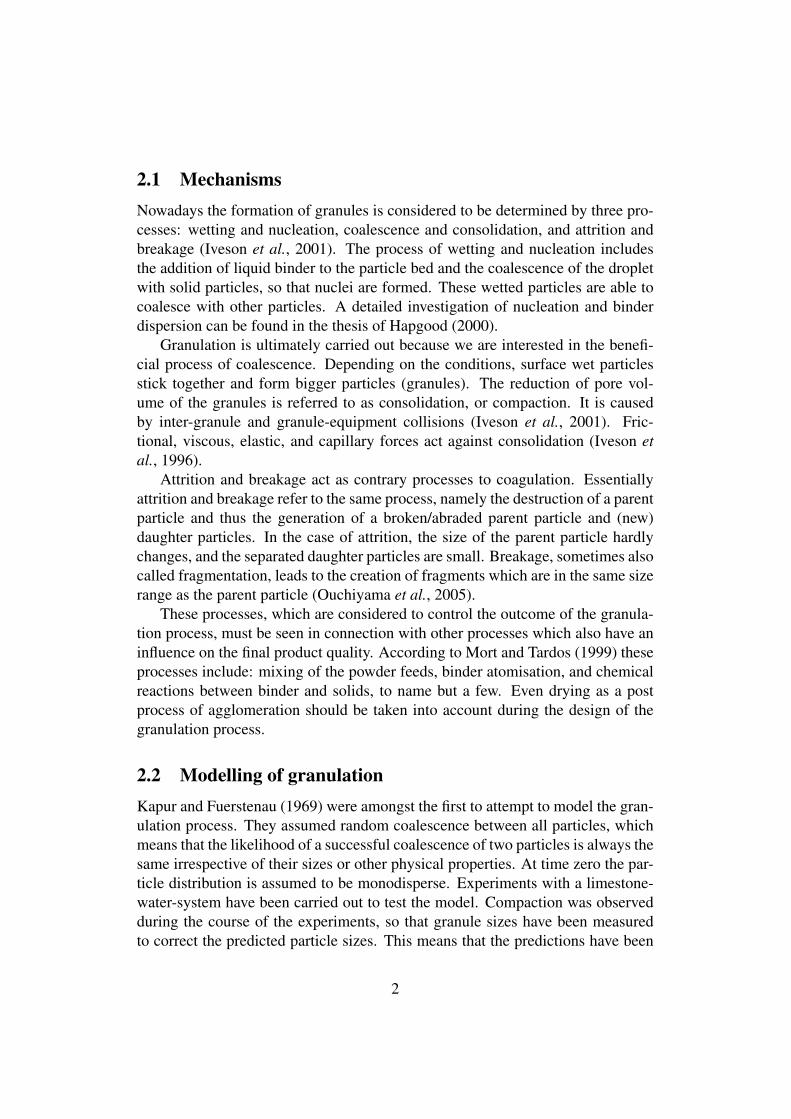
The experiment started with a dry feedstock of non-porous particles. The nor-malised number and volume density functions of the feedstock are shown in fig. 3.

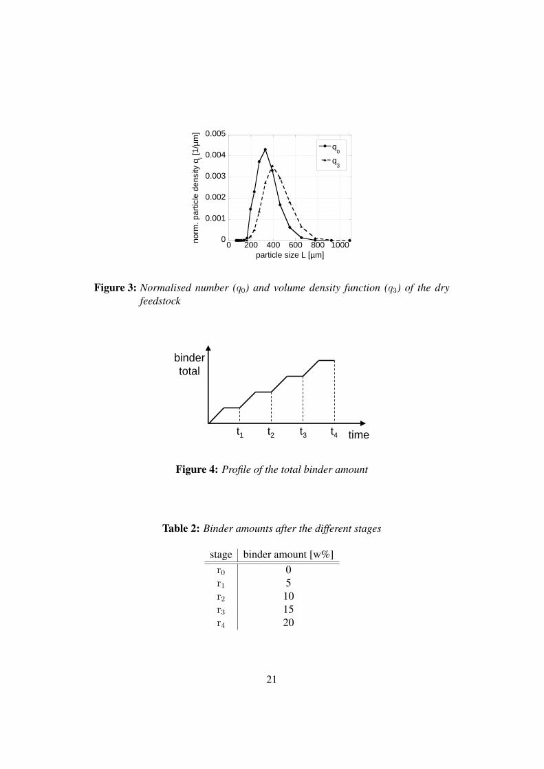
The granulation was performed in four equally timed stages. During the firsttwo-thirds of each stage binder was added with a syringe, whereas for the rest ofthe stage no binder addition took place so that a profile of the total binder amountsuch as in fig. 4 emerged. Table 2 summarises the binder amounts which areobtained after every stage.

When the stage time was over, the mixer was switched off and a sample wastaken to measure the size and the binder amount/coating level of the particles.The results of the particle measurements after each stage are shown in fig. 5. Theparticle distributions are plotted as a function of the particle size and the coatinglevel in terms of the percentage of blue light reflected (%B). The addition of binder

20

0

0.001

0.002

0.003

0.004

0.005

0 200 400 600 800 1000

q0

q3

norm

. par

ticle

den

sity

qi [1

/µm

]

particle size L [µm]

Figure 3: Normalised number (q0) and volume density function (q3) of the dryfeedstock

t1 t2 t3 t4 time

bindertotal

Figure 4: Profile of the total binder amount

Table 2: Binder amounts after the different stages

stage binder amount [w%]r0 0r1 5r2 10r3 15r4 20

21

particle size [µm]

%B

[−]

0 500 1000 1500 2000

33

36

39

42

45

0.2

0.4

0.6

0.8

1

1.2

1.4

1.6

1.8x 10

−3

(a) At the start (r0), 0 w% binder amount (dry particles)

particle size [µm]

%B

[−]

0 500 1000 1500 2000

33

36

39

42

45

2

3

4

5

6

7

8

9

x 10−4

(b) After r1, 5 w% binder amount

particle size [µm]

%B

[−]

0 500 1000 1500 2000

33

36

39

42

45

1

2

3

4

5

6x 10

−4

(c) After r2, 10 w% binder amount

particle size [µm]

%B

[−]

0 500 1000 1500 2000

33

36

39

42

45

1

1.5

2

2.5

3

3.5

4

4.5

5x 10

−4

(d) After r3, 15 w% binder amount

particle size [µm]

%B

[−]

0 500 1000 1500 2000

33

36

39

42

45

1

1.5

2

2.5

3

3.5

4

4.5

x 10−4

(e) After r4, 20 w% binder amount

Figure 5: Normalised volume-binder amount-densities of the experiments (r0–r4)

22

300

400

500

600

700

800

r0 r1 r2 r3 r4stage

part

icle

siz

e [ µ

m]

mean size

Sauter-diameter

Figure 6: Volume mean size and Sauter-Diameter of the measured particle sizedistributions after the different stages of the experiment

causes an increase of the reflected blue light, however significant growth of theparticles can be noticed at a binder amount greater than 5 w%. This observationis confirmed by a plot of the volume mean size and the Sauter-diameter (fig. 6).

4.1.2 Simulation results

The experimental results from the previous section are now compared with simu-lation results. Lots of rate constants and material properties are contained in themodel, which are not all known. Further investigations and measurements arerequired to determine these parameters. But for the time being, unknown valuesare just estimated. The predicted evolution of the granulation process is shown infig. 7. We refer to this simulation in subsequent considerations as the ‘referencecase’.

The simulation results also allow the volume mean size and Sauter-diameterto be deduced. A comparison for both of these characteristics of the particle en-semble is made in fig. 8. From the previous figures it can be concluded that thereis close agreement between the trends of the experiment and the simulation (refer-ence case). The characteristic particle sizes of the simulation are of the right orderof magnitude, although there is a remarkable deviation between experiment andsimulation for the r2 stage. The model gives a correct qualitative prediction of theprocess evolution.

23

particle size [µm]

volu

me

frac

tion

bind

er [−

]

0 500 1000 1500 2000

0.2

0.3

0.4

0.01

0.015

0.02

0.025

0.03

0.035

0.04

0.045

0.05

(a) After r1

particle size [µm]

volu

me

frac

tion

bind

er [−

]

0 500 1000 1500 2000

0.2

0.3

0.4

0.03

0.04

0.05

0.06

0.07

0.08

0.09

0.1

0.11

(b) After r2

particle size [µm]

volu

me

frac

tion

bind

er [−

]

0 500 1000 1500 2000

0.2

0.3

0.4

0.02

0.03

0.04

0.05

0.06

0.07

0.08

0.09

(c) After r3)

particle size [µm]

volu

me

frac

tion

bind

er [−

]

0 500 1000 1500 2000

0.2

0.3

0.4

0.01

0.015

0.02

0.025

0.03

0.035

0.04

0.045

0.05

(d) After r4

Figure 7: Normalised particle distributions of the reference case (r1–r4)

24

300

500

700

900

start t1 t2 t3 t4time

mea

n si

ze [ µ

m]

experimentsimulation

(a) Volume mean size

300

500

700

900

start t1 t2 t3 t4time

Sau

ter

diam

eter

[ µm

]

experimentsimulation

(b) Sauter-diameter

Figure 8: Comparison between experiment and simulation for the volume meansize and Sauter-diameter

4.2 Parameter studiesIn this section we want to establish the influence of some of the model parameterson the process behaviour. The sophistication of the model allows one to derive avariety of measures which can be used for the purpose of comparison. The par-ticle size distribution is probably the most widely used characteristic of particleensembles. Hence the following comparisons will be made by means of the vol-ume mean size. In addition to this, the Sauter-diameter will be provided too, asit is, in combination with the volume mean size, a measure of the width of theparticle size distribution.

Reaction rate Beyond coagulation and compaction of of the particles, the newmodel also allows for a chemical reaction in a granule. In the present case ex-ternal and internal liquid (binder) are converted to reacted solid. If the reactionrate is temperature dependent, a lower or higher rate can be achieved by coolingor heating the equipment. In the current variations the reaction rate constant ofthe reference case was doubled and halved respectively. The characteristic parti-cle sizes of the resulting granule ensemble are presented in fig. 9. A reduction ofthe reaction rate leads to the formation of bigger final granules, whereas a higherreaction rate inhibits the size enlargement process. A possible explanation forthis finding might be that a granule with the same composition can undergo moresuccessful collisions in the first case, as more external liquid is present on the ex-ternal surface. Furthermore, this particle is softer (lower coefficient of restitution),because the amount of internal liquid is higher for a lower reaction rate.

25

300

500

700

900

1100

1300

start t1 t2 t3 t4time

mea

n si

ze [ µ

m]

reduced reaction ratereference casehigher reaction rate

(a) Volume mean size

300

500

700

900

1100

start t1 t2 t3 t4time

Sau

ter

diam

eter

[ µm

]

reduced reaction ratereference casehigher reaction rate

(b) Sauter-diameter

Figure 9: Volume mean size and Sauter-diameter in dependence of the reactionrate

Penetration After the coalescence of a (solid) particle with a droplet, it is cov-ered by external liquid. Provided that this particle is porous, the binder will mi-grate into the pores. The penetration rate may vary and depends on the mate-rial properties. To investigate the influence of the penetration rate in the presentmodel, the rate constant of the reference case was doubled and halved respectively.The results of these variations are shown in fig. 10. The change of the penetrationrate does not have a very strong effect on the particle size of the product. A re-duction of external liquid volume alone would lead to less coagulation. However,the penetration as the transformation of external liquid into internal liquid has acontrary effect. More internal liquid in a granule makes it softer, which increasesthe probability of coagulation.

Breakage Another process which has been incorporated in the new model isthe breakage of the particles. The likelihood of a particle breaking is given bythe breakage frequency. This is proportional to the breakage rate constant. Thebreakage rate constant is doubled and halved with respect to the reference case inthe variations. The volume mean size and Sauter-diameter from these simulationsare summarised in fig. 11. A lower breakage rate leads to the formation of biggergranules, whereas the final particle size for a process with a higher breakage rate issignificantly lower than for the reference case. Although the trends for the volumemean size and Sauter-diameter look similar, it has to be noted that the breakageprocess has an influence on the width of the final particle size distribution. Whilethe difference between volume mean size and Sauter-diameter is approximately

26

300

500

700

900

1100

1300

start t1 t2 t3 t4time

mea

n si

ze [ µ

m]

slow penetrationreference casefast penetration

(a) Volume mean size

300

500

700

900

1100

start t1 t2 t3 t4time

Sau

ter

diam

eter

[ µm

]

slow penetrationreference casefast penetration

(b) Sauter-diameter

Figure 10: Influence of binder penetration on volume mean size and Sauter-diameter

300

500

700

900

1100

1300

start t1 t2 t3 t4time

mea

n si

ze [ µ

m]

reduced breakage ratereference casehigher breakage rate

(a) Volume mean size

300

500

700

900

1100

start t1 t2 t3 t4time

Sau

ter

diam

eter

[ µm

]

reduced breakage ratereference casehigher breakage rate

(b) Sauter-diameter

Figure 11: Volume mean size and Sauter-diameter depending on the breakagerate

27

300

500

700

900

1100

1300

start t1 t2 t3 t4time

mea

n si

ze [ µ

m]

shorter processreference caselonger process

(a) Volume mean size

300

500

700

900

1100

start t1 t2 t3 t4time

Sau

ter

diam

eter

[ µm

]

shorter processreference caselonger process

(b) Sauter-diameter

Figure 12: Effect of the process duration on the volume mean size and Sauter-diameter

150 µm for the reference case, it is 277 µm for the lower breakage rate case nearlytwice as large.

Process duration So far, only rate constants have been considered. From aneconomic point of view it is desirable to produce more product with the sameequipment. This means the process time has to be reduced. The simulations weredone with a halved and a doubled process duration. All parameters of the pro-cess were kept constant except the flow rate of the binder addition. To follow theprocess evolution, the volume mean size and Sauter-diameter of the particle en-semble were calculated (fig. 12). Bigger particles are formed if the process is donefaster than in the reference case. In contrast to this, a process performed with alonger duration is not really a size enlargement process, which a granulation pro-cess should be. The breakage of granules seems to be the dominating mechanismin this process. Another interesting, albeit anticipated result of this variation isthat the amount of binder which has been converted into reacted solid, also dif-fers for both cases. At the end of the fast process 29.1 % of the binder becamereacted solid, whereas in the second case already 65.5 % were converted. It cannot be said whether this finding is good or bad, because it has to be considered inconjunction with the requirements/desired properties of the product.

28

5 Summary and future workOne of the conclusions which can be drawn from the previous sections is thatseveral attempts to model granulation processes have been made in the past, butthat these models have several drawbacks. First of all, they did not consider allprocesses which happen during granulation. Most of them dealt with coagulationonly and did not pay attention to processes such as chemical reactions, penetra-tion, and breakage. The second drawback for the majority of these models is theuse of an empirical or semi-empirical kernel, which is a crucial part of the modelas it describes the rate of the (successful) coagulation between the particles. How-ever, physically motivated kernels have been derived and should be used nowa-days. The granules/particles, which are treated in a granulation process, consistof several components in the vast majority of applications. Multidimensional de-scriptions of the granules, i. e. with several components, lead to multidimensionalpopulation balances. Due to their complexity, these equations have to be solvednumerically in most cases. From a practical point of view, only Monte Carlomethods can be applied for the solution of these complex equations.

To overcome the difficulties with the limited description of granulation pro-cesses, a new model has been proposed. It describes the particle by five indepen-dent variables and takes the following processes into account: addition of binder,coagulation of particles, consolidation, chemical reaction, penetration, and break-age. The coagulation rate is modelled with the physically based kernel of Ennis etal. (1991). For the chemical reactions and penetration, rather simple rate laws areused, but in principle there is no such restriction, and in future more complicatedones can be implemented. Particle breakage is dealt with using our own approach.

Simulation results from this new model were compared with experimental re-sults. Despite some simplistic parts of the model, good qualitative agreementbetween experiment and simulation could be achieved. The parameter studiesperformed show that the evolution of the entire granulation process is influencedby its single processes.

Future workThis new model, which has an enhanced capability to predict the outcome ofgranulation processes, needs to be verified, improved, and applied in the future.

The incorporated processes have to be looked at more carefully. In the idealcase they would be described by more sophisticated models. The development ofnew models for each single process would exceed the aim of the current studiesby far. Instead of this, we should concentrate on a particular system of interestand perform experiments to investigate the behaviour of the single processes orcombinations thereof.

29

As the influence of the single processes on the entire granulation process isdifferent, we should study the effect of the process parameters. This can be doneby a sensitivity analysis.

Once the understanding of the process has improved, it is conceivable to createmodels with more than one solid and liquid precursor.

30

ReferencesAdetayo, A. A., Litster, J. D., Pratsinis, S. E. & Ennis, B. J. (1995). Population

balance modelling of drum granulation of material with wide size distribution.Powder Technology 82, 37 – 49.

Cameron, I. T., Wang, F., Immanuel, C. D. & Stepanek, F. (2005). Process systemsmodelling and applications in granulation: A review. Chemical EngineeringScience 60, 3723 – 3750.

Ennis, B. J., Tardos, G. & Pfeffer, R. (1991). A microlevel-based characterizationof granulation phenomena. Powder Technology 65, 257 – 272.

Fu, J., Reynolds, G. K., Adams, M. J., Hounslow, M. J. & Salman, A. D. (2005).An experimental study of the impact breakage of wet granules. Chemical En-gineering Science 60, 4005 – 4018.

Goodson, M. & Kraft, M. (2004). Simulation of coalescence and breakage: anassessment of two stochastic methods suitable for simulating liquid-liquid ex-traction. Chemical Engineering Science 59, 3865 – 3881.

Goodson, M., Kraft, M., Forrest, S. & Bridgwater, J. (2004). A multi-dimensionalpopulation balance model for agglomeration, PARTEC 2004 - InternationalCongress for Particle Technology.

Hapgood, K. P. (2000). Nucleation and binder dispersion in wet granulation, PhDthesis, University of Queensland.

Iveson, S. M. (2002). Limitations of one-dimensional population balance modelsof wet granulation processes. Powder Technology 124, 219 – 229.

Iveson, S. M. & Litster, J. D. (1998). Fundamental studies of granule consolida-tion, part 2: Quantifiying the effects of particle and binder properties. PowderTechnology 99, 243 – 250.

Iveson, S. M., Litster, J. D. & Ennis, B. J. (1996). Fundamental studies of granuleconsolidation, part 1: Effects of binder content and binder viscosity. PowderTechnology 88, 15 – 20.

Iveson, S. M., Litster, J. D., Hapgood, K. & Ennis, B. J. (2001). Nucleation,growth and breakage phenomena in agitated wet granulation processes: a re-view. Powder Technology 117, 3 – 39.

31

Kapur, P. C. & Fuerstenau, D. W. (1969). A coalescence model for granulation.Industrial and Engineering Chemistry: Process Design and Development 8, 56– 62.

Kruis, F. E., Maisels, A. & Fissan, H. (2000). Direct simulation Monte Carlomethod for particle coagulation and aggregation. AIChE Journal 46(9), 1735 –1742.

Mort, P. & Tardos, G. (1999). Scale-up of agglomeration processes using trans-formations. KONA 17, 64 – 75.

Ouchiyama, N., Rough, S. L. & Bridgwater, J. (2005). A population balanceapproach to describing bulk attrition. Chemical Engineering Science 60, 1429– 1440.

Patterson, R., Singh, J., Balthasar, M., Kraft, M. & Norris, J. (2004). The LinearProcess Deferment Algorithm: A new technique for solving population balanceequations. Technical Report 26, c4e-Preprint Series.

Ramkrishna, D. & Mahoney, A. W. (2002). Population balance modeling. promisefor the future. Chemical Engineering Science 57, 595 – 606.

Smith, M. & Matsoukas, T. (1998). Constant-number Monte Carlo simulation ofpopulation balances. Chemical Engineering Science 53, 1777 – 1786.

Tardos, G. I., Khan, M. I. & Mort, P. R. (1997). Critical parameters and limitingconditions in binder granulation of fine powders. Powder Technology 94, 245 –258.

von Smoluchowski, M. (1916). Drei Vortrage uber Diffusion, BrownscheMolekularbewegung und Koagulation von Kolloidteilchen. PhysikalischeZeitschrift 117, 557 – 571, 585 – 599.

Wauters, P. A. L. (2001). Modelling and mechanisms of granulation, PhD thesis,Technische Universiteit Delft.

32

Nomenclature

a surface areab breakage functionC constant for calculation of internal surface area from pore volumee coefficient of restitutionf number density functiong breakage frequencyh external liquid layer thicknessI inception rateK coalescence kernelK0 size-independent part of coalescence kernelK size-dependent part of coalescence kernelk rate constantl liquid volumem massm harmonic mean granule massn parameter for distribution of liquid after breakagep pore volumeR particle radiusR harmonic mean particle radiusr reaction rateStv STOKES numberSt∗v critical STOKES numbers solid volumet timeU collision velocityV volumeV volume fluxv particle volumevi reduced internal volumeX vector of time derivatives of internal coordinates~x vector of internal coordinatesε porosityη dynamic (binder) viscosity

33

Θ dimensionless particle volumeκ ratio of external liquid volume to sum of pore volume and external liq-

uid volumeνmax constant for determination of maximum fragment sizeνmin,max constant for determination of minimal maximum fragment sizeρ densityχ ratio of external liquid volume to total volume

Subscripts

add addedatt attrition/breakagee externalfrag fragmenti internal, also used as indexj particle indexk particle indexl liquidmax maximummin minimumo originalp particleparent parent particlepen penetrationporred porosity reductionr reactedreac reactions solid

Superscripts

* critical′ after consolidationin inflow

34