department of agricultural economics_41.pdf

SCENARIO OPTIMIZATION APPROACH FOR

DESIGNING BIOMASS SUPPLY CHAIN

By

BHAVNA SHARMA

Bachelor of Technology in Food Technology Sant Longowal Institute of Engineering and Technology

Longowal, Punjab, India 2004

Master of Science in Processing and Food Engineering Punjab Agricultural University

Ludhiana, Punjab, India 2007

Submitted to the Faculty of the Graduate College of the

Oklahoma State University in partial fulfillment of

the requirements for the Degree of

DOCTOR OF PHILOSOPHY December, 2012

ii

SCENARIO OPTIMIZATION APPROACH FOR

DESIGNING BIOMASS SUPPLY CHAIN

Dissertation Approved:

Dr. Carol L. Jones

Dissertation Adviser

Dr. Raymond Huhnke

Dr. Danielle Bellmer

Dr. Ricki G. Ingalls

Dr. Neils O. Maness

Outside Committee Member

Dr. Sheryl A. Tucker

Dean of the Graduate College

.

iii

TABLE OF CONTENTS

Chapter Page I. INTRODUCTION .................................................................................................. 1-8 References ............................................................................................................ 7-8 II. BACKGROUND AND OBJECTIVES .............................................................. 9-21 Biomass supply chain ...................................................................................... 10-11 Review methodology ....................................................................................... 11-13 Summary of review and objectives for the present study ................................ 13-18 References ........................................................................................................ 18-21 III. METHODOLOGY .......................................................................................... 22-59 Problem description ......................................................................................... 23-24 Model assumptions and parameters ................................................................. 24-42 Case study assumptions and parameters .......................................................... 43-51 Model description ............................................................................................ 51-53 References ........................................................................................................ 54-59 IV. RESULTS AND DISCUSSION ...................................................................... 60-86 Harvest work hours .......................................................................................... 62-63 Base scenario ................................................................................................... 63-74 Sensitivity analysis........................................................................................... 74-81 Conclusion ....................................................................................................... 81-85 References ..............................................................................................................86 APPENDIX-A...................................................................................................... 87-124 APPENDIX-B .................................................................................................... 125-134 APPENDIX-C .................................................................................................... 135-137

iv

LIST OF TABLES

Table Page Table 3.1. Effect of bale size on bale weight, total payload and variable transportation cost ......................................................................................................................................... 27 Table 3.2. Effective field capacity of equipment in a harvest unit ..............................29 Table 3.3. Effective field capacity (EFC) of in-field transportation unit ....................23 Table 3.4. Transportation unit capacity and size limits ...............................................30 Table 3.5. Parameters for storage of large square bales at inventory site ....................32 Table 3.6. FWI value range indicating soil wetness conditions ..................................35 Table 3.7. Rain criterion and number of harvest workdays lost ..................................35 Table 3.8. Rain criterion for harvesting .......................................................................35 Table 3.9. Average and estimated day light hours for harvesting switchgrass ............36 Table 3.10. Estimated life in hours and accumulated repair factor for field operations .....................................................................................................................39 Table 3.11. Fixed and variable cost for a harvest unit .................................................40 Table 3.12. Fixed and variable cost for the in-field transportation and road transportation unit ................................................................................................41 Table 3.13. Parameters for calculation of variable cost for transportation unit ...........41 Table 3.14. Annual cost for storage method ................................................................42 Table 3.15. Rental rate for equipment .........................................................................42 Table 3.16. List of inputs for the case study (base scenario) .......................................43 Table 3.17. Switchgrass source counties and their codes considered for the case study ....................................................................................................................44 Table 3.18. Acres by county and land category in Kansas and Oklahoma ..................46 Table 3.19. Location of inventory sites .......................................................................49 Table 3.20. Distance and variable cost from inventory site to biorefinery site, and biomass source site to biorefinery site ..................................................................49 Table 3.21. Distance and variable cost from source site to inventory site ...................50 Table 3.22. Monthly storage dry matter loss in each storage method .........................50 Table 3.23. The time periods before and after frost in each weather scenario (1 indicate before frost and 0 indicate after frost) derived from weather data and processed in Matlab software .......................................................................................51

v

Table Page Table 4.1. Harvest units, road transportation units, in-field transportation units and storage stack units for the base scenario .....................................................65 Table 4.2. Allocation of total harvest units to switchgrass source counties in 2009-2010 weather scenario ....................................................................................68 Table 4.3. Quantity of switchgrass transported from source sites to the biorefinery site in each time period and weather scenario .............................................................69 Table 4.4. Quantity of switchgrass transported from source sites to the inventory sites in each time period and weather scenario ............................................70 Table 4.5. Quantity of switchgrass transported from inventory sites to the biorefinery site in each time period and weather scenario ...........................................71 Table 4.6. Switchgrass purchased from outside source in the weather scenarios for the June time period/month ....................................................................................74 Table 4.7. Harvest units, transportation units, in-field transportation units and storage units for the three yield scenarios ....................................................................76 Table 4.8. Switchgrass purchased from outside source in the different weather and yield scenarios for the June time period/month ....................................................77 Table 4.9. Harvest units, transportation units, in-field transportation units and storage units for the storage dry matter loss scenario ..................................................79 Table 4.10. Switchgrass purchased from outside source in the different weather and yield scenario ........................................................................................................80 Table 4.11. Harvest units, transportation units, in-field transportation units and storage units for the land rent scenario for the June time period/month for the storage dry matter loss scenario .......................................................................81 Table A-1. Supply chain structural classification ........................................................89 Table A-2. Entities considered in BSC structure .........................................................92 Table A-3. Reviewed work ..........................................................................................94 Table A-4. Distribution of references according to the journal of publication (Published till January 2012) .......................................................................................95 Table A-5. Distribution of journals according to the year of publication (Published till January 2012) ......................................................................................95 Table A-6. Supply chain strategic decisions codes ......................................................96 Table A-7. Strategic decision level of the reviewed work ...........................................97 Table A-8. Tactical and operational decisions level of the reviewed work .................98 Table A-9. Supply chain structure of the reviewed work ..........................................100 Table A-10. Modeling approach of the reviewed work .............................................101 Table A-11. Quantitative performance measure of the reviewed work .....................103 Table A-12. Entities and end-products of the reviewed work ...................................106 Table A-13. Shared information on cost of the reviewed work .................................107 Table A-14. Novelty of the reviewed work ....................................................... 108-110 Table A-15. Application and important findings of the reviewed work ............ 111-114 Table A-16. Assumptions, limitations, and future work of the reviewed articles ................................................................................................................ 114-116 Table B-1. Model indices and descriptions ................................................................126 Table B-2. List of parameters used in the model .......................................................127

vi

Table B-3. List of variables used for the model .........................................................128 Table C-1. Summary of weather parameters for the years under consideration for the model ..........................................................................................................................136 Table C-2. Fixed and variable cost calculation for self-propelled windrower ..........137

vii

LIST OF FIGURES

Figure Page Figure 1.1. U.S. production, consumption and imports of ethanol ................................2 Figure 2.1. Taxonomy criterion ...................................................................................12 Figure 3.1. Adjusted speed of baler for different yield of biomass to maintain a constant throughput capacity .......................................................................................28 Figure 3.2. Abengoa biorefinery (AB) site at Hugoton, Kansas ..................................44 Figure 3.3. A 50-mile area of influence around Abengoa biorefinery (AB) site at Hugoton, Kansas ..........................................................................................................45 Figure 3.4. The buffer layer for road network and distance from biorefinery site for determining potential inventory sites ...........................................................................49 Figure 4.1. Work hours available for harvesting switchgrass in each weather scenario and time period ..............................................................................................63 Figure 4.2. Distribution of cost for harvest units, in-field transportation units, road transportation units, and storage stack units required by the AB ................................65 Figure 4.3. Acres leased by biorefinery for switchgrass production by land categories in switchgrass source counties. ...................................................................66 Figure 4.4. Acres of switchgrass harvested in each time period and weather scenario .......................................................................................................................67 Figure 4.5. Quantity of switchgrass stored at all inventory sites in each time period and weather scenario. ........................................................................................72 Figure 4.6. Acres leased from each source county and land category for high rental rate scenario. ......................................................................................................81 Figure A-1 Decisions related to biomass supply chain ................................................88 Figure A-2. Modeling approach types and codes ........................................................90 Figure A-3. Quantitative performance measures and codes ........................................91 Figure A-4. Factor and considerations for developing modeling approach for BSC ............................................................................................................................118

1

CHAPTER I

INTRODUCTION

.

2

Introduction

Oil was found to be the world’s largest fuel source providing 33.6% of global energy

consumption in 2010. Global oil consumption grew by 3.1% or 2.7 million barrels/day

whereas oil production increased only 2.2% or 1.8 million barrels/day [1]. Consumption in

China grew by 11.2% in 2010, thus becoming the world’s largest energy consumer,

accounting for 20.3% of global usage. The world’s total energy consumption increased by

5.6% in 2010, the largest increase since 1973. The world’s energy crisis has focused the

attention of researchers to explore alternative renewable energy sources. The conversion of

biomass for heat and power generation is the most common form of bioenergy. The

technologies to produce biofuels from starch, sugar, and oil seeds are well-developed.

Biofuel production worldwide grew by 13.8% in 2010, primarily driven by the U.S. and

Brazil [1]. U.S. ethanol production has increased gradually in the past decade as shown in

Figure 1.1 [2].

Figure1.1. U.S. production, consumption and imports of ethanol (reproduced from DOE [2])

0

2,000

4,000

6,000

8,000

10,000

12,000

14,000

1998

1999

2000

2001

2002

2003

2004

2005

2006

2007

2008

2009

2010

Mill

ion

gallo

ns e

than

ol

Years

Production Net Imports Consumption

3

Increase in food commodity prices in 2008 were attributed to crop failures in various

parts of the world, a major drop in the value of the U.S. dollar, growing global demand for

food, and an increased consumption by the biofuel industry [3]. Some studies asserted that

the food commodity price increase was in part due to biofuel production, while others

blamed it on higher oil prices [4]. It is clear that biofuel production affects the prices of food

commodities by competing with agriculture and using arable land otherwise used for food

production. A decade ago China started bioethanol production from corn and, as a result,

there was an extreme shortage and drastic increase in food prices. In 2007, the Chinese

government banned the use of grains for biofuels [5]. The increasing demand for ethanol has

led to intense competition for the available corn, starch based grains, sugarcane, as food, fuel,

and for export markets [6]. If the use of major crops such as corn and sugarcane for biofuel

production continues, large quantities of these commodities will need to be harvested in a

short period of time. This will in turn require more storage space to provide a year-round

supply to biorefineries [7]. Therefore, it is important to investigate and explore alternative

resources for biofuel production.

Countries all over the world have recognized the importance of renewable resources

and have developed mandates, incentives, and policies to accelerate the implementation of

bioenergy systems [8, 9]. The Energy Independence and Security Act (EISA) of 2007

amended and increased the Renewable Fuels Standards [10] in the U.S., which mandates that

36 billion gallons of renewable fuel be produced by 2022 of which about 15 billion gallons

will be conventional biofuels and the remaining 21 billion gallons will be from advanced

biofuels [11]. In order to achieve the set targets, the focus is on advanced biofuels from

lignocellulosic biomass such as agricultural residue, herbaceous crops, short rotation woody

4

crops, urban woody waste, secondary mill residue and forest biomass, all of which are

recognized as the future renewable energy sources [10]. The transition to lignocellulosic

feedstocks will require advancement in the area of agricultural engineering, biochemistry,

biotechnology, modeling and optimization. The major barrier in the commercialization of

cellulosic ethanol is the conversion technology and the biomass supply chain (BSC). The

present study focus on developing the BSC system for continuous, in-time delivery of

biomass to a biorefinery.

The delivery of biomass to biorefinery consists of the production processes

(harvesting, baling, and pre-processing) and the logistical processes (storage, transportation,

and transshipment) [12]. The logistical processes serve as a connection between the

production and the consumption of biomass, thus adding value to the supply chain in terms of

time and place utility [13]. Coordination and integration of the production, as well as, the

logistical processes of the BSC is crucial for the competing biofuel industry. Supply chain

decisions are classified as strategic, tactical and operational. The strategic or long-term

decisions determine location, capacity of biorefinery sites, biomass source locations serving a

particular storage site, mode of transportation, network design, and selection of biomass

types. The tactical and operational decisions deal with production planning, fleet and

inventory management decisions, such as selection of harvesting and storage methods, acres

harvested, and quantity stored and transported in a time period. [14, 15]. BSC is complex and

not clearly understood but development of a system to meet the needs of a biorefinery still

needs to be established [12]. The transport, storage, and handling of biomass are the major

barriers in developing an integrated BSC system [16]. It is estimated that biomass supply

5

accounts for 20-30% of cost for ethanol production, of which 90% is associated with

logistical processes [14].

Major challenges associated with the BSC are geographically dispersed biomass

feedstocks, seasonality, alternative conversion technologies, supply uncertainty, physical and

chemical characteristics of biomass, structure of suppliers, local transportation infrastructure,

and supplier contracts [15, 17, 18]. The BSC consists of various sources of uncertainty.

Uncertainty exists in a system when the outcome deviates from the expected. There are two

types of uncertainty: short-term and long-term, classified on basis of the time frame for

which they affect the system [19]. In the BSC, the short-term uncertainty deals with the day-

to-day variations, for example, machine breakdown or whether or not it is a harvest day.

However, the long-term uncertainty deals with seasonality of biomass production rate, yield

variation with time, and fluctuations in unit price of biomass or ethanol. Failure to account

for biomass supply fluctuations due to day-to-day weather variations results in unmet

biomass demand, which shrinks the profit margins of the biorefinery. Underestimating or not

accounting for uncertainty in a supply chain system lends to inferior planning decisions [20].

Weather is a major factor in the BSCs that constraint the supply and quality of the

delivered biomass. The weather uncertainty in BSC has short-term and long-term

implications. Qualitative as well as quantitative techniques have been developed to deal with

uncertainty. Among the quantitative techniques, optimization is a widely used approach.

Optimization is based on objective mathematical formulations, which usually outputs an

optimal solution under uncertainty [21]. The approaches to deal with uncertainty are the

traditional scenario-based optimization and simulation optimization. In an optimization

problem considering uncertainty, the exact values of parameters are unknown and can vary

6

depending on the nature of the factors represented. “The uncertain parameters have many

possible “realizations,” each of which is a possible scenario”[21]. Scenario optimization is a

simple way to deal with uncertainty [22]. The scenario-based optimization approaches

provide a feasible solution considering all scenarios. Dembo[22] demonstrated a scenario

optimization approach to deal with a stochastic problem (parameters are uncertain and

random). The deterministic scenario sub-problems were solved and then scenario solutions

were combined to provide a single feasible policy. Deterministic models (parameters are

known and fixed with certainty) for BSC do not account for weather uncertainty and thus are

not expected to provide accurate planning decisions as compared to models that explicitly

account for the uncertainty [20]. Therefore, it is important to design and develop a BSC

model which considers the effect of weather uncertainty on the supply system. In the present

study, a scenario optimization model for BSC considering weather uncertainty was

developed, and to demonstrate the application of the model, a case study was formulated for

the Abengoa Biorefinery (AB) at Hugoton, Kansas.

7

References [1] Dudley B. BP statistical review of world energy:What’s inside?; c2011 [cited 2011

July 2 ]. Available from: bp.com/statisticalreview. [2] DOE. U.S. Biodiesel production, exports, and consumption; c2011 [cited 2011 July

14 ]. Available from: http://www.afdc.energy.gov/afdc/data/docs/biodiesel_production_consumption.xls

[3] Tyner WE. What drives changes in commodity prices? Is it biofuels? Future Science 2010;4(1):535–537.

[4] Sneller T, Durante D. The Impact of ethanol production on food, feed and fuel. Ethanol Across America. 2008 Available from: http://www.ethanolacrossamerica.net/PDFs/FoodFeedandFuel08.pdf

[5] Rosenthal E. Rush to use crops as fuel raises food prices and hunger fears. The New York Times. 2011 April 6. Available from: http://www.nytimes.com/2011/04/07/science/earth/07cassava.html

[6] RFA. Ethanol Facts: Food vs. Fuel; c2009 [cited 2010 September 8 ]. Available from: http://www.ethanolrfa.org/.

[7] Tembo G, Epplin FM, Huhnke RL. Integrative investment appraisal of a lignocellulosic biomass-to-ethanol industry. J Agr Resour Econ. 2003;28(3):611-633.

[8] Thurmond W. Biodiesel's bright future: meteoric rise in biodiesel over the last few years suggests a good outlook for replacing gasoline. The Futurist. 1-6. 2007

[9] McCormick K, Kaberger T. Key barriers for bioenergy in Europe: Economic conditions, know-how and institutional capacity, and supply chain co-ordination. Biomass and Bioenergy. 2007;31(7):443-452.

[10] RFS. Renewable Fuels Standard c2008 [cited 2011 July 2 ]. Available from: http://www.ethanolrfa.org/pages/renewable-fuels-standard.

[11] ACE. Renewable Fuels Standard (RFS); c2010 [cited 2010 September 8 ]. Available from: http://ethanol.org/.

[12] Fiedler P, Lange M, Schultze M. Supply logistics for the industrialized use of biomass – principles and planning approach. International Symposium on Logistics and Industrial Informatics, Wildau, Germany, 2007 pp. 41-46.

[13] EBTP. Biomass for heat and power: Opportunity and economics. 2010. [14] Eksioglu SD, Acharya A, Leightley LE, Arora S. Analyzing the design and

management of biomass-to-biorefinery supply chain. Computers and Industrial Engineering 2009;57(4):1342-1352.

[15] Iakovou E, Karagiannidis A, Vlachos D, Toka A, Malamakis A. Waste biomass-to-energy supply chain management: A critical synthesis. Waste Management. 2010;30(10):1860-1870.

[16] IEA. International Energy Agency: Good practice guidelines: bioenergy project development & biomass supply. Organization for Economic Co-operation and Development (OECD), Paris, France;2007.

[17] Zhu X, Li X, Yao Q, Chen Y. Challenges and models in supporting logistics system design for dedicated-biomass-based bioenergy industry. Bioresource Technology. 2011;102(2):1344-1351.

[18] Cundiff JS, Dias N, Sherali HD. A linear programming approach for designing a herbaceous biomass delivery system. Bioresource Technology. 1997;59(1):47-55.

8

[19] Subrahmanyam S, Pekny JF, Reklaitis GV. Design of batch chemical plants under market uncertainty. Industrial and Engineering Chemistry Research. 1994;33(11):2688-2701.

[20] Gupta A, Maranas CD. Managing demand uncertainty in supply chain planning. Computers & Chemical Engineering. 2003;27(8-9):1219-1227.

[21] Better M, Glover F. Simulation optimization: applications in risk management. The International Journal of Information Technology & Decision Making. 2008;7(4):571-587.

[22] Dembo RS. Scenario optimization. Annals of Operations Research archive. 1991;30:1-4.

9

CHAPTER II

BACKGROUND AND OBJECTIVES

.

10

Biomass supply chain (BSC)

Supply chain is the movement of material between the source and the end user. A

typical supply chain consists of four business entities: supplier, manufacturer, distribution

centers and customers [1]. Supply chain management focuses on integration of all entities

such that the end-product is “produced and distributed in the right quantity, at the right

time, to the right location, providing desired quality, and service level along with

minimizing the overall cost of the system” [2]. The performance of the supply chain

depends on the degree of coordination and integration between the actors along with

efficient flow of products and information [1].

The Biomass Supply Chain (BSC) consists of discrete processes from harvesting

to the arrival of biomass at the conversion facility [3]. It essentially consists of the

supplier (from single or multiple locations), the storage locations (in one or more

intermediate locations), and the biorefinery (energy conversion) along with pre-treatment

(in one or more stages), and transport (using one or different modes of transportation) [4].

A large number of logistical chains are possible depending on the type of biofuel and raw

material. The BSC consists of two integrated processes: the production planning and

inventory control processes which includes planting, cultivation, harvesting, baling, and

pre-processing/conditioning of biomass and the distribution and logistical processes

which consists of storage, transportation, and transshipment [5]. The processes associated

with BSC are highly interdependent, interconnected and uncertain which makes the

supply structure complex.

Extensive literature is available on supply chain design and management of

traditional industries which are well-developed and have long history such as automobile,

11

consumer goods, etc. [6]. But, the models could not be implemented to BSC. The BSC

has a complex structure and mainly works on providing continuous supply while dealing

with supply uncertainty and seasonality. Recently research on BSC design and modeling

has focused on use of advanced software systems and tools for development of process

and simulation models. The prescriptive models such as the optimization models based

on linear and mixed integer programming have been used extensively in the past 50 years

by the oil and chemical industries for making strategic, operational and tactical decisions

[7]. The BSC models developed by researchers are mostly prescriptive models based on

linear and mixed integer linear programming [8]. There are some studies that use

stochastic and hybrid models for BSC analysis. The literature related to BSC mainly

deals with the objective of minimizing costs or maximizing profit associated with

production, logistics, and set-up and operation of different sites along with providing an

optimum supply chain structure [9]. There are numerous studies focusing on the

economic and technical characteristics of BSC. These models help to give insight into

potential future of biofuels from biomass and also help in decision making at all levels of

planning [10, 11].

Review methodology

The journal articles using mathematical modeling techniques to analyze BSC

consisting of activities from supplying biomass to biorefinery were considered in the

review. Studies on optimizing individual components of BSC were not included in the

study. The review also includes studies considering BSC with additional entities such as

blending sites, distribution sites, and end-user or customer. The review does not include

studies that focus on biomass simulation models. Research works that considers biomass

12

use for bioethanol, electricity, and thermal energy production or combination of all were

included in the review. This review considers articles on BSC modeling systematically

published till January 2012. All references related to BSC were searched using different

criterion and were sorted according to their relevance to the taxonomy described in the

following paragraphs. Thirty articles were reviewed thoroughly to present the most

significant findings with regard to BSC planning and decision making.

The taxonomy described Mula et al. [12] and Min and Zhou [13] was used for

classification of BSC models (Figure 2.1). An additional criterion of describing entities

and end products, assumptions and future work was also included in the present study.

The taxonomy classification used is as follows:

1. Decision level 2. Supply chain structure 3. Modeling approach 4. Quantitative performance measure 5. Shared information 6. Entities and end-products 7. Novelty 8. Application 9. Assumptions, limitations, and future work

Figure 2.1. Taxonomy criterion (reproduced from Mula et a. [12])

13

The details on taxonomy classification and categorization of journal articles

according to the taxonomy is presented in Appendix-A.

Summary of review and objectives for the present study

Mixed-Integer Programming Models (MILP) are commonly developed for BSC

and are capable of making decisions related to location, technology selection, capital

investment, production planning, inventory management etc. These models are efficient

and effective in considering numerous factors along with providing economic,

environmental and social measures to the system [14]. MILP models developed by

researchers for BSC analysis are described as follows:

De-Mol et al. [9] developed a single-period network structure model with an

objective of minimizing cost. The nodes described biomass source, collection, pre-

treatment, transshipment, and energy plant locations. The decisions were for strategic and

tactical supply chain planning.

Tempo et al. [15] developed a model considering an integrated view of biomass

harvesting, storage, transportation, and biorefinery location with an objective of

maximizing net present worth of biomass supply to biorefinery. Mapemba et al. [16]

extended the model developed by Tempo et al. [15] and provided an insight into the cost

associated with harvest of the biomass and determined number of harvest units. The

harvest units designed by Thorsell et al. [17] consisting of ten laborers, nine tractors,

three mower conditioners, three balers, and a field transporter were considered for the

study. The units provide capacity to harvest a given number of tons per time period. It

was also assumed that if switchgrass yield is less than 4 tons/acre, then the raking

operation occurs at the same speed or faster than the mowing operation, the mowing

14

operation occurs at the same speed or faster than baling and the bale transport occurs

three times faster than baling operation. Hwang [18] further extended the model by

including available harvesting and baling days and also considered two harvest units. The

mowing harvest unit comprised of one mower, one tractor, and one worker. The raking-

baling-stacking harvest units include three rakes, three balers, one transport stacker, six

tractors and seven workers. In addition, the model also consisted of separate mowing

units and raking-baling-stacking units. The model provides decisions at strategic and

tactical level. However, the model does not consider intermediate storage sites and

storage treatments.

Gunnarsson et al. [19] developed model with one year planning horizon and

monthly time period for delivery of forest biomass to the heating plant; Dunnett et al.

[20] used state-task-network approach for solving model for minimizing cost of

harvesting, densification, drying, storage and transportation of biomass for heat supply

chain; Eksioglu et al. [21] developed a model to minimize cost to determine the number

and location of collection facilities, biorefinaries, blending facilities, and material flows

during time periods between the facilities. Zamboni et al. [22] developed a model using a

spatially explicit approach for simultaneously minimizing cost and environmental impact

for BSC. The varying nature of demand is captured using a scenario approach; Akgul et

al. [11] developed a model based on the one proposed by Zamboni et al. [22]. The model

investigated demand scenarios for years 2011 and 2020 on the basis of European biofuel

target. The model proposed two neighborhood flow representation approach for reducing

the problem size and computational requirements; Huang et al. [23] formulated a

multistage model for strategic planning model for determining the locations and sizes of

15

new refineries, additional capacities added to existing refineries, and material flows by

year; Zhu et al. [24] developed model to determine decisions regarding production,

harvesting, storage, and transportation of switchgrass; Dal-Mas et al. [25] developed a

dynamic, spatially explicit, multi-echelon model, which considered scenarios to account

for uncertainty in the market conditions; Kim et al. [10] developed a model for strategic

and tactical level planning with an objective of maximizing profit. The model analyzed

the distributed and centralized conversion systems; An et al. [26] developed a time-staged

multi-commodity flow model with an objective of maximizing present worth of biomass

supply system. The model determines the technology type, facility location and

capacities, and material flows; Marvin et al. [27] formulated a model for BSC that can be

applied to large scale problems at regional and national level with biomass supplier and

potential biorefinery locations are specified. All the models described above were the

MILP models and addressed different aspects of BSC but did not consider uncertainty

factors into the model.

Some of the MILP models that considered other performance measures such as

social, environmental and economic objectives are described as follows: You and Wang

[14] developed multi-objective, multi-period, model with an objective of minimizing cost

and greenhouse gas emissions for biomass to liquids supply chain. The model determines

optimal network design, facility location, production planning, and inventory control and

logistics management decisions. You et al. [28] proposed a similar model with an

additional social objective of maximizing the number of accrued jobs. Both works

provide comprehensive view of the BSC with a focus on economic, environmental, and

social impact. The authors emphasized on investigating uncertainty in ethanol demand

16

fluctuations, biomass supply, and government incentives etc. as the future work. Zamboni

et al. [22] and Dal-Mas et al. [25] incorporated the environmental impact into their

model. But, the uncertainty in BSC is not addressed by MILP models. Uncertainty exists

when there are chances that results will deviate from the expected. The existent of

uncertainty is associated with risk [29]. In BSC design, uncertainty is the major factor

that influences effectiveness of configuration and coordination of supply chain system

[30]. In all the studies, the importance of considering uncertainty in BSC was emphasized

and was proposed to be considered for future work.

Most of the models developed for BSC do not consider the dynamic nature of the

system but emphasize on incorporating sources of variability due to process and

environment into the models for better planning [10, 14, 26, 28, 31-33]. Some of the

models developed in BSC consider uncertainty in demand and price by formulating

different scenarios [11, 22, 25]. But none of the works explicitly considers the uncertainty

due to weather conditions. The impact of weather uncertainty on BSC is crucial as it

limits the amount of biomass supplied to biorefinery and should be incorporated into the

model. Cundiff et al. [34] developed a two-stage linear programming model for

herbaceous biomass supply from 20 different farm locations to a centrally located

biorefinery. The model determines monthly material flow and storage capacity

expansion for each producer for four weather scenarios. But the modeling formulation

does not capture complex BSC structure, number of harvesting units, in-field

transportation units and transportation units, and storage treatments. Hwang [18]

incorporated number of harvesting and baling days to the deterministic MILP model

17

developed by [15]. In BSC the assumption that all the parameters are known with

certainty is not realistic.

In the present work, a scenario optimization model was developed considering 12

weather scenarios. The novelty of work is that the proposed model considers the BSC

structure with weather uncertainty. The weather scenarios are combined in a particular

manner to provide a single feasible policy. The objective is to find solution that performs

well, on an average, under all the scenarios [35]. The model provides decision about

material flows, number of harvesting units, in-field transportation units and transportation

units, allocation of harvesting units, storage treatments etc. The model also considers the

technical and operational characteristics of the harvesting, and transportation machinery.

The weather uncertainty is incorporated into the model by estimating the work hours

available for harvesting biomass. The case study was developed for Abengoa ethanol

biorefinery at Hugoton, Kansas. Switchgrass is considered as the biomass feedstock for

analysis as it is recognized as a bioenergy feedstock which has potential of supplying

large quantity of high yield raw material with long-life cycle [36, 37]. Switchgrass has a

wide harvest window from July to February of the following year [16] and can provide

year-around continuous supply to biorefinery with storage to supply the biorefinery with

biomass for non-harvesting season. In addition, the Abengoa biorefinery in future intends

to run its operation with herbaceous biomass as primary feedstock. The additional

novelty of this work is that it considers before and after frost harvesting of switchgrass

and harvest units can be purchased and rented. The advantages associated with after frost

harvesting are as follows: translocation of nutrients such as nitrogen, phosphorus, etc.

back into the soil which reduces the cost of fertilization in the following year, moisture

18

content decreases which facilitate baling without conditioning and in-field drying, the

need for storage space also decreases, and reduces total cost per ton of biomass supply to

biorefinery. Separate before and after frost harvesting units are considered in the model.

Even though different mathematical models have been developed to represent BSC, it is

crucial to develop an approach that incorporates weather uncertainty into the supply chain

design. The specific objectives of the study were as follows:

• To formulate a scenario optimization model for biomass supply to biorefinery

under weather uncertainty

• To develop a case study for switchgrass supply chain to the Abengoa Biorefinery

(AB) at Hugoton, Kansas

19

References [1] Beamon BM. Supply chain design and analysis:models and methods.

International Journal of Production Economics. 1998;55(3):281-294. [2] Simchi-Levi D, Kaminsky P, Simchi-Levi E. Designing and managing the supply

chain: concepts, strategies, and case studies. New York: The McGraw-Hill Companies, Inc., 2003.

[3] Becher S, Kaltschmitt M. Logistic chains of solid biomass- classification and chain analysis. Biomass for energy, environment, agriculture, and industry: proceedings of the 8th European Biomass Conference, Vienna, Austria, 1994 pp. 401-408.

[4] D. Vlachos EI, A. Karagiannidis, A. Toka. A strategic supply chain management model for waste biomass networks. Proceedings of the 3rd International Conference on Manufacturing Engineering Chalkidiki, Greece, 2008. pp. 797-804.


[6] Johnson DM. Woody biomass supply chain and infrastructure for the biofuels industries 2011.

[7] Shapiro JF. Challenges of strategic supply chain planning and modeling. Computers and Chemical Engineering. 2004;28(6-7):855-861.

[8] Dukulis I, Birzietis G, Kanaska D. Optimization models for biofuel logistic systems, presented at the Engineering for Rural Development. Proceedings of the 7th International Scientific Conference, Jelgava, Latvia, 2008.

[9] De-Mol RM, Jogems MAH, Beek PV, Gigler JK. Simulation and optimization of the logistics of biomass fuel collection. Netherlands Journal of Agricultural Science. 1997;45.

[10] Kim J, Realff MJ, Lee JH, Whittaker C, Furtner L. Design of biomass processing network for biofuel production using an MILP model. Biomass and Bioenergy. 2011;35(2):853-871.

[11] Akgul O, Zamboni A, Bezzo F, Shah N, Papageorgiou LG. Optimization-Based Approaches for Bioethanol Supply Chains. Industrial and Engineering Chemistry Research. 2010;50(9):4927-4938.

[12] Mula J, Peidro D, Díaz-Madroñero M, Vicens E. Mathematical programming models for supply chain production and transport planning. European Journal of Operational Research. 2010;204(3):377-390.

[13] Min H, Zhou G. Suppy chain modeling: Past, present and future. Computers and Industrial Engineering. 2002;43:231-249.

[14] You F, Wang B. Life cycle optimization of biomass-to-liquids supply chains with distributed-centralized processing networks. Industrial & Engineering Chemistry Research. 2011.


[16] Mapemba LD, Epplin FM, Huhnke RL, Taliaferro CM. Herbaceous plant biomass harvest and delivery cost with harvest segmented by month and number of harvest

20

machines endogenously determined. Biomass and Bioenergy. 2008;32(11):1016-1027.

[17] Thorsell S, Epplin FM, Huhnke RL, Taliaferro CM. Economics of a coordinated biorefinery feedstock harvest system: lignocellulosic biomass harvest cost. Biomass Bioenergy. 2004;27(4):327-337.

[18] Hwang S. Days available for harvesting switchgrass and the cost to deliver switchgrass to a biorefinery Agricultural Economics, Okalahoma State University, Stillwater; 2007.

[19] Gunnarsson H, Rönnqvist M, Lundgren JT. Supply chain modelling of forest fuel. European Journal of Operational Research. 2004;158(1):103-123.

[20] Dunnett A, Adjiman C, Shah N. Biomass to heat supply chains applications of process optimization. Process Safety and Environmental Protection. 2007;85(5):419-429.

[21] Eksioglu SD, Acharya A, Leightley LE, Arora S. Analyzing the design and management of biomass-to-biorefinery supply chain. Computers and Industrial Engineering 2009;57(4):1342-1352.

[22] Zamboni A, Shah N, Bezzo F. Spatially explicit static model for the strategic design of future bioethanol production systems. 1. Cost minimization. Energy and Fuels. 2009;23(10):5121-5133.

[23] Huang H-J, Lin W, Ramaswamy S, Tschirner U. Process Modeling of Comprehensive Integrated Forest Biorefinery—An Integrated Approach. Applied Biochemistry and Biotechnology. 2009;154(1):26-37.


[25] Dal-Mas M, Giarola S, Zamboni A, Bezzo F. Strategic design and investment capacity planning of the ethanol supply chain under price uncertainty. Biomass and Bioenergy. 2011;35(5):2059-2071.

[26] An H, Wilhelm WE, Searcy SW. A mathematical model to design a lignocellulosic biofuel supply chain system with a case study based on a region in Central Texas. Bioresource Technology. 2011;102:7860-7870.

[27] Marvin WA, Schmidt LD, Benjaafar S, Tiffany DG, Daoutidis P. Economic optimization of a lignocellulosic biomass-to-ethanol supply chain in the Midwest Chemical Engineering Science. 2011.

[28] You F, Tao L, Graziano DJ, Snyder SW. Optimal design of sustainable cellulosic biofuel supply chains: Multiobjective optimization coupled with life cycle assessment and input–output analysis. American Institute of Chemical Engineers. 2011.


[30] Peidro D, Mula J, Poler R, Lario F-C. Quantitative models for supply chain planning under uncertainty: a review. The International Journal of Advanced Manufacturing Technology. 2009;43(3):400-420.

21

[31] Huang Y, Chen C-W, Fan Y. Multistage optimization of the supply chains of biofuels. Transportation Research Part E: Logistics and Transportation Review. 2010;46(6):820-830.

[32] Rentizelas AA, Tatsiopoulos IP, Tolis A. An optimization model for multi-biomass tri-generation energy supply. Biomass and Bioenergy. 2009;33(2):223-233.

[33] Freppaz D, Minciardi R, Robba M, Rovatti M, Sacile R, Taramasso A. Optimizing forest biomass exploitation for energy supply at a regional level. Biomass and Bioenergy. 2004;26(1):15-25.


[35] Dembo RS. Scenario optimization. Annals of Operations Research archive. 1991;30:1-4.

[36] Lewandowski I. The development and current status of perennial rhizomatous grasses as energy crops in the US and Europe. Biomass and Bioenergy. 2003;25(4):335-361.

[37] Adler PR, Sanderson MA, Boateng AA, Weimer PJ, Jung HG. Biomass yield and biofuel quality of switchgrass harvested in fall or spring. Agronomy Journal. 2006 98:1518-1525.

.

22

CHAPTER III

SCENARIO OPTIMIZATION MODEL FOR BIOMASS

SUPPLY CHAIN

23

Problem description

A scenario optimization model was developed for supply chain analysis of

biomass delivery to the biorefinery. The goal of the model is to minimize cost of biomass

supply to a biorefinery considering harvest, transportation, and storage costs. The

decisions made by the model are as follows:

• Acres leased for biomass production

• Biomass harvesting schedule and amount harvested at each biomass source site

• Number of harvest units required

• Allocation of harvest units to the biomass source sites

• Number of in-field transportation units required

• Allocation of in-field transportation units to the biomass source sites

• Number of transportation units required

• Number of harvest units rented

• Allocation of rented harvest units to the biomass source sites

• Number of in-field transportation units rented

• Allocation of in-field rented transportation units to the biomass source sites

• Number of transportation units required

• Storage method selected for storing biomass

• Amount stored at each storage site using a particular storage method

• Amount of biomass transported from biomass source site to a biorefinery site

• Amount of biomass transported from biomass source site to an inventory site

• Amount of biomass transported from storage site to a biorefinery site

24

• Amount of biomass purchased from outside source

• Amount of biomass sold to outside source if excess biomass is produced

Model assumptions and parameters The model assumptions are as follows:

• Demand of biomass is known and fixed

• Demand of biomass is met in all weather conditions

• The network structure consists of biomass source sites, storage sites, and a

biorefinery site

• The biomass source sites and biorefinery site are known, usually the biorefinery

provides that information

• The harvest unit consists of a windrower, a rake-tractor and a large square baler-

tractor

• The in-field transportation unit is comprised of a bale handler and a bale stacker

• The transportation unit consists of a semi-truck trailer

• Different bale storage methods were considered

• Initial biomass yield is known and decreases with progressing harvesting season

• Dry matter loss for each storage method was considered

• The biomass at inventory site is used to fulfill the excess demand of biomass for a

weather scenario

• All biomass is harvested and excess biomass is assumed to be sold to outside

source at 25% of the dollar per ton cost for biorefinery

• The beginning and ending inventory of biomass at the inventory sites is assumed

meet one year supply of biomass to the biorefinery

25

• Soil moisture content, rain, snow, and daylight hours determine the number of

harvest work-hours available in a time period

• One year planning period with monthly time increments was considered

The model utilizes the yearly weather data to make the harvesting work-hour

decision and each year was considered as a weather scenario. Availability of weather data

determined the numbers of weather scenarios. The more weather data that is available,

the more accurate the model will be. The daily weather data was obtained from the

Oklahoma Mesonet for determining the work-hours available for harvesting [1]. Each

weather scenario was assigned equal probability of occurrence as the weather pattern was

considered to be random and unpredictable. The inventory sites were determined using

ArcGIS 10.1 software [2]. The yield-loss factor [3] and storage dry matter loss with each

progressing season were considered based on previous research work.

The crucial factors in selecting the number of machines considered in the present

study are as follows [4]:

• Machine performance

§ Machine capacity

• Available work-hours

§ Length of harvesting period § Harvesting work-hours

• Economics

§ Fixed cost § Variable cost

Machine performance

The equipment considered for the study consisted of a self-propelled windrowers,

rakes, large-square balers, bale handler, stackers, tractors, and semi-trailer trucks. The

26

harvest unit consists of a windrower, rake, large square baler and harvest crew. The in-

field transportation unit consists of a bale stacker and bale handler. The transportation

unit was a semi-truck trailer. The characteristics for the units used in the model are

described in the following paragraphs.

Windrower and rake

Biomass such as switchgrass can be mowed using standard hay equipment [5]. In

the present study, a 16-ft. self-propelled windrower was assumed to be used for

harvesting switchgrass (Table 3.2). The working throughput capacity of windrower is

approximately 48 dry tons per hour [6]. The windrower operator adjusts speed of

equipment to achieve the working throughput capacity under different yield conditions.

The operator decreases the speed of equipment if the yield of switchgrass is high and

vice-versa. The speed adjustment was made by using Eq. 1 [7]. If the adjusted speed of

the windrower is outside the windrowers typical speed range provided by ASABE

EP497.5 standards [8], then the upper limit of the speed range was considered for the

calculations.

S = S!Y!Y (𝐸𝑞. 1)

Where, S=Adjusted speed (mph) S! = Optimum speed for the optimum yield mph Y! = Optimum yield (tons/acre) Y = Yield (tons/acre)

The rake gathers and rolls the windrows together while turning the material which

facilitates the baling operation and reduction of biomass moisture content. The decision

of using or not using a rake after harvesting can be changed in the model. A 13 ft. rake

powered by 75 Hp tractor was considered for the present study. Under low yield

27

conditions varying between 1.00-2.00 dry tons per acre, the rake gathers switchgrass

from two separate windrows into one windrow. The working throughput capacity of rake

is approximately 3 dry tons/hour [6]. The speed adjustment for the rake under different

yield scenarios was done using Eq.1 by following the same procedure as for the

windrower speed adjustment.

The biomass was assumed to be packaged into 3ft. x 4ft. x 8ft. large square bales.

Various researchers have found that square bales are a more effective form of storage

than round bales as they are easier to handle, more durable when handled, more

economical, and easier to transport [9-11]. The advantages associated with 3ft. x 4ft. x

8ft. square bales are as follows (Table 3.1):

• 3ft. x 4ft. bales allow better fit into the semi-trailer truck • Maximize load per trip • 11 % increase in total semi-trailer truck payload

Table 3.1. Effect of bale size on bale weight, total payload, and variable transportation cost Bale size (ft.) Bale

weight (ton)

Bale volume (ft.3)

Load layout

Bales per load

Total payload (# bales Χ bale weight tons/load)

Variable cost of transportation ($/ton/50 mile)

3ft.Χ4ft.Χ8ft. 0.54 96 1 wide, 3 high, 13 long

39 20.98 4.5

4ft.Χ4ft.Χ8ft. 0.72 128 1 wide, 2 high, 13 long

26 18.65 5.1

*Assume 52 ft. truck trailer *Assumes all bales have density of 11.21 lb./ft3

The working throughput capacity of the large square baler is approximately 21 dry

tons per hour [6]. The speed adjustment for baler was done using equation 1. If the

adjusted speed of baler was outside the typical speed range provided by ASABE EP497.5

standards, then the upper limit of speed range was considered for the calculations. Figure

28

3.1 shows the change in speed of the large square baler to maintain constant throughput

capacity of 21 dry tons per acre. At 1.00 and 1.50 dry tons per acre the speed was 13.54

and 9.02 mph, respectively. But, as the upper limit of speed for large square baler is 8

mph therefore, the speed for the baler was adjusted to 8 mph for the yields of 1.00 and

1.50 dry tons per acre.

Figure 3.1. Adjusted speed of baler for different yield of biomass to maintain a constant throughput capacity

The Effective Field Capacity (EFC) of a piece of equipment depends on its operating

width, average travel speed, and efficiency [12]. The EFC is measured as the amount of

material harvested per hour. The information on width, speed range, typical speed,

efficiency range, and typical efficiency for the equipment was obtained from the ASABE

standard D497.5 [13, 14]. Table 3.2 presents the EFC of the harvesting equipment for this

study.

Kemmerer and Liu [15] found that the harvest system efficiency can be increased by

balancing the field capacities of all equipments. The baler had the lowest material

capacity in comparison to other operations such as raking, accumulating the bales in the

0.00 1.00 2.00 3.00 4.00 5.00 6.00 7.00 8.00 9.00

1.0 1.5 2.0 2.5 3.0 3.5 4.0 4.5 5.0 5.5

Adj

uste

d sp

eed

(mile

s/ho

ur)

Yield (dry tons/acre)

29

field, loading the truck and stacking the bales in storage. The capacities of bale handler

and other equipments can be matched with the material capacity of the baler. The harvest

unit is an integrated set of harvest equipment. The number of pieces of equipment in a

harvest unit was matched to provide the EFC of large square baler. For the present study,

a harvest unit with an EFC of 25, 21, and 12 acres per hours at the yield of 1, 2 and 3 dry

tons per acre, respectively was considered (Table 3.2).

Table 3.2. Effective field capacity of equipment in a harvest unit [16, 17]

Equipment Working width (ft.)

Speed (mph)

Efficiency (%)

EFC (acres/hour)

Number of equipments in harvest unit

Yield: 1.00 dry tons/acre Self-propelled windrower 16 8.0 80 12.4 2 Rake 13 8.0 80 10.1 2 Large square baler 32 8.0 80 24.8 1



*At low yield of switchgrass such as 1.00 and 2.00 dry tons per acre, baler working width is 32 ft. At low yield of switchgrass two windrows will be brought together to get enough material for baler pick up.

In-‐field transportation

The bale stacker collects, transports, and stacks bales at the side of the field. The

Stinger Stacker 6500 handles 12 bales (3 ft.*4 ft. or 3 ft.*3 ft.) per load. Under typical

harvest conditions, the Stinger Stacker on an average can transport 80-120 bales per hour

to the corner of one quarter section of the field [18, 19]. The bale handler is used to load

and unload bales onto semi-trailer trucks. The forks are designed to pick-up the bales

30

without damaging them [20]. Table 3.3 describes the characteristics of the bale stacker

and bale handler for the model.

Road transportation

It was assumed that a 52 ft. semi-truck trailer would be used for transportation of

the biomass to the biorefinery. The U.S. Department of Transportation sets requirements

and limitations on the size of semi-truck trailers as presented in Table 3.4.

The transportation distance [27] was calculated using a great circle distance

formula (eq. 2) which utilizes latitude and longitude of a location [28].

𝐷!"= 2×69

× sin!! sin𝑙𝑎𝑡! − 𝑙𝑎𝑡!

2

!

+ cos 𝑙𝑎𝑡! × cos 𝑙𝑎𝑡! × sin𝑙𝑜𝑛! − 𝑙𝑜𝑛!

2

!

(𝐸𝑞. 2)

Where, lata = latitude of a point a lona = longitude of point a latb= latitude of a point b

Table 3.3. Effective field capacity (EFC) of in-field transportation unit Machinery type

Bale handling capacity range (bales/hr.)

Average capacity (assumed) (Bales/hr.)

Typical Efficiency (%)

EFC (tons/hr.)

References

Bale stacker 80-120 80 85 34.00

[7, 18, 21]

Bale handler - 75 85 32.00

[20-22]

Table 3.4. Transportation unit capacity and size limits Parameters Limit Reference Gross Vehicle Weight (GVW) (lb.) 80000 [23] Maximum legal height (ft.) 13.5 [24] Maximum legal width (ft.) 8.5 [24] Minimum length limit (ft.) 53 [25] Tare weight of semi-truck trailer (ft.) 28000 [26]

31

lonb = longitude of point b

Since the distances calculated were direct distances, a circuitry factor was

multiplied to provide a better estimate of actual distances. The circuitry factors for

suburban and rural areas are 1.3 and 1.14, respectively [29]. For the present study, a

circuitry factor of 1.14 was used.

Storage

“Bale storage” consists of all processes associated with stacking, protecting the

biomass from harsh environmental conditions, and providing raw material to the

biorefinery [30]. There are several options to protect stored bales and minimize

compositional changes during storage. Bales are stored either protected or unprotected,

on pallets, gravel or ground, unless they are kept in an inside storage facility. The best

storage method is determined by considering storage cost, length of storage period,

biomass losses that it prevents during storage, and weather conditions in the region of

storage [30, 31]. Square bales protected with a tarp and stored on pallets or gravel have

the minimum dry matter loss [32]. For the present study, two storage methods were

considered: unprotected bales on the ground and tarped bales on gravel. Additional

storage methods could be considered in the model if dry matter loss data is available for

the storage treatment. The storage location should accommodate the biomass footprint,

easy movement of equipment for handling bales, and minimize fire hazard [30]. The size

of a storage bale stack is limited to 100 tons and each stack is separated by at least 20 ft.,

as required by the International Fire Code [33]. During hay storage, fire prevention can

be largely addressed by restricting the stack size and clearance in the bale storage yard

32

according to the requirements determined by the International Fire Code [30, 33]. The

stack characteristics are described in Table 3.5.

Table 3.5. Parameters for storage of large square bales at inventory sites [34] Parameter Value Bales per stack 180 Width of stack 6 bales, 24 ft. Height of stack 3 bales, 9 ft. Length of stack 10 bales, 80 ft. Stack footprint (sq. ft.) 1930 Stack spacing (ft.) 20 Stacks per acre 8.5

Available work-‐hours

The length of a harvesting period depends on the type of crop, for example,

switchgrass can be harvested for eight months starting in July and end in February [35].

The weather conditions determine days available for agricultural operations such as soil

preparation, planting, cultivation, and harvesting. [36]. Weather not only affects the time

available for the field operation, but also the efficiency with which the operation is

performed [37]. Estimation of work-hours is crucial for making decisions for machinery

management and farm planning [38]. Workability and tractability are two closely related

terms used for determining field work-hours per workdays depending on the soil

characteristics and weather conditions [38]. Tractability is defined as the ability of soil to

withstand traffic without excess compaction or structural damage [39]. Workability is

determined subjectively. It is the condition of the soil normally evaluated by farmers or

scientists through experience. This is done through interviewing farmers/checking farm

records and finally developing probability distributions [40]. Different methodologies

were tested for calculation of harvest workdays. The DSSAT v4.5 crop model was used

in this model [41]. As energy crops are not in the DSSAT crop model, the results

33

obtained for the harvest workdays were not robust. The soil water balance model was

also tested for calculations of workdays. The model inputs were crop growth stages, crop

coefficients, and depletion of soil. The values of the parameters were not known with

certainty. The results obtained from the soil-water balance model were inconsistent and

therefore were not used for the estimation of workdays. The methodology in this model

was developed for estimating of harvest work-hours using weather parameters such as

rainfall, snow, temperature, and wind speed described in the following sections.

Weather data

The Oklahoma Mesonet five minute and daily weather data from the Goodwell,

Oklahoma station was used for the present study [1]. The weather data was required for

Steven County, KS and the adjacent counties (Morton County, KS; Grant County, KS;

Stanton County, KS; Seward County, KS, and Texas County, Oklahoma (OK)). An

extensive search was done to obtain weather data for the counties under consideration

from different sources such as the National Oceanic and Atmospheric Administration

[42] [43] and the Kansas Agriculture and Weather [44]. It was found that none of the

data sources reported soil moisture content, and the weather data (hourly and daily

values) were only available for a limited number of years. For example, the NOAA has

reported hourly weather data for Guymon, OK over the past seven years and the Kansas

Mesonet reports has reported weather data for Stevens County, KS since 2009.

However, weather data for the maximum number of years was needed to account for the

year-to-year variability. The Mesonet weather stations near Stevens County, KS are in

Goodwell and Hooker, OK. Therefore, daily and hourly weather data from January 1,

1998 to August 31, 2010 for the Goodwell station was used for the present study and the

34

data was obtained from the Oklahoma Mesonet [1]. The Goodwell station has reported

the Fractional Water index (FWI) values starting from 1997; whereas, the Hooker station

has reported the FWI values from 1999. Therefore, the Goodwell station weather data

was used in the study. The weather parameters and site characteristics required for

calculation were latitude and longitude of the site, elevation above sea level, daily and

hourly solar radiation, air temperature, and wind speed. The missing data was filled

using formulas described by Allen [45]. If the formulas available were not sufficient to

calculate the missing data, then the hourly data from the Hooker station or previous hour

was used.

Soil moisture content

Soil moisture content can be estimated using meteorological information [36, 38,

46]. The Oklahoma Mesonet has installed Campbell Scientific 229-L (CSI 229-L) soil

moisture sensing devices to a depth of 5, 25, 60, and 75 cm to measure FWI values [47].

The FWI values correspond to the soil moisture content. FWI is a unitless value, which

measures soil moisture content and ranges from 0 (very dry soil) to 1 (very wet soil)

(Table 3.6). The soil moisture content for the top 0-25 cm soil layer which affects the

tractability of soil was considered in this study [48]. The criterion used by researchers to

determine the number of workdays is based on comparing soil moisture content to a

percentage range capacity of field depending on the type of soil (generally varies from

90-99.5 %). The amount of water retained by the soil depends on the texture and

structure. The field capacity of the soil is the upper limit of water storage [49]. In the

present study, the criterion used for determining a non-workday was based on FWI values

greater than 0.8. This criterion is similar to the field capacity criterion used by other

35

researchers; however this study uses FWI values instead of volumetric soil moisture

content data.

Table 3.6. FWI value range indicating soil wetness conditions [50] FWI Value Soil Wetness Conditions 1.0 Saturated Soil 0.8-1.0 Enhanced Growth (near field capacity) 0.5-0.8 Limited Growth 0.3-0.5 Plants Wilting 0.1-0.3 Plants Dying less than 0.1 Barren Soil

Rainfall

Rainfall is also one of the critical factors affecting the number of harvest days.

The rainfall criterion used for calculating the number of workdays lost is described in

Table 3.7. Reinschmiedt [51] conducted a study to estimate the time-loss due to rain for

three different soil types in southwestern Oklahoma. Table 3.8 shows the number of days

lost for four levels of rainfall and three seasons (Season -1: June, July, and August,

Season 2: September, October, and November, Season: 3: December, January, February).

The criterion used for the present study was within the range described by Reinschmiedt

[51].

Table 3.7. Rain criterion and number of harvest workdays lost [52] Daily rainfall (inches) Number of workdays lost 0.00-0.05 0 0.06-0.19 1 0.20-0.49 2 0.05-0.99 3 >1.00 4

Table 3.8. Rain criterion for harvesting adapted from Reinschmiedt [51]

Daily rainfall (inches)

Time-loss days ( previous two weeks have been dry)

Time-loss days (One-inch fell yesterday)

Time-loss days (An inch and a half fell yesterday)

1 2 3 1 2 3 1 2 3 <0.25 0.17-0.20 0.22-0.38 0.44-0.73 0.51-0.80 0.72-1.05 1.04-1.50 1.23-1.82 1.42-2.21 1.98-3.04 0.25-0.50 0.33-0.55 0.56-0.92 0.91-1.58 0.79-1.39 0.97-1.77 1.66-2.36 1.92-3.00 2.05-3.04 4.25-2.66 0.50-1.00 0.97-1.16 1.43-2.11 1.85-2.95 1.53-2.34 2.27-2.86 2.78-3.45 2.57-4.13 3.14-4.40 3.84-5.94 1.00-1.75 1.97-2.37 2.29-3.55 2.83-4.85 2.64-3.64 3.42-4.39 3.42-5.54 3.84-5.52 4.29-5.90 4.97-8.71

36

Work hours

The work hours available per day were crucial in determining the amount of

biomass harvested in a day. Hwang [46] adjusted the harvest unit capacity according to

the length of daylight hours available. They developed an adjustment factor for each

month considering 12 hours as the average daylight hours for the state of Oklahoma.

Larson et al. [11] assumed available harvest work hours as 60% of the daylight hours of

any harvest day.

The work hours available per day were calculated using Daylight Hours Explorer

software [53]. Table 3.9 shows the daylight hours and available harvest hours in the

harvesting time period from July to February. The available harvest hours were assumed

to be on an 80 percent of the daylight hours. Twenty percent of the harvest work hours

were assumed to be lost due to the machinery breakdown, unavailability of labor, and

unforeseen events.

Table 3.9. Average and estimated daylight hours for harvesting switchgrass Time period Daylight hours Available harvest hours July 14 11 August 13 11 September 12 10 October 11 9 November 10 8 December 10 8 January 10 8 February 11 9 Economics

The cost of machinery was broken down into two categories, the fixed cost and

the variable cost. This proposed model considers procuring, harvesting, transportation,

37

and storage costs. The harvesting and transportation costs included the cost of harvest

units, in-field transportation units, and transportation units.

Fixed cost

The procuring cost of biomass ($ per acre) consisted of the rental payment for the

land contracted for biomass production. Fewell et al. [54] conducted a survey to assess

the willingness of farmers to grow switchgrass for biofuel production under contract with

biorefineries or biomass processors in Kansas. In the study, it was assumed that

switchgrass would only be planted on either marginal not renewed CRP lands, or land in

hay production. Three options for net return above hay or CRP payments were

considered: 5%, 20%, and 35%. A base value of $40 per acre was assumed considering

average CRP rental rates in Kansas with a contract length of 7 to 16 years. The results

showed that Kansas farmers have increased probability of accepting a 7 year contract, if

return above hay production is $21 or more per acre. Haque [55, 56] assumed land rental

values of $60 and $40 for cropland and pasture land, respectively which accounted for

the willingness of farmers to grow and enter into long-term lease contracts for growing

perennial grasses. For the present study, the land rent values were determined by adding

$21 to the average cash rental rates for the expired/ not re-enrolled CRP acres and non-

irrigated cropland land categories. The storage of biomass results in a substantial area of

land deprived of production. The land rent depends on the use and quality of land. The

land rent for storage was assumed to be $85 per acre per year and was similar to the

assumption made by Turhollow [17].

The fixed or ownership cost for equipment does not vary with the level of use and

is comprised of depreciation, interest, taxes, insurance, and housing.

38

The depreciation, which is the result of wear, obsolesces, and age of machine was

calculated by using the following formula [14]:

R = P-S1+i n

i×(1+i)n

(1+i)n-1+P×k+

S×i(1+i)n

(𝐸𝑞. 3)

Where, R = Annual fixed cost ($/year) P = Purchase price of equipment ($) S = Salvage value for the equipment ($) I = Annual interest rate (fraction) n = Useful life of equipment (years) k = Rate of taxes, housing, insurance (fraction)

The insurance, housing, and taxes refer to the fixed cost component of owning

equipment. The taxes at 1.00%, housing at 0.75%, and insurance at 0.25%, which adds to

a total of 2% of the purchase price was assumed as the annual cost of taxes, housing, and

insurance [17].

The retail price of equipment was taken from online sources which report the cost

of machinery without including taxes, freight, setup and delivery. In addition, the

assumption was made that the purchase price is 85% of the retail price [17]. The price of

equipment was also determined by contacting two dealers in Oklahoma, and published

data [57-62]. The average of the prices from different sources was used as an input for

the cost calculation.

Variable cost

There are six major variable cost components of biomass supply to biorefinery are

biomass, harvest, collection, storage, and transportation. The dollar per ton cost accounts

for the grower payment to the framers which includes pre-harvest machine costs, variable

inputs such as fertilizers and seed, and amortized establishment costs of biomass. The

Biomass Multi-Year Program Plan [63] provides growers payments for agricultural

39

residue, energy crops and forest resources. The grower’s payment of $18.50 per ton for

herbaceous energy crops was used for the present study.

The variable cost for the equipment depends on the use of machinery and is

comprised of repairs and maintenance (R&M), fuel and lubrication, and labor. The R&M

cost is an important component of variable cost and increases with the use of equipment.

As the machine ages, it tends to become the largest cost component of owning and

operating farm machinery [64]. Table 3.10 indicates the average maximum useful life of

farm machinery and total life R&M cost (% of list price). The formula used for

calculation of R&M cost is given below [17]

Crmhourly=Crm_life*LP

h (𝐸𝑞.4)

Where, Crmhourly = Average R&M cost ($/hr.) Crmlife = Lifetime R&M cost (fraction of current list price) LP = List price of equipment h = Useful life of equipment (hr.)

Table 3.10. Estimated life in hours and accumulated repair factor for field operations [14, 17] Machine Estimated life hours* Total life R&M cost* (% of the list price) Tractor 12000 100 Windrower 3000 100 Large square baler 3000 75 Rake 2500 60

* ASABE Standards D497.5: 2006. Agricultural machinery management data.

The labor rates were obtained from the USDA-NASS [65]. The labor hours were

considered 20% more than the machine hours [66] and a 30% fringe benefits rate was

also added to the labor hours [17]. The equipment lubrication cost was assumed to be

15% of the fuel cost [17]. The fuel consumption by the equipment was estimated using

the following equations [67].

40

FU = 𝐹!"# × (Load × PTO) (𝐸𝑞. 5)

𝐹!"#= 0.52×Load+0.77- 0.04× 738×Load+173 (𝐸𝑞. 6) Where, FU= Fuel used (gallons/hr.) Load = Average percent of the horsepower demanded. The typical load factors are 0.6 for light loads (planting, etc.) and 0.7 for heavier loads (plowing, etc.) [68] PTO= Power take-off (hp) 𝐹!"# = Typical fuel use for a specific operation (gal/hp/hr.) Table 3.11 provides fixed cost and variable cost for the harvest unit. The costs were

calculated using the fixed and variable cost equations (Eq. 3-6) described above.

Table 3.11. Fixed and variable cost of harvest unit equipment [57-62] Machinery type Windrower+

header Large square baler

Baler tractor 200 hp

Rake Rake tractor 75 hp

Retail price ($) 149309 120560 202899 4700 60666 Purchase price ($) 126913 102476 172464 3994 51566 Fixed cost ($/year) 47196 53066 11904 Variable cost ($/hr.) 93 114 43 Total fixed cost of HU ($/year) 112166 Variable cost of HU ($/hr.) 250

Table 3.12 presents the equipment cost, fixed annual cost, and variable cost for an

in-field transportation unit and a transportation unit. For the cost calculation for a

transportation unit, it was assumed that no driver would work for more than 10 hours per

day. It is recognized that the average work day may vary considerably but on average10

hours per day was used for modeling purposes. Table 3.13 presents the value of

parameters assumed to calculate the variable cost of transportation. Appendix-C (Table

C-2) presents an example of calculation for the fixed and variable cost of equipment.

41

Table 3.12. Fixed and variable cost for the in-field transportation equipment and road transportation equipment

Machinery type Retail price ($)

Purchase price ($)

Total fixed cost ($/year)

Total variable cost ($/hr.)

Bale stacker 145992 124093 22882 114 Bale handler 94000 79000 14549 46

Semi-truck trailer 105000 89250 71273 34 (for 100 miles round-trip)

Table 3.13. Parameters for calculation of variable cost for a transportation unit Average speed when full (mph) 45 [23] Average speed when empty (mph) 50 Number of hours of work per day (hrs./day) 10 [23] Hourly driver wage ($/hr.) 17.19 [69] Maintenance cost ($/mile) 0.11 [70] Price of diesel ($/gal) 3.86 [71] Fuel efficiency (mpg) 5.50 [72]

The storage cost was calculated using the capital recovery method which includes

the depreciation and interest costs. The salvage value of the storage structures is difficult

to estimate; therefore, zero salvage value was assumed for tarp and gravel pads. The

capital recovery factor was calculated by the formula given below:

CRF =i

1-(1+i)n (𝐸𝑞. 7)

Cap = P×CRF (𝐸𝑞. 8)

Where, CRF = Capital recover factor (fraction) Cap = Annual capital cost ($/year) P = Purchase price ($) i = Interest rate (fraction) n = Life of investment (years)

Table 3.14 presents the cost of different storage at the storage site. Different

sources were used to estimate the cost of storage on tarps and gravel [17, 73-75]. The

gravel pad was sized according to the stack footprint with an additional 3.3 ft. clearance

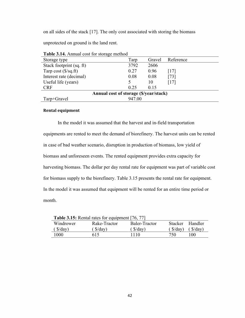
42

on all sides of the stack [17]. The only cost associated with storing the biomass

unprotected on ground is the land rent.

Table 3.14. Annual cost for storage method Storage type Tarp Gravel Reference Stack footprint (sq. ft) 3792 2606 Tarp cost ($/sq.ft) 0.27 0.96 [17] Interest rate (decimal) 0.08 0.08 [73] Useful life (years) 5 10 [17] CRF 0.25 0.15

Annual cost of storage ($/year/stack) Tarp+Gravel 947.00 Rental equipment

In the model it was assumed that the harvest and in-field transportation

equipments are rented to meet the demand of biorefinery. The harvest units can be rented

in case of bad weather scenario, disruption in production of biomass, low yield of

biomass and unforeseen events. The rented equipment provides extra capacity for

harvesting biomass. The dollar per day rental rate for equipment was part of variable cost

for biomass supply to the biorefinery. Table 3.15 presents the rental rate for equipment.

In the model it was assumed that equipment will be rented for an entire time period or

month.

Table 3.15: Rental rates for equipment [76, 77] Windrower ( $/day)

Rake-Tractor ( $/day)

Baler-Tractor ( $/day)

Stacker ( $/day)

Handler ( $/day)

1000 615 1110 750 100

43

Case study assumptions and inputs for the model Table 3.16. List of inputs for the case study (base scenario) Description Value Ref. Biomass type Switchgrass Biorefinery location Hugoton , Kansas Biorefinery demand 800 dry tons/day [78] Yield of biomass Base scenario: 2 dry tons/acre [79, 80] Biomass supply counties Grant (KS), Haskell (KS), Morton (KS),

Seward (KS), Stanton (KS), Stevens (KS), Texas (OK)

[81]

Biomass cost $18.50 per ton [63] Land categories considered Non-irrigated cropland

Permanent pasture Expired- CRP

[82, 83]

Proportion of each land category for biomass production

Non-irrigated cropland: 25% Permanent pasture: 50% Expired- CRP: 50%

[54, 82, 84]

Land rent for each land category Non-irrigated cropland: $60/acre Permanent pasture: $40/acre Expired- CRP: $55/acre

[54, 56, 85]

Total acres of land considered for biomass production

Non-irrigated cropland: 913,545 acre Permanent pasture: 904,866 acre Expired- CRP: 135,723 acre

[86, 87]

Harvest unit Self-propelled windrower, rake-tractor, large square baler-tractor

In-field transportation unit Stacker, bale handler Transportation unit Semi-trailer truck Weather data Daily weather data from Oklahoma Mesonet [1] Number of years of weather data considered

12

Probability of weather scenario 0.0831 Storage treatments Tarp + Gravel,

Untarped + Ground [88]

Storage treatment dry matter loss Tarp + Gravel: 0.33% Untarped + Ground : 0.33%

[88]

Cost of biomass from outside source $90/ton (50% higher the delivered cost of biomass $60/ton considered by U.S. Billion ton update [89])

Cost of selling excess biomass to feedlot

25% of dollar per ton cost of biomass ($4.56/ton)

The case study was developed for the Abengoa Biorefinery (AB) at Hugoton, KS

(Figure 3.2). AB considers switchgrass to be a potential biofeedstock. Twelve weather

scenarios from 1998-2010 were considered. The reason for selecting these weather

44

scenarios was that the Oklahoma Mesonet started measuring the FWI values from 1998.

These values were needed for calculating soil moisture content and eventually the

number of harvest workdays. Equal probability of occurrence of 0.0831(1÷12) was

assigned to each of the twelve weather scenarios. The 50 mile radius was defined as the

feedstock procurement area [34] which includes Morton, Stanton, Grant, Haskell,

Seward, and Stevens counties in KS and Texas County in OK [34] (Table 3.17 & Figure

3.3). Also, switchgrass has a wide harvest window of eight months starting from July to

February [90] which results in only four months of non-harvesting season. A one-year

planning period with monthly time increments was considered.

Table 3.17. Switchgrass source counties considered for the case study Texas (OK)

Morton (KS)

Stanton (KS)

Stevens (KS)

Grant (KS)

Haskell (KS)

Seward (KS)

So-1 So-2 So-3 So-4 So-5 So-6 So-7

Figure 3.2. Abengoa biorefinery (AB) site at Hugoton, Kansas

45

Figure 3.3. A 50-mile area of influence around Abengoa Biorefinery (AB) at

Hugoton, Kansas

For the operation of the biorefinery, two alternatives are proposed by AB: the

proposed action and the action alternatives with demand of 2500 and 800 dry tons per

day, respectively. The daily demand of 800 dry tons of switchgrass was considered for

the present case study with a nominal production schedule of 350 days per year [34].

Since switchgrass is not commercially available in the feedstock procurement area of

influence, an assumption was made that the farmers would convert their land to

switchgrass production. The Billion-Ton Update-2011[82] considered non-irrigated

harvested cropland and permanent pasture as land categories for the production of energy

crops. The study also mentioned marginal lands such as land enrolled in CRP program as

a potential producer of bioenergy crops. The land enrolled under the Conservation

Reserve Program (CRP) could be available for AB. CRP is a voluntary program for the

agricultural landowners receiving annual rental payments for their land. The acres

enrolled under CRP are to protect wildlife, reduce soil erosion, and conserve vegetative

46

cover [91]. AB anticipates that the expired CRP land will not be re-enrolled and contracts

for CRP land will not be extended in the CRP program [34]. For the present study, it was

assumed that non-irrigated harvested cropland, permanent pasture, and expiring and not

re-enrolled CRP acres in the year 2011 and 2012 will be used for switchgrass production.

Table 3.18 presents the acres by county in each land considered for the production of

switchgrass. The proportion of cropland and pastureland used considered for switchgrass

production was adapted from the billion-ton update report [89] (Table 3.16). It was also

assumed that up to 50% of CRP land can be used for switchgrass production [54, 84].

Table 3.18. Acres by county and land category in Kansas and Oklahoma [86] County (State) Non-irrigated

harvested cropland Permanent pasture

Total expired CRP acres

Grant (KS) 88533 54320 7122 Haskell (KS) 86520 61835 5738 Morton (KS) 178875 61056 6839 Seward (KS) 75324 94291 8083 Stanton (KS) 204776 40342 36764 Stevens (KS) 101724 89851 25537 Texas (OK) 177793 503171 45642

Switchgrass reaches its full yield potential in the third year of its planting [92].

The yield of switchgrass varies for each county and depends on soil type, precipitation,

fertility, cultivar, and other agronomic/climatic growing conditions [93]. Yield decreases

with maturity and the model assumes a yield loss factor of 5% per month from September

through February [94]. The AB anticipates an average yield of 1.5-3.0 dry tons per acre

for switchgrass from the soil types and climatic patterns present in the region [34, 95].

Lee et al. [79] found that the maximum yield of mixture of warm season perennial

grasses planted on CRP acres in North Dakota, Kansas, and Oklahoma ranged from 1.71-

47

3.21 tons per acre. In the present study, the yield of switchgrass was assumed to be 2 dry

tons per acre.

For the model demonstration, five inventory sites were selected based on road

accessibility and the distance from the biorefinery of about 30 miles [34]. AB plans to

have five to seven inventory sites [81]. ArcGIS 10 software [2] was used for selection of

the inventory sites. The data for the county, road, populated, and unpopulated areas were

extracted from Geospatial Data Gateway in shape file format [97]. The raster file for the

cropland data layer was extracted from the USDA, National Agricultural Statistics

Service [98].The data was collected for Morton, Stanton, Grant, Haskell, Seward and

Stevens counties in KS and Texas County in OK. The proximity to a road network is

highly desirable as it helps to decrease the transportation cost and the overall production

price of bioethanol. A distance between 650 ft. and 6,500 ft. from a road network was

considered for site selection. The distance less than 650 ft. was not suitable due to

aesthetic consideration [99]. The distance greater than 6,500 ft. from a road network was

not considered due to the expected increase in the transportation cost [99]. A buffer layer

of 650 ft. and 6,500 ft. was created around the road network and another buffer layer of

25 to 30 miles was created around the biorefinery site using ArcGIS. The buffer layers

created are shown in Figure 3.4. Out of the potential sites, the sites having areas equal to

the desired inventory site area were selected. Of the five inventory sites selected, four

inventory sites were off-site storage sites, and the fifth inventory site at Stevens County

was an on-site storage site in the biorefinery (Table 3.19). Eight hundred acres were

allocated to all inventory sites. These acres would provide enough capacity for biomass

storage to support biorefinery operation for up to two years. For the present model, it was

48

assumed that safety stock of biomass at inventory sites would be enough to support

biorefinery operation for up to one year. The ending inventory was assumed to be equal

to beginning inventory. The extra storage capacity will accommodate seasonality of

production and uncertainty in weather to ensure regular supply to the biomass to the

biorefinery.

The storage capacity was enough to meet up to one year demand of the

biorefinery as required by AB [81]. The distances between the sites were calculated using

the great circle distance formula. The distances between the biomass source sites,

inventory sites, and biorefinery site, and their associated variable cost of transportation is

presented in Table 3.20 and Table 3.21. The monthly dry matter loss during storage is

presented in Table 3.22. The dry matter loss values were obtained from experiment

conducted at Panhandle Oklahoma for storing square switchgrass bales. The reason for

same dry matter loss values was attributed to extremely dry weather conditions during the

storage period.

49

Figure 3.4. The buffer layer for road network and distance from biorefinery site for

determining potential inventory sites

Table 3.19. Location of inventory sites County Notation Latitude Longitude Address Seward, KS Inv-1 37.215 -100.860 Kismet, KS 67859 Grant, KS Inv-2 37.576 -101.324 2001-2501 Hampton Ave, Ulysses, KS 67880 Morton, KS Inv-3 37.125 -101.887 Cimarron National Grassland, Elkhart, KS 67950 Texas, OK Inv-4 36.793 -101.316 N0950 Rd, Hooker, OK 73945 Stevens, KS Inv-5 37.179 -101.386 Road P, Hugoton, KS, 67951 Table 3.20. Distance and variable cost from inventory site to biorefinery site, and biomass source site to biorefinery site *Inv-1 *Inv-2 *Inv-3 *Inv-4 *Inv-5 Round trip distance (miles) 62.72 56.38 59.89 52.51 1.44 Total variable cost ($/ton) 6.0 5.5 5.8 5.2 1.5 *So-1 *So-2 *So-3 *So-4 *So-5 *So-6 *So-7 Round trip distance (miles) 92.89 70.94 91.20 11.46 81.33 93.58 91.32 Total variable cost ($/ton) 8.2 6.6 8.1 2.2 7.3 8.2 8.1 *For name of Inv# sites and So# sites refer to Table 3.18 and Table 3.20

50

Table 3.21. Distance and variable cost from source site to inventory site Round trip distance (miles) Variable cost ($/ton) *So-1 *So-2 *So-3 *So-4 *So-5 *So-6 *So-7 *So-1 *So-2 *So-3 *So-4 *So-5 *So-6 *So-7

Inv-1 122 133 152 80 79 54 22 10.3 12.5 7.7 4.3 8.3 10.3 12.5 Inv-2 152 118 86 58 30 68 108 11.1 10.0 2.8 6.5 6.6 11.1 10.0 Inv-3 86 19 62 62 132 154 152 12.5 7.7 5.9 11.0 7.9 12.5 7.7 Inv-4 41 70 132 68 132 129 95 7.2 5.6 5.9 6.4 2.1 7.2 5.6 Inv-5 94 71 90 10 81 94 92 7.2 3.6 11.0 11.0 7.3 7.2 3.6

*For Inv# sites and So# sites notations are described Table 3.17 and Table 3.15

Table 3.22. Monthly storage dry matter loss in each storage treatment [32, 100] Storage treatment Notation Dry matter loss (%) Gravel + Tarp GT 0.33 Unprotected UP 0.33

Switchgrass can be harvested before frost and after frost [101]. The moisture

content of switchgrass after frost decreases to a safe baling moisture content. The low

moisture content facilitates windrowing without conditioning, baling without raking, easy

handling, storage, and size reduction. By delaying harvest until after the first hard frost

period, translocation of nutrients such as nitrogen, phosphorous and potassium takes

place. This translocation of nutrients form mature switchgrass shoots to roots and

decreases the need for fertilization in subsequent years [9, 102]. In addition, the

translocation of nutrients may decrease the tonnage, but increase the carbon percentage

which in turn might improve the conversion efficiency and combustion quality. The

disadvantage with harvest after frost is that the grass is brittle due to low moisture content

and shattering losses of leaves and stems may occur. Before and after frost harvesting of

switchgrass was considered in the model. The freeze in Oklahoma usually begins in late

October to early November [103]. A Matlab program [104] was developed to determine

the time periods before frost and after frost. A day was considered to be before frost if the

minimum temperature was above 32oF. If 60% of the days in a month met the criteria,

the month was considered to be “before frost” for classification purposes. Table 3.23

51

shows before and after frost time periods for all weather scenarios considered in the

model. The results show that the frost usually begins in the month of November in

Oklahoma. The results are consistent with those found by Koss et al. [103].

Table 3.23. The time periods before and after frost in each weather scenario (1 indicate before frost and 0 indicate after frost) derived from weather data and processed in Matlab Month Notation WS-1 WS-2 WS-3 WS-4 WS-5 WS-6 WS-7 WS-8 WS-9 WS-10 WS-11 WS-12 July TP-1 1 1 1 1 1 1 1 1 1 1 1 1 Aug TP-2 1 1 1 1 1 1 1 1 1 1 1 1 Sep. TP-3 1 1 1 1 1 1 1 1 1 1 1 1 Oct. TP-4 1 1 1 1 1 1 1 1 1 1 1 1 Nov TP-5 1 1 0 1 0 0 0 0 0 0 0 0 Dec. TP-6 0 0 0 0 0 0 0 0 0 0 0 0 Jan. TP-7 0 0 0 0 0 0 0 0 0 0 0 0 Feb. TP-8 0 0 0 0 0 0 0 0 0 0 0 0

WS= Weather Scenario, TP=Time Period

Model description

The model equations with definition of decision variables, parameters, and

formulation are described in Appendix-B. The objective function of the model was to

minimize cost of biomass supply to the biorefinery.

Decision variables

The following decision variables are included in the model:

• The acres leased for switchgrass production in a source county and land category

• The quantity of biomass harvested from each biomass source site under each

weather scenario and time period

• The quantity of biomass transported from the biomass source site to the

biorefinery site and inventory sites under each weather scenario and time period

• The quantity of biomass transported from each inventory site to the biorefinery

site in each weather scenario and time period

52

• The number of harvest unit, in-field transportation unit, and transportation unit

required to be purchased and deployed under all-weather scenarios

• The number of harvest units, in-field transportation units, and transportation units

required to be rented and deployed under all-weather scenarios

• The storage treatment used for storing biomass at the inventory sites and the

number of storage units required under all-weather scenarios

• The quantity of biomass purchased from outside source to meet the demand of

biorefinery

• The quantity of biomass sold if excess biomass is produced

Model constraints

Supply constraints: These constraints consider the biomass harvested quantity of

biomass available, biomass transported for each weather scenario and time period. The

total acres of biomass harvested must not exceed the total acres contracted for biomass

cultivation in each biomass source site, weather scenario, and time period. The supply

constraints also consider the total tonnage procured by the biorefinery which is equal to

the acres of biomass harvested multiplied by the yield and yield adjustment factor. The

yield adjustment factor varies between 0 and 1 and adjusts the change in yield of biomass

with the harvest time periods.

The storage of biomass at the harvesting sites or biomass source sites was not

considered as it is assumed that farmers will not be willing to allocate their land for

storing biomass. The biomass source sites were not considered for storing biomass;

therefore, the total biomass harvested at the source site is equal to the biomass

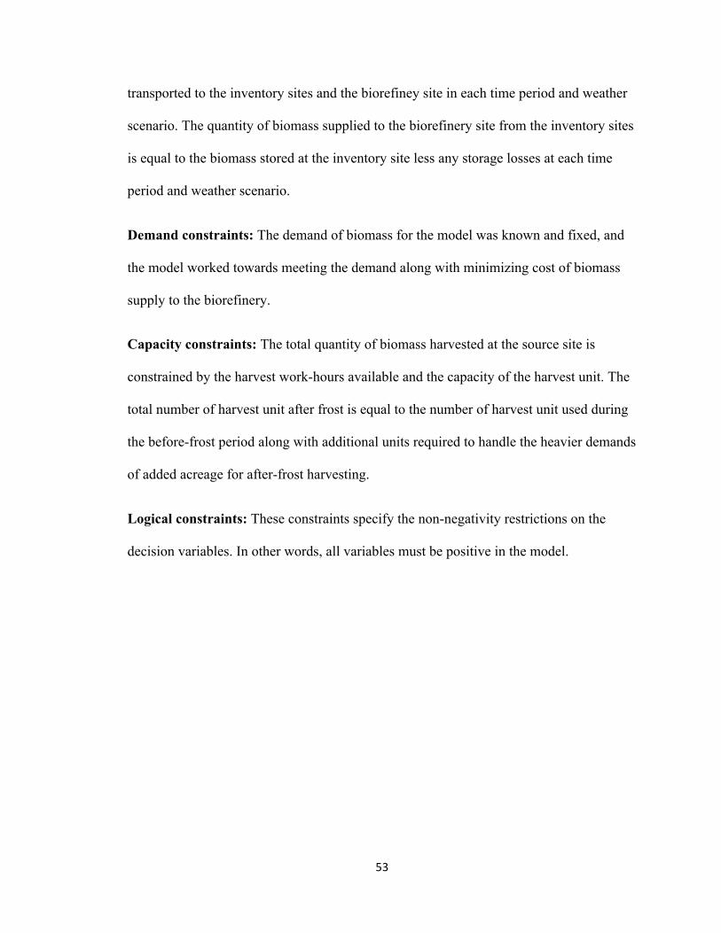
53

transported to the inventory sites and the biorefiney site in each time period and weather

scenario. The quantity of biomass supplied to the biorefinery site from the inventory sites

is equal to the biomass stored at the inventory site less any storage losses at each time

period and weather scenario.

Demand constraints: The demand of biomass for the model was known and fixed, and

the model worked towards meeting the demand along with minimizing cost of biomass

supply to the biorefinery.

Capacity constraints: The total quantity of biomass harvested at the source site is

constrained by the harvest work-hours available and the capacity of the harvest unit. The

total number of harvest unit after frost is equal to the number of harvest unit used during

the before-frost period along with additional units required to handle the heavier demands

of added acreage for after-frost harvesting.

Logical constraints: These constraints specify the non-negativity restrictions on the

decision variables. In other words, all variables must be positive in the model.

54

References [1] Mesonet. Past data and files; c1994-2012 [cited 2012 24 Aug]. Available from:

http://www.mesonet.org/. [2] ESRI. ArcGIS 10.1. 2011. [3] Tembo G, Epplin FM, Huhnke RL. Integrative investment appraisal of a

lignocellulosic biomass-to-ethanol industry. J Agr Resour Econ. 2003;28(3):611-633.

[4] Sorensen C. Workability and machinery sizing for combine harvesting. Agricultural Engineering International: the CIGR Journal of Scientific Research and Development. 2003;V:1-19.

[5] Christensen CA, Koppenjan G. Planting and managing switchgrass as a dedicated energy crops. Blade Energy Crops, 2010.

[6] Herron M. Throughput of harvest equipment. B. Sharma. 3 October 2012 2012. [7] Sokhansanj S, Turhollow A, Wilkerson E. Development of the integrated biomass

supply analysis and logistics model (IBSAL) Oak Ridge National Laboratory, Oak Ridge, Tennessee;2008 37831-6283.

[8] ASABE. EP496.3. Agricultural machinery management 2006. [9] Thorsell S, Epplin FM, Huhnke RL, Taliaferro CM. Economics of a coordinated

biorefinery feedstock harvest system: lignocellulosic biomass harvest cost. Biomass Bioenergy. 2004;27(4):327-337.

[10] Popp M, Hogan JR. Assessment of two alternative switchgrass harvest and transport methods. Farm Foundation Conference, Louis, Missouri, 2007. p. 9.

[11] Larson JA, Yu TH, English BC, Mooney DF, Wang C. Cost evaluation of alternative switchgrass producing, harvesting, storing, and transporting systems and their logistics in the Southeastern USA. Agricultural Finance Review. 2010;70(2):184-200.

[12] Hanna M. Estimating the field capacity of farm machines. 1-4. Available from: http://www.extension.iastate.edu/agdm/crops/pdf/a3-24.pdf;2002.

[13] Srivastava AK, Carroll GE, Roger RP, Dennis BR. Machinery selection and management., in Engineering Principles of Agricultural Machines, 2 ed Michigan: ASABE. , 2006, pp. 525-552.

[14] ASABE. D497.5: Agricultural machinery management data. . 2006. [15] Kemmerer B, Liu J. Large square baling and bale handling efficiency—A case

study. Agricultural Sciences. 2012;3(2):178-183. [16] ASABE. Standards. ASAE EP496.3 FEB2006, Agricultural machinery

management. 2006. [17] Turhollow A, Wilkerson E, Sokhansanj S. Cost methodology for biomass

feedstocks: Herbaceous crops and Agricultural residues. Oak Ridge Natinal Laboratory, US Department of Energy, 2009.

[18] Stinger stacker 6500. c2009 [cited 2011 Jul 30]. Available from: http://www.stingerltd.com/stinger.htm.

[19] Blubaugh V. Stinger Inc. 2012. [20] Dymax. Hay squeeze; c2011 [cited 2011 Dec 25 ]. Available from:

http://www.dymaxinc.com/attachments/6051/. [21] Larson ED, Fiorese G, Liu G, Williams RH, Kreutz TG, Consonni S. Co-

production of decarbonized synfuels and electricity from coal + biomass with

55

CO2 capture and storage: an Illinois case study. Energy & Environmental Science. 2010;3(1):28-42.

[22] Sokhansanj S, Turhollow AF. Baseline cost for corn stover collection. Applied Engineering in Agriculture. 2002;18(5):525–530.

[23] Berwick M, Dooley F. Truck costs for owner/operators. North Dakota State University, Fargo;1997.

[24] Wideberg J, Dahlberg E, Svensson M. Study of stability measures and legislation of heavy articulated vehicles in different OECD countries; c2006 [cited 2011 Aug 13 ]. Available from: www.mne.psu.edu/ifrtt/ConferenceProceedings/ISHVWD_9_2006/docs/pdfs/session%206/s6-2%2090.pdf.

[25] DPS. Size, weight and load; c2011 [cited 2011 Dec 27]. Available from: http://www.dps.state.ok.us/ohp/chapter14.pdf.

[26] Tolliver D, Berwick M, Vachal K. Farm-to-market transportation patterns and truck use in the Northern Plains. Upper Great Plains Transportation Institute;2005.

[27] Keramati A, Eldabi T. Supply chain integration: Modelling approach presented at the European, Mediterranean & Middle Eastern Conference on Information Systems, Athens, Greece, 2011.

[28] Simchi-Levi D, Kaminsky P, Simchi-Levi E. Designing and managing the supply chain: concepts, strategies and case studies, 3 ed.: McGraw-Hill Education, 2008.

[29] Simchi-Levi D, Kaminsky P, Simchi-Levi E. Designing and managing the supply chain: concepts, strategies, and case studies. New York: The McGraw-Hill Companies, Inc., 2003.

[30] Hess JR, Kenney KL, Wright CT, Perlack R, Turhollow A. Corn stover availability for biomass conversion: situation analysis. Cellulose 2009;16:599–619.

[31] Miranowski J. Economics of feedstock production, harvest, storage, and transport. Proceedings of the sustainable feedstocks for advance biofuels workshop, Atlanta, GA 2010. pp. 177-192.

[32] Khanchi A. Drying and storage of switchgrass [Dissertation]. Biosystems and Agricultural Engineering, Oklahoma State University, Stillwater; 2012.

[33] ICC. International fire code 2903.4. International Code Council, Inc, I. C. Council, Ed., ed, 2003.

[34] DOE/EIS. Final environmental impact statement for the proposed Abengoa Biorefinery Project near Hugoton, Stevens County, Kansas. Golden Field Office, Office of Energy Efficiency and Renewable Energy 2010. DOE/EIS-0407.

[35] Mapemba LD. Cost to deliver lignocellulosic biomass to a biorefinery [Dissertation]. Oklahoma State University, 2005.

[36] Baier W. Estimation of field work-days in Canada from the versatile soil moisture budget. Can. Agric. Eng. 1973;15(2):84-87.

[37] Donaldson GF. Allowing for weather risk in assessing harvest machinery capacity. American Journal of Agricultural Economics. 1968;50(1):24-40.

[38] Rounsevell MDA, Jones RJA. A soil and agroclimatic model for estimating machinery work-days: the basic model and climatic sensitivity. Soil and Tillage Research. 1993;26(3):179-191.

56

[39] Earl R. Prediction of trafficability and workability from soil moisture deficit. Soil and Tillage Research. 1997;40(3-4):155-168.

[40] Simalenga TE, Have H. Estimation of soil tillage workdays in a semi-arid area. Journal of Agricultural Engineering Research. 1992;51:81-89.

[41] Hoogenboom G, Jones JW, Wilkens PW, Porter CH, Boote KJ, Hunt LA, et al. Decision Support System for Agrotechnology Transfer (DSSAT) Version 4.5 [CD-ROM]. 2010.

[42] NOAA. Most Requested H: Integrated Surface Hourly; c2010 [cited 2010 August 25]. Available from: http://www.noaa.gov/index.html.

[43] Sandor D, Wallace R, Peterson S. Understanding the growth of the cellulosic ethanol industry. National Renewable Energy Laboratory, Colorado;2008.

[44] Bergman PCA. Combined torrefaction and pelletisation: The TOP process. Energy Research Center of the Netherlands (ECN), The Netherlands;2005.

[45] Allen RG, Pereira LS, Raes D, Smith M. Crop evapotranspiration - Guidelines for computing crop water requirements - FAO Irrigation and drainage paper 56. FAO - Food and Agriculture Organization of the United Nations, Rome. 1998 paper no. 56 1-281.

[46] Hwang S. Days available for harvesting switchgrass and the cost to deliver switchgrass to a biorefinery Agricultural Economics, Okalahoma State University, Stillwater; 2007.

[47] Instruments. c1994 [cited 2012 1 February]. Available from: http://www.mesonet.org/index.php/site/about/moisture_measurements.

[48] Hwang S, Epplin FM, Lee B-h, Huhnke R. A probabilistic estimate of the frequency of mowing and baling days available in Oklahoma USA for the harvest of switchgrass for use in biorefineries. Biomass and Bioenergy. 2009;33(8):1037-1045.

[49] Uslu A, Faaij APC, Bergman PCA. Pre-treatment technologiees, and their effect on international bioenergy supply chain logistics. Techno-economic evaluation of torrefaction fast pyrolysis and pelletisation. Energy. 2008;33:1206-1223.

[50] Mesonet. Fractional Water Index; c2011 [cited 2011 Dec 25 ]. Available from: http://www.mesonet.org/.

[51] Reinschmiedt LL. Study of the relationship between rainfall and fieldwork time available and its effect on optical machinery selection Agricultural Economics, Oklahoma State University, Stillwater; 1973.

[52] W J, Helm JL, Brenk PC. Potential field work days during planting and harvesting c1995 [cited 2011 Aug 25]. Available from: http://www.ag.ndsu.edu/pubs/plantsci/crops/a1008w.htm.

[53] daylightHoursExplorer008. Daylight Hours Explorer. 2010. [54] Fewell J, Bergtold J. Farmer's willingness to grow switchgrass as a cellulosic

bioenergy crop: A stated choice approach. Annual Meeting of the Canadian Agricultural Economics Society & Western Agricultural Economics Association Banff, Alberta, Canada, 2011.

[55] Haque M. Switchgrass biomass to ethanol production economics: field to fuel approach. Agricultural Economics, Oklahoma State University, Stillwater, Oklahoma; 2010.

57

[56] Mohua H, M EF. Cost to produce switchgrass and cost to produce ethanol from switchgrass for several levels of biorefinery investment cost and biomass to ethanol conversion rates. Biomass and Bioenergy. 2012;46:517-530.

[57] Huhnke RL, Venkateswaran AK, Basina V. AGMACH$:Agricultural Field Machinery Cost Estimator. 2008.

[58] USDA. Machinery cost estimates: Summary 2010. [59] Massey-Ferguson 2170. c2011 [cited 2011 Aug 25]. Available from:

http://www.tractorhouse.com/list/list.aspx?Pref=1&ETID=1&Mdltxt=2170&Manu=MASSEY-FERGUSON&mdlx=contains&bcatid=464.

[60] Build and price your own Case IH equipment. c2011 [cited 2011 Aug 25]. Available from: http://caseih.ironbuilder.com/Series/Hay_(_and_)_Forage.aspx.

[61] KRONE Configurator. c2011 [cited 2011 Aug 25]. Available from: http://www.krone-northamerica.com/english/products/krone-configurator/.

[62] Built and Price your New Holland. c2011 [cited 2011 Jul 30 ]. Available from: http://nh.ironbuilder.com/default.aspx.

[63] EERE. Biomass multi-year program plan. U.S. Department of Energy 2011. [64] Bakht GMK, Ahmadi H, Akram A, Karimi M. Repair and maintenance cost

models for MF285 tractor: A case study in central region of Iran. American-Eurasian J. Agric. & Environ. Sci. 2008;4(1):76-80.

[65] USDA-NASS. 2007 Census of Agriculture -Oklahoma, County Data, USDA, Ed., ed. Washington, DC: United State Department of Agriculture, National Agriculture Statistics Service, 2007.

[66] Kastens T. Farm machinery operation cost calculations. 1997. [67] cost Etf. c2011 [cited 2010 Aug 24]. Available from:

http://www.uwagec.org/farmmgt/Software/Impact-tractorfuell.xls [68] Jacobs J, Mount D, Freeburn J. Impact of Fuel Prices on Per-Acre Costs 2005. [69] BLS. Truck drivers and driver/sales workers; c2010 [cited 2012 Feb 13].

Available from: http://www.bls.gov/oco/ocos246.htm. [70] Svetgoff JW. Developing a budget to plant, harvest and transport switchgrass [ ].

Agricultural Economics, Oklahoma State University, Stillwater; 2009 [71] EIA. Gasoline and diesel fuel Update; c2012 [cited 2012 Feb 13]. Available from:

http://www.eia.gov/petroleum/gasdiesel/. [72] Company KT. Kenworth truck company white paper on fuel economy; c2008

[cited 2012 Feb 13]. Available from: http://www.kenworth.com/1000_hom.asp. [73] USDA. Chariton valley biomass project. Chariton Valley RC&D;2002. [74] Huisman W, Jenkins B, Summers M. Storage systems for rice straw in California.

University of California, Davis, 2005. [75] M.D.Duffy, Nanhou VY. Costs of producing switchgrass for biomass in Southern

Iowa. 2001. [76] SwiderskiEquipment. Agriculture equipment: Rental rates; c2012 [cited 2012 26

Dec]. Available from: http://www.swiderskiequipment.com/rental_rates.php. [77] DeBlaey J. 2012 Equipment Rentals; c2012 [cited 2012 26 Dec]. Available from:

http://www.gibbsvilleimplement.com/pdf/2012rental.pdf. [78] DOE. Final enviornmental impact statement for the Abengoa Biorefinery Project

near Hugoton, Stevens County, Kansas: Introduction and purpose and need. 2010. DOE/EIS-0407.

58

[79] Lee D, Aberle E, Chen C, Egenolf J, Harmoney K, Kakani G, et al. Nitrogen and harvest management of Conservation Reserve Program (CRP) grassland for sustainable biomass feedstock production. GCB Bioenergy. 2012:1-10.

[80] Huhnke R, Jones CL. Yield of switchgrass in panhandle, oklahoma. B. Sharma. 16 October 2012 2012.

[81] DOE. Final enviornmental impact statement for the Abengoa biorefinery project near Hugoton, Stevens County, Kansas: Affected environment. 2010. DOE/EIS-0407.

[82] Perlack RD, 2011 BJS. U.S. Billion-ton update: Biomass supply for a bioenergy and bioproducts industry. Oak Ridge National Laboratory and U.S. Department of Energy, Oak Ridge, TN;2011.

[83] Huhnke R, Jones CL. Land category for biomass cultivation. B. Sharma. 13 August 2012 2012.

[84] Khanna M, Chen X, Huang H, Onal H. Supply of cellulosic biofuel feedstocks and regional production patterns. Journal of Agricultural Economics. 2011:1-8.

[85] Epplin FM. Rental rate for cropland, patureland and CRP acres used for biomass production. B. Sharma. 30 Aug 2012.

[86] USDA-FSA. CRP Contract expirations by County, 2011-2017; c2011 [cited 2011 Jul 26]. Available from: http://www.fsa.usda.gov/FSA/webapp?area=home&subject=rsch&topic=css.

[87] USDA-NASS. Cencus of Agriculture: Kansas State and County Data United State Department of Agriculture, National Agriculture Statistics Service;2007. 16.

[88] Miller E. Dry matter loss in large switchgrass square bales stored in Panhandle, Oklahoma. B. Sharma. 2012.

[89] Perlack RD, Stokes BJ. U.S. Billion-ton update: Biomass supply for a bioenergy and bioproducts industry. Oak Ridge National Laboratory, 2011.

[90] Epplin FM. Cost to produce and deliver switchgrass biomass to an ethanol-conversion facility in the southern plains of the United States. Biomass and Bioenergy. 1996;11(6):459-467.

[91] USDA-FSA. Conservation Reserve Program (CRP); c2010 [cited 2011 Jan 18 ]. Available from: http://www.apfo.usda.gov/FSA/webapp?area=home&subject=copr&topic=crp.

[92] Myhre MA. Farm net income impact of switchgrass production and corn collection for heat and power generation Gaylord Nelson Institute for Environmental Studies, University Of Wisconsin, Madison; 2010.

[93] Nelson R. Cellulosic ethanol / bioethanol in Kansas Kansas Energy Council Biomass Committee 2007. 15 May 2007.

[94] Epplin FM, Clark CD, Roberts RK, Hwang S. Challenges to the development of a dedicated energy crop. American Journal of Agricultural Economics 2007;89(5):1296-1302.

[95] USDA. BCAP project area applications. 2011. [96] Bevill K. Abengoa offers details on biomass supply agreement, in Ethanol

producer Magazine, ed, 2011. [97] Gateway GD. United States Department of Agriculture, Natural Resource

Conservation Service, Geospacial Data Gateway; c2011 [cited 2011 Dec 24]. Available from: http://datagateway.nrcs.usda.gov/.

59

[98] USDA-NASS-RDD. Cropland data layer; c2011 [cited 2011 Dec 24]. Available from: http://www.nass.usda.gov/research/Cropland/SARS1a.htm.

[99] Brunskill D, Lung I, Murad G. A GIS approach for siting a bio-ethanol plant within Chouteau County, Montana. 2011.

[100] Miller E. Dry matter loss in large square bales stored in Panhandle, Oklahoma. B. Sharma. Oct 22 2012.

[101] Garland CD. Growing and harvesting switchgrass for ethanol production in Tennessee; c2008 [cited 2011 July 28 ]. Available from: https://utextension.tennessee.edu/publications/Documents/SP701-A.pdf.

[102] Sharma B, Jones CL, Khanchi A. Tensile strength and shear strength of switchgrass before and after frost. Biological Engineering Transactions. 2011 4(1):43-54.

[103] Koss WJ, Owenby JR, Steurer PM, Ezell DS. Freeze and frost data. National Oceanic and Atmospheric Administration, U.S. Department of Commerce;1998.

[104] MathWorks. Matlab & Simulink. 2009.

60

CHAPTER IV

RESULTS AND DISCUSSION

61

The scenario optimization model was developed to minimize cost of the biomass

supply to the biorefinery. The model determines the system cost, material flow, and

number of machinery units purchased or rented. The model facilitates strategic,

operational and tactical planning for a biorefinery. The strategic decisions are based on

minimizing the fixed and variable costs of machinery, labor, management, investment,

and operation. The tactical and operational decisions account for only variable cost and

work towards improving the profitability of managing day-to-day decisions [1]. The

optimization model was solved using Xpress-IVE version 1.22.04 tool (Fair Isaac

Corporation (FICO®2001-2012).

The model was first evaluated for the base scenario. The base scenario run for the

model consists of all inputs to the model assumed for the Abengoa Biorefinery (AB)

presented in Table 3.16 and cost inputs presented in Table 3.11, 3.12, 3.14, 3.15, 3.20 and

3.21.

Sensitivity analysis is a technique to evaluate the impact of certain inputs on the

model results, by keeping all other inputs at same value, as for the base scenario. It is a

way to predict the change in outcome of the model with an unexpected deviation in the

situation. Different scenarios can be evaluated for the critical inputs of the model which

help analysts to determine the possible outcomes under those scenarios. For the present

study, sensitivity analysis was done on yield, storage dry matter loss, and land rent.

The results section is organized by first presenting the results for determining harvest

works hours in different weather scenarios. Next, the results for the base scenario run of

the model for AB are presented. Then the sensitivity analysis results are discussed with

conclusion at the end the end of the chapter.

62

Harvest work hours

The weather patterns during each weather scenario determined the number of

suitable work hours for harvesting switchgrass in a certain time period. The actual

weather conditions cannot be predicted in advance; therefore, the decisions about the

purchase of the machinery were made based on the past weather data. This might result in

excess machinery capacity during some years and insufficient machinery capacity during

other years. To deal with this situation, weather data for several years should be used for

analysis. In the present study, twelve years of weather data was considered beginning

from 1997 to 2010 with each year considered as different weather scenario (Appendix-C,

Table C-1). As more weather data is collected, more accurate predications can be

included. Figure 4.1 represents the work hours available for harvesting switchgrass in

each weather scenario and time period. It was assumed that 80% daylight hours were

used for harvesting switchgrass. Twenty percent of the daylight hours were assumed to be

lost due to the machinery breakdown, unavailability of labor, and unforeseen events. The

average monthly harvest work hours available in each weather scenario were found to be

statistically (P=0.0004) different. A harvest time period was considered from July to

February. It was observed that the average work hours available for harvesting

switchgrass for all harvest time periods varied from a minimum of 185 hours to the

maximum of 237 hours in 1999-2000 and 2009-2010 weather scenario, respectively. The

harvesting units were purchased/rented and deployed to the switchgrass source sites by

the biorefinery. Therefore, it was assumed that the harvesting operation will be done on a

rigid schedule utilizing maximum harvest hours available to minimize the cost of the

biomass supply to the biorefinery.

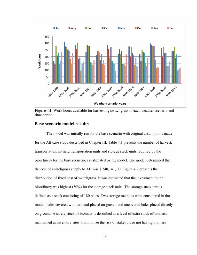
63

Figure 4.1. Work hours available for harvesting switchgrass in each weather scenario and time period Base scenario model results The model was initially run for the base scenario with original assumptions made

for the AB case study described in Chapter III. Table 4.1 presents the number of harvest,

transportation, in-field transportation units and storage stack units required by the

biorefinery for the base scenario, as estimated by the model. The model determined that

the cost of switchgrass supply to AB was $ 240,141, 00. Figure 4.2 presents the

distribution of fixed cost of switchgrass. It was estimated that the investment to the

biorefinery was highest (50%) for the storage stack units. The storage stack unit is

defined as a stack consisting of 180 bales. Two storage methods were considered in the

model: bales covered with tarp and placed on gravel; and uncovered bales placed directly

on ground. A safety stock of biomass is described as a level of extra stock of biomass

maintained at inventory sites to minimize the risk of stakeouts or not having biomass

0

50

100

150

200

250

300

350 Workh

ours

Weather scenario, years

Jul Aug Sep Oct Nov Dec Jan Feb

64

available to meet the biorefinery requirement. In the present model, it was assumed that a

safety stock of a one- year switchgrass supply was stored at the inventory sites with bales

covered with tarp and placed on gravel. The safety stock of switchgrass maintained at the

inventory sites added a significant cost to the overall cost of biomass supply to the

biorefinery.

The factors considered for making decisions on purchasing equipment are harvest

work hours, yield of biomass, and cost of purchasing machinery and renting machinery.

Yu et al. [2] found that it is more economical for the biorefinery or biomass growers to

purchase and coordinate equipment as opposed to contracting independent third-party

service providers. For this study, it was assumed that AB will be responsible for

purchasing or renting the equipments for receiving biomass to the biorefinery gate.

Twenty three transportation units account for 28% of the total cost of investment in

purchasing units by the biorefinery. The harvest unit cost account for 17% of the total

investment cost with five harvest units purchased by the biorefinery. In the base scenario,

the yield of switchgrass was assumed to be 2 dry tons per acre. At low yields of biomass,

rake operation is required throughout the harvesting season to gather enough switchgrass

into a windrow for baler pick-up. Therefore, in the model it was assumed that the harvest

unit before frost is equivalent to the harvest unit after frost. The in-field transportation

units cost was found to be relatively low compared to the cost of other units. The cost

distribution indicates that reducing cost of biomass storage and transportation is a critical

component in developing a sustainable infrastructure capable of supplying large

quantities of biomass to biorefinery.

65

Table 4.1. Harvest units, road transportation units, in-field transportation units and storage stack units for the base scenario Cost of switchgrass supply to biorefinery $240,141,00 Harvest units 6 Road transportation units 23 In-field transportation units 7 Bale storage stacks units with bales stored with tarp and placed on gravel

3149

Figure 4.2. Distribution of cost for harvest units, in-field transportation units, road transportation units, and storage stack units required by the AB Acres leased for switchgrass production

In the present model, a fixed proportion of non-irrigated cropland, permanent

pastureland, and expired/not re-enrolled CRP land were considered as sources for

switchgrass crop production for AB. The land rental values for non-irrigated cropland,

permanent pastureland, and expired/not re-enrolled CRP land were $60, $40 and $55 per

acre, respectively. Figure 4.3 represents acres leased by the biorefinery for switchgrass

production by land categories in switchgrass source counties. From the model output, it

was observed that permanent pasture and expired/not re-enrolled CRP land acres were

17%

5%

28%

50%

Harvest units

In-field transportation units

Transportation units

Storage stack units

66

selected to be leased for switchgrass production in the source counties. As yield of

switchgrass was assumed to be 2 dry tons per acre for all land categories, the decision for

land category acres contracted for switchgrass production was based on rental rate of land

and the weather scenario pattern. Primarily, permanent pastureland was contracted for

switchgrass production. The results indicate that all the permanent pasture land suitable

for switchgrass production was contracted in Morton, Grant, and Stevens Counties. In

Seward, Stanton, Haskell, and Texas County, the permanent pasture land contracted for

switchgrass production was 89%, 34%, 75% and 2%, respectively. Approximately, 5% of

the total expired/not re-enrolled CRP land acres were contracted in Stevens County by

the biorefinery. The model assumes that demand of switchgrass by the biorefinery will

always be satisfied. Therefore, the acres leased are sufficient to provide a regular and

continuous supply of switchgrass based on yield, rental rate for land category, harvest,

transportation and storage cost, and the weather scenario.

Figure 4.3. Acres leased by biorefinery for switchgrass production by land categories in switchgrass source counties.

0 5000

10000 15000 20000 25000 30000 35000 40000 45000 50000

NIC

L

PPL

Ex-N

E C

RPL

Acr

es le

ased

Land categories

Texas Co. (OK) Morton Co. (KS) Stanton Co. (KS) Stevens Co. (KS)

Grant Co. (KS) Haskell Co. (KS) Seward Co. (KS)

NICL = Non-‐irrigated cropland PPL = Permanent Pasture land Ex-‐NE CRPL = Expired and not re-‐renrolled CRP land

67

Acres harvested

The model provides information on acres of switchgrass harvested in a time

period/month and source County in a weather scenario. Figure 4.4 presents the acres of

switchgrass harvested in each time period and weather scenarios from the acres of land

leased for switchgrass production. The model considers weather data to determine the

number of work hours available for harvesting. Then the model prescribes how many

harvest units will be needed (rented or purchased) and their allocation to the switchgrass

source sites considering the demand of biomass and minimizing cost of the biomass

supply to the biorefinery along with other constraints. All the contracted acres were

harvested in each weather scenario. The acres harvested in each time period/month of a

weather scenario were dependent on harvest work hours available in the time period. The

quantity of switchgrass available in each time period and weather scenario was consistent

with the acres of switchgrass harvested.

Figure 4.4. Acres of switchgrass harvested in each time period and weather scenario

5000

10000

15000

20000

25000

30000

Acr

es h

arve

sted

, acr

es

Weather scenario, year

Jul Aug Sep Oct Nov Dec Jan Feb

68

Allocation of total harvest units to switchgrass source counties

The model allocates the harvest and in-field transportation units to the source sites

depending on the quantity to be harvested at those source sites. Table 4.2 gives an

example of the model output for a test year 2009-2010, which shows allocation of harvest

units during the harvest season to the switchgrass source counties. The model takes these

decisions based on the work hours and the acres available for harvest from each site. Six

harvest units were purchased by the biorefinery and additional capacity, if required for

harvesting was achieved by renting the harvest units. It was observed that the weather

scenario with least work hours rented the maximum harvest units. The 2009-2010

weather scenario had a total of 1476 work hours (minimum work hours among all

weather scenarios) and therefore, rented five additional harvest units in harvest time

period to meet the capacity. A similar trend was observed for the allocation of in-field

transportation units to the switchgrass source sites.

Table 4.2. Allocation of total harvest units to switchgrass source counties in 2009-2010 weather scenario Jul Aug Sep Oct Nov Dec Jan Feb

Texas Co. (OK) 0 0 1 0 1 0 0 0 Morton Co. (KS) 2 1 0 2 3 0 0 0 Stanton Co. (KS)

0 0 0 0 1 0 0 2

Stevens Co. (KS)

1 4 4 1 0 0 0 0

Grant Co. (KS) 0 0 0 1 0 7 5 0 Haskell Co. (KS)

0 0 0 0 0 0 0 1

Seward Co. (KS) 3 1 1 3 1 1 1 5 Transportation of switchgrass

The model makes the decision on transportation of switchgrass based on two

options: the feedstock can go to an inventory site before going to the biorefinery or it can

directly go to the biorefinery. Depending on the demand of switchgrass, the quantity can

69

be removed from the inventory sites in any of the time increments or twelve months of

the year. Table 4.3 presents the quantity of switchgrass transported from source sites to

the biorefinery site in each time period and weather scenario. It was observed that the

quantity of switchgrass transported in each time period was equivalent to the demand of

the biorefinery in that time period. For the time period with less harvest work hours

lower quantities of biomass were transported to the biorefinery site. The demand for these

time periods was satisfied by removing switchgrass from inventory sites.

Table 4.3. Quantity of switchgrass transported from source sites to the biorefinery site in each time period and weather scenario Time period/ Weather scenario

1998-1999

1999-2000

2000-2001

2001-2002

2002-2003

2003-2004

2004-2005

2005-2006

2006-2007

2007-2008

2008-2009

2009-2010

Tons

Jul 23200 23200 23200 23200 23200 23200 23200 23200 23200 23200 23200 23200 Aug 24000 24000 24000 24000 24000 24000 24000 24000 24000 24000 24000 24000 Sep 23200 23200 23200 23200 23200 23200 23200 23200 23200 23200 23200 23200 Oct 24000 24000 24000 24000 24000 24000 24000 24000 24000 24000 24000 24000 Nov 23200 23200 23200 23200 23200 23200 23200 23200 23200 23200 23200 23200 Dec 23200 23200 19200 23200 23200 23200 23200 23200 23200 23200 23200 23200 Jan 23200 23200 23200 23200 23200 23200 23200 23200 23200 23040 23200 19661 Feb 16416 16507 21600 21600 14871 14864 21600 13127 15582 16175 18151 21600

Switchgrass was stored at inventory sites to meet the demand of 120 days of non-

harvesting period from March to June of a weather scenario. Table 4.4 presents the

quantity of switchgrass transported from source sites to the inventory sites in each time

period and weather scenario. It was observed that switchgrass was transported to

inventory sites starting from the first time period to build the inventory of biomass for

non-harvesting season. In some time periods, lower quantities or no switchgrass was

transported to the inventory sites. This can be attributed to lower number of harvest work

hours in a time period. In case the quantity of switchgrass transported to inventory sites

was not enough to meet the demand of non-harvesting time periods/months, switchgrass

70

was purchased from outside source at a higher price. It was observed that in each time

period and weather scenario, the total quantity of switchgrass harvested at source sites

was equal to the sum of the quantity of switchgrass transported to the biorefinery site and

inventory sites indicating no discrepancies in the model.

Table 4.5. Quantity of switchgrass transported from source sites to the inventory sites in each time period and weather scenario Time period/ Weather scenario

1998-1999

1999-2000

2000-2001

2001-2002

2002-2003

2003-2004

2004-2005

2005-2006

2006-2007

2007-2008

2008-2009

2009-2010

Tons

Jul 21719 21719 21719 21719 21466 21719 21719 21719 21719 21719 21719 21719 Aug 19472 20919 20919 20919 20919 20919 20919 20919 19434 20919 20919 20919 Sep 20270 20270 20270 20270 20270 20270 20270 20270 20270 20270 20270 20270 Oct 18228 20919 20694 20919 11910 20919 20919 20919 20919 20919 20919 20919 Nov 19808 20270 18272 10080 20000 11327 7328 18400 20270 20270 19808 20270 Dec 5312 4606 0 6718 5600 7200 5888 4272 6422 5101 2400 2720 Jan 4209 848 4448 2912 10592 8800 215 6431 299 0 1376 0 Feb 0 848 1817 450 0 201 6004 848 1800 1689 1042 1533

Table 4.5 presents the quantity of switchgrass transported from inventory sites to

the biorefinery site in each time period and weather scenario. In weather scenarios with

fewer harvest work hours and with less biomass available directly from the field, the

switchgrass was transported from inventory sites to meet the demand of the biorefinery.

For example, in the 2000-2001 weather scenario and the December time period, only 96

harvest work hours were available. The switchgrass acreage harvested was 11,294 acres

which was equivalent to 19,199

tons of switchgrass. The quantity of switchgrass transported from the source to the

biorefinery was 19,200 tons, was not enough to meet the 23,200 tons demand of the

biorefinery for the December time period. Therefore, 4000 tons of switchgrass were

transported from inventory sites to the biorefinery in the December time period of

weather scenario 2000-2001.

71

Table 4.5. Quantity of switchgrass transported from inventory sites to the biorefinery site in each time period and weather scenario Time period/ Weather scenario

1998-1999

1999-2000

2000-2001

2001-2002

2002-2003

2003-2004

2004-2005

2005-2006

2006-2007

2007-2008

2008-2009

2009-2010

Tons

Dec 0 0 4000 0 0 0 0 0 0 0 0 0 Jan 0 0 0 0 0 0 0 0 0 160 0 3539 Feb 5184 5093 0 0 6729 6736 0 8473 6018 5425 3449 0 Mar 24000 24000 24000 24000 24000 24000 24000 24000 24000 24000 24000 24000 Apr 23200 23200 23200 23200 23200 23200 23200 23200 23200 23200 23200 23200 May 24000 24000 24000 24000 24000 24000 24000 24000 24000 24000 24000 24000 Jun 23200 23200 23200 23200 23200 23200 23200 23200 23200 23200 23200 23200

Storage of switchgrass

Switchgrass was stored and accumulated at the inventory sites to meet the demand

of the biorefinery for non-harvest time periods and maintain safety stock of switchgrass

at inventory sites. A safety stock for one year supply of switchgrass 280,000 tons was

maintained at inventory sites for beginning (June) and ending (February) time periods of

a weather scenario. Stored switchgrass was also used to meet the demand of the

biorefinery for time period with less harvest work hours, and also account for switchgrass

losses during storage. The model makes decision on the amount of biomass stored at the

inventory sites in a time period and weather scenario. Figure 4.5 represents the quantity

of switchgrass stored at inventory sites in each time period/month for weather scenario

2000-2001. In all weather scenarios, switchgrass was transported and accumulated at

inventory sites from July-February. From March -June time period, switchgrass was

removed from inventory sites to meet the demand of the biorefinery for non-harvesting

periods. The ending inventory in the June time period was maintained at 280,000 tons.

Figure 4.5 shows that switchgrass was removed from inventory sites in the December

72

time period because less harvest work hours were available in the December time period

and enough switchgrass was not harvested to meet the demand of biorefinery.

Figure 4.5. Quantity of switchgrass stored at inventory sites in each time period and weather scenario 2000-2001 Storage method

In order to accommodate the year-round supply of biomass to biorefinery,

biomass must be stored. The objective of any storage system is to minimize dry matter

loss and maintain the quality of biomass [3]. The model makes decisions on storage

methods selected for storing biomass at the inventory sites based on dry matter loss and

cost of the storage method. The storage methods considered were uncovered bales placed

on the ground and tarped bales placed on gravel on the ground. The dry matter loss data

for the storage methods was obtained from the storage study done in Panhandle

Oklahoma in the year 2010-2011[4]. The reason for the same dry matter loss for both

storage methods was attributed to dry weather conditions for two years of storage study.

0 25000 50000 75000

100000 125000 150000 175000 200000 225000 250000 275000 300000 325000 350000 375000 400000

Jul Aug Sep Oct Nov Dec Jan Feb Mar Apr May Jun

Tons

of s

witc

hgra

ss st

ored

Weather scenario, year

73

Dry matter loss during storage is crucial for determining the storage method selected. The

uncovered storage treatment had no fixed cost associated with it except the land rent. In

addition to land rent the covered storage treatment cost consists of cost purchasing the

tarp and placing gravel on the ground. The storage method assumed for storing one year

inventory of switchgrass was bales covered with tarp placed on gravel pad. Previous

research work showed that uncovered square bales had significantly higher dry matter

loss than uncovered square bales [5, 6].

The storage method selected by the model was the uncovered bales placed on the

ground. As mentioned earlier, the dry matter loss was the same for both the storage

alternatives and cost of storing bales unprotected on the ground was less compared to

storing bales covered with tarps and placed on a gravel pad. Switchgrass storage other

than safety stock quantity (the one year switchgrass supply) was stored using unprotected

method of storage. The number of stack units of bales stored tarped and placed on gravel

pads on the ground was 3,142. The stack units of bales stored unprotected on the ground

were 1,155. Each stack unit of bales had a fixed storage capacity of 180 bales.

Purchased supply and excess production of switchgrass The model also provides information on the quantity of biomass purchased and

sold to the outside sources in case of shortage or excess production of the feedstock. In

the model, it is assumed that demand of switchgrass at the biorefinery will always be met.

If enough biomass is not available to meet the demand of biorefinery in a time period, the

biorefinery has the option to purchase biomass from outside sources at a higher price.

Table 4.6 shows switchgrass purchased from outside source during the different weather

scenarios. It was observed that switchgrass was purchased from outside source in the

74

month of June (the last time period) in all the weather scenarios. Unavailability of

switchgrass in any time period/month between July-May was satisfied from switchgrass

stored at the inventory sites. The quantity of switchgrass stored at the inventory sites in

the June time period/month should be 280,000 tons. Therefore, switchgrass was

purchased from outside source to maintain the constant ending inventory level.

If excess switchgrass is available the model makes decision on selling the excess

at a lower price to the feedlot. In the 1998-1999 weather scenario 1,015 tons of

switchgrass was sold to the outside buyers.

Table 4.6. Switchgrass purchased from outside source in the weather scenarios Weathers scenario (year) Switchgrass (tons)

1998-1999 2006 1999-2000 598 2000-2001 1691 2001-2002 1832 2002-2003 1783 2003-2004 1238 2004-2005 2510 2005-2006 598 2006-2007 771 2007-2008 603 2008-2009 882 2009-2010 1064

Sensitivity analysis

For the present study, the sensitivity analysis was done on yield, land rent and

storage dry matter loss.

Yield

The profit for the biorefinery is influenced by several factors such as feedstock

type, yield, harvest work hours, biorefinery size, biorefinery location, storage losses, and

transportation cost [7]. Yield is one of the most crucial factors considered for the

75

selection of biomass for bioethanol production [8]. Under optimum conditions,

switchgrass is considered as a high-yielding biomass. In Oklahoma, with an average

annual precipitation of approximately 25 inches, the yield of switchgrass on CRP land

ranges from 0.35 ton to 0.80 ton per acre per year with zero pounds to100 pounds N per

acre, respectively [9]. The low biomass yield will substantially increase land usage, cost,

and machinery requirement to harvest biomass to meet demands of the biorefinery. Under

similar rainfall conditions rainfall, a switchgrass yield of 3.53 tons per acre was also

reported [7] in Texas County, OK, for land categories other than CRP land. For

investigating the influence of yield on model results, the following scenarios of 1, 2, and

3 dry ton per acre were used as input to the model based on range of yield reported

above.

Table 4.7 presents comparisons of harvest units, transportation units, in-field

transportation units, and storage units for the three yield scenarios. It was observed that at

the low yield of 1 dry tons per acre, all the switchgrass required by the biorefinery was

purchased from outside source. In a real world situation, even at low yield of biomass,

the biorefinery will harvest the acres contracted for the biomass production. The present

model is developed for a one year planning horizon. Therefore, under a low yield of

biomass, the least cost option is to procure switchgrass from outside sources. In a 1 dry

ton per acre yield scenario, thirteen transportation units will be purchased to transport

biomass from inventory sites to the biorefinery site.

From the three yield scenarios, the cost of the switchgrass supply to the

biorefinery was least for the 3 dry tons per acre scenario. The difference in cost of

switchgrass supply for 2 and 3 dry ton per acre yield scenarios was $1,249,500. At 3 dry

76

tons per yield, the harvest unit comprised of one self-propelled windrower, two large

square bale, one rake and two tractors with the Effective Field Capacity (EFC) of 12

acres per hour (Table 3.3). When the yield was 2 dry tons per acre the harvest unit

comprised of two self-propelled windrower, one large square bale, two rake and two

tractors with the EFC of 20 acres per hour (Table 3.3). The differences in cost of harvest

units at 2 and 3 dry tons per acre was $6,035. The reason for less variation in biomass

supply cost of 2 and 3 dry tons per acre yield scenario could be attributed to large

difference in effective field capacity and low difference in cost of harvest units for the

yield scenarios. Fewer acres were contracted at the yield of 3 dry tons per acre, as the

demand was achieved due to higher yield.

Table 4.7. Harvest units, transportation units, in-field transportation units and storage units for the three yield scenarios Yield (dry tons/acre) 1 2 (Base

Scenario) 3

Cost of biomass supply to biorefinery ($)

30,113,800

22,926,100 21,676,600

Harvest units purchased 0 5 6 Road transportation units 13 23 23 In-field transportation units purchased

0 7 6

Bale storage stacks protected storage

3112 3149 3149

Bale storage stacks unprotected storage

0 1129 1093

Acres leased 0 157409 105499

Table 4.8 presents the switchgrass purchased from outside source in the different

weather and yield scenarios for the June time period/month. For 1 dry ton per acre yield

scenario, 86482 tons of switchgrass was purchased in the June time period in different

weather scenarios to fill: the ending inventory of 56,000 tons, demand of June time

period of 23,200 tons, and extra 7,282 tons to recover the dry matter lost during storage at

77

each of the five inventory sites. A lower quantity of switchgrass was purchased at 3 dry

ton per acre yield as compared to the 2 dry tons per acre yield for the June time period for

different weather scenarios. For the yield of 3 dry ton per acre, the results for switchgrass

harvested, transported and stored varied in quantity but a similar pattern was observed as

for the base scenario analysis of 2 dry tons per acre yield.

Table 4.8. Switchgrass purchased from outside source in the different weather and yield scenarios for the June time period/month Weathers scenario (year) Switchgrass (tons) Yield (dry tons/acre) 1 2 (Base Scenario) 3 1998-1999 86482 2006 973 1999-2000 86482 598 0 2000-2001 86482 1691 0 2001-2002 86482 1832 484 2002-2003 86482 1783 578 2003-2004 86482 1238 0 2004-2005 86482 2510 2019 2005-2006 86482 598 377 2006-2007 86482 771 524 2007-2008 86482 603 0 2008-2009 86482 882 0 2009-2010 86482 1064 0

Storage method

In the base scenario, the dry matter loss was the same for both storage alternatives

and the cost of storing bales uncovered was low. Therefore, the model selected the

uncovered storage method as the best alternative for storing switchgrass. Sensitivity

analysis was also performed to evaluate the effect of dry matter loss on allocation of the

method selected for switchgrass storage. Other studies on evaluating dry matter loss

found that losses in bales protected with tarp and placed on gravel is approximately 1-2

times lower than losses in unprotected bales. The Chariton Valley biomass project

78

reported that dry matter loss for large tarped square switchgrass bales stored on gravel

pad and uncovered bales storage on ground is approximately 0.63 % and 2.27 %,

respectively [3, 6]. For the present study, the base scenario (scenario-1) was compared to

scenario-2 with dry matter loss for unprotected (bales uncovered and placed on the

ground) and protected (bales covered with tarp and placed on gravel) storage methods as

3 (0.66%) and 4 (1.33%) times higher than the value considered in the base scenario,

respectively.

Table 4.9 present the comparison of results for storage loss scenarios. The results

indicate that as dry matter loss increases, the acres contracted to meet the demand of

biorefinery also increases. One extra harvest unit was also purchased for harvesting extra

acres in the case of high dry matter loss. The cost of biomass supply to the biorefinery for

the storage loss in scenario-2 was higher by $2,314,600 as compared to the base scenario.

The total cost of the biomass storage system consists of the cost of the storage site,

material cost and the cost of dry matter loss during storage.

Table 4.9. Harvest units, transportation units, in-field transportation units and storage units for the storage dry matter loss scenario Scenario-1 (Base Scenario) Scenario-2 Yield (dry tons/acre) 2 Dry matter loss (%) Tarp + Gravel: 0.33%

Untarped + Ground : 0.33% Tarp + Gravel: 0.66% Untarped + Ground : 1.32%

Cost of biomass supply to biorefinery ($) 22,926,100 25,240,700

Harvest units purchased 5 6 Road transportation units 23 23 In-field transportation units purchased 7 7 Bale storage stacks protected storage 3149 3182 Bale storage stacks unprotected storage 1129 1132 Acres leased 157409 167749

79

Table 4.10 presents switchgrass purchased from outside sources in the different

weather and yield scenarios for the June time period for the storage dry matter loss

scenarios. It was observed that less quantity of switchgrass was procured from outside

source in the high dry matter loss scenario-2 because in this scenario one extra harvest

unit was purchased. The extra harvest unit provided extra capacity for harvesting

switchgrass and hence less switchgrass was procured form outside source. For the high

dry matter storage loss scenario-2, switchgrass harvested, transported and stored varied in

quantity but showed similar pattern as for the sceanario-1 (base scenario) analysis.

Table 4.10. Switchgrass purchased from outside source in the different weather and yield scenarios for the June time period/month for the storage dry matter loss scenario Weathers scenario (year) Switchgrass (tons) Low dry matter loss High dry matter loss

Scenario-1 (Base Scenario) Scenario-2 1998-1999 2006 1776 1999-2000 598 432 2000-2001 1691 1626 2001-2002 1832 991 2002-2003 1783 717 2003-2004 1238 432 2004-2005 2510 2142 2005-2006 598 790 2006-2007 771 984 2007-2008 603 432 2008-2009 882 788 2009-2010 1064 925 Land rent Land rent is a crucial factor in determining the willingness of farmers to allocate

their land to biomass production. As land rent increases the farmers will be more willing

to grow dedicated bioenergy crops. But high land rental values will add significant cost to

biomass supply systems and the biorefinery owners. Therefore, it is important to evaluate

80

the effect of land rent on overall cost to biorefinery supply system. In the present study,

the effect of increase in land rental values by 15% was evaluated. Two scenarios were

considered. Scenario-1 (base scenario) with the land rental values for non-irrigated

cropland: $60 per acre, permanent pasture: $40 per acre, and expired- CRP: $55 per acre.

Scenario-2 with the land rental values for non-irrigated cropland: $69 per acre,

Permanent pasture: $46 per acre, Expired- CRP: $63 per acre.

Table 4.11 presents the comparison of results for land rent scenarios. It was

observed that land rental rate had a significant impact on decisions for leasing acres for

switchgrass production. It was observed that only permanent pasture land was contracted

in scenario-2 (Figure 4.6). In sceanario-1 permanent pasture land and expired/not re-

enrolled CRP land acres were contracted by the biorefinery. The other variables did not

vary significantly.

Table 4.11. Harvest units, transportation units, in-field transportation units and storage units for the land rent scenario

Scenario-1

(Base Scenario) Scenario-2 (higher land

rental rate) Yield (dry tons/acre)

Land rental values ($/acre) Non-irrigated cropland: 60 Permanent pasture land: 40 Expired/no re-enrolled: CRP land: 55

Non-irrigated cropland: 69 Permanent pasture land: 46 Expired/no re-enrolled- CRP land: 63

Cost of biomass supply to biorefinery ($)

22,926,100 24,969,000

Harvest units purchased 5 6 Road transportation units 23 23 In-field transportation units purchased 7 7 Bale storage stacks protected storage 3149 3144 Bale storage stacks unprotected storage 1129 1188 Acres leased 156894 157424.5

81

Figure 4.6. Acres leased from different land categories and source sites in scenario-2 for the land rental rate (high land rental rates). Conclusion

The increased focus on the biofuel industry, with mandatory biofuel production

targets have led to significant efforts directed towards the development of efficient

conversion technologies and BSC structures. BSC is extremely complex with several

sources of uncertainty. The biomass supply uncertainty is one of the major barriers in

designing uniform, continuous, and year-round supply chain structure for the biorefinery.

The methodology used in the present study provides assessment of minimizing cost of the

biomass supply to the biorefinery under weather uncertainty. The scenario optimization

model developed in the present study has the ability to make the following decisions:

• The acres contracted/leased for biomass production

• The number of harvest units, in-field transportation units and transportation units

required to be purchased and deployed under all-weather scenarios

• The number of harvest units, in-field transportation units and transportation units

required to be rented and deployed under all-weather scenarios

0 5000

10000 15000 20000 25000 30000 35000 40000 45000 50000

NIC

L

PPL

Ex-N

E C

RPL

Acr

es le

ased

Land categories

Texas Co. (OK) Morton Co. (KS) Stanton Co. (KS) Stevens Co. (KS) Grant Co. (KS) Haskell Co. (KS) Seward Co. (KS)

NICL = Non-‐irrigated cropland PPL = Permanent Pasture land Ex-‐NE CRPL = Expired and not re-‐renrolled CRP land

82

• The quantity of biomass harvested from each biomass source site under each

weather scenario and time period

• The quantity of biomass transported from the biomass source site to the

biorefinery site and inventory sites under each weather scenario and time period

• The quantity of biomass transported from each inventory site to the biorefinery

site in each weather scenario and time period

• The storage method used for storing biomass at the inventory sites and the

number of storage units required under all the weather scenarios

• The quantity of biomass purchased from outside source

• The quantity of excess biomass sold to outside source at lower price

The major inputs to the model for making the above mentioned decisions are as follows:

• Weather data (daily)

• Equipment type, their characteristics, fixed and variable cost of harvesting, and

transportation units

• Yield of biomass and yield loss factor

• Rental rate for biomass supply land categories

• Rental rate for equipment

• Storage methods and dry matter loss associated with each storage method

• Location of biorefinery site, inventory sites, and biomass source sites

• Demand of biomass

• Conversion rate, and selling price of the biomass

• Area available for biomass production

83

The scenario optimization model takes into consideration the purchasing and

deployment of assets, with a highly seasonal production of the biomass. The case study

for the Abengoa Biorefinery (AB) at Hugoton, KS presents the practical application of

the model. The following conclusions were drawn from base scenario for the AB case

study:

• Harvest work hours influenced the major cost-related decisions in the BSC

• The minimum cost of supplying biomass to the biorefinery for the base scenario

was $22,926,100. The number of harvest, transportation, in-field transportation,

and storage method units required by the biorefinery were 5, 23, 7, and 3149,

respectively.

• Investment cost was highest for the storage units (tarp +gravel) required by the

biorefinery

• The decision on allocation of purchased harvest and in-field transportation units

to the switchgrass source sites in each time period and weather scenario were

based on the work hours available and the acres leased for harvest from each

source site

• Similarly, the decision on allocation of rented harvest and in-field transportation

units to the switchgrass source sites in each time period and weather scenario

were based on the work hours available and the acres leased for harvest from each

source site

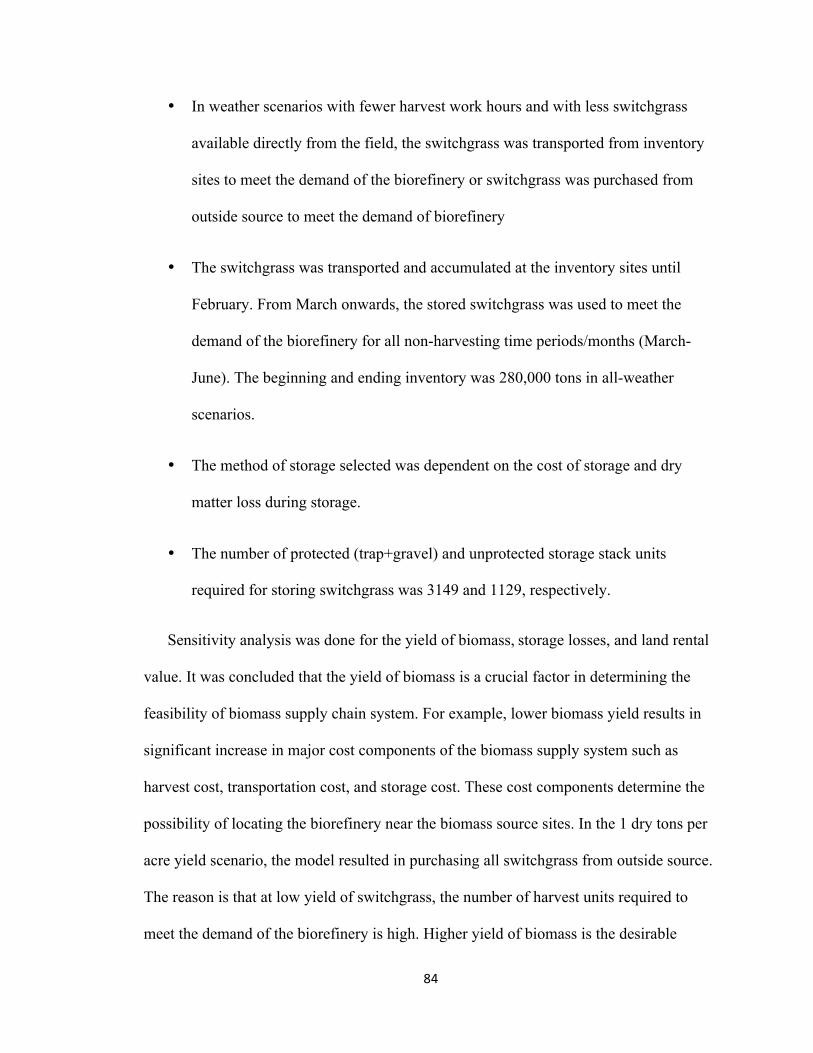
84

• In weather scenarios with fewer harvest work hours and with less switchgrass

available directly from the field, the switchgrass was transported from inventory

sites to meet the demand of the biorefinery or switchgrass was purchased from

outside source to meet the demand of biorefinery

• The switchgrass was transported and accumulated at the inventory sites until

February. From March onwards, the stored switchgrass was used to meet the

demand of the biorefinery for all non-harvesting time periods/months (March-

June). The beginning and ending inventory was 280,000 tons in all-weather

scenarios.

• The method of storage selected was dependent on the cost of storage and dry

matter loss during storage.

• The number of protected (trap+gravel) and unprotected storage stack units

required for storing switchgrass was 3149 and 1129, respectively.

Sensitivity analysis was done for the yield of biomass, storage losses, and land rental

value. It was concluded that the yield of biomass is a crucial factor in determining the

feasibility of biomass supply chain system. For example, lower biomass yield results in

significant increase in major cost components of the biomass supply system such as

harvest cost, transportation cost, and storage cost. These cost components determine the

possibility of locating the biorefinery near the biomass source sites. In the 1 dry tons per

acre yield scenario, the model resulted in purchasing all switchgrass from outside source.

The reason is that at low yield of switchgrass, the number of harvest units required to

meet the demand of the biorefinery is high. Higher yield of biomass is the desirable

85

parameter for the biorefinery feasibility. Additionally, not much variation was observed

in 2 and 3 dry acre per ton weather scenario. The yield greater than 3 dry tons per acre

can provide significant cost savings for biomass supply system. The dry matter loss and

land rental values affected the cost to the biorefinery. Other inputs to the model can also

be changed and their effect on decision variables can be evaluated for particular region or

location. The direction for future research should be to consider different types of

biomass feedstocks and conversion processes into the model.

86

References

[1] Groover G. What Does that Bale of Hay Really Cost? 2009. [2] Yu Y, Bartle J, Li C-Z, Wu H. Mallee biomass as a key bioenergy source in

Western Australia: Importance of biomass supply chain. Energy and Fuels. 2009;23(6):3290-3299.

[3] Turhollow A, Wilkerson E, Sokhansanj S. Cost methodology for biomass feedstocks: Herbaceous crops and Agricultural residues. Oak Ridge Natinal Laboratory, US Department of Energy, 2009.

[4] Miller E. Dry matter loss in large square bales stored in Panhandle, Oklahoma. B. Sharma. Oct 22 2012.

[5] Khanchi A. Drying and storage of switchgrass [Dissertation]. Biosystems and Agricultural Engineering, Oklahoma State University, Stillwater; 2012.

[6] USDA. Chariton valley biomass project. Chariton Valley RC&D;2002. [7] Mapemba LD. Cost to deliver lignocellulosic biomass to a biorefinery

[Dissertation]. Oklahoma State University, 2005. [8] Ampong-Nyarko K, Murray CL. Utility of forage grass nutrient composition

databases in predicting ethanol production potential. Journal of Biobased Materials and Bioenergy. 2011;5(3):295-305.

[9] OSU. Realistic expectations for Switchgrass c2010 [cited 2011 Jan 22]. Available from: http://switchgrass.okstate.edu/whatisswitchgrass/index.htm.

87

APPENDIX-A

88

The taxonomy classifications of journal articles reviewed are as follows:

The taxonomy classifications of journal articles reviewed are as follows:

Decision level

A supply chain consists of a natural hierarchy of decision making processes,

which includes: strategic (long-term,), tactical (medium-term) and operational (short-

term) decisions based on their level of significance [1]. Figure A-1 presents the BSC

decision levels.

Figure A-1 Decisions related to biomass supply chain [2-5]

Supply chain structure

The supply chain structure defines the arrangement of different organizations or

entities in the supply chain. The supply chain structure is classified as convergent,

divergent, conjoined, and networked as described in Table A-1 [6]. This section identifies

the BSC structure considered by researchers.

89

Table A-1. Supply chain structural classification (reproduced from Beamon and Chen [6]) Classification type Explanation Example

Convergent Each node or facility in supply chain has at most one successor but many predecessors

Divergent Each node in the supply chain has one predecessor but many successors

Conjoined Convergent and divergent structure is combined in an order and provide a single connected structure

General (Networked) The structure which is not convergent, divergent or conjoined it is the general structure

Modeling approach

Mathematical models are equations or sets of equations, which describe real

world phenomena [7]. Different types of modeling approaches are used depending on the

type of application. The classification presented by Mula et al. [8], Keramati and Eldabi

[9] and Min and Zhou [10] was used. Figure A-2 represents the classification of supply

chain models.

In the deterministic models, the parameters are known and are fixed with

certainty. They are further classified into single-objective and multiple-objective models.

90

In stochastic models, the parameters are uncertain and random; they are also called

probabilistic models. They are sub-classified into optimal control theoretic and dynamic

programming models. Hybrid models have elements of both deterministic and stochastic

models. The models include inventory-theoretic and simulation models. The IT-driven

models integrate and coordinate various phases of supply chain planning on real time

basis using application software. This helps to enhance the visibility throughout the

supply chain [9, 10].

Figure A-2. Modeling approach types and codes

Quantitative performance measure

One of the important components in supply chain design and analysis is the

development of an appropriate performance measurement for the system. These

parameters measure the efficiency of a system along with comparing alternatives. The

performance measures are classified into qualitative and quantitative [7, 11]. The

quantitative performance measures are expressed numerically. The qualitative

91

performance measures are not generally used in BSC; therefore, in the present study only

quantitative performance measures are considered. Figure A-3 represents the quantitative

performance measures with their codes.

Figure A-3. Quantitative performance measures and codes

Shared information

This section identifies the shared information between entities in the BSC. In the

present review, entities, end-products, biomass type, and cost information provided by

researchers for different operations of BSC was considered. This information is crucial

for efficient supply chain design.

92

Entities and end-‐products

This section identifies the entities, end products, and biomass types considered in

BSC models. Table A-2 describes the entities in the BSC model. The end products are

bioethanol, bioelectricity, biodiesel, and heating, power and cooling or a combination.

Table A-2. Entities considered in BSC structure Entity name Description Biomass Source Site / Sites (BSS/BSSs)

Site from where biomass is harvested

Collection Site (CS/CSs) Site where biomass or biofuel is collected and stored

Transshipment Site (TS/TSs) Site required when using different modes of transportation

Pre-Processing or conditioning Site (PP/PPs)

Site where certain operations are performed on biomass influencing its specific attributes for improving transport or storage characteristics. The processes include pelleting, size reduction, and drying of biomass. The pretreatment can occur at different locations in the supply chain, unless specialized equipment is required that cannot be installed at existing locations. A special pretreatment site is required in that case [12]

Final Processing Site / Sites (PS/ PSs)

Site where biomass is converted to bioenergy or biofuels

Other entities

Intermediate-Processing Site/Sites (IPS/IPSs)

Site where intermediate products are produced, for example bio-oil

Blending Site/Sites (BL/BLs) Site were ethanol is blended with gasoline

Distribution Sites/Sites DS/DSs Site from where the biofuel /bioenergy is collected and is distributed to final customer

Demand Centers or Consumers (CO/COs) for biofuels/bioenergy

Site for the utilization of the final product such as blended gasoline, electrical energy, heat etc.

93

Novelty

This section describes the author’s contribution to the BSC modeling design and

analysis in comparison to rest of the literature. The focus is on the modeling approach

and the major findings of the article.

Application

This section describes the case studies or numerical examples considered by the

other researchers to support and present the applicability of their model.

Assumptions, limitations, and future work This section identifies the assumptions, limitations, and future work proposed by

the research articles. The BSC models make some basic assumptions for developing the

constraints such as land availability (acres harvested for biomass will not exceed the

available acres), biomass availability. Such assumptions used for building the constraints

for the model are not identified. Only the assumptions that are explicitly stated in the

work are identified and reported.

Results and discussion

Thirty journal articles on the BSC modeling were reviewed and are shown in

Table A-3. Table A-4 and Table A-5 present the distribution of references according to

the journal and the year of publication. It was observed that maximum references were

obtained from Biomass and Bioenergy (6 articles, 20.00 %), and Bioresource Technology

(4 articles, 13.33 %). The maximum number of published articles was in the year

2011(13 papers), which indicates growing interest in BSC design and analysis.

94

Table A-3. Reviewed work References Author [13] Cundiff, 1997 [12] De-Mol et al., 1997 [14] J. Nagel, 2000 [15] Tembo et al., 2003 [16] Tatsiopoulos and Tolis, 2003 [17] Freppaz et al., 2004 [18] Gunnarsson et al., 2004 [19] Morrow et al., 2006 [20] Mapemba et al., 2007 [21] Dunnett et al., 2007 [22] Mapemba, et al., 2008 [23] Vlachos et al., 2008 [24] Frombo, et al., 2009 [25] Zamboni, et al, 2009 [26] Rentizelas, et al., 2009 [3] Eksioglu, et al., 2009 [27] Yu, et al., 2009 [28] Huang, et al., 2010 [29] Papapostolou, et al., 2010 [30] Kim, et al., 2010 [31] Kim, et al., 2010 [32] Dal-Mas, et al., 2011 [33] Zhu, et al., 2011 [34] Marvin, et al., 2011 [35] An, et al., 2011 [36] Bai, et al., 2011 [37] You, et al., 2011 [38] You and Wang, 2011 [39] Lam, et al., 2011 [40] Zhu, et al., 2011 [41] Kim, et al., 2011 [42] Chen and Fan, 2011

95

Table A-4. Distribution of references according to the journal of publication (Published till January 2012) Journal References % Total Biomass and Bioenergy 6 20.00 Bioresource Technology 4 13.33 Transportation Research 3 10.00 Energy 2 6.67 Energy and Fuels 2 6.67 Industrial and Engineering Chemistry Research 2 6.67 Manufacturing Engineering 1 3.33 American Institute of Chemical Engineers 1 3.33 Chemical Engineering Science 1 3.33 Computer Aided Chemical Engineering 1 3.33 Computers and Chemical Engineering 1 3.33 Computers and Industrial Engineering 1 3.33 Ecological Engineering 1 3.33 Environmental Science Technology 1 3.33 Journal of Agricultural and Resource Economics 1 3.33 Netherlands Journal of Agricultural Science 1 3.33 Review of Agricultural Economics 1 3.33

30 100.00

Table A-5. Distribution of journals according to the year of publication (Published till January 2012) Year References % Total 1997 2 6.67 2000 1 3.33 2003 2 6.67 2004 1 3.33 2006 1 3.33 2007 1 3.33 2008 2 6.67 2009 5 16.67 2010 1 3.33 2011 13 43.33 2012 1 3.33

30 100.00

96

Decision level

The decision levels are strategic, tactical, and operational, depending on their

effect in terms time and duration [8]. Table A-6 describes the BSC strategic decisions

codes. Table A-7 and Table A-8 classify the works reviewed in terms of strategic

decisions, and tactical and operational decisions. The majority of works focused on

strategic decisions related to location and capacity of plants and network design. The

tactical and operational decisions were related to material flow, storage and pre-treatment

methods, harvesting units, transportation units etc. All reviewed works have the ability to

make tactical decisions on material flow in a time period. The work by Dal Mas et al,

You et al, You and Wang [32, 37, 38] assessed the environmental impact of bioenergy

production by calculating total emissions. The social impact in terms of accrued jobs was

estimated by You and Wang [38]. It was observed that recent studies are addressed the

critical issues of sustainability and socioeconomic impacts of BSC. The results from the

review also indicate that over the years, the mathematical models have improved the

decision making capabilities. The models are developed for the entire biofuel supply

chain and use heuristic algorithms to deal with the complexity of the problem.

Table A-6. Supply chain strategic decisions codes Decision Code Sourcing SO Production technology PT Biomass types BT Location and capacity of processing site LCPS Location and capacity of blending site LCBS Location and capacity of inventory site LCIS Location and capacity of pretreatment site LCPPS Location and capacity of distribution site LCDS Sites serving a particular site (example BSS serving the particular CS) SPS Transportation mode TM Supply and demand contracts SADC Network design ND Sustainability SUS

97

Table A-7. Strategic decision level of the reviewed work References SO PT BT LCPS LCIS LCBS LCPPS SPS TM SADC ND SUS [13] x x [12] x x x [14] x x x x x x [15] x x x [16] x x x x [17] x x x [18] x x x x [19] x x x [20] x x x [21] x x [22] x x x [23] x x x x [24] x x x [25] x X x x x [26] x x X x [3] x x x x x [27] [28] x x [29] [30] x x x [31] x x x x [32] x x x x [33] x x x [34] x x [35] x x x x x [36] x x x [37] x x x x x x [38] x x x x x [39] x X x [40] x x x x x [41] x x x x [42] x x x

98

Table A-8. Tactical and operational decisions level of the reviewed work

Ref. Pretreatment method

Collection method

Biomass harvested

Biomass stored

Biomass transported

Biofuel transported

Biomass Processed / bioenergy produced

NHU* NTU* Others

[13] x x [12] x x x [14] [15] x x x x [16] x x x x outsourcing [17] x [18] x x x [19] x x [20] x x x x x [21] x x x x x [22] x x x x x [23] x [24] x [25] X X X x [26] x [3] x x x x x [27] x x [28] x x x x [29] x x

[30] x x x x x

[31] x

Intermediate product flow and processed amount

[32] x x x x [33] x x x x x [34] x x x x [35] x x [36] x x

[37] x x x x x x

Biofuel stored, by-product produced, and accrued jobs

[38] x x x x x x

Biofuel and intermediate product stored, intermediate product flow

[39] x x Intermediate product flow

[40] x Residue produced

[41] x x x x

Intermediate product flow and processed

[42] x x x Unmet demand

*NHU=Number of harvest units, NTU=Number of transportation units

99

Supply chain structure

The reviewed works was classified according to their supply chain structure type

as previously described in the review methodology. The vast majority of the reviewed

works presents a network-like structure (Table A-9). The structure mainly combines the

biomass source sites, collection sites, and final processing sites with some works

consisting of transshipment sites, pre-processing or conditioning sites, intermediate-

processing sites, blending sites, and demand points for bioenergy. Only three reviewed

works considered biomass moving to a single bioenergy site and formed a convergent

structure [13, 27, 29]. Two reviewed works use the conjoined structure of BSC [16, 43].

The optimal network design is crucial for efficient and effective delivery of BSC system.

Modeling approach

Table A-10 presents the distribution of the reviewed works according to the

modeling approach. The vast majority of the works reviewed followed the mixed integer

linear programming approach. Five references followed the linear programming approach

[44]; whereas, two references used the multi-objective integer linear programming

approach. The uncertainty in BSC was accounted for by using the stochastic modeling.

Three references used the stochastic modeling approach; whereas, one reference used the

hybrid modeling approach. The stochastic modeling approach handles uncertainty and

makes the decisions more realistic and robust. The BSC has various sources of

uncertainty such as biomass supply, demand, government incentives, etc. The models that

incorporate uncertain factors tend to become complex and difficult to solve. One of the

challenges faced by the biofuel industry is to develop a model that accounts for

uncertainty and can handle large scale problems.

100

Table A-9. Supply chain structure of the reviewed work References Convergent Divergent Conjoined Network [13] x [12] x [14] x [15] x [16] x [17] x [18] x [19] x [20] x [21] x [22] x [23] x [24] x [25] x [26] x [3] x [27] x [28] x [29] x [30] x [31] x [32] x [33] x [34] x [35] x [36] x [37] x [38] x [39] x [40] x [41] x [42] x

101

Table A-10. Modeling approach of the reviewed work References LP MILP/ ILP INLP MOILP SP HYB [13] x [12] x [14] x [15] x [16] x [17] x [18] x [19] x [20] x [21] x [22] x [23] x [24] x [25] x [26] x [3] x [27] [28] x [29] x [30] x [31] x [32] x [33] x [34] x [35] x [36] x [37] x [38] x [39] x [40] x [41] x [42] x

Quantitative performance measure

Table A-11 presents the distribution of reviewed works according to the

quantitative performance measure. The majority of the reviewed works presents the cost

minimization as the quantitative performance measure. Thirteen references used the

profit or revenue maximization and the net present worth maximization as the purpose of

102

the work. Morrow et al. [19] established minimization of the volume-transportation

distance as the objective function. The authors claim that minimization of transportation

cost was not feasible due to unavailability of data on fixed and variable cost for different

modes of transportation. You et al. [37] developed a multi-objective model for

minimizing annualized total cost, minimizing greenhouse gas (GHG) emissions, and

maximizing the number of accrued jobs. You and Wang [38] proposed the same

formulation as You et al. [37] except the objective function of maximizing the number of

accrued local jobs was not included in the study. The purpose of Mas et al. [32] was

maximizing profit and minimizing the expected economic losses under adverse

conditions. The multi-objective modeling approach has potential to incorporate

economic, social, and environmental impacts of BSC, but advanced techniques are

required to solve complex mathematical formulations.

103

Table A-11. Quantitative performance measure of the reviewed work References CM PM NPWM Others [13] x [12] x [14] x [15] x [16] x [17] x [18] x [19] Volume-transportation distance minimization [20] x [21] x [22] x [23] x [24] x [25] x [26] x [3] x [27] x [28] x [29] x [30] x [31] x [32] x Risk minimization [33] x [34] x [35] x [36] x [37] x GHG emissions and number of local jobs minimization [38] x GHG emissions minimization [39] [40] x [41] x [42] x

Shared information Entities and end-‐products Table A-12 presents the distribution of reviewed works according to the entities,

end-products, and biomass type. The majority of the works reviewed considered multiple

types of biomass for bioethanol production. Using multiple types of biomass tends to

reduce overall cost of the system. But production technology for using multiple types of

104

biomass with varying physical and chemical characteristics poses major technical

challenges [43]. Nine references were for heating, electricity, or combined heat and

power production from biomass. Most of these studies were done in Europe. As the three

countries that form the world’s most intensive cogeneration economies are in Europe.

The U.S. is also aiming for 20% of generation capacity using cogeneration technology by

2030 [45]. These technologies are not fuel specific and help in developing a balanced and

sustainable energy portfolio [46]. The entities considered by almost all references were

the biomass source sites, and processing sites. Some of the studies focused on integrated

view of BSC considering all the entities from biomass supply to end user/demand centers.

Integrated view of biomass/ biofuel supply chain is economical as the activities are

highly interconnected [47]. The upstream decisions are related to biomass production,

biomass delivery, and production sites, and the downstream decisions are related to

production distribution to the end-user demand centers. The upstream decisions have

significant impact on the later activities in the supply chain [32, 47]. Therefore, it is

important to consider all entities of the biomass/ bioenergy supply chain system in its

design and analysis.

This section also considers information about costs, biomass availability, and

production capacities for the reviewed articles. Majority of the works shared information

on biomass availability, production capacities, and production rates. The cost information

shared by the references is presented in Table A-13. Vast majority of works reviewed

provided biomass cost, processing cost, and transportation cost. Depending on the entities

considered by the model the additional cost elements were added. Three references also

included the penalty cost for not meeting demand. Adding penalty cost forces the model

105

to meet the demand. But in the real world situation there will be scenarios when the

demand could not be met due to uncertainties in weather or biomass supply. The

information on type of constraints developed by reviewed works was also evaluated.

Demand, flow balance, capacity, and logical constraints were the most common types of

constraint for the BSC modeling system. Three references included constraints for

ensuring sustainability by limiting the use of biomass to prevent negative impact on food

production [24, 30, 32]. Ensuring sustainability in BSC is critical for the long-run

successful operations of biorefineries. It is important to identify sustainable resources at

local and regional level, and cost-effectively integrate them with processing plants, while

identifying constraints for different supply chain designs. Rentizelas et al. [26] includes a

social constraint for safe distance of the conversion plant from demand sites.

106

Table A-12. Entities and end-products of the reviewed work Ref. Biomass Type End-product Entities

[13] Switchgrass Bioethanol BSSs, CSs, PS [12] Multiple biomass types Biofuel BSSs, CSs, PPs, PSs [14] Wood, straw, biogas, rapeseed Heating generation or power

generation or co-generation BSSs, PSs , DSs, COs

[15] Multiple biomass types Bioethanol BSSs, PSs [16] Cotton-plant stalks Combined heat and power BSSs, CSs, PSs [17] Forest biomass Thermal and electric energy BSSs, PSs, DPs [18] Forest residue Heating plants BSSs, CSs, PSs [19] Switchgrass and corn Bioethanol PSs, DPs [20] Multiple biomass types Bioethanol BSSs, PSs [21] Miscanthus Heat BSSs, CSs, CPPs, PS [22] Multiple biomass types Bioethanol BSSs, PSs [23] Waste biomass Bioenergy BSSs, CSs, PPs , PSs [24] Forest biomass Thermal energy and electricity BSSs, CSs, PSs [25] Multiple biomass types Bioethanol BSSs, PSs, DPs [26] Multiple biomass types Electricity, heating and cooling BSSs, CSs, PSs, DPs [3] Multiple biomass types Bioethanol BSSs, CSs, PSs, BLs [27] Mallee Bioenergy BSSs, PSs [28] Multiple biomass types Bioethanol BSSs, PSs, DPs [29] Multiple biomass types Heat, power, and biofuel or all BSSs, PSs [30] Multiple biomass types Bioethanol BSSs, PSs, DPs [31] Multiple type biomass Gasoline and Biodiesel BSSs, PSs, IPSs, DPs [32] DDGS Bioethanol BSSs, PSs, BLs,DPs [33] Switchgrass Bioethanol BSSs, CSs, PSs [34] Agricultural residues Bioethanol BSSs, CSs, PSs [35] Multiple biomass types Bioethanol/Biofuel BSSs, CSs, PPs, PSs, DSs, DPs [36] Biomass Bioethanol BSSs, PSs, DPs [37] Agricultural residue, energy crops

and wood residues Bioethanol BSSs, CSs, PSs, DPs

[38] Cellulosic biomass Gasoline & Biodiesel BSSs, IPSs, PSs, DPs [39] Multiple biomass types Biofuel BSSs, CSs, IPSs, PSs, DPs [40] Perennial grasses and agricultural residue Bioethanol BSSs, CSs, PPs [41] Multiple biomass types Gasoline and Biodiesel BSSs, PSs, IPSs, DPs [42] Bio-waste Bioethanol BSSs, PSs, BL/BLs, DPs

107

Table A-13. Shared information on cost of the reviewed work Ref. *BC *PTC *CC *TC *IC *PC *O [13] x x x Construction/expansion of storage

facility, Penalty cost for demand shortage

[12] x x x x [14] x x Capital and operating cost of facility,

fuel costs, disposal costs for waste-products, cost of external heat, distribution cost

[15] x x x x Capital and operating cost of facility [16] x x x x x Capital cost of facility [17] x x x Capital cost of facility, energy

distribution cost [18] x x x x x [19] x x [20] x x x x Capital and operating cost of facility,

cost of harvest unit [21] x x x x x [22] x x x x Capital and operating cost of facility,

cost of harvest unit [23] x x Capital and operating cost [24] x x Capital and operating cost [25] x Capital cost of facility [26] x x x x x [3] x x x x [27] x x x [28] x x x Capital cost of facility, penalty cost

for demand shortage, loading and unloading cost

[29] x [30] x x x Capital cost of facility [31] x x Capital and operating cost of facility [32] x x x Capital and operating cost of facility [33] x x x x Cost of owning and operating harvest

unit, Capital cost of facility , handling residue cost

[34] x x x x Capital and operating cost of facility [35] x x x Capital cost of facility [36] x Capital cost of facility [37] x x x x Capital and operating cost of facility [38] x x x x Capital and operating cost of facility,

distribution cost, cost of technology, [39] x Capital and operating cost of facility [40] x x x x Capital and operating cost of facility [41] x x Capital and operating cost of facility [42] x x x Capital and operating cost of facility,

penalty cost for demand shortage *BC-Biomass cost, PTC-Pre-treatment cost, CC-Collection/ handling cost, TC-Transportation cost, IC-Inventory cost, PC-Processing cost, O-Others

108

Novelty Table A-14 describes the novelty and contribution of the reviewed work to the

BSC modeling, design, and analysis. It was observed that modeling techniques and

solution capabilities have improved significantly over the years. The mathematical

models have been developed with capabilities of numerous parameters along with

addressing economic, environmental, and social constraints.

Table A-14. Novelty of the reviewed work Ref. Novelty

[13] A two-stage linear programming model with recourse was developed. Uncertainty in biomass yield during growing and harvesting seasons was addressed by considering 4 weather scenarios. The model provides realistic cost estimates for biomass delivery to biorefinery.

[12] A network structure model solved by integrating the three sub-models (biomass flows without pretreatment, biomass flows with pre-treatments in a separate pre-treatment site, biomass flow with pre-treatment possible in every node) into a Knapsack model. A comparison was made between the optimization model and simulation model. It was concluded that both optimization and simulation models provide insight into the costs of biomass supply. The optimization model resulted in best network structure, and simulation model provides more insight on costs involved.

[14] An integrated optimization model for energy production considering three types of operating companies was developed. The model considered three dimensions: technology, location, and time. The model provides a comprehensive scenarios analysis with a base scenario consisting of prices of fuels, reduction of heat consumption, co2 emissions, investments costs, central and individual conversion plants etc. The model can simulate the political, economical, ecological circumstances or future aims, by making changes to the base scenario.

[15] A comprehensive multi-region, multi-period integrated model was developed. The model considered biomass harvest window, field losses, storage losses, fertility regime, and multiple output products.

[16] An integrated planning model was developed. The model analyzed centralized and decentralized structure for CHP-cogeneration along with considering two scenarios for collection and transportation: third party companies and the farmers undertake collection and transportation. Different power plant capacity scenarios were also considered. The model has potential for developing future business strategies for biomass.

[17] A Decision Support System (DSS) for forest biomass, combing the Geographical Information System (GIS) techniques along with mathematical programming and database was developed. The DSS system can be used for biomass exploitation in a region, determining the location and capacity of plants, and evaluation of overall performance of the system. The system exploits the biomass areas ensuring sustainability.

[18] A two-level facility location problem was modeled and solved using heuristics approach based on sequential LP. The harvest areas considered were self-owned or contracted. The model can be used for better planning and testing of different alternative scenarios. The model has capability of analyzing strategic planning situations such as a company competing for a new contract and wants to submit the contract prices, the company want to conduct sensitivity analysis on variation in demand etc.

[19] A minimization transportation-distance optimization model was developed considering economic costs of distribution of different ethanol blends to all metropolitan areas in the U.S. It was concluded that an effective and efficient, transportation system and processing technology is required to make ethanol use feasible and competitive in the long run.

[20] The model is an extension of the model developed by Tembo et al. [15]. The total number of harvest units was considered. The model considered restrictions in harvest schedule due to harvest season length and frequency of harvest on CRP land. The model provides insights into how the policies that restrict the harvest season length and frequency of harvest can affect the cost of biomass supply.

[21] A State-task-network approach was presented for design and scheduling operations for biomass to heat supply chain. To demonstrate the effectives of the approach the optimal designs from the model were compared to those derived from heuristics based strategies. It was concluded that potential economic benefits can be achieved by applying system optimization methods. The results indicated that 5-25 % improvements in cost minimization objective can be obtained.

109

Table A-14. Novelty of the reviewed work (continued) Ref. Novelty

[22] The model was an extension of model developed by Tempo et al. [10]. The model incorporates number of harvest days per month based on the historical weather patterns. The storage losses were associated with location and time of storage. The results from previously developed model were compared to the present model. The assumptions made for the harvest units affect the results from the model. The present model provides more realistic and reliable estimates on harvest costs by considering number of workdays in comparison with the previously developed models which considered harvest cost as fixed cost per mg harvested.

[23] A quantitative model was developed for making strategic decisions of identifying nodes for different operations of BSC and determining the biomass flow in the network.

[24] Environmental decision support system consisting of GIS interface, database and optimization module was developed. A user-friendly interface allows developing and running scenarios for strategic planning.

[25] The spatially explicit model was developed considering cost and environmental impact by GHG emissions. [26] A decision support system with hybrid optimization method was developed. The demand driven system-

wide optimization was done. The model provides practical tool for investors to evaluate and optimize system to achieve cost-effectiveness with incorporating the real energy demand.

[3] A network design problem capable of making strategic, tactical and operational decisions was developed. The model minimizes system wide cost and intends to achieve significant cost saving.

[27] A discrete mathematical model was developed for Mallee biomass. The model considers differences between the on-farm transport and road-transport and also considers tortuosity of roads.

[28] A mathematical model which integrates the spatial and temporal dimensions was developed. The authors states that optimizing entire supply chain provides better understanding of tradeoffs between the spatial and temporal dimensions.

[29] A generic optimization model for biomass conversion to heat, power or biofuel production was developed. [30] An optimization model using 4N and 8 N neighborhood representation modeling approach was developed.

The model can solve large scale network problems. [31] An optimization model considering pyrolysis process and Fischer Tropsch process for forest biomass

conversion was developed. The model compares the centralized and decentralized network structure with regard to profit per ton at different demand scenarios. The model can contribute to the development of process systems design for systems other than biofuel biorefineries.

[32] A dynamic, spatially explicit, and multi-echelon model was developed. The model had two objective functions of maximizing profit and minimizing losses for adverse conditions. The model consisted of scenarios for corn cost and selling price of ethanol. The model provides best network structure with regard to biomass source sites, production sites, and transportation logistics.

[33] A model was developed for strategic and tactical level planning for switchgrass supply chain. The model considered harvesting and non-harvesting seasons and all the unique features of switchgrass. A well-designed logistics system results in increase in the unit profit of bioenergy

[34] The model was developed for 9-state region in the Midwestern U.S. and concluded that the region has the capacity to run a 4.7 BGY cellulosic ethanol plant.

[35] A time staged multi-commodity model was developed. The model provides compressive view of both upstream and downstream echelons in BSC. The model can be used by the manufactures to determine the most profitable scenario. The model can be used by the Government policy makers to determine the policies that are most efficient to successful implementation of biofuel industry.

[36] The model is an integration of traffic assignment model and fixed-charge facility location problem. The model explicitly incorporates shipment routing decisions and traffic congestion impact into facility location design model to determine biorefinery location and transportation of ethanol. The model is solved using different approaches of Lagrangian relaxation (LR), linear programming relaxation, branch and bound, convex combination. The LR approach solved the model in less time and resulted in good feasible solutions.

[37] A life cycle analysis technique was integrated with multi-objective multi-period optimization model to evaluate alternatives to achieve economic, environmental, and social improvement. The problem was formulated as bi criteria optimization model and solved with e-constraint method. The model considers seasonality of biomass feedstock, biomass loss with time, geographical diversity, biomass variability, feedstock density, moisture content, conversion technologies and byproducts, infrastructure, demand distribution, tax subsidies, policies, and regional economic conditions. Biochemical and thermochemical pathways were considered for conversion.

110

Table A-14. Novelty of the reviewed work (continued) Ref. Novelty

[38] The life cycle analysis technique was integrated with multi-objective, multi-period model with economic and environmental objectives. The emissions during all stages from “field-to-wheel” were considered. The model considers seasonality of biomass feedstock, biomass loss with time, geographical diversity, biomass variability, moisture content, conversion pathways, infrastructure, demand variation, and government incentives. The multi-objective model resulted in Pareto-optimal curve taking into account economic, and environmental objectives. The curve indicates the variation in optimal annualized cost and the biomass to liquid processing network change with different environmental performances.

[39] An optimization model considering 4 layers supply chain structure was developed. Different techniques such as reducing connectivity in the network, removing unnecessary variables and constraints from the zero-flows, and merging of zones within the network was used for model size reduction. It was found that these techniques reduce computational time significantly with little loss in accuracy.

[40] A multi-commodity network flow model was developed. [41] A two-stage mixed integer stochastic model was developed. A methodology consisting of sequence of steps was

proposed to deal with uncertainty in parameters. First, the single nominal scenario was optimized and then the value of objective function for extreme values of 14 major parameters was analyzed. Then the high impact parameters were selected and multiple scenarios were generated and analyzed for optimal design. Robustness analysis and global sensitivity analysis were done for the comparison of nominal design vs. scenario design. The methodology was successful in dealing with parameter variation and uncertainty.

[42] A two stage SP model was developed. The feedstock supply and demand uncertainty was dealt by considering set of possible scenarios. The SP modeling increased the computational burden and could not be solved using commercial software. Decomposition methods reduced the problem size and tend to provide realistic estimates on cost and network design. It was concluded that advanced system based approaches will provide better design and analysis of BSC.

Application

Table A-15 presents the practical application or numerical examples of the

reviewed works. The section also presents the major findings of the reviewed work

related to the particular application or the numerical example. This section provides an

outline for the scale and validation of the models developed by researchers. The majority

of the works presented a case study for a region, with some studies assuming the data and

others using realistic data sets. .The extensive use of case studies to validate the model

shows that the models have practical applicability when used with regional or local

constraints.

111

Table A-15. Application and important findings of the reviewed work Ref. Application and important finding [13] A case study of bioethanol plant located in a hypothetical Piedmont county was presented. 20 switchgrass

producers with each producer having 4 to 7 storage location were considered. Switchgrass from 3 to 10 fields was stored at each storage location. Cost estimates for switchgrass delivery were estimated along with recommendation of shipping and capacity expansion schedules for each producer.

[12] A case study for province of North-Holland in Netherlands was developed. Biomass types: thinning and restwood, pruning, waste wood, sewage sludge or waste paper; Transport modes: road, rail or water transport; Pre-treatment of biomass: particle size reduction, drying; Location of energy plant: 4 possible locations. Authors concluded centrally located energy plant is optimal with respect to cost. Road and water transportation modes are desirable and pre-processing should be done at energy plant.

[14] A practical application of model to a rural municipality of the Brandenburg area with 660 inhabitants was developed. The author concluded that CO2 emissions could be decreased up to 25% by increasing the use of biomass. The results indicated that supply of energy based on biomass is possible. The author also described the factors that can improve the economic viability of biomass use.

[15] A case study for 77 counties with 11 potential biorefinery locations for the state of Oklahoma was developed. The base model results showed that 5 large biorefineries (100 million gallons per year), 1 medium sized biorefinery (50 million gallons per year) could be developed in the particular counties of Oklahoma. The results also indicate that biomass should be harvested from June to October. 8 alternative scenarios to determine a breakeven price of ethanol: doubling land cost, doubling biorefinery investments cost, doubling per mile feedstock transportation cost, changing project life to 10 years, changing project life to 20 years, using discount rate of 5% and 25 % were considered.

[16] A case study for Thessally with almost 30,000 cotton producers and the biggest cotton harvesting area of Greece and Europe was developed. The results indicate that the most economical method for transporting biomass requires farmers involvement in the logistics system. It was also observed that the economies of scale can be achieved with increasing capacity of transportation vehicles. The warehousing method suggested was closed depots and drying, and was found to be more cost-effective than baling.

[17] A case study for Vol Bormida (Savona district, Italy) was developed. The area was divided into 370 parcels containing 1 of the 4 main types of biomass (beech, oak, chestnut, and conifer) and the biomass waste from 10 industrial sites was also considered. The results showed that 16% of the energy demand can be satisfied at a reasonable cost with the available biomass. The results showed that energy production fulfills local thermal and energy demands while electric energy was only produced during low energy demand at any plant.

[18] A case study for Swedish entrepreneur of Sydved Energileveranser AB was developed. Sydved is the largest supplier of biofuel energy in Sweden. The case study was developed for the north region of company consisting of Värmland, Närke, Södermanland, Stockholm, Uppland and Västmanland counties. Different scenarios were developed considering increased demand, restriction on storage levels, more customers, changing chipping capacity, and adding new terminals. It was found that the byproducts need to be stored at the terminals and once the forest biomass is chipped, it should be directly transported to heating plant. The results could not be compared to the manual solutions. The authors suggest that the manual solutions work fine at the beginning of the year but towards end of the year, these solutions are not valid and become problematic. The optimization model provides solution for entire year and should be used for strategic and tactical planning.

[19] A case study for the Metropolitan areas in the United States was developed. The shipments of corn and cellulosic ethanol blends (E5, E10, and E16) to 271 largest Metropolitan Statistical Areas (MSA) was considered. Different scenarios such as E5, E10, E16, and ethanol and switchgrass yields variation were studied. It was concluded that pipelines are the most effective method for shipping ethanol. Increased use of ethanol can have positive impact on energy security, economy, and environment. But the total infrastructure required for such changes is problematic and challenging.

[20] A case study for the 52 Kansas counties, 77 Oklahoma counties and 32 Texas counties was developed with perennial grasses including prairie grasses established on CRP acres in these regions. Results showed that 11 counties were considered as potential biorefinery locations sites. The model was executed for 9 different scenarios considering different policies of harvest days and frequency of harvest and biorefinery size. It was found that restriction on harvest days and frequency of harvest increases the harvest, storage, and transportation costs. With the increase in biorefinery size, the number of harvest units required also increases.

[21] A model was tested for a hypothetical heat plant with 20 MW peak output using surrounding agricultural resources within approximately 1225 square km area. Two distant spatial locations were considered: a farm which consists of cultivation, harvesting, storage, decentralized drying, and chopping process, and a centralized conversion plant included storage, centralized chipping, forced drying, and combustion processes. The results indicate that land, cultivation, and harvesting cost account for the major portion of supply chain economics.

112

Table A-15. Application and important findings of the reviewed work (continued) Ref. Application and important finding [22] The same case study as presented by Gunnarsson et al. [15] was considered. 26 harvest units were found to meet

the demand of biorefinery. Whereas, the conventional model resulted in requirement of 55 harvest units. It was concluded that associating harvest capacity with number of harvest days available in a month provides realistic estimates of cost.

[23] A case study for wood industry located within the region of central Macedonia, Greece was developed. 3 echelons were considered for the study with 7 collection points, 2 potential storage nodes, and 1 final destination. Wood based particle boards and wheat straw were the biomass resources. Results indicate that biomass should be directly transported to plant.

[24] A case study for Val Bormida Province consisting of 2300 parcels was considered. The biomass plant location was at the Cairo Montenotte district. It was found that fast pyrolysis and diesel engine technology plants have fewer benefits compared to other technologies. The fluid bed gasification received the worst economic value. The grate firing combustor and steam cycle technology requires less supervision and could be easily managed.

[25] A case study was developed for corn-based ethanol production in northern Italy. 4 ethanol plants of varying capacities at Venice Harbor, Porto Viro, Tortona, and Trieste were considered. The first 2 facilities will start production first as they are under construction. Two demand scenarios with 3% penetration by energy content for the year 2009 and 5.75 % penetration by energy content for the year 2010 were considered. The results indicate that to meet the 2009 demand, the ethanol plants of 120,000 and 150,000 tons /year capacity should be located at Venice and Milan, respectively. For the 2010 scenario, it was suggested that additional capacity of 240,000 tons/year for Venice plant and construction of a same capacity plant at Milan. The cost saving was found to be of 8% in comparison with the likely planned scenarios.

[26] A case study for the district of Thessaly, Greece was considered. The results showed inexpensive biomass with low moisture content was selected. The transportation cost was low due to high biomass availability and small size of plant. Some biomass types were transported over long distances to reduce the inventory cost. The interest rate had highest impact on project cost followed by investment cost, and operational and maintenance cost. Biomass cost had little effect on NPV as it was cheap and readily available. The case study provides investors with detailed analysis and optimum design of supply chain.

[3] A case study for corn stover and woody biomass (forest residue, pulpwood and saw timber) for Mississippi was developed. 45 to 84 counties were considered depending on the corn availability in the county. It was found that small size biorefineries are economical if biomass availability is low and transportation costs are high, and developing 2-3 small size biorefneries will decrease overall cost rather than having one central biorefinery. It was found that the BSC decisions are not affected by the biomass cost and processing costs. The improvement in conversion technology has high impact on the costs.

[27] A case study for mallee biomass production in the “wheat belt” of Western Australia was developed. It was found that on-farm haulage and road transport makes significant contribution to the total cost. The on-farm haulage was more expensive than the road transport for the same distance traveled. The long distance biomass road transport was not feasible. The strategies suggested by the author to reduce delivery cost of a mallee are: location of biorefinery sites close to feedstock availability, managing the on farm tracks so that the road trailers can be near to the harvester, and to incorporate the biomass transportation into the growers or biorefinery business rather than using the services of independent third party.

[28] A case study for 8 waste biomass resources (corn stover, rice straw, wheat straw, forest residue, municipal solid waste wood (MSW), MSW paper, MSW yard, cotton residues) for California was developed. Twenty nine potential biorefinery sites were considered. MSW yard and paper were identified as primary feedstocks. The cost of ethanol was estimated around $1.1 per gallon in the mid-term future.

[29] A case study for the area of Thessaloniki, Greece considering multiple biomass types was developed. It was found that expensive biomass types should not be used for energy production.

[30] The case study developed by Zamboni [25] with two demand scenarios for the year 2011 and 2020 based on the EU biofuels targets was considered. The local and global sustainability constraints were applied to both scenarios. Local sustainability resulted in higher overall cost for the supply chain as compared to global sustainability.

[31] A case study was developed for the southeastern part of the U.S. using realistic data set. Region of study includes 10 states (Oklahoma, Arkansas, Louisiana, Mississippi, Alabama, Tennessee, Georgia, Florida, South Carolina, and North Carolina), 30 biomass source locations, and 29 possible locations for conversion plant 1 where intermediate product is produced (bio-oil, char and fuel gas), 10 possible locations for conversion plant II where bio-oil will be converted to biodiesel and gasoline. A distributed supply chain system was compared with the centralized system. The scenarios evaluated by reducing the demand by certain percentage to represent market fluctuations. The results showed that the parameter affects the overall economics, and distributed system was economical and robust to demand variations.

113

Table A-15. Application and important findings of the reviewed work (continued) Ref. Application and important finding [32] A case study for northern Italy considering different transportation modes (trucks, rail, barges, and ships) was

developed. Trans-shipping was included as a feasible option. The scenarios were developed for the fuel price and corn cost. Two separate cases were analyzed: planning under profit maximization and risk minimization. The profit maximization case indicated that there is probability of getting profit if it is assumed that DDGS processes will decrease over the years. The risk minimization case indicated that high DDGS selling price might lead to profit otherwise the company should not invest in the ethanol production. It was also found that setting the production plant near the coast will increase the opportunity for corn import.

[33] A numerical example with 10 switchgrass production fields, 3 potential intermediate warehouse locations, and 2 potential biorefinery locations was developed. The results indicate that logistics cost estimates were different for the harvesting and non-harvesting season, truck and train transportation modes are feasible, and owning a transportation fleet will increase the cost significantly and is not recommended.

[34] A case study for 9 state regions for the Midwest U.S. (Illinois, Indiana, Iowa, Minnesota, Missouri, Nebraska, North Dakota, South Dakota, and Wisconsin) with residues of barley, corn, and oats, spring wheat and winter wheat as biomass feedstock was considered. The base model consisted of 69 potential biorefinery locations with 4 biorefinery capacities, 187,595 decision variables, 276 binary variables and 5,557 constraints. The results indicate that biorefineries can be located in 65 of the 69 potential biorefinery locations. The total estimated capacity of the system was 4.7 BGY. The authors concluded that there is 21.5 % chance that the biofuel industry will not develop, and if it develops it will be uneconomical approximately 15% of the time. The ethanol price lower than $2.3/ gal can affect the interest of industry to invest in biofuels.

[35] A case study of 9 counties in central Texas with switchgrass as the biomass feedstock was developed. 21 scenarios were analyzed. Results indicate that the local demand for ethanol can be met by using E10. Ethanol price was considered as the most important factor for economic viability of biomass and biofuel supply chain.

[36] The model was applied to 12 node networks from Daskin, Sioux-Falls network, and the Anahim network. A case study for Illinois was developed. The transportation network consisted of 98 nodes and 374 links. It was assumed that 102 Illinois counties produce 45% of national ethanol demand. The benchmark design (without congestion) and design with congestion were compared. It was observed that when congestion is considered, the impact of biofuel traffic to the general public was low. The benchmark design resulted in higher transportation cost for both public and biofuel industry.

[37] A 2 county level case study for Illinois was developed. 3 biomass types, each of 102 harvesting sites, potential collection sites, potential biorefinery sites, and demand zones were considered. The scenarios considered were the near-term scenario (10% of fuel usage of Illinois met from cellulosic ethanol), and year 2022 scenario (16 billion gallon of cellulosic ethanol). The results from both scenarios indicate that biorefinery plants are located in the regions with high biomass density, and close to the major demand centers such as the Chicago area. It was observed that 70% of the total cost of the BSC is the capital investment and production cost, and conversion technology is the major barrier in the commercialization of biofuels.

[38] Two case studies were developed. The first case study illustrates the trade-offs between centralized, distributed and distributed–centralized biomass to liquid (BTL) processing network design, and the second case study was for Iowa. First case study considered, 16 square farms in a 4X4 array with 5 potential facility locations. Centralized design was found as the best option due to economy of scale and integrated conversion. The distributed-centralized design was also considered a feasible option with slightly higher capital cost. The second case study was for each of 99 potential integrated biorefinery locations, potential pre-conversion locations, potential upgrading facilities, and demand zones for the state of Iowa. The feedstocks considered were crop residues energy crops and wood residues. Pareto curve was obtained using bicriterion optimization. It was observed that 14, 11 and 17 % of the total cost for BTL supply chain was associated with capital investment, fixed O & M, and variable production cost. The feedstock procurement and transportation accounts for quarter, storage contributes 7 %, and conversion efficiency and equipment utilization accounts for 43 % of the total cost. It was concluded that the major barrier in the development of BTL is the conversion process.

[39] A large-scale case study for 50-zones was developed and tested. The three techniques described for model size reduction was applied. It was found that solution time improved significantly. The techniques showed potential to be used for a real life case study which might consist of 500 zones for a normal size county.

[40] A numerical example developed by Zhu et al. [33] with additional 2 corn stalk, and 2 wheat straw fields was developed. Scenario-1: switchgrass as the only feedstock, Scenario-2: multiple types of feedstocks, Scenario-3: three configurations with increased yields were considered. Scenario-1: 28 harvest units were required, the biorefinery production drops during non-harvesting season. Senario-2: biofuel production increased significantly. Senario-3:Using multiple types of feedstocks increase profit and provide uniform production throughout year.

114

Table A-15. Application and important findings of the reviewed work (continued) Ref. Application and important finding [41] A case study for thermo-chemical (Fast Pyrolysis and Fischer Tropsch) conversion biorefinery for the

southeastern part of the U.S. was considered. Realistic cost estimates were used for analysis. The region of study comprised of 10 states (Oklahoma, Arkansas, Louisiana, Mississippi, Alabama, Tennessee, Georgia, Florida, South Carolina, and North Carolina), 5 biomass types, 30 biomass source locations, 29 possible intermediate conversion plant 1 locations, 10 possible conversion plants II locations (bio-oil is converted biofuel), and 10 demand points. A single nominal scenario and multiples scenarios were compared. It was concluded that multiple scenario design decreases the impact of variation and retains all major components for profit variation.

[42] A practical application for California to explore the bio-waste ethanol production was developed. 8 bio-wastes types, 28 potential refinery sites, 29 potential terminal sites, and 143 demand clusters were considered. A comparison of results for 4 possible demand scenarios was done using a stochastic model (SM) and deterministic model (DM). Low cost estimates were obtained using SM as compared to DM. The SM solutions were reliable and resulted in small range of total costs. The implementation of the model with large scale real world problems was feasible. The delivered cost of ethanol was found to be $1.20 per gallon.

Assumptions, limitations, and future work Table A-16 presents assumptions, limitations, and future work for the reviewed

articles. This section provides opportunity and new direction for future research in the

BSC design and analysis. The assumptions that were explicitly stated in the work were

reported.

Table A-16. Assumptions, limitations, and future work of the reviewed articles Ref. Assumptions, limitations and future work [13] Assumptions: Biomass can be stored for any number of time periods, the covered storage site capacity was not

weather dependent, no interaction between storage sites associated with each producer, and harvesting equipment was assumed to be always available for all harvest schedules. Limitations: The model provides a fixed modeling framework and might not be able to capture more complex supply chain design and operations. Future work: Average yield reduction factors should be weather dependent and binary variables can be introduced for minimum expansion of the storage site if it occurs.

[12] Limitations: The model was not dynamic and ignores seasonality. The model formulation was not reported in detail. Future work: The model should include the storage losses, inventory equations addressing storage at a node for more than one period and multiple criterion optimization models should be developed.

[15] Assumptions: All investments made at beginning of 15 year life, a minimum inventory at biorefinery site, in-field storage inventory can be zero, and land-owners were willing to engage in long term leases. Limitations: Biomass yield and production cost yearly adjustments were not modeled. Feasibility of gasification-fermentation technology was not evaluated. The local, state, and federal legislation constraints on feedstock production and feedstock processing were not considered. Future work: The yields and nutrient content by month of harvest for each feedstock should be estimated, and precise values for storage losses should be determined.

[16] Assumptions: Combined collection from multiple fields, and 30 day drying period for cotton stalks. Future work: Model should be tested for other biomass feedstocks. More test cases should be studied to refine the existing model. Investment analysis should be done to evaluate the potential benefits of the overall proposed system.

[17] Future work: The local energy production policies should be incorporated into the model. An accurate evaluation of technologies that can enhance energy production by decreasing cost and environmental impacts should be done. The biomass growth dynamics model needs to be developed, calibrated, and incorporated into the model. A dynamic optimization approach should be followed to provide better estimates. Different types of conversion technologies such as gasification which have higher efficiency should be considered. Environmental externalities such as control of territory due to collection of wood should be incorporated into the model.

115

Table A-16. Assumptions, limitations, and future work of the reviewed articles (Continued) Ref. Assumptions, limitations and future work [18] Assumptions: No storage capacity for saw mills, the terminals at harbor have no chipping operation, terminals

at heating plants have no storage capacity. [19] Assumptions: Ethanol from cellulosic biomass is fully developed sector with large-scale commercial

production, initially ethanol will be used for low-level blends but as production increases high-level blends will be used, Agricultural Statistical Districts (ASD) areas which could not meet the minimum capacity defined for plant base size were not considered, some of the ASDs with capacity to support multiple base plants, only one plant with all capacity was modeled, and all plants use same conversion technology. Limitations: The activities involved in supplying biomass to biorefineries were not considered. As the biomass supply cost is high, those activities could have significant impact on overall cost and network design.

[20] Assumptions: Same basic assumptions made by Tembo et al. [15], feedstock was only limited to CRP acres, CRP acres will be available for bioethanol production, and no fertilizer required to maintain productivity. According to policy, the harvest days were restricted to 30 days in Kansas, 60 days in Oklahoma and 87 days in Texas. Limitations: A specific conversion technology was not considered in the model and the estimates for costs were based on 2004 price levels.

[21] Assumptions: Land availability, moisture content, cultivation period, harvest cycle, and field density. The cost data was taken from already published work and in some cases the data was for a different crop. Future work: The utility requirement parameters considering the impact of emissions etc. should be incorporated into the model. This will facilitate endogenous life cycle analysis and help in development of multi-objective formulations with economic and environmental measures.

[22] Assumptions: Different feedstocks can be processed at a single biorefinery; each feedstock has same value to the biorefinery. Future work: More precise estimates for harvest days

[23] Assumptions: No transportation among the nodes at the same echelon, transportation of product from each node of echelon to any node of the downstream echelons. Future work: The extension of model to multi-level supply chains using different types of biomass along with evaluating tactical and operational decisions.

[24] Assumptions: Every year same quantity of material is harvested. Limitations: The formulation is based on long term planning and decision variables are not time-dependent, Future work: Accurate development of forest growth models to calculate CO2 balance considering humidity variation in the vegetation.

[25] Assumptions: Dry grind process was considered as technology for ethanol production, maximum quota was allotted to domestic production of biomass to avoid conflict of biomass vs. food. Future work: The application of the model to second-generation bioethanol production technologies.

[26] Assumptions: Biomass is available at the centroid of each parcel, each biomass type is harvested, collected and transported in a linear pattern, and closed storage sites are considered. Future work: Low cost storage option will be evaluated, material losses and degradations losses will be considered, uncertain factors will be incorporated into the model

[3] Assumptions: No inventory was held at the field site. Future work: To develop a methodology to solve large-scale problems in reasonable time.

[27] Assumptions: Homogeneous distribution of mallee biomass [28] Assumptions: Refinery will not shut down once it is open, and the model allows the expansion of the refinery

not reduction. Future work: Dynamic aspect for conversion technologies and policy standards will be incorporated into the formulation. The uncertainty due to supply/demand, technology, unexpected disruptions caused by natural and human made disasters will be incorporated into the model. The other direction is to develop decomposition methods to deal with large scale problems when stochastic multistage optimization models are developed.

[29] Future work: Incorporating different conversion routes in the model [31] Assumptions: Single plant of each processing type will be selected from the different capacity options. The

storage, pretreatment, different conversion technologies, and wood processing infrastructure were not considered. Future work: Model will be extended to include more complex network structures considering more processing options and mobile processing infrastructure. The model will be extended to multiple periods to account for the change in infrastructure with time. The uncertainty in biomass supply and market will be incorporated into the model. The new biofuel infrastructure should be integrated with the existing facilities such as wood and pulp processing plants in order to increase mass and energy efficiency.

[32] Assumptions: The investors will invest in ethanol industry for profit and not to fulfill production quota. The biofuel industry can be integrated with existing systems. Limitations: The formulation did not consider the storage of biomass

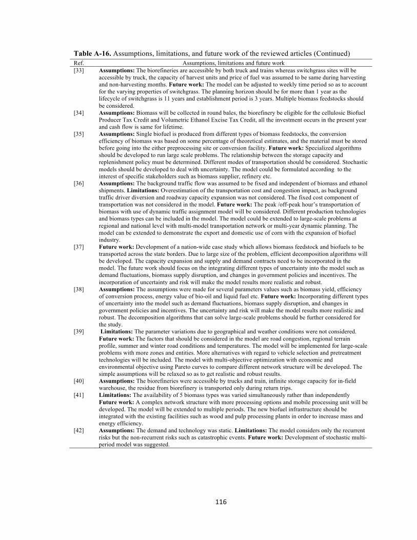
116

Table A-16. Assumptions, limitations, and future work of the reviewed articles (Continued) Ref. Assumptions, limitations and future work [33] Assumptions: The biorefineries are accessible by both truck and trains whereas switchgrass sites will be

accessible by truck, the capacity of harvest units and price of fuel was assumed to be same during harvesting and non-harvesting months. Future work: The model can be adjusted to weekly time period so as to account for the varying properties of switchgrass. The planning horizon should be for more than 1 year as the lifecycle of switchgrass is 11 years and establishment period is 3 years. Multiple biomass feedstocks should be considered.

[34] Assumptions: Biomass will be collected in round bales, the biorefinery be eligible for the cellulosic Biofuel Producer Tax Credit and Volumetric Ethanol Excise Tax Credit, all the investment occurs in the present year and cash flow is same for lifetime.

[35] Assumptions: Single biofuel is produced from different types of biomass feedstocks, the conversion efficiency of biomass was based on some percentage of theoretical estimates, and the material must be stored before going into the either preprocessing site or conversion facility. Future work: Specialized algorithms should be developed to run large scale problems. The relationship between the storage capacity and replenishment policy must be determined. Different modes of transportation should be considered. Stochastic models should be developed to deal with uncertainty. The model could be formulated according to the interest of specific stakeholders such as biomass supplier, refinery etc.

[36] Assumptions: The background traffic flow was assumed to be fixed and independent of biomass and ethanol shipments. Limitations: Overestimation of the transportation cost and congestion impact, as background traffic driver diversion and roadway capacity expansion was not considered. The fixed cost component of transportation was not considered in the model. Future work: The peak /off-peak hour’s transportation of biomass with use of dynamic traffic assignment model will be considered. Different production technologies and biomass types can be included in the model. The model could be extended to large-scale problems at regional and national level with multi-model transportation network or multi-year dynamic planning. The model can be extended to demonstrate the export and domestic use of corn with the expansion of biofuel industry.

[37] Future work: Development of a nation-wide case study which allows biomass feedstock and biofuels to be transported across the state borders. Due to large size of the problem, efficient decomposition algorithms will be developed. The capacity expansion and supply and demand contracts need to be incorporated in the model. The future work should focus on the integrating different types of uncertainty into the model such as demand fluctuations, biomass supply disruption, and changes in government policies and incentives. The incorporation of uncertainty and risk will make the model results more realistic and robust.

[38] Assumptions: The assumptions were made for several parameters values such as biomass yield, efficiency of conversion process, energy value of bio-oil and liquid fuel etc. Future work: Incorporating different types of uncertainty into the model such as demand fluctuations, biomass supply disruption, and changes in government policies and incentives. The uncertainty and risk will make the model results more realistic and robust. The decomposition algorithms that can solve large-scale problems should be further considered for the study.

[39] Limitations: The parameter variations due to geographical and weather conditions were not considered. Future work: The factors that should be considered in the model are road congestion, regional terrain profile, summer and winter road conditions and temperatures. The model will be implemented for large-scale problems with more zones and entities. More alternatives with regard to vehicle selection and pretreatment technologies will be included. The model with multi-objective optimization with economic and environmental objective using Pareto curves to compare different network structure will be developed. The simple assumptions will be relaxed so as to get realistic and robust results.

[40] Assumptions: The biorefineries were accessible by trucks and train, infinite storage capacity for in-field warehouse, the residue from biorefinery is transported only during return trips.

[41] Limitations: The availability of 5 biomass types was varied simultaneously rather than independently Future work: A complex network structure with more processing options and mobile processing unit will be developed. The model will be extended to multiple periods. The new biofuel infrastructure should be integrated with the existing facilities such as wood and pulp processing plants in order to increase mass and energy efficiency.

[42] Assumptions: The demand and technology was static. Limitations: The model considers only the recurrent risks but the non-recurrent risks such as catastrophic events. Future work: Development of stochastic multi-period model was suggested.

117

Issues, challenges and future direction

Although the numerous benefits of using biomass for bioenergy are evident in

terms of their potential to provide energy security, rural development etc., the conversion

technologies and supply logistics pose serious challenge for their commercialization [19].

The BSC is a complex system with a wide range of interconnected activities. The

upstream decisions affect the activities in the supply chain later [47]. The optimization

models help to evaluate the feasibility of biomass use for bioenergy and support decision

making at strategic, tactical and operational levels. Most of the studies reviewed focused

on location/allocation of biomass/biorefinery, inventory management and control, and

production planning. with commonly used quantitative performance measures of cost

minimization or profit maximization. The design and analysis of BSC is challenging due

to the large number of factors affecting the system. The modeling complexity increases

significantly while designing such a system. The modeling technique should consider all

the factors to provide practical solutions. (Figure A-4) [4, 43, 48, 49].

118

Figure A-4. Factor and considerations for developing modeling approach for BSC

Modeling technique and computational complexity The mixed-integer programming models (MILP) developed are capable of

making decisions related to location, technology selection, capital investment, material

and production, planning, and inventory management. These models are efficient and

effective in considering numerous factors along with providing economic, environmental

and social measures to the system [38]. But, the uncertainty in BSC is not addressed by

the MILP models. Uncertainty exists when there are chances that results will deviate

from the expected. The existence of uncertainty is associated with risk [50]. In supply

chain design, uncertainty is the major factor that influences effectiveness of configuration

119

and coordination of the supply chain system [51]. The uncertainty propagates in the

spatial and temporal dimensions of BSC, thus significantly affecting the performance of

the system. Considering uncertainty in BSC modeling is one of the major challenges

faced by researchers. The uncertainties in BSC is due to the following factors

• Biomass supply

• Weather

• Biomass properties such as moisture content

• Biomass cost

• Technology

• Expansion plans

• Demand fluctuations

• Biofuel price

• Change of Government incentives

• Change of regulations and policies

• Natural or human disasters

As uncertainty forms a major part of the problems associated with BSC modeling, a

different modeling strategy is required. Under uncertainty, the values of parameters vary

according to the nature of uncertain factors. This results in possible scenarios for the

parameters [50]. The commonly used approach to deal with uncertainty is analysis to

present scenarios separately. This technique is called the “Wait-and-see” approach, as

one has to wait and see the actual random event and make decisions according to that

situation [42]. This technique is appropriate if one scenario is analyzed, but with several

realizations or scenarios for the parameters, this technique is not appropriate. This

120

technique is appropriate if one scenario is analyzed but with several realizations or

scenarios for the parameters, this technique is not appropriate. Three other techniques to

deal with uncertainty are

• Scenario optimization

• Robust optimization

• Simulation optimization

Scenario optimization and robust optimization are the traditional methods to deal with

uncertainty. They are effective in finding feasible solution for all scenarios under

consideration. Therefore, scenario optimization technique was used for the present study.

121

References [1] Stadtler H. Supply chain management and advanced planning--basics, overview

and challenges. European Journal of Operational Research. 2005;163(3):575-588. [2] Iakovou E, Karagiannidis A, Vlachos D, Toka A, Malamakis A. Waste biomass-

to-energy supply chain management: A critical synthesis. Waste Management. 2010;30(10):1860-1870.

[3] Eksioglu SD, Acharya A, Leightley LE, Arora S. Analyzing the design and management of biomass-to-biorefinery supply chain. Computers and Industrial Engineering 2009;57(4):1342-1352.


[5] Awudu I, Zhang J. Uncertainties and sustainability concepts in biofuel supply chain management: A review. Renewable and Sustainable Energy Reviews. 2012;16(2):1359-1368.

[6] Beamon BM. Performance analysis of conjoined supply chains. International Journal of Production Research 2001;39(14):3195-3218.

[7] Min H, Zhou G. Supply chain modeling: past, present and future. Computers & Industrial Engineering. 2002;43(1-2):231-249.

[8] Mula J, Peidro D, Díaz-Madroñero M, Vicens E. Mathematical programming models for supply chain production and transport planning. European Journal of Operational Research. 2010;204(3):377-390.

[9] Keramati A, Eldabi T. Supply chain integration: Modelling approach presented at the European, Mediterranean & Middle Eastern Conference on Information Systems, Athens, Greece, 2011.

[10] Min H, Zhou G. Suppy chain modeling: Past, present and future. Computers and Industrial Engineering. 2002;43:231-249.

[11] Beamon BM. Supply chain design and analysis:: Models and methods. International Journal of Production Economics. 1998;55(3):281-294.

[12] De-Mol RM, Jogems MAH, Beek PV, Gigler JK. Simulation and optimization of the logistics of biomass fuel collection. Netherlands Journal of Agricultural Science. 1997;45


[14] Nagel J. Determination of an economic energy supply structure based on biomass using a mixed-integer linear optimization model. Ecological Engineering. 2000 16:S91–S102.


[16] Tatsiopoulos IP, Tolis AJ. Economic aspects of the cotton-stalk biomass logistics and comparison of supply chain methods. Biomass and Bioenergy. 2003;24(3):199-214.

[17] Freppaz D, Minciardi R, Robba M, Rovatti M, Sacile R, Taramasso A. Optimizing forest biomass exploitation for energy supply at a regional level. Biomass and Bioenergy. 2004;26(1):15-25.

122

[18] Gunnarsson H, Rönnqvist M, Lundgren JT. Supply chain modelling of forest fuel. European Journal of Operational Research. 2004;158(1):103-123.

[19] Morrow WR, Griffin WM, Matthews HS. Modeling Switchgrass Derived Cellulosic Ethanol Distribution in the United States. Environmental Science & Technology. 2006;40(9):2877-2886.

[20] Mapemba LD, Epplin FM, Taliaferro CM, Huhnke RL. Biorefinery feedstock production on Conservation Reserve Program land. Review of Agricultural Economics. 2007;29(2):227-246.

[21] Dunnett A, Adjiman C, Shah N. Biomass to heat supply chains applications of process optimization. Process Safety and Environmental Protection. 2007;85(5):419-429.

[22] Mapemba LD, Epplin FM, Huhnke RL, Taliaferro CM. Herbaceous plant biomass harvest and delivery cost with harvest segmented by month and number of harvest machines endogenously determined. Biomass and Bioenergy. 2008;32(11):1016-1027.

[23] D. Vlachos EI, A. Karagiannidis, A. Toka. A strategic supply chain management model for waste biomass networks. Proceedings of the 3rd International Conference on Manufacturing Engineering Chalkidiki, Greece, 2008. pp. 797-804.

[24] Frombo F, Minciardi R, Robba M, Sacile R. A decision support system for planning biomass-based energy production. Energy. 2009;34(3):362-369.

[25] Zamboni A, Shah N, Bezzo F. Spatially explicit static model for the strategic design of future bioethanol production systems. 1. Cost minimization. Energy and Fuels. 2009;23(10):5121-5133.

[26] Rentizelas AA, Tatsiopoulos IP, Tolis A. An optimization model for multi-biomass tri-generation energy supply. Biomass and Bioenergy. 2009;33(2):223-233.

[27] Yu Y, Bartle J, Li C-Z, Wu H. Mallee biomass as a key bioenergy source in Western Australia: Importance of biomass supply chain. Energy and Fuels. 2009;23(6):3290-3299.

[28] Huang Y, Chen C-W, Fan Y. Multistage optimization of the supply chains of biofuels. Transportation Research Part E: Logistics and Transportation Review. 2010;46(6):820-830.

[29] Papapostolou C, Kondili E, Kaldellis JK. Modelling biomass and biofuels supply chains, in Computer Aided Chemical Engineering. vol. Volume 29, M. C. G. E.N. Pistikopoulos ,A. C. Kokossis, Eds., ed: Elsevier, 2011, pp. 1773-1777.

[30] Akgul O, Zamboni A, Bezzo F, Shah N, Papageorgiou LG. Optimization-Based Approaches for Bioethanol Supply Chains. Industrial and Engineering Chemistry Research. 2010;50(9):4927-4938.

[31] Kim J, Realff MJ, Lee JH. Simultaneous design and operation decisions for biorefinery supply chain networks: centralized vs. distributed System. 9th International Symposium on Dynamics and Control of Process Systems, Leuven, Belgium, 2010

[32] Dal-Mas M, Giarola S, Zamboni A, Bezzo F. Strategic design and investment capacity planning of the ethanol supply chain under price uncertainty. Biomass and Bioenergy. 2011;35(5):2059-2071.

123


[34] Marvin WA, Schmidt LD, Benjaafar S, Tiffany DG, Daoutidis P. Economic optimization of a lignocellulosic biomass-to-ethanol supply chain in the Midwest Chemical Engineering Science. 2011;

[35] An H, Wilhelm WE, Searcy SW. A mathematical model to design a lignocellulosic biofuel supply chain system with a case study based on a region in Central Texas. Bioresource Technology. 2011;102:7860-7870.

[36] Bai Y, Hwang T, Kang S, Ouyang Y. Biofuel refinery location and supply chain planning under traffic congestion. Transportation Research Part B: Methodological. 2011;45(1):162-175.

[37] You F, Tao L, Graziano DJ, Snyder SW. Optimal design of sustainable cellulosic biofuel supply chains: Multiobjective optimization coupled with life cycle assessment and input–output analysis. American Institute of Chemical Engineers. 2011;

[38] You F, Wang B. Life cycle optimization of biomass-to-liquids supply chains with distributed-centralized processing networks. Industrial & Engineering Chemistry Research. 2011:null-null.

[39] Lam HL, Klemeš JJ, Kravanja Z. Model-size reduction techniques for large-scale biomass production and supply networks. Energy. 2011;36(8):4599-4608.

[40] Zhu X, Yao Q. Logistics system design for biomass-to-bioenergy industry with multiple types of feedstocks. Bioresource Technology. 2011;102(23):10936-10945.

[41] Kim J, Realff MJ, Lee JH. Optimal design and global sensitivity analysis of biomass supply chain networks for biofuels under uncertainty. Computers and Chemical Engineering. 2011;35:1738-1751.

[42] Chen C-W, Fan Y. Bioethanol Supply Chain System Planning under Supply and Demand Uncertainties. Transportation Research Part E 2011;48(1):150-164.

[43] Rentizelas AA, Tolis AJ, Tatsiopoulos IP. Logistics issues of biomass: The storage problem and the multi-biomass supply chain. Renewable and Sustainable Energy Reviews. 2009;13(4):887-894.

[44] Stair RM, Reynolds G, Reynolds GW. Principles of Information Systems. [45] Cogeneration. c2012 [cited 2012 Feb 1 ]. Available from:

http://en.wikipedia.org/wiki/Anonymous_(group). [46] DOE. CHP fuels; c2012 [cited 2012 February 1]. Available from:

http://www.gulfcoastcleanenergy.org/CLEANENERGY/CombinedHeatandPower/Fuels/tabid/1790/Default.aspx.

[47] Allen J, Browne M, Hunter A, Boyd J, Palmer H. Logistics management and costs of biomass fuel supply. International Journal of Physical Distribution & Logistics Management. 1998;28(6):463 - 477.

[48] Gold S, Seuring S. Supply chain and logistics issues of bio-energy production. Journal of Cleaner Production. 2011;19(1):32-42.

[49] IEA. International Energy Agency: Good practice guidelines: bioenergy project development & biomass supply. Organization for Economic Co-operation and Development (OECD), Paris, France;2007.

124


[51] Peidro D, Mula J, Poler R, Lario F-C. Quantitative models for supply chain planning under uncertainty: a review. The International Journal of Advanced Manufacturing Technology. 2009;43(3):400-420.

125

APPENDIX-B

126

Model formulation A scenario optimization model was developed to minimize the total cost of the

system throughout the one year planning horizon.

Table B-1. Model indices and descriptions Index Description

Main set I Set of harvesting sites: i={So-1,So-2, So-3,So-4, So-5,So-6,

So-7} J Set of inventory sites: j={Inv-1, Inv-2, Inv-3, Inv-4, Inv-5} S Set of storage treatments: s={GT,TP,UP} T Set of time periods: t={TP-1,TP-2, TP-3,TP-4, TP-5,TP-6,

TP-7,TP-8} W Set of weather scenarios: w={WS-1,WS-2, WS-3,WS-4, WS-

5,WS-6, WS-7,WS-8, WS-9,WS-10, WS-11,WS-12} l Set of land categories

127

Table B-2. List of parameters used in the model Parameters Description DENt Demand of biomass in a time period t (ton) CPROC Cost of procuring switchgrass ($/ton) PWSw Probability of weather scenario w (fraction) PROC Processing cost of biomass feedstock in biorefinery ($/gallon) BFtw Before-frost time period t in weather scenario w (fraction) STORCs Storage cost of biomass for storage method ($/ton) VCTUSIij Variable cost of transporting biomass from source county i to inventory site j

($/ton) VCTUSBi Variable cost of transporting biomass from source county i to biorefinery site

($/ton) VCTUIBj Variable cost of transporting biomass from inventory site j to biorefinery site

($/ton) VCHUBF Variable cost of harvesting unit before frost ($/acre) VCHUAF Variable cost of harvesting unit after frost ($/acre) FCHUBF Annual fixed cost of harvest unit before frost ($/year) FCHUAF Annual fixed cost of harvest unit after frost ($/year) VCTUL Variable cost of in-field transportation unit ($/ton) FCTUL Fixed cost of in-field transportation unit ($/year) FCTU Fixed cost of transportation unit ($/year) ACRELANDli Acres of land at source site i under land category l (acres) PROPil Proportion of land category l at biomass source site i suitable for cultivation

of biomass (fraction) YADJt Yield adjustment factor for time period t (vary between 0 to 1) YIELDl Yield of biomass for land category l (tons/acre) CAPHUBF Capacity of harvest unit before frost (acres/hr.) CAPHUAF Capacity of harvest unit after frost (acres/hr.) WDHtw Number of harvesting work hours available in a time period t and weather

scenario w (hrs.) CAPTUL Capacity of in-field transportation unit (tons/hr.) CAPINVj Capacity of inventory site j (tons) CAPSTOR Capacity of storage site (tons) CAPTU Capacity of transportation unit (tons/load) DMLOSSs Dry matter loss for storage method s INVSTART Inventory at beginning of the weather scenario (tons) INVEND Inventory at end of the weather scenario (tons) COSTFL Cost of biomass sold to outside source ($/ton) COSTDEMSUPP Cost of biomass supply from outside source to fill the safety stock ($/ton) COSTINVSUPP Cost of biomass supply from outside source to fill inventory ($/ton) CRHUBF Rental rate for the harvest unit before frost ($/day) CRHUBF Rental rate for the harvest unit after frost ($/day) CRNPTUL Rental rate for the infield transportation units ($/day)

128

Table B-3. List of variables used for the model Variables Description sabfitlw Acres of biomass harvested from land category l in source county i in time period t before-

frost under weather scenario w saafitlw Acres of biomass harvested from land category l in source county i in time period t after

frost under weather scenario w tbfitlw Tons of biomass harvested from source county i in time period t from land category l before

frost under weather scenario w tafitlw Tons of biomass harvested from source county i in time period t from land category l after

frost under weather scenario w stiistw Tons of biomass stored at inventory site j under storage treatment s in time period t and

weather scenario w tssiijtw Tons of biomass transported from source county i to inventory site j in time period t and

weather scenario w tssbitw Tons of biomass transported from source county i to biorefinery site in time period t and

weather scenario w tsibjtw Tons of biomass transported from inventory site j to biorefinery site in time period t and

weather scenario w hubf Total number of harvest units before frost huaf Total number of harvest units after frost ahuaf Number of additional harvest units after frost ntul Total number of in-field transport units nhubfaitw Total harvest units before frost allocated to source site i in a time period t and weather

scenario w nhuafaitw Total harvest units after frost allocated to source site i in time period t and weather scenario

w nptulitw Total in-field transportation units allocated to site county i in time period t and weather

scenario w ntul Number of in-field transportation units tasijstw Tons of biomass transported from source site to inventory site j allocated to different storage

treatments s in time period t and weather scenario w ttisjstw Tons of biomass transported from inventory site j to biorefinery site allocated to different

storage treatments s in time period t and weather scenario w ntu Number of transport units undemandtw Tons of unmet demand in time period t under weather scenario w nstor Number of storage units outdemsup Demand met from outside supply nptulitw Harvest units purchased in-field transportation units allocated to source site i in a time

period t and weather scenario w rnhubfaitw Rented harvest units before frost allocated to source site i in a time period t and weather

scenario w rnhuafaitw Rented harvest units after frost allocated to source site i in a time period t and weather

scenario w tsfl Tons of biomass sold to feedlot acrelease Total acrealesed for biomass production renptulitw Rented in-field transportation units allocated to source site i in a time period t and weather

scenario w nphuafaitw Purchased harvest units after frost allocated to source site i in a time period t and weather

scenario w nphubfaitw Purchased harvest units before frost allocated to source site i in a time period t and weather

scenario w nrhubfaitw Rented harvest units before frost allocated to source site i in a time period t and weather

scenario w nrhuafaitw Rented harvest units after frost allocated to source site i in a time period t and weather

scenario w

129

The following equations present the minimization objective function for the model.

The total cost for the biorefinery has the following components described in appendix 1

• Biomass procuring cost(Cbp) • Cost of acres leased (Cal) • Fixed cost (Cfctt) and variable cost (Cvctt) of transportation • Fixed cost (Cfchu) and variable cost (Cvchu) of harvest units • Fixed cost (Cfciftu) and variable cost (Cvciftu) of in-field transportation units • Variable cost (Crchu) of rented harvest units • Fixed cost (Cfciftu) and variable cost (Cvciftu) of in-field transportation units

Biomass procuring cost (Cbp):

C!" = tbf!"#$

!

!!!

!

!!!

!

!!!

!

!!!

×CTON×BF!" × PWS!

+ taf!"#$

!

!!!

!

!!!

!

!!!

!

!!!

×CTON× 1 − BF!" ×PWS!

Cost of acres leased:

C!"= acrelease!"

W

w=1

L

l=1

I

s=1

×COSTACREil×PWSw

Fixed cost (Cfctt) and variable cost (Cvctt) of transportation:

Cfctt=FCTU×ntu

Ctt= tssiijtw×W

w=1

VCTUSIij×PWSw

T

t=1

J

j=1

I

i=1

+ tssbitw

W

w=1

×VCTUSBi×PWSw

T

t=1

I

i=1

+

tsibjtw

W

w=1

×VCTUIBj×PWSw T

t=1

J

j=1

130

Fixed cost (Cfchu) and variable cost (Cvchu) of harvest units:

Cfchu= FCHUBF×hubf + FCHUAF×ahuaf

Cvchu= sabfitlw×W

w=1

L

l=1

T

t=1

I

i=1

VCHUBF× BFtw×PWSw + saafitlw×W

w=1

L

l=1

T

t=1

I

i=1

VCHUAF × 1-BFtw ×PWSw

Fixed cost (Cfciftu) and variable cost (Cvciftu) of in-field transportation units:

C!"#!$% = FCTUL × NTUL

Cvciftu= tbfitlw

W

w=1

L

l=1

T

t=1

I

i=1

×VCTUL×BFtw×PWSw + tafitlw

W

w=1

L

l=1

T

t=1

I

i=1

×VCTUL× 1-BFtw ×PWSw

Variable cost (Crchu) of rented harvest units

Crchu= rnhubfa!"#

W

w=1

T

t=1

I

i=1

×CRHUBF×WDAYtw×BFtw×PWSw

+ rnhuafa!"#

W

w=1

T

t=1

I

i=1

×CRHUBF×WDAY!"× 1-BFtw ×PWSw

Variable cost (Crifhu) of rented in-field transportation units units

Crifhu= renptul!"#

W

w=1

T

t=1

I

i=1

×CRNPTUL×PWSw

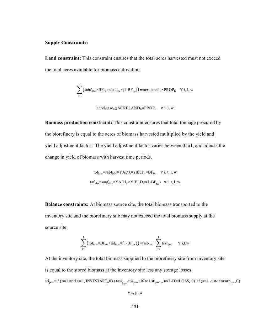
131

Supply Constraints:

Land constraint: This constraint ensures that the total acres harvested must not exceed

the total acres available for biomass cultivation.

sabfitlw×BFtw+saafitlw×(1-BFtw)T

t=1

=acreleaseli×PROPli ∀ i, l, w

acreleaseli≤ACRELANDli×PROPli ∀ i, l, w

Biomass production constraint: This constraint ensures that total tonnage procured by

the biorefinery is equal to the acres of biomass harvested multiplied by the yield and

yield adjustment factor. The yield adjustment factor varies between 0 to1, and adjusts the

change in yield of biomass with harvest time periods.

tbfitlw=sabfitlw×YADJt×YIELD!×BFtw ∀ i, t, l, w

tafitlw=saafitlw×YADJt ×YIELDl×(1-BFtw) ∀ i, t, l, w

Balance constraints: At biomass source site, the total biomass transported to the

inventory site and the biorefinery site may not exceed the total biomass supply at the

source site

tbfitlw×BFtw+tafitlw× 1-BFtw

L

l=1

=tssbitw+ tssiijtw

J

j=1

∀ i,t,w

At the inventory site, the total biomass supplied to the biorefinery site from inventory site

is equal to the stored biomass at the inventory site less any storage losses.

stijstw=if (t=1 and s=1, INVTSTART! ,0)+tasijstw-ttisjstw+if(t>1,stijst-1,w)×(1-DMLOSSs,0)+if (s=1, outdemsup!"#,0)

∀ s, j,t,w

132

stij1,12,w ≥ INVEND! ∀ t,w

The following constraints allocate the biomass transported to the inventory site from

biomass source sites to different storage treatments.

tssiijtw

I

i=1

= tasijstw

S

s=1

∀ j,t,w

tsibjtw

I

i=1

= ttisjstw

S

s=1

∀ j,t

Demand constraint: At biorefinery site, the biomass transported to biorefinery site from

source site and inventory site considering the unmet demand must be equal to the demand

of biorefinery

tsibjtw+ tssbitw

I

i=1

J

j=1

+undemandtw =DENt ∀ t,w

Inventory site capacity constraint: The constraint ensures that the total biomass stored

at the inventory site may not exceed the capacity of the inventory site

stijstw

S

s=1

≤CAPINVj ∀ j,t, w

Harvest unit: The total number of harvest units after frost is equal to number of harvest

units used during the before frost period along with additional units required to handle the

heavier demands of added acreage for after frost harvesting.

huaf = hubf + ahuaf

The following constraint ensures that the biomass acres harvested may not exceed the

combined capacity of harvest units allocated to the biomass source sites. The constraints

133

also consider the work hours hours available for harvesting biomass in a weather scenario

and time period.

sabfitlw

L

l=1

×BFtw+saafitlw×(1-BFtw)≤ nhubfaitw×CAPHUBF×BFtw+nhuafaitw×CAPHUAF × (1-BFtw) ×WDHtw∀ i, t, w

tbfitlw×BFtw+tafitlw× 1-BFtw ≤ nptul!"#×CAPTUL×WDH!" ∀ i,t,w

nhubfaitw = nphubfa!"# + rnhubfa!"# ∀ i,t,w

nhuafaitw = nphuafa!"# + rnhuafa!"# ∀ i,t,w

nptulitw = npurtul!"# + renptul!"# ∀ i,t,w

The next constraint ensures that the sum of the harvest units may not exceed the total

number of harvest units determined by the model

nphubfaitw

!

!!!

=hubf×BFtw ∀ t,w

nphuafaitw

!

!!!

=hubf× 1-‐BFtw ∀ t,w

The sum of the in-field transportation units may not exceed the combined capacity of in-

field transportation units endogenously determined by the model

npurtul!

!!!

=ntul ∀ t,w

Transportation unit: The constraint ensures that the biomass tons transported from

source site to inventory site, inventory site to biorefinery and source site to biorefinery

may not exceed the total number of transportation units

tssiijtw

J

j=1

I

i=1

+ tssbitw

I

i=1

+ tsibjtw

J

j=1

≤CAPTU×ntu ∀ t,w

134

Logical Constraints: The other constraints are the logical constraints or non-negativity

constraints on variables. The integer constraints were on variables: hubf, huaf, ahuaf, ntul

, ntu , nhubfaitw , nhuafaitw , nphubfaitw, nphuafaitw, nrhuafaitw, nrhubfaitw, and nptulitw..

135

APPENDIX-C

.

136

Table C-1. Summary of weather parameters for all harvesting months in a weather scenario

Weather Scenario

Days for which FWI values>0.8

Minimum temperature (F)

Solar radiation (MJ/m2)

Total rain (inches)

1998-1999 46 -3.68 4014 15.9 1999-2000 1 8.83 4031 4.11 2000-2001 22 3.61 3974 8.95 2001-2002 4 3.67 4001 4.19 2002-2003 33 1.11 3803 10.94 2003-2004 2 -2.74 3859 5.75 2004-2005 58 -11.85 3538 13.94 2005-2006 2 -8.34 3937 6.35 2006-2007 34 -4.22 3810 14.11 2007-2008 6 -0.09 4043 4.01 2008-2009 28 3.79 3867 15.13 2009-2010 33 -5.85 3774 9.98

137

Table C-2. Fixed and variable cost calculation for self-propelled windrower Machine Self-propelled Windrower hp requirement 190 Cutting width (ft.) 16 Efficiency (%) 80 Speed (mph) 8 Effective field capacity (acres/hr.) 12.4 Yield (tons/acre) 2 Annual ownership cost

List Price ($) 149309 Purchase price (fraction) of list price 0.85 Purchase price ($) 126913 Useful life (hr.) 3000 Total harvest hours per year (hours/year) 1612 Useful life (year) 1.861042184 Interest rate (%) 0.07 C1 0.7557 C2 0.0672 C3 0 RV (%) 44.1 RV (Dec.) 0.4 Salvage value ($) (trade in value) 65834.8 Rates of taxes, housing, insurance (%) 0.02 Insurance, taxes, housing ($) 1927.47 Annual fixed cost ($/year) 47196.34034 Repair & Maintenance cost

Crm_life (Total life R & M cost (% of list price) 0.55 Repair and maintenance ($/hr.) 27.37331667 Fuel & lubrication cost

Typical fuel use for a specific operation (gal/hp/hr.) 0.08 Fuel use (Gallon/hr.) 11.12 Diesel price ($/gallon) 3.8 Fuel cost ($/hr.) 42.25 Lube & oil (% of fuel cost) 15 Cost of lube and oil ($/hr.) 6.34 Labor Cost

Labor rate ($/hr.) 11.2 Factor-1 (Fringe benefits of 30% ) 1.3 Factor-2 (20% additional labor over the amount of time an implement operates) 1.2 Total labor cost ($/hr.) 17.5 Total VC ($/hr.) 93.4 Total FC($/Year) 47196.3

VITA

Bhavna Sharma

Candidate for the Degree of

Doctor of Philosophy Thesis: SCENARIO OPTIMIZATION APPROACH FOR DESIGNING BIOMASS SUPPLY CHAIN Major Field: Biosystems and Agricultural Engineering Biographical:

Education: Completed the requirements for the Doctor of Philosophy/Education in your major at Oklahoma State University, Stillwater, Oklahoma in December, 2012. Completed the requirements for the Master of Science in Industrial Engineering and Management, Oklahoma State University Stillwater, Okalhoma, 2012. Completed the requirements for the Master of Science in Processing and Food Engineering , Punjab Agricultural University, Ludhiana, Punjab, India in 2007. Completed the requirements for the Bachelor of Science in Food Technology, Sant Longowal Institute of Engineering and Technology, Longowal, Punjab, India in 2004. Experience: Shift-Incharge, Thakur Mushroom, Solan, Himachal Pradesh, India August 2004-July 2005

Professional Memberships: Member, APICS The Association for Operations

Management , 2012. Member, Institute of Operations Research and Management Science, 2011-Present, Member, American Society of Agricultural and Biological Engineer, 2007-Present

ADVISER’S APPROVAL: Dr. Carol L. Jones

Name: Bhavna Sharma Date of Degree: December, 2012 Institution: Oklahoma State University Location: Stillwater, Oklahoma Title of Study: SCENARIO OPTIMIZATION APPROACH FOR DESIGNING BIOMASS SUPPLY CHAIN Pages in Study: 137 Candidate for the Degree of Doctor of Philosophy

Major Field: Biosystems and Agricultural Engineering Scope and Method of Study:

Commercialization of biofuel industry is highly dependent on development of efficient biomass supply chain system. The effect of uncertain parameters on biomass supply chain needs to be investigated for realistic and robust economic assessment of the system. The present study focuses on the development of scenario optimization model for minimizing cost of biomass supply to biorefinery under weather uncertainty. The model determines material flow, number of harvest units, in-field transportation units, transportation units, storage method, and allocation of units to sites. The applicability of proposed model is demonstrated by developing a case study for Abengoa ethanol biorefinery at Hugoton, Kansas. Findings and Conclusions:

The scenario optimization model developed in the present study has the ability to determine material flows along with the number of harvesting units, in-field transportation units, and transportation units required by the biorefinery while considering the weather uncertainty. The optimization model takes into consideration the purchasing and deployment of assets, with a highly seasonal production of biomass. The case study for Abengoa Biorefinery at Hugoton, Kansas presents the practical application of the model. It was concluded that harvest work hours influence the major cost related decisions in biomass supply chain. The results also indicate that yield of biomass is a crucial factor in determining the profit of biomass supply to the biorefinery. The modeling approach can be also extended to large-scale application. The direction for future research should be to consider different types of biomass feedstocks and conversion processes into the model.