department of agricultural economics – - resource...

Basic LP formulationsLinear programming formulations are typically composed

of a number of standard problem types.

In these notes we review four basic problems examining

their:

a. Basic Structure

b. Formulation

c. Example application

d. Answer interpretation

The problems examined are the:

a. Resource allocation problem

b. Transportation problem

c. Feed mix problem

d. Joint products problem

CH 05-OH-1

Resource Allocation ProblemBasic Concept

The classical LP problem involves the allocation of an

endowment of scarce resources among a number of

competing products so as to maximize profits.

Objective: Maximize Profits

Indexes: Let the competing products index be jLet the scarce resources index be i

Variables: Let us define our primary decision variable Xj, as the number of units of the jth product made

Restrictions: Non negative production Resource usage across all production possibilities is less than or equal to the resource endowment

CH 05-OH-2

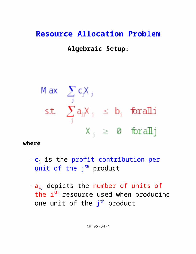
Resource Allocation ProblemAlgebraic Setup:

where

- cj is the profit contribution per unit of the jth product

- aij depicts the number of units of the ith resource used when producing one unit of the jth product

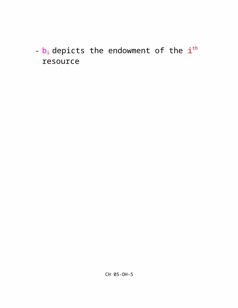
- bi depicts the endowment of the ith resource

CH 05-OH-3

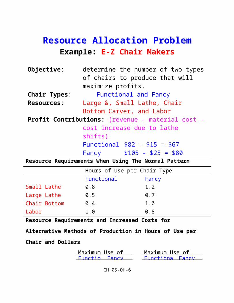
Resource Allocation ProblemExample: E-Z Chair Makers

Objective: determine the number of two types of chairs to produce that will maximize profits.

Chair Types: Functional and FancyResources: Large &, Small Lathe, Chair Bottom Carver, and

LaborProfit Contributions: (revenue – material cost - cost increase due to

lathe shifts)Functional $82 - $15 = $67Fancy $105 - $25 = $80

Resource Requirements When Using The Normal Pattern

Hours of Use per Chair TypeFunctional Fancy

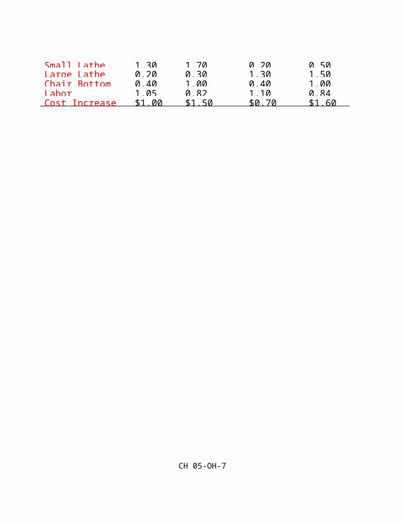
Small Lathe 0.8 1.2Large Lathe 0.5 0.7Chair Bottom Carver 0.4 1.0Labor 1.0 0.8Resource Requirements and Increased Costs for Alternative Methods of

Production in Hours of Use per Chair and Dollars

Maximum Use of Small Maximum Use of Large Functional Fancy Functional Fancy

Small Lathe 1.30 1.70 0.20 0.50Large Lathe 0.20 0.30 1.30 1.50Chair Bottom Carver 0.40 1.00 0.40 1.00Labor 1.05 0.82 1.10 0.84Cost Increase $1.00 $1.50 $0.70 $1.60

CH 05-OH-4

Resource Allocation ProblemExample: E-Z Chair Makers

Algebraic Setup:

Empirical Setup:

Max 67X1 + 66X2 + 66.3X3 + 80X4 + 78.5X5 + 78.4X6

s.t. 0.8X1 + 1.3X2 + 0.2X3 + 1.2X4 + 1.7X5 + 0.5X6 ≤ 140

0.5X1 + 0.2X2 + 1.3X3 + 0.7X4 + 0.3X5 + 1.5X6 ≤ 90

0.4X1 + 0.4X2 + 0.4X3 + X4 + X5 + X6 ≤ 120

X1 + 1.05X2 + 1.1X3 + 0.8X4 + 0.82X5 + 0.84X6 ≤ 125

X1 , X2 , X3 , X4 , X5 , X6 ≥ 0

Where:X1 = the # of functional chairs made with the normal pattern;X2 = the # of functional chairs made with maximum use of the small lathe;X3 = the # of functional chairs made with maximum use of the large lathe;X4 = the # of fancy chairs made with the normal pattern;X5 = the # of fancy chairs made with maximum use of the small lathe;X6 = the # of fancy chairs made with maximum use of the large lathe.

CH 05-OH-5

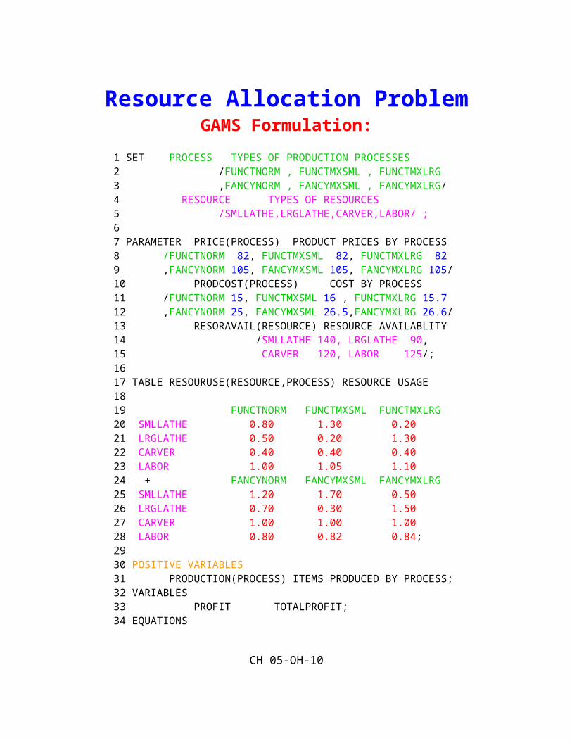
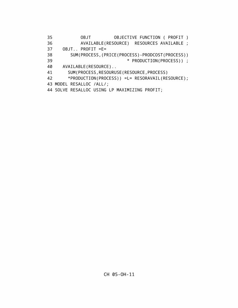
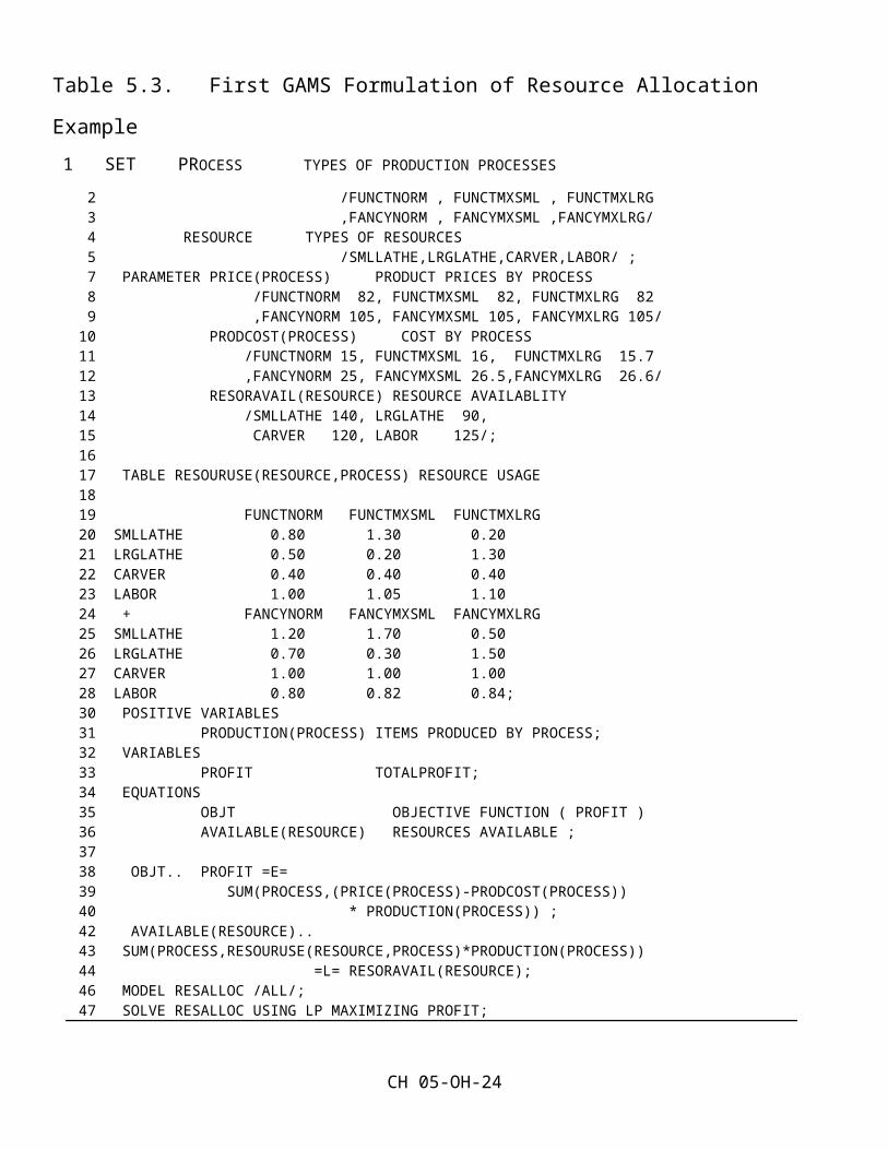
Resource Allocation ProblemGAMS Formulation:

1 SET PROCESS TYPES OF PRODUCTION PROCESSES 2 /FUNCTNORM , FUNCTMXSML , FUNCTMXLRG 3 ,FANCYNORM , FANCYMXSML , FANCYMXLRG/ 4 RESOURCE TYPES OF RESOURCES 5 /SMLLATHE,LRGLATHE,CARVER,LABOR/ ; 6 7 PARAMETER PRICE(PROCESS) PRODUCT PRICES BY PROCESS 8 /FUNCTNORM 82, FUNCTMXSML 82, FUNCTMXLRG 82 9 ,FANCYNORM 105, FANCYMXSML 105, FANCYMXLRG 105/ 10 PRODCOST(PROCESS) COST BY PROCESS 11 /FUNCTNORM 15, FUNCTMXSML 16 , FUNCTMXLRG 15.7 12 ,FANCYNORM 25, FANCYMXSML 26.5,FANCYMXLRG 26.6/ 13 RESORAVAIL(RESOURCE) RESOURCE AVAILABLITY 14 /SMLLATHE 140, LRGLATHE 90, 15 CARVER 120, LABOR 125/; 16 17 TABLE RESOURUSE(RESOURCE,PROCESS) RESOURCE USAGE 18 19 FUNCTNORM FUNCTMXSML FUNCTMXLRG 20 SMLLATHE 0.80 1.30 0.20 21 LRGLATHE 0.50 0.20 1.30 22 CARVER 0.40 0.40 0.40 23 LABOR 1.00 1.05 1.10 24 + FANCYNORM FANCYMXSML FANCYMXLRG 25 SMLLATHE 1.20 1.70 0.50 26 LRGLATHE 0.70 0.30 1.50 27 CARVER 1.00 1.00 1.00 28 LABOR 0.80 0.82 0.84; 29 30 POSITIVE VARIABLES 31 PRODUCTION(PROCESS) ITEMS PRODUCED BY PROCESS; 32 VARIABLES 33 PROFIT TOTALPROFIT; 34 EQUATIONS 35 OBJT OBJECTIVE FUNCTION ( PROFIT ) 36 AVAILABLE(RESOURCE) RESOURCES AVAILABLE ; 37 OBJT.. PROFIT =E= 38 SUM(PROCESS,(PRICE(PROCESS)-PRODCOST(PROCESS)) 39 * PRODUCTION(PROCESS)) ; 40 AVAILABLE(RESOURCE).. 41 SUM(PROCESS,RESOURUSE(RESOURCE,PROCESS) 42 *PRODUCTION(PROCESS)) =L= RESORAVAIL(RESOURCE); 43 MODEL RESALLOC /ALL/;

CH 05-OH-6

44 SOLVE RESALLOC USING LP MAXIMIZING PROFIT;

CH 05-OH-7

Resource Allocation ProblemPrimal and Solution:

Max 67X1 + 66X2 + 66.3X3 + 80X4 + 78.5X5 + 78.4X6

s.t. 0.8X1 + 1.3X2 + 0.2X3 + 1.2X4 + 1.7X5 + 0.5X6 ≤ 140

0.5X1 + 0.2X2 + 1.3X3 + 0.7X4 + 0.3X5 + 1.5X6 ≤ 90

0.4X1 + 0.4X2 + 0.4X3 + X4 + X5 + X6 ≤ 120

X1 + 1.05X2 + 1.1X3 + 0.8X4 + 0.82X5 + 0.84X6 ≤ 125

X1 , X2 , X3 , X4 , X5 , X6 ≥ 0

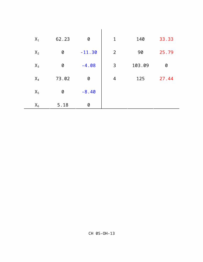
Recall:Shadow Price represents marginal values of the resourcesReduced Cost represents marginal costs of forcing non-basic variable into the solution

Table 5.5 Optimal Solution to the E-Z Chair Makers Problem

obj = 10417.29

Variables Value Reduced Cost Constraint Level Shadow Price

X1 62.23 0 1 140 33.33

X2 0 -11.30 2 90 25.79

X3 0 -4.08 3 103.09 0

X4 73.02 0 4 125 27.44

X5 0 -8.40

CH 05-OH-8

X6 5.18 0

CH 05-OH-9

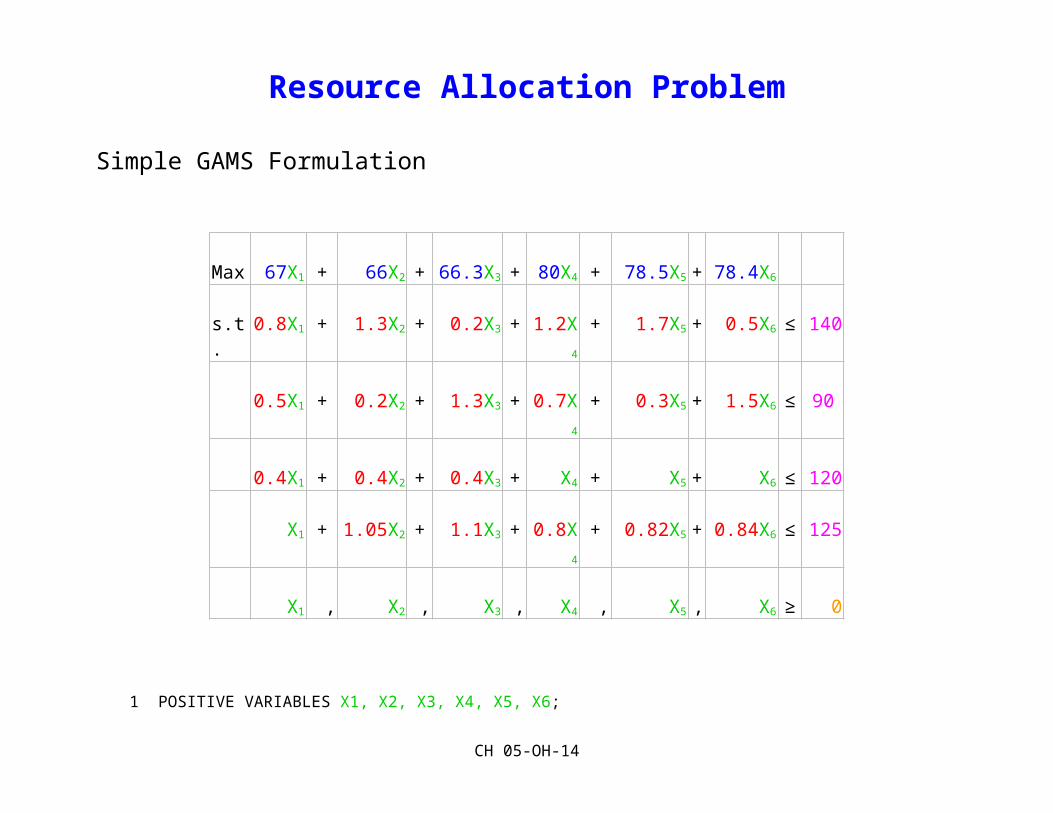
Resource Allocation Problem

Simple GAMS Formulation

Max 67X1 + 66X2 + 66.3X3 + 80X4 + 78.5X5 + 78.4X6

s.t. 0.8X1 + 1.3X2 + 0.2X3 + 1.2X4 + 1.7X5 + 0.5X6 ≤ 140

0.5X1 + 0.2X2 + 1.3X3 + 0.7X4 + 0.3X5 + 1.5X6 ≤ 90

0.4X1 + 0.4X2 + 0.4X3 + X4 + X5 + X6 ≤ 120

X1 + 1.05X2 + 1.1X3 + 0.8X4 + 0.82X5 + 0.84X6 ≤ 125

X1 , X2 , X3 , X4 , X5 , X6 ≥ 0

1 POSITIVE VARIABLES X1, X2, X3, X4, X5, X6; 2 VARIABLE PROFIT; 3 EQUATIONS OBJFUNC, CONSTR1, CONSTR2, CONSTR3, CONSTR4; 4 OBJFUNC.. 67*X1 + 66*X2 + 66.3*X3 + 80*X4 + 78.5*X5 + 78.4*X6 =E= PROFIT; 5 CONSTR1.. 0.8*X1 + 1.3*X2 + 0.2*X3 + 1.2*X4 + 1.7*X5 + 0.5*X6 =L= 140; 6 CONSTR2.. 0.5*X1 + 0.2*X2 + 1.3*X3 + 0.7*X4 + 0.3*X5 + 1.5*X6 =L= 90; 7 CONSTR3.. 0.4*X1 + 0.4*X2 + 0.4*X3 + X4 + X5 + X6 =L= 120; 8 CONSTR4.. X1 + 1.05*X2 + 1.1*X3 + 0.8*X4 + 0.82*X5 + 0.84*X6 =L= 125; 9 MODEL EXAMPLE1 /ALL/;10 SOLVE EXAMPLE1 USING LP MAXIMIZING PROFIT;

CH 05-OH-10

Resource Allocation Problem

Primal and Dual Algebra:

Primal

Max ∑jc j X j

s . t . ∑ja ijX j ¿ b i for all i

X j ¿ 0 for all j

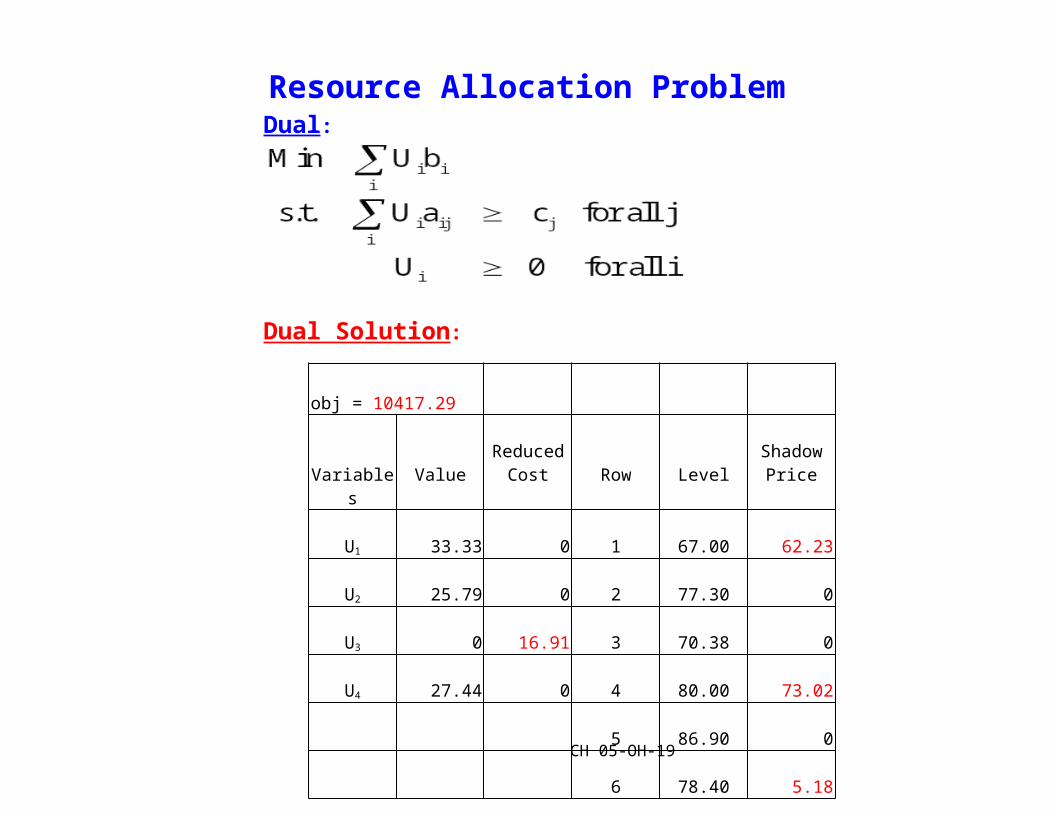
Dual

Min ∑iU ibi

s . t . ∑iU ia ij ¿ c j for all j

Ui ¿ 0 for all i

CH 05-OH-11

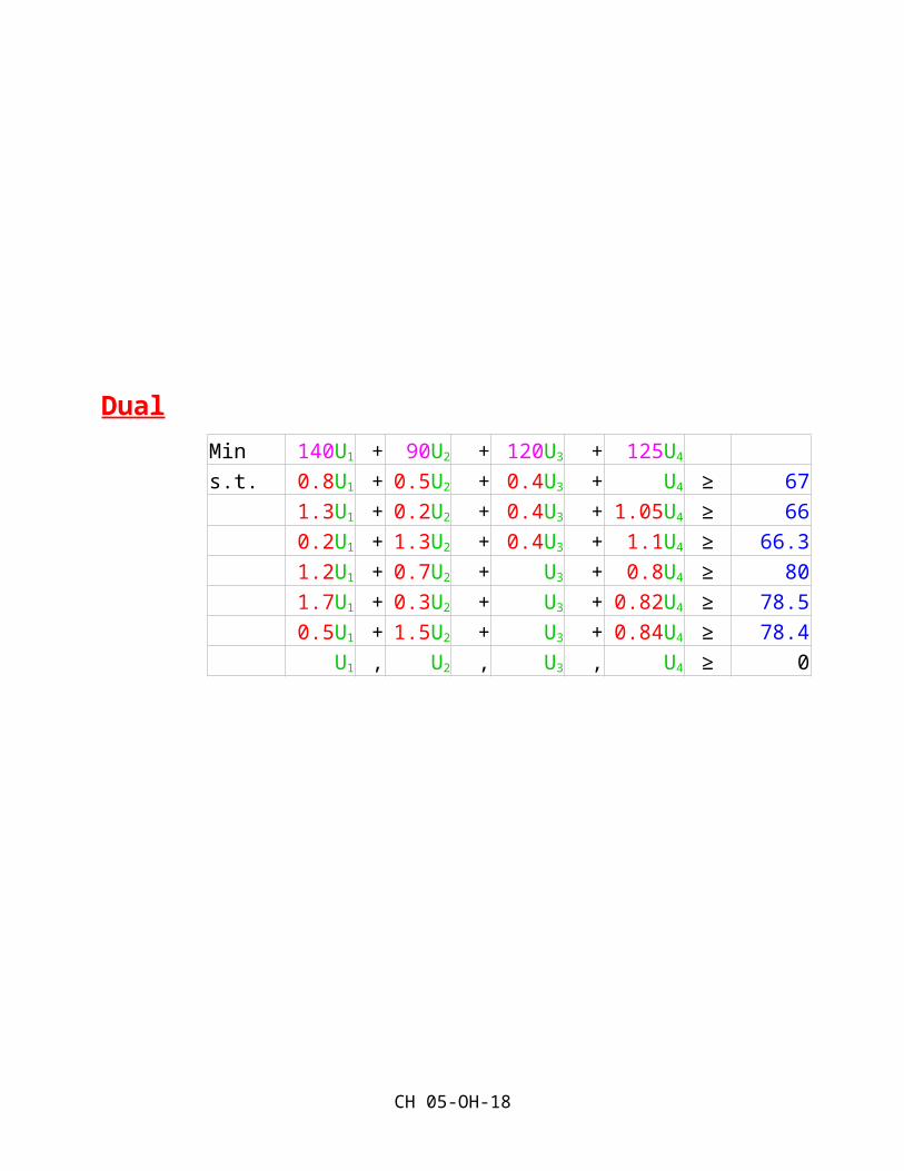
Resource Allocation ProblemPrimal and Dual Empirical:

Primal

Dual

Max 67X1 + 66X2 + 66.3X3 + 80X4 + 78.5X5 + 78.4X6

s.t. 0.8X1 + 1.3X2 + 0.2X3 + 1.2X4 + 1.7X5 + 0.5X6 ≤ 140

0.5X1 + 0.2X2 + 1.3X3 + 0.7X4 + 0.3X5 + 1.5X6 ≤ 90

0.4X1 + 0.4X2 + 0.4X3 + X4 + X5 + X6 ≤ 120

X1 + 1.05X2 + 1.1X3 + 0.8X4 + 0.82X5 + 0.84X6 ≤ 125

X1 , X2 , X3 , X4 , X5 , X6 ≥ 0

Min 140U1 + 90U2 + 120U3 + 125U4

s.t. 0.8U1 + 0.5U2 + 0.4U3 + U4 ≥ 671.3U1 + 0.2U2 + 0.4U3 + 1.05U4 ≥ 66

0.2U1 + 1.3U2 + 0.4U3 + 1.1U4 ≥ 66.3

1.2U1 + 0.7U2 + U3 + 0.8U4 ≥ 80

1.7U1 + 0.3U2 + U3 + 0.82U4 ≥ 78.5

0.5U1 + 1.5U2 + U3 + 0.84U4 ≥ 78.4

U1 , U2 , U3 , U4 ≥ 0

CH 05-OH-12

Resource Allocation ProblemDual:

Dual Solution:

obj = 10417.29

Variables ValueReduced

Cost Row LevelShadow

Price

U1 33.33 0 1 67.00 62.23

U2 25.79 0 2 77.30 0

U3 0 16.91 3 70.38 0

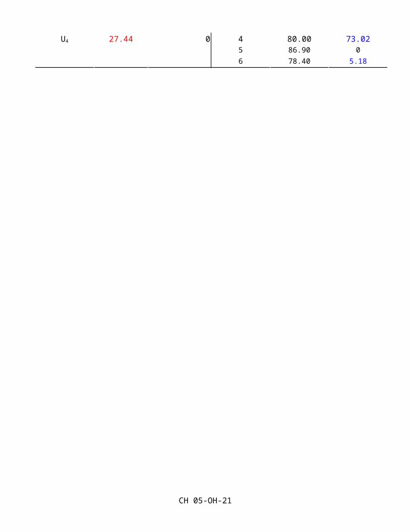
U4 27.44 0 4 80.00 73.02

5 86.90 0

6 78.40 5.18

CH 05-OH-13

Resource Allocation

Primal and Dual Solution Comparison:

Table 5.5 Optimal Solution to the E-Z Chair Makers Problem

obj = 10417.29

Variables Value Reduced Cost Constraint Level Shadow Price

X1 62.23 0 1 140 33.33

X2 0 -11.30 2 90 25.79

X3 0 -4.08 3 103.09 0

X4 73.02 0 4 125 27.44

X5 0 -8.40

X6 5.18 0

Table 5.5a Optimal Solution to the Dual E-Z Chair Makers Problem

obj = 10417.29

Variables Value Reduced Cost Constraint Level Shadow PriceU1 33.33 0 1 67.00 62.23U2 25.79 0 2 77.30 0U3 0 16.91 3 70.38 0U4 27.44 0 4 80.00 73.02

5 86.90 06 78.40 5.18

CH 05-OH-14

0.8U1 + 0.5U2 + 0.4U3 + U4 > 671.3U1 + 0.2U2 + 0.4U3 + 1.05U4 > 66

Dual SolutionU1 33.33U2 25.79U3 0U4 27.44

Evaluation0.8(33.33) + 0.5(25.79) +0.4(0) +27.44 > 6726.6664 + 12.895 + 0 +27.44 > 6767 > 67Reduced cost=0

1.3U1 + 0.2U2 + 0.4U3 + 1.05U4 > 661.3(33.33)+ 0.2(25.79) +0.4(0) +1.05(27.44) > 6643.33 + 5.16 +0 + 28.812 > 6677.3 > 6666+11.3 > 66Reduced cost=11.3

CH 05-OH-15

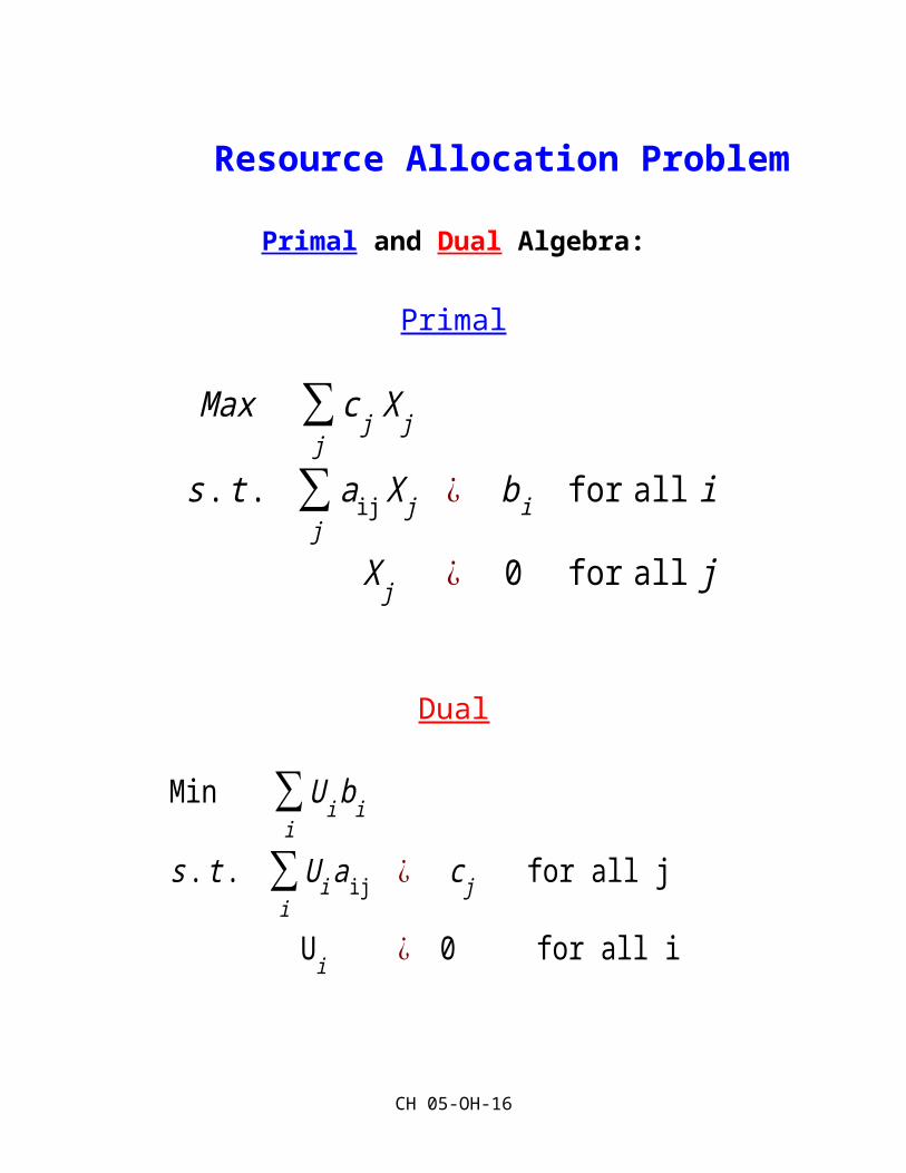
Table 5.3. First GAMS Formulation of Resource Allocation Example 1 SET PROCESS TYPES OF PRODUCTION PROCESSES

2 /FUNCTNORM , FUNCTMXSML , FUNCTMXLRG 3 ,FANCYNORM , FANCYMXSML ,FANCYMXLRG/ 4 RESOURCE TYPES OF RESOURCES 5 /SMLLATHE,LRGLATHE,CARVER,LABOR/ ; 7 PARAMETER PRICE(PROCESS) PRODUCT PRICES BY PROCESS 8 /FUNCTNORM 82, FUNCTMXSML 82, FUNCTMXLRG 82 9 ,FANCYNORM 105, FANCYMXSML 105, FANCYMXLRG 105/10 PRODCOST(PROCESS) COST BY PROCESS11 /FUNCTNORM 15, FUNCTMXSML 16, FUNCTMXLRG 15.712 ,FANCYNORM 25, FANCYMXSML 26.5,FANCYMXLRG 26.6/13 RESORAVAIL(RESOURCE) RESOURCE AVAILABLITY14 /SMLLATHE 140, LRGLATHE 90,15 CARVER 120, LABOR 125/;16 17 TABLE RESOURUSE(RESOURCE,PROCESS) RESOURCE USAGE18 19 FUNCTNORM FUNCTMXSML FUNCTMXLRG20 SMLLATHE 0.80 1.30 0.2021 LRGLATHE 0.50 0.20 1.3022 CARVER 0.40 0.40 0.4023 LABOR 1.00 1.05 1.1024 + FANCYNORM FANCYMXSML FANCYMXLRG25 SMLLATHE 1.20 1.70 0.5026 LRGLATHE 0.70 0.30 1.5027 CARVER 1.00 1.00 1.0028 LABOR 0.80 0.82 0.84;30 POSITIVE VARIABLES31 PRODUCTION(PROCESS) ITEMS PRODUCED BY PROCESS;32 VARIABLES33 PROFIT TOTALPROFIT;34 EQUATIONS35 OBJT OBJECTIVE FUNCTION ( PROFIT )36 AVAILABLE(RESOURCE) RESOURCES AVAILABLE ;37 38 OBJT.. PROFIT =E=39 SUM(PROCESS,(PRICE(PROCESS)-PRODCOST(PROCESS))40 * PRODUCTION(PROCESS)) ;42 AVAILABLE(RESOURCE)..43 SUM(PROCESS,RESOURUSE(RESOURCE,PROCESS)*PRODUCTION(PROCESS))44 =L= RESORAVAIL(RESOURCE);46 MODEL RESALLOC /ALL/;47 SOLVE RESALLOC USING LP MAXIMIZING PROFIT;

CH 05-OH-16

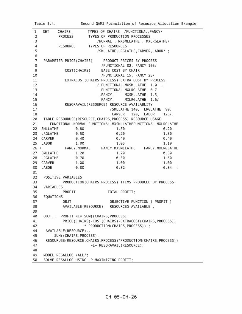
Table 5.4. Second GAMS Formulation of Resource Allocation Example

1 SET CHAIRS TYPES OF CHAIRS /FUNCTIONAL,FANCY/ 2 PROCESS TYPES OF PRODUCTION PROCESSES 3 /NORMAL , MXSMLLATHE , MXLRGLATHE/ 4 RESOURCE TYPES OF RESOURCES 5 /SMLLATHE,LRGLATHE,CARVER,LABOR/ ; 6 7 PARAMETER PRICE(CHAIRS) PRODUCT PRICES BY PROCESS 8 /FUNCTIONAL 82, FANCY 105/ 9 COST(CHAIRS) BASE COST BY CHAIR 10 /FUNCTIONAL 15, FANCY 25/ 11 EXTRACOST(CHAIRS,PROCESS) EXTRA COST BY PROCESS 12 / FUNCTIONAL.MXSMLLATHE 1.0 , 13 FUNCTIONAL.MXLRGLATHE 0.7 14 ,FANCY. MXSMLLATHE 1.5, 15 FANCY. MXLRGLATHE 1.6/ 16 RESORAVAIL(RESOURCE) RESOURCE AVAILABLITY 17 /SMLLATHE 140, LRGLATHE 90, 18 CARVER 120, LABOR 125/; 20 TABLE RESOURUSE(RESOURCE,CHAIRS,PROCESS) RESOURCE USAGE 21 FUNCTIONAL.NORMAL FUNCTIONAL.MXSMLLATHEFUNCTIONAL.MXLRGLATHE 22 SMLLATHE 0.80 1.30 0.20 23 LRGLATHE 0.50 0.20 1.30 24 CARVER 0.40 0.40 0.40 25 LABOR 1.00 1.05 1.10 26 + FANCY.NORMAL FANCY.MXSMLLATHE FANCY.MXLRGLATHE 27 SMLLATHE 1.20 1.70 0.50 28 LRGLATHE 0.70 0.30 1.50 29 CARVER 1.00 1.00 1.00 30 LABOR 0.80 0.82 0.84 ; 31 32 POSITIVE VARIABLES 33 PRODUCTION(CHAIRS,PROCESS) ITEMS PRODUCED BY PROCESS; 34 VARIABLES 35 PROFIT TOTAL PROFIT; 36 EQUATIONS 37 OBJT OBJECTIVE FUNCTION ( PROFIT ) 38 AVAILABLE(RESOURCE) RESOURCES AVAILABLE ; 39 40 OBJT.. PROFIT =E= SUM((CHAIRS,PROCESS), 41 PRICE(CHAIRS)-COST(CHAIRS)-EXTRACOST(CHAIRS,PROCESS)) 42 * PRODUCTION(CHAIRS,PROCESS)) ; 44 AVAILABLE(RESOURCE).. 45 SUM((CHAIRS,PROCESS), 46 RESOURUSE(RESOURCE,CHAIRS,PROCESS)*PRODUCTION(CHAIRS,PROCESS)) 47 =L= RESORAVAIL(RESOURCE); 48 49 MODEL RESALLOC /ALL/; 50 SOLVE RESALLOC USING LP MAXIMIZING PROFIT;

CH 05-OH-17

Transportation ProblemBasic Concept

This problem involves the shipment of a homogeneous product

from a number of supply locations to a number of demand

locations.

Supply Locations Demand Locations

1 A

2 B

… …

m n Problem: given needs at the demand locations how should I take limited supply at supply locations and move the goods to meet needs. Further suppose we wish to minimize cost.

Objective: Minimize cost

Variables Quantity of goods shipped from each supply point to each demand point

Restrictions: Non negative shipments Supply availability at supply point

Demand need at a demand point

CH 05-OH-18

Transportation ProblemFormulating the Problem

Basic notation and the decision variable

Let us denote the supply locations as supplyi

Let us denote the demand locations as demandj

Let us define our fundamental decision variable as the set

of individual shipment quantities from each supply

location to each demandlocation and denote this variable

algebraically as

Movesupplyi,demandj

CH 05-OH-19


The objective function:

We want to minimize total shipping cost so we need an

expression for shipping cost

Let us define a data item giving the per unit cost of shipments

from each supply location to each demand location as

costsupplyi,demandj

Our objective then becomes to minimize the sum of the

shipment costs over all supplyi, demandj pairs or

Minimize costsupplyi,demandjMovesupplyi,demandj

which is the per unit cost of moving from each supply location

to each demand location times the amount shipped summed over

all possible shipment routes

CH 05-OH-20


There are three types of constraints:

1) Supply availability: limiting shipments from each supplypoint to existing supply so that the sum of outgoing shipments from the supplyith supply point to all possible destinations (demandj) to not exceed supplysupplyi

2) Minimum demand: requiring shipments into the demandjth demand point be greater than or equal to demand at that point. Incoming shipments include shipments from all possible supply points supplyi to the demandjth demand point.

3) Nonnegative shipments:

CH 05-OH-21


Formulation and Example:

Explicitly :

Transportation ProblemCH 05-OH-22

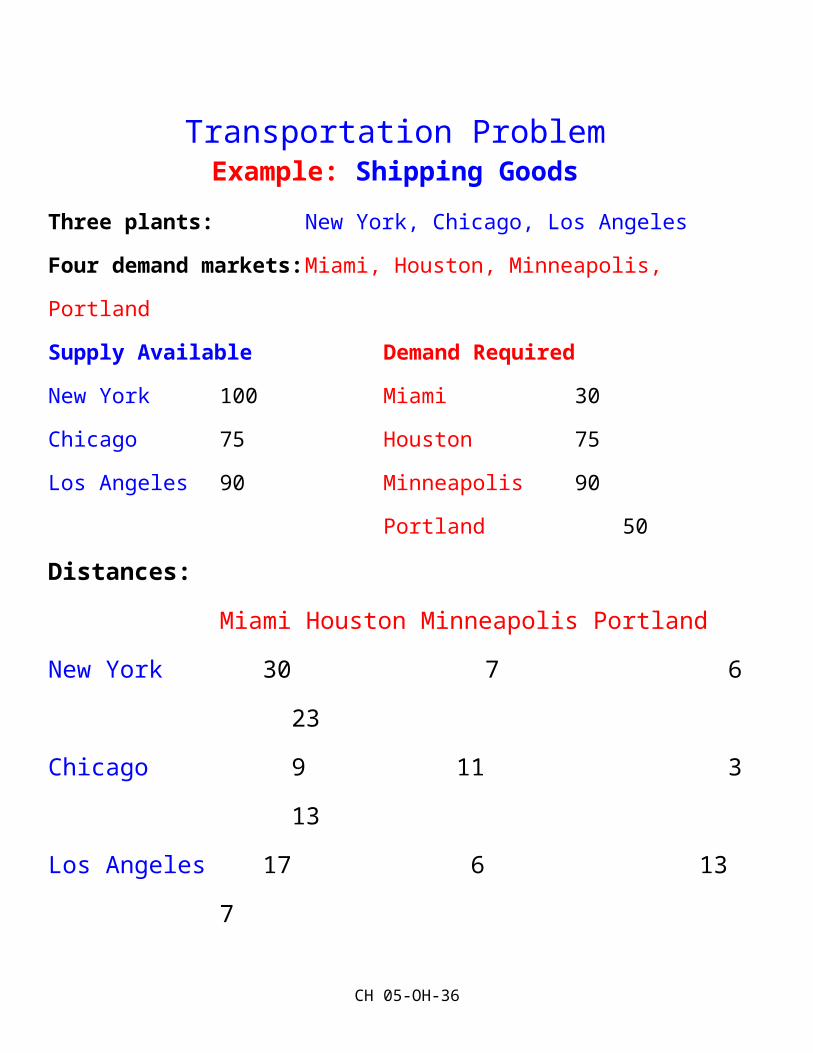
Example: Shipping GoodsThree plants: New York, Chicago, Los Angeles

Four demand markets: Miami, Houston, Minneapolis, Portland

Supply Available Demand Required

New York 100 Miami 30

Chicago 75 Houston 75

Los Angeles 90 Minneapolis 90

Portland 50

Distances:

Miami Houston Minneapolis Portland

New York 30 7 6 23

Chicago 9 11 3 13

Los Angeles 17 6 13 7

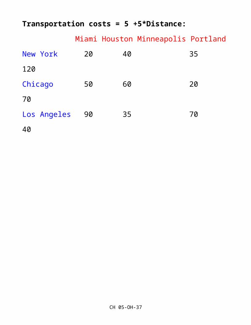
Transportation costs = 5 +5*Distance:


New York 20 40 35 120

Chicago 50 60 20 70

Los Angeles 90 35 70 40

CH 05-OH-23

Transportation ProblemExample: Shipping Goods

Min 20X11 + 40X12 + 35

X13

+ 120

X14

+ 50X21 + 60X22 + 20X23 + 70X24 + 90X31 + 35X32 + 70X33 + 40

X34s.t. X11 + X12 + X13 + X14 ≤ 100

X21 + X22 + X23 + X24 ≤ 75

X31 + X32 + X33 + X34 ≤ 90

X11 + X21 + X31 ≥ 30

X12 + X22 + X32 ≥ 75

X13 + X23 + X33 ≥ 90

X14 + X24 + X34≥ 50

Xij≥0

CH 05-OH-24

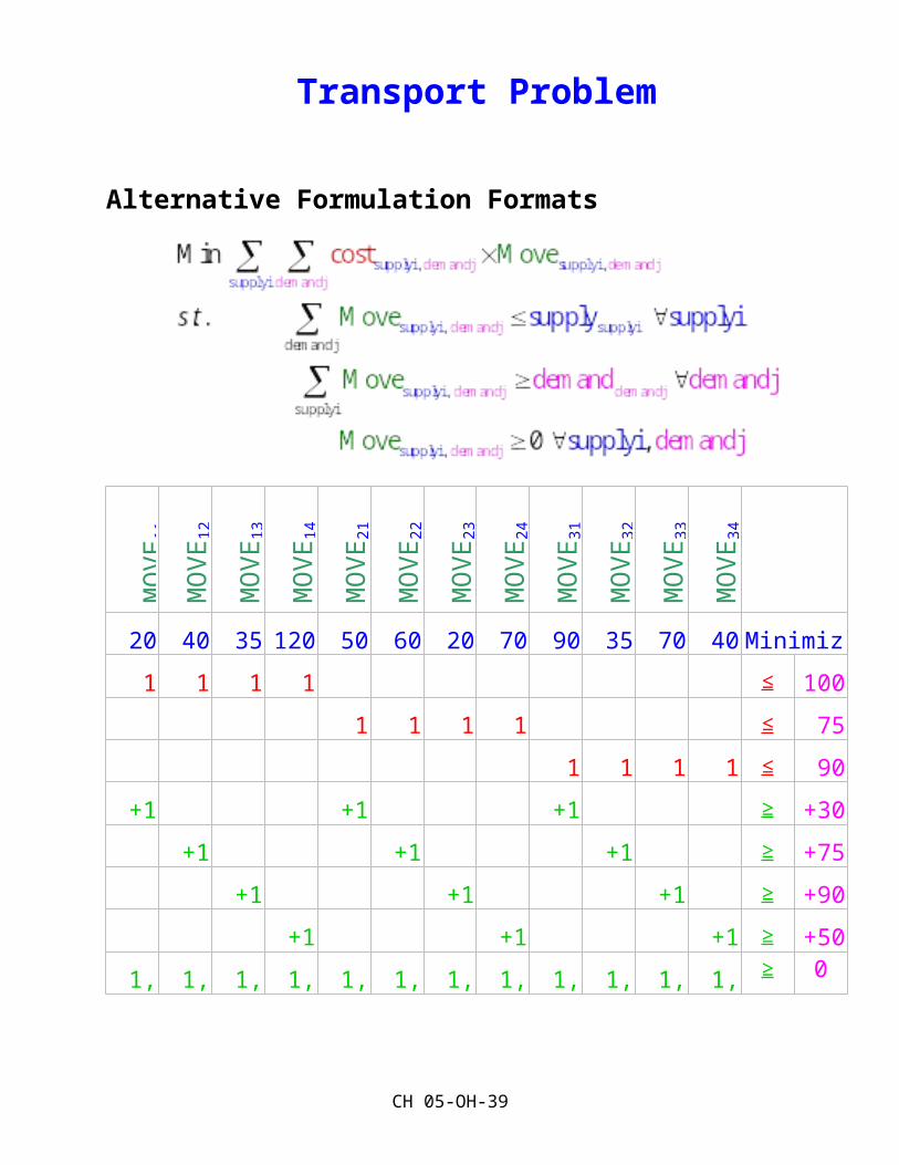
Transport Problem

Alternative Formulation FormatsM

OV

E 11

MO

VE 1

2

MO

VE 1

3

MO

VE 1

4

MO

VE 2

1

MO

VE 2

2

MO

VE 2

3

MO

VE 2

4

MO

VE 3

1

MO

VE 3

2

MO

VE 3

3

MO

VE 3

4

20 40 35 120 50 60 20 70 90 35 70 40 Minimize

1 1 1 1 ≤ 100

1 1 1 1 ≤ 75

1 1 1 1 ≤ 90

+1 +1 +1 ≥ +30

+1 +1 +1 ≥ +75

+1 +1 +1 ≥ +90

+1 +1 +1 ≥ +50

1, 1, 1, 1, 1, 1, 1, 1, 1, 1, 1, 1, ≥ 0

CH 05-OH-25

Transportation ProblemExample: Shipping Goods – Solution

- shadow price represents marginal values of theresources i.e. marginal value of additional units in Chicago = $15

- reduced cost represents marginal costs of forcingnon-basic variable into the solution i.e. shipments from New York to Portland costs $75

- twenty units are left in New York

Optimal Solution: Objective value $7,425

Table 5.8. Optimal Solution to the ABC Company Problem

Variable Value Reduced Cost Equation Slack Shadow Price

Move11 30 0 1 20 0Move12 35 0 2 0 -15Move13 15 0 3 0 -5Move14 0 75 4 0 20Move21 0 45 5 0 40Move22 0 35 6 0 35Move23 75 0 7 0 45Move24 0 40Move31 0 75Move32 40 0Move33 0 40Move34 50 0

Optimal Shipping Patterns

Origin

Destination


Units Variable Units Variable Units Variable Units Variable

New York 30 Move11 35 Move12 15 Move13

Chicago 75 Move23

Los Angeles 40 Move32 50 Move34

CH 05-OH-26

Transport ProblemPrimal and Dual Algebra:

Primal

Dual

CH 05-OH-27

Transport ProblemEmpirical Primal and Dual

Primal

20 40 35 120 50 60 20 70 90 35 70 40 Minimize1 1 1 1 ≤ 100

1 1 1 1 ≤ 751 1 1 1 ≤ 90

+1 +1 +1 ≥ +30+1 +1 +1 ≥ +75

+1 +1 +1 ≥ +90+1 +1 +1 ≥ +50

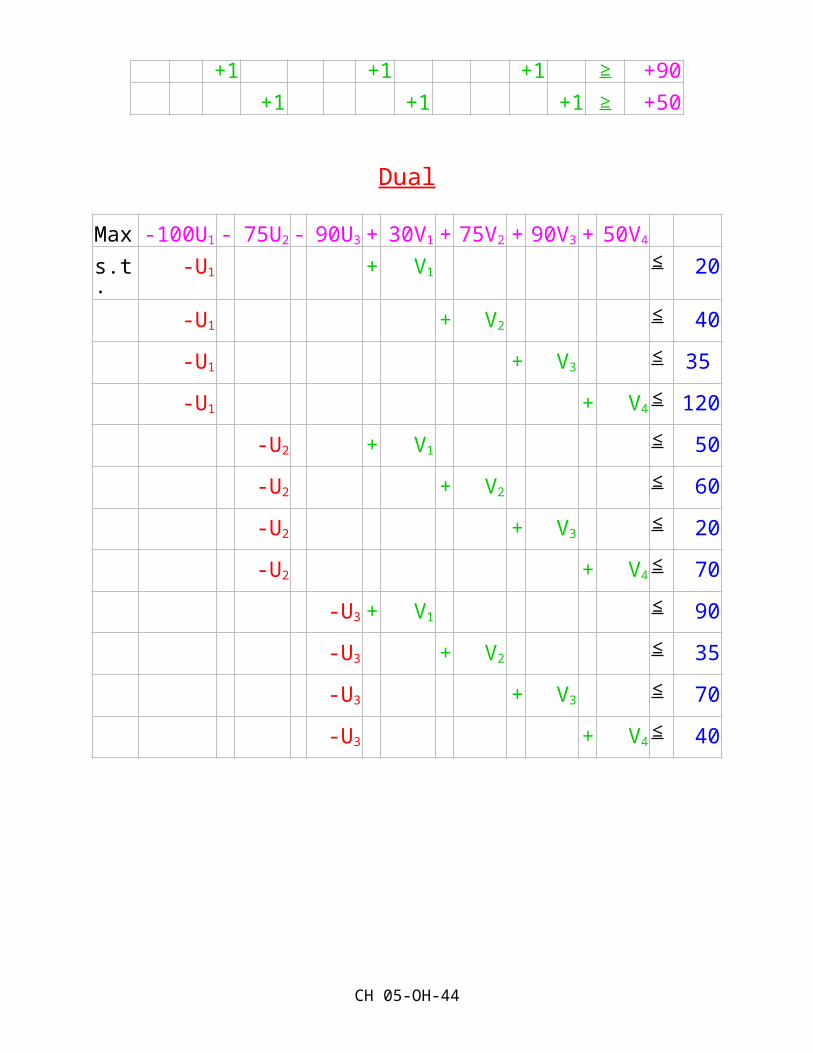
Dual

Max -100U1 - 75U2 - 90U3 + 30V1 + 75V2 + 90V3 + 50V4

s.t. -U1 + V1≤ 20

-U1 + V2≤ 40

-U1 + V3≤ 35

-U1 + V4≤ 120

-U2 + V1≤ 50

-U2 + V2≤ 60

-U2 + V3≤ 20

-U2 + V4≤ 70

-U3 + V1≤ 90

-U3 + V2≤ 35

CH 05-OH-28

-U3 + V3≤ 70

-U3 + V4≤ 40

CH 05-OH-29

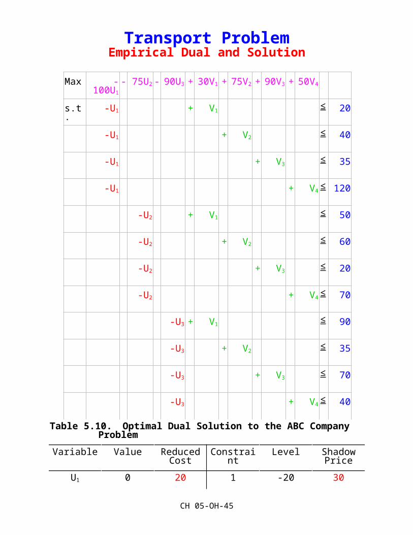
Transport ProblemEmpirical Dual and Solution

Max -100U1 - 75U2 - 90U3 + 30V1 + 75V2 + 90V3 + 50V4

s.t. -U1 + V1 ≤ 20

-U1 + V2 ≤ 40

-U1 + V3 ≤ 35

-U1 + V4 ≤ 120

-U2 + V1 ≤ 50

-U2 + V2 ≤ 60

-U2 + V3 ≤ 20

-U2 + V4 ≤ 70

-U3 + V1 ≤ 90

-U3 + V2 ≤ 35

-U3 + V3 ≤ 70

-U3 + V4 ≤ 40

Table 5.10. Optimal Dual Solution to the ABC Company ProblemVariable Value Reduced

CostConstraint Level Shadow

Price

U1 0 20 1 -20 30U2 15 0 2 40 35U3 5 0 3 35 15V1 20 0 4 45 0V2 40 0 5 5 0

CH 05-OH-30

V3 35 0 6 25 0V4 45 0 7 20 75

8 30 09 15 010 35 4011 30 012 40 50

CH 05-OH-31

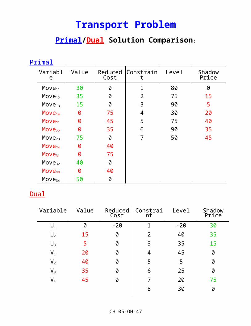
Transport ProblemPrimal/Dual Solution Comparison:

PrimalVariable Value Reduced

CostConstraint Level Shadow Price

Move11 30 0 1 80 0Move12 35 0 2 75 15Move13 15 0 3 90 5Move14 0 75 4 30 20Move21 0 45 5 75 40Move22 0 35 6 90 35Move23 75 0 7 50 45Move24 0 40Move31 0 75Move32 40 0Move33 0 40Move34 50 0

Dual

Variable Value Reduced Cost

Constraint Level Shadow Price

U1 0 -20 1 -20 30U2 15 0 2 40 35U3 5 0 3 35 15V1 20 0 4 45 0V2 40 0 5 5 0V3 35 0 6 25 0V4 45 0 7 20 75

8 30 09 15 010 35 4011 30 0

CH 05-OH-32

12 40 50

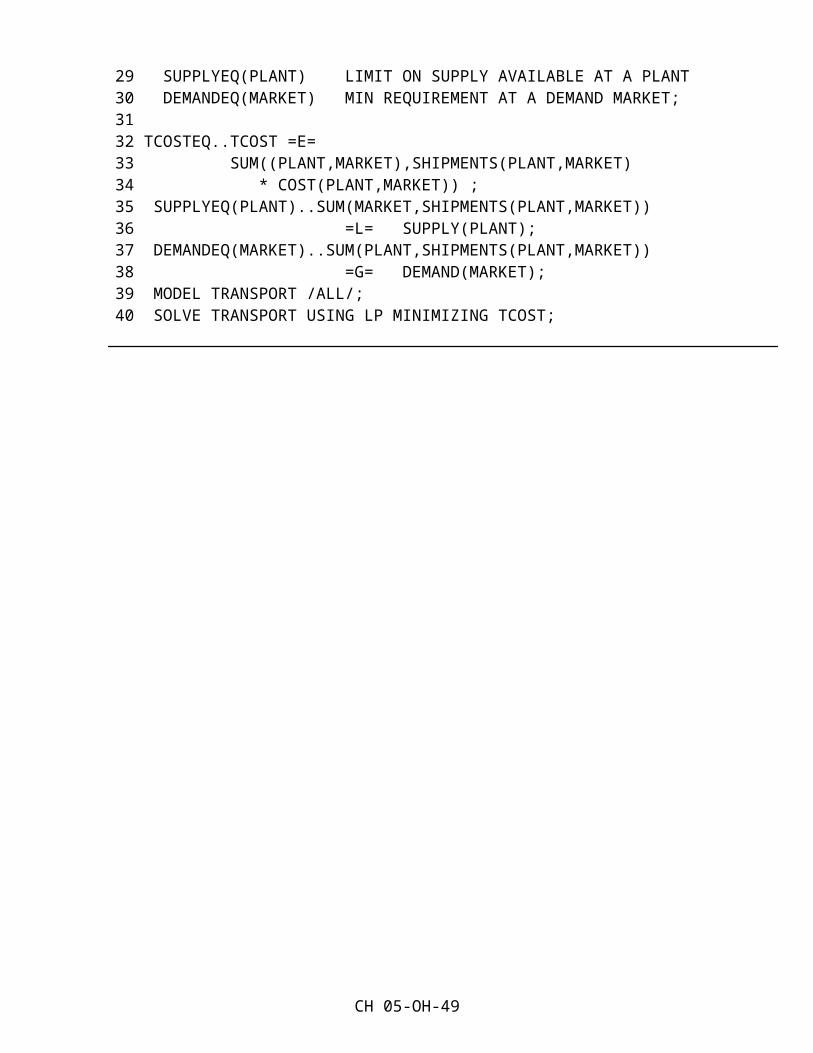
Transport ProblemTable 5.7. GAMS Statement of Transportation Example

1 SETS PLANT PLANT LOCATIONS 2 /NEWYORK, CHICAGO, LOSANGLS/ 3 MARKET DEMAND MARKETS 4 /MIAMI, HOUSTON, MINEPLIS, PORTLAND/ 5 6 PARAMETERS SUPPLY(PLANT) QUANT AVAILABLE AT EACH PLANT 7 /NEWYORK 100, CHICAGO 75, LOSANGLS 90/ 8 DEMAND(MARKET) QUANT REQUIRED BY DEMAND MARKET 9 /MIAMI 30, HOUSTON 75, 10 MINEPLIS 90, PORTLAND 50/; 11 12 TABLE DISTANCE(PLANT,MARKET) DIST FROM PLANT TO MARKET 13 14 MIAMI HOUSTON MINEPLIS PORTLAND 15 NEWYORK 3 7 6 23 16 CHICAGO 9 11 3 13 17 LOSANGLS 17 6 13 7; 18 19 20 PARAMETER COST(PLANT,MARKET) CALC COST OF MOVING GOODS ; 21 COST(PLANT,MARKET) = 5 + 5 * DISTANCE(PLANT,MARKET) ; 22 23 POSITIVE VARIABLES 24 SHIPMENTS(PLANT,MARKET) AMOUNT SHIPPED OVER A ROUTE; 25 VARIABLES 26 TCOST TOTAL COST OF SHIPPING OVER ALL ROUTES; 27 EQUATIONS 28 TCOSTEQ TOTAL COST ACCOUNTING EQUATION 29 SUPPLYEQ(PLANT) LIMIT ON SUPPLY AVAILABLE AT A PLANT 30 DEMANDEQ(MARKET) MIN REQUIREMENT AT A DEMAND MARKET; 31 32 TCOSTEQ..TCOST =E= 33 SUM((PLANT,MARKET),SHIPMENTS(PLANT,MARKET) 34 * COST(PLANT,MARKET)) ; 35 SUPPLYEQ(PLANT)..SUM(MARKET,SHIPMENTS(PLANT,MARKET)) 36 =L= SUPPLY(PLANT); 37 DEMANDEQ(MARKET)..SUM(PLANT,SHIPMENTS(PLANT,MARKET)) 38 =G= DEMAND(MARKET); 39 MODEL TRANSPORT /ALL/; 40 SOLVE TRANSPORT USING LP MINIMIZING TCOST;

CH 05-OH-33

CH 05-OH-34

Feed Mix Problem

Basic Concept

This problem involves composing a minimum cost diet from a set of

available ingredients while maintaining nutritional characteristics within

certain bounds.

Objective:Minimize total diet costs

Variables: how much of each feedstuff is used in the diet

Restrictions: Non negative feedstuff

Minimum requirements by nutrient

Maximum requirements by nutrient

Total volume of the diet

This problem requires two types of indices:

Type of feed ingredients available from which the diet can be

composed

CH 05-OH-35

ingredientj = {corn, soybeans, salt, etc.}

Type of nutritional characteristics which must fall within certain limits

nutrient = {protein, calories, etc.}

CH 05-OH-36

Feed Mix ProblemBasic Concept

Variable -- Feed ingredientj amount of feedstuff

ingredientj fed to animal

Objective – total cost

We want to minimize total diet costs across all the feedstuffs so we need

an expression for feedstuff costs.

Let us define a data item giving the per unit cost of ingredients as

costingredientj.

Our objective then becomes to minimize the sum of the diet costs over

all feed ingredients

Minimize costingredientj Feedingredientj

which is the per unit cost of ingredients summed over the feed

CH 05-OH-37

ingredients.

CH 05-OH-38

Feed Mix ProblemBasic Concept

Additional parameters representing how much of each nutrient is present in each

feedstuff as well as the dietary minimum and maximum requirements for that

nutrient are needed.

Let

1). anutrient,ingredientj be the amount of the

nutrientth nutrient present in one unit of the

ingredientjth feed ingredient

2). ULnutrient and LLnutrient be the maximum and

minimum amount of the nutrientth nutrient

in the diet

Then the nutrient constraints are formed by summing the nutrients generated from

each feedstuff (anutrient,ingredientjFingredientj) and requiring these to exceed

the dietary minimum and/or be less than the maximum.

Problem then focuses on how much of each feedstuff is used in the diet to

maintain nutritional characteristics within certain bounds.

CH 05-OH-39

Feed Mix ProblemFormulating the Problem

There are four general types of constraints:

1) minimum nutrient requirements restricting the sum of the nutrients generated from each feedstuff (anutrient,ingredientjFingredientj) to meet the dietary minimum

2) maximum nutrient requirements restricting the sum of the nutrients generated from each feedstuff (anutrient,ingredientjFingredientj) to not exceed the dietarymaximum

3) total volume of the diet constraint requiring the ingredients in the diet equal the required weight ofthe diet. Suppose the weight of the formulated diet and the feedstuffs are the same, then

4) nonnegative feedstuff

CH 05-OH-40

Feed Mix ProblemExample: cattle feeding

Seven nutritional characteristics:energy, digestible protein, fat, vitamin A, calcium, salt, phosphorus

Seven feed ingredient availability:

corn, hay, soybeans, urea, dical phosphate, salt, vitamin A

New product: potato slurry

Ingredient costs per kilogram (cingredientj)

Ingredient Costs for Diet Problem Example per kg

Corn $0.133Dical $0.498Alfalfa hay $0.077Salt $0.110Soybeans $0.300Vitamin A $0.286Urea $0.332Required Nutrient Characteristics per KilogramNutrient Unit Minimum

Amount

Maximum

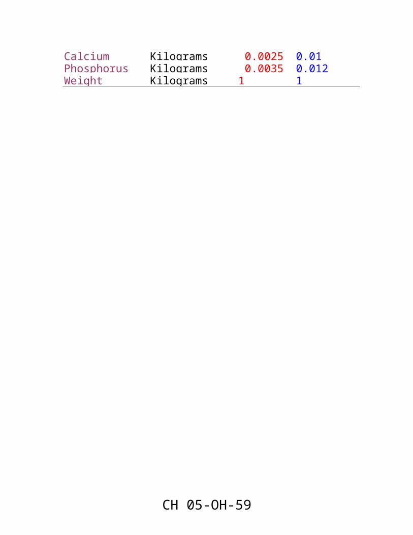
AmountNet energy Mega calories 1.34351 --Digestible protein Kilograms 0.071 0.13Fat Kilograms -- 0.05Vitamin A International Units 2200 --Salt Kilograms 0.015 0.02Calcium Kilograms 0.0025 0.01Phosphorus Kilograms 0.0035 0.012Weight Kilograms 1 1

CH 05-OH-41


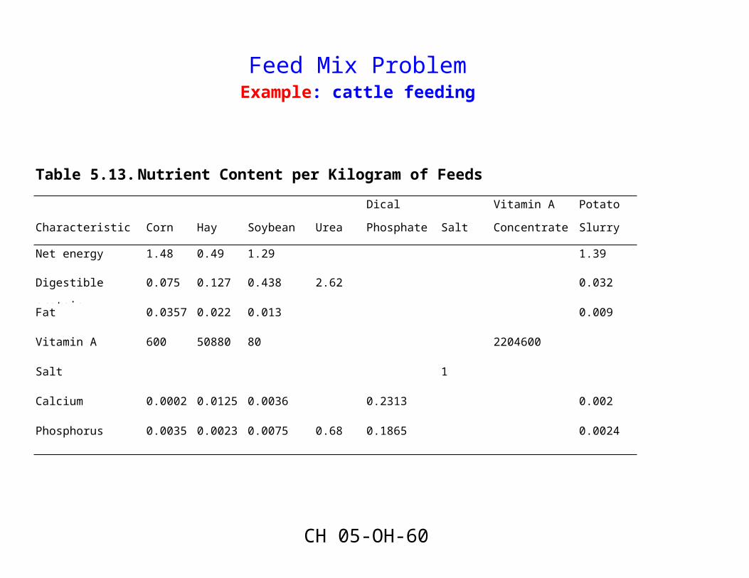
Table 5.13. Nutrient Content per Kilogram of Feeds

Characteristic Corn Hay Soybean Urea

Dical

Phosphate Salt

Vitamin A

Concentrate

Potato

Slurry

Net energy 1.48 0.49 1.29 1.39

Digestible protein 0.075 0.127 0.438 2.62 0.032

Fat 0.0357 0.022 0.013 0.009

Vitamin A 600 50880 80 2204600

Salt 1

Calcium 0.0002 0.0125 0.0036 0.2313 0.002

Phosphorus 0.0035 0.0023 0.0075 0.68 0.1865 0.0024

CH 05-OH-42


Table 5.14. Primal Formulation of Feed Problem

Corn Hay Soybean Urea Dical Salt Vitamin A Slurry

Min .133XC + .077XH + .3XSB + .332XUr + .498Xd + .110XSLT + .286XVA + PXSL

Protein .075XC + .127XH + .438XSB + 2.62XUr + .032XSL ≤ .13

Fat .0357XC + .022XH + .013XSB + .009XSL ≤ .05

Salt XSLT ≤ .02

Calcium .0002XC + .0125XH + .0036XSB + .2313Xd + .002XSL ≤ .01

Phosphorus .0035XC + .0023XH + .0075XSB + .68XUr + .1865Xd + .0024XSL ≤ .012

Energy 1.48XC + .49XH + 1.29XSB + 1.39XSL ≥ 1.34351

Protein .075XC + .127XH + .438XSB + 2.62XUr + .032XSL ≥ .071

Vit A 600XC + 50880XH + 80XSB + 2204600XVA ≥ 2200

Salt XSLT ≥ .015

Calcium .0002XC + .0125XH + .0036XSB + .2313Xd + .002XSL ≥ .0025

Phosphorus .0035XC + .0023XH + .0075XSB + .68XUr + .1865Xd + .0024XSL ≥ .0035

Volume XC + XH + XSB + XUr + Xd + XSLT + XVA + XSL = 1

CH 05-OH-43

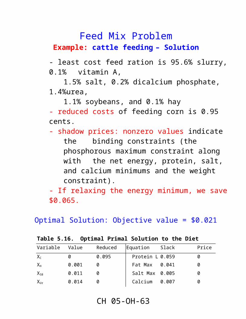
Feed Mix ProblemExample: cattle feeding – Solution

- least cost feed ration is 95.6% slurry, 0.1% vitamin A, 1.5% salt, 0.2% dicalcium phosphate, 1.4%urea, 1.1% soybeans, and 0.1% hay

- reduced costs of feeding corn is 0.95 cents.- shadow prices: nonzero values indicate the binding

constraints (the phosphorous maximum constraint along with the net energy, protein, salt, and calcium minimums and the weight constraint).

- If relaxing the energy minimum, we save $0.065.

Optimal Solution: Objective value = $0.021

Table 5.16. Optimal Primal Solution to the Diet Example ProblemVariable Value Reduced Cost Equation Slack Price

XC 0 0.095 Protein L Max 0.059 0

XH 0.001 0 Fat Max 0.041 0

XSB 0.011 0 Salt Max 0.005 0

XUr 0.014 0 Calcium Max 0.007 0

Xd 0.002 0 Phosphrs 0.000 -2.207

XSLT 0.015 0 Net Engy Min 0.000 0.065

XVA 0.001 0 Protein Min 0.000 0.741

XSL 0.956 0 Vita Lim Min 0.000 0

Salt Lim Min 0.000 0.218

Calcium Min .000 4.400

Phosphrs 0.008 0

Weight 0.000 -0.108

CH 05-OH-44

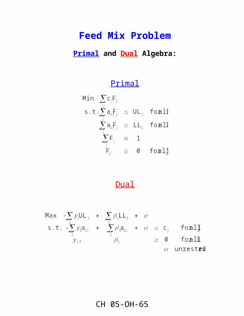
Feed Mix ProblemPrimal and Dual Algebra:

Primal

Dual

CH 05-OH-45

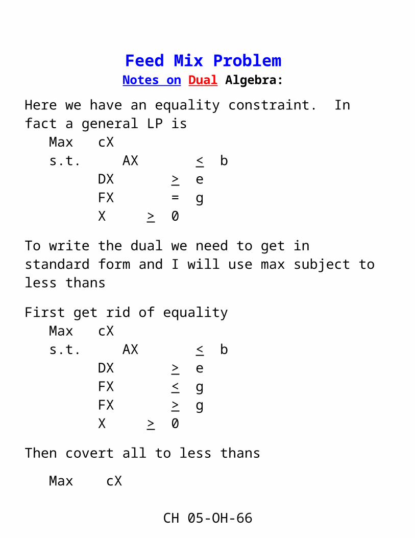
Feed Mix ProblemNotes on Dual Algebra:

Here we have an equality constraint. In fact a general LP is Max cXs.t. AX < b

DX > eFX = gX > 0

To write the dual we need to get in standard form and I will use max subject to less thans

First get rid of equalityMax cXs.t. AX < b

DX > eFX < gFX > gX > 0

Then covert all to less thans

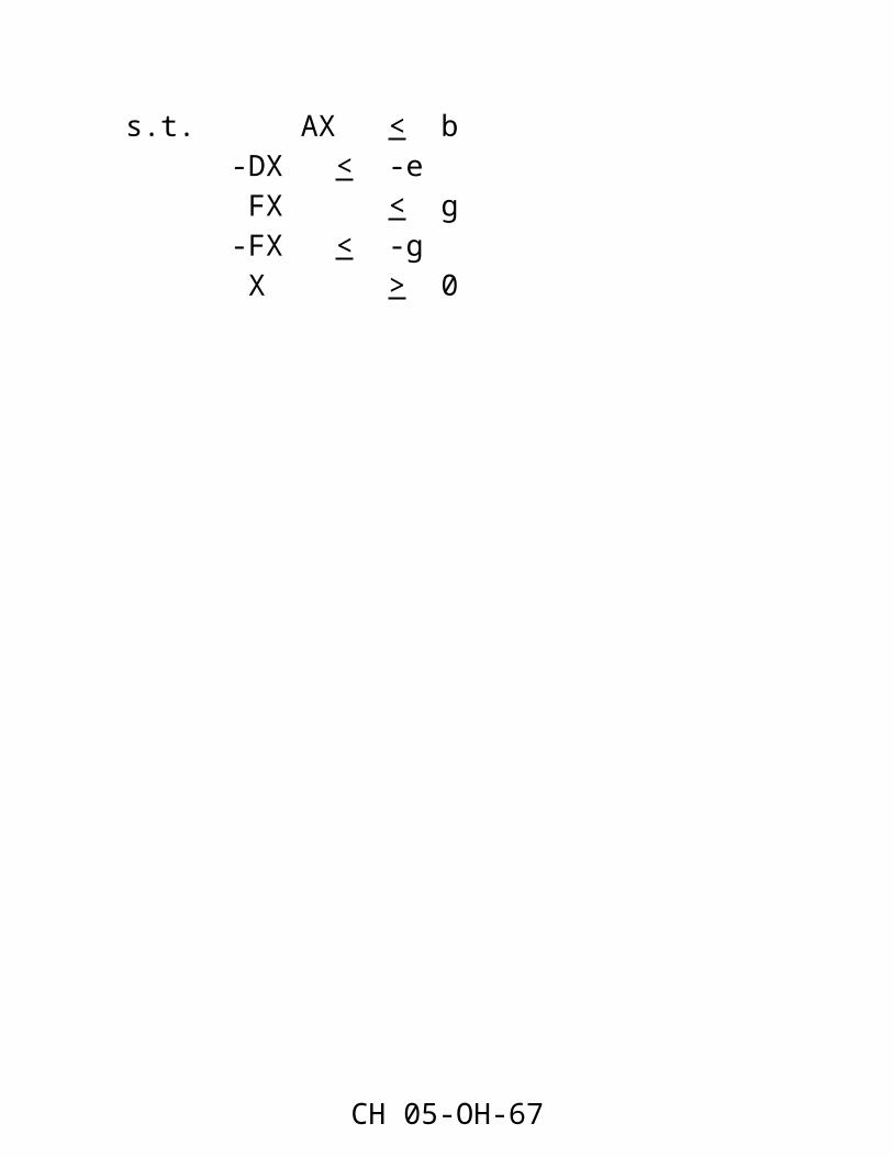
Max cXs.t. AX < b

-DX < -e FX < g-FX < -g X > 0

CH 05-OH-46

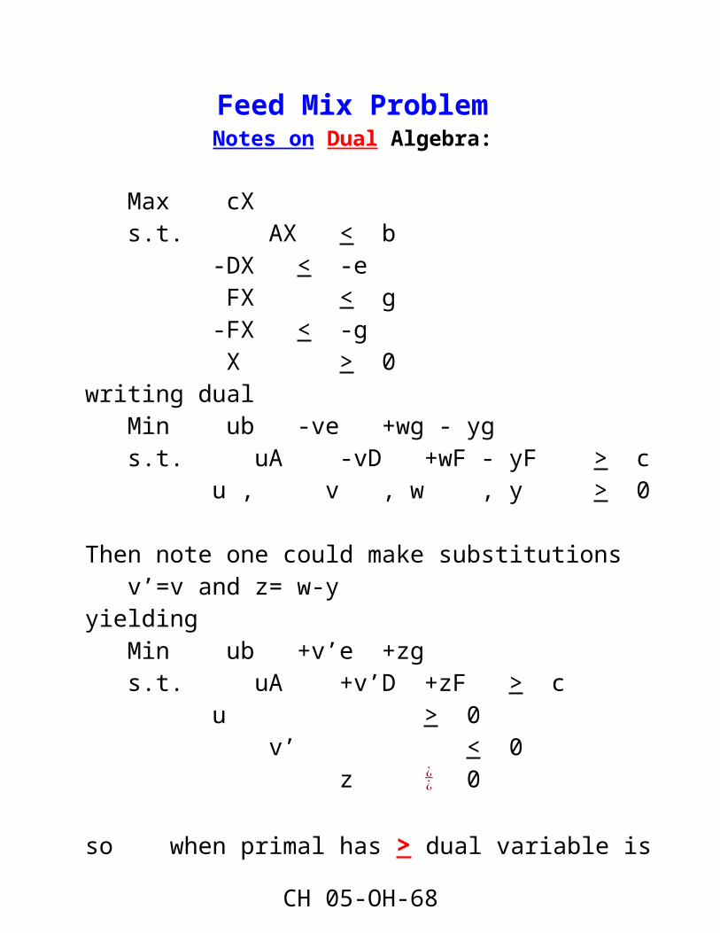
Feed Mix ProblemNotes on Dual Algebra:

Max cXs.t. AX < b

-DX < -e FX < g-FX < -g X > 0

writing dual Min ub -ve +wg - ygs.t. uA -vD +wF - yF > c

u , v , w , y > 0

Then note one could make substitutions v’=v and z= w-y

yieldingMin ub +v’e +zgs.t. uA +v’D +zF > c

u > 0 v’ < 0

z ¿¿ 0

so when primal has > dual variable is negative and when primal has = dual variable is unrestricted in sign

CH 05-OH-47

Feed Mix ProblemDual and Example

Table 5.17. Dual Formulation of Feed Mix Example Problem

γ1 γ 2 γ 3 γ 4 γ 5 β 1 β 2 β 3 β 4 β 5 β 6 α

Max - .13 - .05 - .02 - .01 - .12 + 1.34351 + .071 + 2200 + .015 + .0025 + .0035 + 1

- .075 - .0357 - .0002 - .0035 + 1.48 + .075 + 600 + .0002 + .0035 + 1 ≤ .133

- .127 - .022 - .0125 - .0023 + .49 + .127 + 50880 + .0125 + .0023 + 1 ≤ .077

- .438 - .013 - .0036 - .0075 + 1.29 + .438 + 80 + .0036 + .0075 + 1 ≤ .3

-2.62 - .68 + 2.62 + .68 + 1 ≤ .332

- .2313 - .1865 + .2313 + .1865 + 1 ≤ .498

- 1 + 1 + 1 ≤ .110

+ 2204600 + 1 ≤ .286

- .032 - .009 - .002 - .0024 + 1.39 + .032 + .002 + .0024 + 1 ≤ P

Feed Mix ProblemCH 05-OH-48

Primal / Dual Empirical Comparison:Table 5.14. Primal Formulation of Feed Problem

Corn Hay Soybean Urea Dical Salt Vitamin A Slurry

Min .133XC + .077XH + .3XSB + .332XUr + .498Xd + .110XSLT + .286XVA + PXSL

s.t. .075XC + .127XH + .438XSB + 2.62XUr + .032XSL ≤ .13

Max .0357XC + .022XH + .013XSB + .009XSL ≤ .05

Nut XSLT ≤ .02

.0002XC + .0125XH + .0036XSB + .2313Xd + .002XSL ≤ .01

.0035XC + .0023XH + .0075XSB + .68XUr + .1865Xd + .0024XSL ≤ .012

1.48XC + .49XH + 1.29XSB + 1.39XSL ≥ 1.34351

.075XC + .127XH + .438XSB + 2.62XUr + .032XSL ≥ .071

Min 600XC + 50880XH + 80XSB + 2204600XVA ≥ 2200

Nut XSLT ≥ .015

.0002XC + .0125XH + .0036XSB + .2313Xd + .002XSL ≥ .0025

.0035XC + .0023XH + .0075XSB + .68XUr + .1865Xd + .0024XSL ≥ .0035

Volume XC + XH + XSB + XUr + Xd + XSLT + XVA + XSL = 1

CH 05-OH-49

Feed Mix ProblemPrimal / Dual Empirical Comparison:

≤Dual:

Table 5.17. Dual Formulation of Feed Mix Example Problem

γ1 γ 2 γ 3 γ 4 γ 5 β 1 β 2 β 3 β 4 β 5 β 6 α

Max - .13 - .05 - .02 - .01 - .12 + 1.34351 + .071 + 2200 + .015 + .0025 + .0035 + 1

- .075 - .0357 - .0002 - .0035 + 1.48 + .075 + 600 + .0002 + .0035 + 1 ≤ .133

- .127 - .022 - .0125 - .0023 + .49 + .127 + 50880 + .0125 + .0023 + 1 ≤ .077

- .438 - .013 - .0036 - .0075 + 1.29 + .438 + 80 + .0036 + .0075 + 1 ≤ .3

-2.62 - .68 + 2.62 + .68 + 1 ≤ .332

- .2313 - .1865 + .2313 + .1865 + 1 ≤ .498

- 1 + 1 + 1 ≤ .110

+ 2204600 + 1 ≤ .286

- .032 - .009 - .002 - .0024 + 1.39 + .032 + .002 + .0024 + 1 ≤ P

CH 05-OH-50

Feed Mix ProblemPrimal / Dual Solution Comparison

Table 5.16. Optimal Primal Solution to the Diet Example Problem

Variable Value Reduced Cost

Constraint Level Price

XC 0 0.095 Protein L Max 0.071 0

XH 0.001 0 Fat Max 0.009 0

XSB 0.011 0 Salt Max 0.015 0

XUr 0.014 0 Calcium Max 0.002 0

Xd 0.002 0 Phosphrs 0.012 -2.207

XSLT 0.015 0 Net Engy Min 1.344 0.065

XVA 0.001 0 Protein Min 0.071 0.741

XSL 0.956 0 Vita Lim Min 2200.0 0

Salt Lim Min 0.015 0.218Calcium Min .002 4.400Phosphrs 0.012 0Weight 1 -0.108

Table 5.18. Optimal Solution to the Dual of the Feed Mix Problem

Variable Value Reduced Cost Constraint Level Shadow Price

γ1 0 -0.059 Corn 0.038 0

γ2 0 -0.041 Hay 0.077 0.001

γ3 0 -0.005 Soybean 0.300 0.011

γ4 0 -0.007 Orea 0.332 0.014

γ5 2.207 0 Dical 0.498 0.002

CH 05-OH-51

β1 0.065 0 Salt 0.110 0.015

β2 0.741 0 Vita 0.286 0.001

β3 0 0 Slurry 0.01 0.956

β4 0.218 0

β5 4.400 0

β6 0 -0.008

Α -0.108 0

Feed Mix ProblemCost Ranging Result

CH 05-OH-52

Feed Mix ProblemTable 5.15 GAMS Formulation of Diet Example

1 SET INGREDT NAMES OF THE AVAILABLE FEED INGREDIENTS 2 /CORN,HAY,SOYBEAN,UREA,DICAL,SALT,VITA,SLURRY/ 3 NUTRIENT NUTRIENT REQUIREMENT CATEGORIES 4 /NETENGY,PROTEIN,FAT,VITALIM,SALTLIM,CALCIUM, PHOSPHRS/ 5 LIMITS TYPES OF LIMITS IMPOSED ON NUTRIENTS /MIN,MAX/; 6 PARAMETER INGREDCOST(INGREDT) INGREDIENT COSTS PER KG BOUGHT 7 /CORN .133, HAY .077, SOYBEAN .300, UREA .332 8 , DICAL .498,SALT .110, VITA .286, SLURRY .01/; 9 TABLE NUTREQUIRE(NUTRIENT, LIMITS) NUTRIENT REQUIREMENTS 10 MIN MAX 11 NETENGY 1.34351 12 PROTEIN .071 .130 13 FAT 0 .05 14 VITALIM 2200 15 SALTLIM .015 .02 16 CALCIUM .0025 .0100 17 PHOSPHRS .0035 .0120; 18 TABLE CONTENT(NUTRIENT,INGREDT) NUTR CONTENTS PER KG OF FEED 19 CORN HAY SOYBEAN UREA DICAL SALT VITA SLURRY 20 NETENGY 1.48 .49 1.29 1.39 21 PROTEIN .075 .127 .438 2.62 0.032 22 FAT .0357 .022 .013 0.009 23 VITALIM 600 50880 80 2204600 24 SALTLIM 1 25 CALCIUM .0002 .0125 .0036 .2313 .002 26 PHOSPHRS 0035 .0023 .0075 .68 .1865 .0024; 27 28 POSITIVE VARIABLES 29 FEEDUSE(INGREDT) AMOUNT OF EACH INGREDIENT USED IN MIXING FEED; 30 VARIABLES 31 COST PER KG COST OF THE MIXED FEED; 32 EQUATIONS 33 OBJT OBJECTIVE FUNCTION ( TOTAL COST OF THE FEED ) 34 MAXBD(NUTRIENT) MAX LIMITS ON EACH NUTRIENT IN THE BLENDED FEED 35 MINBD(NUTRIENT) MIN LIMITS ON EACH NUTRIENT IN THE BLENDED FEED 36 WEIGHT REQUIRED THAT EXACTLY ONE KG OF FEED BE PRODUCED; 37 38 OBJT..COST =E= SUM(INGREDT,INGREDCOST(INGREDT)* FEEDUSE(INGREDT)) 39 MAXBD(NUTRIENT)$NUTREQUIRE(NUTRIENT,"MAXIMUM").. 40 SUM(INGREDT,CONTENT(NUTRIENT , INGREDT) * FEEDUSE(INGREDT)) 41 =L= NUTREQUIRE(NUTRIENT, "MAXIMUM"); 42 MINBD(NUTRIENT)$NUTREQUIRE(NUTRIENT,"MINIMUM").. 43 SUM(INGREDT,CONTENT(NUTRIENT, INGREDT) * FEEDUSE(INGREDT)) 44 =G= NUTREQUIRE(NUTRIENT, "MINIMUM"); 45 WEIGHT.. SUM(INGREDT, FEEDUSE(INGREDT)) =E= 1. ;

46 MODEL FEEDING /ALL/; 47 SOLVE FEEDING USING LP MINIMIZING COST; 48 49 SET VARYPRICE PRICE SCENARIOS /1*30/ 50 PARAMETER SLURR(VARYPRICE,*) 51 OPTION SOLPRINT = OFF; 52 LOOP (VARYPRICE, 53 INGREDCOST("SLURRY")= 0.01 + (ORD(VARYPRICE)-1)*0.005; 54 SOLVE FEEDING USING LP MINIMIZING COST; 55 SLURR(VARYPRICE,"SLURRY") = FEEDUSE.L("SLURRY"); 56 SLURR(VARYPRICE,"PRICE") = INGREDCOST("SLURRY") ) ; 57 DISPLAY SLURR;

CH 05-OH-54

Joint Products Problem

Formulation

Basic notation and the decision variable

Let us denote the set of

: the produced products as product

: the production possibilities as process

: the purchased inputs as input

: the available resources as resource

Let us define three fundamental decision variables as

: the set of produced product,

Salesproduct

CH 05-OH-31

: the set of production possibilities,

Productionprocess

: the set of purchased inputs,

BuyInputinput

CH 05-OH-32

Joint Products ProblemFormulation

To set up the joint products problem, four additional parameter

values that give the composite relationship among product,

process, input, and resource are needed.

These parameters are:

the quantity yielded by the production possibility, qproduct,process

the amount of the inputth input used by the processth production

possibility, rinput,process

the amount of the resourceth resource used by the processth

production possibility, sresource,process

the amount of resource availability or endowment by resource,

bresource

CH 05-OH-33

Joint Products ProblemFormulating the Problem

The objective function:

We want to maximize total profits across all of the possible productions. To do so, three additional required parameters for sale price, input purchase cost, and other production costs associated with production are needed.

Let us define these parameters as

SalePriceproduct

InputCostinput

OtherCostprocess

Then the objective function becomes

Maximize

CH 05-OH-34

CH 05-OH-35


The constraints:

There are four general types of constraints:

1) demand and supply balance for which quantity sold of each product is

less than or equal to the quantity yielded by production.

2) demand and supply balance for which quantity purchased of each

fixed price input is greater than or equal to the quantity utilized by the

production activities.

3) resource availability constraint insuring that the quantity used of each

fixed quantity input does not exceed the resource endowments.

4)

4) nonnegativity

CH 05-OH-36


Maximize

s.t.

CH 05-OH-37

Joint Products ProblemExample: wheat production

Two products produced: Wheat and wheat straw

Three inputs: Land, fertilizer, seed

Seven production processes:

Outputs and Inputs Per Acre Process

1 2 3 4 5 6 7

Wheat yield in bu. 30 50 65 75 80 80 75

Wheat straw yield/bales 10 17 22 26 29 31 32

Fertilizer use in Kg. 0 5 10 15 20 25 30

Seed in pounds 10 10 10 10 10 10 10

Land 1 1 1 1 1 1 1

Wheat price = $4/bushel, wheat straw price =$0.5/bale

Fertilizer = $2 per kg, Seed = $0.2/lb.

$5 per acre production cost for each process

Land = 500 acres

CH 05-OH-39

Joint Products ProblemExample: Wheat Production

Maximize

s.t.

CH 05-OH-40

CH 05-OH-41

Joint Products ProblemExample: Wheat Production

4Sale1 + .5Sale2 - 5Y1 - 5Y2 - 5Y3 - 5Y4 - 5Y5 - 5Y6 - 5Y7 - 2Z1 - .2Z2 MAX

s.t. Sale1 - 30Y1 - 50Y2 - 65Y3 - 75Y4 - 80Y5 - 80Y6 - 75Y7 ≤ 0

Sale2 - 10Y1 - 17Y2 - 22Y3 - 26Y4 - 29Y5 - 31Y6 - 32Y7 ≤ 0

+ 5Y2 + 10Y3 + 15Y4 + 20Y5 + 25Y6 + 30Y7 - Z1 ≤ 0

10Y1 + 10Y2 + 10Y3 + 10Y4 + 10Y5 + 10Y6 + 10Y7 - Z2 ≤ 0

Y1 + Y2 + Y3 + Y4 + Y5 + Y6 + Y7 ≤ 500

Sale1 , Sale2 , Y1 , Y2 , Y3 , Y4 , Y5 , Y6 , Y7 , Z1 , Z2 ≥ 0

Note that: Y refers to Productionprocess and Z refers to BuyInputinput

CH 05-OH-43

Joint Products ProblemExample: Wheat Production – Solution

- 40,000 bushels of wheat and 14,500 bales of straw are

produced by 500 acres of the fifth production possibility using

10,000 kilograms of fertilizer and 5,000 lbs. of seed

- reduced cost shows a $169.50 cost if the first production

possibility is used.

- shadow prices are values of sales, purchase prices of the

various outputs and inputs, and land values ($287.5).

Optimal Solution Value 143,750Variable Value Reduced Cost

CCostcCost

Equation Slack Shadow PriceSale1 40,000 0 Wheat 0 -4Sale2 14,500 0 Straw 0 -0.5Process1 0 -169.50 Fertilizer 0 2Process2 0 -96.00 Seed 0 0.2Process3 0 -43.50 Land 0 287.5Process4 0 -11.50Process5 500 0Process6 0 -9.00Process7 0 -38.50Buyinputfert 10,000 0Buyinputseet 5,000 0

CH 05-OH-44

Joint Products ProblemExample: Wheat Production – Dual

Dual objective: minimizes total marginal resource values U is the marginal resource valueV is the marginal product valueW is the marginal input cost

1st constraint (dual implication of a sales variable) insures that V is GE the sales price. A lower bound is imposed on the shadow price for the commodity sold.

2nd constraint (dual implication of a production variable) insures that the total value of the products yielded by a process is LE the value of the inputs used in production.

3rd constraint (dual implication of a purchase variable) insures that W is no more than its purchase price. An upper bound is imposed on the shadow price of the item which can be purchased.

CH 05-OH-45

Joint Products Problem

Example: Wheat Production – Dual Empirical

Table 5.22. Dual Formulation of Example Joint Products Problem

Min 500U

s.t. V1 ≥ 4

V2 ≥ .5

-30V1 - 10V2 + 10W2 + U ≥ -5

-50V1 - 17V2 + 5W1 + 10W2 + U ≥ -5

-65V1 - 22V2 + 10W1 + 10W2 + U ≥ -5

-75V1 - 26V2 + 15W1 + 10W2 + U ≥ -5

-80V1 - 29V2 + 20W1 + 10W2 + U ≥ -5

-80V1 - 31V2 + 25W1 + 10W2 + U ≥ -5

-75V1 - 32V2 + 30W1 + 10W2 + U ≥ -5

-W1 ≥ -2

-W2 ≥ -0.2

V1 , V2 , W1 , W2 , U ≥ 0

CH 05-OH-46

Joint Products ProblemExample: Wheat Production – Dual

The optimal solution to the dual problem corresponds exactly to

the optimal primal solution where:

Dual PrimalValue Shadow PriceReduced Cost SlackShadow Price ValueSlacks Reduced Cost

Objective Function Value 143,750

Value Reduced

Cost

Equation Slacks Shadow

V1 4 0 Wheat 0 40,000

V2 0.5 0 Straw 0 14,500

W1 2 0 Prod 1 169.5 0

W2 0.2 0 Prod 2 96 0

U 287.5 0 Prod 3 43.5 0

Prod 4 11.5 0

Prod 5 0 500

Prod 6 9 0

Prod 7 38.5 0

Fertilizer 0 10,000

Seed 0 5,000

CH 05-OH-47

Joint Products ProblemGAMS Formulation

Table 5.20. GAMS Formulation of the Joint Products Example

1 SET PRODUCTS LIST OF ALTERNATIVE PRODUCT /WHEAT, STRAW/2 INPUTS PURCHASED INPUTS /SEED, FERT/3 FIXED FIXED INPUTS /LAND/4 PROCESS POSSIBLE INPUT COMBINATIONS /Y1*Y7/;5 6 PARAMETER PRICE(PRODUCTS) PRODUCT PRICES /WHEAT 4.00, STRAW 0.50/7 COST(INPUTS) INPUT PRICES /SEED 0.20, FERT 2.00/8 PRODCOST(PROCESS) PRODUCTION COSTS BY PROCESS9 AVAILABLE(FIXED) FIXED INPUTS AVAILABLE / LAND 500 /;10 11 PRODCOST(PROCESS) = 5;12 13 TABLE YIELDS(PRODUCTS, PROCESS) PRODUCTION POSSIBILITIES YIELDS14 Y1 Y2 Y3 Y4 Y5 Y6 Y715 WHEAT 30 50 65 75 80 80 7516 STRAW 10 17 22 26 29 31 32;17 18 TABLE USAGE(INPUTS,PROCESS) PURCHASED INPUT USAGE BY PRODUCTION POSSIBLIITIES19 Y1 Y2 Y3 Y4 Y5 Y6 Y720 SEED 10 10 10 10 10 10 1021 FERT 0 5 10 15 20 25 30;22 23 TABLE FIXUSAGE(FIXED,PROCESS) FIXED INPUT USAGE BY PRODUCTION

POSSIBLIITIES24 Y1 Y2 Y3 Y4 Y5 Y6 Y725 LAND 1 1 1 1 1 1 1;26 27 POSITIVE VARIABLES28 SALES(PRODUCTS) AMOUNT OF EACH PRODUCT SOLD29 PRODUCTION(PROCESS) LAND AREA GROWN WITH EACH INPUT

PATTERN30 BUY(INPUTS) AMOUNT OF EACH INPUT PURCHASED ;31 VARIABLES32 NETINCOME NET REVENUE (PROFIT);33 EQUATIONS34 OBJT OBJECTIVE FUNCTION (NET REVENUE)35 YIELDBAL(PRODUCTS) BALANCES PRODUCT SALE WITH PRODUCTION36 INPUTBAL(INPUTS) BALANCE INPUT PURCHASES WITH USAGE37 AVAIL(FIXED) FIXED INPUT AVAILABILITY;38

39 OBJT.. NETINCOME =E=40 SUM(PRODUCTS , PRICE(PRODUCTS) * SALES(PRODUCTS))41 - SUM(PROCESS , PRODCOST(PROCESS) 42 * PRODUCTION(PROCESS))43 - SUM(INPUTS , COST(INPUTS)

44 * BUY(INPUTS));45 YIELDBAL(PRODUCTS)..46 SUM(PROCESS, YIELDS(PRODUCTS,PROCESS) 47 * PRODUCTION(PROCESS))48 =G= SALES(PRODUCTS);49 INPUTBAL(INPUTS)..50 SUM(PROCESS, USAGE(INPUTS,PROCESS) * PRODUCTION(PROCESS))51 =L= BUY(INPUTS);52 AVAIL(FIXED)..53 SUM(PROCESS, FIXUSAGE(FIXED,PROCESS)*PRODUCTION(PROCESS))54 =L= AVAILABLE(FIXED);55 56 MODEL JOINT /ALL/;57 SOLVE JOINT USING LP MAXIMIZING NETINCOME;

CH 05-OH-48

Joiint Products ProblemAlternative Formulations

Table 5.24 Alternative Computer Inputs for a ModelSimple GAMS Input File

POSITIVE VARIABLES X1 , X2, X3VARIABLES ZEQUATIONS OBJ, CONSTRAIN1 , CONSTRAIN2;OBJ.. Z =E= 3 * X1 + 2 * X2 + 0.5* X3;CONSTRAIN1.. X1 + X2 +X3=L= 10;CONSTRAIN2.. X1 - X2 =L= 3;MODEL PROBLEM /ALL/;SOLVE PROBLEM USING LP MAXIMIZING Z;

Lindo Input MAX 3 * X1 + 2 * X2 + 0.5* X3; ST X1 + X2 +X3 < 10 X1 - X2 < 3 END GO

Tableau Input File

5 3 3. 2. 0.5 0. 0. 1. 1. 1. 1. 0. 10. 1. -1. 0. 0. 1. 3.

MPS Input File

NAME CH2MPSROWS N R1 L R2 L R3COLUMNS X1 R0 3. R1 1. X1 R3 1. X2 R0 2. R1 1. X2 R1 -1. X3 R0 0.5 R1 1.RHS RHS1 R1 10. R1 3.ENDDATA

CH 05-OH-49

More Complex GAMS input file

SET PROCESS TYPES OF PRODUCTION PROCESSES /X1,X2,X3/ RESOURCE TYPES OF RESOURCES /CONSTRAIN1,CONSTRAIN2/PARAMETER PRICE(PROCESS) PRODUCT PRICES BY PROCESS /X1 3,X2 2,X3 0.5/ PRODCOST(PROCESS) COST BY PROCESS /X1 0 ,X2 0, X3 0/ RESORAVAIL(RESOURCE) RESOURCE AVAILABLITY

/CONSTRAIN1 10 ,CONSTRAIN2 3/TABLE RESOURUSE(RESOURCE,PROCESS) RESOURCE USAGE X1 X2 X3 CONSTRAIN1 1 1 1 CONSTRAIN2 1 -1POSITIVE VARIABLES PRODUCTION(PROCESS) ITEMS PRODUCED BY PROCESS;VARIABLES PROFIT TOTALPROFIT;EQUATIONS OBJT OBJECTIVE FUNCTION ( PROFIT ) AVAILABLE(RESOURCE) RESOURCES AVAILABLE ;OBJT.. PROFIT=E= SUM(PROCESS,(PRICE(PROCESS)-PRODCOST(PROCESS))* PRODUCTION(PROCESS)) ;AVAILABLE(RESOURCE).. SUM(PROCESS,RESOURUSE(RESOURCE,PROCESS) *PRODUCTION(PROCESS)) =L= RESORAVAIL(RESOURCE);MODEL RESALLOC /ALL/;SOLVE RESALLOC USING LP MAXIMIZING PROFIT;

CH 05-OH-50

department of agricultural economics – - resource...

Documents