density estimation - caltech high energy physicsfcp/statistics/densityest/densityest.pdf · density...

Chapter 7

Density Estimation

Frank Porter March 1, 2011

Density estimation deals with the problem of estimating probability densityfunctions based on some data sampled from the PDF. It may use assumed formsof the distribution, parameterized in some way (parametric statistics), or it mayavoid making assumptions about the form of the PDF (non-parametric statis-tics). We have already discussed parametric statistics, now we are concernedmore with the non-parametric case. As we’ll see, in some ways these aren’tsuch distinct concepts. In either case, we are trying to learn about the samplingdistribution.

Non-parametric estimates may be useful when the form of the distribution(up to a small number of parameters) is not known or readily calculable. Theymay be useful for comparison with models, either parametric or not. For exam-ple, the ubiquitous histogram is a form of non-parametric density estimator (ifnormalized to unit area). Non-parametric density estimators may be easier orbetter than parametric modeling for efficiency corrections or background sub-traction. More generally, they may be useful in “unfolding” experimental effectsto learn about some distribution of more fundamental interest. These estimatesmay also be useful for visualization (again, the example of the histogram is no-table). Finally, we note that such estimates can provide a means to comparetwo sampled datasets.

The techniques of density estimation may be useful as tools in the context ofparametric statistics. For example, suppose we wish to fit a parametric modelto some data. It might happen that the model is not analytically calculable.Instead, we simulate the expected distribution for any given set of parameters.For each set of parameters, we need a new simulation. However, simulationsare necessarily performed with finite statistics, and the resulting fluctuations inthe prediction may lead to instabilities in the fit. Density estimation tools maybe helpful here as “smoothers”, to smooth out the fluctuations in the predicteddistribution.

We’ll couch discussion in terms of a set of observations (dataset) from some“experiment”. This dataset consists of the values xi; i = 1, 2, . . . , n. Our

185

186 CHAPTER 7. DENSITY ESTIMATION

dataset consists of repeated samplings from a (presumed unknown) probabilitydistribution. The samplings are here assumed to be IID, although we’ll notegeneralizations here and there. Order is not important; if we are discussing atime series, we could introduce ordered pairs {(xi, ti), i = 1, . . . , n}, and callit two-dimensional, but this case may not be IID, due to correlations in time.In general, our quantities can be multi-dimensional; no special notation will beused to distinguish one- from multi-variate cases. We’ll discuss where issuesenter with dimensionality.

When we discussed point estimation, we introduced the hat notation foran estimator. Here we’ll be concerned with estimators for the density functionitself, hence p(x) is a random variable giving our estimate for density p(x).

7.1 Empirical Density Estimate

The most straightforward density estimate is the Empirical Probability Den-sity Function, or EPDF: Place a delta function at each data point. Explicitly,this estimator is:

p(x) =1

n

n∑i=1

δ(x− xi).

Figure 7.1 illustrates an example. Note that x could be multi-dimensional here.We’ll later find the EPDF used in practice as the sampling density for a proce-dure known as the bootstrap.

7.2 Histograms

Probably the most familiar density estimator is based on the histogram:

h(x) =

n∑i=1

B(x− xi;w),

where xi is the center of the bin in which observation xi lies, w is the bin width,and

B(x;w) ={

1 x ∈ (−w/2, w/2)0 otherwise.

We have already seen this function, called the indicator function, in our proofof the Central Limit Theorem. Figure 7.2 illustrates the idea in the histogramcontext.

This is written for uniform bin widths, but may be generalized to differingwidths with appropriate relative normalization factors. Figure 7.3 provides anexample of a histogram, for the same sample as in Fig. 7.1.

7.3. KERNEL ESTIMATION 187

0 200 400 600 800 1000x

Figure 7.1: Example of an empirical probability density function. The verticalaxis is such that the points are at infinity, with the “area” under each infinitelynarrow point equal to 1/n. In this example, n = 100. The actual samplingdistribution for this example is a ∆(1232) Breit-Wigner (Cauchy; with pion andnucleon rest masses subtracted) on a second-order polynomial background. Theprobability to be background is 50%.

Given a histogram, the estimator for the probability density function (PDF)is:

p(x) =1

nwh(x).

There are some drawbacks to the histogram:

• Discontinuous even if PDF is continuous.

• Dependence on bin size and bin origin.

• Information from location of datum within a bin is ignored.

7.3 Kernel Estimation

Take the histogram, but replace “bin” function B with something else:

p(x) =1

n

n∑i=1

k(x− xi;w),

where k(x,w) is the “kernel function”, normalized to unity:∫ ∞−∞

k(x;w) dx = 1.


x i~ x

B(x-x ; w)~i

ix

w1

Figure 7.2: An indicator function, used in the construction of a histogram.

Usually interested in kernels of the form

k(x− xi;w) =1

wK

(x− xiw

),

indeed this may be used as the definition of “kernel”. The kernel estimator forthe PDF is then:

p(x) =1

nw

n∑i=1

K

(x− xiw

),

The role of parameter w as a “smoothing” parameter is apparent. The deltafunctions of the empirical distribution are spread over regions of order w.

Often, the particular form of the kernel used doesn’t matter very much.This is illustrated with a comparison of several kernels (with commensuratesmoothing parameters) in Fig. 7.4.

7.3.1 Multi-Variate Kernel Estimation

Explicit multi-variate case, d = 2 dimensions:

p(x, y) =1

nwxwy

n∑i=1

K

(x− xiwx

)K

(y − yiwy

).

This is a “product kernel” form, with the same kernel in each dimension, exceptfor possibly different smoothing parameters. It does not have correlations. Thekernels we have introduced are classified more explicitly as “fixed kernels”: Thesmoothing parameter is independent of x.

7.4. IDEOGRAM 189

0

1

2

3

4

5

6

0 100 200 300 400 500 600 700 800 900 x

Even

ts/1

0

Figure 7.3: Example of a histogram for the data in Fig. 7.1, with binwidthw = 10.

7.4 Ideogram

A simple variant on the kernel idea is to permit the kernel to depend on addi-tional knowledge in the data. Physicists call this an ideogram. Most commonis the Gaussian ideogram, in which each data point is entered as a Gaussianof area one and standard deviation appropriate to that datum. This addressesa way that the IID assumption might be broken.

The Particle Data Group has used ideograms as a means to convey informa-tion about possibly inconsistent measurements. Figure 7.5 shows an example ofthis. Another example of the use of a Gaussian ideogram is shown in Fig. 7.6.

7.5 Parametric vs non-Parametric Density Esti-mation

The distinction between parametric and non-parametric is actually fuzzy. Ahistogram is non-parametric, in the sense that no assumption about the form ofthe sampling distribution is made. Often an implicit assumption is made thatthe distribution is “smooth” on a scale smaller than bin size. For example, wemight know something about the resolution of our apparatus and adjust the binsize to be commensurate. But the estimator of the parent distribution madewith a histogram is parametric – the parameters are populations (or frequencies)in each bin. The estimators for those parameters are the observed histogrampopulations. There are even more parameters than in a typical parametric fit!


2 4 6 8 10 12 14 16

050

100

150

200

x

Freq

uen

cy Red: Sampling PDFBlack: Gaussian kernelBlue: Rectangular kernelTurquoise: Cosine kernelGreen: Triangular kernel

Figure 7.4: Comparison of different kernels.

The essence of the difference may be captured in notions of “local” and “non-local”: If a datum at xi influences the density estimator at some other point xthis is non-local. A non-parametric estimator is one in which the influence of apoint at xi on the estimate at any x with d(xi, x) > ε vanishes, asymptotically.1

For example, for a kernel estimator, the bigger the smoothing paramter w, themore non-local the estimator,

p(x) =1

nw

n∑i=1

K

(x− xiw

).

7.6 Optimization

We would like to make an optimal density estimate from our data. But we needto know what this means. We need a criterion for “optimal”. In practice, thechoice of criterion may be subjective; it depends on what you want to achieve.

As a plausible starting point, we may compare the estimator (f(x)) for aquantity (f(x), the value of the density estimator at x) with the true value:

∆(x) = f(x)− f(x).

This is illustrated in Fig. 7.7. For a good estimator, we aim for small ∆(x),called the error in the estimator at point x.

We have seen that a common choice in point estimation is to minimize thesum of the squares of the deviations, as in a least-squares fit. We may take this

1As we’ll discuss, the “optimal” choice of smoothing parameter depends on n.

7.6. OPTIMIZATION 191

WEIGHTED AVERAGE�493.664±0.011 (Error scaled by 2.5)

Values above of weighted average, error,�and scale factor are based upon the data inthis ideogram only. They are not neces-�sarily the same as our `best' values,obtained from a least-squares constrained fit�utilizing measurements of other (related)quantities as additional information.

BACKENSTO... 73 0.4CHENG 75 K Pb 13-12 0.8CHENG 75 K Pb 12-11 3.6CHENG 75 K Pb 11-10 0.5CHENG 75 K Pb 10-9 0.1CHENG 75 K Pb 9-8 1.1BARKOV 79 0.0LUM 81 0.2GALL 88 K W 11-10 2.2GALL 88 K W 9-8 0.4GALL 88 K Pb 11-10 0.2GALL 88 K Pb 9-8 22.6DENISOV 91 20.5

2

52.6(Confidence Level 0.001)

493.5 493.6 493.7 493.8 493.9 494

mK± (MeV)

Figure 7.5: Example of a gaussian ideogram, from the particle data listings ofthe Particle Data Group’s Review of Particle Properties [1].

idea over here, and form the Mean Squared Error (MSE):

MSE[f(x)] ≡

⟨[f(x)− f(x)

]2⟩= Var[f(x)] + Bias2[f(x)], (7.1)

where

Var[f(x)] ≡ E

[(f(x)− E[f(x)]

)2](7.2)

Bias[f(x)] ≡ E[f(x)]− f(x) (7.3)

Since this isn’t quite our familiar parameter estimation, let’s take a littletime to make sure it is understood. Suppose f(x) is an estimator for the PDFf(x), based on data {xi; i = 1, . . . , n}, IID from f(x). Then

E[f(x)] =

∫· · ·∫f(x; {xi})Prob({xi})dn({xi}) (7.4)

=

∫· · ·∫f(x; {xi})

n∏i=1

[f(xi)dxi] (7.5)


Figure 1. A histogram of magnetic field values (black),compared with a smoothed frequency distribution con-structed using a Gaussian ideogram technique (red).

Figure 7.6: Example of a Gaussian ideogram overlaid on a histogram [2].

As an exercise, we’ll derive Eqn. 7.1:

MSE[f(x)] = 〈(f(x)− f(x))2〉

=

∫· · ·∫ [

f(x; {xi})− f(x)]2 n∏

i=1

[f(xi)dxi]

=

∫· · ·∫ [

f(x; {xi})− E(f(x)) + E(f(x))− f(x)]2 n∏

i=1

[f(xi)dxi]

=

∫· · ·∫ { [

f(x; {xi})− E(f(x))]2

+[E(f(x))− f(x)

]2−2[f(x; {xi})− E(f(x))

] [E(f(x))− f(x)

]} n∏i=1

[f(xi)dxi]

= Var[f(x)] + Bias2[f(x)] + 0. (7.6)

In typical treatments of parametric statistics, we assume unbiased estima-tors, hence the “Bias” term is zero. However, this is not a good assumptionhere, as we now demonstrate. This is a fundamental problem with smoothing.

Theorem 7.1 (Rosenblatt (1956)) A uniform minimum variance unbiasedestimator for f(x) does not exist.

To be unbiased, we require:

E[f(x)] = f(x), ∀x.


x

f(x)f(x)

f(x)f(x)

^(x)Δ

Figure 7.7: The difference (error) between a density and its estimator.

To have uniform minimum variance, we require:

Var[f(x)|f(x)

]≤ Var [g(x)|f(x)] , ∀x,

for all f(x), where g(x) is any other estimator of f(x).To illustrate this theorem, suppose we have a kernel estimator:

f(x) =1

n

n∑i=1

k(x− xi;w),

Its expectation is:

E[f(x)] =1

n

n∑i=1

∫k(x− xi;w)f(xi)dxi

=

∫k(x− y)f(y)dy. (7.7)

Unless k(x− y) = δ(x− y), f(x) will be biased for some f(x). But δ(x− y) hasinfinite variance.

Thus, the nice properties we strive for in parameter estimation (and some-times achieve) are beyond reach. The intuition behind this limitation may beunderstood as the effect that smoothing lowers peaks and fills in valleys. We seethis effect at work in Fig. 7.8, where both a histogram and a Gaussian kernelestimator smooth out some of the structure in the original sampling distribu-tion. Figure 7.9 shows how the effect may be mitigated, though not eliminated,with choice of binning or smoothing parameter.

The MSE for a density is a measure of uncertainty at a point. It is usefulto somehow summarize the uncertainty over all points in a single quantity. Wewish to establish a notion for the “distance” from function f(x) to function


2 4 6 8 10 12 14 16

010

020

030

040

0

Freq

uen

cy

x

Figure 7.8: Red curve: PDF Histogram: Sampling from PDF Black curve:Gaussian kernel estimator for PDF

f(x). This is a familiar subject, we are just dealing with normed vector spaces.Choice of norm is a bit arbitrary; obvious extremes are:

‖f(x)− f(x)‖L∞ ≡ supx|f(x)− f(x)| (7.8)

‖f(x)− f(x)‖L1≡

∫|f(x)− f(x)| dx. (7.9)

As is commonly done, we’ll use the L2 norm, or more precisely, the IntegratedSquared Error (ISE):

ISE ≡∫ [

f(x)− f(x)]2dx. (7.10)

In fact, the ISE is still difficult object, as it depends on the true density,the estimator, and the sampled data. We may remove this latter dependenceby evaluating the Mean Integrated Squared Error (MISE), or equivalently,the “integrated mean square error” (IMSE):

MISE ≡ E [ISE] = E

[∫ [f(x)− f(x)

]2dx

](7.11)

=

∫E

[(f(x)− f(x)

)2]dx =

∫MSE

[f(x)

]dx ≡ IMSE.(7.12)

A desirable property of an estimator is that the error decreases as the numberof samples increases. This is a familiar notion from parametric statistics.


2 4 6 8 10 12 14 16

050

100

150

200

x

Freq

uen

cy

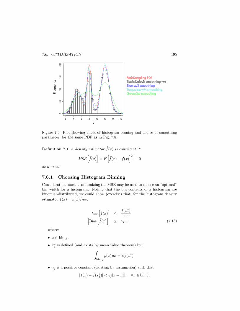
Red: Sampling PDFBlack: Default smoothing (w)Blue: w/2 smoothingTurquoise: w/4 smoothingGreen: 2w smoothing

Figure 7.9: Plot showing effect of histogram binning and choice of smoothingparameter, for the same PDF as in Fig. 7.8.

Definition 7.1 A density estimator f(x) is consistent if:

MSE[f(x)

]≡ E

[f(x)− f(x)

]2→ 0

as n→∞.

7.6.1 Choosing Histogram Binning

Considerations such as minimizing the MSE may be used to choose an “optimal”bin width for a histogram. Noting that the bin contents of a histogram arebinomial-distributed, we could show (exercise) that, for the histogram density

estimator f(x) = h(x)/nw:

Var[f(x)

]≤

f(x∗j )

nw∣∣∣Bias[f(x)

]∣∣∣ ≤ γjw, (7.13)

where:

• x ∈ bin j,

• x∗j is defined (and exists by mean value theorem) by:∫bin j

p(x) dx = wp(x∗j ),

• γj is a positive constant (existing by assumption) such that

|f(x)− f(x∗j )| < γj |x− x∗j |, ∀x ∈ bin j,


• equality is approached as the probability to be in bin j decreases (e.g.,by decreasing bin size).

Thus, we have a bound on the MSE for a histogram:

MSE[f(x)

]= E

[f(x)− p(x)

]2≤f(x∗j )

nw+ γ2jw

2.

Theorem 7.2 The MSE of the histogram estimator f(x) = h(x)/nw is con-sistent if the bin width w → 0 as n→∞ such that nw →∞.

Note that the w → 0 requirement insures that the bias will approach zero,according to our earlier discussion. The nw →∞ requirement ensures that thevariance asymptotically vanishes.

Theorem 7.3 The MSE(x) bound above is minimized when

w = w∗(x) =

[p(x∗j )

2γ2jn

]1/3.

This theorem suggests that the optimal bin size decreases as 1/n1/3. The1/n dependence of the variance is our familiar result for Poisson statistics. Theoptimal bin size depends on the value of the density in the bin. This suggestsan “adaptive binning” approach with variable bin sizes. However, accordingto Scott [4]: “. . . in practice there are no reliable algorithms for constructingadaptive histogram meshes.”

Alternatively, the MISE error is minimized (Gaussian kernel, asymptotically,for normally distributed data) when

w∗ =

(4

3

)1/5

σn−1/5.

An early and popular choice is Sturges’ rule, which says that the numberof bins should be

k = 1 + log2 n,

where n is the sample size. This is the rule that was used in making the his-togram in Fig. 7.8. It is the default choice when making a histogram in R.

However, the argument behind this rule has been criticized [3]. Indeed wesee in our example that we probably would have “by hand” selected more bins;our histogram is “over-smoothed”. There are other rules for optimizing thenumber of bins. For example, Scott’s rule [4] for the bin width is:

w = 3.5sn−1/3,

where s is the sample standard deviation. Physicists typically ignore theserules, and make explicit choices for the bin widths, often based on experimentalresolution. The standard rulesoften leave the visual impression that the binningcould usefully be finer, see Fig. 7.10.

7.7. THE CURSE OF DIMENSIONALITY 197D

ensi

ty

2 4 6 8 10 12 14 16

0.00

0.05

0.10

0.15

0.20

x

Red: Sampling PDF

Figure 7.10: Illustration of histogram binning. The red curve is the samplingPDF. The “standard rules” ( Sturges, Scott, Freedman-Diaconis) correspondroughly to the coarser binning above. The shaded histogram seems like a betterchoice.

7.7 The Curse of Dimensionality

While in principle problems with multiple dimensions in the sample space are notessentially different from a single dimension, there are very important practicaldifferences. This is referred to as the curse of dimensionality. The mostobvious difficulty is in displaying and visualizing as the number of dimensionsincreases. Typically one displays projections in lower dimensions, but this losesthe correlations that might be present in the un-displayed dimensions.

Another difficulty is that “all” the volume (of a bounded region) goes to theboundary (exponentially!) as the dimensions increases. This is illustrated inFig. 7.11. A unit cube in d dimensions is illustrated as d increases. A centralcube with edges 1/2 unit in length is shown. The fraction of the volume con-tained in this central cube decreases as 2−d. As a consequence, data becomes“sparse”. To obtain a suitable density of statistics, for example in a simula-tion tends to require exponentially growing computation as the dimensionalityincreases.

7.8 The Bootstrap

A statistical technique known as the bootstrap provides a means to evaluatehow much to trust our density estimate. The bootstrap algorithm in thiscontext is as follows:

1. Form density estimate p from data {xi; i = 1, . . . , n}.


1/2

1/41/8

, . . . 12d

Figure 7.11: Demonstration of the “curse of dimensionality”.

2. Resample (uniformly) n values from {xi; i = 1, . . . , n}, with replacement,obtaining {x∗i ; i = 1, . . . , n} (bootstrap data). Note that in resamplingwith replacement our bootstrap dataset may contain the same xi multipletimes.

3. Form density estimate p∗ from data {x∗i ; i = 1, . . . , n}.

4. Repeat steps 2&3 many (N) times to obtain a family of bootstrap densityestimates {p∗i ; i = 1, . . . , N}.

5. The distribution of p∗i about p mimics the distribution of p about p.

Consider, for a kernel density estimator, the expectation of the boostrapdataset:

E [p∗(x)] = E [K(x− x∗i ;w)] = p(x),

where the demonstration is left as an exercise. Thus, the bootstrap distributionabout p does not reproduce the bias which may be present in p about p.However, it does properly reproduce the variance of p, hence the bootstrap is auseful tool for estimating the variance of our density estimator. An illustrationof the distribution of bootstrap samples is shown in Fig. 7.12.

7.9 Estimating Bias: The Jackknife

We have seen that we may use the bootstrap to evaluate the variance of adensity estimator, but not the bias. Both properties are needed for a completeunderstanding of our estimator. A method that can be used to estimate biasis the jackknife. The idea behind this method is that bias depends on samplesize. If we can assume that the bias vanishes asymptotically, we may use thedata to estimate the dependence of the bias on sample size.

The jackknife algorithm is as follows:

1. Divide the data into k random disjoint subsamples.

2. Evaluate estimator for each subsample.

3. Compare average of estimates on subsamples with estimator based on fulldataset.

7.10. CROSS-VALIDATION 199

2 4 6 8 10 12 14 16

0001

002003

004Fr

equ

ency

x

Red: Sampling PDFRed: Sampling PDFBlack: Gaussian Kernel EstimatorBlack: Gaussian Kernel EstimatorOther colors: Resampled Kernel EstimatorsOther colors: Resampled Kernel Estimators

Figure 7.12: Use of the bootstrap to determine the spread of a Gaussian kerneldensity estimator.

Figure 7.13 illustrates the jackknife technique. Besides estimating the bias,jackknife techniques may also be used to reduce bias (see Scott [4]).

7.10 Cross-validation

Similar to the jackknife, but different in intent, is the cross-validation pro-cedure. In density estimation, cross-validation is used to optimize smoothingbandwidth selection. It can improve on “theoretical” optimizations by makinguse of the actual sampling distribution, via the available samples.

The basic method (“leave-one-out cross-validation”) is as follows: Form nsubsets of the dataset, each one leaving out a different datum. Use subscript−i to denote subset omitting datum xi. For density estimator f(x;w) evaluatethe following average over these subsets:

1

n

n∑i=1

∫f2−i(x) dx− 2

n

n∑i=1

f−i(xi).

The reader is encouraged to show that the expectation of this quantity is theMISE of f for n−1 samples, except for a term which is independent of w. Thus,we may evaluate the dependence of this quantity on smoothing parameter w,and select the value w∗ for which it is minimized. Figure 7.14 illustrates theprocedure.


Fre

quen

cy

2 4 6 8 10 12 14 16

010

020

030

040

0

x

Red: Sampling PDFHistogram: 2000 samplesBlack: Gaussian kernel estimatorOther Colors: Kernel jackknife estimators (each is on 500 samples; to be averaged together for jackknife)

Figure 7.13: Jackknife estimate of bias.

7.11 Adaptive Kernel Estimation

We saw in our discussion of histograms that it is probably more optimal to usevariable bin widths. This applies to other kernels as well. Indeed, the use ofa fixed smoothing parameter, deduced from all of the data introduces a non-local, hence parametric, aspect into the estimation. It is more consistent tolook for smoothing which depends on data locally. This is adaptive kernelestimation.

We argue that the more data there is in a region, the better that region can beestimated. Thus, in regions of high density, we should use narrower smoothing.In Poisson statistics (e.g., histogram binning), the relative uncertainty scales as

√N

N∝ 1√

p(x).

Thus, in the region containing xi, the smoothing parameter should be:

w(xi) = w∗/√p(xi).

There are two issues with implementing this:

• What is w∗?

• We don’t know p(x).

For p(x), we may try substituting our fixed kernel estimator, call it p0(x).For w∗, we use dimensional analysis:

D [w(xi)] = D[x]; D [p(x)] = D[1/x] ⇒ D[w∗] = D[√x]

= D[√σ].

7.12. MULTIVARIATE KERNEL ESTIMATION 201

0.2 0.4 0.6 0.8 1.0 1.2 1.4

−0.

125

−0.

120

−0.

115

−0.

110

−0.

105

−0.

100

w

Cro

ss V

alid

atio

n “

MIS

E”

w*

Choosing smoothing parameter whichminimizes estimated MISE.

0 5 10 150.

000.

050.

100.

150.

20

x

Pro

bab

ility

den

sity

Red: Actual PDFBlue: Kernel estimate, using smoothing from cross-validation optimizationDots: Kernel estimate with a default value for smoothing

Figure 7.14: Cross validation. Left: Determining the optimal w∗; Right: Ap-plying the optimized smoothing.

Then, for example, using the “MISE-optimized” choice earlier, we iterate on ourfixed kernel estimator to obtain:

p1(x) =1

n

n∑i=1

1

wiK

(x− xiwi

),

where

wi = w(xi) =

(4

3

)1/5√ρσ

p0(xi)n−1/5.

ρ is a factor which may be further optimized, or typically set to one.The iteration on the fixed-kernel estimator nearly removes the dependence

on our intitial choice of w. The boundaries pose some complication in carryingthis out.

There are packages for adaptive kernel estimation, for example, the KEYS(“Kernel Estimating Your Shapes”) package [5]. Figure 7.15 illustrates the useof this package.

7.12 Multivariate Kernel Estimation

Besides the curse of dimensionality, the multi-dimensional case introduces thecomplication of covariance. When using a product kernel, the local estimator


Figure 9 – Non-parametric p.d.f.s: Left: histogram of unbinned input data, Middle: Histogram-based p.d.f (2nd order interpolation), Right: KEYS p.d.f from original unbinned input data.

Figure 7.15: Example of the KEYS adaptive kernel estimation [6]

has diagonal covariance matrix. In principle, we could apply a local lineartransformation of the data to a coordinate system with diagonal covariancematrices. This amounts to a non-linear transfomation of the data in a globalsense, and may not be straightforward. However, we can at least work in thesystem for which the overall covariance matrix of the data is diagonal.

If {yi} is the suitably diagonalized data, the product fixed kernel estimatorin d dimensions is:

p0(y) =1

n

n∑i=1

d∏j=1

1

wjK

(y(j) − y(j)i

wj

) ,where y(j) denotes the j-th component of the vector y. The asymptotic, normalMISE-optimized smoothing parameters are now:

wj =

(4

d+ 2

)1/(d+4)

σjn−1/(d+4).

The corresponding adaptive kernel estimator follows the discussion as for theunivariate case. An issue in the scaling for the adaptive bandwidth arises whenthe multivariate data is approximately sampled from a lower dimensionalitythan the dimension d.

Fig. 7.16 shows an example in which the sampling distribution has diagonalcovariance matrix (locally and globally). Applying kernel estimation to this dis-tribution yields the results in Fig. 7.17, for two different smoothing parameters.

For comparison, Fig. 7.19 shows an example in which the sampling distribu-tion has non-diagonal covariance matrix. Applying the same kernel estimationto this distribution gives the results shown in Fig. 7.19. It may be observed(since this is the same data as in Fig. 7.16, just rotated to give a non-diagonalcovariance matrix) that this is more difficult to handle.

7.13. ESTIMATION USING ORTHOGONAL SERIES 203

4 6 8 10 12 14 16

24

68

1012

14

xy[,1]

xy[,2

]

Figure 7.16: A two-dimensional distribution with diagonal covariance matrix.

7.13 Estimation Using Orthogonal Series

We may take an alternative approach, and imagine expanding the PDF in aseries of orthogonal functions:

p(x) =

∞∑k=0

akψk(x),

where

ak =

∫ψk(x)p(x)ρ(x) dx = E [ψk(x)ρ(x)] ,

and ∫ψk(x)ψ`(x)ρ(x) dx = δk`,

where ρ(x) is a “weight function”.Since the expansion coefficients are expectation values of functions, it is

natural to substitute sample averages as estimators for them:

ak =1

n

n∑i=1

ψk(xi)ρ(xi),

and thus:

p(x) =

m∑k=1

akψk(x),


xy[1]

5

10

15xy[2]

5

10

Density function

0.000

0.005

0.010

0.015

0.020

xy[1]

5

10

15xy[2]

5

10

Density function

0.00

0.01

0.02

0.03

Figure 7.17: Kernel estimation applied to the two-dimensional data in Fig. 7.16.Left: Default smoothing parameter; Right: Using one-half of the defaultsmoothing parameter.

where the number of terms m is chosen by some optimization criterion.

Note the analogy between choosing m and choosing smoothing parameter win kernel estimators; and between choosing K and choosing {ψk}. We are actu-ally rather familiar with estimation using orthogonal series: It is the method ofmoments, or substitution method, that we described in Chapter 3. An exampleof an application of this method is shown in Fig. 7.20. In particular, the leftgraph shows the estimated spectra broken up by orthogonal function, in thiscase Y`m spherical harmonics.

7.14 Using Monte Carlo Models

We often build up a data model using Monte Carlo computations of differentprocesses, which are added together to get the complete model. This may involveweighting of events, if more effective time is simulated for some processes thanfor others. The overall simulated empirical density distribution is then:

f(x) =

n∑i=1

ρiδ(x− xi),

where∑ρi = 1 (or n to correspond with an event sample of some total size).

The weights must be included in computing the sample covariance matrix

7.15. UNFOLDING 205

−10

−5

05

1015

10 15 20 25 30 35 40

xy45[,1]

xy45[,2]

Figure 7.18: A two-dimensional distribution with non-diagonal covariance ma-trix.

(xi has components x(k)i , k = 1 . . . d):

Vk` =

n∑i=1

ρi(x

(k)i − µk)(x

(`)i − µ`)∑

j ρj,

where µk =∑

i ρix(k)i /

∑j ρj is the sample mean in dimension k.

Assuming we have transformed to a diagonal system using this covariancematrix, our product kernel density based on this simluation is then:

f0(x) =1∑j ρj

n∑i=1

ρi

d∏k=1

1

wkK

(x(k) − x(k)i

wk

).

This may be iterated to obtain an adaptive kernel estimator as discussed earlier.

7.15 Unfolding

We may not be satisfied with merely estimating the density from which oursample {xi} was drawn. The interesting physics may be obscured by convolutionwith uninteresting functions, for example efficiency dependencies or radiativecorrections. Thus, we wish to unfold the interesting distribution from thesampling distribution. Our treatment of this big subject will be cursory. See,for example, Ref. [8] for further discussion.


xy45[1]

−10−5

05

10

xy45[2]

10

15

20

25

30

35

Density function

0.000

0.001

0.002

0.003

0.004

0.005

xy45[1]

−10−5

05

10

xy45[2]

10

15

20

25

30

35

Density function

0.000

0.002

0.004

0.006

0.008

0.010

xy45[1]

−10−5

05

10

xy45[2]

10

15

20

25

30

35

Density function

0.000

0.002

0.004

0.006

0.008

Figure 7.19: Kernel estimation applied to the two-dimensional data in Fig. 7.18.Left: Default smoothing parameter; Middle: Using one-half of the defaultsmoothing parameter; Right: Intermediate smoothing.

We will assume the convolution function relating the two distribtuions isknown. However, it often is also estimated via auxillary measurements. Be-cause data fluctuates, unfolding usually also necessitates smoothing to controlfluctuations. This is referred to as Regularization in this context.

To set up a typical problem: Suppose we ample from a distribution withsome kernel function K(x, y):

o(x) =

∫K(x, y)f(y)dy.

We are given a sampling o, and wish to estimate f .In principle, the solution is easy:

f(y) =

∫K−1(y, x)o(x)dx,

where ∫K−1(x, y)K(y, x′) dy = δ(x− x′).

In practice, our observations are discrete, and we need to interpolate/smooth.If we don’t know how (or are too lazy) to invert K, we may try an iterative

solution. For example, consider the problem of unfolding radiative correctionsin a cross section measurement. The observed cross section, σE(s) is related tothe “interesting” cross section σ according to:

σE(s) = σ(s) + δσ(s),

where

δσ(s) =

∫K(s, s′)σ(s′) ds′.

7.15. UNFOLDING 207

Figure 7.20: The Kπ mass spectrum from Ref. [7]. Left: The measured spec-trum. The line histogram is the raw measurement data; the points show thedata corrected for acceptance. Left: The mass spectrum broken up by angulardistribution.


We form an iterative estimate for σ(s) according to:

σ0(s) = σE(s) (7.14)

σi(s) = σE(s)−∫K(s, s′)σi−1(s′) ds′, i = 1, 2, . . . (7.15)

Notice that this is just the Neumann series solution to an integral equation.Since σE(s) is measured at discrete s values and with some statistical preci-

sion, some smoothing/interpolation is still required.

7.15.1 Unfolding: Regularization

If we know K−1 we can incorporate the smoothing/interpolation more directly.We could use the techniques already described to form a smoothed estimate o,and then use the transformation K−1 to obtain the estimator f . For simplicity,consider here the problem of unfolding a histogram. Then we restate the earlierintegral formula as:

oi =

k∑j=1

Kijfj ,

where K is a square matrix, assumed invertible.A popular procedure is to form a likelihood (or χ2), but add an extra term,

a “regulator”, to impose smoothing. The modified likelihood is maximized toobtain the estimate for {fj}.

lnL → lnL′ = lnL+ wS(oi).

The regulator function S(oi) as usual gets its smoothing effect by being some-what non-local. A popular choice is to add a “curvature” term to be minimized(hence smoothed):

S(oi) = −k−1∑j=2

[(oi+1 − oi)− (oi − oi−1)]2.

This is implemented, for example, in the RUN package [9].Another implementation is GURU [10]. Further discussion may be found

in [11]. This paper has a nice demonstration of the importance of smoothing:Note that the transformation K itself corresponds to a sort of smoother, as itacts non-locally. The act of “unfolding” a smoother can produce large variances.

7.16 Non-parametric Regression

Regression is the problem of estimating the dependence of some “response”variable on a “predictor” variable. Given a dataset of predictor-response pairs{(xi, yi), i = 1, . . . , n}, we write the relationship as:

yi = r(xi) + εi,

7.17. SPLOTS 209

where the “error” εi might also depend on x through the parameters of thesampling distribution it represents.

We are used to solving this problem with parametric statistics, for example,the dependence of accelerator background on beam current, where we might trya power-law form. However, we may also bring our non-parametric methods tobear on this problem.

The sampling of the response-predictor pairs may be a fixed design inwhich the xi values are deliberately selected, or a random design, in which(xi, yi) is drawn from some joint PDF. We’ll work in the context of the randomdesign here, and also will work in two dimensions.

The regression function r may be expressed as:

r(x) = E [y|x] =

∫yp(y|x) dy =

∫yf(x, y) dy∫f(x, y)dy

.

Let us construct an estimator for r by substituting a bivariate product kernelestimator for the unknown PDF f(x, y):

f(x, y) =1

nwxwy

n∑i=1

K

(x− xiwx

)K

(y − yiwy

).

Assuming a symmetric kernel, after a little algebra we find:

r(x) =

n∑i=1

yiK

(x− xiwx

)/

n∑i=1

K

(x− xiwx

).

This is known as the local mean estimator. Note the absence of dependenceon wy, and the linearity in the yi.

We may achieve better properties by considering local polynomial estima-tors, corresponding to local polynomial fits to the data. This may be achievedwith a least-squares minimization (the local mean is the result for a fit to azero-order polynomial). Thus, the local linear regression estimate is given by:

r(x) =

n∑i=1

[S2(x)− S1(x)(xi − x)]K ((xi − x)/wx) yiS2(x)S0(x)− S1(x)2

,

where

S`(x) ≡n∑

i=1

(xi − x)`K

(x− xiwx

).

R provides a package loess for local polynomialregression fitting. Examplesof its use are shown in Figs; 7.21 and 7.22.

7.17 sPlots

The use of the density estimation technique known as sPlots [12] has gainedpopularity in some physics applications. This is a multivariate technique that


4 6 8 10 12 14 16

24

68

1012

14

xx

yy

−15 −10 −5 0 5 10 15

1015

2025

3035

xr45

yr45

Figure 7.21: Illustration of local linear regression using the loess package. Thedataset is the same in both plots, but the variables have been transformed by a45 degree rotation in the second plot. It may be observed that the introductionof covariance influences the result.

uses the distribution on a subset of variables to predict the distribution inanother subset. It is based on a (parametric) model in the predictor variables,with different categories (e.g., “signal” and “background”). It provides both ameans to visualize agreement with the model for each category and an easy wayto do “background subtraction”.

Assume there are a total of r + p parameters in the overall fit to the data:(i) The expected number of events, Nj , j = 1, . . . , r in each category, and (ii)Distribution parameters, {θi, i = 1, . . . , p}. We use a total of N events toestimate these parameters via a maximum likelihood fit to the sample {x}.

We wish to find weights wj(x′i), depending only on {x′} ⊆ {x} (and implicitly

on the unknown parameters), such that the asymptotic distribution in y /∈ {x′}of the weighted events is the sampling distribution in y, for any chosen categoryj. Assume that y and {x′} are statistically independent within each category.

The weights that satisfy our criterion and produce minimum variance summedover the histogram are given by [12]:

wj(e) =

∑rk=1 Vjkfk(x′e)∑rk=1 Nkfk(x′e)

,

where wj(e) is the weight for event e in category j V is the covariance matrixfrom a “reduced fit” (i.e., excluding y):

(V −1

)jk≡

N∑e=1

fj(x′e)fk(x′e)[∑r

i=1 Nifi(x′e)]2 ,

7.17. SPLOTS 211

1999 2000 2001 2002 2003 2004 2005

050

100

150

200

250

300

year

ndoc

8 10 12 14 16 18 20

6570

7580

85

diam

ht

Figure 7.22: Illustration of local linear regression using the loess package. Left:Applied to a dataset of cumulative publications from an experiment by year.The green lines just connect the dots. The other curves show the results forvariations on the regression. Right: Various regressions applied to a dataset oftree heights vs diameter (from R).

Nk is the estimate of the number of events in category k, according to thereduced fit. fj(x

′e) is the PDF for category j evaluated at x′e.

Finally, the sPlot is constructed by adding each event e with y = ye tothe y-histogram (or scatter plot, etc, if y is multivariate), with weight wj(e).The resulting histogram is then an estimator for the true distribution in yforcategory j. Figures 7.23 and 7.24 provide illustrations of the use of sPlots.

Typically the sPlot error in a bin is estimated simply according to the sumof the squares of the weights. This sometimes leads to visually misleadingimpressions, due to fluctuations on small statistics. If the plot is being madefor a distribution for which there is a prediction, then that distribution can beused to estimate the expected uncertainties, and these can be plotted. If theplot is being made for a distribution for which there is no prediction, it is moredifficult, but a (smoothed) estimate from the empirical distribution may be usedto estimate the expected errors.


0

5

10

15

20

-0.1 0 0.1

ΔE GeV

Eve

nts

/ 10

MeV

ΔEΔE

-10

0

10

20

30

-0.1 0 0.1

ΔE (GeV)

Figure 1. Signal distribution of the ΔE variable. The leftfigure is obtained applying a cut on the Likelihood ratio toenrich the data sample in signal events (about 60% of signalis kept). The right figure shows the sPlot for signal (all eventsare kept).

Figure 7.23: Illustration of the sPlot technique. Left: A non-sPlot, which uses asubset of the data in an attempt to display signal behavior. Right: An sPlot forthe signal category. The curve is the expected signal behavior. Note the excessof events at low values of ∆E. This turned out to be an unexpected portionof the signal distribution, which was found using the sPlot. From: M. Pivk,“sPlot: A Quick Introduction”, arXiv:physics/0602023 (2006).

7.17. SPLOTS 213

050

100150200

Events / 0.001 GeV/c2

K+π−π+γ

0

50

100

K+π−π0γ

0

20

40

KSπ−π+γ

5.200 5.225 5.250 5.275 5.300mES (GeV/c2)

0

20

40KSπ−π0γ

0.0

1.0

2.0

BF×106 / 0.02 GeV/c2

B+→K+π−π+γ

0.02.04.0 B0→K+π−π0γ

0.01.02.0

B0→K0π−π+γ

0.80 1.00 1.20 1.40 1.60 1.80mKππ (GeV/c2)

0.0

5.0

10.0 B+→K0π+π0γ

Figure 7.24: The sPlot technique used for background subtraction in mass spec-tra. Left: The spectra before background subtraction. Right: The spectra afterbackground subtraction using sPlots. From hep-ex/0507031.

Bibliography

[1] W.-M. Yao et al, J. Phys. G 33, 1 (2006).

[2] J. S. Halekas et al., “Magnetic Properties of Lunar Geologic Terranes:New Statistical Results”, Lunar and Planetary Science XXXIII (2002),1368.pdf)

[3] http://www-personal.buseco.monash.edu.au/∼hyndman/papers/sturges.pdf.

[4] David W. Scott, Multivariate Density Estimation, John Wiley & Sons, Inc.,New York (1992).

[5] K. S. Cranmer, “Kernel Estimation in High Energy Physics”,Comp. Phys. Comm. 136, 198 (2001) [hep-ex/0011057v1];http://arxiv.org/PS cache/hep-ex/pdf/0011/0011057.pdf;http://java.freehep.org/jcvslet/JCVSlet/diff/freehep/freehep/hep/aida/ref/pdf/NonParametricPdf.java/1.1/1.2.

[6] W. Verkerke and D. Kirkby, RooFit Users Manual V2.07:http://roofit.sourceforge.net/docs/RooFit Users Manual 2.07-29.pdf.

[7] G. Brandenburg et al., “Determination of the K∗(1800) Spin Parity”,SLAC-PUB-1670 (1975).

[8] Glen Cowan, “Statistical Data Analysis”, Oxford University Press (1998).

[9] V. Blobel, http://www.desy.de/∼blobel/wwwrunf.html.

[10] A. Hocker & V. Kartvelishvili, “GURU”, NIM A bf 372, 469 (1996).

[11] Glen Cowan, http://www.ippp.dur.ac.uk/Workshops/02/statistics/proceedings//cowan.pdf.

[12] M. Pivk & F. R. Le Diberder, “sPlot: a statistical tool to unfold datadistributions”, Nucl. Instr. Meth. A 555, 356 (2005).

215

density estimation - caltech high energy physicsfcp/statistics/densityest/densityest.pdf · density...

Documents