density-dependent migration and stability in a system of linked populations

Bulletin of Mathematical Biolog),, Vol. 58, No. 4, pp. 643-660, 1996 Elsevier Science Inc.

�9 1996 Society for Mathematical Biology 0092-8240/96 $15.00 + 0.00

0092-8240(95)00362-2

DENSITY-DEPENDENT MIGRATION AND STABILITY IN A SYSTEM OF LINKED POPULATIONS

G R A E M E D. R U X T O N Division o f Envi ronmenta l and Evolut ionary Biology,

�9 Insti tute of Biomedical and Life Sciences, University of Glasgow Glasgow G12 8QQ, Uni ted Kingdom

(E.mail: g.ruxton.bio.gla.ac.uk)

The effect of adding density-dependent migration between nearest neighbour populations of a single discrete-generation species in a chain of habitat fragments is investigated. The larger the population on a particular habitat fragment, the greater the fraction of inhabi- tants who migrate before reproducing. It has previously been shown for similar models with density-independent migration that coupling populations in this way has no effect on the stability of these populations. Here, it is demonstrated that this effect is also generally true if migration is density-dependent. However, if the migration rate is large enough and has density dependence of the correct form, then the steady state (with all the populations remaining at the same constant value through time) can be destabilised. The conditions for this to occur are obtained analytically. When this "destabilisation" occurs, the system settles down to an alternative steady state where half of the populations take one constant value which is below that of an equivalent isolated system, and the other populations all share a population value which is greater than the steady state of the isolated populations. Once this configuration is reached, the population size on each patch remains constant over time. Hence the change might more properly be described as a decrease in homogeneity rather than in stability.

1. Introduction. Within the past decade there has been a growing interest in the role of space in determining population dynamics (see Taylor, 1990, Renshaw, 1991, and Gilpin and Hanski, 1991, for useful overviews). One fundamental question which has received a great deal of attention is the population dynamic effects of migration between populations which are separated in space (see Bascompte and So16, 1995a, for a recent review). In such studies, the changes in population sizes over space and time are often represented using so-called "coupled map lattices" (CMLs). These models assume that births and deaths within individual populations are described by difference equation models (see May (1973) and Hassell (1975) for a full

643

644 G . D . RUXTON

discussion of these). In addition, however, they allow individuals to move between populations. By far, the most common rule adopted is that a fixed fraction of the individuals on each site migrate at each generation (Gonzhlez-Andfljar and Perry 1993a, b; Hastings, 1993; Gyllenberg et al., 1993; Bascompte and So16, 1994; Lloyd, 1995; Doebeli, 1995), distributing themselves among the other sites according to some density-independent rule. One particularly important recent development in this theory is presented in the papers of Hassell et al. (1995) and (more fully in) Rohani et al. (1996), which demonstrate analytically that such density-independent coupling has no effect on whether the steady states of a variety of commonly used models will be locally stable or unstable.

In contrast to the foregoing density-independent case, the effect of density-dependent migration has not received much attention. This seems particularly strange because all the studies previously discussed assume that either reproduction or mortality has a density-dependent component. It is easy to imagine situations which lead to density-dependent migration rates. For example, individuals may be more likely to leave a population which has fallen to a very low value because of the poor choice of mates or because collective defensive or foraging behaviours are compromised by the low population size. At the opposite extreme, one could expect individuals to have an increased propensity toward migration if their current population is very large because competition for resources, such as food or breeding sites, may be very high. This paper will consider the second case, where the per capita migration rate out of a population increases with the size of that population, and will examine the effect which this has on the stability of the steady state.

There is some evidence to suggest that introducing density dependence to migration may have significant effects on population dynamics. Csilling et al. (1994) examined a CML model similar to that investigated by Bascompte and So16 (1994), but found quite different behaviour. One novel feature of the model of Csilling et al. was the use of a crude form of density dependence in migration through the use of a threshold population value: populations which fall below this value suffer no loss through migration. However, this evidence is far from conclusive, especially since Csilling et al. also introduce a novel rule about the relative timing of migration and reproduction events. This has lead to some debate about the relative importance of these two mechanisms in affecting the dynamics of the model (Hastings and Higgins, 1995; Paradis, 1995; Ruxton, 1995). The aim of this paper is to investigate the role of density-dependent migration in the absence of other confounding factors. The next section sets out a simple CML on which this investigation will be based.

M I G R A T I O N AND STABILITY IN LINKED POPULATIONS 645

2. The Model. Consider a linear collection of N habitat fragments. Each of these fragments holds a population of a single species with discrete generations. The species is considered to have two important life stages called juvenile and adult. At a given generation (t ~ {0, 1, 2,... }), the size of the adult population of a specific fragment (i ~ {1, 2, . . . , N}) is denoted A~. The size of the equivalent juvenile population is denoted Ji t.

We define the division between generations so that the population at the end of a generation ( t , say) consists wholly of juveniles. At the start of the next generation, a fraction, 0 < ~)(Ji t) ~ 1, leave their current population for another, and then all juveniles mature into adults. The N populations are arranged serially and the migrants from each population are added to the populations immediately before and after their original site, being divided equally between the two. To avoid boundary effects, the boundary conditions are periodic so that the Nth population is neighboured by the ( N - 1 ) t h and the first. This can be envisaged as the end patches being joined so that the line forms a continuous ring. Defining the number of migrants leaving patch i at the start of generation t + 1 as M[ + 1, then clearly

M/+ l = 4k( Jit)4t. (1)

After immigration, the adult populations on each patch are given by

At l+I=(J~-M~+I) +O.5M~ +1 + 0 . 5 M ~ + 1 , (2)

A ~ + l = ( J i t - M t + l ) + O ' 5 M t - + l + ~ 1 ' i ~ {2, N - 1} , (3)

At f f 1 = [ r t Art+ 1 ~ 0 5 M t+ 1 0.5M[+ 1. I,~'N - - ~ '*N ] -{- �9 N - 1 -'1- (4)

The fraction of the juveniles alive in population i at the end of generation t who will migrate at the start of generation t + 1 is given by

dp( Jit) = q~max(1- e x p ( - "yJit) ), (5)

where ~bma x is the maximum fraction of any population that can migrate in any given generation (0 < ~bma x < 1) and Y controls the strength of the density dependence. In the limit y-~ % c~(Ji t) ~ ~bma x and there is no density dependence. However, at lower values of y, c~(Ji t) increases with population density.

After the migration stage, reproduction occurs to produce a juvenile population on each habitat fragment. The number of juveniles produced is

646 G . D . R U X T O N

a simple function of the number of adults on the patch after the migration process:

j[+l =Ati+lF(Ati+l). (6)

After the reproductive stage, the adults die, leaving the new juvenile populations at the end of the generation. The function used to represent the per capita production of juveniles is

F ( A ) = A(1 + a A ) -t3, (7)

where A, a and /3 are all positive and are constant both over time and between patches, h is the maximum number of offspring that can be produced, a is the inverse of the carrying capacity of any given patch and/3 controls the strength of the density dependence in reproduction.

This function has been used in many other similar studies (e.g., Bascompte and So16, 1994; Csilling et al., 1994; Hassell et al., 1995). A full description of the behaviour of this model for a single population can be found in Hassell (1975) and Hassell et al. (1976).

3. A Single Isolated Population. For comparison purposes, we briefly consider the behaviour of a single population governed by

A t+l = hAt(1 + aAt ) -t~. (8)

This can be seen as the limit 4'm~ ~ 0 of the full model. Setting A t+ 1 = A t ----~zl, it is trivial to show that the non-zero steady state

is given by

A 1 / / 3 - - 1 A - , (9)

O~

which is non-negative providing h > 1. Hassell (1975) shows that this steady state is locally stable providing

0 < 2 where

0=/3(1 - l ~ - l / fl ) . (10)

The behaviour of the population for various values of /3 is summarised in Fig. 1. At low/3, the equilibrium is stable. At the critical value predicted by equation (10), a bifurcation occurs, the steady state becomes locally unstable and the population performs a two point cycle. As /3 is increased

MIGRATION AND STABILITY IN LINKED POPULATIONS 647

500

4OO

"•'• 300 r

" 0 c - O

200 Q . 0 EL

100

\ .

02 4 6 8 10

Figure 1. A bifurcation diagram describing the population dynamics of a single population described by equation (8). For each value of /3, the population is initialised to take a value randomly drawn from a uniform distribution on [0, 1/a]. The population is then iterated through 400 generations, to remove transient effects, before the value of the population at each of the next 50 generations is plotted against /3. If, for a particular/3 value, the steady state is stable, each of the population values plotted will be identical and so only a single point will be seen of the plot. Similarly, if the steady state is unstable and the population is performing an n-point cycle, then n distinct points will be observed. If a large number of points are observed for a particular /3 value, then this is suggestive of aperiodic behaviour such as chaos. Other parameters: a = 0.01, A = 30.

fur ther , so the size of the oscil lat ion grows unti l (at /3 = 5.7 in Fig. 1) the system bifurcates again to a four point cycle. Fu r t h e r bi furcat ions occur with progressively smaller increases in /3, unti l finally chaos can be observed. This can be seen f o r / 3 values grea ter than 7.7 in Fig. 1, a l though there is a window of simple per iodic behav iour a round /3 = 8.8.

4. A Network of Populations. Append ix 1 describes the local stability analysis for the ne twork of l inked popula t ions and calculates tha t the s teady state where all pa tches have a popu la t ion of size A is stable if and only if

0 (1- )expt- <1

648 G .D . RUXTON

and

I1 - OI < 1. ( 1 2 )

The second condition is identical to that for a single population to be stable. Hence, we can see that migration cannot stabilise the dynamics of populations which would be unstable in the absence of migration. We now ask under what circumstances can migration destabilise dynamics.

In the limit ~, --+ % th(L t) --+ t~max and there is no density dependence in the migration term. In this limit, the first stability condition simplifies to

[ ( 1 - 0 ) ( 1 - 24~max)l < 1. (13)

Since 0 < thmax < 1, this is more restrictive than the stability condition for the isolated population. Hence parameters which satisfy the second stability condition (equation (12)), will certainly satisfy the first (equation (11)). Hence, in this limit, the stability condition of the linked network is identical to that of an isolated population, in agreement with the findings of Rohani et al. (1996).

We now investigate the effect of allowing density dependence into the migration term. A necessary condition for density-dependent migration to destabilise the steady state is

I (1- 3,d)exp(-3,d))<1. (14)

For demonstration purposes, we define

Y= (1 - (1 - 3 ,d)exp(- ~/d)) (15)

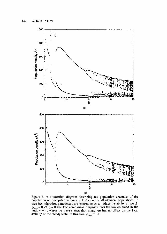
and plot this as a function of (yA') in Fig. 2. Elementary calculus shows that Y is bounded below by 0.0 and above by 1.135. Recalling that (0 < ~bma , < 1), it is clear that condition (14) can be satisfied but only when ~bma ~ is very high (at least above 0.88). Satisfying condition (14) is necessary but not sufficient to guarantee instability; it can, however, drive the system unstable providing that parameters are chosen so that 0 is slightly less than 2.0. Figure 3a shows an example of this effect; the intrinsic growth parameters are the same as those used to produce Fig. 1. The migration parameters are chosen to produce a strong destabilising effect: the maximum migration rate is high (~bm~ x = 0.99) and the density dependence in migration is very strong (y = 0.009). For comparison purposes, Fig. 3b shows the same system in the limit 3' --+ % where there is no density dependence in migration.


1.5

1.0

0.5

0.0 i I I i I I

2 4 6 8 10

Figure 2. Plot of Y (defined in equation (15)) against the product of the steady state population density A and the density-dependence constant 3'. Y being greater than 1 is a necessary condition for instability. The larger Y is, the more likely it is that such instability occurs.

However, bifurcation diagrams like those shown in Fig. 3 can be mislead- ing. In the system without density dependence (Fig. 3b) the instability which occurs beyond/3 values around 3.0 causes each population to exhibit a two point cycle. That is, the population oscillates between two values, taking alternate values in consecutive generations. The coupling also acts to synchronise the populations so that they all take the same value in any given generation. This situation is illustrated in Fig. 4a. The "new" instability which occurs below /3 values of 3.0 in Fig. 3a looks similar in the bifurcation diagram, but is in fact quite different. The instability induced by the density dependence in migration causes populations to alternate between two values along the line of populations, neighbouring populations taking on different values. However, the population in any one patch remains unchanged from one generation to the next. This situation is illustrated in Fig. 4b. Bifurcation diagrams like Fig. 3a are generated from many simulations (one for each /3 value), each with random initial conditions. Some initial conditions cause the system to organise so that patch 1, say, takes the higher of the two possible values; other initial conditions will cause it to take the lower value. For this reason, it looks superficially as if the population is undergoing a two point cycle, whereas in fact, the

500

400

"•'• 300 t . . -

"0

o .~ 200 Q. o 0..

100

0 2

500

i . .

4 6 8 10

(a)

650 G . D . RUXTON

400

aoo U'b

~ "o

o 200

D.,

= ;. . 10o "'-;<:

2 4 6 8 10 P

(b)

Figure 3. A bifurcation diagram describing the population dynamics of the population on one patch within a linked chain of 20 identical populations. In part (a), migration parameters are chosen so as to induce instability at low/3: ~bma x = 0.99, 3' = 0.009. For comparison purposes, part (b) was obtained in the limit ~/--* o0 where we have shown that migration has no effect on the local stability of the steady state, in this case 4~m~x = 0.l.


(a)

(b) Figure 4. Time series showing the population density in each of 20 linked patches in each of 50 successive generations. Population densities greater than or less than 200 are represented by dark or light squares, respectively. In part (a)/3 = 3.2, so that the system is in the region of parameter space where isolated populations would exhibit a two-point cycle through time. The two-point cycle is preserved in the linked system and all the populations change in phase, so that at any point in time, each patch has the same population density. In part (b), /3 = 2.8, so that the populations undergo the new instability induced by the density-dependent migration. It can be seen that the density in each patch remains constant over time. However, neighbouring patches have different population densities: odd numbered patches 98.7 and even numbered patches 467.9. Other parameters: c~ = 0.01, A = 30, ~max = 0.99, y = 0.009.

652 G . D . RUXTON

population in patch 1 (and in all the patches) settles to one time-invariant value. The instability for /3 values above 3.0 is unaffected by this density dependence and is of the same form as that illustrated in Fig. 4a.

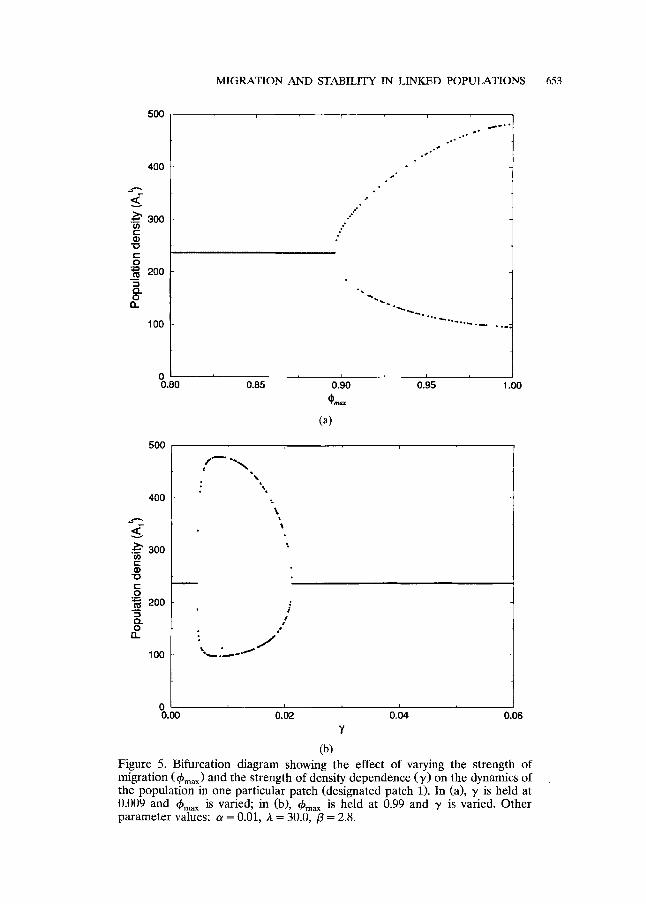
As emphasised by the investigation of the eigenvalues, this density- dependence-induced instability can only be achieved if the number of individuals migrating each generation is very high. This is illustrated by the bifurcation diagram in Fig. 5a which shows the effect of varying migration for one particular/3 value (2.8) in the system studied in Fig. 3a. Figure 5b demonstrates that the density dependence must be neither too strong nor too weak if the "new" instability is to be induced. The shape of the migration term for several values of 7 is shown in Fig. 6.

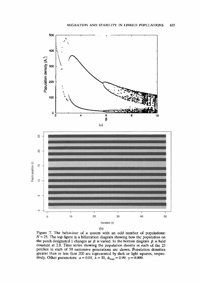
The analytical investigation of the eigenvalues presented earlier made the assumption that the number of habitat patches in the system was even. However, the qualitative conclusions of this work are unchanged if an odd number of patches is considered (compare Fig. 7a with Fig. 3a). The only difference which emerges is that if the number of patches is odd, then, if the "new" instability occurs, two neighbouring patches will take the same value. In all other cases, neighbouring patches take opposite values, as illustrated in Fig. 7b. The position of the two neighbours which take the same values is determined by the initial population values across the whole system.

Another generalisation of the theory would be to investigate the effect of changing the boundary conditions from periodic to absorbing. In this case the two end populations are no longer coupled by migration; instead haft of the migrants from both of these two populations are lost from the system. Rohani et al. (1995) suggested that stability is unaffected by this change providing the system size is large (as illustrated in Fig. 8a). It would appear that the effect of density-dependent migration is similarly unaffected (as illustrated in Fig. 8b).

5. Discussion. The main conclusion of this study is that, at least for the system under study, there is a strong suggestion that density-dependent migration has little effect on the local stability of the equilibrium of the system. Previously, Rohani et al. demonstrated for a variety of coupled map lattices that density-independent migration had no effect on local stability. Bascompte and So16 (1995b) suggest that Rohani et al.'s results are relevant only to a few natural species since they are all based on models where migration and reproduction occur in discrete and non-overlapping intervals within each generation. The same assumption is made in the model used in this study. However, Ruxton (1996) describes the analysis of a model similar to that used here, but which relaxes the segregation of migration and

500

400

300 r t "

" 0 c- O

200

O_ 0

Q.

100

0 0.81

500


..-'" ~

~ 0 ,~176

~176

~ ~ q ~ e g ~ i ~ I O m

i i i

0.85 0,90 0.95 (•)•

(a)

1.00

400

300 t-

nO

t-

O .~ 200

0 - 0

100

%

"t t

I , i

.00 0.02 0.04 0.06

7

(b) Figure 5. Bifurcation diagram showing the effect of varying the strength of migration (~bma x) and the strength of density dependence (30 on the dynamics of the population in one particular patch (designated patch 1). In (a), T is held at 0.009 and ~bm~ is varied; in (b), ~bma ~ is held at 0.99 and T is varied. Other parameter values: a = 0.01, A = 30.0, /3 = 2.8.

654 G.D. RUXTON

1.0

" ~ 0.8

"~ 0.6 8_ :5

t / )

0.4

0.2

i I I i I i I

o.o o loo 200 300 400 soo Population density (/~t)

Figure 6. Diagram illustrating the effect which varying the strength of the density-dependence constant (7) has on the fraction of migrants leaving a patch. The density of migrants leaving a patch M[ was obtained from equation (1) and was then scaled by the population density (A~) to obtain the fraction migrating. This is then expressed as a proportion of the maximum fraction which can ever migrate (~bma~). This proportion is then calculated for a range of possible population densities for three values of 3': 0.001, 0.01 and 0.1. With 7 = 0.1, the graph rapidly saturates and the fraction is effectively 1.0 for all population values above 100. As 3' is reduced, so the fraction migrating at any particular population density is also reduced. At the opposite extreme, when 3' = 0.001, the fraction migrating is still below 0.4, even when the population climbs to very high values.

reproduction and finds, once again, that migration has little effect on local stability.

There have been some studies of linked populations which found that simple density-independent migration could be destabilising. In a recent paper, Bascompte and So16 (1994) investigated the effects of local dispersal on the dynamics of discrete-generation populations using a CML. They found that as the rate of diffusion (D) is increased, "there is a well defined bifurcation scenario in which chaos beyond a characteristic D-value is reached." If the uncoupled populations exhibited equilibrium state or cyclic behaviour, then the addition of only modest amounts of migration between local populations induced a series of period-doubling bifurcations leading to chaos. Hassell et al. (1995) re-examined the model of Bascompte and So16 (1994) and suggested that the model's formulation "fails to segregate


500

4OO

' "

g _ 200

loo ".'\ "c=~

o 2 4 6 8 10

(a)

(b) Figure 1. The behaviour of a system with an odd number of populations: N--- 25. The top figure is a bifurcation diagram showing how the population on the patch designated 1 changes as /3 is varied. In the bottom diagram /3 is held constant at 2.8. Time series showing the population density in each of the 25 patches in each of 50 successive generations are shown. Population densities greater than or less than 200 are represented by dark or light squares, respectively. Other parameters: a = 0.01, h = 30, ~max = 0.99, 3' = 0.009.

656 G . D . R U X T O N

500

400

o o

._~ 300

C

" 0 r

o 200

Q . 0

Q . .

IO0

0 2

I i I

3 4

P (a)

500

400

<~ ._.~ 300 f./) t ' - O~

" 0 (...

._o 200

"1 0 . . 0

0 . .

100

\ .

%~

" < i ~ 1 7 6

I I I

0 3 4 5

P (b)

Figure 8. Bifurcation diagram showing the population dynamics of a population in the centre of a line of 200 populations. Now dissipative boundary conditions are used, where half of the migrants from the two end populations are lost from the system. In (a) there is no density dependence in the migration term (7 ~ oo); in (b), 7 = 0.009. Other parameter values: a = 0.01, A = 30, (])max = 0.99.


the processes of survival and dispersal. As a result, the same individual can fail to survive and yet disperse. At its most extreme, this leads to the production of negative local population densities." Reeve (1988) studied a system of linked host-parasitoid interactions, where migrants from both species join "pools" which are then divided evenly throughout the system. He found that if migration was strongly asymmetric, with one species having a strong tendency to migrate and the other a very weak one, then the linked system could display cyclic oscillations when an unlinked (non- spatial) interaction settled to a stable equilibrium. He suggested that this effect is produced by the effective decoupling of the population densities in any given patch because of the strong asymmetry in migration. Rohani et al. (1995), however, argued that asymmetry in dispersal, no matter how pro- nounced, does not cause such instabilities in the models they analysed.

One assumption of my model, and indeed all those discussed so far, is that, although species under investigation are distributed through space, they are distributed in such a way that the system can be considered as a finite number of discrete metapopulations. In effect, the species exist in a finite number of island habitat patches in a sea of unsuitable habitat. This is often an idealisation of real populations. In the opposite extreme, we could consider the species to be continuously distributed across some spatial domain in such a way that subpopulations cannot be identified. Such systems have long been studied in population ecology (see Okubo, 1980, and Murray, 1989, for overviews). In this case, spatial movement of individuals frequently leads to instabilities. Good examples of this effect have been demonstrated by Pascual (1993) and Neubert et al. (1995). As empha- sized earlier, continuous space and metapopulation models are two ex- tremes which bracket the actual spatial behaviour of natural species. Since the effect of movement seems so different in these two limits, there is a pressing need to explore the middle ground between these two situations.

Even in the metapopulation case, where subpopulations can be identified, although this study adds weight to the suggestion that migration may often have no effect on local stability, this should not be interpreted as the suggestion that it has no consequence to the structure and behaviour of ecological systems. Such migration can allow persistence of the system as a whole despite the frequent local extinction of subpopulations, as demonstrated by Hassell et al. (1991). For competing species, local dispersal between subpopulations can allow co-existence which would not be possible otherwise (Hassell et al., 1994). In fact, it is the relative importance of migration in real ecological situations which should drive us to further efforts to understand the subtleties of its effects.

I thank two anonymous referees for helpful comments.

658 G. D. RUXTON

APPENDIX

Local Stability Analysis.

1. Population network. We have a system of N populations governed by

A~+I = j/t _ gbmax j/t (1 _ exp( - y g ) ) + 0.5(;bm.x Ji t_ 1(1 - exp( - yJi t_ ,))

+ 0.5q~maxJ/t 1(1 - e x p ( - y J/+ 1)), (A1)

j[+ l = AA~+ iF(A~+ I), (A2)

where i : = 1,2 . . . . . N, JO=JN and JN+a =Jr We perturb the system slightly from equilibrium:

Ji =.d + xi, (A3)

Ai ='4 + Yi. (A4)

We substitute in these values, use Taylor expansion and discard all terms other than those linear in the perturbations.

The resulting equations can be represented in matrix form

xt+l =/~t, (A5)

where x t+ 1 and x t are column vectors of length N and A is an N • N matrix of the form

A =

a b 0 ... 0 b - ]

1 b a b 0 "" 0 0 b a b 0 0

0 ... 0 b a b b 0 . " 0 b a

(A6)

where

a = (1 - 0)(1 - ~max + ~maxeXp( -yA)[1 + y A ] ) , (A7)

b = 0.5(1 - O)q~max(1 -- exp( -- yA)[1 - yA]) . (AS)

The system is locally stable, that is, the perturbations die away, if and only if all the eigenvalues of this matrix have modulus less than 1.

If N is even, then from May (1973, pp. 197-199), the N eigenvalues of this matrix are given by

E ~=a+2bcos (~ - -~ ) , (A9)

where k = 0, 1 , . . . , N - 1.


The formula is slightly more complex if N is odd. We only consider the even case here since there is little difference between the eigenvalues for system sizes N and N - 1, and these differences decrease in magnitude as N is increased.

The biggest eigenvalue will occur when the cosine takes an extreme value, i.e. when k = 0 or N/2:

E o = (1 - O) (AIO)

EN/2 = (1 -- 0)(1 -- [26max(1 -- (1 -- yA)exp( -yA) ) ] ) . (Al l )

Hence the conditions for stability are

IEN/21 < 1, 11 -- 01 < 1. (A12)

REFERENCES

Bascompte, J. and R. V. Sol& 1994. Spatially induced bifurcations in single-species population dynamics. J. Anim. Ecol. 63, 256-264.

Bascompte, J. and R. V. So16. 1995a. Rethinking complexity: modelling spatiotemporal dynamics in ecology. Trends Ecol. Evol. 10, 361-365.

Bascompte, J. and R. V. So16. 1995b. Appropriate formulations for dispersal in spatially structured models: reply. J. Anita. Ecol. 64, 665-666.

Csilling, A., I. M. Janosi, G. Pasztor and I. Scheuring. 1994. Absence of chaos in a self-organised critical coupled map lattice. Phys. Rev. E 50, 1083-1092.

Doebeli, M. 1995. Dispersal and dynamics. Theoret. Population Biol. 47, 82-106. Gilpin, M. and I. Hanski. 1991. Metapopulation Dynamics: Empirical and Theoretical Investi-

gations. London: Academic Press. Gonzfilez-Andfljar, J. L. and J. N. Perry. 1993a. The effect of dispersal between chaotic and

non-chaotic populations within a metapopulation. Oikos 66, 555-557. Gonzfilez-Andfijar, J. L. and J. N. Perry. 1993b. Chaos, metapopulations and dispersal.

Ecological Modelling 65, 255-263. Gyllenberg, M., S. Gunnar and S. Ericsson. 1993. Does migration stabilize population

dynamics? Analysis of a discrete metapopulation model. Math. Biosci. 118, 25-49. Hassell, M. P. 1975. Density-dependence in single-species populations. J. Anim. Ecol. 44,

283-295. Hassell, M. P., J. H. Lawton and R. M. May. 1976. Patterns of dynamical behaviour in single

species populations. J. Anim. Ecol. 45, 471-489. Hassell, M. P., H. N. Comins and R. M. May. 1991. Spatial structure and chaos in insect

population dynamics. Nature 353, 255-258. Hassell, M. P., H. N. Comins and R. M. May. 1994. Species coexistence and self-organising

spatial dynamics. Nature 370, 290-292. Hassell, M. P., O. Miramontes, P. Rohani and R. M. May. 1995. Appropriate formulations

for dispersal in spatially structured models: reply to Bascompte and Sol& J. Anim. Ecol. 64, 662-664.

Hastings, A. 1993. Complex interactions between dispersal and dynamics: lessons from coupled logistic equations. Ecology 74, 1362-1372.

Hastings, A. and K. Higgins. 1995. Chaos and scale. Trends Evol. Ecol. 10, 335. Lloyd, A. L. 1995. The coupled logistic map: a simple model for the effects of spatial

heterogeneity on population dynamics. J. Theor. Biol. 173, 217-230. May, R. M. 1973. Stability and Complexity in Model Ecosystems. Princeton: Princeton

University Press.

660 G.D. RUXTON

Murray, J. D. 1989. Mathematical Biology. Berlin: Springer-Verlag. Neubert, M. G., M. Kot and M. A. Lewis. 1995. Dispersal and pattern formation in a

discrete-time predator-prey model. Theoret. Population Biol. 48, 7-43. Nisbet, R. M. and W. S. C. Gurney. !982. Modelling Fluctuating Populations. Chichester:

Wiley. Okubo, A. 1980. Diffusion and Ecological Problems: Mathematical Models. Berlin: Springer-

Verlag. Paradis, E. 1995. Chaos and scale. Trends. Ecol. Evol. 10, 335. Pascual, M. 1993. Diffusion-induced chaos in a spatial predator-prey system. Proc. Roy.

Soc. London Ser. B 251, 1-7. Reeve, J. D. 1988. Environmental variability, migration and persistence in host-parasitoid

systems. Am. Nat. 132, 810-836. Renshaw, E. 1991. Modelling Biological Populations in Space and Time. Cambridge: Cam-

bridge University Press. Rohani, P., R. M. May and M. P. Hassell. 1996. Metapopulations and local stability: the

effects of spatial structure. J. Theor. Biol., in press. Ruxton, G. D. 1995. Chaos and scale. Trends Ecol. Euol. 10, 335-336. Ruxton, G. D. 1996. Dispersal and chaos in spatially structured models: an individual-level

approach. J. Anim. Ecol., in press. Taylor, A. D. 1990. Metapopulations, dispersal and predator-prey dynamics: an overview.

Ecology 71, 429-443.

R e c e i v e d 28 A u g u s t 1995

density-dependent migration and stability in a system of linked populations

Documents