dense and sparse labeling with multi dimensional features
TRANSCRIPT

Copyright © 2016 IEEE. Personal use of this material is permitted. However, permission to use this material for any other purposes must be obtained from the IEEE by sending an email to [email protected].
Abstract—Conventional low-level feature based saliency
detection methods tend to use non-robust prior knowledge and do
not perform well in complex or low-contrast images. In this paper,
to address the issues above in existing methods, we propose a
novel deep neural network (DNN) based dense and sparse labeling
(DSL) framework for saliency detection. DSL consists of three
major steps, namely dense labeling (DL), sparse labeling (SL) and
deep convolutional (DC) network. The DL and SL steps conduct
initial saliency estimations with macro object contours and
low-level image features, respectively, which effectively
approximate the location of the salient object and generate
accurate guidance channels for the DC step; the DC step, on the
other hand, takes in the results of DL and SL, establishes a
6-channeled input data structure (including local superpixel
information), and conducts accurate final saliency classification.
Our DSL framework exploits the saliency estimation guidance
from both macro object contours and local low-level features, as
well as utilizing the DNN for high-level saliency feature extraction.
Extensive experiments are conducted on six well-recognized
public datasets against sixteen state-of-the-art saliency detection
methods, including ten conventional feature based methods and
six learning based methods. The results demonstrate the superior
performance of DSL on various challenging cases in terms of both
accuracy and robustness.
Index Terms—Saliency detection, deep neural network, dense
labeling, sparse labeling, macro object contour, low-level feature
I. INTRODUCTION
ALIENCY detection, which originates from the contrast
detection of human visual system [3], has experienced
drastic developments in the researches of computer vision in
recent years. Its ultimate goal is to mimic the intrinsic functions
of human visual system, by which the understanding of the
surrounding environment can be conducted accurately and
effortlessly. Since emergence, saliency detection is functioning
as an important preprocessing step in computer vision, which is
widely applied in various image analysis tasks such as image
segmentation [4], object detection [5], [6], object tracking [7],
picture collaging [8], [9], and color filtering [10], [11], etc.
Early researches of saliency detection mostly focus on
human eye fixation [3], [12], [13], which approximates the
visual attention of semantic objects in a given image, such as
human faces, texts, or daily objects [12], [14]. The detection
results of eye fixations, however, are often presented as sparse
dots without details about the objects. On the other hand, the
recently emerged salient object detection is capable of locating
and segmenting the whole salient object with complete
boundary details [15], and hence has received broad research
interests.
Salient object detection (or simply saliency detection) aims
to locate the most informative and attention-catching object in
an image [16]. To achieve such objective, an intuitive way is to
take advantage of the low-level features within the input image
itself, which is the core idea of most conventional saliency
detection methods. These features include but are not limited to:
color [3], [13], histogram [17], [18], spatial distribution [19],
[20], color filter response [10], [11], spectrum [21], [22], data
architecture [1], [23], and background prior [24], [25], etc.
These low-level feature based saliency detection methods are
usually efficient to conduct, since no training process is
involved. They have shown promising results both in
bottom-up approaches [21], [26-30] and in top-down
approaches [18], [31], [32]. Nevertheless, at least three major
drawbacks hinder their performances: (1) Without feature
abstraction and learning, their hand-crafted low-level features
are only effective on relatively high contrast images and do not
perform well on images with complex foreground / background
contexts. This drawback, however, can be readily solved via
high-level feature learning, which is seen in Fig. 1a. (2) Most of
the prior knowledge applied in low-level feature based methods
Dense and Sparse Labeling with
Multi-Dimensional Features for Saliency Detection
Yuchen Yuan, Student Member, IEEE, Changyang Li, Member, IEEE, Jinman Kim, Member, IEEE,
Weidong Cai, Member, IEEE, and David Dagan Feng, Fellow, IEEE
S
Fig. 1. A glimpse of our proposed DSL method. From left to right: input
images; saliency maps by a low-level feature based method [1]; saliency maps
by a learning based method [2]; saliency maps by DSL; ground truth.
Y. Yuan, C. Li, J. Kim, and W. Cai are with the Biomedical & Multimedia
Information Technology (BMIT) Research Group, School of Information
Technologies, The University of Sydney, Darlington, NSW 2008, Australia.
E-mail: {yuchen.yuan, changyang.li, jinman.kim, tom.cai}@sydney.edu.au.
D. D. Feng is with the BMIT Research Group, and also with the Med-X
Research Institute, Shanghai Jiaotong University, Shanghai 200030, China.
E-mail: [email protected].
This is the author's version of an article that has been published in this journal. Changes were made to this version by the publisher prior to publication.The final version of record is available at http://dx.doi.org/10.1109/TCSVT.2016.2646720
Copyright (c) 2017 IEEE. Personal use is permitted. For any other purposes, permission must be obtained from the IEEE by emailing [email protected].

> REPLACE THIS LINE WITH YOUR PAPER IDENTIFICATION NUMBER (DOUBLE-CLICK HERE TO EDIT) <
2
is largely empirical with specific pre-assumptions, e.g. image
boundary regions are assumed as background [1], [25], or
image center regions are assumed as foreground [19], [33].
These pre-assumptions are easily violated on broader datasets
with more unusual-patterned images, such as the example in
Fig. 1b. (3) Each low-level feature is usually advantageous only
on a specific aspect, e.g. color histogram is good at
differentiating texture patterns, while frequency spectrum is
good at differentiating energy patterns. It is generally difficult
to combine different low-level features into a single algorithm
to benefit from them all. Although some integration trials have
been made [18], [34], these specially designed algorithms are
bulky and inefficient due to the large number of features
involved.
On the other hand, the deep neural network (DNN) [35],
which has experienced drastic developments in recent years,
has shown its powerfulness in extracting high-level features
[36], [37], enabling us an excellent machine learning tool to
address the aforementioned issues in conventional saliency
detection methods. The successes of DNNs stem from their
capacity of establishing deep architectures that greatly facilitate
the abstraction and learning of complex features among the
training data, especially large-scale datasets. There have been
initial studies about the application of DNN on the task of
saliency detection, such as [2], [38]; these methods, however,
are merely using DNNs as binary (i.e. foreground and
background) classifiers, with either the original RGB data or
hand-crafted features as inputs. This leaves these methods with
two drawbacks: (1) Using RGB or low-level feature alone in
the saliency classification is non-optimal, as they both have
their own advantage and are complementary in representing the
images; (2) Using DNNs only as binary classifiers apparently
ignores their powerful capacity in dense labeling [37], [39],
[40], which is able to directly output a saliency map instead of a
single label with the same input data.
In this paper, to utilize the advantages of DNN in complex
saliency feature extraction, as well as to address the
aforementioned two issues of existing DNN-based methods, we
propose a novel DNN-based saliency detection method that
conducts both dense and sparse labeling (DSL) with
multi-dimensional features. Our method consists of a
multi-network framework, which includes three major steps. In
the first step, we establish a dense labeling (DL) network,
which takes whole images as inputs and directly outputs initial
saliency estimations based on macro object contours. In the
second step, a sparse labeling (SL) network is established,
which outputs another initial saliency estimation based on
superpixel-wise low-level image features. The results of DL
and SL, together with the original RGB image and a superpixel
indication channel, are then integrated as a 6-channeled input
structure to the final deep convolutional (DC) network, which
is another sparse labeling network that conducts accurate
superpixel-wise classification of the final saliency map. Fig. 2
exhibits the flowchart of our proposed DSL method, in which
the first two DNNs (DL and SL) are independently trained by
the same dataset, while the last DC network takes in the results
of DL and SL, and is trained by another dataset due to their
serial topology.
Our proposed DSL has the following three key contributions:
(1) The DNN-based dense and sparse labeling are combined
for initial saliency estimation in our method, in which DL
conducts dense labeling that maximally preserves the global
image information and provides accurate location estimation of
the salient object, while SL conducts sparse labeling that
focuses more on local features of the salient object.
(2) For the two steps that conduct sparse labeling, i.e. SL and
DC, both low-level features and RGB features of the image are
applied as the network inputs. Such multi-dimensional input
features enable the complementary advantage of low-level
features and RGB features, by which the image is more
accurately abstracted and represented.
(3) In the last DC step, the 6-channeled input structure
provides significantly better guidance in generating the final
saliency map. On the one hand, the combined initial saliency
Fig. 2. Flowchart of our DSL method. The three major steps DL, SL and DC are highlighted in yellow. An input image is first processed by DL and SL,
respectively; the resulting initial saliency estimations are then concatenated with the image RGB channels and the superpixel indication channel to form the
6-channel input of DC, which is used to generate the final saliency map.
This is the author's version of an article that has been published in this journal. Changes were made to this version by the publisher prior to publication.The final version of record is available at http://dx.doi.org/10.1109/TCSVT.2016.2646720
Copyright (c) 2017 IEEE. Personal use is permitted. For any other purposes, permission must be obtained from the IEEE by emailing [email protected].

> REPLACE THIS LINE WITH YOUR PAPER IDENTIFICATION NUMBER (DOUBLE-CLICK HERE TO EDIT) <
3
estimations from the DL and SL steps provide accurate location
guidance of the salient object, effectively excluding any false
salient region, as shown in Fig. 1c; on the other hand, the
superpixel indication channel precisely represents the current
to-be-classified superpixel, which leads to more consistent and
accurate saliency labeling (Fig. 1d).
Experiments are conducted against sixteen state-of-the-art
saliency detection methods, including ten conventional
methods and six learning based methods. The results exhibit
dominant advantages of our DSL method in terms of both
accuracy and robustness.
The remainder of this paper is organized as follows. Section
II briefly reviews related works. Section III describes the
details of our proposed DSL method. Section IV presents the
experiment results as well as discussion. Finally, Section 0
concludes this paper.
II. RELATED WORKS
In this section, we briefly review three categories of related
works, namely saliency detection, DNN-based sparse labeling,
and DNN-based dense labeling.
A. Saliency Detection
From the perspective of computer vision, the methods of
saliency detection are broadly categorized into two groups,
namely bottom-up methods and top-down methods.
The bottom-up methods are largely designed for
non-task-specific saliency detections [41], in which low-level
features are mainly involved as fundamentals for the detections.
These features are usually data-driven and hand-crafted. As a
pioneer, Itti et al. [3] present a center-surround model that
integrates color, intensity and orientation at different scales for
saliency detection. In the work of Cheng et al. [17], pixel-wise
color histogram and region-based contrast are utilized in
establishing the histogram-based and region-based saliency
maps. Achanta et al. [21], propose a frequency-tuned method
based on color and luminance, in which the saliency value is
computed by the color difference with respect to the mean pixel
value. Jiang et al. [19] establish a 2-ring graph model that
calculates saliency values of different image regions by their
Markov absorption probabilities. To overcome the negative
influence of small-scale high-contrast image patterns, Yan et al.
[30] propose a multi-layer approach that optimizes saliency
detection by a hierarchical tree model. Yang et al. [1] exploit
the graph-based manifold ranking in extracting foreground
queries for the final saliency map, in which the four image
boundaries are used as background prior knowledge. In the
work of Li et al. [42], the image boundaries are refined before
being used as background prior knowledge, and a random-walk
based ranking model is applied for saliency optimization. And
in the work of Qin et al. [23], the saliency of different image
cells is computed by synchronous update of their dynamic
states via the cellular automata model. These bottom-up
methods are generally hindered by the aforementioned three
limitations of the low-level features.
On the other hand, the top-down saliency detection methods
are usually task-driven. These methods break down the saliency
detection task into more fundamental components, and
task-specific high-level features are frequently involved as
prior knowledge. Supervised learning approaches are
commonly used in detecting image saliency. In the work of
Yang et al. [32], joint learning of conditional random field
(CRF) is conducted in discriminating visual saliency. Lu et al.
[43] apply a graph-based diffusion process to learn the optimal
seeds of an image to discriminate object and background. Mai
et al. [44] train a CRF model to aggregate saliency maps from
various models, which benefits not only from the individual
saliency maps, but also from the interactions among different
pixels. And in the work of Tong et al. [45], samples from a
weak saliency map are exploited as the training set for a series
of supply vector machines (SVMs), which are subsequently
applied to generate a strong saliency map. Although learning
processes are conducted among the top-down saliency
detection methods, their high-level features are still mostly
extracted via linear approaches, which are insufficient in
dealing with the highly-random natural images. On the contrary,
in our DSL method, multiple DNN architectures are adopted to
extract high-level nonlinear data features, which are
experimentally validated to have state-of-the-art performances
in various challenging image cases.
B. DNN-Based Sparse Labeling
Deep neural network is a branch of machine learning that has
experienced drastic developments in the last decade. First
proposed by LeCun et al. in 1989 [35], the DNNs, and
especially the convolutional neural networks (CNNs), are
designed to model high-level nonlinear data features by
multiple complex processing layers [46]. DNN is remarkably
successful in image classification [5], [47], [48], object
detection [37], [39], semantic segmentation [40], [49], [50],
face recognition [51], [52], pose estimation [53], and pedestrian
behavior estimation [54], [55], etc.
Sparse labeling is the fundamental application of DNN in
classification tasks. The idea is to generate a single class label
for each input sample [56], such as an image. Many
state-of-the-art network models are designed under this scheme,
including AlexNet [47], OverFeat [48], Clarifai [57], VGG [58],
and GoogLeNet [5], etc. Recently, initial studies have emerged
towards the application of DNN in saliency sparse labeling. For
instance, Wang et al. [38] train two separate DNNs with image
patches and object proposals for local and global saliency; Zhao
et al. [2] establish a multi-context DNN model for
superpixel-wise saliency classification; and Li et al. [59]
propose a multi-scale DNN model for feature extraction, the
outputs of which are then aggregated for the final saliency map.
In our proposed DSL method, the SL and DC steps are based
on DNN sparse labeling, which generate a single saliency label
for each superpixel sample from the input image.
C. DNN-Based Dense Labeling
On the other hand, the dense labeling is a newly arising
application of DNN that has drawn much attention. Unlike
sparse labeling, dense labeling aims to predict a complete label
mask (instead of a single label) based on the input sample, with
This is the author's version of an article that has been published in this journal. Changes were made to this version by the publisher prior to publication.The final version of record is available at http://dx.doi.org/10.1109/TCSVT.2016.2646720
Copyright (c) 2017 IEEE. Personal use is permitted. For any other purposes, permission must be obtained from the IEEE by emailing [email protected].

> REPLACE THIS LINE WITH YOUR PAPER IDENTIFICATION NUMBER (DOUBLE-CLICK HERE TO EDIT) <
4
either identical or reduced size. Since much more per-sample
label information can be generated than sparse labeling,
DNN-based dense labeling has greatly facilitated many
previously challenging tasks such as object detection and
semantic segmentation, in terms of both accuracy and
efficiency. In [39], Szegedy et al. propose the idea of
DNN-based object detection via DNN regression and
multi-scale refinements. Girshick et al. [37] combine CNNs
with bottom-up region proposals to localize and segment
objects. Long et al. [40] propose the idea of fully convolutional
network (FCN), which achieves dramatic improvements in
semantic segmentation. And in the work of Chen et al. [50],
responses from CNNs are combined with fully connected CRF,
which overcomes the poor localization property of CNN itself.
In our proposed DSL method, the DL step conducts
DNN-based dense labeling that directly outputs an initial
saliency estimation of the input image.
III. PROPOSED ALGORITHM
As introduced in Section I, our DSL method has three major
steps, namely DL, SL and DC, as shown in Fig.2. Considering
the topological structure of the three steps, two independent
training datasets 1T and
2T are used, in which 1T is used for
DL and SL, and 2T is used for DC.
A. Dense Labeling of Initial Saliency Estimation
Dense labeling is a category of classification in which each
pixel in the input image is assigned a label indicating the type of
object it most likely belongs to. Saliency detection can be
treated as a binary dense labeling case, since the salient
(foreground) and background regions can be seen as two
separate objects.
We establish our dense labeling baseline model by referring
to [40], which has achieved state-of-the-art performance in
dense labeling tasks such as semantic segmentation. Our DL
network architecture is shown in TABLE I. The main
differences between DL and a normal CNN are that DL takes
enlarged input images (up to 384*384), and the last few
originally fully-connected (fc) layers are converted to 1*1 convolutional layers. As a result, the heatmaps (instead of
scalar labels) of foreground and background can be directly
generated at layer conv8, both with size 12*12. We then apply
the bilinear interpolation to upsample the heatmaps from 12*12 ( 8convM ) to 224*224 ( 32deconvM ), which is the input size of the
following DC step. For each to-be-interpolated pixel on
32deconvM , its upsampled value is calculated by bilinear
interpolation of its closest four values on 8convM , as indicated in
Fig. 3:
32
8 1 1 2 2
8 2 1 1 2
2 1 2 1 8 1 2 2 1
8 2 2 1 1
( , )
( , )( )( )
( , )( )( )1,
( )( ) ( , )( )( )
( , )( )( )
l
deconv
l
conv
l
conv
l
conv
l
conv
M x y
M x y x x y y
M x y x x y y
x x y y M x y x x y y
M x y x x y y
(1)
where [0,1]l stands for the salient (foreground) layer and
background layer. Note that all coordinates are normalized to
Fig. 3. Bilinear interpolation from the conv8 layer to the deconv32 layer.
Fig. 4. Example outputs of the DL step. First row: images; second row:
outputs of the DL network; third row: ground truth.
TABLE I ARCHITECTURE OF OUR DL NETWORK
Layer Type Output Size Conv (size,
channel, pad) Max Pooling
input in 384*384*3 N/A N/A
conv1_1 c+r 384*384*64 3*3,64,1 N/A
conv1_2 c+r+p 192*192*64 3*3,64,1 2*2
conv2_1 c+r 192*192*128 3*3,128,1 N/A
conv2_2 c+r+p 96*96*128 3*3,128,1 2*2
conv3_1 c+r 96*96*256 3*3,256,1 N/A
conv3_2 c+r 96*96*256 3*3,256,1 N/A
conv3_3 c+r+p 48*48*256 3*3,256,1 2*2
conv4_1 c+r 48*48*512 3*3,512,1 N/A
conv4_2 c+r 48*48*512 3*3,512,1 N/A
conv4_3 c+r+p 24*24*512 3*3,512,1 2*2
conv5_1 c+r 24*24*512 3*3,512,1 N/A
conv5_2 c+r 24*24*512 3*3,512,1 N/A
conv5_3 c+r+p 12*12*512 3*3,512,1 2*2
conv6 c+r+d 12*12*4096 7*7,4096,3 N/A
conv7 c+r+d 12*12*4096 1*1,4096,0 N/A
conv8 c 12*12*2 1*1,2,0 N/A
deconv32 us 384*384*2 N/A N/A
loss sm+log 1*1 N/A N/A
Annotations - in: input layer; c: convolutional layer; r: ReLU layer; p: pooling layer; d: dropout layer; us: upsampling layer; sm: softmax layer; log: log loss
layer.
This is the author's version of an article that has been published in this journal. Changes were made to this version by the publisher prior to publication.The final version of record is available at http://dx.doi.org/10.1109/TCSVT.2016.2646720
Copyright (c) 2017 IEEE. Personal use is permitted. For any other purposes, permission must be obtained from the IEEE by emailing [email protected].
> REPLACE THIS LINE WITH YOUR PAPER IDENTIFICATION NUMBER (DOUBLE-CLICK HERE TO EDIT) <
5
[0,1] to facilitate calculation. After that, similar to the softmax
regression in normal CNNs, we take each two pixels on
32deconvM with the same x and y coordinates (but at different
layers) as a pair, and apply the softmax function on them:
32
1
32
0
exp ( , )( , ) .
exp ( , )
l
deconvl
smk
deconv
k
M x yM x y
M x y
(2)
The L2 loss is then computed between the pixel-wise ground
truth G and smM :
1
0 1 1
( , ) log ( , ) ,X Y
l
DL sm
l x y
J G x y l M x y
(3)
where “==” means the logical “equal to”. Eq. (3) is later used in
the back-propagation for training.
As mentioned at the beginning of Section III, the DL
network is trained by the training set 1T . After desired
validation results are obtained, it is used to test the training set
2T , the results of which are then used as part of the 6-channeled
inputs in training the DC step, as Fig. 2 shows. Fig. 4 illustrates
example outputs of DL. It is observed that DL is capable of
producing accurate contours of the salient object, which
contains much more boundary information than the bounding
box approximation in [39]. In addition, it also has shown high
robustness in various challenging scenarios, such as low
contrast images (Fig. 4c) and complex images (Fig. 4d).
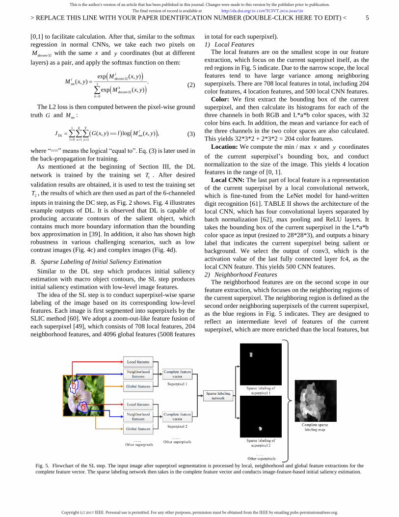
B. Sparse Labeling of Initial Saliency Estimation
Similar to the DL step which produces initial saliency
estimation with macro object contours, the SL step produces
initial saliency estimation with low-level image features.
The idea of the SL step is to conduct superpixel-wise sparse
labeling of the image based on its corresponding low-level
features. Each image is first segmented into superpixels by the
SLIC method [60]. We adopt a zoom-out-like feature fusion of
each superpixel [49], which consists of 708 local features, 204
neighborhood features, and 4096 global features (5008 features
in total for each superpixel).
1) Local Features
The local features are on the smallest scope in our feature
extraction, which focus on the current superpixel itself, as the
red regions in Fig. 5 indicate. Due to the narrow scope, the local
features tend to have large variance among neighboring
superpixels. There are 708 local features in total, including 204
color features, 4 location features, and 500 local CNN features.
Color: We first extract the bounding box of the current
superpixel, and then calculate its histograms for each of the
three channels in both RGB and L*a*b color spaces, with 32
color bins each. In addition, the mean and variance for each of
the three channels in the two color spaces are also calculated.
This yields 32*3*2 + 2*3*2 = 204 color features.
Location: We compute the min / max x and y coordinates
of the current superpixel’s bounding box, and conduct
normalization to the size of the image. This yields 4 location
features in the range of [0, 1].
Local CNN: The last part of local feature is a representation
of the current superpixel by a local convolutional network,
which is fine-tuned from the LeNet model for hand-written
digit recognition [61]. TABLE II shows the architecture of the
local CNN, which has four convolutional layers separated by
batch normalization [62], max pooling and ReLU layers. It
takes the bounding box of the current superpixel in the L*a*b
color space as input (resized to 28*28*3), and outputs a binary
label that indicates the current superpixel being salient or
background. We select the output of conv3, which is the
activation value of the last fully connected layer fc4, as the
local CNN feature. This yields 500 CNN features.
2) Neighborhood Features
The neighborhood features are on the second scope in our
feature extraction, which focuses on the neighboring regions of
the current superpixel. The neighboring region is defined as the
second order neighboring superpixels of the current superpixel,
as the blue regions in Fig. 5 indicates. They are designed to
reflect an intermediate level of features of the current
superpixel, which are more enriched than the local features, but
Fig. 5. Flowchart of the SL step. The input image after superpixel segmentation is processed by local, neighborhood and global feature extractions for the
complete feature vector. The sparse labeling network then takes in the complete feature vector and conducts image-feature-based initial saliency estimation.
This is the author's version of an article that has been published in this journal. Changes were made to this version by the publisher prior to publication.The final version of record is available at http://dx.doi.org/10.1109/TCSVT.2016.2646720
Copyright (c) 2017 IEEE. Personal use is permitted. For any other purposes, permission must be obtained from the IEEE by emailing [email protected].

> REPLACE THIS LINE WITH YOUR PAPER IDENTIFICATION NUMBER (DOUBLE-CLICK HERE TO EDIT) <
6
are less macro-scoped than the global features. Due to its
definition, the neighborhood features are expected to have
lower variance among different superpixels than the local
features. We adopt the same set of color features defined in the
previous section as the neighborhood features, which yields
204 features.
3) Global Features
The global features consist of representations of the whole
image, as the yellow region (outer boundary) in Fig. 5 indicates.
We use a CNN designed for ImageNet classification to generate
the global features. By considering the overall performance, the
VGG-16 model [58] is adopted, which is the same model used
in the DC step (see Section IV.B for detailed discussion).
Images are resized to 224*224 before being fed into the
network, and the 1*1*4096 activation value of the last fully
connected layer is taken as the global feature. Following [49],
we directly use the pre-trained network without fine-tuning.
4) SL Network Training
By performing the feature extraction steps above, a 1*5008
feature vector will be generated per superpixel per image. We
then establish the SL network with three fully connected layers
(see Section IV.B for detailed discussion), which takes the
feature vectors as inputs, and output a binary label indicating
the saliency of the current superpixel. After training for enough
epochs, the SL network is used to generate the low-level feature
based initial saliency channel for the next DC step.
C. Sparse Labeling of Final Saliency Map
While the DL and SL steps are designed to provide coarse
initial saliency estimations, the DC step is designed to generate
the final saliency map with superpixel-wise binary sparse
labeling, i.e. obtain the saliency of each individual superpixel in
the image via DNN-based classification, and then integrate
them together to form the complete final saliency map, as
shown in Fig. 2. Considering the overall performance, we adopt
the VGG-16 [58] as the baseline model of our DC network (see
Section IV.B for detailed discussion). TABLE III shows the
architecture of the DC network. The input structure of DC,
being one of our key novelties, is 6-channeled data with fixed
size as 224*224*6. The first three channels are the RGB data
from the image; the fourth and fifth channels are the initial
saliency estimations from the DL and SL steps, respectively
(both resized to 224*224); and the sixth channel is the
superpixel indication channel, which precisely marks the
current to-be-classified superpixel, as the “Superpixel
indication channel” in Fig. 2 indicates.
To obtain the superpixel indication channel, we first segment
the image into superpixels, also by the SLIC method used in
Section III.B. The to-be-classified superpixel is then selected
and marked on a 224*224 black background, i.e. assigning the
pixels within the superpixel as maximum intensity, while all the
other pixels remain zero. Note that the superpxiel indication
channel is the only channel to differentiate the inputs of
different superpixels from the same image. Hence, provided
that the number of images and number of superpixels per image
are assigned by imN and spN , respectively, there will be
im spN N samples in total.
Let iY be the activation value of the fc8 layer for the i-th
superpixel, whose size is changed from the originally 1000 to 2,
indicating binary classification (salient or background). A
softmax loss layer is applied afterwards to compute the
logarithm loss, with spN as the batch size:
1
1log (1 )log(1 ) ,
spN
T
DC i i i i C j j
i jsp
J G P G P W WN
(4)
where
exp (1)
exp (0) exp (1)
i
i
i i
YP
Y Y
(5)
is the softmax probability of i being salient; [0,1]iG is the
ground truth label of i ; C is the weight decay parameter; j
stands for the layers with trainable weights of the DC network;
and jW is the weight vector of layer j .
We then train DC by the 2T dataset, as mentioned at the start
of Section III, with spN samples per batch and imN
batches in
total. As for testing, the probability iP in (5) is adopted as the
saliency value for the superpixel i, which is assigned to all the
pixels within i. And the final saliency map is formed when all
TABLE II ARCHITECTURE OF OUR LOCAL CNN
Layer Type Output Size Conv (size,
channel, pad) Max Pooling
input in 28*28*3 N/A N/A
conv1 c+b+p 12*12*20 5*5,20,0 2*2
conv2 c+b+p 4*4*50 5*5,50,0 2*2
conv3 c+b+r 1*1*500 4*4,500,0 N/A
fc4 fc+r 1*1*2 1*1,2,0 N/A
loss sm+log 1*1 N/A N/A
Annotations - in: input layer; c: convolutional layer; b: batch normalization
layer; p: pooling layer; r: ReLU layer; fc: fully connected layer; sm: softmax
layer; log: log loss layer.
TABLE III ARCHITECTURE OF OUR DC NETWORK
Layer Type Output Size Conv (size,
channel, pad) Max Pooling
input in 224*224*6 N/A N/A
conv1_1 c+b+r 224*224*64 3*3,64,1 N/A
conv1_2 c+b+r 112*112*64 3*3,64,1 2*2
conv2_1 c+b+r 112*112*128 3*3,128,1 N/A
conv2_2 c+b+r 56*56*128 3*3,128,1 2*2
conv3_1 c+b+r 56*56*256 3*3,256,1 N/A
conv3_2 c+b+r 56*56*256 3*3,256,1 N/A
conv3_3 c+b+r 28*28*256 3*3,256,1 2*2
conv4_1 c+b+r 28*28*512 3*3,512,1 2*2
conv4_2 c+b+r 28*28*512 3*3,512,1 N/A
conv4_3 c+b+r 14*14*512 3*3,512,1 2*2
conv5_1 c+b+r 14*14*512 3*3,512,1 N/A
conv5_2 c+b+r 14*14*512 3*3,512,1 N/A
conv5_3 c+b+r 7*7*512 3*3,512,1 2*2
fc6 fc+r 1*1*4096 7*7,4096,0 N/A
fc7 fc+r 1*1*4096 1*1,4096,0 N/A
fc8 fc+r 1*1*2 1*1,2,0 N/A
loss sm+log 1*1 N/A N/A
Annotations - in: input layer; c: convolutional layer; b: batch normalization layer; p: pooling layer; r: ReLU layer; fc: fully connected layer; sm: softmax
layer; log: log loss layer.
This is the author's version of an article that has been published in this journal. Changes were made to this version by the publisher prior to publication.The final version of record is available at http://dx.doi.org/10.1109/TCSVT.2016.2646720
Copyright (c) 2017 IEEE. Personal use is permitted. For any other purposes, permission must be obtained from the IEEE by emailing [email protected].

> REPLACE THIS LINE WITH YOUR PAPER IDENTIFICATION NUMBER (DOUBLE-CLICK HERE TO EDIT) <
7
of the superpixels in the current image have obtained their
corresponding saliency values, as indicated in Fig. 2.
The major advantage of DC is attributed to its 6-channeled
input structure. Unlike existing DNN-based methods like [2],
[38] that only use RGB or other features from the current image
itself, DC integrates two coarse guiding channels via dense
labeling (DL) and sparse labeling (SL). The two guiding
channels provide reliable prior knowledge with learned
high-level features from the entire training dataset, and can
accurately approximate the salient region as well as exclude
false salient proposals. The 6-channeled input structure also
contains the superpixel indication channel, which directly and
precisely marks the current to-be-classified superpixel, unlike
[2] which only vaguely indicates the superpixel by putting it to
the image center. The examples in Fig. 6 exhibit the combined
strength of the DL, SL and DC steps. Note that DL and SL
contribute complementarily to the DC step (i.e. the final output
of DSL), especially in cases where one of DL or SL encounters
difficulty in estimating the initial saliency accurately, as seen in
Fig. 6c and Fig. 6d. The combination of DL and SL thus
significantly increases the overall robustness of DSL.
IV. EXPERIMENTS
A. Experiment Setup
1) Datasets
Since DL and SL are both serially connected to DC (Fig. 2),
it is necessary to use two independent training sets for DL / SL
and DC respectively, in order to conduct fair trainings.
For the training of DL and SL, we use the DUT-OMRON
dataset [1], which contains 5,168 manually selected high
quality images and corresponding pixel-wise ground truth. We
randomly select 80% of the images for training, and the rest 20%
images for validation.
For the training of DC, we use the MSRA10K dataset [17],
which contains 10,000 randomly chosen images from the
MSRA dataset [13], and their corresponding pixel-wise ground
truth. To make the comparison with state-of-the-art methods
fair, we follow [2] and randomly choose 80% of the images for
training, and the rest 20% images for validation.
For testing, we adopt six well-recognized public datasets,
namely ECSSD [30], PASCAL-S [63], SED1 [64], SED2 [64],
THUR15K [65], and HKU-IS [59]. The ECSSD dataset
contains 1,000 complex images with diversified contexts. The
PASCAL-S dataset is a subset of the PASCAL-S VOC
segmentation challenge [66], which contains 850 images with
highly challenging backgrounds. The SED1 and SED2 are two
datasets designed for saliency detection, with 100 images each;
the images of SED1 contain one salient object, while the
images of SED2 contain two salient objects. The THUR15K
dataset contains 15,000 images, among which we only use the
6,233 images with pixel-wise ground truth. For the HKU-IS
dataset, we only use the 1,447 images in the test set that have no
overlap with any of our comparison methods’ training set in our
following experiments.
2) Evaluation Metrics
Following a recent saliency detection benchmark [67], we
choose the precision-recall (PR) curve, F-measure, and mean
absolute error (MAE) as our evaluation metrics.
The precision and recall values are obtained by binarizing the
saliency map with integer thresholds between 0 and 255. The
precision value equals to the ratio of retrieved salient pixels to
all the pixels retrieved, while the recall value equals to the ratio
of retrieved salient pixels to all salient pixels in the image. The
PR curve is plotted by the precision and recall values at each
threshold point.
The F-measure is a weighted average between precision and
recall, which is calculated as:
2
2
(1 ),
precision recallF
precision recall
(6)
where 2 is set to 0.3 based on most existing methods. As
suggested in [68], the average F-measure of a PR curve equals
to its maximum single-point F-measure.
The MAE is the mean of the absolute difference between the
saliency map S and the pixel-wise ground truth G :
1
1( ) ( ) .
N
i
MAE S i G iN
(7)
Different to precision, recall and F-measure, smaller MAE
means higher performance.
3) Implementation
Our method is implemented on MatConvNet [69], which is a
MATLAB toolbox of CNN with various extensibilities. The
machine used for our experiments is a PC with Intel 6-Core
i7-5820K 3.3GHz CPU, 64GB RAM, GeForce GTX TITAN X
12GB GPU, and 64-bit Ubuntu 14.04.3 LTS. Software
dependencies include CUDA 7.0 and cuDNN v3. All images
are stored on SSD, which accelerates reading speed. The source
code of our proposed DSL method is available online:
https://github.com/yuanyc06/dsl.
B. Design Option Analyses
1) Parameter of the DL Step
The DL network is trained on the DUT-OMRON dataset for
50 epochs, with 50-point logarithm space between 10-3
and 10-4
as the learning rate. As described in Section III.A, the images
Fig. 6. Example outputs of the DL, SL, and DC steps. Note that DL and SL
contributes complementarily to the DC step, which generates the final output
of the proposed DSL method.
This is the author's version of an article that has been published in this journal. Changes were made to this version by the publisher prior to publication.The final version of record is available at http://dx.doi.org/10.1109/TCSVT.2016.2646720
Copyright (c) 2017 IEEE. Personal use is permitted. For any other purposes, permission must be obtained from the IEEE by emailing [email protected].
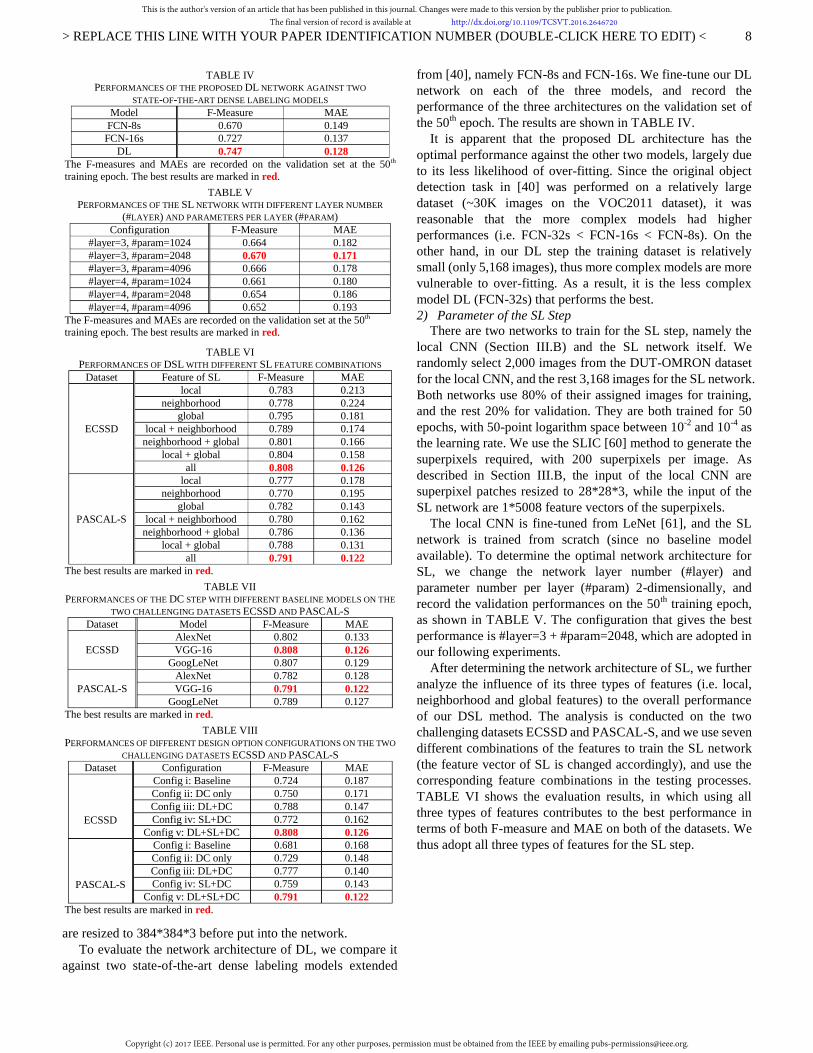
> REPLACE THIS LINE WITH YOUR PAPER IDENTIFICATION NUMBER (DOUBLE-CLICK HERE TO EDIT) <
8
are resized to 384*384*3 before put into the network.
To evaluate the network architecture of DL, we compare it
against two state-of-the-art dense labeling models extended
from [40], namely FCN-8s and FCN-16s. We fine-tune our DL
network on each of the three models, and record the
performance of the three architectures on the validation set of
the 50th
epoch. The results are shown in TABLE IV.
It is apparent that the proposed DL architecture has the
optimal performance against the other two models, largely due
to its less likelihood of over-fitting. Since the original object
detection task in [40] was performed on a relatively large
dataset (~30K images on the VOC2011 dataset), it was
reasonable that the more complex models had higher
performances (i.e. FCN-32s < FCN-16s < FCN-8s). On the
other hand, in our DL step the training dataset is relatively
small (only 5,168 images), thus more complex models are more
vulnerable to over-fitting. As a result, it is the less complex
model DL (FCN-32s) that performs the best.
2) Parameter of the SL Step
There are two networks to train for the SL step, namely the
local CNN (Section III.B) and the SL network itself. We
randomly select 2,000 images from the DUT-OMRON dataset
for the local CNN, and the rest 3,168 images for the SL network.
Both networks use 80% of their assigned images for training,
and the rest 20% for validation. They are both trained for 50
epochs, with 50-point logarithm space between 10-2
and 10-4
as
the learning rate. We use the SLIC [60] method to generate the
superpixels required, with 200 superpixels per image. As
described in Section III.B, the input of the local CNN are
superpixel patches resized to 28*28*3, while the input of the
SL network are 1*5008 feature vectors of the superpixels.
The local CNN is fine-tuned from LeNet [61], and the SL
network is trained from scratch (since no baseline model
available). To determine the optimal network architecture for
SL, we change the network layer number (#layer) and
parameter number per layer (#param) 2-dimensionally, and
record the validation performances on the 50th
training epoch,
as shown in TABLE V. The configuration that gives the best
performance is #layer=3 + #param=2048, which are adopted in
our following experiments.
After determining the network architecture of SL, we further
analyze the influence of its three types of features (i.e. local,
neighborhood and global features) to the overall performance
of our DSL method. The analysis is conducted on the two
challenging datasets ECSSD and PASCAL-S, and we use seven
different combinations of the features to train the SL network
(the feature vector of SL is changed accordingly), and use the
corresponding feature combinations in the testing processes.
TABLE VI shows the evaluation results, in which using all
three types of features contributes to the best performance in
terms of both F-measure and MAE on both of the datasets. We
thus adopt all three types of features for the SL step.
TABLE IV PERFORMANCES OF THE PROPOSED DL NETWORK AGAINST TWO
STATE-OF-THE-ART DENSE LABELING MODELS
Model F-Measure MAE
FCN-8s 0.670 0.149
FCN-16s 0.727 0.137
DL 0.747 0.128
The F-measures and MAEs are recorded on the validation set at the 50th
training epoch. The best results are marked in red.
TABLE V PERFORMANCES OF THE SL NETWORK WITH DIFFERENT LAYER NUMBER
(#LAYER) AND PARAMETERS PER LAYER (#PARAM)
Configuration F-Measure MAE
#layer=3, #param=1024 0.664 0.182
#layer=3, #param=2048 0.670 0.171
#layer=3, #param=4096 0.666 0.178
#layer=4, #param=1024 0.661 0.180
#layer=4, #param=2048 0.654 0.186
#layer=4, #param=4096 0.652 0.193
The F-measures and MAEs are recorded on the validation set at the 50th training epoch. The best results are marked in red.
TABLE VI PERFORMANCES OF DSL WITH DIFFERENT SL FEATURE COMBINATIONS
Dataset Feature of SL F-Measure MAE
ECSSD
local 0.783 0.213
neighborhood 0.778 0.224
global 0.795 0.181
local + neighborhood 0.789 0.174
neighborhood + global 0.801 0.166
local + global 0.804 0.158
all 0.808 0.126
PASCAL-S
local 0.777 0.178
neighborhood 0.770 0.195
global 0.782 0.143
local + neighborhood 0.780 0.162
neighborhood + global 0.786 0.136
local + global 0.788 0.131
all 0.791 0.122
The best results are marked in red.
TABLE VII PERFORMANCES OF THE DC STEP WITH DIFFERENT BASELINE MODELS ON THE
TWO CHALLENGING DATASETS ECSSD AND PASCAL-S
Dataset Model F-Measure MAE
ECSSD
AlexNet 0.802 0.133
VGG-16 0.808 0.126
GoogLeNet 0.807 0.129
PASCAL-S
AlexNet 0.782 0.128
VGG-16 0.791 0.122
GoogLeNet 0.789 0.127
The best results are marked in red.
TABLE VIII PERFORMANCES OF DIFFERENT DESIGN OPTION CONFIGURATIONS ON THE TWO
CHALLENGING DATASETS ECSSD AND PASCAL-S
Dataset Configuration F-Measure MAE
ECSSD
Config i: Baseline 0.724 0.187
Config ii: DC only 0.750 0.171
Config iii: DL+DC 0.788 0.147
Config iv: SL+DC 0.772 0.162
Config v: DL+SL+DC 0.808 0.126
PASCAL-S
Config i: Baseline 0.681 0.168
Config ii: DC only 0.729 0.148
Config iii: DL+DC 0.777 0.140
Config iv: SL+DC 0.759 0.143
Config v: DL+SL+DC 0.791 0.122
The best results are marked in red.
This is the author's version of an article that has been published in this journal. Changes were made to this version by the publisher prior to publication.The final version of record is available at http://dx.doi.org/10.1109/TCSVT.2016.2646720
Copyright (c) 2017 IEEE. Personal use is permitted. For any other purposes, permission must be obtained from the IEEE by emailing [email protected].

> REPLACE THIS LINE WITH YOUR PAPER IDENTIFICATION NUMBER (DOUBLE-CLICK HERE TO EDIT) <
9
3) Parameter of the DC Step
The DC network is trained on the MSRA10K dataset. We
first feedforward MSRA10K through DL and SL to obtain the
two initial saliency channels of its images, and then form the
6-channeled inputs for DC. The DC network is trained for 20
epochs, with 20-point logarithm space between 10-2
and 10-4
as
the learning rate. The superpixels are generated by the SLIC
method as well, with 200 superpixels per image.
To determine the best baseline model, we fine-tune the DC
network on three state-of-the-art image classification models,
namely AlexNet [47], VGG-16 [58], and GoogLeNet [5]. We
record their performances on the two challenging datasets
ECSSD and PASCAL-S in TABLE VII. It is observed that
VGG-16 has the best overall performance than the other two
models, and previous works have proved its steadiness and
robustness in various computer vision tasks [40], [70-72]. We
thus adopt VGG-16 as our baseline model for the DC step.
4) Contribution Comparison
Next, we examine the contributions of the three steps (i.e.
DL, SL and DC) in improving the performance of our method.
We take the “pad-and-center” method in [2] as the comparison
baseline, and compare five different configurations below:
i. Baseline: the local pad-and-center model in [2]; the
network takes padded image as input (224*224*3) (without the
superpixel indication channel);
ii. DC only: the input of DC is thus 224*224*4 (with the
superpixel indication channel, but without the DL and SL
channels);
iii. DL and DC: the input of DC is thus 224*224*5 (with the
superpixel indication channel, but without the SL channel);
iv. SL and DC: the input of DC is thus 224*224*5 (with the
superpixel indication channel, but without the DL channel);
v. Complete DSL model: the DC network takes the
224*224*6 input with all of the 6 channels.
Similarly to the previous section, we record the
performances of the five configurations above on the two
challenging datasets ECSSD and PASCAL-S. The results are
listed in TABLE VIII. We see that the complete DSL
framework (Configuration v: DL+SL+DC) notably
outperforms the other four configurations, which indicates that
DL, SL and DC all have significant contributions in improving
the overall performance of DSL.
C. Comparison with Conventional Methods
Next, we compare our proposed DSL method with ten
state-of-the-art conventional (non-learning based) saliency
detection methods, namely SF [10], GR [73], MC [19], MR [1],
DSR [20], HS [30], RBD [25], RR [42], BSCA [23], and BL
[45]. All of the ten methods are published after 2012, and the
last three methods are recently published in 2015. As
mentioned in Section IV.A, the experiments are conducted on
the six datasets ECSSD, PASCAL-S, SED1, SED2, THUR15K
and HKU-IS. The results are shown in Fig. 7 and TABLE IX.
We first notice that DSL not only achieves the best
performance on all of the dataset in terms of both F-measure
and MAE, but also exceeds the comparison methods with
dominant advantages. We first analyze the two challenging
datasets ECSSD and PASCAL-S, where DSL’s PR curves are
greatly higher than the comparison methods, and its F-measures
and MAEs have shown significantly large gaps against the
second best methods. To be more specific, its F-measures are
12.5% and 18.2% higher than the second best (0.808 to 0.718,
and 0.791 to 0.669), and its MAEs are 78.6% and 65.6% lower
than the second best (0.126 to 0.225, and 0.122 to 0.202). We
attribute the greatly improved performance of DSL to its
integrated structure of multiple DNNs, in which both dense and
sparse labeling show their strength in extracting the high-level
features of the image, as well as their combined advantage that
further boost the saliency classification accuracy.
(a) (b) (c)
(d) (e) (f) Fig. 7. PR curves of DSL against ten state-of-the-art conventional saliency detection methods. (a) ECSSD; (b) PASCAL-S; (c) SED1; (d) SED2; (e) THUR15K; (f) HKU-IS.
This is the author's version of an article that has been published in this journal. Changes were made to this version by the publisher prior to publication.The final version of record is available at http://dx.doi.org/10.1109/TCSVT.2016.2646720
Copyright (c) 2017 IEEE. Personal use is permitted. For any other purposes, permission must be obtained from the IEEE by emailing [email protected].

> REPLACE THIS LINE WITH YOUR PAPER IDENTIFICATION NUMBER (DOUBLE-CLICK HERE TO EDIT) <
10
TABLE IX
QUANTITATIVE EVALUATION RESULTS OF DSL AGAINST TEN STATE-OF-THE-ART CONVENTIONAL SALIENCY DETECTION METHODS
Dataset Metric SF GR MC MR DSR HS RBD RR BSCA BL DSL
ECSSD F-Measure 0.549 0.642 0.703 0.708 0.699 0.698 0.686 0.710 0.718 0.716 0.808
MAE 0.268 0.317 0.251 0.236 0.226 0.269 0.225 0.234 0.233 0.262 0.126
PASCAL-S F-Measure 0.496 0.604 0.668 0.612 0.651 0.645 0.659 0.639 0.669 0.663 0.791
MAE 0.241 0.301 0.232 0.259 0.208 0.264 0.202 0.232 0.224 0.249 0.122
SED1 F-Measure 0.665 0.791 0.844 0.841 0.819 0.825 0.829 0.843 0.832 0.840 0.901
MAE 0.234 0.224 0.164 0.143 0.160 0.163 0.144 0.141 0.155 0.190 0.099
SED2 F-Measure 0.783 0.785 0.775 0.771 0.793 0.791 0.826 0.769 0.780 0.787 0.858
MAE 0.171 0.192 0.180 0.164 0.140 0.195 0.130 0.161 0.158 0.189 0.108
THUR15K F-Measure 0.469 0.551 0.610 0.573 0.611 0.585 0.596 0.590 0.609 0.606 0.730
MAE 0.193 0.264 0.199 0.209 0.139 0.250 0.163 0.185 0.216 0.261 0.123
HKU-IS F-Measure 0.588 0.672 0.723 0.689 0.735 0.706 0.725 0.711 0.722 0.716 0.858
MAE 0.183 0.266 0.201 0.192 0.133 0.253 0.150 0.175 0.210 0.257 0.125
For each row, the top 3 results are marked in red, blue and green, respectively.
(a) (b) (c)
(d) (e) (f)
Fig. 8. PR curves of DSL against six state-of-the-art learning based saliency detection methods. (a) ECSSD; (b) PASCAL-S; (c) SED1; (d) SED2; (e) THUR15K; (f) HKU-IS.
TABLE X QUANTITATIVE EVALUATION RESULTS OF DSL AGAINST SIX STATE-OF-THE-ART LEARNING BASED SALIENCY DETECTION METHODS
Dataset Metric DRFI HDCT MCDL LEGS MDF DISC DSL
ECSSD F-Measure 0.736 0.698 0.748 0.776 0.772 0.756 0.808
MAE 0.226 0.166 0.175 0.182 0.174 0.208 0.126
PASCAL-S F-Measure 0.694 0.652 0.700 0.762 0.768 0.744 0.791
MAE 0.210 0.157 0.160 0.171 0.144 0.172 0.122
SED1 F-Measure 0.864 0.821 0.858 0.867 0.881 0.876 0.901
MAE 0.149 0.183 0.087 0.185 0.158 0.118 0.099
SED2 F-Measure 0.823 0.792 0.785 0.802 0.844 0.780 0.858
MAE 0.140 0.134 0.137 0.104 0.152 0.153 0.108
THUR15K F-Measure 0.666 0.620 0.673 0.688 0.701 0.664 0.730
MAE 0.169 0.163 0.192 0.155 0.140 0.084 0.123
HKU-IS F-Measure 0.775 0.747 0.789 0.837 0.860 0.788 0.858
MAE 0.161 0.155 0.181 0.146 0.209 0.180 0.125
For each row, the top 3 results are marked in red, blue and green, respectively.
TABLE XI EFFICIENCY COMPARISON (SECONDS PER IMAGE)
Method DSR RBD LEGS MDF DSL
Time (s) 0.525 0.341 1.75 1.48 0.695
Code MATLAB MATLAB MATLAB MATLAB MATLAB
This is the author's version of an article that has been published in this journal. Changes were made to this version by the publisher prior to publication.The final version of record is available at http://dx.doi.org/10.1109/TCSVT.2016.2646720
Copyright (c) 2017 IEEE. Personal use is permitted. For any other purposes, permission must be obtained from the IEEE by emailing [email protected].

> REPLACE THIS LINE WITH YOUR PAPER IDENTIFICATION NUMBER (DOUBLE-CLICK HERE TO EDIT) <
11
Image
SF
GR
MC
MR
DSR
HS
RBD
RR
BSCA
BL
DSL
GT
DRFI
MCDL
LEGS
MDF
DISC
(d)(b) (c) (e)(a) (g)(f)
HDCT
Fig. 9. Example saliency maps of different methods. (a) – (c): images with low contrast objects; (d) – (f): image with complex foreground / background patterns; (g): image with highly interfering background.
This is the author's version of an article that has been published in this journal. Changes were made to this version by the publisher prior to publication.The final version of record is available at http://dx.doi.org/10.1109/TCSVT.2016.2646720
Copyright (c) 2017 IEEE. Personal use is permitted. For any other purposes, permission must be obtained from the IEEE by emailing [email protected].

> REPLACE THIS LINE WITH YOUR PAPER IDENTIFICATION NUMBER (DOUBLE-CLICK HERE TO EDIT) <
12
DSL behaves similarly on the other four datasets, where it
shows dominant advantages on both PR curves and evaluation
metrics against all of the comparison methods. What is
mentionable is that the advantage of DSL on SED2 is relatively
small compared to its advantages on the other datasets. This is
mainly due to the single-object training set we used, while all of
the images in SED2 contain two salient objects.
D. Comparison with Learning Based Methods
Since DSL is learning based, it is not surprising that it has
large performance improvements against the conventional
saliency detection methods in Section IV.C. To further evaluate
the effectiveness of DSL, we compare it against six
state-of-the-art learning based methods, namely DRFI [18],
HDCT [74], MCDL [2], LEGS [38], MDF [59] and DISC [70].
All of the six methods are published after 2013, and the last
four methods are recently published in 2015. The experiments
are conducted on the same six datasets in Section IV.C, and the
comparison results are shown in TABLE X.
It is observed that the overall performances of the learning
based methods are significantly higher than those of the
conventional methods in TABLE IX, due to the high-level
features involved in their learning processes. Nevertheless,
DSL still maintains significant advantages against the
comparison learning based methods. It achieves optimal
performance on five out of six F-measures, and three out of six
MAEs, and achieves the second place on all of the other
evaluations with close distance to the optimal. We note that
MDF is the only method that uses the training set of HKU-IS
(3,000 images) in its training process, so it is expected to have
high performance on the test set of HKU-IS; nevertheless, DSL
behaves closely against MDF in F-measure, and even achieves
better MAE with significant advantage. We attribute the high
performance of DSL to its combination of dense and sparse
labeling that exploits both macro object contours and the local
low-level image features. DSL’s superior performance against
the state-of-the-art learning based methods further validates its
effectiveness and robustness in various cases.
To demonstrate the greatly improved performance of DSL
more straightforwardly, we select typical saliency map
examples of both conventional methods and learning based
methods, which are assembled together in Fig. 9. We note that
DSL exhibits high accuracy and robustness on various
challenging scenarios, including images with low contrast
objects (Fig. 9a - Fig. 9c), images with complex foreground /
background patterns (Fig. 9d - Fig. 9f), and image with highly
interfering background (Fig. 9g).
E. Efficiency
To evaluate the efficiency of DSL, we select two comparison
methods from both the conventional methods and the learning
based methods that have the highest performances among
TABLE IX and TABLE X, namely DSR, RBD, LEGS and
MDF. We record their average running time per image on the
same machine described in Section IV.A.3), and the results are
shown in TABLE XI. Since all of the five methods are
implemented in MATLAB, the efficiency comparison is fair for
coding language. It is observed that besides its premium
performances against the comparison methods, DSL also
achieves comparable running time to the conventional methods,
and notably faster speed than the learning based methods. The
three steps of DL, SL and DC take approximately 5%, 60% and
35% of the total running time, respectively.
F. Limitation
As mentioned in Section IV.C, currently DSL’s high
performance is only guaranteed on single-object images, which
is mainly due to the single-object training set we used for the
DL, SL and DC networks. This issue, however, is an inherent
limitation with all learning based methods that depend on the
training data. We can solve this issue by extending our training
set with broader categories of images, which will be covered in
our future works.
V. CONCLUSION
In this paper, we propose a novel DNN-based saliency
detection method, DSL, which conducts dense and sparse
labeling of image saliency with multi-dimensional features.
DSL consists of three major steps, namely DL, SL and DC. The
DL and SL steps conduct effective initial saliency estimations
with both macro object contours and local low-level features,
while the final DC network establishes a 6-channeled data
structure as input, and conducts accurate final saliency
classification. Our DSL method achieves remarkably higher
performance against sixteen state-of-the-art saliency detection
methods (including ten conventional methods and six learning
based methods) on six well-recognized public datasets, in terms
of both accuracy and robustness. As future research, we will
explore adaptations of our method to other application areas,
such as medical image segmentation and video data processing.
REFERENCES
[1] C. Yang, L. Zhang, H. Lu, X. Ruan, and M.-H. Yang, "Saliency detection
via graph-based manifold ranking," in Proc. IEEE Conf. Comput. Vision Pattern Recognition (CVPR), Portland, OR, USA, Jun. 2013, pp.
3166-3173.
[2] R. Zhao, W. Ouyang, H. Li, and X. Wang, "Saliency detection by multi-context deep learning," in Proc. IEEE Conf. Comput. Vision Pattern
Recognition (CVPR), Boston, MA, USA, Jun. 2015, pp. 1265-1274.
[3] L. Itti, C. Koch, and E. Niebur, "A model of saliency-based visual
attention for rapid scene analysis," IEEE Trans. Pattern Anal. Mach.
Intell., vol. 20, no. 11, pp. 1254-1259, Nov. 1998.
[4] C. Rother, V. Kolmogorov, and A. Blake, "Grabcut: Interactive foreground extraction using iterated graph cuts," ACM Trans. Graph., vol.
23, no. 3, pp. 309-314, Sep. 2004.
[5] C. Szegedy, W. Liu, Y. Jia, P. Sermanet, S. Reed, D. Anguelov, et al., "Going deeper with convolutions," arXiv preprint arXiv:1409.4842,
2014.
[6] U. Rutishauser, D. Walther, C. Koch, and P. Perona, "Is bottom-up attention useful for object recognition?," in Proc. IEEE Conf. Comput.
Vision Pattern Recognition (CVPR), Washington, D.C., USA, Jun. 2004,
pp. II-37-II-44 Vol. 2. [7] V. Mahadevan and N. Vasconcelos, "Saliency-based discriminant
tracking," in Proc. IEEE Conf. Comput. Vision Pattern Recognition
(CVPR), Miami, FL, USA, Jun. 2009, pp. 1007-1013. [8] J. Wang, L. Quan, J. Sun, X. Tang, and H.-Y. Shum, "Picture collage," in
Proc. IEEE Conf. Comput. Vision Pattern Recognition (CVPR), New
York City, NY, USA, Jun. 2006, pp. 347-354.
This is the author's version of an article that has been published in this journal. Changes were made to this version by the publisher prior to publication.The final version of record is available at http://dx.doi.org/10.1109/TCSVT.2016.2646720
Copyright (c) 2017 IEEE. Personal use is permitted. For any other purposes, permission must be obtained from the IEEE by emailing [email protected].
> REPLACE THIS LINE WITH YOUR PAPER IDENTIFICATION NUMBER (DOUBLE-CLICK HERE TO EDIT) <
13
[9] T. Wang, T. Mei, X.-S. Hua, X.-L. Liu, and H.-Q. Zhou, "Video collage:
A novel presentation of video sequence," in Proc. IEEE Int. Conf. Multimedia Expo (ICME), Beijing, China, Jul. 2007, pp. 1479-1482.
[10] F. Perazzi, P. Krahenbuhl, Y. Pritch, and A. Hornung, "Saliency filters:
Contrast based filtering for salient region detection," in Proc. IEEE Conf. Comput. Vision Pattern Recognition (CVPR), Providence, RI, USA, Jun.
2012, pp. 733-740.
[11] P. Wang, D. Zhang, J. Wang, Z. Wu, X.-S. Hua, and S. Li, "Color filter for image search," in Proc. ACM Int. Conf. Multimedia (ACMMM), Nara,
Japan, Oct. 2012, pp. 1327-1328.
[12] T. Judd, K. Ehinger, F. Durand, and A. Torralba, "Learning to predict where humans look," in Proc. IEEE Int. Conf. Comput. Vision (ICCV),
Kyoto, Japan, Sep. 2009, pp. 2106-2113.
[13] T. Liu, Z. Yuan, J. Sun, J. Wang, N. Zheng, X. Tang, et al., "Learning to detect a salient object," IEEE Trans. Pattern Anal. Mach. Intell., vol. 33,
no. 2, pp. 353-367, 2011.
[14] C. Shen and Q. Zhao, "Learning to predict eye fixations for semantic contents using multi-layer sparse network," Neurocomput., vol. 138, pp.
61-68, 2014.
[15] P. F. Felzenszwalb and D. P. Huttenlocher, "Efficient graph-based image
segmentation," Int. J. Comput. Vis., vol. 59, no. 2, pp. 167-181, 2004.
[16] R. Fergus, P. Perona, and A. Zisserman, "Object class recognition by
unsupervised scale-invariant learning," in Proc. IEEE Conf. Comput. Vision Pattern Recognition (CVPR), Madison, WI, USA, Jun. 2003, pp.
II-264-II-271 vol. 2.
[17] M.-M. Cheng, G.-X. Zhang, N. J. Mitra, X. Huang, and S.-M. Hu, "Global contrast based salient region detection," in Proc. IEEE Conf. Comput.
Vision Pattern Recognition (CVPR), Colorado Springs, CO, USA, Jun. 2011, pp. 409-416.
[18] H. Jiang, J. Wang, Z. Yuan, Y. Wu, N. Zheng, and S. Li, "Salient object
detection: A discriminative regional feature integration approach," in Proc. IEEE Conf. Comput. Vision Pattern Recognition (CVPR), Portland,
OR, USA, Jun. 2013, pp. 2083-2090.
[19] B. Jiang, L. Zhang, H. Lu, C. Yang, and M.-H. Yang, "Saliency detection via absorbing markov chain," in Proc. IEEE Int. Conf. Comput. Vision
(ICCV), Sydney, NSW, Australia, Dec. 2013, pp. 1665-1672.
[20] X. Li, H. Lu, L. Zhang, X. Ruan, and M.-H. Yang, "Saliency detection via
dense and sparse reconstruction," in Proc. IEEE Int. Conf. Comput. Vision
(ICCV), Sydney, NSW, Australia, Dec. 2013, pp. 2976-2983.
[21] R. Achanta, S. Hemami, F. Estrada, and S. Susstrunk, "Frequency-tuned salient region detection," in Proc. IEEE Conf. Comput. Vision Pattern
Recognition (CVPR), Miami, FL, USA, Jun. 2009, pp. 1597-1604.
[22] X. Hou and L. Zhang, "Saliency detection: A spectral residual approach," in Proc. IEEE Conf. Comput. Vision Pattern Recognition (CVPR),
Minneapolis, MN, USA, Jun. 2007, pp. 1-8.
[23] Y. Qin, H. Lu, Y. Xu, and H. Wang, "Saliency detection via cellular automata," in Proc. IEEE Conf. Comput. Vision Pattern Recognition
(CVPR), Boston, MA, USA, Jun. 2015, pp. 110-119.
[24] Y. Wei, F. Wen, W. Zhu, and J. Sun, "Geodesic saliency using background priors," in Comput. Vision–ECCV, ed: Springer, 2012, pp.
29-42.
[25] W. Zhu, S. Liang, Y. Wei, and J. Sun, "Saliency Optimization from Robust Background Detection," in Proc. IEEE Conf. Comput. Vision
Pattern Recognition (CVPR), Columbus, OH, USA, Jun. 2014, pp.
2814-2821. [26] K.-Y. Chang, T.-L. Liu, H.-T. Chen, and S.-H. Lai, "Fusing generic
objectness and visual saliency for salient object detection," in Proc. IEEE
Conf. Comput. Vision Pattern Recognition (CVPR), Colorado Springs, CO, USA, Jun. 2011, pp. 914-921.
[27] S. Goferman, L. Zelnik-Manor, and A. Tal, "Context-aware saliency
detection," IEEE Trans. Pattern Anal. Mach. Intell., vol. 34, no. 10, pp. 1915-1926, Oct. 2012.
[28] J. Harel, C. Koch, and P. Perona, "Graph-based visual saliency," in Adv.
Neural Inform. Process. Sys., Dec. 2006, pp. 545-552. [29] E. Rahtu, J. Kannala, M. Salo, and J. Heikkilä, "Segmenting salient
objects from images and videos," in Comput. Vision–ECCV, ed: Springer,
2010, pp. 366-379. [30] Q. Yan, L. Xu, J. Shi, and J. Jia, "Hierarchical saliency detection," in
Proc. IEEE Conf. Comput. Vision Pattern Recognition (CVPR), Portland,
OR, USA, Jun. 2013, pp. 1155-1162. [31] L. Zhang, M. H. Tong, T. K. Marks, H. Shan, and G. W. Cottrell, "SUN: A
Bayesian framework for saliency using natural statistics," J. Vis., vol. 8,
no. 7, p. 32, 2008.
[32] J. Yang and M.-H. Yang, "Top-down visual saliency via joint crf and
dictionary learning," in Proc. IEEE Conf. Comput. Vision Pattern Recognition (CVPR), Providence, RI, USA, Jun. 2012, pp. 2296-2303.
[33] D. A. Klein and S. Frintrop, "Center-surround divergence of feature
statistics for salient object detection," in Proc. IEEE Int. Conf. Comput. Vision (ICCV), Barcelona, Spain, Nov. 2011, pp. 2214-2219.
[34] K. Fu, C. Gong, J. Yang, Y. Zhou, and I. Yu-Hua Gu, "Superpixel based
color contrast and color distribution driven salient object detection," Signal Process. Image Commun., vol. 28, no. 10, pp. 1448-1463, Jul.
2013.
[35] Y. LeCun, B. Boser, J. S. Denker, D. Henderson, R. E. Howard, W. Hubbard, et al., "Backpropagation applied to handwritten zip code
recognition," Neural Computation, vol. 1, no. 4, pp. 541-551, 1989.
[36] G. E. Hinton and R. R. Salakhutdinov, "Reducing the dimensionality of data with neural networks," Sci., vol. 313, no. 5786, pp. 504-507, 2006.
[37] R. Girshick, J. Donahue, T. Darrell, and J. Malik, "Rich feature
hierarchies for accurate object detection and semantic segmentation," in Proc. IEEE Conf. Comput. Vision Pattern Recognition (CVPR),
Columbus, OH, USA, Jun. 2014, pp. 580-587.
[38] L. Wang, H. Lu, X. Ruan, and M.-H. Yang, "Deep networks for saliency
detection via local estimation and global search," in Proc. IEEE Conf.
Comput. Vision Pattern Recognition (CVPR), Boston, MA, USA, Jun.
2015, pp. 3183-3192. [39] C. Szegedy, A. Toshev, and D. Erhan, "Deep neural networks for object
detection," in Adv. Neural Inform. Process. Sys.2013, pp. 2553-2561.
[40] J. Long, E. Shelhamer, and T. Darrell, "Fully convolutional networks for semantic segmentation," arXiv preprint arXiv:1411.4038, 2014.
[41] J. Sun, H. Lu, and X. Liu, "Saliency Region Detection Based on Markov Absorption Probabilities," IEEE Trans. Image Process., vol. 24, no. 5, pp.
1639-1649, 2015.
[42] C. Li, Y. Yuan, W. Cai, Y. Xia, and D. D. Feng, "Robust saliency detection via regularized random walks ranking," in Proc. IEEE Conf.
Comput. Vision Pattern Recognition (CVPR), Boston, MA, USA, Jun.
2015, pp. 2710-2717. [43] S. Lu, V. Mahadevan, and N. Vasconcelos, "Learning Optimal Seeds for
Diffusion-based Salient Object Detection," in Proc. IEEE Conf. Comput.
Vision Pattern Recognition (CVPR), Portland, OR, USA, Jun. 2013, pp.
2790-2797.
[44] L. Mai, Y. Niu, and F. Liu, "Saliency aggregation: A data-driven
approach," in Proc. IEEE Conf. Comput. Vision Pattern Recognition (CVPR), Portland, OR, USA, Jun. 2013, pp. 1131-1138.
[45] N. Tong, H. Lu, X. Ruan, and M.-H. Yang, "Salient object detection via
bootstrap learning," in Proc. IEEE Conf. Comput. Vision Pattern Recognition (CVPR), Boston, MA, USA, Jun. 2015, pp. 1884-1892.
[46] L. Deng and D. Yu, "Deep learning: methods and applications," Found.
Trends Signal Process., vol. 7, no. 3–4, pp. 197-387, 2014. [47] A. Krizhevsky, I. Sutskever, and G. E. Hinton, "Imagenet classification
with deep convolutional neural networks," in Adv. Neural Inform.
Process. Sys.2012, pp. 1097-1105. [48] P. Sermanet, D. Eigen, X. Zhang, M. Mathieu, R. Fergus, and Y. LeCun,
"Overfeat: Integrated recognition, localization and detection using
convolutional networks," arXiv preprint arXiv:1312.6229, 2013. [49] M. Mostajabi, P. Yadollahpour, and G. Shakhnarovich, "Feedforward
semantic segmentation with zoom-out features," arXiv preprint
arXiv:1412.0774, 2014. [50] L.-C. Chen, G. Papandreou, I. Kokkinos, K. Murphy, and A. L. Yuille,
"Semantic image segmentation with deep convolutional nets and fully
connected crfs," arXiv preprint arXiv:1412.7062, 2014. [51] Y. Sun, X. Wang, and X. Tang, "Deep convolutional network cascade for
facial point detection," in Proc. IEEE Conf. Comput. Vision Pattern
Recognition (CVPR), Portland, OR, USA, Jun. 2013, pp. 3476-3483. [52] Y. Sun, X. Wang, and X. Tang, "Deep learning face representation from
predicting 10,000 classes," in Proc. IEEE Conf. Comput. Vision Pattern
Recognition (CVPR), Columbus, OH, USA, Jun. 2014, pp. 1891-1898. [53] A. Toshev and C. Szegedy, "Deeppose: Human pose estimation via deep
neural networks," in Proc. IEEE Conf. Comput. Vision Pattern
Recognition (CVPR), Columbus, OH, USA, Jun. 2014, pp. 1653-1660. [54] P. Sermanet, K. Kavukcuoglu, S. Chintala, and Y. LeCun, "Pedestrian
detection with unsupervised multi-stage feature learning," in Proc. IEEE
Conf. Comput. Vision Pattern Recognition (CVPR), Portland, OR, USA, Jun. 2013, pp. 3626-3633.
[55] X. Zeng, W. Ouyang, and X. Wang, "Multi-stage contextual deep learning
for pedestrian detection," in Proc. IEEE Int. Conf. Comput. Vision (ICCV), Sydney, NSW, Australia, Dec. 2013, pp. 121-128.
This is the author's version of an article that has been published in this journal. Changes were made to this version by the publisher prior to publication.The final version of record is available at http://dx.doi.org/10.1109/TCSVT.2016.2646720
Copyright (c) 2017 IEEE. Personal use is permitted. For any other purposes, permission must be obtained from the IEEE by emailing [email protected].
> REPLACE THIS LINE WITH YOUR PAPER IDENTIFICATION NUMBER (DOUBLE-CLICK HERE TO EDIT) <
14
[56] P. O. Pinheiro and R. Collobert, "From Image-level to Pixel-level
Labeling with Convolutional Networks," in Proc. IEEE Conf. Comput. Vision Pattern Recognition (CVPR), Boston, MA, USA, Jun. 2015, pp.
1713-1721.
[57] M. D. Zeiler and R. Fergus, "Visualizing and understanding convolutional networks," in Comput. Vision–ECCV, ed: Springer, 2014, pp. 818-833.
[58] K. Simonyan and A. Zisserman, "Very deep convolutional networks for
large-scale image recognition," arXiv preprint arXiv:1409.1556, 2014. [59] G. Li and Y. Yu, "Visual Saliency Based on Multiscale Deep Features,"
arXiv preprint arXiv:1503.08663, 2015.
[60] R. Achanta, A. Shaji, K. Smith, A. Lucchi, P. Fua, and S. Susstrunk, "SLIC superpixels compared to state-of-the-art superpixel methods,"
IEEE Trans. Pattern Anal. Mach. Intell., vol. 34, no. 11, pp. 2274-2282,
Nov. 2012. [61] Y. LeCun, L. Bottou, Y. Bengio, and P. Haffner, "Gradient-based learning
applied to document recognition," Proc. IEEE, vol. 86, no. 11, pp.
2278-2324, 1998. [62] S. Ioffe and C. Szegedy, "Batch normalization: Accelerating deep
network training by reducing internal covariate shift," arXiv preprint
arXiv:1502.03167, 2015.
[63] Y. Li, X. Hou, C. Koch, J. Rehg, and A. Yuille, "The secrets of salient
object segmentation," in Proc. IEEE Conf. Comput. Vision Pattern
Recognition (CVPR), Columbus, OH, USA, Jun. 2014, pp. 4321-4328. [64] S. Alpert, M. Galun, R. Basri, and A. Brandt, "Image segmentation by
probabilistic bottom-up aggregation and cue integration," in Proc. IEEE
Conf. Comput. Vision Pattern Recognition (CVPR), Minneapolis, MN, USA, Jun. 2007, pp. 1-8.
[65] M.-M. Cheng, N. J. Mitra, X. Huang, and S.-M. Hu, "Salientshape: Group saliency in image collections," Visual Comput., vol. 30, no. 4, pp.
443-453, 2014.
[66] M. Everingham, L. Van Gool, C. K. Williams, J. Winn, and A. Zisserman, "The pascal visual object classes (voc) challenge," Int. J. Comput. Vis.,
vol. 88, no. 2, pp. 303-338, Sep. 2010.
[67] A. Borji, D. N. Sihite, and L. Itti, "Salient object detection: A benchmark," in Comput. Vision–ECCV, ed: Springer, 2012, pp. 414-429.
[68] D. R. Martin, C. C. Fowlkes, and J. Malik, "Learning to detect natural
image boundaries using local brightness, color, and texture cues," IEEE Trans. Pattern Anal. Mach. Intell., vol. 26, no. 5, pp. 530-549, May. 2004.
[69] A. Vedaldi and K. Lenc, "MatConvNet-convolutional neural networks for
MATLAB," arXiv preprint arXiv:1412.4564, 2014. [70] T. Chen, L. Lin, L. Liu, X. Luo, and X. Li, "DISC: Deep Image Saliency
Computing via Progressive Representation Learning," arXiv preprint
arXiv:1511.04192, 2015. [71] R. Girshick, "Fast r-cnn," in Proc. IEEE Int. Conf. Comput. Vision
(ICCV), Santiago, Chile, Dec. 2015, pp. 1440-1448.
[72] J. Dai, Y. Li, K. He, and J. Sun, "R-FCN: Object Detection via Region-based Fully Convolutional Networks," arXiv preprint
arXiv:1605.06409, 2016.
[73] C. Yang, L. Zhang, and H. Lu, "Graph-regularized saliency detection with convex-hull-based center prior," IEEE Signal Process. Lett., vol. 20, no.
7, pp. 637-640, 2013.
[74] J. Kim, D. Han, Y.-W. Tai, and J. Kim, "Salient region detection via high-dimensional color transform," in Proc. IEEE Conf. Comput. Vision
Pattern Recognition (CVPR), Columbus, OH, USA, Jun. 2014, pp.
883-890.
Yuchen Yuan received the B. E. degree in biomedical
engineering from Tsinghua University, Beijing, China, in
2010, and the M. S. degree in biomedical engineering from Washington University in St. Louis, St. Louis, MO,
USA, in 2012. He then worked as a senior system
research engineer at Mindray Co., Ltd, Shenzhen, China, from 2012 to 2014.
He is currently a Ph. D. candidate at the School of
Information Technologies, the University of Sydney. His research interests include deep learning, saliency detection, image
segmentation and bioinformatics.
Changyang Li received the Ph.D. degree from the
University of Sydney, Sydney, Australia, in 2012. He is currently a Research Associate with the School of
Information Technologies, the University of Sydney. His
current research interests include image segmentation, pattern recognition, processing for biomedical images,
and multimodality data registration.
Jinman Kim received the B. S. (honours) and Ph. D.
degrees in computer science from the University of
Sydney, Sydney, Australia, in 2001 and 2006, respectively. Since his Ph. D., he has been a research
associate at the leading teaching hospital, the Royal
Prince Alfred. From 2008 to 2012, he was an ARC postdoc research fellow, one year leave (2009-2010) to
join the MIRALab research group, Geneva, Switzerland,
as a Marie Curie senior research fellow. Since 2013, he
has been with the School of IT, the University of Sydney, where he was a senior
lecturer, and became an associate professor in 2016.
His research interests include medical image analysis and visualization, computer aided diagnosis, and Telehealth technologies.
Weidong Cai received the Ph. D. degree in Computer Science from the Basser Department of Computer
Science, The University of Sydney, Sydney, Australia, in
2001. He is currently an Associate Professor in the School of
Information Technologies, Director of the Multimedia
Laboratory in The University of Sydney. He has been a Lead Investigator / Visiting Professor on medical image
analysis and medical computer vision at Surgical
Planning Laboratory (SPL), Harvard Medical School during his 2014 SSP. His
research interests include multimedia computing, medical image analysis,
image / video processing and retrieval, computer vision & pattern recognition,
big data mining, bioimaging informatics, and computational neuroscience.
Dagan Feng received the M. E. degree in Electrical
Engineering & Computer Science (EECS) from Shanghai
Jiao Tong University, Shanghai, China, in 1982, and the M. S. in Biocybernetics and Ph. D. in Computer Science
from the University of California, Los Angeles, CA,
USA, in 1985 and 1988 respectively, where he received the Crump Prize for Excellence in Medical Engineering.
He is currently a Professor in the School of Information
Technologies, Director of Biomedical & Multimedia Information Technology (BMIT) Research Group and Director of the Institute
of Biomedical Engineering and Technology at the University of Sydney. He
has published over 800 scholarly research papers, pioneered several new research directions, and made a number of landmark contributions in his field.
Prof. Feng's research in the areas of biomedical and multimedia information
technology seeks to address the major challenges in “big data science” and provide innovative solutions for stochastic data acquisition, compression,
storage, management, modeling, fusion, visualization and communication.
Prof. Feng is Fellow of ACS, HKIE, IET, IEEE and Australian Academy of Technological Sciences and Engineering.
This is the author's version of an article that has been published in this journal. Changes were made to this version by the publisher prior to publication.The final version of record is available at http://dx.doi.org/10.1109/TCSVT.2016.2646720
Copyright (c) 2017 IEEE. Personal use is permitted. For any other purposes, permission must be obtained from the IEEE by emailing [email protected].