Dendro: Parallel algorithms formultigrid and AMR methods on 2:1 balanced octrees

Rahul S. Sampath∗, Santi S. Adavani†, Hari Sundar†, Ilya Lashuk∗, and George Biros∗∗ Georgia Institute of Technology, Atlanta, GA 30332† University of Pennsylvania, Philadelphia, PA 19104

Rahul.Sampath@gatech.edu, adavani@seas.upenn.edu, hsundar@seas.upenn.edu,ilashuk@cc.gatech.edu, gbiros@cc.gatech.edu

Abstract—In this article, we present Dendro, a suite of parallelalgorithms for the discretization and solution of partial differ-ential equations (PDEs) involving second-order elliptic operators.Dendro uses trilinear finite element discretizations constructedusing octrees. Dendro, comprises four main modules: a bottom-upoctree generation and 2:1 balancing module, a meshing module,a geometric multiplicative multigrid module, and a module foradaptive mesh refinement (AMR). Here, we focus on the multigridand AMR modules. The key features of Dendro are coarsen-ing/refinement, inter-octree transfers of scalar and vector fields,and parallel partition of multilevel octree forests. We describea bottom-up algorithm for constructing the coarser multigridlevels. The input is an arbitrary 2:1 balanced octree-based mesh,representing the fine level mesh. The output is a set of octrees andmeshes that are used in the multigrid sweeps. Also, we describematrix-free implementations for the discretized PDE operators andthe intergrid transfer operations. We present results on up to 4096CPUs on the Cray XT3 (“BigBen”) , the Intel 64 system (“Abe”),and the Sun Constellation Linux cluster (“Ranger”).

I. INTRODUCTION

Second-order elliptic operators, like the Laplacian operator,

are ubiquitous in computational science and engineering. For

example, they model electromagnetic interactions, diffusive

transport, viscous dissipation in fluids, and stress-strain rela-

tionships in solid mechanics [13], [21]. Meeting the need for

high-resolution simulation of such PDEs requires scalable non-

uniform discretization methods and scalable solvers for the

finite-dimensional linear operators that result upon discretization

of the elliptic operators. Unstructured finite element meshes are

commonly used for non-uniform discretizations but several chal-

lenges remain with respect to cache-access efficiency, parallel

meshing, partitioning, and coarsening [3], [19], [40]. Octree-

based finite element meshes strike a balance between the sim-

plicity of structured meshes and the adaptivity of unstructured

meshes [2], [6], [30], [34]. On multithousand-CPU platforms,

the resulting octree-based discretized operators must be “in-

verted” using iterative solvers. Multigrid algorithms (geometric

and algebraic) are iterative methods that provide a powerful

mathematical framework that allows the construction of solvers

with optimal algorithmic complexity [37]: their convergence

rate is independent of the mesh size. Numerous sequential

and parallel implementations for both geometric and algebraic

multigrid methods on structured and unstructured meshes are

available [1], [9], [10], [15], [16], [20], [22], [24], [26]. In

this article, we focus on implementing a parallel geometric

multiplicative multigrid scheme on octree meshes.

Related work on parallel multigrid for non-uniformmeshes: Excellent surveys on parallel algorithms for multigrid

can be found in [12] and [23].1 Here, we give a brief (and

incomplete!) overview of distributed memory message-passing

based parallel algebraic and geometric multigrid algorithms.

The advantages of algebraic multigrid is that it can be used

in a black-box fashion with unstructured grids and operators

with discontinuous coefficients. The disadvantage of existing

algebraic multigrid implementations is the relatively high (com-

pared to the solution time) setup costs. The main advantage of

geometric multigrid is that it is easier to devise coarsening and

intergrid transfers with low overhead. Its disadvantage is that it

is harder to use in a black-box fashion.We are interested in developing a parallel multigrid method

for highly non-uniform discretizations of elliptic PDEs. Cur-

rently, the most scalable methods are based on graph-based

methods for coarsening, namely maximal-matchings. Examples

of scalable codes that use such graph-based coarsening include

[1] and [26]. Another powerful code for algebraic multigrid

is BoomerAMG, which is a part of the Hypre package [15],

[16]. BoomerAMG has been used extensively to solve problems

with a variety of operators on structured and unstructured grids.

However, the associated constants for constructing the mesh and

performing the calculations can be quite large. The high-costs

related to partitioning, setup, and accessing generic unstructured

grids, has motivated us to design geometric multigrid for octree-

based data structures.Parallel geometric multigrid algorithms for non-uniform dis-

cretizations have been proposed in the past. A modestly parallel

(using up to 16 processors) additive multigrid solver for three

dimensional Poisson problems on adaptive hierarchical Carte-

sian grids was presented in [10], [27] and the details of the

sequential version are presented in [20], [28]. In that approach,

the adaptive grids are constructed by recursively splitting each

cell/element into three subcells in each coordinate direction

unlike octrees/quadtrees, which are constructed by recursively

splitting each cell/element into 2 subcells in each coordinate

direction. Hence, the number of grid points grows like 3d instead

of 2d in d-dimensions for each level of refinement. In [5], the

authors describe a Poisson solver with excellent scalability on

up to 1024 processors. Strictly speaking, it is not a bona fide

1We do not attempt to review the extensive literature on methods for adaptivemesh refinement. Our work is restricted to construction of efficient intergridtransfers between different octree meshes and not on error estimation.

Permission to make digital or hard copies of all or part of this work for personal or classroom use is granted without fee provided that copies are not made or distributedfor profit or commercial advantage and that copies bear this notice and the full citation on the first page. To copy otherwise, to republish, to post on servers or to redistribute to lists, requires prior specific permission and/or a fee. SC2008 November 2008, Austin, Texas, USA 978-1-4244-2835-9/08 $25.00 ©2008 IEEE

multigrid solver as there is no iteration between the multiple

levels. Instead, it is based on local independent solves in nested

grids followed by global corrections to restore smoothness.

It is similar to block structured grids and its extension to

arbitrarily graded grids is not immediately obvious. One of the

largest calculations using finite element meshes was reported in

[7], using conforming discretizations and geometric multigrid

solvers on semi-structured meshes. That approach is highly

scalable for nearly structured meshes. However, the scheme does

not support arbitrarily non-uniform meshes.

Multigrid methods on octrees have been proposed and devel-

oped for sequential and modestly parallel adaptive finite element

implementations [6], [18]. A characteristic of octree meshes is

that they contain “hanging” vertices.2 In [34], we presented a

strategy to tackle these hanging vertices and build conforming,

trilinear finite element discretizations on these meshes. That

algorithm scaled up to four billion octants on 4096 CPUs

on a Cray XT3 at the Pittsburgh Supercomputing Center. We

also showed that the cost of applying the Laplacian using this

framework is comparable to that of applying it using a direct

indexing regular grid discretization with the same number of

elements. To our knowledge, there is no work on large scale,parallel, octree-based, matrix-free, geometric multiplicativemultigrid solvers for finite element discretizations that hasscaled to thousands of processors. Here, we build on ourprevious work and present such a parallel geometric multigridscheme.

Terminology: In the following sections, we will use the

term “MatVec” to denote a matrix-vector multiplication, we will

use “octants” to refer to both octree nodes and the corresponding

finite elements and “vertices” to refer to element vertices. We

will use “CPUs” to refer to message passing processes. We

use the phrase “bottom-up approach” to refer to an algorithm

that uses the finest octree as its input. In contrast, we use the

phrase “top-down approach” to refer to an algorithm that starts

with the coarsest octree and proceeds to the finest octree. We

often refer to “sorted” octrees, these are lists of octants that are

sorted according to the Morton numbers (explained later) of the

octants.Contributions: Our goal is to minimize storage require-

ments, obtain low setup costs, and achieve end-to-end3 parallel

scalability:

• We propose a parallel global coarsening algorithm to

construct a hierarchy of nested 2:1 balanced octrees and

their corresponding meshes starting with an arbitrary 2:1

balanced fine octree. We do not impose any restrictions

on the number of meshes in this sequence or the size

of the coarsest mesh. The process of constructing coarser

meshes from a fine mesh is harder than iterative global

refinements of a coarse mesh for the following reasons:

(1) We must ensure that the coarser grids satisfy the 2:1

balanced constraint as well; while this is automatically

2Vertices of octants that coincide with the centers of faces or mid-points ofedges of other octants are referred to as “hanging” vertices.

3By end-to-end, we collectively refer to the construction of octree-basedmeshes for all multigrid levels, restriction/prolongation, smoothing, coarse solve,and CG drivers.

satisfied for the case of global refinements, the same does

not hold for global coarsening. (2) Even if the input to the

coarsening function is load balanced, the output may not

be so. Hence, global coarsening poses additional challenges

with partitioning and load balancing. However, this bottom-

up approach is more natural for typical PDE applications

in which only some discrete representation (e.g., material

properties defined at certain points) is available.

• Transferring information between successive multigrid lev-

els is a challenging task on unstructured meshes and

especially so in parallel since the coarse and fine grids need

not be aligned and near neighbor searches are required.

Here, we describe a matrix-free algorithm for intergridtransfer operators that uses the special properties of an

octree data structure to circumvent these difficulties.

• We have integrated the above mentioned components in a

parallel matrix-free implementation of a geometric multi-

plicative multigrid method for finite elements on octree

meshes. Our MPI-based implementation, Dendro has

scaled to billions of elements on thousands of CPUs even

for problems with large contrasts in the material properties.

Dendro is an open source code that can be downloadedfrom [33]. Dendro is tightly integrated with PETSc [4].

Limitations of Dendro: Here, we summarize the limi-

tations of the proposed methodology. (1) The restriction and

prolongation operators and the coarse grid approximations are

not robust for problems with discontinuous coefficients. (2) The

method does not work for strongly indefinite elliptic operators

(e.g., high-frequency Helmholtz problems). (3) Dendro is lim-

ited to second-order accurate discretization of elliptic operators

on the unit cube. Cubes/Cuboids of other dimensions can be

handled easily using appropriate scalings but problems with

complex geometries are not directly supported. (4) Only the

intergrid transfers have been implemented in the AMR module

(we have not implemented an error estimation algorithm). (5)Load balancing is not addressed fully (i.e., we have observed

suboptimal scalings).

Organization of the paper: In Section II, we give a brief

introduction to our octree data structure and our framework

for handling “hanging” vertices; more details can be found in

[34], [35]. In Section III, we describe the implementation of

the multigrid method. In particular, we describe the coarsening

algorithm and the implementation of the MatVecs for the restric-

tion/prolongation multigrid operations. The intergrid transfer of

the solution vector that is necessary for the AMR algorithm is

presented in Section IV. In Section V, we present the results

from fixed-size and iso-granular scalability experiments. Also,

we compare our implementation with “BoomerAMG” [22],

an algebraic multigrid implementation available in Hypre. In

Section VI, we present the conclusions from this study and

discuss ongoing and future work.

II. BACKGROUND

Each octree node has a maximum of eight children. An octant

with no children is called a “leaf” and an octant with one

or more children is called an “interior octant”. “Complete”

2

octrees are trees in which every interior octant has exactly

eight children. The only octant with no parent is the “root”and all other octants have exactly one parent. Octants that have

the same parent are called “siblings”. The depth of the octant

from the root is referred to as its “level”.4 We use a “linear”

octree representation (i.e., we exclude interior octants) using the

Morton encoding scheme [11], [35]. An octant’s configuration

with respect to its parent is specified by its “child number”:

The octant’s position relative to its siblings in a sorted list.

This is a useful property that will be used frequently in the

remaining sections. Any octant in the domain can be uniquely

identified by specifying one of its vertices, also known as its

“anchor”, and its level in the tree. By convention, the anchor of

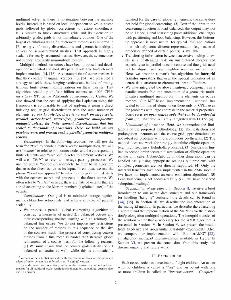
an octant is its front lower left corner (a0 in Figure 1). In order

to perform finite element calculations on octrees, we impose

a restriction on the relative sizes of adjacent octants. This is

also known as the “2:1 balance constraint” (not to be confused

with load balancing): No octant should be more than twice the

size of any other octant that shares a corner, edge, or face with

this octant. This constraint has been used in many other works

as well [6], [8], [14], [17], [18], [24], [38], [39]. In [35], we

presented a parallel algorithm for linear octree construction and

2:1 balancing, which we use in Dendro. Vertices that exist at

the center of a face of an octant are called face-hanging vertices;

vertices that are located at the mid-point of an edge are called

edge-hanging vertices. The 2:1 balance constraint ensures that

there is at most one hanging vertex on any edge or face. In thiswork, we only deal with sorted, complete, linear, 2:1 balancedoctrees.

A pre-processing step for finite element computation is

“meshing”. The construction of the element-to-vertex mappings,the construction of ghost and local vertex lists, and the con-struction of the scatter/gather operators for the near-neighborcommunications that are required during the MatVec are allcomponents of parallel meshing. Our meshing algorithm is

described in [34]. The key features of our meshing algorithm are

that (1) we use a hanging-vertex management scheme (Figure

1) that allows MatVecs in a single tree traversal as opposed to

multiple tree traversal required by the scheme in [38], and (2)we reduce the memory overhead by storing the octree in a com-

pressed form that requires only one byte per octant (used to store

the level of the octant). The element-to-mesh vertex mappings

can be compressed at a modest expense of uncompressing this

on the fly while looping over the elements to perform the finite

element MatVecs. In our hanging-vertex management scheme5,

we do not store hanging vertices explicitly since they do not

represent independent degrees of freedom in a FEM solution.

If the i-th vertex of an element is hanging, then the index

corresponding to this vertex is mapped to the i-th vertex of

the parent6 of this element instead. Thus, if a hanging vertex

is shared between 2 or more elements, then in each element it

might point to a different index. Using this scheme, we construct

4This is not to be confused with the term “multigrid level”.5This scheme is similar to the one used in [39].6The 2:1 balance constraint ensures that the vertices of the parent can never

be hanging.

z

x

y

p1

p4

p2

p3

p5

p6

a4 a5

a7

a6

a0

a1

a2 a3

Fig. 1. Illustration of nodal-connectivities required to perform conforming FEMcalculations using a single tree traversal. All the vertices in this illustrationare labeled in the Morton ordering. Every octant has at least 2 non-hangingvertices, one of which is shared with the parent and the other is shared amongstall the siblings. The octant shown in blue (a) is a child 0, since it sharesits zero vertex (a0) with its parent (p). It shares vertex a7 with its siblings.All other vertices, if hanging, point to the corresponding vertex of the parentoctant instead. Vertices, a3, a5, a6 are face hanging vertices and point top3, p5, p6, respectively. Similarly a1, a2, a4 are edge hanging vertices andpoint to p1, p2, p4.

standard trilinear shape functions with some minor variations:

(1) the shape functions are not rooted at the hanging vertices;

(2) the support of a shape function can spread over more than

8 elements; and (3) if a vertex of an element is hanging, then

the shape functions rooted at the other non-hanging vertices in

that element do not vanish on this hanging vertex. Instead, they

will vanish at the non-hanging vertex that this hanging vertex is

mapped to. In Figure 1 for example, the shape function rooted

at vertex (a0) will not vanish at vertices a1, a2, a3, a4, a5 or a6;

it will vanish at vertices p1, p2, p3, p4, p5, p6 and a7 and assume

a value equal to 1 at vertex a0.

Every octant is owned by a single CPU. The vertices located

at the anchors of the octants are owned by the same CPU that

owns the octants. However, the values of unknowns associated

with octants on inter-CPU boundaries need to be shared among

several CPUs. We keep multiple copies of the information

related to these octants and we term them “ghost” octants. The

elements owned by each CPU are categorized into “indepen-dent” and “dependent” elements. While the elements belonging

to the latter category require ghost information, the elements

belonging to the former category do not. In our implementation

of the finite element MatVec, each CPU iterates over all the

octants it owns and also loops over a layer of ghost octants

that contribute to the vertices it owns.7 Within the loop, each

octant is mapped to one of the 18× 8 hanging configurations8.

This is used to select the appropriate element stencil from a list

of pre-computed stencils. We then use the selected stencil in a

standard element based assembly technique. Although the CPUs

need to read ghost values from other CPUs they only need to

7Each processor only loops over those ghost octants, which are owned byprocessors with ranks less than its own rank. These ghost octants are referredto as “pre-ghosts”.

8Octants could belong to one of 8 child number types and each child numbertype is associated with 18 possible hanging vertex configurations.

3

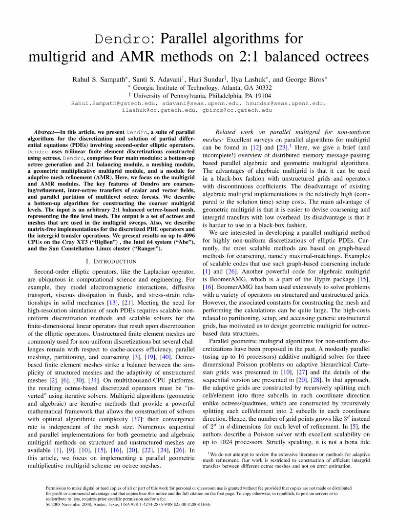
(a) MG Level k − 2 (b) MG Level k − 1 (c) MG Level k

Fig. 2. Quadtree meshes for three successive multigrid (MG) levels.

write data back to the vertices they own and do not need to

write to ghost vertices. Thus, there is only one communication

step within each MatVec. We overlap this communication with

computation corresponding to the independent elements.

III. PARALLEL GEOMETRIC MULTIGRID

The prototypical equation for second-order elliptic operators

is the Poisson problem:

− div(μ(x)∇u(x)) = f(x) ∀x ∈ Ω, u(x) = 0 on ∂Ω.(1)

Here, Ω is the unit cube in three dimensions, ∂Ω is the

boundary of the cube, x is a point in the 3D space, u(x) is

the unknown scalar function, μ(x) is a given scalar function

(commonly referred to as a the “coefficient” for (1)), and

f(x) is a known function. If μ(x) is smooth, (1) can be

efficiently solved with Dendro. If μ is discontinuous, we can

still use Dendro but the convergence rates may be suboptimal.9

We write the discretized finite-dimensional system of linear

equations as Akuk = fk, where k denotes the multigrid level.

The Dendro interface: Let us describe the Dendro inter-

face for (1). (The current implementation of Dendro supports

more general scalar equations, vector equations such as the

linear elastostatics equation10, and time-dependent parabolic,

and hyperbolic equations.) The input is μ, f , boundary con-

ditions, and a list of target points in which we want to evaluate

the solution. The output is the solution u and, optionally, its

gradient at the target points. For simplicity, we assume the

following representation for μ: it is approximated as the sum

of a constant (background or base value) plus a function that

is defined by specifying its value on a set of points. f is

represented in a similar manner. We assume that the lists of

points that are used to specify μ and f are distributed arbitrarily

across CPUs. Dendro uses these points to define an octree at

the finest multigrid level and subsequently uses the fine level

octree to bottom-up construct the multigrid hierarchy. Next,

we give details about the main algorithmic components of this

procedure.

9The current Dendro implementation supports isotropic problems only. Weare working on extending Dendro to anisotropic operators in which μ(x) is atensor.

10The elastostatics equation is given by div(μ(x)∇v(x)) + ∇(λ(x) +μ(x))∇v(x)) = b(x), where μ and λ are scalar fields known as Lame moduli;and v and b are 3D vector functions.

Outline of the Dendro algorithms: In Dendro, we use

a hierarchy of octrees (see Figure 2), which we construct

as part of the geometric multigrid (GMG) V-cycle algorithm.

The V-cycle algorithm consists of 6 main steps: (1) Pre-

smoothing: uk = Sk(uk, fk, Ak); (2) Residual computation:

rk = fk −Akuk; (3) Restriction: rk−1 = Rkrk; (4) Recursion:

ek−1=GMG(Ak−1, rk−1); (5) Prolongation: uk = uk +Pkek−1;

and (6) Post-smoothing: uk = Sk(uk, fk, Ak). When “k”

reaches the coarsest multigrid level, which we term the “exactsolve” level, we solve for ek exactly using a single level solver

(e.g., a parallel sparse direct factorization method).

To setup the solver we start with user specified points for μand f and follow the following steps:

1) Given input points, construct a 2:1 balanced octree corre-

sponding to the finest multigrid level using the algorithms

described in [35].

2) Given an upper bound on the total number of multigrid

levels, construct the sequence of coarser octrees.

3) Mesh the octrees starting with the octree corresponding

to the coarsest multigrid level.

4) Construct restriction and prolongation operators between

successive multigrid levels.

In the following sections, we describe the various components

of the multigrid algorithm.

A. Global coarsening

Starting with the finest octree, we iteratively construct a

hierarchy of complete, balanced, linear octrees such that every

octant in the k-th octree (coarse) is either present in the k+1-th

octree (fine) as well or all its eight children are present instead

(Figure 2).

We construct the k-th octree from the k + 1-th octree by

replacing every set of eight siblings by their parent. This is an

operation with O(N) work complexity, where N is the number

of leaves in the k +1-th octree. It is easy to parallelize and has

an O( Nnp

) parallel time complexity, where np is the number of

CPUs.11 The main parallel operations are two circular shifts;

one clockwise and another anti-clockwise.

However, the operation described above may produce 4:1

balanced octrees12 instead of 2:1 balanced octrees. Although

there is only one level of imbalance that we need to correct, the

imbalance can still affect octants that are not in its immediate

vicinity. This is known as the ripple effect. Even with just one

level of imbalance, a ripple can still propagate across many

CPUs.

The sequence of octrees constructed as described above has

the property that non-hanging vertices in any octree remain non-

hanging in all finer octrees as well. Hanging vertices on any

octree could either become non-hanging on a finer octree or

remain hanging on the finer octrees too. In addition, an octree

can have new hanging as well as non-hanging vertices that are

not present in any of the coarser octrees.

11When we discuss communication costs we assume a Hypercube networktopology with θ(np) bandwidth.

12The input is 2:1 balanced and we coarsen by at most one level in thisoperation. Hence, this operation will only introduce one additional level ofimbalance resulting in 4:1 balanced octrees.

4

B. Restriction and Prolongation operators

To implement the intergrid transfer operations, we need to

find all the non-hanging fine grid vertices that lie within the

support of each coarse grid shape function. These operations

can be implemented quite efficiently for the hierarchy of the

octree meshes constructed as described in Section III-A. We do

not construct these matrices explicitly, instead we implement

a matrix-free scheme using MatVecs as described below. The

MatVecs for the restriction and prolongation operators are

similar.13 In both the MatVecs, we loop over the coarse and

fine grid octants simultaneously. For each coarse-grid octant,

the underlying fine-grid octant could either be identical to the

coarse octant or one of its eight children. We identify these

cases and handle them separately. The main operation within

the loop is selecting the coarse-grid shape functions that do

not vanish within the current coarse-grid octant and evaluating

them at the non-hanging fine-grid vertices that lie within this

coarse-grid octant. These form the entries of the restriction and

prolongation matrices.

To be able to do this operation efficiently in parallel, we need

the coarse and fine grid partitions to be aligned. This means that

the following two conditions must be satisfied. (1) If an octantexists both in the coarse and fine grids, then the same CPU must“own” this octant on both the meshes; and (2) If an octant’schildren exist in the fine grid, then the same CPU must ownthis octant on the coarse mesh and all its 8 children on the finemesh.

To satisfy these conditions, we first compute the partition on

the coarse grid and then impose it on the finer grid. In general,

it might not be possible or desirable to use the same partition

for all of the multigrid levels because using the same partition

for all the levels could cause load imbalance. Also, the coarse

levels may be too sparse to be distributed across all of the

CPUs. For these reasons, we allow different partitioning across

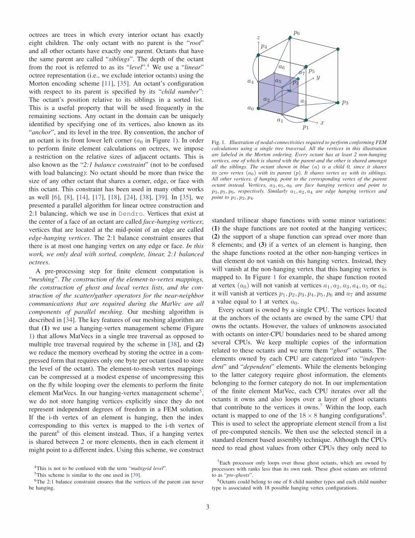
levels. 14 When a transition in the partitions is required, we

duplicate the octree at the multigrid level at which the transition

between different partitioning takes place and we let one of

the duplicates share its partitioning with its immediate finer

level and the other one share its partitioning with its immediate

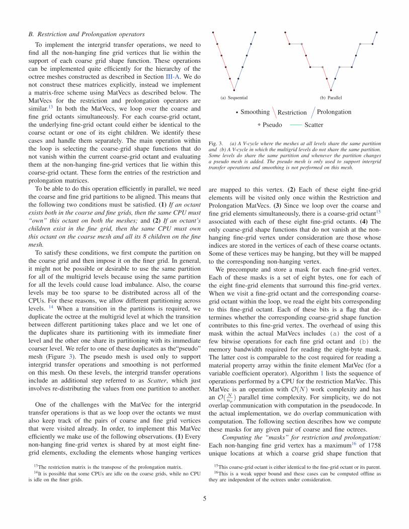
coarser level. We refer to one of these duplicates as the“pseudo”

mesh (Figure 3). The pseudo mesh is used only to support

intergrid transfer operations and smoothing is not performed

on this mesh. On these levels, the intergrid transfer operations

include an additional step referred to as Scatter, which just

involves re-distributing the values from one partition to another.

One of the challenges with the MatVec for the intergrid

transfer operations is that as we loop over the octants we must

also keep track of the pairs of coarse and fine grid vertices

that were visited already. In order, to implement this MatVec

efficiently we make use of the following observations. (1) Every

non-hanging fine-grid vertex is shared by at most eight fine-

grid elements, excluding the elements whose hanging vertices

13The restriction matrix is the transpose of the prolongation matrix.14It is possible that some CPUs are idle on the coarse grids, while no CPU

is idle on the finer grids.

(a) Sequential (b) Parallel

Smoothing Restriction Prolongation

Pseudo Scatter

Fig. 3. (a) A V-cycle where the meshes at all levels share the same partitionand (b) A V-cycle in which the multigrid levels do not share the same partition.Some levels do share the same partition and whenever the partition changesa pseudo mesh is added. The pseudo mesh is only used to support intergridtransfer operations and smoothing is not performed on this mesh.

are mapped to this vertex. (2) Each of these eight fine-grid

elements will be visited only once within the Restriction and

Prolongation MatVecs. (3) Since we loop over the coarse and

fine grid elements simultaneously, there is a coarse-grid octant15

associated with each of these eight fine-grid octants. (4) The

only coarse-grid shape functions that do not vanish at the non-

hanging fine-grid vertex under consideration are those whose

indices are stored in the vertices of each of these coarse octants.

Some of these vertices may be hanging, but they will be mapped

to the corresponding non-hanging vertex.

We precompute and store a mask for each fine-grid vertex.

Each of these masks is a set of eight bytes, one for each of

the eight fine-grid elements that surround this fine-grid vertex.

When we visit a fine-grid octant and the corresponding coarse-

grid octant within the loop, we read the eight bits corresponding

to this fine-grid octant. Each of these bits is a flag that de-

termines whether the corresponding coarse-grid shape function

contributes to this fine-grid vertex. The overhead of using this

mask within the actual MatVecs includes (a) the cost of a

few bitwise operations for each fine grid octant and (b) the

memory bandwidth required for reading the eight-byte mask.

The latter cost is comparable to the cost required for reading a

material property array within the finite element MatVec (for a

variable coefficient operator). Algorithm 1 lists the sequence of

operations performed by a CPU for the restriction MatVec. This

MatVec is an operation with O(N) work complexity and has

an O( Nnp

) parallel time complexity. For simplicity, we do not

overlap communication with computation in the pseudocode. In

the actual implementation, we do overlap communication with

computation. The following section describes how we compute

these masks for any given pair of coarse and fine octrees.

Computing the “masks” for restriction and prolongation:Each non-hanging fine grid vertex has a maximum16 of 1758

unique locations at which a coarse grid shape function that

15This coarse-grid octant is either identical to the fine-grid octant or its parent.16This is a weak upper bound and these cases can be computed offline as

they are independent of the octrees under consideration.

5

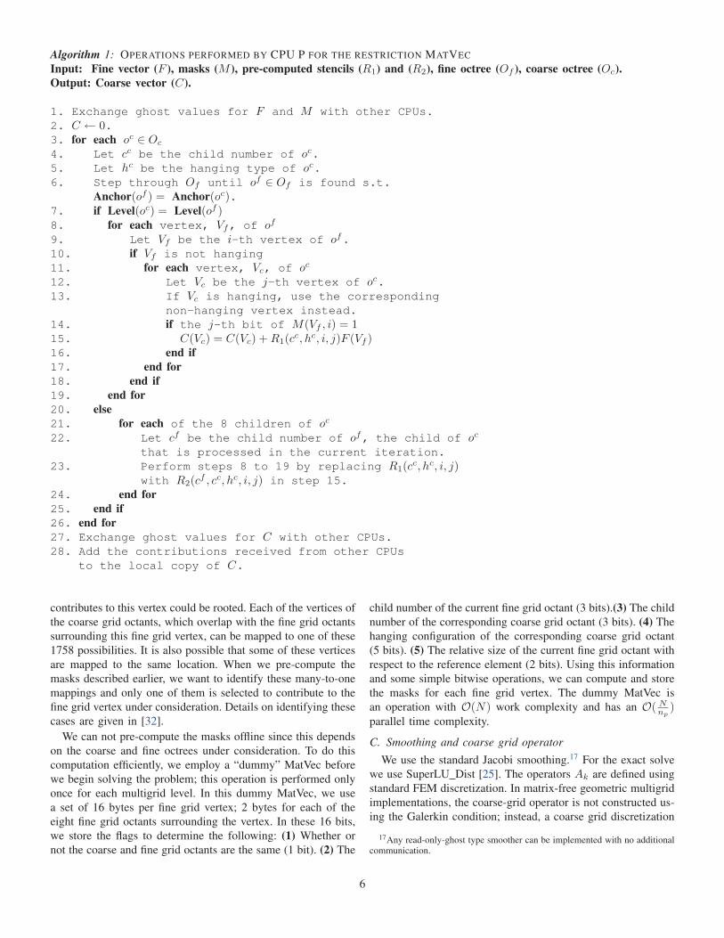
Algorithm 1: OPERATIONS PERFORMED BY CPU P FOR THE RESTRICTION MATVEC

Input: Fine vector (F ), masks (M ), pre-computed stencils (R1) and (R2), fine octree (Of ), coarse octree (Oc).Output: Coarse vector (C).

1. Exchange ghost values for F and M with other CPUs.2. C ← 0.3. for each oc ∈ Oc

4. Let cc be the child number of oc.5. Let hc be the hanging type of oc.6. Step through Of until of ∈ Of is found s.t.

Anchor(of ) = Anchor(oc).7. if Level(oc) = Level(of )8. for each vertex, Vf, of of

9. Let Vf be the i-th vertex of of.10. if Vf is not hanging11. for each vertex, Vc, of oc

12. Let Vc be the j-th vertex of oc.13. If Vc is hanging, use the corresponding

non-hanging vertex instead.14. if the j-th bit of M(Vf , i) = 115. C(Vc) = C(Vc) + R1(cc, hc, i, j)F (Vf )16. end if17. end for18. end if19. end for20. else21. for each of the 8 children of oc

22. Let cf be the child number of of, the child of oc

that is processed in the current iteration.23. Perform steps 8 to 19 by replacing R1(cc, hc, i, j)

with R2(cf , cc, hc, i, j) in step 15.24. end for25. end if26. end for27. Exchange ghost values for C with other CPUs.28. Add the contributions received from other CPUs

to the local copy of C.

contributes to this vertex could be rooted. Each of the vertices of

the coarse grid octants, which overlap with the fine grid octants

surrounding this fine grid vertex, can be mapped to one of these

1758 possibilities. It is also possible that some of these vertices

are mapped to the same location. When we pre-compute the

masks described earlier, we want to identify these many-to-one

mappings and only one of them is selected to contribute to the

fine grid vertex under consideration. Details on identifying these

cases are given in [32].

We can not pre-compute the masks offline since this depends

on the coarse and fine octrees under consideration. To do this

computation efficiently, we employ a “dummy” MatVec before

we begin solving the problem; this operation is performed only

once for each multigrid level. In this dummy MatVec, we use

a set of 16 bytes per fine grid vertex; 2 bytes for each of the

eight fine grid octants surrounding the vertex. In these 16 bits,

we store the flags to determine the following: (1) Whether or

not the coarse and fine grid octants are the same (1 bit). (2) The

child number of the current fine grid octant (3 bits).(3) The child

number of the corresponding coarse grid octant (3 bits). (4) The

hanging configuration of the corresponding coarse grid octant

(5 bits). (5) The relative size of the current fine grid octant with

respect to the reference element (2 bits). Using this information

and some simple bitwise operations, we can compute and store

the masks for each fine grid vertex. The dummy MatVec is

an operation with O(N) work complexity and has an O( Nnp

)parallel time complexity.

C. Smoothing and coarse grid operator

We use the standard Jacobi smoothing.17 For the exact solve

we use SuperLU Dist [25]. The operators Ak are defined using

standard FEM discretization. In matrix-free geometric multigrid

implementations, the coarse-grid operator is not constructed us-

ing the Galerkin condition; instead, a coarse grid discretization

17Any read-only-ghost type smoother can be implemented with no additionalcommunication.

6

of the underlying PDE is used. One can show [32] that these

two formulations are equivalent provided the same bilinear form,

a(u, v), is used both on the coarse and fine levels. This poses

no difficulty for constant coefficient problems or problems in

which the material property is described in a closed form. Most

often however, the material property is defined just on each

fine-grid element. Hence, the bilinear form actually depends on

the discretization used. If the coarser grids must use the same

bilinear form, the coarser grid MatVecs must be performed by

looping over the underlying finest grid elements, using the mate-

rial property defined on each fine grid element. This would make

the coarse grid MatVecs quite expensive. A cheaper alternative

would be to define the material properties for the coarser grid

elements as the average of those for the underlying fine grid

elements. This process amounts to using a different bilinear

form for each multigrid level and hence is a clear deviation

from the theory. This is one reason why the convergence of

the stand-alone multigrid solver deteriorates with increasing

contrast in material properties. Coarsening across discontinuities

also affects the coarse grid correction, even when the Galerkin

condition is satisfied. Large contrasts in material properties also

affect simple smoothers like the Jacobi smoother. The standard

solution is to use multigrid as a preconditioner to the Conjugate

Gradient (CG) method [37]. We have conducted numerical

experiments that demonstrate the effectiveness of this approach

for the Poisson problem.

D. Metric for load imbalance

In all our MatVecs, the communication cost is proportional

to the number of inter-CPU dependent elements and the com-

putation cost is proportional to the total number of local and

pre-ghost elements (Section II). We use the following heuristic

to estimate the local load on any processor at any given multigrid

level:

Local Load = 0.75 × (No. of local elements + (2)

No. of pre-ghost elements) +0.25 × (No. of dependent elements)

Then, the load imbalance for that multigrid level is computed

as the ratio of the maximum and minimum local loads across

the processors.

E. Summary of the overall multigrid algorithm

1) A “sufficiently” fine18 2:1 balanced complete linear octree

is constructed using the algorithms described in [35].

2) Starting with the finest octree, a sequence of 2:1 balanced

coarse linear octrees is constructed using the global coars-

ening algorithm.

3) The maximum number of processors that can be used for

each multigrid level without violating the minimum grain

18Here the term sufficiently is used to mean that the discretization errorintroduced is acceptable.

size criteria19 is computed.

4) Starting with the coarsest octree, the octree at each level

is meshed using the algorithm described in [34]. As long

as the load imbalance (Section III-D) across the CPUs is

acceptable and as long as the number of CPUs used for

the coarser grid is the same as the maximum number of

CPUs that can be used for the finer multigrid level without

violating the minimum grain size criteria, the partition of

the coarser grid is imposed on to the finer grid during

meshing. If either of the above two conditions is violated

then the octree for the finer grid is duplicated; One of

them is meshed using the partition of the coarser grid and

the other is meshed using a fresh partition computed using

the “Block Partition” algorithm [34], [35]. The process is

repeated until the finest octree has been meshed.

5) A dummy restriction MatVec (Section III-B) is performed

at each level (except the coarsest) and the masks that will

be used in the actual restriction and prolongation MatVecs

are computed and stored.

6) For the case of variable coefficient operators, vectors that

store the material properties at each level are created.

7) The discrete system of equations is then solved using

the conjugate gradient algorithm preconditioned with the

multigrid scheme.

Complexity: Let N be the total number of octants in the

fine level and np be the number of CPUs. In [34] and [35], we

showed that the parallel complexity of the single-level construc-

tion, 2:1 balancing and meshing is O( Nnp

log Nnp

+ np log np)for trees that are nearly uniform. The cost of a MatVec is

O( Nnp

). The complexity of a single-level coarsening (excluding

2:1 balancing) is O( Nnp

).

IV. ADAPTIVE MESH REFINEMENT

We solve a linear parabolic problem: ∂u∂t = Δu+f(x, t) with

homogeneous Neumann boundary conditions using adaptive

mesh refinement. We compute f(x, t) using an analytical solu-

tion of a traveling wave of the form u(x, t) = exp(−104(y −0.5 − 0.1t − 0.1 sin(2πx))2) (see Figure 6). A second order

implicit Crank-Nicholson scheme is used to solve the problem

for 10 time steps with a step size of δt = 0.05. We used CG with

Jacobi preconditioner to solve the linear system of discretized

equations at every time step. We build the octree using the exact

analytical solution. We do not use any error estimator. We focus

on demonstrating the performance of our tree-construction,

balancing, meshing and solution transfer schemes. Below we

describe the adaptive mesh refinement scheme.

1) Coarsen or refine octants in an octree using the exact

analytical solution at the current time step.

2) Balance the octree to enforce the 2:1 balance constraint.

19We require a minimum of 1000 elements per processor for good scalability.If this criteria is not satisfied for any particular multigrid level, then the numberof active processors for that level is automatically adjusted. We arrived at thisnumber by assuming an uniform distribution of elements and comparing thenumber of elements in the interior of a processor and the number of elementson the inter-processor surface. The number of elements in the interior of aprocessor must be much greater than the number of elements on the inter-processor surface for good scalability.

7

3) Mesh the octree to get the element-vertex connectivity.

4) Transfer the solution at the previous time step to the new

mesh.

5) Solve the linear system of equations.

We also present a parallel algorithm to map the solutionbetween different multigrid levels .

1) Get the list of co-ordinates of the vertices in the new mesh

O(N/np).2) Sort the list of co-ordinates using parallel sample sort.

O(N/np log(N/np) + np log np).3) Impose the partition of the old mesh on the sorted list

O(N/np).4) Evaluate the function values at the vertices of the new

mesh using the nodal values and shape functions of the

old mesh O(N/np).5) Re-distribute the evaluated function values to the partition

of the new mesh O(N/np).The overall computational complexity of the solution transfer

algorithm, assuming that the octrees have O(N) vertices and

are similar, is O(N/np + np log np). We do not require the

meshes at two different time steps to be aligned or to share the

same partition. In fact, the two meshes can be entirely different.

Of course, the greater their differences the higher the intergrid

transfer communication costs.

V. NUMERICAL EXPERIMENTS

In this section, we report the results from four sets of ex-

periments: (A) Isogranular scalability (weak scaling) for multi-

grid, (B) Fixed-size scalability (strong scaling) for multigrid,

(C) Comparison between Dendro and BoomerAMG and (D)

Isogranular scalability for AMR. The experiments were carried

out on the Teragrid systems: “Abe” (9.2K Intel-Woodcrest cores

with Infiniband), “Bigben” (4.1K AMD Opteron cores with

quadrics) and “Ranger” (63K Barcelona cores with Infiniband).

Details for these systems can be found in [29], [31], [36]. The

following parameters were used in experiments A, B and C: (1)A zero initial guess was used, (2) SuperLU_dist [25] was

used as an exact solver at the coarsest grid, (3) the forcing term

was computed by using a random vector for the exact solution,

(4) one multigrid V-cycle with 4 pre-smoothing and 4 post-

smoothing steps per level was used as a preconditioner to the

Conjugate Gradient (CG) method and (5) the damped-Jacobi

method was used as the smoother at each multigrid level.

Isogranular scalability analysis was performed by roughly

keeping the problem size per CPU fixed while increasing

the number of CPUs. Fixed-size scalability was performed by

keeping the problem size constant while increasing the number

of CPUs. In all of the fixed-size and isogranular scalability

plots, the first column reports the total setup time, the second

column gives the component-wise split-up of the total setup

time. The third column represents the total solve time and the

last column gives the component-wise split-up for the solve

phase. Note that the reported times for each component are the

maximum values for that component across all the processors.

Hence, in some cases the total time is lower than the sum of

the individual components. The setup cost for the GMG scheme

(Dendro) includes the time for constructing the mesh for all

the levels (including the finest), constructing and balancing all

the coarser levels, setting up the intergrid transfer operators by

performing one dummy restriction MatVec at each level. The

time to create the work vectors for the MG scheme and the

time to build the coarsest grid matrix are also included in the

total setup time, but are not reported individually since they are

insignificant. “Scatter” refers to the process of transferring the

vectors between two different partitions of the same multigrid

level during the intergrid transfer operations, required whenever

the coarse and fine grids do not share the same partition. The

time spent in applying the Jacobi preconditioner, computing the

inner-products within CG and solving the coarsest grid problems

using LU are all accounted for in the total solve time, but are

not reported individually since they are insignificant. When we

report MPI_Wait() times, we refer to synchronization for

non-blocking operations during the “Solve” phase.

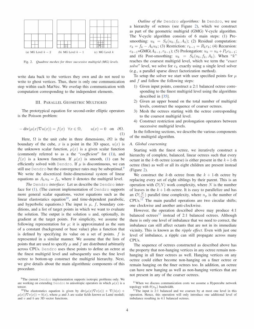
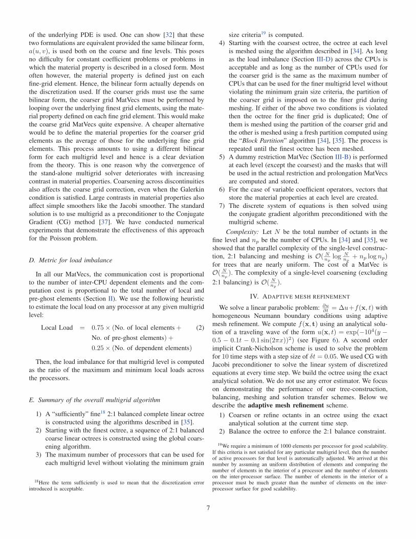
Isogranular scalability for the multigrid solver: In Figure

4(a), we report isogranular scalability results for the constant-

coefficient scalar Poisson problem with homogeneous Neumann

boundary conditions on meshes whose mesh-size follows a

Gaussian distribution. The finest level octrees for the multiple

CPU cases were generated using regular refinements from the

finest octree for the single CPU case. Hence, the number of

elements on the finest multigrid level grows exactly by a factor

of 8 every time the number of CPUs is increased by a factor of

8. 4 multigrid levels were used on 1 CPU and the number of

multigrid levels were incremented by 1 every time the number

of CPUs is increased by a factor of 8. For all the multi-

processor runs in this experiment, the coarsest level only used

3 processors.

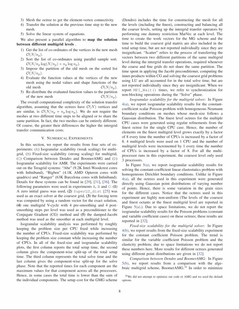
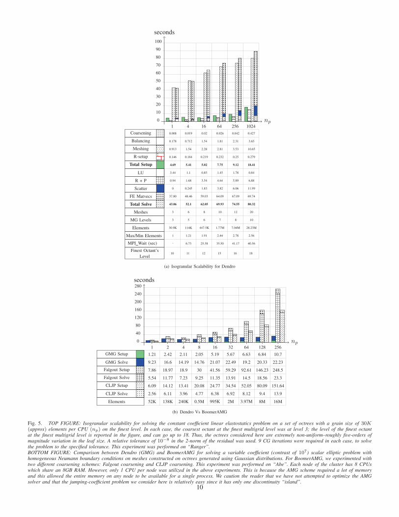
In Figure 5(a), we report isogranular scalability results for

solving the constant-coefficient linear elastostatics problem with

homogeneous Dirichlet boundary conditions. Unlike in Figure

4(a), all the octrees used in this experiment were generated

directly using Gaussian point distributions of varying number

of points. Hence, there is some variation in the grain sizes

for the different cases. Notice that the octrees used in this

experiment are highly non-uniform (The levels of the coarsest

and finest octants at the finest multigrid level are reported in

Figure 5(a).). Due to space limitations, we do not report the

isogranular scalability results for the Poisson problems (constant

and variable coefficient cases) on these octrees; these results are

reported in [32].

Fixed-size scalability for the multigrid solver: In Figure

4(b), we report results from the fixed-size scalability experiment

for the constant coefficient Poisson problem. The trend is

similar for the variable coefficient Poisson problem and the

elasticity problem; due to space limitations we do not report

these numbers here. More results for different octrees generated

using different point distributions are given in [32].

Comparison between Dendro and BoomerAMG: In Figure

5(b), we report results from a comparison with the alge-

braic multigrid scheme, BoomerAMG.20 In order to minimize

20We did not attempt to optimize our code or AMG and we used the defaultoptions.

8

np

seconds

1 8 64 512 4096

0

25

50

75

100

125

150

175

200

225

Coarsening

Balancing

Meshing

R-setup

Total Setup

LU

R + P

Scatter

FE Matvecs

Total Solve

Meshes

MG Levels

Max/Min Elements

MPI Wait (sec)

0.046

0.52

4.39

0.929

6.01

0.539

2.89

0

31.41

35.07

4

4

1

-

0.098

1.19

5.35

0.906

7.74

0.283

11.05

0.215

96.45

100.76

6

5

1.14

49.42

0.099

2.11

7.66

1.34

11.63

0.283

11.0

0.6

60.53

65.5

9

6

1.77

28.14

0.145

2.19

17.65

1.3

22.4

0.294

6.16

32.22

110.16

115.73

13

7

2.59

62.0

0.874

4.0

37.48

1.46

47.86

0.284

6.61

57.81

151.33

164.29

15

8

2.64

93.40

(a) Isogranular Scalability

np

seconds

32 64 128 256 512 1024

0

40

80

120

160

200

240

280

320

360

400

Coarsening

Balancing

Meshing

R-setup

Total Setup

LU

R + P

Scatter

FE Matvecs

Total Solve

Meshes

0.201

3.25

12.98

2.50

19.30

0.282

61.01

0.905

312.64

326.44

8

0.098

2.28

8.28

1.36

12.47

0.284

19.63

0.934

100.1

108.3

9

0.059

1.27

4.96

0.65

7.37

0.284

10.2

1.62

51.22

56.89

9

0.048

0.85

3.89

0.36

5.67

0.285

4.87

14.46

24.74

28.93

10

0.054

0.71

2.82

0.198

4.33

0.284

2.31

2.8

10.76

13.97

10

0.089

0.67

3.42

0.132

4.90

0.282

1.32

5.98

9.56

13.26

11

(b) Fixed-size Scalability

Fig. 4. LEFT FIGURE: Isogranular scalability for solving the constant coefficient Poisson problem on a set of octrees with a grain size of 239.4K elements perCPU (np) on the finest level. The difference between the minimum and maximum levels of the octants on the finest grid is 5. A relative tolerance of 10−10 inthe 2-norm of the residual was used. 6 CG iterations were required in each case, to solve the problem to the specified tolerance. This experiment was performedon “Bigben”.RIGHT FIGURE: Scalability for a fixed fine grid problem size of 15.3M elements. The problem is the same as described in Figure 4(a). 6 multigrid levels wereused. 9 iterations were required to solve the problem to a relative tolerance of 10−14 in the 2-norm of the residual. This experiment was performed on “Bigben”.

communication costs, the coarsest level was distributed on a

maximum of 32 CPUs in all experiments. For BoomerAMG, we

experimented with two different coarsening schemes: Falgout

coarsening and CLJP coarsening. The results from both experi-

ments are reported. Falgout coarsening works best for structured

grids and CLJP coarsening is better suited for unstructured

grids [22]. We compare our results using both the schemes.

Both GMG and AMG schemes used 4 pre-smoothing steps

and 4 post-smoothing steps per level with the damped Jacobi

smoother. A relative tolerance of 10−10 in the 2-norm of the

residual was used in all the cases. The GMG scheme took about

12 CG iterations, the Falgout scheme took about 7 iterations and

the CLJP scheme also took about 7 iterations.

The setup time reported for the AMG schemes includes the

time for meshing the finest grid and constructing the finest grid

FE matrix, both of which are quite small (≈ 1.35 seconds for

meshing and ≈ 22.93 seconds for building the fine grid matrix

even on 256 CPUs) compared to the time to setup the rest of

the AMG scheme. Although GMG seems to be performing well,

more difficult problems with multiple discontinuous coefficients

can cause it to fail. Our method is not robust in the presence ofdiscontinuous coefficients—in contrast to AMG.

Discussion on scalability results: The setup costs are

much smaller than the solution costs, suggesting that Dendrois

suitable for problems that require the construction and solution

of linear systems of equations numerous times. The increase

in running times for the large processor cases can be primarily

attributed to poor load balancing. This can be seen from (a) the

total time spent in calls to the MPI_Wait() function and (b)the imbalance in the number of elements (own + pre-ghosts)

per processor. These numbers are reported in Figure 4(a) and

Figure 5(a).21 Load balancing is a challenging problem due to

the following reasons: (1) We need to make an accurate a-

priori estimate of the computation and communication loads–it

is difficult to make such estimates for arbitrary distributions;

(2) for the intergrid transfer operations, the coarse and fine

grids need to be aligned-it is difficult to get good load balance

for both the grids, especially for non-uniform distributions; and

(3) Partioning each multigrid level independently to get good

load balance for the smoothing operations at each multigrid

level would require the creation of an auxiliary mesh for each

multigrid level and a scatter operation for each intergrid transfer

21We only report the Max/Min elements ratios for the finest multigrid levelalthough the trend is similar for other levels as well.

9

np

seconds

1 4 16 64 256 1024

0

10

20

30

40

50

60

70

80

90

100

Coarsening

Balancing

Meshing

R-setup

Total Setup

LU

R + P

Scatter

FE Matvecs

Total Solve

Meshes

MG Levels

Elements

Max/Min Elements

MPI Wait (sec)

Finest Octant’s

Level

0.008

0.178

0.913

0.146

4.69

3.44

0.94

0

37.80

43.06

3

3

30.9K

1

-

10

0.019

0.712

1.54

0.184

5.41

1.1

1.68

0.245

48.46

52.1

6

5

114K

1.21

6.73

11

0.02

1.54

2.28

0.219

5.02

0.85

3.54

1.83

59.03

62.05

8

6

447.5K

1.91

25.58

12

0.026

1.81

2.81

0.232

7.75

1.45

4.64

3.82

64.09

69.93

10

7

1.77M

2.44

35.50

15

0.042

2.31

3.53

0.25

9.12

1.78

5.89

6.06

67.09

74.55

12

8

7.04M

2.78

41.17

16

0.427

3.65

10.65

0.279

18.41

0.84

6.88

11.99

69.74

80.32

20

10

28.23M

2.56

40.56

18

(a) Isogranular Scalability for Dendro

np

seconds

1 2 4 8 16 32 64 128 256

0

40

80

120

160

200

240

280

GMG Setup

GMG Solve

Falgout Setup

Falgout Solve

CLJP Setup

CLJP Solve

Elements

1.21

9.23

7.86

5.54

6.09

2.56

52K

2.42

16.6

18.97

11.77

14.12

6.11

138K

2.11

14.19

18.9

7.23

13.41

3.96

240K

2.05

14.76

30

9.25

20.08

4.77

0.5M

5.19

21.07

41.56

11.35

24.77

6.38

995K

5.67

22.49

59.29

13.91

34.54

6.92

2M

6.63

19.2

92.61

14.5

52.05

8.12

3.97M

6.84

20.33

146.23

18.56

80.09

9.4

8M

10.7

22.23

248.5

23.3

151.64

13.9

16M

(b) Dendro Vs BoomerAMG

Fig. 5. TOP FIGURE: Isogranular scalability for solving the constant coefficient linear elastostatics problem on a set of octrees with a grain size of 30K(approx) elements per CPU (np) on the finest level. In each case, the coarsest octant at the finest multigrid level was at level 3; the level of the finest octantat the finest multigrid level is reported in the figure, and can go up to 18. Thus, the octrees considered here are extremely non-uniform–roughly five-orders ofmagnitude variation in the leaf size. A relative tolerance of 10−8 in the 2-norm of the residual was used. 9 CG iterations were required in each case, to solvethe problem to the specified tolerance. This experiment was performed on “Ranger”.BOTTOM FIGURE: Comparison between Dendro (GMG) and BoomerAMG for solving a variable coefficient (contrast of 107) scalar elliptic problem withhomogeneous Neumann boundary conditions on meshes constructed on octrees generated using Gaussian distributions. For BoomerAMG, we experimented withtwo different coarsening schemes: Falgout coarsening and CLJP coarsening. This experiment was performed on “Abe”. Each node of the cluster has 8 CPUswhich share an 8GB RAM. However, only 1 CPU per node was utilized in the above experiments. This is because the AMG scheme required a lot of memoryand this allowed the entire memory on any node to be available for a single process. We caution the reader that we have not attempted to optimize the AMGsolver and that the jumping-coefficient problem we consider here is relatively easy since it has only one discontinuity “island”.

10

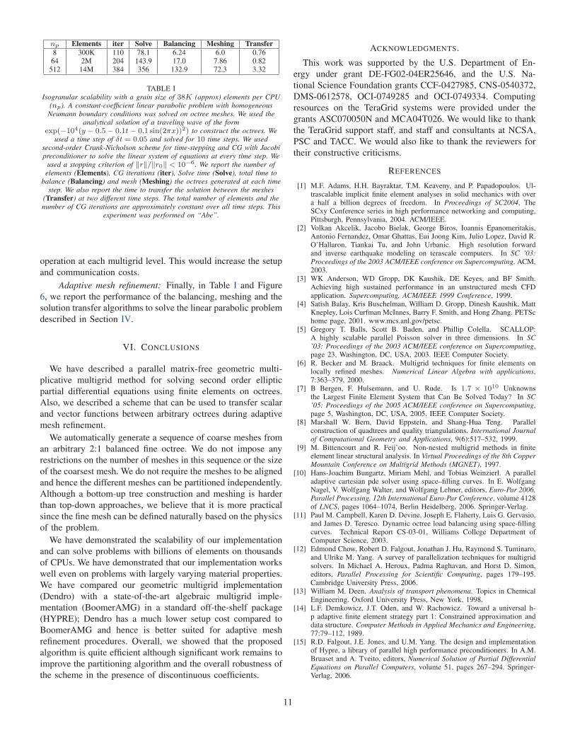
np Elements iter Solve Balancing Meshing Transfer8 300K 110 78.1 6.24 6.0 0.7664 2M 204 143.9 17.0 7.86 0.82

512 14M 384 356 132.9 72.3 3.32

TABLE IIsogranular scalability with a grain size of 38K (approx) elements per CPU

(np). A constant-coefficient linear parabolic problem with homogeneousNeumann boundary conditions was solved on octree meshes. We used the

analytical solution of a traveling wave of the formexp(−104(y − 0.5 − 0.1t − 0.1 sin(2πx))2) to construct the octrees. We

used a time step of δt = 0.05 and solved for 10 time steps. We usedsecond-order Crank-Nicholson scheme for time-stepping and CG with Jacobipreconditioner to solve the linear system of equations at every time step. We

used a stopping criterion of ‖r‖/‖r0‖ < 10−6. We report the number ofelements (Elements), CG iterations (iter), Solve time (Solve), total time to

balance (Balancing) and mesh (Meshing) the octrees generated at each timestep. We also report the time to transfer the solution between the meshes

(Transfer) at two different time steps. The total number of elements and thenumber of CG iterations are approximately constant over all time steps. This

experiment was performed on “Abe”.

operation at each multigrid level. This would increase the setup

and communication costs.

Adaptive mesh refinement: Finally, in Table I and Figure

6, we report the performance of the balancing, meshing and the

solution transfer algorithms to solve the linear parabolic problem

described in Section IV.

VI. CONCLUSIONS

We have described a parallel matrix-free geometric multi-

plicative multigrid method for solving second order elliptic

partial differential equations using finite elements on octrees.

Also, we described a scheme that can be used to transfer scalar

and vector functions between arbitrary octrees during adaptive

mesh refinement.

We automatically generate a sequence of coarse meshes from

an arbitrary 2:1 balanced fine octree. We do not impose any

restrictions on the number of meshes in this sequence or the size

of the coarsest mesh. We do not require the meshes to be aligned

and hence the different meshes can be partitioned independently.

Although a bottom-up tree construction and meshing is harder

than top-down approaches, we believe that it is more practical

since the fine mesh can be defined naturally based on the physics

of the problem.

We have demonstrated the scalability of our implementation

and can solve problems with billions of elements on thousands

of CPUs. We have demonstrated that our implementation works

well even on problems with largely varying material properties.

We have compared our geometric multigrid implementation

(Dendro) with a state-of-the-art algebraic multigrid imple-

mentation (BoomerAMG) in a standard off-the-shelf package

(HYPRE); Dendro has a much lower setup cost compared to

BoomerAMG and hence is better suited for adaptive mesh

refinement procedures. Overall, we showed that the proposed

algorithm is quite efficient although significant work remains to

improve the partitioning algorithm and the overall robustness of

the scheme in the presence of discontinuous coefficients.

ACKNOWLEDGMENTS.

This work was supported by the U.S. Department of En-

ergy under grant DE-FG02-04ER25646, and the U.S. Na-

tional Science Foundation grants CCF-0427985, CNS-0540372,

DMS-0612578, OCI-0749285 and OCI-0749334. Computing

resources on the TeraGrid systems were provided under the

grants ASC070050N and MCA04T026. We would like to thank

the TeraGrid support staff, and staff and consultants at NCSA,

PSC and TACC. We would also like to thank the reviewers for

their constructive criticisms.

REFERENCES

[1] M.F. Adams, H.H. Bayraktar, T.M. Keaveny, and P. Papadopoulos. Ul-trascalable implicit finite element analyses in solid mechanics with overa half a billion degrees of freedom. In Proceedings of SC2004, TheSCxy Conference series in high performance networking and computing,Pittsburgh, Pennsylvania, 2004. ACM/IEEE.

[2] Volkan Akcelik, Jacobo Bielak, George Biros, Ioannis Epanomeritakis,Antonio Fernandez, Omar Ghattas, Eui Joong Kim, Julio Lopez, David R.O’Hallaron, Tiankai Tu, and John Urbanic. High resolution forwardand inverse earthquake modeling on terascale computers. In SC ’03:Proceedings of the 2003 ACM/IEEE conference on Supercomputing. ACM,2003.

[3] WK Anderson, WD Gropp, DK Kaushik, DE Keyes, and BF Smith.Achieving high sustained performance in an unstructured mesh CFDapplication. Supercomputing, ACM/IEEE 1999 Conference, 1999.

[4] Satish Balay, Kris Buschelman, William D. Gropp, Dinesh Kaushik, MattKnepley, Lois Curfman McInnes, Barry F. Smith, and Hong Zhang. PETSchome page, 2001. www.mcs.anl.gov/petsc.

[5] Gregory T. Balls, Scott B. Baden, and Phillip Colella. SCALLOP:A highly scalable parallel Poisson solver in three dimensions. In SC’03: Proceedings of the 2003 ACM/IEEE conference on Supercomputing,page 23, Washington, DC, USA, 2003. IEEE Computer Society.

[6] R. Becker and M. Braack. Multigrid techniques for finite elements onlocally refined meshes. Numerical Linear Algebra with applications,7:363–379, 2000.

[7] B Bergen, F. Hulsemann, and U. Rude. Is 1.7 × 1010 Unknownsthe Largest Finite Element System that Can Be Solved Today? In SC’05: Proceedings of the 2005 ACM/IEEE conference on Supercomputing,page 5, Washington, DC, USA, 2005. IEEE Computer Society.

[8] Marshall W. Bern, David Eppstein, and Shang-Hua Teng. Parallelconstruction of quadtrees and quality triangulations. International Journalof Computational Geometry and Applications, 9(6):517–532, 1999.

[9] M. Bittencourt and R. Feij’oo. Non-nested multigrid methods in finiteelement linear structural analysis. In Virtual Proceedings of the 8th CopperMountain Conference on Multigrid Methods (MGNET), 1997.

[10] Hans-Joachim Bungartz, Miriam Mehl, and Tobias Weinzierl. A paralleladaptive cartesian pde solver using space–filling curves. In E. WolfgangNagel, V. Wolfgang Walter, and Wolfgang Lehner, editors, Euro-Par 2006,Parallel Processing, 12th International Euro-Par Conference, volume 4128of LNCS, pages 1064–1074, Berlin Heidelberg, 2006. Springer-Verlag.

[11] Paul M. Campbell, Karen D. Devine, Joseph E. Flaherty, Luis G. Gervasio,and James D. Teresco. Dynamic octree load balancing using space-fillingcurves. Technical Report CS-03-01, Williams College Department ofComputer Science, 2003.

[12] Edmond Chow, Robert D. Falgout, Jonathan J. Hu, Raymond S. Tuminaro,and Ulrike M. Yang. A survey of parallelization techniques for multigridsolvers. In Michael A. Heroux, Padma Raghavan, and Horst D. Simon,editors, Parallel Processing for Scientific Computing, pages 179–195.Cambridge University Press, 2006.

[13] William M. Deen. Analysis of transport phenomena. Topics in ChemicalEngineering. Oxford University Press, New York, 1998.

[14] L.F. Demkowicz, J.T. Oden, and W. Rachowicz. Toward a universal h-p adaptive finite element strategy part 1: Constrained approximation anddata structure. Computer Methods in Applied Mechanics and Engineering,77:79–112, 1989.

[15] R.D. Falgout, J.E. Jones, and U.M. Yang. The design and implementationof Hypre, a library of parallel high performance preconditioners. In A.M.Bruaset and A. Tveito, editors, Numerical Solution of Partial DifferentialEquations on Parallel Computers, volume 51, pages 267–294. Springer-Verlag, 2006.

11

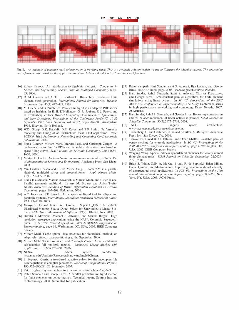
Fig. 6. An example of adaptive mesh refinement on a traveling wave. This is a synthetic solution which we use to illustrate the adaptive octrees. The coarseningand refinement are based on the approximation error between the discretized and the exact function.

[16] Robert Falgout. An introduction to algebraic multigrid. Computing inScience and Engineering, Special issue on Multigrid Computing, 8:24–33, 2006.

[17] D. M. Greaves and A. G. L. Borthwick. Hierarchical tree-based finiteelement mesh generation. International Journal for Numerical Methodsin Engineering, 45(4):447–471, 1999.

[18] M. Griebel and G. Zumbusch. Parallel multigrid in an adaptive PDE solverbased on hashing. In E. H. D’Hollander, G. R. Joubert, F. J. Peters, andU. Trottenberg, editors, Parallel Computing: Fundamentals, Applicationsand New Directions, Proceedings of the Conference ParCo’97, 19-22September 1997, Bonn, Germany, volume 12, pages 589–600, Amsterdam,1998. Elsevier, North-Holland.

[19] W.D. Gropp, D.K. Kaushik, D.E. Keyes, and B.F. Smith. Performancemodeling and tuning of an unstructured mesh CFD application. Proc.SC2000: High Performance Networking and Computing Conf.(electronicpublication), 2000.

[20] Frank Gunther, Miriam Mehl, Markus Pogl, and Christoph Zenger. Acache-aware algorithm for PDEs on hierarchical data structures based onspace-filling curves. SIAM Journal on Scientific Computing, 28(5):1634–1650, 2006.

[21] Morton E. Gurtin. An introduction to continuum mechanics, volume 158of Mathematics in Science and Engineering. Academic Press, San Diego,2003.

[22] Van Emden Henson and Ulrike Meier Yang. BoomerAMG: a parallelalgebraic multigrid solver and preconditioner. Appl. Numer. Math.,41(1):155–177, 2002.

[23] Frank H ulsemann, Markus Kowarschik, Marcus Mohr, and Ulrich R ude.Parallel geometric multigrid. In Are M. Bruaset and Aslka Tveito,editors, Numerical Solution of Partial Differential Equations on ParallelComputers, pages 165–208. Birk auser, 2006.

[24] A.C. Jones and P.K. Jimack. An adaptive multigrid tool for elliptic andparabolic systems. International Journal for Numerical Methods in Fluids,47:1123–1128, 2005.

[25] Xiaoye S. Li and James W. Demmel. SuperLU DIST: A ScalableDistributed-Memory Sparse Direct Solver for Unsymmetric Linear Sys-tems. ACM Trans. Mathematical Software, 29(2):110–140, June 2003.

[26] Dimitri J. Mavriplis, Michael J. Aftosmis, and Marsha Berger. Highresolution aerospace applications using the NASA Columbia Supercom-puter. In SC ’05: Proceedings of the 2005 ACM/IEEE conference onSupercomputing, page 61, Washington, DC, USA, 2005. IEEE ComputerSociety.

[27] Miriam Mehl. Cache-optimal data-structures for hierarchical methods onadaptively refined space-partitioning grids, September 2006.

[28] Miriam Mehl, Tobias Weinzierl, and Christoph Zenger. A cache-obliviousself-adaptive full multigrid method. Numerical Linear Algebra withApplications, 13(2-3):275–291, 2006.

[29] NCSA. Abe’s system architecture.ncsa.uiuc.edu/UserInfo/Resources/Hardware/Intel64Cluster.

[30] S. Popinet. Gerris: a tree-based adaptive solver for the incompressibleEuler equations in complex geometries. Journal of Computational Physics,190:572–600(29), 20 September 2003.

[31] PSC. Bigben’s system architecture. www.psc.edu/machines/cray/xt3.

[32] Rahul Sampath and George Biros. A parallel geometric multigrid methodfor finite elements on octree meshes. Technical report, Georgia Instituteof Technology, 2008. Submitted for publication.

[33] Rahul Sampath, Hari Sundar, Santi S. Adavani, Ilya Lashuk, and GeorgeBiros. Dendro home page, 2008. www.cc.gatech.edu/csela/dendro.

[34] Hari Sundar, Rahul Sampath, Santi S. Adavani, Christos Davatzikos,and George Biros. Low-constant parallel algorithms for finite elementsimulations using linear octrees. In SC ’07: Proceedings of the 2007ACM/IEEE conference on Supercomputing, The SCxy Conference seriesin high performance networking and computing, Reno, Nevada, 2007.ACM/IEEE.

[35] Hari Sundar, Rahul S. Sampath, and George Biros. Bottom-up constructionand 2:1 balance refinement of linear octrees in parallel. SIAM Journal onScientific Computing, 30(5):2675–2708, 2008.

[36] TACC. Ranger’s system architecture.www.tacc.utexas.edu/resources/hpcsystems.

[37] Trottenberg, U. and Oosterlee, C. W. and Schuller, A. Multigrid. AcademicPress Inc., San Diego, CA, 2001.

[38] Tiankai Tu, David R. O’Hallaron, and Omar Ghattas. Scalable paralleloctree meshing for terascale applications. In SC ’05: Proceedings of the2005 ACM/IEEE conference on Supercomputing, page 4, Washington, DC,USA, 2005. IEEE Computer Society.

[39] Weigang Wang. Special bilinear quadrilateral elements for locally refinedfinite element grids. SIAM Journal on Scientific Computing, 22:2029–2050, 2001.

[40] Brian S. White, Sally A. McKee, Bronis R. de Supinski, Brian Miller,Daniel Quinlan, and Martin Schulz. Improving the computational intensityof unstructured mesh applications. In ICS ’05: Proceedings of the 19thannual international conference on Supercomputing, pages 341–350, NewYork, NY, USA, 2005. ACM Press.

12