TECH

Friedr

Den

neur

Hong

VollstänErlangu

Doctor

genehm

Vorsitz

Prüfer d

1. Univ.

2. Prof.

Die DissMünche

HNISCHE

rich-Sch

dritic o

rons in

bo Jia

ndiger Abdrung des aka

of Philoso

migten Disse

ender: Univ

der Dissert

-Prof. Dr. A

Dr. Bert Sa

sertation wuen eingereic

UNIVER

iedel Ins

organi

n vivo

uck der vonademischen

ophy (Ph.D.

ertation.

v.-Prof. Dr.

tation:

Arthur Konne

akmann

urde am 09cht und durc

RSITÄT M

stitut für

ization

n der Fakult Grades ein

.)

Thomas M

erth

.08.2011 bech die Faku

MÜNCHE

Neurowi

n of se

tät für Mediznes

isgeld

ei der Fakuultät für Med

EN

issensch

nsory

zin der Tec

ltät für Meddizin am 02

haften

inputs

hnischen U

izin der Tec.11.2011 an

s in co

Universität M

chnischen Ungenommen

rtical

München zu

Universität n.

r

Abstract

Mammalian cortical neurons compute sensory information that arrives through numerous

synaptic inputs located on their dendrites. These inputs are essential for various computational

functions of neurons. However, it has long been a major challenge to identify sensory

stimulation‐activated individual synaptic inputs in cortical neurons in vivo. I have implemented

and applied the combined method of two‐photon calcium imaging and whole‐cell patch‐clamp

recording to study layer 2/3 cortical neurons in mouse visual cortex and identified orientation‐

specific dendritic input sites for the first time. When the neuron was slightly hyperpolarized just

below action potential firing threshold, multiple dendritic calcium hotspots could be observed

upon visual stimulation of a given orientation. These hotspots were spatially restricted to small

dendritic domains and sensitive to NMDA receptor antagonist, thus representing sensory

evoked synaptic input sites. An important finding was that input sites with different orientation

preference were intermingled throughout the dendritic tree. Furthermore, all neurons received

multiple inputs of different orientation preferences, regardless whether the action potential

output had a specific preference or not.

Overall, I have established the combined method of in vivo whole‐cell recording and

two‐photon calcium imaging and implemented efficient data analysis algorithms for studying

sensory evoked dendritic inputs in mammalian cortical neurons in vivo. Articles involving these

major findings have been published or accepted by peer‐reviewed journals. As a result, this

dissertation is composed of the accumulation of related articles together with brief summary

and specification of personal contributions.

Table of Contents

Personal considerations 1‐3

1 Overview: Dendritic mapping of sensory inputs in vivo 4‐7

2 Dendritic organization of sensory input to cortical neurons in vivo

Background 8

Reprint by Nature 2010 Apr 29;464(7293):1307‐12. 9‐21

3 In vivo two‐photon imaging of sensory‐evoked dendritic calcium

signals in cortical neurons

Background 22

Reprint by Nat Protoc. 2011 Jan;6(1):28‐35. 23‐30

4 Dendritic coding of multiple sensory inputs in single cortical

neurons in vivo

Background 31

Original manuscript accepted by PNAS 32‐63

5 Calcium imaging in the living brain: prospects for molecular

medicine

Background 64

Reprint by Trends Mol. Med. 2008 Sep;14(9):389‐99. 65‐75

6 Other activities: Custom built video‐rate two‐photon microscopy

setup 76‐79

7 Summary and specification of contributions to published articles

80‐82

Acknowledgements 83

Personal considerations

As one of the 80s’ generation, I have always been fascinated by the intelligent robots that

appeared in Hollywood movies like Star Wars, Terminator, etc. But in reality, would it possible

to build such machines?

In fact the key issue is not how to build a self‐moving robot, but rather, what is

intelligence? If we (=humans) acknowledge that the creation of steam engines was based on the

knowledge of physics, we can as well say that the creation of intelligent robots should be based

on the knowledge of brain. Apparently our knowledge of physics is quite advanced at the

moment, and in fact has greatly helped the understanding of brain. However, our knowledge of

brain, fairly speaking, is still quite modest. In contrast to the systematic theories of physics,

theories of neuroscience, although numerous, were rather like scattered stars in the sky. The

main problem was the fact that each measurement of brain could only acquire very little

information from all that a brain holds, typically, recording from 1 to 103 neurons out of total

106 to 1012 in animals that are considered to be “intelligent”.

However, thanks to the development of electronic computers, we can simulate more

number of neurons than that we could record from a real brain. But have that created

intelligence? Unfortunately, not yet. Perhaps what matters more are not the numbers, but

something else, for example, rules. What rules then? Conventional intuition of rules, as well as

classical physics, tells us that everything should be exactly predicted by the rules, well, not really

like living animals would normally behave.

No worries, physics also tells us that even simple and fixed rules can generate complex

and unpredictable behaviors, i.e., the “chaos”. But do not yet draw equality between

“intelligence” and “chaos”, since we have not known what the specific underlying rules are.

What we can do is to try our best to get as much information as possible from measurements of

brain, and then think on mathematical rules that would describe them properly. Such rules must

be consistent with each other, and more importantly, also consistent with existing rules of

physics. Only by doing so would allow us to “create” intelligence ab initio on a machine instead

of “simulate” intelligence with a machine. The difference is that, if we leave that machine alone,

Page 1 / 83

whether it remains intelligent or not.

So, it is clear that we must now focus on measuring the brain. What should we measure

then, weight, color, or shape? Apparently we know that these properties do not have much to

do with intelligence. Electricity is the answer, or at least, the belief of most neuroscientists.

Electricity can be measured from objects at various scales depending on where and how the

electrodes are placed: the whole brain, or a small volume of brain, a bunch of cells, a single cell,

or a part of a cell.

Actually one of the most basic and famous measurements were just about a few protein

molecules which could let ions flow through membranes of neurons. Unfortunately, such

measurements cannot be performed in a living brain because the molecules to be measured

must be isolated from the rest of their host cell and the brain. Nevertheless, the results of these

measurements formed the ground level rules that support the other rules which would be

concluded from measurements of larger objects.

Therefore we go one level up, to the parts of a cell. Is it possible to simultaneously

measure different parts of a cell in a living animal’s brain without isolating them from the brain?

As I present in this dissertation, yes. But I used a different measurement method, that the fine

processes of the cell were measured by fluorescence indicators for a fraction of Ca2+ ions.

However, thanks to the ground level rules we were able to use these fluorescence signals to

represent specific electrical activities.

One may ask, why not measure at the other scales? The straightforward answer is that,

other people had done many measurements at those scales, while my advisor needed to get me

something new to do so that I could get food in the future if I would still work on neuroscience.

However, what I have begun to understand later on after my measurements was that,

measuring parts of a cell is not only measuring for this cell, but simultaneously measuring some

other cells who connects to this cell at the measured locations.

Connectivity, especially long‐range connectivity is one of the most important features of

brain. As a contrast, cells in other organs interact mostly with their nearest neighbours. The

enormous amount of interconnections in a brain made it almost impossible to capture all of

Page 2 / 83

them, but we now have a simple scenario: one node of the network with a fraction of

connections to that node. We could study how this single node of network represents the

external physical world and/or other parts of the neuronal network that are related to it, which

was my little contribution to the entire human knowledge of brain.

For most time of my dissertation research, I built measurement machines, measured a

few neurons in mice brains and reported the results by electronic computers. Thanks to the

new rules of the graduate school, I would not spend much time in re‐organizing my old

knowledge that had already been published in peer‐reviewed journals. I will organize the entire

papers (permissions have been acquired) in individual chapters, provide brief introduction to

the background of each study, and then give general overview and summary chapters. The time

being saved in this way can be then used for further experimental works on the neuronal

organization of brain as well as thinking on a physical theory of describing brain function, which

perhaps can eventually lead to realization of the dream of creating intelligent machines.

Hongbo Jia

22/07/2011 at Munich

Page 3 / 83

1 Overview: Dendritic mapping of sensory inputs in vivo

As a canonical viewpoint of neuroscience, brain function relies on the network of synaptically

interconnected neurons. Neurons of the mammalian brain communicate with each other mostly

though chemical synapses. Excitatory synapses using glutamate as a transmitter form many of

their contacts with fine dendritic protrusions, the so‐called spines (1). In the cortex, for example,

single pyramidal neurons receive thousands of synaptic inputs on such spines (2). An

understanding of the dendritic organization of the synaptic inputs is important because of the

great potential of signal integration and computation (3, 4). In recent years there had been

substantial progress in our understanding of the local connectivity in selected brain regions (5‐7).

However, despite many years of detailed anatomical studies (8) and more recent efforts of

revealing the brain’s connectome (9), the functional organization of the synaptic connectivity in

vivo, in relation to defined sensory stimuli, is still largely unknown. One important question, for

example, is how are sensory stimulation activated dendritic input sites organized in single

cortical neurons in vivo (10).

One common way of studying synaptic function in dendrites consists in the analysis of

postsynaptic signals, for example the calcium transients induced by synaptic activity (11). Such

studies under in vitro conditions were usually performed by imaging with fluorescent calcium

indicators near the site of focal extracellular synaptic stimulation (12). However, for mammalian

cortical neurons, the anatomical knowledge acquired from brain slices has not yet been

sufficient to determine a priori which input sites would actually be activated by given sensory

stimulation under in vivo condition. Therefore, in order to be able to identify the stimulation

activated synaptic calcium signaling sites in vivo, one challenge was to simultaneously image as

many dendrites as possible while having sufficient temporal resolution to resolve calcium

transients. Yet another difficulty came after that sensory stimuli are likely to trigger action

potential firing. Action potentials are back‐propagated to dendrites in widespread manner (13,

14), interact with synaptic activity and result in compound calcium signals (15). Although it was

possible to correlate the compound dendritic signals with sensory stimuli in lower vertebrates

(16), such analysis had not yet been unambiguously established for mammalian cortical neurons

in vivo. In contrast, for some specific type of non‐spiking neurons (17‐19) it was feasible to

Page 4 / 83

directly map dendritic calcium signals to specific sensory stimuli. Therefore, the prevention of

action potential firing is important for the revelation of sensory activated synaptic calcium

signaling sites in cortical neurons in vivo.

To overcome these challenges for identifying sensory stimuli activated dendritic input

sites in cortical neurons, I have employed the combined method of whole‐cell recording and

rapid full‐frame two‐photon calcium imaging. Whole‐cell recording could provide efficient

hyperpolarization to prevent action potential firing, while rapid full‐frame scanning allowed

simultaneous imaging of multiple dendrites in the focal plane. Furthermore, significant

improvements in experimental procedures (20) enabled long‐lasting recording of sensory

evoked local dendritic calcium signals in mammalian cortical neurons in vivo. With these

advantages, this method had enabled the mapping of visual stimulation evoked dendritic input

sites in layer 2/3 neurons of mouse primary visual cortex (21).

Furthermore, the combined method of in vivo whole‐cell recording and two‐photon

calcium imaging has been applied in subsequent experimental studies in the auditory cortex and

barrel cortex (22, 23). The basic numerical analysis tools which were developed during the first

study were also applied in these studies. Specifically, for the dendritic mapping of individual

whiskers in barrel cortex (chapter 4), an automatic pattern recognition algorithm was employed

that successfully distinguished the dendritic activation patterns of different whiskers for each

single trial at high accuracy. In combination, a theoretical model was also devised to verify the

analysis on experimental data.

In the next chapters, the published research articles for which I had significant

contributions will be presented with brief background introductions respectively. Besides, since

calcium imaging alone is a widely applied method to study brain function and disease, a

literature review on calcium imaging will be also attached. Additionally, the technical features of

the two‐photon microscopy setup on which the experiments had been performed will be

demonstrated. Finally, I will specify my personal contributions in the related published/accepted

articles.

Page 5 / 83

References

1. Purves, D., Augustine, G. J., Fitzpatrick, D., Hall, W. C., LaMantia, A.‐S., McNamara, J. O.,

& White, L. E. (2008) Neuroscience (Sinauer Associates).

2. Ballesteros‐Yanez, I., Benavides‐Piccione, R., Elston, G. N., Yuste, R., & DeFelipe, J. (2006)

Density and morphology of dendritic spines in mouse neocortex. Neuroscience 138, 403‐

409.

3. Silver, R. A. (2010) Neuronal arithmetic. Nature reviews 11, 474‐489.

4. Branco, T. & Hausser, M. (2010) The single dendritic branch as a fundamental functional

unit in the nervous system. Current opinion in neurobiology 20, 494‐502.

5. Katz, L. C. & Dalva, M. B. (1994) Scanning laser photostimulation: a new approach for

analyzing brain circuits. Journal of neuroscience methods 54, 205‐218.

6. Nikolenko, V., Poskanzer, K. E., & Yuste, R. (2007) Two‐photon photostimulation and

imaging of neural circuits. Nature methods 4, 943‐950.

7. Petreanu, L., Mao, T., Sternson, S. M., & Svoboda, K. (2009) The subcellular organization

of neocortical excitatory connections. Nature 457, 1142‐1145.

8. Cajal, S. R. y. (1995) Histology of the Nervous System of Man and Vertebrates (Oxford

University Press).

9. Lichtman, J. W., Livet, J., & Sanes, J. R. (2008) A technicolour approach to the

connectome. Nature reviews 9, 417‐422.

10. Priebe, N. J. & Ferster, D. (2010) Neuroscience: Each synapse to its own. Nature 464,

1290‐1291.

11. Sabatini, B. L., Maravall, M., & Svoboda, K. (2001) Ca(2+) signaling in dendritic spines.

Current opinion in neurobiology 11, 349‐356.

12. Yuste, R. & Denk, W. (1995) Dendritic spines as basic functional units of neuronal

integration. Nature 375, 682‐684.

13. Helmchen, F., Svoboda, K., Denk, W., & Tank, D. W. (1999) In vivo dendritic calcium

dynamics in deep‐layer cortical pyramidal neurons. Nature neuroscience 2, 989‐996.

14. Svoboda, K., Helmchen, F., Denk, W., & Tank, D. W. (1999) Spread of dendritic excitation

in layer 2/3 pyramidal neurons in rat barrel cortex in vivo. Nature neuroscience 2, 65‐73.

Page 6 / 83

15. Waters, J., Larkum, M., Sakmann, B., & Helmchen, F. (2003) Supralinear Ca2+ influx into

dendritic tufts of layer 2/3 neocortical pyramidal neurons in vitro and in vivo. J Neurosci

23, 8558‐8567.

16. Bollmann, J. H. & Engert, F. (2009) Subcellular topography of visually driven dendritic

activity in the vertebrate visual system. Neuron 61, 895‐905.

17. Euler, T., Detwiler, P. B., & Denk, W. (2002) Directionally selective calcium signals in

dendrites of starburst amacrine cells. Nature 418, 845‐852.

18. Briggman, K. L., Helmstaedter, M., & Denk, W. (2011) Wiring specificity in the direction‐

selectivity circuit of the retina. Nature 471, 183‐188.

19. Elyada, Y. M., Haag, J., & Borst, A. (2009) Different receptive fields in axons and

dendrites underlie robust coding in motion‐sensitive neurons. Nature neuroscience 12,

327‐332.

20. Jia, H., Rochefort, N. L., Chen, X., & Konnerth, A. (2011) In vivo two‐photon imaging of

sensory‐evoked dendritic calcium signals in cortical neurons. Nature protocols 6, 28‐35.

21. Jia, H., Rochefort, N. L., Chen, X., & Konnerth, A. (2010) Dendritic organization of sensory

input to cortical neurons in vivo. Nature 464, 1307‐1312.

22. Chen, X., Leischner, U., Rochefort, N. L., Nelken, I., & Konnerth, A. (2011) Functional

mapping of single spines in cortical neurons in vivo. Nature.

23. Varga, Z., Jia, H., Sakmann, B., & Konnerth, A. (2011) Dendritic coding of multiple sensory

inputs in single cortical neurons in vivo. Proc Natl Acad Sci U S A (accepted).

Page 7 / 83

2 Dendritic organization of sensory input to cortical neurons in vivo

Background

This article included the major results of my thesis work, and was the first report of in vivo

dendritic input mapping in cortical neurons. Before having achieved these results, many

preliminary experiments had been performed with various methods. One series of those

experiments, for example, involved two‐photon imaging of single layer 2/3 visual cortical

neuron after electroporation of calcium dye. In both basal and oblique dendrites, the dominant

type of signals found were the widespread global calcium transients that were either

spontaneous or visually evoked. Loose cell‐attach recordings on the electroporated neuron

showed that these widespread dendritic calcium signals were correlated with action potential

firings. Thus, these widespread calcium signals on basal and oblique dendrites were likely to be

induced by back‐propagation of action potentials (bAPs), similar to previously reported (as ref

#7, 9 in the original paper) recordings on the apical trunk dendrites. Therefore, whole‐cell

recording was employed, with the idea to use depolarizing current pulse to induce action

potentials and thus testing their causality in the global dendritic calcium signals. However, it

turned out to be not easy to precisely induce a fixed number of action potentials due to large

fluctuations of synaptic current of the neuron itself. Then the strategy was changed to the

prevention of action potential firing, which was easily achieved by hyperpolarizing the neuron

until sufficient level. When the widespread bAPs‐related dendritic calcium signals were

abolished under this condition, the sensory input related local dendritic calcium signals could be

detected. With this key rendered by the combination of whole‐cell recording and two‐photon

calcium imaging, the gate to the mapping of sensory input to cortical neurons in vivo was

eventually opened.

Page 8 / 83

ARTICLES

Dendritic organization of sensory input tocortical neurons in vivoHongbo Jia1*, Nathalie L. Rochefort1*, Xiaowei Chen1 & Arthur Konnerth1

In sensory cortex regions, neurons are tuned to specific stimulus features. For example, in the visual cortex, many neuronsfire predominantly in response to moving objects of a preferred orientation. However, the characteristics of the synapticinput that cortical neurons receive to generate their output firing pattern remain unclear. Here we report a novel approach forthe visualization and functional mapping of sensory inputs to the dendrites of cortical neurons in vivo. By combininghigh-speed two-photon imaging with electrophysiological recordings, we identify local subthreshold calcium signals thatcorrespond to orientation-specific synaptic inputs. We find that even inputs that share the same orientation preference arewidely distributed throughout the dendritic tree. At the same time, inputs of different orientation preference areinterspersed, so that adjacent dendritic segments are tuned to distinct orientations. Thus, orientation-tuned neurons cancompute their characteristic firing pattern by integrating spatially distributed synaptic inputs coding for multiple stimulusorientations.

A growing amount of evidence indicates that information processingin the brain involves the computation of electrical and chemicalsignals in neuronal dendrites (for a review, see ref. 1). One of themost effective ways for the analysis of these dendritic signals relies onthe imaging of the dynamics of intracellular Ca21 concentration(reviewed in ref. 2). Thus, synaptic input-related dendritic Ca21

transients have been identified and studied in detail in vitro3–6, whilein vivo work has explored action-potential-related dendritic Ca21

signals7–9. However, nothing is known about the nature of subthres-hold sensory evoked input signals in the dendrites of mammaliancortical neurons. A detailed knowledge of sensory input signalswould represent an important step forward in the understandingof dendritic computation1,10–13. An intriguing open question iswhether sensory inputs with similar features are clustered on thesame dendrite of a neuron or dispersed throughout the dendritictree. Clustered inputs are capable of generating dendritic spikes(reviewed in ref. 11) and may form neuronal computational subunitsin vivo, as they do under certain experimental conditions in vitro14.Alternatively, sensory inputs that are not clustered, but widely dis-tributed, may underlie different rules of integration and formation ofneuronal output signals—like, for example, the linear summation ofexcitatory inputs15.

Visually evoked supra- and subthreshold activity

For the functional analysis of spiny dendrites in vivo by means of two-photon calcium imaging, we selected as an experimental model neu-rons in layer 2/3 of the mouse primary visual cortex (Fig. 1a–c). Thesomata of the neurons were located approximately between 140 and200mm below the cortical surface. Their dendritic trees had a char-acteristic pattern, consisting of numerous basal and oblique dendritesbut no pronounced apical trunk16–18 (Fig. 1a). As in many other mam-malian species19–21, layer 2/3 neurons of the mouse primary visualcortex respond selectively to drifting gratings or bars with actionpotential firing22–24. By performing whole-cell recordings involvingthe ‘shadow-patching’ approach25, we found that stimulation withdrifting gratings shifted the membrane potential to the ‘up-state’26

for the entire duration of the stimulus. An increased probability ofup-states during drifting grating stimulation was previously observedin the cat visual cortex27. The neuron illustrated in Fig. 1d fired actionpotentials preferentially during the presentation of specificallyoriented drifting gratings and was identified as a ‘highly-tuned’ neu-ron (Fig. 1e left) on the basis of its orientation selectivity index (OSI),which was higher than 0.5 (Methods). In our recordings, 6 out of 17neurons were highly tuned for a preferred orientation (Fig. 1f left),6/17 neurons were poorly tuned, while the rest of 5/17 neurons did notrespond reliably to visual stimulation. For a better assessment of thestimulus-evoked subthreshold depolarization in highly tuned neu-rons, we hyperpolarized them to subthreshold membrane potentials.In the example shown in Fig. 1d, the neuron was hyperpolarized fromits resting level of 264 mV to 270 mV. In contrast to the highly tunedaction potential pattern (Fig. 1e left), the stimulus-evoked subthres-hold depolarizing responses were broadly tuned in this (Fig. 1e right)as well as in all other highly tuned neurons (Fig. 1f right). Thus, inmouse visual cortex, as in cat visual cortex28,29, the high tuning level ofaction potential firing, the neuronal output signal, contrasts with thelow tuning level of the afferent subthreshold input signals.

These observations prompted us to combine whole-cell recordingswith two-photon calcium imaging to search for dendritic signalsassociated with the afferent activity. We performed high-speedtwo-photon imaging at 30 full frames per second or 60 half framesper second using resonant galvo-scanners30 and, initially, focused onthe dendrites that were visible in the plane of focus containing the cellbody (Fig. 1g). When stimulated with their preferred orientation,neurons responded with action potential firing that was associatedwith global dendritic calcium transients in all imaged dendrites. Inthe neuron illustrated in Fig. 1g, all five visible dendrites displayedcalcium transients that were larger when the neuron fired four actionpotentials (Fig. 1h left) than when it fired two action potentials(Fig. 1h right). The dependence of the calcium transient amplitudeon the number of action potentials and the observation that similarcalcium transients were evoked by direct neuronal depolarizationthrough the recording pipette (Supplementary Fig. 1a–c) indicate

*These authors contributed equally to this work.

1Institute of Neuroscience and Center for Integrated Protein Science, Technical University Munich, Biedersteinerstrasse 29, 80802 Munich, Germany.

Vol 464 | 29 April 2010 | doi:10.1038/nature08947

1307Macmillan Publishers Limited. All rights reserved©2010

Page 9 / 83

that such global dendritic signals are largely due to the activation ofvoltage-gated calcium channels by back-propagating action poten-tials; this has previously been shown for basal dendrites in in vitrorecordings from layer 2/3 neurons31,32. The amplitude of the Ca21

transients at different dendritic sites showed attenuation along agiven dendrite (Supplementary Fig. 1d, e) and variations from trialto trial, but we were unable to obtain unambiguous evidence forsignal peaks that would correspond to specific synaptic inputs, asfound in tectal neurons of the tadpole33. Therefore, we decided tosearch for calcium signals associated with subthreshold synaptic

calcium signalling in conditions in which we actively hyperpolarizedthe neurons.

Subthreshold calcium signals in dendritic hotspots

Figure 2 illustrates the results of an experiment in which a neuron washyperpolarized to 270 mV to prevent action potential firing. In theseconditions, a calcium transient was evoked in a subregion of ‘dend-rite 3’ (Fig. 2a, b) by visual stimulation (drifting grating), but notdetected in the other dendrites or in the soma. To assess the spatialdimensions of such local calcium transients, we analysed experiments

a c

Spike rate

0º45º

90º

135º180º

225º

270º

315º0º

45º

90º

135º180º

225º

270º

315º

Subthreshold depolarization

0º 90º270º 180º

100%

0%0º 90º270º 180º

100%

0%

n=6 neurons

Nor

mal

ized

sp

ike

rate

L1

L2/3

L4

L5

L6

100 µm

n=6 neurons

Nor

mal

ized

sub

thre

shol

dd

epol

ariz

atio

n

20 mV

1 s

Patch pipette(OGB1, Alexa,biocytin)

b

Neuron 2, –173 µm

12

3

45

10 µm

0.2 Δf/f

1 s

20 mV

Primary visual cortex5 µm 20 µm

–64 mV

–70 mV

d

1

2

3

4

5

Soma

4 APs 2 APsVm

e

f

g

h

Orientation Orientation

Figure 1 | Visually evoked action potentials, subthreshold depolarizationsand global dendritic calcium signals. a, Reconstruction of a biocytin-filledlayer 2/3 (L2/3) neuron in mouse primary visual cortex (projection along theantero-posterior axis). Data from the same neuron are presented inb–e. b, Microphotograph of a spiny basal dendrite. c, Projection along thedorso-ventral axis obtained in vivo from 469 sections (step size 0.5 mm) fromAlexa fluorescence. d, Whole-cell current-clamp recordings of responses todrifting gratings of different orientations. Three trials were superimposed.Upper red traces, action potential responses at resting potential (indicatedon the left); lower blue traces, subthreshold responses obtained afterhyperpolarizing the neuron to 270 mV. e, Polar plots of visually evokedresponses, average of eight trials. Red plot, spike rate; blue plot, amplitude ofsubthreshold depolarization. f, Tuning properties of spiking and

subthreshold responses for six orientation-selective neurons, eachnormalized to their preferred orientation (noted as 0u). Error bars, 1s.d.g, h, Two-photon imaging of dendritic calcium signals in basal and obliquedendrites of another layer 2/3 neuron during action potential firing(electrical recording lower red trace) evoked by drifting gratings. g, Averageimage of 100 frames recorded at 173mm below the cortical surface. Yellowdashed lines indicate out-of-focus portions of the dendrites. Green dashedlines indicate the regions of interest (ROIs). h, Ca21-dependent fluorescencechanges (black traces) recorded in the soma and in five dendrites (indicatedby numbers in g) and the corresponding membrane potential (Vm, redtraces) recordings, during two separate trials. Light grey bars indicate thestimulation period with oriented gratings. AP, action potential.

ARTICLES NATURE | Vol 464 | 29 April 2010

1308Macmillan Publishers Limited. All rights reserved©2010

Page 10 / 83

in which long portions of the same dendrite were discernible in theplane of focus of our recordings. In the neuron shown in Fig. 2c, weidentified two dendritic hotspots of visually evoked local calciumtransients. The systematic analysis of segments with a length of3 mm along the dendrite showed that the calcium signal was presentin three neighbouring segments with a clear peak in the middle seg-ment (Fig. 2c, d). Repetitive visual stimulation reliably evoked localdendritic calcium signals (Fig. 2e; mean failure rate 22 6 18%,61 hotspots in 17 neurons). The spatial extent of these dendritichotspots had an average half-width at half-maximum (HWHM) of3.7 6 0.8 mm (n 5 50) (Fig. 2f).

What is the mechanism underlying these calcium signals? First, wenoticed that the NMDA (N-methyl-D-aspartate) receptor antagonistD(2)-2-amino-5-phosphonovaleric acid (AP5) caused a major atte-nuation of the calcium transients, indicating their synaptic origin(Fig. 2g, h). Second, the dimensions of the hotspots were quite similarto the active dendritic shaft segments of pyramidal neurons in vitrodisplaying calcium transients as a result of the spread of calcium fromsingle active spines34,35. In line with this possibility, we also identifiedspines at the hotspot region when constructing post hoc ‘super-average’ images (Fig. 2c bottom). Furthermore, previous record-ings performed in basal dendrites of neocortical neurons in vitro

demonstrated that focally evoked subthreshold excitatory post-synaptic potentials induce calcium transients in dendritic compart-ments of comparable dimensions14. In our recordings, the meanamplitude of hotspot calcium transients (Methods) was Df/f 5 0.25 6 0.07 (n 5 50). This value is comparable to the amplitudesof back-propagating action-potentials-dependent dendritic calciumtransients evoked by the preferred orientation (Df/f 5

0.37 6 0.13, mean number of action potentials 3.1 6 1.1, n 5 50;Supplementary Fig. 1c). Thus, the amplitude and the spatial extentof these visually evoked calcium transients resemble those generatedby individual synaptic inputs, but not those evoked by dendriticNMDA spikes, which produce calcium transients that cover largerdendritic domains and have manifold larger amplitudes31,36,37.

Mapping dendritic distribution of sensory inputs

To determine the spatial distribution of the dendritic hotspotsreflecting sensory inputs, we performed experiments in which weattempted to image as many focal planes as possible in every neuron,requiring 1–2 h of whole-cell recording. In each focal plane, we deter-mined the orientation preference of the local calcium signals by pre-senting drifting gratings (Methods). Figure 3a illustrates anexperiment in which four focal planes were imaged at various depthsunder the cortical surface. A total of 13 hotspots were identified inthis neuron. Figure 3b shows the response from three selected hot-spots (numbered 4, 12 and 7 in Fig. 3a) obtained during presentationof eight directions of drifting gratings. From these averaged calciumtransients (n 5 6 trials), we constructed polar plots for each hotspot(Fig. 3c). A closer inspection of the polar plots revealed the presenceof multiple orientation preferences in this and all other neurons. Thedendritic distribution of the orientation preferences did not appearto follow any strict rule, but seemed to be randomly distributedthroughout the dendritic tree. Another remarkable finding is thatthe calcium transients of most local dendritic hotspots displayed apronounced orientation preference. In order to quantify the tuninglevel, we calculated the OSI for each hotspot and found that themajority of hotspots (72%, n 5 102) were highly tuned for a particu-lar orientation (OSI . 0.5). The average OSI value for all hotspots ofthe neuron shown in Fig. 3 was 0.63. Comparable results wereobtained from 16 additional neurons (mean OSI 5 0.59; n 5 102

1 s

a

g

10 µm

1

2

4

5

Avg. 5 trialsSingle trial

1

2

Soma

3

4

5

–70 mV

20 mV

b

c

(n = 50)HWHM = 3.7 ± 0.8 µm

f

1050–5–10

0.4

0.3

0.2

0.1

0.0

Δf/f

Distance (µm)

0.1 Δf/f

0.1 Δf/f

1 s

Control

AP5

Wash-out

100%

0%

Nor

mal

ized

Δf/f

h

Control AP5

***

Super-average

10 µm

AP5 +Alexa

0 0.4

10 µm

3

d

d1 d2 d3 d4 d5

2 s

0.2 Δf/f

d1 d2 d3 d4 d5

e Consecutive trials (red box)

Figure 2 | Subthreshold local dendritic calcium signals evoked by driftinggrating stimulation. a, Two-photon image used for calcium recordings inb. The image is an average of 100 frames. Five ROIs are indicated by greendashed rectangles. b, Subthreshold Ca21 transients (black traces) andcorresponding depolarization (blue traces) evoked by drifting gratingstimulation. Note the prominent Ca21 signal in dendrite 3. Left traces, singletrials; right traces, average (black trace) of five individual trials (grey traces)from various dendritic sites and soma, as indicated. c, Upper panel, pseudo-colour image of local dendritic Ca21 signals. Ratio of the averages of 30frames before and 30 frames during stimulation. Yellow arrows indicate twosites of local dendritic calcium signals. Lower panel, enlarged view of thedashed box indicated in the upper image, ‘super-average’ obtained from 500frames. d, Calcium recordings from five neighbouring dendritic regions of3 mm length (d1–d5, ROIs shown in c), average of five trials. e, Calciumsignals evoked during five consecutive trials within the ROI indicated by thered dashed line in c. f, Amplitude distribution of calcium signals withindendritic hotspots (n 5 50 hotspots, 17 neurons). Grey dashed lines indicatethe Gaussian fitting to the amplitude distribution of calcium signals withinindividual hotspots. Red line indicates the Gaussian fit to all points. Averagehalf-width at half-maximum (HWHM) with standard deviation (6) isindicated. g, Left, two-photon image of a neuron (average n 5 100 frames)and schematic representation of drug application pipette containing AP5and Alexa-594. The red dashed lines indicate the approximate area of drugapplication. The green dashed box is the ROI for calcium monitoring. Right,Ca21 recordings before, during and after the application of AP5. Averagetrace (black line) of five individual trials (grey lines). h, Amplitude of calciumsignals before and during the application of AP5 obtained from n 5 9 localcalcium signals in four neurons. The amplitude of each Ca21 signal wasnormalized to the mean amplitude of all signals in control condition. Pairedt-test, ***P , 0.0001.

NATURE | Vol 464 | 29 April 2010 ARTICLES

1309Macmillan Publishers Limited. All rights reserved©2010

Page 11 / 83

hotspots). An important finding was that dendritic hotspots werefound in each of the recorded neurons (17/17), regardless of thetuning level of action potential firing and even in the neurons thatwere not reliably firing in response to drifting gratings. This suggeststhat these hotspots represent a general and highly reliable feature oflayer 2/3 neurons of the primary visual cortex.

Hotspots of the same orientation preference in a given neuron werefound widely dispersed over various dendrites. For example, in theneuron shown in Fig. 4a left, we identified six hotspots for the stimu-lus orientation indicated in the figure and, remarkably, each hotspotwas on a different dendritic branch. The analysis of a larger set ofneurons (n 5 8, Fig. 4a right) confirmed this widespread distributionand emphasized the absence of any clustering of inputs on singledendrites. Furthermore, hotspots coding for the same orientationwere found throughout the entire three-dimensional space surround-ing the cell body. A similar wide distribution was observed for all fourorientations tested (Supplementary Fig. 2). The absence of input

clustering became particularly obvious when we analysed the inputsto individual dendritic branches. Figure 4b shows three examples ofdendritic branches with neighbouring hotspots that have differentorientation preferences. In 9/10 dendritic branch segments, localizedbetween two branching points, we encountered two or three hotspotstuned for different orientation preferences. In just one out of these 10cases, neighbouring hotspots coded for the same orientation. Thegraph in Fig. 4c right summarizes these results. The left panel ofFig. 4c shows that all ‘full dendrites’, that is, individual dendritestogether with all their higher order branches, received inputs formultiple orientations. Finally, we compared in 12 neurons the tuninglevels of the firing pattern, representing the output signal, with thetuning levels of local dendritic calcium responses, representingthe synaptic input signals. Experimentally, the orientation preferenceof spike firing in these neurons was determined during the initial25–30 min of whole-cell recording during which the calcium indicatordye was allowed to equilibrate in the dendrites. Then, the neurons

–122 µm

–148 µm

–193 µm

–141 µm

a

10 µm

12

3

13

10

12

9

5 6

8

7

4

b

7

4

0.1 Δf/f

1 s

12

0º

180º135º225º

90º270º

45º315º

0º

180º135º225º

90º270º

45º315º

0º

180º135º225º

90º270º

45º315º

0º

180º135º225º

90º270º

45º315º

0º

180º135º225º

90º270º

45º315º

0º

180º135º225º

90º270º

45º315º

0º

180º135º225º

90º270º

45º315º

0º

180º135º225º

90º270º

45º315º0º

180º135º225º

90º270º

45º315º0º

180º135º225º

90º270º

45º315º

0º

180º135º225º

90º270º

45º315º0º

180º135º225º

90º270º

45º315º0º

180º135º225º

90º270º

45º315º

1

2

3

13 10

9

20 µm

8

5

c

74

6 12

11

11

Figure 3 | Heterogeneity and distribution pattern of orientation-tuneddendritic hotspots. a, Four two-photon images (each an average of n 5 100frames) of a layer 2/3 neuron obtained at different depths under the corticalsurface as indicated. Red dashed boxes indicate hotspots of local dendriticcalcium signalling. b, Local dendritic calcium signals evoked by driftinggratings of different orientations (average of six trials) at three different

dendritic sites indicated in a. c, Location of each hotspot indicated as a reddot on the Z-projection of the reconstructed dendritic tree. Red dashed linespoint to the polar plot obtained for the corresponding local Ca21 signals.The frame (grey dashed line) indicates the area of imaging. The output signalof the neuron was tuned for the vertical orientation.

ARTICLES NATURE | Vol 464 | 29 April 2010

1310Macmillan Publishers Limited. All rights reserved©2010

Page 12 / 83

were hyperpolarized and we determined the orientation preferenceof local dendritic calcium signals. We compared six highly tunedneurons (mean OSI 5 0.79) with six broadly tuned ones (meanOSI 5 0.29) (Fig. 4d right). Unexpectedly, the input signals had verysimilar tuning levels for the two neuronal groups, with mean OSI valuesof 0.60 and 0.59, for highly and broadly tuned firing patterns, respec-tively. This disparity between input and output signals, combined with

the above-mentioned observation that all neurons had input signalscoding for multiple orientations, indicates that the orientation pref-erence of the output signal is the result of a computational processtaking place on the level of individual neurons.

Conclusions

Our results reveal basic insights into the dendritic organization ofsensory inputs to neurons of the visual cortex in vivo. First, we iden-tified discrete dendritic hotspots as synaptic entry sites for specificsensory features. These hotspots represent novel dendritic calcium sig-nals in vivo and were found in all layer 2/3 neurons, irrespective of theiroutput firing pattern. Second, we showed that afferent sensory inputswith the same orientation preference are widely dispersed over thedendritic tree and do not converge on single dendrites, as repeatedlyproposed in recent years (see review in ref. 11 and references therein).Third, we found that even neurons with a highly tuned output signalreceive input signals that are heterogeneous and code for multipleorientations and/or directions. Thus, taken together, our results sup-port a neuronal integration model involving summation of distributedinputs, rather than models that stress the role of convergent inputs tosingle dendrites6,15. However, it is certainly possible that other typesof cortical neurons, especially those with pronounced apical tufts38 orneurons in other species with a columnar organization of the visualcortex17,19–21, have more clustered sensory inputs to the same dendrite,capable of generating large amplitude dendritic spikes6,11. Theapproach introduced in this study opens the way to a detailed analysisof various types of neurons followed by the construction of functionalwiring diagrams of sensory pathways with single input resolutionin vivo.

METHODS SUMMARY

C57BL/6 mice (postnatal day (P)28–P34) were prepared for in vivo two-photon

calcium imaging and whole-cell recordings under isoflurane anaesthesia as

described previously39. Whole-cell patch-clamp recordings of layer 2/3 neurons

of primary visual cortex (monocular region) were performed by ‘shadow-patch-

ing’25. Neurons were dialysed with a pipette solution containing the fluorescent

Ca21 indicator Oregon green BAPTA-1 hexapotassium (OGB-1; 100mM),

Alexa-594 (25mM) and biocytin (2 mg ml21). Basal and oblique dendrites that

appeared on the same focal plane were imaged by high-speed two-photon micro-

scopy involving a resonant galvo-scanner30. Membrane potential changes and

Ca21 signals were simultaneously recorded. The focal plane depth and the

imaged area were chosen to contain as many dendrites as possible. At each focal

plane, we imaged the activity evoked by drifting square wave gratings (0.03 cycles

per degree, 1 Hz, eight directions, standing phase 2 s, drifting phase 1 s).

Transient changes in Ca21 fluorescence (Df/f) were systematically examined

by an adaptive algorithm, which involved small regions of interest (ROIs) of

3 3 4mm, noise filtering and pattern matching. The NMDA receptor antagonist

AP5 (together with Alexa-594) was locally applied by pressure ejection close to

the imaged dendrites. The spread of the ejected solution was monitored by

imaging Alexa fluorescence. The tuning level of local dendritic calcium signals

with regard to the orientation of the drifting grating was quantified by an OSI24.

Received 14 October 2009; accepted 24 February 2010.

1. London, M. & Hausser, M. Dendritic computation. Annu. Rev. Neurosci. 28,503–532 (2005).

2. Bloodgood, B. L. & Sabatini, B. L. Ca21 signaling in dendritic spines. Curr. Opin.Neurobiol. 17, 345–351 (2007).

3. Markram, H. & Sakmann, B. Calcium transients in dendrites of neocorticalneurons evoked by single subthreshold excitatory postsynaptic potentials vialow-voltage-activated calcium channels. Proc. Natl Acad. Sci. USA 91, 5207–5211(1994).

4. Nevian, T. & Sakmann, B. Spine Ca21 signaling in spike-timing-dependentplasticity. J. Neurosci. 26, 11001–11013 (2006).

5. Yuste, R. & Denk, W. Dendritic spines as basic functional units of neuronalintegration. Nature 375, 682–684 (1995).

6. Hausser, M. & Mel, B. Dendrites: bug or feature? Curr. Opin. Neurobiol. 13,372–383 (2003).

7. Helmchen, F., Svoboda, K., Denk, W. & Tank, D. W. In vivo dendritic calciumdynamics in deep-layer cortical pyramidal neurons. Nature Neurosci. 2, 989–996(1999).

8. Murayama, M. et al. Dendritic encoding of sensory stimuli controlled by deepcortical interneurons. Nature 457, 1137–1141 (2009).

a

d Input (dendritic Ca2+ signals) Output (spike rate)

OSImean = 0.60

OSImean = 0.59

50%

25%

0%

OSImean = 0.79(Highly tuned neurons)

0 10.5

b One dendrite, multiple orientations

10 µm

Dendrite 1, –193 µm

Dendrite 2, –147 µm

10 µm

Dendrite 3, –137 µm

10 µm

50%

25%

0%

OSImean = 0.29(Poorly tuned neurons)

0 10.5

Superposition of eight neurons

20 µm

One orientation, multiple dendrites

20%

10%

0%

30%

0 10.5

Nor

mal

ized

pro

por

tion

20%

10%

0%

30%

0 10.5

Nor

mal

ized

pro

por

tion

c100%

0%

Pro

por

tion

Fulldendrite

Branchsegment

Mult. Same Mult. SameOrientation(s)

OSI OSI

Figure 4 | Spatial arrangement of dendritic hotspots and input–outputrelation. a, Distribution of dendritic hotspots (red dots) tuned for theorientation preference indicated in the upper left corner, in the dendritic treeof a neuron (left panel). Right panel, summary of the results obtained for thesame orientation in eight neurons. Cell bodies are indicated by the grey-filleddashed circles (black), dendrites are indicated by dashed red lines (Z-projections reconstructed from stacks). b, Three two-photon images ofdendrites (each an average of n 5 100 frames) at higher magnification withhotspots as indicated. Yellow arrows indicate the preferred orientation oflocal calcium signal in the corresponding hotspot. Note that the hotspots indendrites 2 and 3 as well as the two distal hotspots in dendrite 1 were locatedin branch point-delimited segments. c, Summary graphs. Left panel, theproportion of full dendrites (n 5 12) with hotspots coding for multipleorientations versus those with just one and the same orientation ($3hotspots per full dendrite). Right panel, the proportion of branch segments(between two branching points) with hotspots coding for multipleorientations versus those with the same orientation ($2 hotspots perbranch, n 5 10). d, Input–output relations in highly tuned (upper) andpoorly tuned (lower) neurons. The red and blue histograms showorientation selectivity indices (OSIs as indicated) for the input (Ca21 signalsin dendritic hotspots) and the output (spiking rate) of highly and poorlytuned neurons (n 5 6 for each group), respectively.

NATURE | Vol 464 | 29 April 2010 ARTICLES

1311Macmillan Publishers Limited. All rights reserved©2010

Page 13 / 83

9. Svoboda, K., Denk, W., Kleinfeld, D. & Tank, D. W. In vivo dendritic calciumdynamics in neocortical pyramidal neurons. Nature 385, 161–165 (1997).

10. Johnston, D. & Narayanan, R. Active dendrites: colorful wings of the mysteriousbutterflies. Trends Neurosci. 31, 309–316 (2008).

11. Larkum, M. E. & Nevian, T. Synaptic clustering by dendritic signallingmechanisms. Curr. Opin. Neurobiol. 18, 321–331 (2008).

12. Ohki, K. & Reid, R. C. Specificity and randomness in the visual cortex. Curr. Opin.Neurobiol. 17, 401–407 (2007).

13. Magee, J. C. Dendritic integration of excitatory synaptic input. Nature Rev.Neurosci. 1, 181–190 (2000).

14. Polsky, A., Mel, B. W. & Schiller, J. Computational subunits in thin dendrites ofpyramidal cells. Nature Neurosci. 7, 621–627 (2004).

15. Cash, S. & Yuste, R. Linear summation of excitatory inputs by CA1 pyramidalneurons. Neuron 22, 383–394 (1999).

16. Bannister, A. P. Inter- and intra-laminar connections of pyramidal cells in theneocortex. Neurosci. Res. 53, 95–103 (2005).

17. Hirsch, J. A. & Martinez, L. M. Laminar processing in the visual cortical column.Curr. Opin. Neurobiol. 16, 377–384 (2006).

18. Svoboda, K., Helmchen, F., Denk, W. & Tank, D. W. Spread of dendritic excitationin layer 2/3 pyramidal neurons in rat barrel cortex in vivo. Nature Neurosci. 2,65–73 (1999).

19. Hubel, D. H. & Wiesel, T. N. Receptive fields, binocular interaction and functionalarchitecture in the cat’s visual cortex. J. Physiol. (Lond.) 160, 106–154 (1962).

20. Hubel, D. H. & Wiesel, T. N. Receptive fields and functional architecture ofmonkey striate cortex. J. Physiol. (Lond.) 195, 215–243 (1968).

21. White, L. E. & Fitzpatrick, D. Vision and cortical map development. Neuron 56,327–338 (2007).

22. Drager, U. C. Receptive fields of single cells and topography in mouse visualcortex. J. Comp. Neurol. 160, 269–290 (1975).

23. Metin, C., Godement, P. & Imbert, M. The primary visual cortex in the mouse:receptive field properties and functional organization. Exp. Brain Res. 69, 594–612(1988).

24. Niell, C. M. & Stryker, M. P. Highly selective receptive fields in mouse visualcortex. J. Neurosci. 28, 7520–7536 (2008).

25. Kitamura, K., Judkewitz, B., Kano, M., Denk, W. & Hausser, M. Targeted patch-clamp recordings and single-cell electroporation of unlabeled neurons in vivo.Nature Methods 5, 61–67 (2008).

26. Kerr, J. N., Greenberg, D. & Helmchen, F. Imaging input and output of neocorticalnetworks in vivo. Proc. Natl Acad. Sci. USA 102, 14063–14068 (2005).

27. Anderson, J., Lampl, I., Reichova, I., Carandini, M. & Ferster, D. Stimulusdependence of two-state fluctuations of membrane potential in cat visual cortex.Nature Neurosci. 3, 617–621 (2000).

28. Carandini, M. & Ferster, D. Membrane potential and firing rate in cat primaryvisual cortex. J. Neurosci. 20, 470–484 (2000).

29. Bringuier, V., Chavane, F., Glaeser, L. & Fregnac, Y. Horizontal propagation ofvisual activity in the synaptic integration field of area 17 neurons. Science 283,695–699 (1999).

30. Rochefort, N. L. et al. Sparsification of neuronal activity in the visual cortex at eye-opening. Proc. Natl Acad. Sci. USA 106, 15049–15054 (2009).

31. Gordon, U., Polsky, A. & Schiller, J. Plasticity compartments in basal dendrites ofneocortical pyramidal neurons. J. Neurosci. 26, 12717–12726 (2006).

32. Koester, H. J. & Sakmann, B. Calcium dynamics associated with action potentialsin single nerve terminals of pyramidal cells in layer 2/3 of the young rat neocortex.J. Physiol. (Lond.) 529, 625–646 (2000).

33. Bollmann, J. H. & Engert, F. Subcellular topography of visually driven dendriticactivity in the vertebrate visual system. Neuron 61, 895–905 (2009).

34. Kovalchuk, Y., Eilers, J., Lisman, J. & Konnerth, A. NMDA receptor-mediatedsubthreshold Ca21 signals in spines of hippocampal neurons. J. Neurosci. 20,1791–1799 (2000).

35. Noguchi, J., Matsuzaki, M., Ellis-Davies, G. C. & Kasai, H. Spine-neck geometrydetermines NMDA receptor-dependent Ca21 signaling in dendrites. Neuron 46,609–622 (2005).

36. Holthoff, K., Kovalchuk, Y., Yuste, R. & Konnerth, A. Single-shock LTD by localdendritic spikes in pyramidal neurons of mouse visual cortex. J. Physiol. (Lond.)560, 27–36 (2004).

37. Major, G., Polsky, A., Denk, W., Schiller, J. & Tank, D. W. Spatiotemporally gradedNMDA spike/plateau potentials in basal dendrites of neocortical pyramidalneurons. J. Neurophysiol. 99, 2584–2601 (2008).

38. Larkum, M. E., Nevian, T., Sandler, M., Polsky, A. & Schiller, J. Synaptic integrationin tuft dendrites of layer 5 pyramidal neurons: a new unifying principle. Science325, 756–760 (2009).

39. Stosiek, C., Garaschuk, O., Holthoff, K. & Konnerth, A. In vivo two-photon calciumimaging of neuronal networks. Proc. Natl Acad. Sci. USA 100, 7319–7324 (2003).

Supplementary Information is linked to the online version of the paper atwww.nature.com/nature.

Acknowledgements We are grateful to B. Sakmann for discussions and toY. Kovalchuk for help in the initial experiments. This work was supported by grantsfrom the DFG (to A.K.) and the Friedrich Schiedel Foundation. A.K. is a Carl vonLinde Senior Fellow of the Institute for Advanced Study of the TUM. H.J., N.L.R. andX.C. were supported by the DFG (IRTG 1373).

Author Contributions H.J., N.L.R. and X.C. carried out the experiments. H.J., N.L.R.and A.K. performed the analysis. A.K. designed the study and wrote the manuscriptwith the help of all authors.

Author Information Reprints and permissions information is available atwww.nature.com/reprints. The authors declare no competing financial interests.Correspondence and requests for materials should be addressed to A.K.(arthur.konnerth@lrz.tum.de).

ARTICLES NATURE | Vol 464 | 29 April 2010

1312Macmillan Publishers Limited. All rights reserved©2010

Page 14 / 83

SUPPLEMENTARY INFORMATION

1www.nature.com/nature

doi: 10.1038/nature08947

Supplementary Methods

Animals and surgery

All experimental procedures were performed in accordance with institutional animal welfare

guidelines and were approved by the government of Bavaria, Germany. A total of 18 BL/6

mice (P28-P34) were prepared for in vivo experiments, as described previously39. Briefly, the

mice were placed onto a warming plate (38°C) and anaesthetized by inhalation of 1.5%

isoflurane (Curamed, Karlsruhe, Germany) in pure O2. After removing the skin, a custom-

made recording chamber40 was then glued to the skull with cyanoacrylic glue (UHU, Buhl-

Baden, Germany). The mouse was then transferred into the set-up, placed onto a warming

plate (38° C) and continuously supplied with 0.8% isoflurane in pure O2 (breathing rate 110-

130 breaths per minute). A small craniotomy (~0.8×0.6 mm) was performed above the

monocular region of primary visual cortex using a thin (30G) injection needle. The exposed

region was subsequently covered by 2% agar (~1 mm thick) to reduce vibrations of brain

tissue. The recording chamber was perfused with warm (37° C) extracellular perfusion saline

containing (in mM): 125 NaCl, 4.5 KCl, 26 NaHCO3, 1.25 NaH2PO4, 2 CaCl2, 1 MgCl2, 20

glucose, pH 7.4, when bubbled with 95% O2 and 5% CO2. Eye cream (Bepanthen, Bayer,

Germany) was applied on both eyes to prevent dehydration during surgery. After surgery,

the anaesthesia level was decreased to 0.8% isoflurane for recordings (breathing rate 110-

130 breaths per minute).

Electrophysiology and drug application

The position of the primary visual cortex was located according to brain atlas coordinates

(Bregma -3.5 to -4.5 mm, 2 to 2.5 mm lateral to the midline41). In all experiments the correct

location of the recorded neurons was confirmed in vivo by their responses to visual stimuli

and post-hoc by imaging of the stained brain area. In vivo whole-cell patch-clamp of layer

2/3 neurons was performed by using ‘shadow patching’25. Borosilicate pipettes of 5 to 7 MΩ

resistance were filled with a standard pipette solution (125 mM K-gluconate, 25 mM KCl,

12.5 mM HEPES, 5 mM Mg-ATP, 0.4 mM Na2GTP, 12.5 mM Na-phosphocreatine) to which

100 µM Oregon Green BAPTA-1 Hexapotassium, 25 µM Alexa-594 and Biocytin (2 mg/ml;

FLUKA), all dissolved in water, were added. Similar results were obtained in 3 experiments (3

neurons in 3 mice) when using a ‘low chloride’ pipette solution, containing 112 mM K-

Page 15 / 83

2www.nature.com/nature

doi: 10.1038/nature08947 SUPPLEMENTARY INFORMATION

gluconate, 8 mM KCl, 10 mM HEPES, 4 mM Mg-ATP, 0.375 mM Na2GTP, 10 mM Na-

Phosphocreatine, 100 µM Oregon Green BAPTA-1 Hexapotassium, 25 µM Alexa-594 (see

Supplementary Fig. 3). Current-clamp recordings were made with an EPC-9 amplifier. Signals

were filtered at 3 kHz and digitized at 10 kHz by the Pulse software (both from HEKA,

Germany). Series resistances ranged from 15 to 40 MΩ. The resting membrane potentials

ranged from – 67 to -62 mV. For the recordings of subthreshold activities, the neurons were

hyperpolarized to membrane potentials below -70 mV. In the pharmacology experiments

(n=4), a pipette filled with 5 mM d-AP5 and 25 µM Alexa-594 in standard extracellular saline

solution was placed close to the imaged dendrites. The drug was delivered by gentle

pressure injection. The area of diffusion was monitored at the beginning of each recording

trial by imaging Alexa fluorescence.

High-speed two-photon Ca2+ imaging

In vivo Ca2+ imaging was performed by using a custom-built two-photon microscope based

on Ti:Sapphire pulsing laser (model: Chameleon, repetition rate: 80 MHz, pulse width: 140 fs;

Coherent, USA) and resonant galvo-mirror (8 kHz; GSI) system42.

The scanner was mounted on an upright microscope (BX51WI, Olympus, Tokyo,

Japan) equipped with a water-immersion objective (40x/0.8 Nikon, Japan). Emitted photons

were detected by two detection channels equipped with photomultiplier tubes (H7422-40;

Hamamatsu), a ‘green’ channel for OGB-1 dependent calcium recordings (480-560 nm) and a

‘red’ channel for the Alexa-594 generated fluorescence (580-680 nm). Full-frame images at

480×400 pixel resolution were acquired at 30 Hz or at a resolution of 480x180 pixels at 60 Hz

by custom-programmed software based on LabVIEWTM (version 8.2; National Instruments,

USA). Approximately 30 minutes after forming the whole-cell configuration, the basal and

oblique dendrites were well labeled by OGB1. The focal plane was chosen to contain as

many dendrites as possible. At each focal plane, we imaged spontaneous activity (for at least

2 min) as well as visually-evoked activity (6 to 10 trials of visual stimulation). At the end of

each experiment, a Z-stack of the fluorescently labeled neuron was acquired (0.5 µm step

size).

Page 16 / 83

3www.nature.com/nature

SUPPLEMENTARY INFORMATIONdoi: 10.1038/nature08947

Visual stimulation

Visual stimuli were generated by MatlabTM (release 2007b; Mathworks Inc.) with the

"Psychtoolbox" add-on package (http://psychtoolbox.org/wikka.php?wakka=HomePage).

Visual stimuli were projected on a screen placed 30 cm from the contralateral eye, covering

80° x 67° of the visual field. Each trial of visual stimulation started with a gray screen (mean

luminance) for 4 s, followed by a stationary square-wave grating for 2 s and the

corresponding drifting phase for 1 s (0.03 cycle per degree, 1 Hz, 8 directions, contrast 80%,

mean luminance 3.7 cd/m2). At each focal plane, evoked activities were imaged during 6 to

10 trials.

Reconstruction of dendrites

For dendrite reconstructions, neurons were filled with Biocytin (2 mg/ml; FLUKA). At the end

of the recordings, animals were transcardially perfused with phosphate buffer solution (0.1

M PBS) followed by 4 % paraformaldehyde (PFA) in 0.1 M PBS. Brains were kept in 4% PFA

overnight and maintained in PBS thereafter. 100 µm-thin frontal sections were cut with a

vibratome. Biocytin-labeled neurons were visualized using the avidin:biotinylated

horseradish peroxidase complex (Vectastain ABC kit, Vector Laboratories, CA). Three neurons

were completely reconstructed in 3D with the Neurolucida software (MicroBrightField,

Colchester, VT, USA) using a up-right microscope (Zeiss, Germany) with an oil immersion

x100/1.4 numerical aperture objective.

Data analysis

Electrophysiology and Ca2+ imaging data were analyzed off-line by using custom-written

procedures in IgorTM and LabVIEWTM. The amplitude of stimulus-evoked subthreshold

depolarizing responses was calculated by subtracting the mean amplitude before the onset

of drifting grating stimulation (0.2 s) from the mean value during the drifting period (1 s).

Calcium-dependent changes in relative fluorescence (∆f/f) represent the mean fluorescence

of all pixels within specified region-of-interests (ROIs). Local dendritic calcium signals were

determined by analyzing the dendrites with consecutive small ROIs (rectangles of 3x4 µm)

(e.g. Fig. 2c). All ∆f/f traces were processed with an exponentially-averaging IIR filter (time

constant 200 ms), then split according to the onset of drifting phase for each direction, and

averaged over trials. Calcium transients were automatically detected with a template-

Page 17 / 83

4www.nature.com/nature

doi: 10.1038/nature08947 SUPPLEMENTARY INFORMATION

matching algorithm, taking into account the rise and decay times properties of the calcium

signals. The amplitude of calcium transients was determined as the mean value in a time

window around the peak response amplitude (1 frame before peak and 6 frames after). A

calcium transient was accepted as a signal when its amplitude was greater than 3 times the

standard deviation of the noise band. The tuning level of drifting grating-evoked responses

was quantified by an orientation selectivity index (OSI)24. The OSI was defined as (Rpref –

Rortho)/(Rpref + Rortho), where Rpref, the response in the preferred orientation, was the response

with the largest magnitude. For local dendritic calcium signals, Rpref was determined as the

mean of the integral of the calcium transients for the two corresponding opposite directions.

Rortho was the similarly calculated response evoked by the orthogonal orientation. Highly and

poorly tuned neurons were defined as neurons with an OSI>0.5 and OSI≤0.5 respectively.

Polar plot representations of visually-evoked firing rates, of subthreshold depolarizations or

of dendritic calcium transients were normalized with respect to the corresponding maximal

responses.

References

40. Garaschuk, O., Milos, R. I. & Konnerth, A. Targeted bulk-loading of fluorescent indicators for two-photon brain imaging in vivo. Nat Protoc. 1, 380-6 (2006).

41. Paxinos, G. & Franklin, K. B. J. The mouse brain in stereotaxic coordinates. Academic Press, San Diego, USA (2001).

42. Sanderson, M. J. & Parker, I. Video-rate confocal microscopy. Methods Enzymol. 360, 447-81 (2003).

Page 18 / 83

5www.nature.com/nature

SUPPLEMENTARY INFORMATIONdoi: 10.1038/nature08947

12

3

45

a b

0.2 ∆f/f

1 s

c

0.8

0.6

0.4

0.2

0.0

Den

driti

c C

a2+

sign

als

(∆f/f

)

Number of action potentials

n=6 neurons

Im

0.5 ∆f/f

1 s

Vm20 mV

0.2 nA

4 APs 2 APs

1

2

soma

3

4

5

d1 d2 d3 d4 d5

soma

soma d1 d2 d3 d4 d5

e100%

0%Nor

mal

ized

∆f/f

distance to soma (µm)

n=6 neurons

0 02 04 06 08

d

1 2 3 4 5 6

Supplementary Figure 1 Global dendri c calcium signals are

generated by back-propaga ng ac on poten als. a, Two-photon

fluorescence image (average of 100 frames) of a layer 2/3 neuron in

the mouse visual cortex. Yellow do ed lines indicate out-of-focus

por ons of dendrites. Green do ed lines indicate the region-of-

interests (ROIs) for calcium recordings. b, Calcium transients (∆f/f)

recorded in five dendrites and in the soma (indicated by numbers in

panel a), during two trials in which 4 and 2 ac on poten als (APs) (Vm,

lower red trace) were evoked by current injec on (Im, lowest gray

trace). c, Amplitude of dendri c calcium transients versus the number

of ac on poten als. Each color represents the mean value for a

single neuron, recorded in dendri c ROIs of 50 µm length. d-e,

Amplitudes of calcium transients plo ed versus the distance from the

soma. Recordings in panel d were obtained at the dendri c sites d1

through d5 and the soma, as indicated in the image (average of n=100

frames). The graph in panel e displays the amplitude of calcium

transient at different dendri c distances for 6 neurons (marked in

different colors). Each value represents the average amplitude

obtained from 30 trials. For each trial, values were normalized with

respect to the largest amplitude. Scale bar, 10 µm.

Page 19 / 83

6www.nature.com/nature

doi: 10.1038/nature08947 SUPPLEMENTARY INFORMATION

20 µm

Superposition of 17 neuronsa b

Supplementary Figure 2 Highly heterogeneous distribu on of

orienta on-tuned hot spots throughout the dendri c tree. a,

Schema c of the experimental arrangement for visual s mula on.

b, Superposi on of orienta on-tuned hot spots (Z-projec on of

n=107 sites) obtained from 17 layer 2/3 neurons. Each of the four

orienta ons tested is displayed in a different color. The neurons’

somata (gray filled black do ed circle) were superimposed. Note the

salt-and-pepper distribu on of the orienta on-tuned hot spots.

Page 20 / 83

7www.nature.com/nature

SUPPLEMENTARY INFORMATIONdoi: 10.1038/nature08947

b

c

HWHM = 3.5 ± 0.6 µm(n = 11)

0.1 ∆ f/f

1 s 0o

180o135o225o

90o270o

45o315o

e

a

01- 5- 0 5 01

0.4

0.3

0.2

0.1

0.0

∆f/f

distance (µm)

f

d

d1 d2 d3 d4 d5

d1 d2 d3 d4 d5

10 µm

1

2

5 µm

Spike rate Subthresholddepolarization

0o

180o135o225o

90o270o

45o315o0o

180o135o225o

90o270o

45o315o

g

0o

180o135o225o

90o270o

45o315o

1

1

2

Supplementary Figure 3

Subthreshold local dendritic calcium signals and membrane potential responses obtained with the ‘low chloride’ pipette solution

. Recordings from 3 neurons with a total of 11

hot spots.a, Two-photon image (average of 500 frames) of a layer 2/3 neuron of the visual cortex of a 32-day-old mouse used for in vivo calcium recordings in panels c and e. Two hot spots are indicated by red dashed boxes. b, Enlarged view of the area near hot spot 1 as marked in panel a. The green dashed boxes d1 to d5 (3 µm length) indicate the regions of interest used for analysis. c, Superimposed 6 individual trials (gray traces) and the average (red traces) of calcium transients in d1 through d5. d, Amplitude distribution of calcium transients (n=11 hot spots, 3 neurons). Gray lines indicate the Gaussian fitting to the amplitude of calcium signals in dendritic regions at different distances from the center of each hotspot. Red line indicates the Gaussian fit to the pool of all data points. Average half-width at half-maximum (HWHM) with standard deviation as indicated. This HWHM value is not significantly different from that obtained with standard pipette solution (Fig. 2f). e, Local dendritic calcium signals evoked by drifting gratings of different orientations (average of 6 trials) for the two dendritic sites (as indicated in panel a). f, Polar plots obtained for the local calcium signals shown in panel e. Note the similarity to the results shown in Fig. 3c. g, Polar plots of visually-evoked electrical responses obtained with whole-cell recordings. Red plot: spike rate, average of 9 trials. Blue plot: amplitude of subthreshold depolarization, average of 25 trials. Note the similarity to the results shown in Fig. 1e.

Page 21 / 83

3 In vivo two‐photon imaging of sensory‐evoked dendritic calcium

signals in cortical neurons

Background

The combined method of two‐photon calcium imaging and whole‐cell recording has enabled the

mapping of sensory evoked dendritic input sites in cortical neurons in vivo, as having been

demonstrated in the previous chapter. Due to the publication style, many technical issues of the

experiments were not explicitly described and discussed in the original paper. For example, how

to perform a stable whole‐cell recording for 2 hours in vivo? How to perform imaging on

multiple dendrites? How to analyze the data? Therefore a step‐by‐step experimental protocol

was required, as shown in this chapter. Note that it is not just an extension of the methods

section of previous paper but also a stand‐alone publication itself with new concepts.

Specifically, at that time two parallel projects on the auditory cortex and barrel cortex using this

method were in progress, providing much broader range of application of the method. The

following paper illustrated the complete procedures of experiments in step‐by‐step manner,

with the purpose that other labs could perform similar experiments by using this method.

Page 22 / 83

©20

10 N

atu

re A

mer

ica,

Inc.

All

rig

hts

res

erve

d.

protocol

28 | VOL.6 NO.1 | 2011 | nature protocols

IntroDuctIonMammalian cortical neurons compute sensory information that arrives through numerous synaptic inputs located on their den-drites1. To achieve a better understanding of dendritic computation in vivo2–4, it is important to identify and characterize the input signals in the living brain. A fruitful approach to study synaptically evoked dendritic signals is based on the use of fluorescent calcium indicators and on appropriate imaging techniques that allow the recording of the dynamics of intracellular Ca2 + concentration in dendrites (reviewed in ref. 5). This approach has been used extensively in vitro and has helped to identify synaptically evoked dendritic calcium transients in neurons of many brain regions5–9. In vivo studies have been restricted mostly to the recording of action potential–related dendritic Ca2 + signals10–16. However, until recently, the nature of sensory-evoked synaptic input signals in the dendrites of mammalian cortical neurons remained unexplored.

Combined two-photon imaging and whole-cell recordings in vivoHere we describe a protocol for recording visually evoked local dendritic calcium signals in layer 2 and 3 (layer 2/3) neurons of mouse visual cortex in vivo17. For this purpose, we first estab-lished the whole-cell recording configuration with the ‘shadow patch’ approach18, using patch pipettes containing the calcium indicator dye Oregon Green BAPTA-1 (OGB-1). We first noticed that action potential firing produced global dendritic calcium signals that were evoked by back-propagating action poten-tials13,17,18. Synaptically evoked dendritic calcium transients, as found in tectal neurons of the tadpole19, could not be unam-biguously identified at normal resting potential involving action potential firing. However, when we hyperpolarized the neuron to prevent action potential firing, we were able to reliably detect localized calcium transients in response to visual stimulation by drifting gratings. Our results indicate that these sensory-evoked dendritic calcium transients are mediated by N-methyl-d-aspartate receptor-dependent glutamatergic synapses17. Compared with earlier studies involving the loading of cal-cium indicator dyes though sharp microelectrodes (50–100 MΩ resistance)10,11, the approach used here is based on the use of

whole-cell recordings with low-resistance patch electrodes (6–7 MΩ). Our procedure allows the direct visualization of the targeted cell body before recording18, a rapid equilibration of the calcium indicator dye within the cell and a reliable con-trol of the membrane potential20. A crucial advantage of in vivo whole-cell recordings is that they enable stable and long-lasting two-photon imaging of synaptically induced dendritic calcium signals. An alternative approach for imaging dendritic activ-ity, not requiring simultaneous electrical recordings, involves calcium indicator dye loading through electroporation21,22. However, this approach does not allow the active hyperpolari-zation of the neurons, thus making it difficult to isolate the synaptic input–related subthreshold events.

ApplicationsOur method can be used to perform recordings not only in the visual cortex but also in other brain regions. We have also obtained preliminary results with this method in the auditory, the barrel and the motor cortices, as well as in the cerebellar cor-tex (Z. Varga, H.J., X.C., N.L.R., A.K., unpublished data). We have applied this method only to mice, but we are confident that it can also be used successfully in other species. Our recordings were all obtained in layer 2/3 cortical pyramidal neurons. However, the method can be adapted easily to other types of neurons (e.g., interneurons).

Current constraintsAt present, the method is largely restricted to neurons that are located near the surface (i.e., at a depth of 100–300 µm) of the cortex. Improvements in two-photon microscopy, such as the use of regenerative amplifiers23, may help for the investigation of dendrites in deeper cortical layers, whereas improved methods of multiphoton endoscopy24 may provide access to dendrites of neu-rons in subcortical brain regions. An important open question concerns the precise nature of the sensory inputs to cortical neu-rons; namely, whether sensory inputs represent individual syn-apses or rather small clusters of synapses on a dendrite. Finally,

In vivo two-photon imaging of sensory-evoked dendritic calcium signals in cortical neuronsHongbo Jia1,2, Nathalie L Rochefort1,2, Xiaowei Chen1 & Arthur Konnerth1

1Institute of Neuroscience and Center for Integrated Protein Science, Technische Universität München, München, Germany. 2These authors contributed equally to this work. Correspondence should be addressed to A.K. (arthur.konnerth@lrz.tum.de).

Published online 9 December 2010; doi:10.1038/nprot.2010.169

neurons in cortical sensory regions receive modality-specific information through synapses that are located on their dendrites. recently, the use of two-photon microscopy combined with whole-cell recordings has helped to identify visually evoked dendritic calcium signals in mouse visual cortical neurons in vivo. the calcium signals are restricted to small dendritic domains (‘hotspots’) and they represent visual synaptic inputs that are highly tuned for orientation and direction. this protocol describes the experimental procedures for the recording and the analysis of these visually evoked dendritic calcium signals. the key points of this method include delivery of fluorescent calcium indicators through the recording patch pipette, selection of an appropriate optical plane with many dendrites, hyperpolarization of the membrane potential and two-photon imaging. the whole protocol can be completed in 5–6 h, including 1–2 h of two-photon calcium imaging in combination with stable whole-cell recordings.

Page 23 / 83

©20

10 N

atu

re A

mer

ica,

Inc.

All

rig

hts

res

erve

d.

protocol

nature protocols | VOL.6 NO.1 | 2011 | 29

the wide application of the method will decisively benefit from the use of genetically encoded calcium indicators (GECIs)25–29, although the presently available GECIs are not yet sufficiently

sensitive30 for the detection of calcium signals occurring in small dendritic domains. New GECIs with a higher affinity for calcium may be suitable for dendrite imaging in vivo.

MaterIalsREAGENTS

Experimental animals. So far, this protocol has been tested only in C57/BL6 mice at the age of postnatal days 28–35 ! cautIon All animal experiments must be performed in accordance with the guidelines and regulations of the relevant authorities.Isoflurane (Abbott) ! cautIon Use strictly in accordance with the specifica-tions of the isoflurane apparatus and maintain proper room ventilation.Lidocaine hydrochloride (20 mg ml − 1; e.g., Xylocaine, AstraZeneca). Lidocaine HCl is a local anesthetic agent.Oregon Green 488 BAPTA-1 hexapotassium salt (OGB-1; Invitrogen, cat. no. O6806). It is a membrane impermeable, calcium sensitive fluorescent indicator.Alexa Fluor 594 (Invitrogen, cat. no. A10438). It is a membrane impermeable, inert fluorescent indicator.Chemicals for artificial cerebrospinal fluid (ACSF) and patch pipette solution (all from Sigma-Aldrich): NaCl, KCl, NaHCO

3, NaH

2PO

4, CaCl

2, MgCl

2,

glucose, KOH, K-gluconate, HEPES, Mg-ATP, Na2-ATP, Na-phosphocreatine

and biocytin.Agarose powder (Invitrogen, cat. no. 16500500)Borosilicate capillaries (Hilgenberg, cat. no. 1807516)Eye protecting cream (Bepanthen, Bayer Vital)Cyanoacrylate glue (UHU, UHU)Distilled waterOxygen supplyCarbon dioxide supply

EQUIPMENTAnesthesia-monitoring system (Powerlab, ADInstruments)Warming plate to keep the animal at normal body temperature (home-built; just a plastic plate with a heating wire powered by direct current)High-speed two-photon microscope (we use a home-built device. Similar systems are commercially available from several suppliers, including Leica, Nikon, Prairie Imaging and LaVision BioTec). See EQUIPMENT SETUP for details.Patch-clamp amplifier (EPC10, HEKA)Motorized micromanipulators (‘Unit Junior’, Luigs & Neumann)Pipette puller (PC-10, Narishige)Recording chamber with side-access opening: made from a standard tissue-culture dish (Fig. 1a)Video projector (LT-20, NEC)Software for analysis: We generated a program, DENDRITE-1, to define regions of interest (ROIs) and to extract calcium signals from these ROIs. This program is freely available on request. The program requires the run-time environment of LabVIEW 8.5 or higher versions. Similar programs may be generated by using other data analysis software packages such as, e.g., Matlab (release 2007b; Mathworks) or WCIF-ImageJ (open source,

•

•

•

•

•

•

•••••••

••

•

••••

••

Mode-lockedpulsing laser

a

c

b

Patch pipette(OGB-1, Alexa)

Water immersionobjective

Recordingchamber

Glue

SkullL1

Agar

L2/3

L4

Cone20 µm

38 mm

4 mm

Screen

Visualcortex

ACSF

Figure 1 | Experimental arrangement for in vivo dendritic imaging in combination with whole-cell recordings. (a) Top view of the recording chamber (upper panel). The lower panel schematically shows the recording chamber (side view) fixed on the mouse skull. (b) Side view of the experimental arrangement. Note the positions of the dye-containing (OGB-1, Alexa) patch pipette, the water-immersion objective, the agar-covered exposed cortical surface and the recording chamber glued on the skull. Cortical layers 1, 2/3 and 4 are indicated as L1, L2/3 and L4. The arrows indicate the flow direction of the ACSF superfusing the cortical surface. (c) Left panel, z-projection (along the dorsoventral axis) of in vivo two-photon images (from Alexa Fluor 594 fluorescence) of a visual cortical layer 2/3 neuron. The tip of the patch pipette (green) is in contact with the cell body. Right panel, top view of the recording chamber mounted on the skull, the patch pipette and the screen displaying visual stimuli. A black paper cone to prevent stray light is placed between the eye and the screen.

http://www.uhnresearch.ca/facilities/wcif/fdownload.html). Further statistical analyses are performed using IGOR software (WaveMetrics).Isoflurane vaporizer (Drägerwerk)Airflow meter (KOBOLD Messring)Titanium-sapphire pulsing laser (Chameleon, Coherent; pulse width 140 fs, repetition rate 80 MHz)Resonant scanner unit (8 KHz; CRS, Cambridge Technology)Commercial microscope chassis (BX51W1, Olympus)Photomultiplier tubes (H7422-40, Hamamatsu)Microscope objective (long working distance, water immersion, ×40/0.8, WD 3.5 mm; Nikon)

REAGENT SETUPArtificial cerebrospinal fluid ACSF is composed of NaCl (125 mM), 4.5 mM KCl, 26 mM NaHCO

3, 1.25 mM NaH

2PO

4, 2 mM CaCl

2, 1 mM MgCl

2 and

20 mM glucose; bubble with carbogen (95% O2 + 5% CO

2). All reagents are

dissolved in distilled water, for a total volume of 1 liter. The solution without glucose can be stored for days at 4 °C. crItIcal Glucose is added just before the experiment.Agarose solution Boil 20 mg of agarose powder in 1 ml of ACSF until it is fully dissolved. Cool the agarose solution to a temperature just below 38 °C before applying it to the cortex. crItIcal Freshly prepare agarose solution just before each experiment.Patch pipette solution Patch pipette solution consists of K-gluconate (112 mM), 8 mM KCl, 10 mM HEPES, 4 mM Mg-ATP, 0.375 mM Na

2GTP, 10 mM

Na-phosphocreatine, 100 µM OGB-1 and 25 µM Alexa-594; pH is adjusted to 7.4 by KOH. All the reagents are dissolved in distilled water. crItIcal Freshly prepare the patch pipette solution for each experiment and keep the solution on ice throughout the experiment.EQUIPMENT SETUPIsoflurane anesthetic unit It consists of a pure medical oxygen supply, an isoflurane vaporizer, an airflow meter, tubing and a respiration mask.

•••

••••

Page 24 / 83

©20

10 N

atu

re A

mer

ica,

Inc.

All

rig

hts

res

erve

d.

protocol

30 | VOL.6 NO.1 | 2011 | nature protocols

High-speed two-photon laser scanning microscope setup We use a home-built setup that is derived from the designs of Parker/Sanderson (http://parkerlab.bio.uci.edu/microscopy_construction/build_your_own_twophoton_microscope.htm). Excitation light is provided by a titanium-sapphire pulsing laser at a wavelength of 800 nm. A resonant scanner unit is mounted on a commercial microscope chassis. Emitted photons are split into two channels and detected by photomultiplier tubes, i.e., into a ‘green’ channel for OGB-1 fluorescence (480–560 nm) and a ‘red’ channel for Alexa Fluor 594 fluorescence (580–680 nm). Standard scanning speed is 30 Hz for a pixel resolution of 480 × 400 or 60 Hz at a reduced frame of 480 × 180. This high scanning speed is beneficial, because it provides the information required for reducing heartbeat-related motion artifacts16. We use a long working distance, water immersion microscope objective. The starting trigger of image acquisition is synchronized with the patch-clamp recording and visual stimulation program. Note: Most two-photon microscopes equipped with standard galvanometric scanners can also be used for this protocol, because they allow, for smaller-sized frames, sampling rates that are similar to

those used for our experiments. In addition, single line-scan imaging may be used, although scanning along the dendritic axis may pose alignment problems because of the unavoidable motions of the brain tissue under in vivo recording conditions.Visual stimulation Visual stimuli are generated by a program written in Matlab with the ‘Psychtoolbox’ add-on package (http://psychtoolbox.org/wikka.php?wakka=HomePage). A video projector (pixel resolution 1,280 × 1,024; refresh rate 75 Hz) casts the stimuli onto a screen placed at 30 cm from the right eye, covering ~80° × 60° of the visual field. A black paper cone placed between the eye and the screen is used to prevent stray light. Each trial of visual stimulation sequence starts with a gray screen (mean luminance of black and white) for 4 s, followed by eight periods of square-wave grating stimulation, corresponding to eight directions with an angular interval of 45°. Each of these periods consists of a stationary pre-phase of 2 s followed by a drifting stimulation phase for 1 s (spatial frequency 0.03 cycles per degree, drifting speed 1 cycle per s, black/white contrast 80%, mean luminance 3.7 cd m − 2).

proceDuresurgery tIMInG 60–80 min1| Anesthetize the mouse with 1.5% isoflurane (vol/vol, in pure O2).

2| Place the mouse onto a warming plate (38 °C).

3| Gently cover both eyes with eye protecting cream.

4| Inject ~50 µl of lidocaine hydrochloride s.c. above the skull.

5| Using fine scissors, remove the hair and skin above the skull from an area of ~1 cm in diameter above the visual cortex (left hemisphere).

6| Glue the recording chamber (see Fig. 1) onto the exposed skull with cyanoacrylate glue.

7| Perform a small rectangular craniotomy (~1 mm × 0.8 mm) above the monocular region of primary visual cortex (left hemi-sphere), centered at 2.2 mm lateral to the midline and 4 mm posterior to bregma. Be very careful not to damage the cortex. crItIcal step Keep the dura as intact as possible. An intact dura helps to prevent motion artifacts.

8| Gently clean the exposed cortex with ACSF to remove blood. Usually, craniotomy-induced bleeding stops within 2–3 min.

9| Cover the exposed cortex with agar. First, remove the ACSF from the recording chamber and then put a drop of agarose solution (~38 °C) on top of the exposed cortex and the surrounding skull. Wait until the agarose solution solidifies and then fill the chamber with fresh ACSF. crItIcal step The agar should form a compact sheet with a thickness of ~1 to 2 mm. For best results, avoid any cracks in the agar.

preparation for recording tIMInG 30–40 min10| Transfer the animal to the recording setup on a warming plate.

11| Start perfusion of the recording chamber with warmed (37 °C) and gassed ACSF.

12| Reduce isoflurane concentration to 1.2% (vol/vol).

13| Remove the protecting cream from the right eye carefully.

14| Mount the black paper cone (for preventing stray light) between the eye and the screen (see EQUIPMENT SETUP and Fig. 1). pause poInt In practice, this is the only time point for the experimenter to take a break (~30 min; the subsequent steps (Steps 15–41) must be completed consecutively).

Page 25 / 83

©20

10 N

atu

re A

mer

ica,

Inc.

All

rig

hts

res

erve

d.

protocol

nature protocols | VOL.6 NO.1 | 2011 | 31

15| Prepare patch pipettes and pipette solution (see REAGENT SETUP for details). Pipette resistance should be 6–7 MΩ.

shadow patching tIMInG 10–15 min16| Move the patch pipette, under visual control, vertically through the agar until it reaches the dura in an area devoid of large blood vessels.

17| Switch to the two-photon imaging mode of visualization, and monitor the pipette in the ‘red’ channel for Alexa Fluor 594 fluorescence. crItIcal step Until Step 38, use two-photon visualization only when needed. Keep laser power as low as possible to prevent photo-damage of the tissue.

18| Verify that the pipette is not occluded by regularly applying brief and gentle pressure pulses (20–80 mbar). Proceed to the next step if the pipette is free, as indicated by pressure-induced small clouds of fluorescence at the tip. Otherwise, use a new pipette and restart the procedure from Step 16.

19| Penetrate the dura by axially moving the pipette stepwise (~50 µm).

20| Test again for pipette occlusion; if the tip is free, proceed to the next step. Otherwise, retract the pipette back to the surface while applying larger pressure pulses (100–200 mbar), and then repeat Step 19. crItIcal step Do not blow out too much of the pipette solution and keep the pressure pulse short (< 1 s). No more than four or five repetitions with a given pipette are recommended.? trouBlesHootInG

21| Navigate through the cortex to layer 2/3: advance the pipette slowly with the guidance of two-photon imaging, and avoid hitting blood vessels and other cell bodies by small lateral movements until the desired depth is reached (150–200 µm). crItIcal step During the intracortical navigation, periodically blow out small amounts of the fluorescent solution from the pipette just enough to see the shadows of cell bodies.? trouBlesHootInG

22| Approach the soma of the closest layer 2/3 neuron from the side. Zoom in (two or three times) until the tip of the pipette and the edge of the cell body become clearly discernable.

23| Apply pressure (50–100 mbar) and advance the pipette tip into the center of cell body. If a ‘pit’ is seen on the cell body, proceed immediately to the next step; otherwise, retract the pipette and repeat from Step 22.

24| Apply constant negative pressure ( − 150 mbar) until the seal resistance goes up to > 150 MΩ and then release the pressure. Wait until a GΩ seal contact is formed between the tip of the patch pipette and the somatic membrane. crItIcal step In case of failure, slowly retract the pipette completely out of the brain and restart from Step 16. However, after five or six failures, the residual extracellular fluorescence becomes high and it is recommended to restart with a new cortical region.? trouBlesHootInG

25| After the formation of the GΩ seal is complete, reposition the tip to its initial position on the side of cell body.

26| Compensate the pipette capacitance.

27| Establish whole-cell recording mode by applying brief negative pressure pulses in increasing order (from − 20 mbar onward) until the patched membrane is ruptured.

28| Compensate the cell capacitance and the series resistance.

Dye loading and whole-cell recording tIMInG 20–40 min29| Reduce isoflurane concentration to ~0.8% (vol/vol), the threshold value for anesthesia (respiration rate in the range of 100–130 b.p.m.).

30| Check that series resistance is < 40 MΩ and leak current amplitude is < 200 pA. If these criteria are not fulfilled, restart from Step 16.? trouBlesHootInG

Page 26 / 83

©20

10 N

atu

re A

mer

ica,

Inc.

All

rig

hts

res

erve

d.

protocol

32 | VOL.6 NO.1 | 2011 | nature protocols

31| Keep the neuron at resting membrane potential (approximately − 65 mV) and switch to the current clamp recording mode.

32| Start the sequence of visual stimuli and record changes in membrane potential.

33| Repeat Step 32 for at least ten trials.

34| Check the pipette position by two-photon visualization and, if necessary, correct for drifts.

35| Check dye loading by two-photon visualization. If, usually after 15–20 min, the contrast between dendrites and background is sufficient ( > fivefold) in the ‘green’ channel, proceed to the next step. crItIcal step It takes 20–40 min for the dye to reach full equilibrium in the dendrites of the cell, depending on the series resistance. If the imaging contrast is still not good enough after troubleshooting, restart from Step 16.? trouBlesHootInG

Dendritic calcium imaging tIMInG 40–120 min36| Hyperpolarize the neuron below action potential threshold by holding a negative clamp current and continue as indicated in Figure 2a. crItIcal step The required holding current may change over the course of recordings; therefore, adjust it such that the up-state membrane potential is just below action potential threshold (approximately − 50 mV).

37| Search for a field of view with many dendrites (Fig. 2b). crItIcal step The maximal time and the quality of imaging strongly depend on previous steps (Steps 7, 9, 20, 21 and 24). Within the time of whole-cell recording conditions, several focal planes can be imaged, depending on the purpose of the study. We recommend recording only one neuron per cortical region to avoid the overlap of dendrites belonging to different neurons.? trouBlesHootInG

38| Trigger the visual stimuli presentation, whole-cell recording and two-photon calcium imaging simultaneously. crItIcal step The laser power can be increased to optimize the optical signals.

39| Check and, if necessary, correct slow drifts of the focal plane, then repeat Step 38 for six to ten trials.

40| Move to another area (Fig. 2c) and repeat Steps 37–39. crItIcal step Checking the pipette position regularly helps to maintain the quality of whole-cell recordings. Note that phototoxic damage is indicated by local swellings of the illuminated dendrites. We recommend stopping the loop of calcium imaging recordings after three or four cycles (Steps 37–40) and proceeding to the next step.

41| Acquire a z-stack of images of the entire neuron (Fig. 2d). crItIcal step Do not retract the pipette before this step is completed, even if the whole-cell configuration is lost. Retraction of the pipette may damage the dendrite-containing tissue.

analysis of dendritic calcium signals and identification of hotspots tIMInG Hours to days42| Create an image of ~500 consecutive frames (from OGB-1 ‘green’ channel) and adjust the brightness and the contrast such that the dendrites can be clearly seen, as in Figure 3a.

43| Define ROIs that cover all dendrites in the focal plane. Note that Figure 3b only shows ROIs for a part of the dendrites.

Dendritic Ca2+ imaging in vivoa b

c

d

1. Hyperpolarize the neuron below action potential threshold.

–148 µm

–160 µm

Projection of z-stack

2. Search for a field of view with dendrites (panel b).

3. Start the following actions simultaneously:

4. Check and correct for slow drift of imaging focal plane.

5. Repeat six to ten trials of recordings.

6. Move to another area and repeat the recording (panel c).

7. Record z-stack images of the entire neuron (panel d).

Visual stimulipresentation

Two-photonimaging recording

Current-clamprecording.

Figure 2 | In vivo two-photon imaging of visually evoked dendritic calcium signals. (a) Flow diagram showing the different steps of the procedure. (b,c) Two-photon images (each an average of 500 frames) of a layer 2/3 neuron obtained at different depths under the cortical surface, as indicated. Images were acquired in the ‘green channel’ for OGB-1 fluorescence. Note the patch pipette on the right side. (d) Projection of z-stack of two-photon images (Alexa Fluor 594 fluorescence) of the same neuron. Scale bars for b–d, 10 µm.

Page 27 / 83

©20

10 N

atu

re A

mer

ica,

Inc.

All

rig

hts

res

erve

d.

protocol

nature protocols | VOL.6 NO.1 | 2011 | 33

44| Calculate changes in fluorescence from each ROI. Refer to Box 1 for a detailed algorithm.

45| Repeat Steps 42 and 44 for all trials recorded in a focal plane. crItIcal step Use the same set of ROIs (as defined in Step 43) for all trials of a given imaged focal plane. In case of small intertrial image drifts, readjust the position of the ROIs. We recommend discarding trials with large image drifts ( > 1 µm).

46| Calculate the average calcium signal–corresponding changes in fluorescence from each ROI for each stimulus condition (each direction of drifting gratings) over all recorded trials. Averaged traces are shown in Figure 3c.

–165 µma

c

d

b

1

2

3

4

5

6

7

8

0.2 ∆F/F

12

3

4

56

7

8

Averaged response of eight trials for ROls 1–8 (panel b) for all directions

ROl 4 (panel c), consecutive trials, one direction ( )

1 s

20 µm 5 µm

Figure 3 | Extraction of local dendritic calcium transients from two-photon images. (a) Image of a focal plane of layer 2/3 obtained at 165 µm below the cortical surface. The image (OGB-1 fluorescence, average of 500 frames) shows a two-photon section through the cell body and dendrites of a neuron, the recording patch pipette and a dashed frame containing a dendritic segment of interest. (b) Higher magnification image of the dendritic segment (indicated in panel a) covered by eight regions of interest (ROIs), each 3 × 4 µm, used to extract visually evoked local dendritic calcium transients. (c) Calcium transients (averages of eight consecutive trials) for all eight ROIs (marked in red) shown in b, recorded during the presentation of eight directions of drifting gratings. Two local dendritic calcium transients are highlighted by dashed red frames. The vertical gray bands indicate the time of visual stimulation by the directions schematically indicated at the bottom. (d) Consecutive single calcium transients (n = 8) evoked by one direction (as indicated) and recorded in ROI 4 (see b and c).

Box 1 | CALCULATIoN oF CALCIUM SIGNALS (∆F/F) FRoM A REGIoN oF INTEREST 1. Calculate the mean fluorescence F(t) of a region of interest (ROI) for each time point t

F t

Nf ti( ) ( )= ∑1

ROI, where N is the number of pixels in the ROI, fi(t) is the value of pixel i at time t.

2. Calculate the time-dependent baseline F t F x t x t0 2( ) min( ( )) | ( ) )= − < <t For each time point t, taken as the minimum value of smoothed F(t) during a time window before t. F t F x t x t0 2( ) min( ( )) | ( ) )= − < <t

where F x Fx

x( ) ( )

/

/=

−

+∫1

1 2

2

1

1

tt t

t

td

3. Calculate the relative change of fluorescence signal R(t) from F(t) and F t F x t x t0 2( ) min( ( )) | ( ) )= − < <t R t F t F t

F t( )

( ) ( )( )

=− 0

0

4. Apply noise filtering (exponentially weighted moving average) to get final result ∆F/F(t)

∆F F tR t w

w

t

t/ ( )( ) ( )

( )=

− ⋅∫∫

t t t

t t

d

d

0

0

Gray trace: rawRed trace: filtered

0.2 ∆F/F

1 s

where w ( ) expt

tt

= −

0

Notes:1. Typically, effective filtering for 30 Hz imaging is achieved by the following parameters: τ0 = 0.2 s, τ1 = 0.75 s and τ2 = 3 s.2. This algorithm is robust against both the slow drifting of baseline signal and the fast oscillatory noise due to tissue pulsation, but it may alter the shape of calcium transient, depending largely on τ0.

Page 28 / 83

©20

10 N

atu

re A

mer

ica,

Inc.

All

rig

hts

res

erve

d.

protocol

34 | VOL.6 NO.1 | 2011 | nature protocols

47| Identify the hotspots (outlined by red dashed boxes in Fig. 3c). crItIcal step Hotspots need to be defined quantitatively (i.e., in terms of variation in signal amplitude) on the basis of the purpose of the study. We accepted a transient hotspot if its amplitude exceeded three times the standard deviation of the noise band.

48| Investigate detailed features of the hotspot signal. For example, determine the reliability of the response to visual stimuli (Fig. 3d) and the orientation and direction selectivity of the response31.

49| Repeat Steps 42–48 for all the imaged focal planes.

? trouBlesHootInGTroubleshooting advice can be found in table 1.

tIMInGSteps 1–9, Surgery: 60–80 minSteps 10–15, Preparation for recording: 30–40 minSteps 16–28, Shadow patching: 10–15 minSteps 29–35, Dye loading and electrophysiology recording: 20–40 minSteps 36–41, Dendritic calcium imaging: 40–120 minSteps 42–49, Analysis: hours to days

antIcIpateD resultsData analysis is required to reveal local dendritic calcium signals (‘hotspots’) evoked by drifting gratings. Figure 3 illustrates the analysis procedure, as described in Steps 42–49 of the PROCEDURE.

The size and location of the ROIs can vary depending on the purpose of the study. Smaller ROIs give signals that have higher amplitude at the center of the hotspot and also greater noise. Here, we use 3 µm × 4 µm rectangular ROIs that were found to give the best signal-to-noise ratio in our recording conditions. The filtering algorithm (see Box 1) was used to reduce noise. Noise consists of normal Gaussian noise as well as a characteristic component at heartbeat frequency (~8 Hz).

taBle 1 | Troubleshooting table.

step problem possible reason solution

20 No spread of fluorescence Pipette clogged Retract the pipette from the dura and apply more pressure to the pipette or use a new pipette

21 Cannot see sharp shadows A thick blood vessel is present above the imaged area Too much dye is on the cortical surface (usually happens after many attempts)

Navigate away from this area

Wait for ~30 min and start again from Step 16

24 Cannot achieve GΩ seal Pipette tip is not clean Use a new pipette. When navigating the pipette in the cortex, avoid large structures such as blood vessels or cell bodies

30, 35 Series resistance goes up ( > 40 MΩ)

Pipette tip is pushing too far into the cell body

First, correct the pipette position with two-photon imaging. If the resistance is still high, gently apply a transient negative pressure (10–50 mbar) in the pipette to open more of the patch membrane

Whole-cell configuration lost after a short time ( < 1 h)

Movements of the cortical tissue, drift of the pipette

Restart from Step 16 to patch another cell

35 Background is too bright, dendrites cannot be clearly distinguished

Too much dye is spread out during the shadow-patching procedure (usually happens after many attempts)

Wait for a longer time before imaging. If the background is still not fading after ~30 min, start from Step 16 in another region

37 Motion artifacts, image is shaking too much

Proximity of big blood vessels, heartbeat pulsations

Choose dendrites that are far away from the blood vessels

Page 29 / 83

©20

10 N

atu

re A

mer

ica,

Inc.

All

rig

hts

res

erve

d.

protocol

nature protocols | VOL.6 NO.1 | 2011 | 35

The parameters for signal filtering (Box 1) were determined empirically to provide good signal preservation as well as effec-tive noise suppression. However, if there is too much movement during imaging recordings (vibration amplitude > 1 µm), the motion artifacts will greatly interfere with the calcium signals and the filter will not help.

acknowleDGMents We are grateful to Y. Kovalchuk for his help in the initial experiments. This study was supported by grants from Deutsche Forschungsgemeinschaft (DFG) to A.K. and from the Friedrich Schiedel Foundation. A.K. is a Carl von Linde Senior Fellow of the Institute for Advanced Study of the Technische Universität München. H.J. and N.L.R. were supported by the DFG (IRTG 1373).

autHor contrIButIons H.J., N.L.R., X.C. and A.K. performed the experiments and the analysis. H.J. developed the program for data analysis. A.K. wrote the paper together with H.J., N.L.R. and X.C.

coMpetInG FInancIal Interests The authors declare no competing financial interests.

Published online at http://www.natureprotocols.com/. Reprints and permissions information is available online at http://npg.nature.com/reprintsandpermissions/.

1. London, M. & Häusser, M. Dendritic computation. Annu. Rev. Neurosci. 28, 503–532 (2005).

2. Johnston, D. & Narayanan, R. Active dendrites: colorful wings of the mysterious butterflies. Trends. Neurosci. 31, 309–316 (2008).

3. Larkum, M.E. & Nevian, T. Synaptic clustering by dendritic signalling mechanisms. Curr. Opin. Neurobiol. 18, 321–331 (2008).

4. Ohki, K. & Reid, R.C. Specificity and randomness in the visual cortex. Curr. Opin. Neurobiol. 17, 401–407 (2007).

5. Bloodgood, B.L. & Sabatini, B.L. Ca2+ signaling in dendritic spines. Curr. Opin. Neurobiol. 17, 345–351 (2007).

6. Yuste, R. & Denk, W. Dendritic spines as basic functional units of neuronal integration. Nature 375, 682–684 (1995).

7. Müller, W. & Connor, J.A. Dendritic spines as individual neuronal compartments for synaptic Ca2+ responses. Nature 354, 73–76 (1991).

8. Eilers, J., Augustine, G.J. & Konnerth, A. Subthreshold synaptic Ca2+ signalling in fine dendrites and spines of cerebellar Purkinje neurons. Nature 373, 155–158 (1995).

9. Häusser, M. & Mel, B. Dendrites: bug or feature? Curr. Opin. Neurobiol. 13, 372–383 (2003).

10. Svoboda, K., Denk, W., Kleinfeld, D. & Tank, D.W. In vivo dendritic calcium dynamics in neocortical pyramidal neurons. Nature 385, 161–165 (1997).

11. Helmchen, F., Svoboda, K., Denk, W. & Tank, D.W. In vivo dendritic calcium dynamics in deep-layer cortical pyramidal neurons. Nat. Neurosci. 2, 989–996 (1999).

12. Murayama, M. et al. Dendritic encoding of sensory stimuli controlled by deep cortical interneurons. Nature 457, 1137–1141 (2009).

13. Waters, J., Larkum, M., Sakmann, B. & Helmchen, F. Supralinear Ca2+ influx into dendritic tufts of layer 2/3 neocortical pyramidal neurons in vitro and in vivo. J. Neurosci. 23, 8558–8567 (2003).

14. Waters, J. & Helmchen, F. Boosting of action potential backpropagation by neocortical network activity in vivo. J. Neurosci. 24, 11127–11136 (2004).

15. Svoboda, K., Helmchen, F., Denk, W. & Tank, D.W. Spread of dendritic excitation in layer 2/3 pyramidal neurons in rat barrel cortex in vivo. Nat. Neurosci. 2, 65–73 (1999).

16. Helmchen, F. & Waters, J. Ca2+ imaging in the mammalian brain in vivo. Eur. J. Pharmacol. 447, 119–129 (2002).

17. Jia, H., Rochefort, N.L., Chen, X. & Konnerth, A. Dendritic organization of sensory input to cortical neurons in vivo. Nature 464, 1307–1312 (2010).

18. Kitamura, K., Judkewitz, B., Kano, M., Denk, W. & Häusser, M. Targeted patch-clamp recordings and single-cell electroporation of unlabeled neurons in vivo. Nat. Methods 5, 61–67 (2008).

19. Bollmann, J.H. & Engert, F. Subcellular topography of visually driven dendritic activity in the vertebrate visual system. Neuron 61, 895–905 (2009).

20. Margrie, T.W., Brecht, M. & Sakmann, B. In vivo, low-resistance, whole-cell recordings from neurons in the anaesthetized and awake mammalian brain. Pflugers Arch. 444, 491–498 (2002).

21. Nevian, T. & Helmchen, F. Calcium indicator loading of neurons using single-cell electroporation. Pflugers Arch. 454, 675–688 (2007).

22. Nagayama, S. et al. In vivo simultaneous tracing and Ca2+ imaging of local neuronal circuits. Neuron 53, 789–803 (2007).

23. Theer, P., Hasan, M.T. & Denk, W. Two-photon imaging to a depth of 1000 microm in living brains by use of a Ti:Al2O3 regenerative amplifier. Opt. Lett. 28, 1022–1024 (2003).

24. Jung, J.C. & Schnitzer, M.J. Multiphoton endoscopy. Opt. Lett. 28, 902–904 (2003).

25. Mank, M. & Griesbeck, O. Genetically encoded calcium indicators. Chem. Rev. 108, 1550–1564 (2008).

26. Hires, S.A., Tian, L. & Looger, L.L. Reporting neural activity with genetically encoded calcium indicators. Brain Cell. Biol. 36, 69–86 (2008).

27. Miyawaki, A. Fluorescence imaging of physiological activity in complex systems using GFP-based probes. Curr. Opin. Neurobiol. 13, 591–596 (2003).

28. Lutcke, H. et al. Optical recording of neuronal activity with a genetically-encoded calcium indicator in anesthetized and freely moving mice. Front. Neural. Circuits 4, 9 (2010).

29. Tian, L. et al. Imaging neural activity in worms, flies and mice with improved GCaMP calcium indicators. Nat. Methods 6, 875–881 (2009).

30. Rochefort, N.L. & Konnerth, A. Genetically encoded Ca2+ sensors come of age. Nat. Methods 5, 761–762 (2008).

31. Niell, C.M. & Stryker, M.P. Highly selective receptive fields in mouse visual cortex. J. Neurosci. 28, 7520–7536 (2008).

Page 30 / 83

4 A deeper analysis: Dendritic coding of multiple sensory inputs in

single cortical neurons in vivo

Background

The first finding of sensory evoked dendritic input sites in cortical neuron in vivo, as described in

chapter 2, has attracted lots of interests and many open questions were raised. One important

concern was that the mouse visual cortex is not organized in orientation‐specific columns like

higher mammals such as cats or primates. Therefore the finding of salt‐&‐pepper like

organization of orientation‐tuned inputs might simply have been due to the lack of

topographical columnar structure. In the comment letter by Priebe and Ferster for the Nature

article (Nature 464 (7293):1290‐1), it has been conceived that in the orientation column of

visual cortex of higher mammals, neurons may receive predominantly inputs of one orientation.

Also, near the pinwheel center, inputs from multiple orientation columns may be arranged in

topographical order.

However, such experiments in higher mammals had not been established yet. Therefore,

to address the concern of columnar structures, Prof. Bert Sakmann suggested doing similar

experiments on the mouse barrel cortex, which had been very well known for its barrel‐like

columns mapping the sensation of each individual whisker. The study was performed in

collaboration with Zsuzsanna Varga on a newly built setup equipped with 12 kHz resonant

scanner. A unique feature of this setup was that it had a custom‐built intrinsic optical imaging

system that is mounted on the same optical axis of the two‐photon microscope, thus allowing

accurately targeted patching in cortical column area mapped to specific whisker, as described in

the “Text S1” part in the original manuscript. A novel theoretical model was devised and well

combined with the analysis of experimental data, as presented in the “Text S2” part of the

manuscript. In short, this work was an effort to combine the novel in vivo physiological

experimental data at cellular and sub‐cellular level with as well novel methods of machine

learning, to achieve a more comprehensive understanding of cortical neuronal information

processing.

Page 31 / 83

1

Biological Sciences / Neuroscience

Dendritic coding of multiple sensory inputs in single cortical neurons in vivo

Zsuzsanna Varga1, Hongbo Jia1, Bert Sakmann and Arthur Konnerth2

Institute of Neuroscience and Institute for Advanced Study, Technical University Munich, Biedersteinerstr.

29, 80802, Munich, Germany

1These authors contributed equally to this work

2Corresponding author: Arthur Konnerth, Institute of Neuroscience, Technical University Munich,

Biedersteinerstr. 29, 80802, Munich, Germany, Tel.: +49 - (0)89-4140 3351, Fax: +49 - (0)89-4140 3352,

e-mail: arthur.konnerth@lrz.tu-muenchen.de

Author contributions: A. K and B.S. designed research, Z. V. and H. J. performed the experiments, Z. V.

and H. J. analyzed data, A.K. wrote the paper with the help of other authors.

The authors declare no conflict of interest.

Page 32 / 83

2

Abstract

Single cortical neurons in the mammalian brain receive signals arising from multiple sensory

input channels. Dendritic integration of these afferent signals is critical in determining the

amplitude and time course of the neurons' output signals. As of yet, little is known about the

spatial and temporal organization of converging sensory inputs. Here, we combined in vivo two-

photon imaging with whole-cell recordings in layer 2 neurons of the mouse vibrissal cortex as a

means to analyze the spatial pattern of subthreshold dendritic calcium signals evoked by the

stimulation of different whiskers. We demonstrate that the principal whisker and the surround

whiskers can evoke dendritic calcium transients in the same neuron. Distance-dependent

attenuation of dendritic calcium transients and the corresponding subthreshold depolarization

suggest feedforward activation. We found that stimulation of different whiskers produced multiple

calcium hotspots on the same dendrite. Individual hotspots were activated with low probability in

a stochastic manner. We demonstrate that these hotspots are generated by calcium signals

arising in dendritic spines. Some spines were activated uniquely by single whiskers, but many

spines were activated by multiple whiskers. These shared spines indicate the existence of

presynaptic 'feeder' neurons that integrate and transmit activity arising from multiple whiskers.

Despite the dendritic overlap of whisker-specific and shared inputs, different whiskers are

represented by a unique set of activation patterns within the dendritic field of each neuron.

Page 33 / 83

3

Introduction

Cortical function relies on the network properties of connected neurons. In addition to conventional (1)

and modern (2-4) structural reconstructions, electrophysiological (5, 6) and optical tools (7-10) are

commonly applied to probe the functional connectivity among neurons. Recent advances in two-photon

calcium imaging enabled an in vivo analysis of the dendritic organization of sensory inputs to layer 2/3

neurons in the mouse visual cortex (11). The sensory input sites were represented by local dendritic

calcium influx via NMDA receptors, called hotspots. The fine structure of the hotspots, whether they

represented individual spines or small spino-dendritic segments, was not determined. A major finding was

that synaptic inputs sharing the same orientation preference are widely distributed throughout the

dendritic field, and, importantly, inputs with different orientation preference are interspersed. An important

open question is whether the presence of such inputs with multiple orientations is related to the fact that,

in the mouse visual cortex, neurons selective to different orientations are interspersed (12) rather than

being organized into cortical columns. It has been suggested that in the cat and in primates the input

connection scheme would be differently organized (13), because neurons with different orientation

preferences are quite strictly clustered into orientation columns (14). It is thus unclear how in vivo inputs

are organized on the dendrites of single cortical neurons residing in a columnarly structured region.

A study on dendritic organization of inputs in the mouse visual cortex by Jia et al. (11) had

focused on the signals arising through a single input channel, i.e., a single eye. However, sensory

systems generally integrate information from multiple peripheral anatomical input channels (15). For

example, the rodent vibrissal cortex integrates information arising from multiple whiskers. It is a widely

used model system for studying the function of cortical columns due to the precise relation between

barrels, which are easily visualized through histological staining, and the functional representation of

single whiskers (16). However, the representation of whiskers by single barrels is not exclusive. In fact,

neurons in a single barrel column can have a subthreshold receptive field comprising several whiskers

(17-26). For example, layer 2/3 neurons respond to the stimulation of the principle whisker (PW) and

multiple surround whiskers (SW) (27). In addition, stimulation of a single whisker results in a spread of

activation through large areas of the barrel cortex (28, 29).

In this study we investigated how inputs reaching layer 2/3 through two different cortical columns

are represented on the dendrites of single layer 2 neurons. We analyzed the distance dependence of

changes in subthreshold membrane potential and global dendritic calcium signaling upon SW stimulation.

We compared the number, spatial distribution, and response probability of input sites activated by

stimulation of PW and SW. We applied a similarity-based classifier to distinguish the activation patterns of

each trial. Furthermore, we used high-resolution imaging on short dendritic segments to study the fine

structure of dendritic input sites down to the single spine level.

Page 34 / 83

4

Results

Spatial and temporal organization of dendritic hotspots. We investigated the functional properties of

layer 2 neurons with combined whole-cell recordings and two-photon dendritic calcium imaging in the

vibrissal cortex of mice in vivo (Fig. 1A). Two whiskers in different configurations (C2 and either E2, D2,

C4 or C1) were spared while all others were acutely trimmed. The topographically related cortical

columns for the spared whiskers were located by intrinsic signal optical imaging (30) (Fig. 1B). We made

targeted whole-cell recordings from neurons in the C2 whisker-related column. Thus, with reference to the

neuron, C2 was denoted as the PW and the other whisker was denoted as the SW. For each recorded

neuron, two-photon calcium imaging was performed in 6-11 focal planes (Fig. 1C, see also ref (31),

covering a substantial fraction of dendrites (up to 20-30 % of the dendritic tree, Fig. 1D). During combined

two-photon calcium imaging and recordings of subthreshold responses, neurons were prevented from

action potential firing, if necessary, by slightly hyperpolarizing the membrane potential (about 2-10 mV).

Importantly, even with the hyperpolarization, the membrane potentials were in the normal range of resting

potentials that are encountered in neurons of layer 2/3 in the rodent barrel cortex ( -85 to -60 mV, see ref

(32)).

In neurons located either proximal or more distal to the SW-related column (Fig. 1E), we found

that both PW and SW stimulation evoked subthreshold membrane potential depolarization (Fig. 1F) and

dendritic calcium transients (Fig. 1G). To compare whisker-evoked depolarization with the set of inputs

arriving at a single neuron, we calculated the global subthreshold dendritic calcium signal from all trials at

all focal planes for each whisker (Fig. 1H). This global calcium signal represents an integration of

dendritic hotspot signals that are activated by sensory stimulation and is a measure of the afferent

synaptic input (11). A ‘distant’ SW evoked a smaller depolarization and smaller global dendritic calcium

signal compared to the PW, while the responses evoked by a ‘proximal’ SW were similar to those of the

PW. This suggests that the distance-dependent weakening of SW responses is due to the gradual

reduction in afferent input. To test the generality of this trend, we calculated the relative differences

between PW and SW evoked depolarizations and dendritic calcium signals for 12 neurons (Fig.1 I-J). All

variables (distance, depolarization and dendritic calcium signal) showed significant pairwise correlation

(Pearson correlation): depolarization versus distance (r=0.66, p=0.03), dendritic calcium versus distance

(r=0.62, p=0.04), depolarization versus dendritic calcium (r=0.62, p=0.03). Overall, these results suggest

an inverse relationship between the SW-to-PW distance and the strength of SW input to the PW column.

Next, we characterized the individual local dendritic calcium signals (i.e., hotspots, see also (11))

evoked by whisker stimulation. Typically, several dendrites were visible in one focal plane (Fig. 2A), and

multiple hotspots were encountered on one dendrite (Fig. 2B). To test the response probability of

individual hotspots, we examined the same dendritic region repeatedly (Fig 2C). The individual hotspot

sites were activated at low probabilities (temporal stochasticity) (Fig 2D, E) and with different patterns of

hotspot distribution across trials (spatial stochasticity). We found that the response probability

distributions for PW- and SW-evoked hotspots were similar (Fig. 2F).

Page 35 / 83

5

To compare the PW- and SW-evoked patterns, we mapped all hotspot sites weighted with their

response probabilities in each focal plane for PW and SW trials separately (Fig. 3A-B). Then, the PW-

and SW-evoked patterns were superimposed, so that PW-specific and SW-specific hotspot sites were

distinguished. Surprisingly, a large fraction of hotspot sites were shared (activated by both whiskers) (Fig.

3C), especially when the SW column was located at a short distance from the recorded neuron (Fig. 3D,

E).The whisker-specific and shared hotspot sites were intermingled. However, the number of both SW-

specific and shared hotspot sites decreased with the distance between the neuron and the SW-related

column center (Fig. 3D, E, the Pearson correlation coefficients for number of hotspots versus distance

were as follows: PW-specific, r=0.26, p=0.42, SW-specific, r=-0.72, p=0.008, shared, r = -0.72, p=0.009).

Distinct sets of input patterns of different whiskers in single neurons. In view of the low probability

and stochastic activation pattern of specific and shared input sites, we wondered whether PW or SW

stimulation produced whisker-specific input patterns during each single trial. To address this issue, we

devised a simple classifier to compare dendritic activation patterns without bias. For this purpose, the raw

two-photon images were convolved with spatial and temporal filters, transformed into a new sequence of

∆f/f images representing the relative fluorescence change of each pixel (see Text S1 section 7). A

threshold-based event detector screened the ∆f/f images, registered the hotspot events and projected the

pixels onto one binary image defining the activation pattern of this trial. Using normalized image cross-

correlation we then calculated the correlation coefficient between any two trials of the same focal plane

(Fig. S1A, Text S1 section 7). We refer to this coefficient as the similarity index, in line with the

terminology used in automated pattern recognition (33). Fig. 3F illustrates the results obtained from a

single neuron and shows that the similarity indices among trials of the same whisker were higher

(33.6±0.3%, n=1620) than among trials of different whiskers (28.3±0.3%, n=900, unpaired t-test

p<0.0001). Similar results were obtained for all 12 neurons (Fig. 3G), regardless of their distance to the

SW-barrel center (each shows a significant difference p<0.0001). For a given trial, the “Mean PW-

similarity” and “Mean SW-similarity” was defined as the average of similarity indices between the trial and

all other PW trials and SW trials, respectively. The classifier can distinguish between PW and SW trials by

judging whether the mean PW-similarity value was higher or lower than the mean SW-similarity value.

Such a correct judgment of a trial means that in Fig. 3F-G, a blue dot is above the diagonal line or a red

dot is below the diagonal line. For many focal planes the classifier performed well above chance level (Fig.

S1B) with a cumulative success rate of more than 90% over the whole dataset. These results indicate

that different whiskers had distinct sets of dendritic activation patterns. In a detailed numerical model (see

Text S2) we generalized this observation for an indefinite number of trials. The model also predicts that

our limited number of trials (10 for each whisker) were sufficient for the classifier to correctly distinguish

the two sets of dendritic activation patterns evoked by PW and SW stimulation.

Page 36 / 83

6

Multiple input channels converge on single spines. What is the fine anatomical structure of the shared

dendritic hotspots? We considered two alternative hypotheses: first, separate inputs from the PW and a

SW may contact distinct nearby spines on the same dendrite or, second, the same spines may be

activated by both the PW and at least one SW. While our initial procedure of in vivo dendritic imaging was

useful for monitoring local signaling in larger dendritic fields (11, 31), it did not provide sufficient digital

image resolution to resolve these issues. For higher resolution recordings of whisker stimulation evoked

calcium transients, we used the low power temporal oversampling (LOTOS) procedure which involves

imaging at high frame rates (200 Hz) and lower excitation intensity per frame (see Text S1 section 6, and

ref (34)). With LOTOS, which helps to reduce photodamage when imaging at high zoom factors, we were

able to image portions (10-20 µm) of spiny dendrites (Fig. 4A-C) and to record whisker stimulation-evoked

calcium transients during repeated trials (Fig. 4D, E). The recordings revealed calcium transients in single

spines, with small or absent signals in the parent dendritic shaft (Fig. 4D, E, S2). Importantly, the

recordings demonstrated that, in addition to whisker-specific spines, some spines were reliably activated

by both whiskers (Fig. 4E, F), providing direct support for our second hypothesis that the same spines

can be activated by both PW and SW.

Discussion

In this study we combined two-photon calcium imaging and whole-cell recording in vivo to

examine the dendritic activation patterns in single neurons of the vibrissal cortex when activating distinct

whiskers. From previous studies it is known that the receptive field of single layer 2 neurons comprises

not only the PW, but also multiple SWs (24). However, the electrical responses evoked by SW stimulation

decrease as the distance between SW and PW increases (27, 29). When analyzing subthreshold

dendritic calcium transients representing synaptic input sites, we also found that dendritic calcium

responses evoked by SW stimulation decrease as the distance between SW and PW increases. Thus,

our results suggest that the distance-dependent attenuation of electrical responsiveness is supported by

a feed-forward connection scheme with a likely contribution of inhibitory inputs (35-37).

The whisker stimulation-evoked local dendritic calcium signals (hotspots) found in this study

shared similarities with the previously reported dendritic hotspots found in visual cortex (11). In general,

however, the density of hotspots on a dendrite that were activated by the stimulation of a whisker was

substantially higher than in dendrites of visual cortex neurons when activated by a specific stimulus

feature, such as a particular direction of a drifting grating stimulation. This difference may result from the

difference in the mode of sensory stimulation. A remarkable feature of the dendritic organization of

hotspots in the dendrites of layer 2 vibrissal cortex neurons was that most individual input sites were

activated at low probability for both PW and SW stimulation. The resonant scanner-based two-photon

imaging approach used in this study allowed the simultaneous imaging of hotspots in several dendrites

Page 37 / 83

7

across a relatively large field of view. However, spine imaging requires high zoom factors and,

furthermore, image acquisition at high frame rates (200 frames/s in our case) at a reduced excitation

power (for details see LOTOS procedure in Methods and in ref. (34)). As the speed of the scanning laser

beam cannot be increased in a resonant scanner-based system, this led to a further reduction of the

effective field of view, such that in practice only segments of spiny dendrites of up to 10 – 20 um length

were used for spine imaging. The whisker-evoked calcium transients recorded in such spiny dendrites

demonstrated that the largest calcium transients occurred invariably in spines, with significantly smaller

contributions in the adjacent dendritic shafts. In fact, in about 2/3 of the local response, calcium signaling

was exclusively detected in the spines but not the adjacent dendrite (Fig. S2). These results do not

provide support for the generation of local dendritic regenerative events like dendritic spikes (38). Instead,

they indicate that the ‘computational unit’ (39) of dendrites are single active spines. These recordings,

however, do not exclude the possibility that during other conditions of sensory activation (e.g. active

whisking in awake animals) this and other types of cortical neurons, e.g., the large layer 5 pyramidal cells,

have different signaling modes in their dendrites, especially in the remote apical tufts (40).

The results demonstrate that spines in the same neuron were activated either by the PW or by a

SW. However, a surprising observation was that some of the spines were activated by both whiskers. The

identification of such shared synaptic input sites strongly suggests the existence of intermediary ‘feeder’

neurons, capable of firing action potentials in response to both PW and SW stimulation. Based on

previous anatomical studies (5, 41), it seems that layer 2/3 pyramidal neurons represent a major fraction

of these feeder neurons (Fig 4L). Furthermore, action potential activity in layer 2/3 neurons is typically

evoked by both PW and SW deflection (21, 27, 42). In fact, the number of action potentials evoked by

proximal SW-deflection can be almost as high as that evoked by PW-deflection. Moreover, action

potential numbers fall off gradually with deflection of the more distant SWs (27). Additional support for an

involvement of layer 2/3 neurons, known to be strongly interconnected with each other (5, 6), comes from

our own recordings showing that each recorded neuron received strong inputs from both the PW and the

SW and, therefore, could act itself as a feeder neuron. Furthermore, smaller contributions may come from

neurons, with multi-whisker receptive fields, that are located in other cortical layers. Such neurons have

been found in layer 4 (17-22, 24), layer 5B and to a lesser extent layer 5A (23-25). For simplicity, in our

model we considered only the presumably strongest input, which arises from layer 2/3 neurons.

In conclusion, in contrast to the topographically well-organized macroscopic cellular structure of

‘barrel columns’, we found that the dendritic organization of single spine synaptic inputs is surprisingly

unstructured, with a salt-and-pepper like distribution of intermingled inputs from multiple whiskers

impinging on the same dendrites. On a trial-by-trial basis, most of the functional input sites were activated

randomly at low probabilities. However, when viewing the pool of dendritic inputs as an ensemble, the set

of activation patterns were distinct for different whiskers. Taken together, our results provide basic

Page 38 / 83

8

insights into the dendritic arrangement of sensory signals arising from different input channels onto single

neurons of a columnarly organized cortical region.

Materials and methods

Animals. All experimental procedures were performed in accordance with institutional animal welfare

guidelines and were approved by the state government of Bavaria, Germany. C57BL/6 mice (P28-38,

n=16) were used for in vivo dendrite and spine imaging experiments. Animal preparation procedures were

the same as those previously described (31), except for the treatment of whiskers. With the exception of 2

whiskers (C2 and either E2, D2, C4 or C1) on the right side, all other whiskers were plucked. The spared

whiskers were shortened to 1 cm and were inserted into two glass capillaries which could be separately

deflected by piezoelectric actuators to approximately 30 in rostrocaudal direction. A pulse stimulator

(Model 2100, A-M systems) delivered for each trial a train of voltage pulses (10 pulses, 50 ms, 10 Hz)

driving the piezoelectric actuators. In each trial only one whisker was stimulated.

Intrinsic signal optical imaging. The location of the barrel columns related to the spared whiskers was

mapped on the cortex by intrinsic signal optical imaging through the intact skull. Images were acquired at

10 Hz by a custom-made system. Each image was spatially filtered by a Gaussian kernel of 5x5 pixels.

Image acquisition protocol consisted of two 1s acquisition periods that were repeated 10 times. The first

acquisition period was just after the offset of whisker stimulation, the second one (baseline) was at 16 s

after the stimulation. Relative reflectance changes were calculated as the summed images acquired

during stimulation divided by the summed baseline images. The two whiskers were mapped in

consecutive sessions.

Whole-cell recording. Having the two whisker-related barrels mapped by intrinsic signal optical imaging,

whole-cell configuration was established on a layer 2 neuron in one of the barrel columns (principal

whisker (C2) - related barrel). Patch pipettes with resistances of 5-8 MΩ were pulled from borosilicate

glass capillaries on a vertical puller (PC-10, Narishige). The pipette solution contained 112 mM K-

gluconate, 10 mM HEPES, 8 mM KCl, 10 mM Na-phosphocreatine, 4 mM Mg-ATP, 0.3 mM Na2-GTP ,

100 μM Oregon Green 488 BAPTA-1 hexapotassium salt (denoted as “OGB1”), 25 μM Alexa Fluor 594

hydrazide sodium salt (denoted as “Alexa”). Current-clamp recordings were acquired with an EPC-9

HEKA amplifier using the software package Pulse. Signals were filtered at 3 kHz and digitized at 10 kHz.

Series resistances ranged from 20-60 MΩ. The exact location of the neuron was determined post-hoc by

epifluorescence imaging and marked on the map of barrels aligned on the blood vessels (Fig. 1E).

Two-photon calcium imaging of dendritic hotspots and spines. Two-photon calcium imaging was

performed on a custom built setup which was similar to that used in a previous study (11). A resonant

scanner unit (GSI Lumonics) including one fast axis of a 12 kHz resonant mirror and one slow axis of a

Page 39 / 83

9

standard galvanometric mirror was mounted on upright microscope chassis (BX51, Olympus) with a long

working distance water-immersion objective (Nikon 40x/0.8). Fluorescent excitation light was delivered by

a pulsing infrared laser (wavelength 800 nm, pulse width 100 fs, repetition rate 80 MHz) equipped with a

pre-chirper (model 'DeepSee”, Spectra-Physics). Laser power under the objective was typically 30-40

mW and 15-25 mW, during dendritic hotspot and spine imaging, respectively. Full frame images consisted

of 512 lines, and were scanned with a 40 Hz repetition rate. For dendritic hotspot imaging, neurons were

imaged in 6-11 focal planes distributed across the whole depth of the dendritic tree. The actual width of

the field-of-view, controlled by the amplitude of scanning mirror rotation, ranged between 80-250 μm,

depending on the layout of dendrites in the focal plane. For spine imaging, we used the low power

temporal oversampling (LOTOS) procedure (34). The scanner was configured for the following mode: the

number of lines was reduced to 64, the number of pixels in each line reduced to 256, and the image

repetition rate increased to 200 Hz. The width of the field-of-view was accordingly reduced to the range of

27-42 µm. Each focal plane was probed with 10 trials of PW and 10 trials of SW stimulation. Trials were

interlaced (5 PW trials followed by 5 SW trials, repeated twice) with variable time intervals (10-20s)

between two consecutive trials. For display purposes (Fig. 2C-E; and for spines, Fig.4D-E), the trials with

the same whisker stimulation were grouped together. Z-stack images of the neurons were taken at the

largest possible field-of-view (300 μm x 300 μm) with a step size 0.5 μm. Z-stack images of spines were

taken with the reduced field-of-view and a step size 0.2 μm

Data analysis. The structural reconstruction was performed using the WCIF-ImageJ software (open-

access from http://www.uhnresearch.ca/facilities/wcif/imagej/), the whole-cell recordings were analyzed in

Igor (Igor Pro v5.0.1.0, Wavemetrics Inc.) and the calcium imaging recordings were analyzed by custom-

written programs in LabVIEW (version 2009, National Instruments). Statistical tests were performed in

SPSS (version 17.0, IBM). Z-stack images of spines were deconvolved in Huygens (version J27.14,

Scientific Volume Imaging BV) and volume rendered in Amira (version 5.3.3, Visage Imaging Inc.). For a

detailed description of the algorithms used in the data analysis, see online supporting materials.

Acknowledgements

We thank Jia Lou for excellent technical assistance with the figures. We thank Drs. Fitzpatrick,

Schummers, Christie, Nelken and Hill for critically reading early versions of our manuscript. This work was

supported by Deutsche Forschungsgemeinschaft (IRTG 1373), the ERA-Net Program, the Center for

Integrated Protein Science Munich and the Schiedel Foundation.

Page 40 / 83

10

References

1. Cajal, S. R. y. (1994) Histology of the Nervous System of Man and Vertebrates (Oxford University

Press).

2. Lichtman, J. W., Livet, J., & Sanes, J. R. (2008) A technicolour approach to the connectome.

Nature reviews 9, 417-422.

3. Denk, W. & Horstmann, H. (2004) Serial block-face scanning electron microscopy to reconstruct

three-dimensional tissue nanostructure. PLoS biology 2, e329.

4. DeFalco, J., Tomishima, M., Liu, H., Zhao, C., Cai, X., Marth, J. D., Enquist, L., & Friedman, J. M.

(2001) Virus-assisted mapping of neural inputs to a feeding center in the hypothalamus. Science

291, 2608-2613.

5. Feldmeyer, D., Lubke, J., & Sakmann, B. (2006) Efficacy and connectivity of intracolumnar pairs

of layer 2/3 pyramidal cells in the barrel cortex of juvenile rats. The Journal of physiology 575,

583-602.

6. Lefort, S., Tomm, C., Floyd Sarria, J. C., & Petersen, C. C. (2009) The excitatory neuronal

network of the C2 barrel column in mouse primary somatosensory cortex. Neuron 61, 301-316.

7. Boyden, E. S., Zhang, F., Bamberg, E., Nagel, G., & Deisseroth, K. (2005) Millisecond-timescale,

genetically targeted optical control of neural activity. Nature neuroscience 8, 1263-1268.

8. Nikolenko, V., Poskanzer, K. E., & Yuste, R. (2007) Two-photon photostimulation and imaging of

neural circuits. Nature methods 4, 943-950.

9. Petreanu, L., Mao, T., Sternson, S. M., & Svoboda, K. (2009) The subcellular organization of

neocortical excitatory connections. Nature 457, 1142-1145.

10. Shepherd, G. M. & Svoboda, K. (2005) Laminar and columnar organization of ascending

excitatory projections to layer 2/3 pyramidal neurons in rat barrel cortex. J Neurosci 25, 5670-

5679.

11. Jia, H., Rochefort, N. L., Chen, X., & Konnerth, A. (2010) Dendritic organization of sensory input

to cortical neurons in vivo. Nature 464, 1307-1312.

12. Ohki, K. & Reid, R. C. (2007) Specificity and randomness in the visual cortex. Current opinion in

neurobiology 17, 401-407.

13. Priebe, N. J. & Ferster, D. (2010) Neuroscience: Each synapse to its own. Nature 464, 1290-1291.

14. Hubel, D. H. & Wiesel, T. N. (1962) Receptive fields, binocular interaction and functional

architecture in the cat's visual cortex. The Journal of physiology 160, 106-154.

15. Celikel, T. & Sakmann, B. (2007) Sensory integration across space and in time for decision

making in the somatosensory system of rodents. Proceedings of the National Academy of

Sciences of the United States of America 104, 1395-1400.

Page 41 / 83

11

16. Woolsey, T. A. & Van der Loos, H. (1970) The structural organization of layer IV in the

somatosensory region (SI) of mouse cerebral cortex. The description of a cortical field composed

of discrete cytoarchitectonic units. Brain research 17, 205-242.

17. Armstrong-James, M. & Callahan, C. A. (1991) Thalamo-cortical processing of vibrissal

information in the rat. II. spatiotemporal convergence in the thalamic ventroposterior medial

nucleus (VPm) and its relevance to generation of receptive fields of S1 cortical "barrel" neurones.

The Journal of comparative neurology 303, 211-224.

18. Armstrong-James, M., Callahan, C. A., & Friedman, M. A. (1991) Thalamo-cortical processing of

vibrissal information in the rat. I. Intracortical origins of surround but not centre-receptive fields of

layer IV neurones in the rat S1 barrel field cortex. The Journal of comparative neurology 303,

193-210.

19. Armstrong-James, M., Fox, K., & Das-Gupta, A. (1992) Flow of excitation within rat barrel cortex

on striking a single vibrissa. Journal of neurophysiology 68, 1345-1358.

20. Brecht, M. & Sakmann, B. (2002) Dynamic representation of whisker deflection by synaptic

potentials in spiny stellate and pyramidal cells in the barrels and septa of layer 4 rat

somatosensory cortex. The Journal of physiology 543, 49-70.

21. de Kock, C. P., Bruno, R. M., Spors, H., & Sakmann, B. (2007) Layer- and cell-type-specific

suprathreshold stimulus representation in rat primary somatosensory cortex. The Journal of

physiology 581, 139-154.

22. Hirata, A. & Castro-Alamancos, M. A. (2008) Cortical transformation of wide-field (multiwhisker)

sensory responses. Journal of neurophysiology 100, 358-370.

23. Manns, I. D., Sakmann, B., & Brecht, M. (2004) Sub- and suprathreshold receptive field

properties of pyramidal neurones in layers 5A and 5B of rat somatosensory barrel cortex. The

Journal of physiology 556, 601-622.

24. Moore, C. I. & Nelson, S. B. (1998) Spatio-temporal subthreshold receptive fields in the vibrissa

representation of rat primary somatosensory cortex. Journal of neurophysiology 80, 2882-2892.

25. Wright, N. & Fox, K. (2010) Origins of cortical layer V surround receptive fields in the rat barrel

cortex. Journal of neurophysiology 103, 709-724.

26. Zhu, J. J. & Connors, B. W. (1999) Intrinsic firing patterns and whisker-evoked synaptic

responses of neurons in the rat barrel cortex. Journal of neurophysiology 81, 1171-1183.

27. Brecht, M., Roth, A., & Sakmann, B. (2003) Dynamic receptive fields of reconstructed pyramidal

cells in layers 3 and 2 of rat somatosensory barrel cortex. The Journal of physiology 553, 243-265.

28. Kleinfeld, D. & Delaney, K. R. (1996) Distributed representation of vibrissa movement in the

upper layers of somatosensory cortex revealed with voltage-sensitive dyes. The Journal of

comparative neurology 375, 89-108.

29. Petersen, C. C., Grinvald, A., & Sakmann, B. (2003) Spatiotemporal dynamics of sensory

responses in layer 2/3 of rat barrel cortex measured in vivo by voltage-sensitive dye imaging

Page 42 / 83

12

combined with whole-cell voltage recordings and neuron reconstructions. J Neurosci 23, 1298-

1309.

30. Grinvald, A., Lieke, E., Frostig, R. D., Gilbert, C. D., & Wiesel, T. N. (1986) Functional

architecture of cortex revealed by optical imaging of intrinsic signals. Nature 324, 361-364.

31. Jia, H., Rochefort, N. L., Chen, X., & Konnerth, A. (2011) In vivo two-photon imaging of sensory-

evoked dendritic calcium signals in cortical neurons. Nature protocols 6, 28-35.

32. Svoboda, K., Helmchen, F., Denk, W., & Tank, D. W. (1999) Spread of dendritic excitation in

layer 2/3 pyramidal neurons in rat barrel cortex in vivo. Nature neuroscience 2, 65-73.

33. Theodoridis, S. & Koutroumbas, K. (2006) Pattern Recognition (Elsevier).

34. Chen, X., Leischner, U., Rochefort, N. L., Nelken, I., & Konnerth, A. (2011) Functional mapping of

single spines in cortical neurons in vivo. Nature doi: 10.1038.

35. Adesnik, H. & Scanziani, M. (2010) Lateral competition for cortical space by layer-specific

horizontal circuits. Nature 464, 1155-1160.

36. Derdikman, D., Hildesheim, R., Ahissar, E., Arieli, A., & Grinvald, A. (2003) Imaging

spatiotemporal dynamics of surround inhibition in the barrels somatosensory cortex. J Neurosci

23, 3100-3105.

37. Fino, E. & Yuste, R. (2011) Dense inhibitory connectivity in neocortex. Neuron 69, 1188-1203.

38. Schiller, J., Major, G., Koester, H. J., & Schiller, Y. (2000) NMDA spikes in basal dendrites of

cortical pyramidal neurons. Nature 404, 285-289.

39. Branco, T. & Hausser, M. (2010) The single dendritic branch as a fundamental functional unit in

the nervous system. Current opinion in neurobiology 20, 494-502.

40. Larkum, M. E., Nevian, T., Sandler, M., Polsky, A., & Schiller, J. (2009) Synaptic integration in tuft

dendrites of layer 5 pyramidal neurons: a new unifying principle. Science (New York, N.Y 325,

756-760.

41. Lubke, J., Roth, A., Feldmeyer, D., & Sakmann, B. (2003) Morphometric analysis of the columnar

innervation domain of neurons connecting layer 4 and layer 2/3 of juvenile rat barrel cortex.

Cereb Cortex 13, 1051-1063.

42. Kerr, J. N., de Kock, C. P., Greenberg, D. S., Bruno, R. M., Sakmann, B., & Helmchen, F. (2007)

Spatial organization of neuronal population responses in layer 2/3 of rat barrel cortex. J Neurosci

27, 13316-13328.

Page 43 / 83

13

Fig. 1. In vivo two-photon imaging of whisker stimulation-evoked subthreshold dendritic calcium

signals.

(A) Overview of the experiment design. (B) Intrinsic signal optical imaging to locate whisker-related

columns. The map is a montage of two intrinsic optical images. (C) Side view of a L2/3 neuron. Black

lines indicate dendrites recorded with calcium imaging, dashed lines indicate depth of focal planes. (D)

Top view of the same neuron in panel C. (E) Example neurons with different distances from the SW-

column center. Red/blue circles represent PW-/SW-columns, respectively; green dot indicates neuron,

white line (d) indicates the distance between neuron and SW-column. (F) Whisker stimulation-evoked

average (n=100) subthreshold depolarization normalized to the average value of PW response (absolute

mean amplitude for ‘proximal’ 3.9 mV and for ‘distant’ 4.2 mV). Red/blue traces represent PW-/SW-

evoked responses, respectively; gray shades indicate stimulation time window. Traces are from the same

neurons as in panel E. Same notations apply for panels G-H. (G) Examples of PW- and SW- evoked

dendritic calcium signals. Arrows indicate calcium signaling sites, dashed lines indicate dendritic portions

out of the focal plane. (H) Normalized global dendritic calcium signals of neurons shown in panel E. Note

that corresponding recordings in (F) and (H) were obtained simultaneously; both recorded neurons were

hyperpolarized by 2 mV to prevent action potential firing. (I) Normalized SW-evoked depolarization

amplitude plotted against distance. Each point represents one neuron. Dashed line represents linear

fitting. (J) Normalized SW-evoked global dendritic calcium signal amplitude plotted against distance.

Notations are same as in panel I.

Fig. 2. Spatial and temporal organization of dendritic calcium hotspots.

(A) Two-photon image of a layer 2 neuron (Alexa-channel, average of 280 frames). Yellow dashed lines

represent dendrites out of focus, green dashed box indicates dendrite shown in panel B. (B) Upper panel:

pseudo-color image of the relative fluorescent change in the OGB1-channel of the dendrite marked in

panel A (projection of 1 s). Middle panel: average grayscale image of 280 frames in OGB1-channel.

Yellow dashed boxes are regions of interest (ROIs) on the dendrite. Lower panel: calcium transients

calculated from the ROIs indicated in the middle panel. Red asterisks indicate ROIs activated by

stimulation, gray shades represent stimulation time window. (C) Examples of dendritic hotspot activation

patterns for 3-3 trials evoked by PW and SW stimulation. Red/blue dots highlighted by arrows represent

hotspot sites activated by PW/SW, respectively. (D) Graph of the active hotspot sites in the same focal

plane as panel C. Red/blue dots indicate hotspots sites activated by PW/SW, respectively. (E) Example of

whisker evoked calcium signals in consecutive trials. Red/blue traces represent calcium transients evoked

by PW/SW, respectively; gray shades represent stimulation time window (F) Histograms of the response

probability for all hotspots sites in all neurons.

Page 44 / 83

14

Fig. 3. Distinct dendritic representation of multiple whiskers through specific and shared hotspot

sites.

(A), (B) Weighted mapping of PW- (panel A) and SW- (panel B) evoked hotspot sites in the same focal

plane. Color coded peaks and valleys represent the response probability of hotspot sites for PW and SW

stimulation, respectively. (C) Merged mapping of PW-specific (red), SW-specific (blue), and shared

(green) hotspot sites. (D),(E) The number of SW-specific (panel D) and shared (panel E) hotspot sites

depends on the distance between the neuron and the SW-column. Each point represents one neuron.

Blue/green dashed lines are linear fitting of the number of SW- specific/shared hotspot sites versus

distance, respectively. Red dashed line represents the average number of PW-specific hotspot sites (the

correlation between number of PW-specific hotspot sites and distance was not significant). (F),(G) Inter-

trial pattern correlation for all focal planes in one neuron (panel F) and in all 12 neurons (panel G). Each

point represents one trial, where the x-coordinate is the average of pattern correlation value to all the

other PW trials of the same focal plane, and the y-coordinate is that to all the other SW trials. Dashed line

represents the criterion of judgment for the classifier.

Fig. 4. Multiple peripheral sensory input channels converge on single shared spines

(A), Two-photon image of a layer 2 neuron, recorded in full frame at 40 Hz, averaging 280 frames. Yellow

dashed lines represent dendrites out of focus, green dashed box indicates the portion of dendrite shown

in panel B. (B), Two-photon image of a dendrite portion (average 1400 frames) recorded in partial frame

at 200 Hz (see methods). Green boxes with dots and orange dots indicate dendritic segments and spines

from which calcium signals were calculated, respectively. (C), Top view of the volume rendering of the

same dendrite. (D), Calcium signals from single spines and dendritic segments as marked in panel B.

Red/blue traces represent identified calcium transients in spines evoked by PW/SW, respectively; gray

shades represent stimulation time window. (E), Spine activation patterns in consecutive trials. Red/blue

dots indicate spines activated by PW/SW, respectively; green arrows indicate spines activated by both

whiskers. (F), Categorization of spines in panel E. Red: PW-specific, blue: SW-specific, green: shared.

(G), Number of responsive spines per dendrite length. (H-K), Histograms of the response probability of

spines in different categories. (L), Scheme of the candidate presynaptic sources of PW-specific, SW-

specific and shared inputs.

Page 45 / 83

PW (C2)

SW

glass capillary

piezo actuator

250 μm

C2(PW)

E2(SW)

Nor

mal

ized

Vm

Nor

mal

ized

Ca2+

0%

100%

100%

0%

C2

D2C2

E2

400 µm

‘Proximal’ ‘Distant’

Neu

ron

posi

tion

0.5 s

0.3

df/f

‘Proximal’ ‘Distant’

30 μm

Top view

dendrites recorded

Side view

-50 μm

-150 μm

-235 μm

PW SW25 μm

Fig. 1. In vivo two-photon imaging of whisker stimulation-evoked subthreshold dendritic calcium signals

A B

C D

E F

G H

I

‘Proximal’ ‘Distant’

0.5 s

0.5 s

d = 758 μm d = 361 μm

d

distance (μm)

20%

60%

100%

140%

300 500 700

Nor

mal

ized

VS

W

300 500 700

40%

60%

80%

100%

Nor

mal

ized

Ca S

W

distance (μm)

J

d

Page 46 / 83

1 23 4

5

6 73 μm

E

1 2 3 4 5 6 7

2 s0.4 ∆f/f

* * *

1

5

10

15

20

25

30

35

40

45

1 5 10 15 20Trial number

Hot

spot

site

num

ber

Hotspot site 5

trial 1 trial 2 trial 3 trial 4 trial 5

trial 6 trial 7 trial 8 trial 9 trial 10

2 s

0.4 ∆f/f

A

Fig. 2. Spatial and temporal organization of dendritic calcium hotspots

trial 1 trial 5 trial 10 trial 13 trial 16 trial 19

trial 11 trial 12 trial 13 trial 14 trial 15

trial 16 trial 17 trial 18 trial 19 trial 20

B

C

F

20 μm

600

400

200

00.60.40.2

600

400

200

00.60.40.2

Responseprobability

Responseprobability

# of

hot

spot

site

s

PW evoked SW evoked

Neuron 1, -190 µm

D

Neuron 2, -180 µm , multiple trials

1 trial, multiple hotspots on one dendrite

PW stimulation SW stimulation

10 μm∆f/f

<0.2 >0.6

Page 47 / 83

Res

pons

epr

obab

ility

0

>40%

PW trials SW trials1 neuron, 9 focal planes

Mean PW-similarity

Mea

n S

W-s

imila

rity

10% 30% 50%10%

30%

50%

10% 30% 50%10%

30%

50%

12 neurons, 102 focal planes

Mean PW-similarity

Mea

n S

W-s

imila

rity

PW trials SW trials

Fig. 3. Distinct dendritic representation of multiple whiskers through specific and shared hotspot sites

20 µm

Merged, categorized patternSW evoked average patternPW evoked average patternA B C

E F G

PW-specificSharedSW-specific

D6

5

4

3

2

# of

hot

spot

site

s/ 1

00 µ

m

800700600500400300Distance (µm)

SW-specific

14

12

10

8

6

‘Shared’

# of

hot

spot

site

s/ 1

00 µ

m

800700600500400300Distance (µm)

Res

pons

epr

obab

ility

0

>40%

20 µm

Page 48 / 83

0.5 ∆f/f1 s

s1

d1

d2

d3

d4

s2

d5

d6

s3

d7

d10

d8

d9

s6

s5

d11

s4

Fig. 4. Multiple peripheral sensory input channels converge on single ‘shared’ spines

2 µm

10 µm

PW (C2) stimulation SW (E2) stimulation depth -158 µmA

B

C Volume rendering from z-stack

Avg. 1400 frames

D

0 0.2 0.4 0.6 0.8Probability

0

10

20

30

Num

ber o

f spi

nes

0 0.2 0.4 0.6 0.8Probability

0

10

20

30

Num

ber o

f spi

nes

0 0.2 0.4 0.6 0.8Probability

0

10

20

30

Num

ber o

f spi

nes

0 0.2 0.4 0.6 0.8Probability

0

10

20

30

Num

ber o

f spi

nes

PW specific spinesto PW stimulation

SW specific spinesto SW stimulation

Shared spinesto PW stimulation

Shared spinesto SW stimulation

PW SW Shared

0

5

10

15

20

25

# of

iden

tifie

d sp

ines

per 1

00 µ

m o

f den

drite

4 neuronsE F G

H I J K

s1

d1

d2 d3 d4

s2

d5 d6

s3

d7

d10d8 d9s6

s5

d11

s4

LPW SW

Specific inputs Shared inputs

L1

L2

L3

L4

L5A

PW SW

Page 49 / 83

Sim

ilarit

yin

dex

10%

50%

Trial

numbe

rTrial number

PW vs PW SW vs SW

PW vs SW

1

10

20 1

10

20

0

50

num

ber o

f foc

al p

lane

s

Percentage of trial patternsof the same focal planethat were correctly classified

50% 100%

A B

Fig. S1. Algorithm illustration and overall performance of classifier for distinguishing dendritic activation patterns

Fig. S2. Spine origin of subthreshold dendritic calcium signals.

1 s0.5 ∆f/f

s1

d1 d2 d3

s1

d1

d2

d3

s2

d4 d5 d6

s2

d4

d5

d6

100%

0%

w/o

dend

rite

with

den

drite

% o

f cas

es o

f sp

ine

activ

atio

n

C n=21 focal planes(4 neurons)

p<0.001

1.0

0

0.8

0.6

0.4

0.2

∆f/f

spin

e

shaf

t

n=85 spinesD

p<0.001

A B

1 AP 1 AP

Page 50 / 83

Fig. S3. Output of the classifier for randomly shuffled input dataset

Fig. S3. Output of the classifier for randomly shuffled input dataset

Fig. S4. Possible configurations of activated input sites for PW-SW pattern pairsFig. S4. Possible configurations of activated input sites for PW-SW pattern pairs

Fig. S5. Possible configurations of activated input sites for PW-PW pattern pairsFig. S5. Possible configurations of activated input sites for PW-PW pattern pairs

Page 51 / 83

Fig. S6. Probability distribution function of pattern similarity

Fig. S7. Learning curve of the classifier

Page 52 / 83

11

Fig. S1. Algorithm illustration and overall performance of classifier for distinguishing dendritic

activation patterns.

(A) Simliarity indices for one focal plane of dendritic imaging. Trial numbers 1-10 are PW trials and 11-20

are SW trials. Each color bar represents the similarity index between the two trials as given its

coordinates in the plot. (B) Performance of the classifier. One focal plane had 20 trials (10 PW and 10

SW), if all 20 trials were correctly classified, it adds one count to the bar at 100% in the histogram. If 1 trial

was incorrectly classified while other 19 were correct, it adds one count to the bar at 95%, and so on.

Fig. S2. Spine origin of subthreshold dendritic calcium signals.

(A), (B), Upper panel: two-photon image (maximum projection of z-stack) of a dendrite and spines of a

layer 2 neuron. Green boxes with dots indicate ROIs on dendritic shaft segments, orange dots indicate

single spines, gray shades represent whisker stimulation. Lower panel: calcium signals from ROIs marked

in upper panels. Scale bar: 1 µm. (C), The proportion of spine activation events without or with dendritic

shaft activation. Middle bar: median value, boxes: 25-75 percentile, error bars: 10-90 # percentile.

Statistical test: Wilcoxon ranked test. (D), The amplitude of calcium transient of spine and dendritic shaft

in cases of shaft activation. Same notations as panel C.

Fig. S3. Output of the classifier for randomly shuffled input dataset.

Left panel: classifying results on initial dataset before shuffling, right panel: classifying results on shuffled

dataset, for each 10 trials of PW, 5 were randomly chosen to swap with 5 trials randomly chosen from the

corresponding SW trials in the same focal plane. Notations same as main Fig. 3 F,G.

Fig. S4. Possible configurations of activated input sites for PW-SW pattern pairs. : the number of PW-specific input sites that were activated in the PW pattern, : the number of SW-

specific input sites that were activated in the SW pattern, : the number of shared input sites that were

activated only in the PW pattern, : the number of shared input sites that were activated only in the SW

pattern, : the number of shared input sites that were activated in both patterns.

Fig. S5. Possible configurations of activated input sites for PW-PW pattern pairs. : the number of same input sites activated in both patterns. and : the number of input sites being

activated in only one of the two patterns, respectively.

Fig. S6. Probability distribution functions of pattern similarity. Green curve: distribution function of pattern similarity indices for PW-SW pairs. Red curve: distribution

function of pattern similarity indices for PW-PW pairs. Blue curve: distribution function of pattern similarity

indices for SW-SW pairs.

Fig. S7. Learning curve of the classifier. Gray curve represent the theoretically calculated learning curve, red dots represent the actual learning

curve derived from experimental dataset.

Page 53 / 83

1

Supporting texts and figure legends of supporting figures

Text S1 Materials and Methods

All experimental procedures were performed in accordance with institutional animal welfare guidelines

and were approved by the state government of Bavaria, Germany.

1. Animal preparation

Animal preparation procedures were the same as those previously described (31), except for the

treatment of whiskers. With the exception of 2 whiskers (C2 and either E2, D2, C4 or C1) on the right side,

all other whiskers were plucked. The spared whiskers were shortened to 1 cm and were inserted into two

glass capillaries which could be separately deflected by piezoelectric actuators. The position of the barrel

columns related to the spared whiskers was determined using intrinsic signal optical imaging (see below).

C57BL/6 mice (P28-38, n=16) were used for in vivo dendrite and spine imaging experiments.

2. Whisker stimulation

The same whisker stimulation protocol was use during intrinsic signal optical and two-photon calcium

imaging experiments. Whiskers were inserted into glass capillaries attached to piezoelectric actuators

and deflected by approximately 30 in rostrocaudal direction. A pulse stimulator (Model 2100, A-M

systems) delivered for each trial a train of voltage pulses (10 pulses, 50 ms, 10 Hz) driving the

piezoelectric actuators. In each trial only one whisker was stimulated.

3. Intrinsic signal optical imaging

The location of the barrel columns related to the spared whiskers was mapped on the cortex by intrinsic

signal optical imaging through the intact skull. The intrinsic signal optical imaging setup was combined

with the two-photon microscope. During intrinsic signal imaging, one of the oculars was replaced by a

camera (National Instruments smart camera NI-1744, pixel resolution cropped to 1024x1024), and the

microscope objective was replaced by a camera lens (Olympus, 50mm/f3.5) inversely oriented (back focal

plane on the cortex). The field of view was 1.1 x 1.1 mm. Illumination was provided by a green (515-530

nm) or a red (620-625 nm) LED-array attached to the camera lens. Green light was used to acquire the

blood vessel map of the cortical surface; red light was used to record the functional map of the barrels.

Images were acquired at 10 Hz by a custom-made acquisition program. Each image was spatially filtered

by a Gaussian kernel of 5x5 pixels. Image acquisition protocol consisted of two 1s acquisition periods that

were repeated 10 times. The first acquisition period was just after the offset of whisker stimulation, the

second one (baseline) was at 16 s after the stimulation. Relative reflectance changes were calculated as

the summed images acquired during stimulation divided by the summed baseline images. The two

whiskers were mapped in consecutive sessions.

Page 54 / 83

2

4. Whole-cell recording

Having the two whisker-related barrels mapped by intrinsic signal optical imaging, whole-cell configuration

was established on a layer 2 neuron in one of the barrel columns (principal barrel, C2). Patch pipettes

with resistances of 5-8 MΩ were pulled from borosilicate glass capillaries on a vertical puller (PC-10,

Narishige). The pipette solution contained 112 mM K-gluconate, 10 mM HEPES, 8 mM KCl, 10 mM Na-

phosphocreatine, 4 mM Mg-ATP, 0.3 mM Na2-GTP , 100 μM Oregon Green 488 BAPTA-1

hexapotassium salt (denoted as “OGB1”), 25 μM Alexa Fluor 594 hydrazide sodium salt (denoted as

“Alexa”). Current-clamp recordings were acquired with an EPC-9 HEKA amplifier through software Pulse.

Signals were filtered at 3 kHz and digitized at 10 kHz. Series resistances ranged from 20-60 MΩ. During

the combined subthreshold recording and two-photon calcium imaging, neurons were slightly

hyperpolarized to prevent AP firing. For this purpose, negative current was injected through the patch

pipette in steps of -10 pA, until AP firing vanished. Over the course of the recording, the injected current

level was adapted to the condition of the neurons and, if necessary, more negative current was injected.

However, neurons were not hyperpolarized below -85 mV. For further verification, the exact location of

each neuron was post-hoc documented by epifluorescence imaging and marked on the map of barrels

aligned by the blood vessel map (Fig. 1E).

5. Two-photon calcium imaging of dendritic hotspots

Two-photon calcium imaging was performed on a custom built setup which was similar to that used in

previous study (11). A resonant scanner unit (GSI Lumonics) including one fast axis of 12 kHz resonant

mirror and one slow axis of standard galvanometric mirror was mounted on upright microscope chassis

(BX51, Olympus) with long working distance water-immersion objective (Nikon 40x/0.8). Fluorescent

excitation light was delivered by pulsing infrared laser (wavelength 800 nm, pulse width 100 fs, repetition

rate 80 MHz) equipped with pre-chirper (model 'DeepSee”, Spectra-Physics). Laser power under the

objective was typically 30-40 mW. Emitted fluorescent photons were separated by a beamsplitter mirror at

570 nm (F33-572, AHF Analysentechnik) and detected by high-sensitivity photomultiplier tubes (H-7224,

Hamamatsu) and analog current amplifiers (DHPCA-100, FEMTO Messtechnik). The laser scanning,

image acquisition and stimulation triggering were controlled by a real-time PXI computer (PXIe-1082,

National Instruments) equipped with FPGA I/O board (PXI-7831R) and high-speed digitizer (PXI-5122).

The user interface software was developed in LabVIEW (v2009) on an 8-core PC connected to the PXI

computer. Full frame images consisted of 512 lines, and were scanned with 40 Hz repetition rate. Each

line had 1041 raw pixels that were digitized at 25 MHz (100 MHz internal sampling rate) and reconfigured

into 512 pixels according to the sinusoidal trajectory of the resonant mirror.

Neurons were imaged in 6-11 focal planes distributed across the whole depth of the dendritic tree.

The actual width of the field-of-view (controlled by the amplitude of scanning mirror rotation) ranged

between 100-200 μm, depending on the layout of dendrites in the focal plane. Each focal plane was

Page 55 / 83

3

probed with 10 trials of PW and 10 trials of SW stimulation. Trials were interlaced (5 PW trials followed by

5 SW trials, repeated twice) with variable time intervals (10-20s) between two consecutive trials. For

display purposes (Fig. 2C-E; and for spines, Fig.4D-E), the trials with the same whisker stimulation were

grouped together. Z-stack images were taken at the largest possible field-of-view (300 μm x 300 μm) with

a step size 0.5 μm.

6. Two-photon calcium imaging of spines

The same two-photon imaging setup was used for the imaging of single spines. For the implementation of

the low power temporal oversampling (LOTOS) procedure (34), the scanner was configured for the

following mode: the number of lines was reduced to 64, the number of pixels in each line resampled to

256, and the image repetition speed increased to 200 Hz. The width of field-of-view was accordingly

reduced to the range of 27-42 µm. All together, the spatial oversampling was 2x2 fold and temporal

oversampling was 5 fold, compared to the mode for dendritic imaging as described above. Laser power

was reduced to 15-25 mW during spine imaging. Recording protocol for the spine imaging was the same

as for the dendritic imaging, except that only C2-E2 whisker configuration was used. Z-stack images of

the spines were taken with step size 0.2 µm.

7. Data analysis

The structural reconstruction was performed using the WCIF-ImageJ software (open-access from

http://www.uhnresearch.ca/facilities/wcif/imagej/), the whole-cell recordings were analyzed in Igor (Igor

Pro v5.0.1.0, Wavemetrics Inc.) and the calcium imaging recordings were analyzed by custom-written

programs in LabVIEW (version 2009, National Instruments). Statistical tests were performed in SPSS

(version 17.0, IBM). Z-stack images of spines were deconvolved in Huygens (version J27.14, Scientific

Volume Imaging BV) and volume rendered in Amira (version 5.3.3, Visage Imaging Inc.).

7.1. Reconstruction of dendritic trees. The projections for top-views and side-views were

generated from the z-stack images from the Alexa-channel of the two-photon microscope. The lengths of

dendrites for each recorded focal plane were measured by the internal scale function in ImageJ.

7.2. Calculation of whisker-evoked subthreshold membrane potential depolarization. For each

neuron and each whisker, 100 trials of subthreshold membrane potential recordings were averaged and

aligned to the baseline of 0.2 s before stimulation onset. The stimulation evoked depolarization was

defined as the mean value of membrane potential of the 1s of stimulation time window subtracting the

mean value of the baseline. To compare the result among neurons, the SW-evoked depolarization was

normalized to the maximum value of PW-evoked depolarization.

7.3. Spatial-temporal filtering of calcium imaging data and transformation into ∆f/f image

sequences. First, each image from the OGB1-channel was convolved with a Gaussian spatial filter kernel

(size: 1 μm). The temporal sequence of images was processed with exponentially-weighted averaging,

and transformed into a new temporal sequence of ∆f/f images representing the time-dependent relative

Page 56 / 83

4

change of each pixel. This calculation was similar as described previously (31) except that it was

performed for every pixel instead of manually chosen regions-of-interest. Static color-coded images in Fig.

2 were taken as the maximum projections of ∆f/f image sequence for the stimulation time window and

rendered by a color lookup table. For display purpose in figures, we used square ROIs to indicate the

location of active hotspot sites.

7.4. Calculation of global dendritic calcium signals. For each trial, the ∆f/f image temporal

sequence was projected for the entire stimulation time window and thresholded at the ∆f/f value of 0.3. All

pixels above threshold appeared as isolated patches of dendrites, and were taken together as one

region-of-interest (ROI). The ∆f/f trace of this ROI was calculated by the same algorithm as in point 7.3.

To normalize the ∆f/f trace of all trials for the same whisker for one neuron, each trace was multiplied by

the number of above-threshold pixels in the corresponding hotspot and then summed. The peak value of

the summed trace for PW trials was taken as 100% for normalization.

7.5. Detection and categorization of dendritic hotspot sites. For each stimulation (1s duration),

every 4 frames (100 ms duration) of the ∆f/f image temporal sequence were maximum-projected as one

image. These projected ∆f/f images were thresholded at the value of 0.3. Patches with above-threshold

pixels were registered to separate ROIs according to the position of the pixels. The time course of ∆f/f for

these ROIs was re-calculated for 8 seconds (including 3 s before stimulation onset and 4 s after

stimulation offset). If the peak amplitude of ∆f/f trace in the stimulation time window was greater than 4

times standard deviation of the trace in the non-stimulation time window, the signal was considered as a

response event. Hotspot sites were defined by overlaying response events over all trials. The response

probability for hotspot sites was defined as the number of response events occurred at one site divided by

the total number of trials. A hotspot site is defined as PW-specific if the PW-response probability is 3

times higher than SW-response probability, and vice versa as for SW-specific hotspot site. If the response

probabilities to both whiskers are non-zero and to neither whisker is 3 times higher than to the other

whisker, the hotspot site is defined as shared.

7.6. Simple classifier for distinguishing PW and SW patterns

7.6.1. Calculation of similarity index. For each trial, an image was created by assigning value 1 to

the pixels of all detected hotspot events (without categorizing the hotspots) and value 0 to all the other

pixels. Between any two trials of the same focal plane, the “similarity index” was defined as the maximum

value of the normalized cross-correlation between the two pattern images, as described in the following

formulae (adapted from the open-access online document “NI-vision concepts manual” , page 12-7 to 12-

8.

http://digital.ni.com/manuals.nsf/websearch/E1F8EB3E2E28AE34862570AC005CC736. See also ref

(43)).

Consider two images (matrices) , and , , both of size, each of them have a few

pixels with value 1 and most pixels with value 0. Let the second image shift pixel by pixel and calculate

Page 57 / 83

5

the normalized cross product with the first image for each shifting step. These calculations result also in

an image (matrix) of the same size, namely, the normalized cross-correlation image , ,

, , ∙ , ∙

where

, and ,

are the sum of all pixel values in each image.

The maximum value in , describes how well the two images are correlated, thus being defined as the

“similarity index” , for image 1 and 2 (trial 1 and 2):

, ,,

7.6.2. Mean whisker similarity. For a given trial, the “Mean PW-similarity” and “Mean SW-similarity”

was defined as the average of similarity indices between the trial and all other PW trials and SW trials,

respectively. Denote , … , to be PW trials, and , … , to be SW trials. For any trial , the

“Mean PW-similarity” was defined as

, 1

Correspondingly, the “Mean SW-similarity” was defined as

, 1

For each point in Figure 3 F,G, the x-coordinate is and the y-coordinate is .

7.6.3. Readout of the classifier. For each trial, if , this trial was determined to correspond to

PW, otherwise to SW.

7.6.4. Verification of the classifier. For each dataset, 5 PW trials were randomly chosen and

swapped with 5 randomly chosen SW trials. The classifier re-calculated from step 7.6.1 to step 7.6.3,

without the information about which trials were swapped. The result that we obtained is illustrated in

Figure S3. In contrast to the clear separation PW and SW trial derived values shown in main Figure 3, we

find that the swapping of half of the PW and SW patterns produced an intermingling of the classifier’s

output data and a loss of any obvious order.

7.7. Calculation of calcium signals of individual spines (applies to 200 Hz spine imaging only).

For each focal plane, the dendritic shaft was segmented with consecutive square box-like ROIs (about 1

μm) and, in addition, ROIs were drawn for each discernable spine. The calcium signals of the ROIs were

calculated as indicated above. The categorization in whisker-specific and shared spines was the same as

that for the dendritic hotspot sites.

Page 58 / 83

6

Text S2

Theoretical verification for the uniqueness of the sets of dendritic input activation patterns

Figure 3F, G indicates that PW and SW stimulation produce distinct sets of activation patterns,

respectively. These results were obtained, because of unavoidable experimental limitations, from a

limited number of trials and focal planes. In order to test that our classifier is generally valid, we devised a

numerical model.

Let us start from a very simple model based on set theory. Define 1,2,3,… be the set of all

functional input sites, ⊆ is a subset of which is the set of all active input sites for the principle

whisker, ⊆ is a subset of which is the set of all active input sites for the surround whisker. No other

input sites are considered, therefore the union of and makes up exactly . i.e. ∪ .

Denote “cardinality” | | of set to be the total number of elements in . According to the

inclusion-exclusion principle we have | ∪ | | | | | | ∩ |

Denote “powerset” 2 of set to be the set of all subsets of , including the empty set ∅ and

itself. For example, 1,2,3 , then 2 ∅, 1 , 2 , 3 , 1,2 , 1,3 , 2,3 , 1,2,3 . We can calculate that

the cardinality of 2 is 2 raised to the power |H|, where |H| is the cardinality of . i.e., |2 | 2| |. (44)

We denote by 2 the set of all possible activation patterns for PW, by 2 the set of all possible

activation patterns for SW, and by 2 ∩ 2 the set of all activation patterns that can be activated by either

whisker. Note that 2 ∩ 2 2 ∩ . (44).

The question is, what is the probability for PW stimulation to activate a pattern that can be

also activated by SW, and vice versa, what is the probability for SW stimulation to activate a pattern

that can be also activated by PW?

Let us assume that all possible activation patterns could occur with equal probability (The validity

of this assumption will be discussed later on). Specifically, any PW trial randomly picks one element

(activation pattern) from 2 , and any SW trial picks one element from 2 . Then, is the conditional

probability of the activation pattern to be in 2 ∩ 2 given that it is in 2 . Therefore can be calculated

as:

|2 ∩ 2 ||2 |

|2 ∩ ||2 |

2| ∩ |

2| |

In the same way we can calculate :

(1a)

Page 59 / 83

7

|2 ∩ 2 ||2 |

|2 ∩ ||2 |

2| ∩ |

2| |

For an intuitive understanding we can use some numbers that are in the range of an actual

measurement, for example,| | 55, | | 45, | | 40, | ∩ | 30, then we get

22

2 3 10 ,22

2 10

These are very small probabilities, taking into consideration the fact that the number of shared

input sites | ∩ | is more than half of the number of all functional input sites | |. In this example we used

numbers that were derived from recordings in one focal plane. If we extrapolate the numbers to 10 focal

planes (see Fig 1C, D), assuming | | 550 and keeping the relative ratio of input site numbers, then we

get

2 7 10 , 2 8 10

Therefore, despite the relatively high proportion of shared input sites among all input sites, the

proportion of shared activation patterns among all possible activation patterns is very low.

The simple model above demonstrated that the PW-activation pattern set and the SW-activation

pattern set are highly distinct. However, we should reconsider the assumption that all patterns could

occur at equal probability. This assumption is correct when every input site is randomly activated at

probability of 0.5 on each appropriate activation (by PW or SW). However, experimental data

suggest 0.2 (Fig 2F). Therefore the theoretical predictions are conservative since and can

be even smaller when 0.5.

We should also carefully consider the practical interpretation of those small probabilities and

. In this idealized model, two activation patterns are considered to be same only if both contain exactly

the same input sites. Therefore, the small values of and actually indicate that in most probable

cases, two activation patterns contain a small proportion of input sites in common. We adapt the definition

of “pattern similarity” from the analysis of 2D dendritic imaging data (see Materials and Methods 7.6.1).

Here, we define “pattern similarity” for a pair of patterns to be the number of activated input sites

common in both patterns divided by the geometric mean of the number of activated input sites in each

pattern. Denote by the number of activated input sites in pattern 1, by the number of activated input

sites in pattern 2, and by the number of activated input sites common in pattern 1 and 2. Therefore,

is defined as

A

(1b)

Page 60 / 83

8

When two patterns are identical, 1; when two patterns contain no common input site, 0;

in other cases 0 1 . We expect 1 for pairs of patterns from PW and SW stimulations. But

because the patterns are rather sparse ( is low), we expect also 1 for pairs of patterns from two

different stimulations of PW. We will therefore calculate the probability distribution function of for PW-

SW pairs, but also for PW-PW pairs and SW-SW pairs. We will show that the expected value of for PW-

SW pairs is measurably smaller than for PW-PW and SW-SW pairs.

We start by calculating for pairs of PW-SW patterns. Denote | | | ∩ | to be the number of PW-

specific input sites, | | | ∩ | to be the number of SW-specific input sites, | ∩ | to be the

number of shared input sites. See the Venn’s Diagram in Figure S4. Consider a PW pattern and a SW

pattern, denote:

: the number of PW-specific input sites that were activated in the PW pattern,

: the number of SW-specific input sites that were activated in the SW pattern,

: the number of shared input sites that were activated only in the PW pattern,

: the number of shared input sites that were activated only in the SW pattern,

: the number of shared input sites that were activated in both patterns.

We have the following numerical conditions on these numbers:

0

0

0

Since 0.5, the probabilities for observing each of these numbers follow the binomial

distribution. Define , , to be the probability to have exactly out of inputs being activated

when the probability of each input to be activated is .

, ,!

! !∙ 1

We can then express the probability , , , , for observing the configuration of five

variable numbers , , , , :

, , , ,

, , ∙ , , ∙ , , ∙ , , ∙ , ,

For such configurations the “pattern similarity” as a function of , , , , is

, , , ,

(2)

(3)

Page 61 / 83

9

Next, we want to calculate for PW-PW patterns. The configurations become simpler (Figure S5)

and we use here three variable numbers:

: the number of same input sites activated in both patterns

and : the number of input sites being activated in only one of the two patterns, respectively.

And we get

, ,

, , ∙ , , ∙ , ,

, ,

We can also apply equation (4) and (5) for SW-SW pairs, just replacing every symbol by .

We numerically calculated the distribution by enumerating all possible combinations of the

variable numbers , , , , and , , . We used the same numbers of input sites as we did for

equation (1), so that 15, 10, 30. We used 0.245, which is the median (non-rounded

value) of the activation probabilities of single input sites. The binned distribution for the three

conditions (PW-SW, PW-PW and SW-SW) is shown in Figure S6.

If we fit the probability distribution function to Gaussian in our numerical calculation as above, the

mean values (expected values) are: 0.284 , 0.374 .They correspond well with the

values derived from our data ( 0.283, 0.336 ).

The performance of our classifier relies on those probability distribution functions (Figure S6, red

versus green plot, or blue versus green plot). For a new pattern to be classified, the pattern similarity

between this pattern and other patterns in the two existing learning sets are calculated, resulting in

samples of one distribution and samples of another distribution. Denote by the mean value of the

samples, by the mean value of the samples, and ∆ by the differences between them.

Error of the classifier means either of the following case: the new pattern is PW while ∆ 0; or the new

pattern is SW while ∆ 0. Since these two cases are equivalent, we just consider the former one.

Therefore is the mean of the PW-PW pattern similarity distribution (red Gaussian function in Figure S6),

and is the mean of PW-SW pattern similarity distribution (green Gaussian function in Figure S6). ∆

also subjects to a Gaussian distribution, which has the mean ì∆ as

ì∆

and the standard deviation ó∆ as

ó∆1ó ó

where is the number of samples (in the learning pool), ó and ó are the fitted standard deviation of

the red and green Gaussian function in Figure S6, respectively.

(4)

(5)

(7)

(6)

Page 62 / 83

10

The error rate of the classifier is the probability when ∆ 0 , denoted by ∆ 0 . It can be

calculated as the area below the ∆ 0 part of the Gaussian curve.

(see also http://en.wikipedia.org/wiki/Cumulative_distribution_function )

∆ 0121

0 ì∆ó∆ ∙ √2

where

2

√ð

is the commonly used “error function” (http://en.wikipedia.org/wiki/Error_function )

We note that, the calculation process of the classifier involves one fix pattern (the test pattern)

and other variable patterns (learning pool). Theoretically, except that the learning pool is infinitely large,

the pattern similarity distribution functions for different whisker pairs are not strictly Gaussian. A detailed

numerical analysis would require Monte-Carlo methods, but it is not necessary here because our

experimental data rejected the hypothesis that distributions of , and are not Gaussian.

An interesting finding of our theoretical calculations is that the error rate of classifier decreases in

sigmoidal manner with the number of samples, . From Figure S6 we get 0.284 0.374,

ó ó 0.11, then we calculated ì∆ 0.090. Keep ì∆, ó and ó unchanged, we can calculate

the relation between ∆ 0 and , namely, the “learning curve”. For experimental data, we can

also test the error rate of the classifier by providing subsets of learning trials. For example, to test 4,

we use the first 4 trials for the learning patterns and the other 6 for testing patterns. Note that maximum

9 for experimental data because at least one pattern needs to serve as test pattern. The theoretical

and experimental results are shown in Figure S7. The actual error rates of the classifier derived from all

recorded neurons generally follow the theoretical curve but deviates more by larger , these differences

could be as well attributed to experimental factors.

In summary, our numerical model provides strong support for the conclusions that were derived

from our experimental data by showing that our classifier is generally valid. Thus, despite the fact that a

large proportion of input sites are shared, the dendritic activation pattern sets of PW and SW stimulation

are distinct. In practice, we conclude that 10 trials for each whisker are sufficient for our simple classifier

to correctly distinguish the two activation pattern sets of PW and SW stimulation.

References

43. M. A. Treiber, An Introduction to Object Recognition: Selected Algorithms for a Wide Variety of

Applications (Springer-Verlag, 2010)

44. T.S. Blyth, Set Theory and Abstract Algebra (Prentice Hall Press, 1975)

(8)

Page 63 / 83

5 Calcium imaging in the living brain: prospects for molecular

medicine

Background

In 2008 we were invited to write and review article about calcium imaging in vivo on the journal

“Trends in Molecular Medicine”. The purpose of this review was to introduce the methods of in

vivo cellular‐level calcium imaging to the general audience of medical researchers, and to

explain why and how calcium imaging can be a useful method for medical studies. Note that, at

that time, my research project was in the early stage of the two‐photon calcium imaging of

dendritic signals in electroporated cortical neurons in vivo. Due to their relevance, some of

these preliminary experimental results were demonstrated in the review article as a panel of

figure therein (Fig. 3d‐e).

Page 64 / 83

Page 65 / 83

Calcium imaging in the living brain:prospects for molecular medicineNathalie L. Rochefort, Hongbo Jia and Arthur Konnerth

Institute of Neuroscience, Technical University Munich, Biedersteiner Str. 29, 80802 Munich, Germany

Review

Calcium imaging has revolutionized the approaches forfunctional analyses in the living brain of animal exper-imental models. Changes in intracellular calcium con-centration are strictly linked to the electrical activity inneurons and produce signals that are effectivelydetected by optical methods. Distinctive features offluorescence-based calcium imaging are its hightemporal resolution in the millisecond range and its highspatial resolution in the micrometer range. Recent pro-gress includes the development of fluorometric calciumsensors, new approaches for targeted labeling withthese sensors and the implementation of powerful ima-ging techniques, especially two-photon microscopy. Animportant and rapidly evolving field of current researchis the use of calcium imaging for the analysis of in vivomouse models for various brain diseases, such as Alz-heimer’s disease, stroke and epilepsy.

IntroductionImaging the brain at the cellular level provides essentialinformation about its anatomy, function and pathology.Ever since the groundbreaking work of Golgi and Ramon yCajal more than a century ago [1], many approaches havebeen developed for the labeling and visualization of nervecells. Using specific labeling molecules in brain tissue,images can be obtained via illumination, magnetization,radiation or other physical processes. Changes in intra-cellular calcium ion concentrations [Ca2+]i, for example,have been extensively studied in brain tissue over the pasttwo decades. Ca2+ is an intracellularmessenger involved inmany cellular functions, such as contraction, secretion,excitability and neuronal plasticity. Because calciumfluxes are tightly linked to neuronal electrical activity,recordings of intracellular free calcium dynamics are usedto indirectly monitor the electrical activity of individualneurons.

By combining calcium indicators with appropriateoptical imaging techniques, calcium fluxes can be mon-itored in vitro, in neuronal cultures or in brain slices, aswell as in vivo, in the brain of animal models. In thisreview, we present recent technical developments in thefields of calcium indicators and in vivo optical imaging.These new technical advances make calcium imaging apowerful approach for functional studies of neuronal popu-lations in the intact and diseased brain. We present someapplications of calcium imaging for the in vivo study ofneuronal populations with cellular resolution and ofcalcium signaling in dendritic compartments. Finally,

Corresponding author: Konnerth, A. (arthur.konnerth@lrz.tum.de).

1471-4914/$ – see front matter 2008 Elsevier Ltd. All rights reserved. doi:10.1016/j.molmed.2

we show that calcium imaging is an extremely valuableapproach for the investigation of brain diseases in mousemodels of neurodegenerative pathologies, seizures andstroke.

The development of calcium indicatorsThe development of calcium indicators for fluorometricmicroscopy has opened up a wide field of research incalcium signaling. The fluorescent calcium indicators mostcommonly used for imaging are listed in Table 1. Origin-ally, Roger Tsien and colleagues developed small syntheticmolecules, such as fura-2 and fluo-3, which were rapidlyadopted by many laboratories worldwide and which arestill intensively used [2]. The introduction of fluorescentproteins, such as green fluorescent protein (GFP) [3],allowed the tagging of specific cell types or subcellularcompartments at high resolution by non-invasive deliverytechniques. Recently, genetically engineered fluorescentproteins have been combined with calcium-sensitiveproteins to target calcium indicators directly in definedcell populations [4–6]. An advantage of genetically encodedcalcium indicators compared to synthetic dyes is thepossibility of performing long-term calcium imaging invivo, not only at the cellular level but also in specificsubcellular compartments [7]. Some genetically encodedcalcium indicators contain a single fluorescent protein,whereas others have been engineered based on changesin fluorescence resonance energy transfer (FRET) effi-ciency between two different mutants of GFP [8,9], atechnique that had previously been widely applied forthe imaging of protein–protein interactions.

Techniques for in vivo imagingEvidence for brain calcium signals was initially obtainedfrom the in vitro analysis of either neuronal cell cultures orslices prepared from animal experimental models, mostlyrodents [10,11]. The first in vivo calcium-imaging exper-iments were performed in insects and zebrafish (reviews[12,13]). By combining the injection of calcium dyes withconfocal or charge-coupled device (CCD) camera imaging,various sensory systems have been investigated in the non-mammalian brain in vivo, such as the olfactory system ofhoneybee [14], Drosophila [15] and turtle [16], as well asthe cricket auditory neuron [17]. The choice of in vitro andnon-mammalian models has been mainly guided by thelimited depth penetration of conventional imaging tech-niques. In the mammalian brain, light scattering preventsthe use of wide-field and confocal microscopy for imagingcells of interest located deeper in the tissue.

008.07.005 Available online 12 August 2008 389

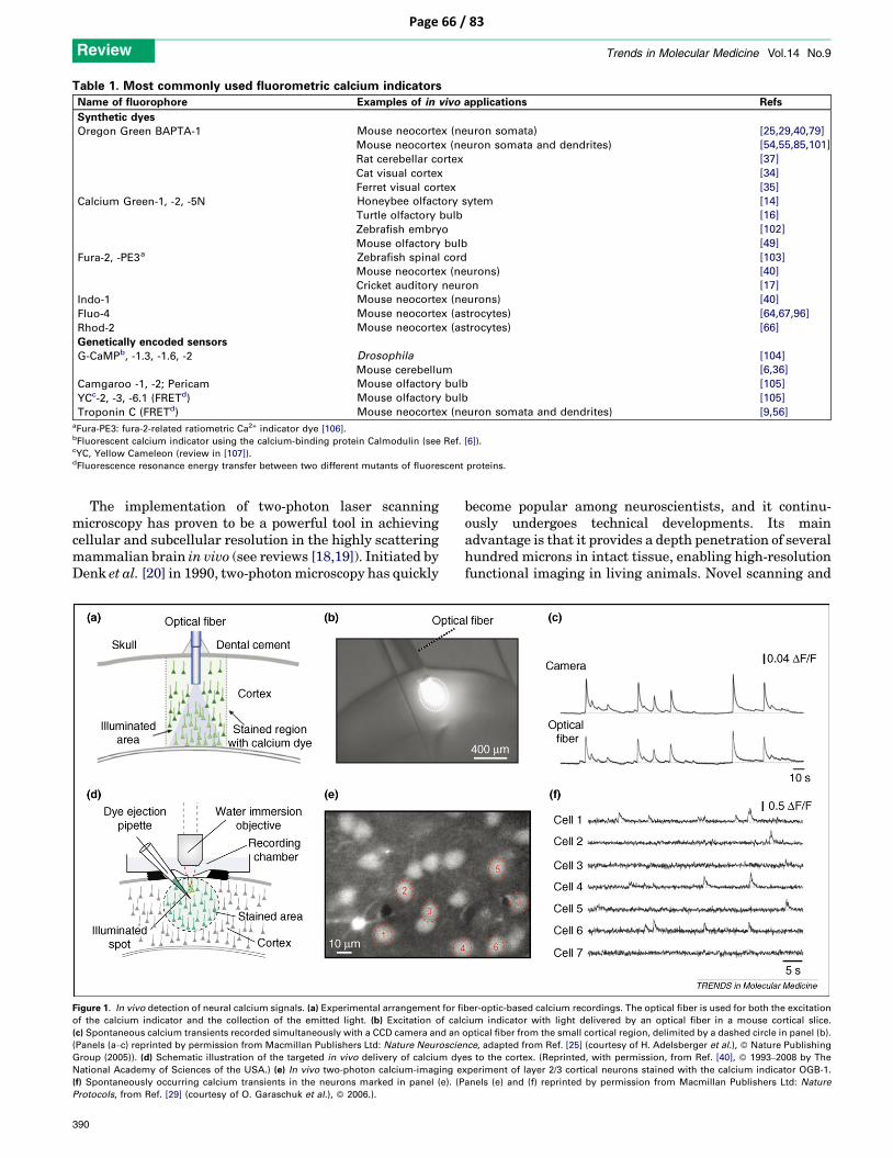
Table 1. Most commonly used fluorometric calcium indicators

Name of fluorophore Examples of in vivo applications Refs

Synthetic dyes

Oregon Green BAPTA-1 Mouse neocortex (neuron somata) [25,29,40,79]

Mouse neocortex (neuron somata and dendrites) [54,55,85,101]

Rat cerebellar cortex [37]

Cat visual cortex [34]

Ferret visual cortex [35]

Calcium Green-1, -2, -5N Honeybee olfactory sytem [14]

Turtle olfactory bulb [16]

Zebrafish embryo [102]

Mouse olfactory bulb [49]

Fura-2, -PE3a Zebrafish spinal cord [103]

Mouse neocortex (neurons) [40]

Cricket auditory neuron [17]

Indo-1 Mouse neocortex (neurons) [40]

Fluo-4 Mouse neocortex (astrocytes) [64,67,96]

Rhod-2 Mouse neocortex (astrocytes) [66]

Genetically encoded sensors

G-CaMPb, -1.3, -1.6, -2 Drosophila [104]

Mouse cerebellum [6,36]

Camgaroo -1, -2; Pericam Mouse olfactory bulb [105]

YCc-2, -3, -6.1 (FRETd) Mouse olfactory bulb [105]

Troponin C (FRETd) Mouse neocortex (neuron somata and dendrites) [9,56]aFura-PE3: fura-2-related ratiometric Ca2+ indicator dye [106].bFluorescent calcium indicator using the calcium-binding protein Calmodulin (see Ref. [6]).cYC, Yellow Cameleon (review in [107]).dFluorescence resonance energy transfer between two different mutants of fluorescent proteins.

Review Trends in Molecular Medicine Vol.14 No.9

Page 66 / 83

The implementation of two-photon laser scanningmicroscopy has proven to be a powerful tool in achievingcellular and subcellular resolution in the highly scatteringmammalian brain in vivo (see reviews [18,19]). Initiated byDenk et al. [20] in 1990, two-photonmicroscopy has quickly

Figure 1. In vivo detection of neural calcium signals. (a) Experimental arrangement for fi

of the calcium indicator and the collection of the emitted light. (b) Excitation of cal

(c) Spontaneous calcium transients recorded simultaneously with a CCD camera and an

(Panels (a–c) reprinted by permission from Macmillan Publishers Ltd: Nature Neuroscie

Group (2005)). (d) Schematic illustration of the targeted in vivo delivery of calcium dy

National Academy of Sciences of the USA.) (e) In vivo two-photon calcium-imaging e

(f) Spontaneously occurring calcium transients in the neurons marked in panel (e). (P

Protocols, from Ref. [29] (courtesy of O. Garaschuk et al.), 2006.).

390

become popular among neuroscientists, and it continu-ously undergoes technical developments. Its mainadvantage is that it provides a depth penetration of severalhundred microns in intact tissue, enabling high-resolutionfunctional imaging in living animals. Novel scanning and

ber-optic-based calcium recordings. The optical fiber is used for both the excitation

cium indicator with light delivered by an optical fiber in a mouse cortical slice.

optical fiber from the small cortical region, delimited by a dashed circle in panel (b).

nce, adapted from Ref. [25] (courtesy of H. Adelsberger et al.), Nature Publishing

es to the cortex. (Reprinted, with permission, from Ref. [40], 1993–2008 by The

xperiment of layer 2/3 cortical neurons stained with the calcium indicator OGB-1.

anels (e) and (f) reprinted by permission from Macmillan Publishers Ltd: Nature

Review Trends in Molecular Medicine Vol.14 No.9

Page 67 / 83

acquisition techniques are being developed for fast time-resolved imaging covering large fields of view and in the 3Dspace [21–23]. The most commonly used stage-mountedmicroscopes for in vivo studies require the head of theanimal to be fixed to minimize motion artifacts. Untilrecently, all imaging studies were performed in head-fixedand anesthetized animals. But a new technique has beenreported for two-photon fluorescence imaging with cellularresolution in awake, behaving head-fixed mice [24], allow-ing the study of brain functions in non-anesthetizedanimals. Another approach for monitoring brain functionsin awake animals involves the use of fiber-optic-basedmicro-endoscopes (Figure 1a–c). Contrary to head-fixedset-ups, this latter approach permits imaging in freelymoving animals. Such endoscopes can be used for signaldetection in deep brain structures, but they have arestricted field of view and low spatial resolution [25].However, this form of imaging has a high temporal resol-ution and reports a compound calcium signal resultingfrom the synchronous activity of small neuronal circuits.Such recordings can be performed in any brain region ofanesthetized and non-anesthetized animals [25]. Animportant goal is the achievement of imaging with cellularresolution through such a microendoscope. One approachis based on the use of micro-electro-mechanical scanners(MEMS) coupled with gradient-index (GRIN) lenses on theoptical fibers [26,27]. Another approach involves the use ofa fiber bundle combined with conventional scanningdevices [28]. To date, however, none of these fiber-optic-based microendoscopy systems have been able to achievean optical image quality that is comparable to that of stage-mounted microscopes and conventional lenses. An im-provement in fiber-optic-based imaging is strongly needed,given that imaging in freely moving animals is ultimatelyrequired in order to address many physiological questionsin in vivo studies.

Imaging neuronal populations activity with cellularresolutionImaging a neuronal population allows the simultaneousmapping of spontaneous and evoked responses of numer-ous cells, from which the function of neuronal circuits canbe inferred. A simple and effective method called multi-cellbolus loading (MCBL) has been developed to deliver acalcium indicator to a large population of intact corticalneurons [18,29]. A concentrated solution of a membrane-permeable acetoxymethyl ester (AM)-form calcium dye, forexample Oregon-Green 488 BAPTA-1 (OGB-1), is injectedby a micropipette into the desired imaging area through asmall skull opening (Figure 1d). After diffusing into thecells, the dye is hydrolyzed by intracellular esterases,making it membrane-impermeable and causing it toremain in the cell while the extracellular dye is washedout (Figure 1e). Calcium signals from multiple cells canthen be imaged with two-photon microscopy (Figure 1f).This method allows the simultaneous recording of largeclusters of neurons and has been successfully applied to theimaging of calcium signals during spontaneous [25] orevoked activity in various brain areas, including the olfac-tory bulb [30–32] (Figure 2a), the visual cortex [33–35](Figure 2b), the cerebellum [36,37] (Figure 2c) and the

somatosensory cortex [38–40] (Figure 2d,e). In the visualcortex of higher mammals, conventional in vivo opticalimaging (optical imaging of intrinsic signals or with vol-tage-sensitive dyes) first demonstrated the existence of anorderly map of preferred stimulus orientations and thearrangement of orientation domains around ‘orientationpinwheels’ [41]. However, the technique lacked the spatialresolution to determine the response properties andarrangement of cells near pinwheel centers. Two-photoncalcium imaging revealed with single-cell resolution thehighly ordered microstructure of pinwheel centers in catvisual cortex [34] (Figure 2b).

The zebrafish is a particularly suitable model for thestudy of the development of sensory systems with in vivocalcium imaging because the larvae are transparent anddevelop rapidly. Two-photon imaging revealed that thedevelopment of retinal ganglion cell axon arbors in theoptic tectum of zebrafish depends on an activity-basedcompetition between neighboring axons [42]. In anotherstudy, two-photon imaging of tectal neurons loaded with afluorescent calcium indicator indicated that soon after thedendritic outgrowth and synaptogenesis, most visual prop-erties in the tectum were already established. The devel-opment of these properties did not require patterned visualexperience [43]. Two-photon calcium imaging in the visualcortex, as well as in the olfactory bulb [31,44,45], of thezebrafish is thus a useful approach for the establishment ofthe functional topology of neuronal activity patterns andthe analysis of the role of activity in circuit developmentand function.

One limitation of the multi-cell bolus loading method isthat it results in a non-specific labeling of all cells, in-cluding all neuronal and glial cells in the stained region.This limitation can be partially overcome by usingadditional specific indicators in parallel. For example,calcium signaling has been studied in cortical astrocyteslabeled with the fluorescent dye sulforhodamine 101 [46]and in GABAergic interneurons expressing enhanced GFP(EGFP) [47]. Another method of labeling a specificneuronal population is to inject into axon bundles a dex-tran-conjugated form of dye, which will then be anterogra-dely and retrogradely transported over hours or days [48].This method has been fruitfully used in the olfactory bulb[49] and in the olivary-cerebellar system [50]. In a studycombining in vivo calcium imaging and retrograde dyelabeling [51], a high variability was revealed in odorant-receptor maps in the olfactory bulb of individual mice (anexample of an odorant-receptormap is shown in Figure 2a).Interestingly, odorant-receptor-defined glomeruli exhib-ited different ligand spectra and far higher sensitivity invivo than in the corresponding in vitro studies [49]. Finally,the problem of imaging specific cell types can be solved byusing genetic targeting of fluorescent protein calcium sen-sors, because the source of the optical signal is specified bythe targeting [6]. For example, transgenic mice expressingthe fluorescent protein calcium indicator GCaMP2 wereused to investigate presynaptic calcium signaling atcerebellar parallel fiber–Purkinje cell synapses in vivo[36]. An example of two-photon fluorescence imaging ofparallel fiber calcium transients is shown in Figure 2c.Despite this progress in the use of genetically encoded

391

Figure 2. Examples of in vivo calcium imaging in different brain areas. (a) Calcium imaging of odorant-evoked responses in odorant-receptor-defined glomeruli (Ea, Eb, Ec

and Ma) in the mouse olfactory bulb. ‘F image’ is the reference image of the brain’s surface. The other images are pseudo-colored representations in which red corresponds

to the largest odor-evoked response. The odorants used are indicated at the top of the images: eugenol (EG), methyl EG (MEG), isoeugenol (IEG), methyl IEG (MIEG),

vanillin (V), acetyl EG (AEG), acetyl IEG (AIEG), benzyl IEG (BIEG), guaiacol (G), 4-hydroxy 3-methyl benzaldehyde (4H3MBA). (Reprinted from Ref. [49] (courtesy of K.

Touhara), 2006 Elsevier Inc., with permission of Elsevier.) (b) (i): Cell-based orientation map in the cat visual cortex obtained with two-photon calcium imaging. Scale bar

represents 100 mm. (ii): Time course of the calcium signals evoked by visual stimulation in three selective cells (1–3) in the pinwheel centre and three selective cells (4–6) in

the iso-orientation domain. Grey bars indicate periods of visual stimulation. (Reprinted by permission from Macmillan Publishers Ltd: Nature, adapted from Ref. [34],

2006 Nature Publishing Group.) (c) Two-photon imaging of parallel fiber calcium transients in the cerebellum of a living GCaMP2 mouse. (i): Image of basal fluorescence,

scale bar represents 50 mm. (ii): Fluorescence signal in response to electrical stimulation via the electrode (indicated as dashed line shape). Green color corresponds to the

largest response (DF/F = 30%). (iii): Composite image of panels (i) and (ii) showing DF/F values. (iv): Time course of the fluorescence response (DF/F). (Reprinted from Ref.

[36] (courtesy of T. Knopfel), 2007 Elsevier Inc., with permission of Elsevier.) (d) Astrocyte-mediated control of cerebral blood flow in the somatosensory cortex. (i): Two-

photon images of a vascular astrocyte (labeled with calcium indicator rhod-2, red) showing calcium increases (yellow) restricted to the endfeet after photolysis of caged

Review Trends in Molecular Medicine Vol.14 No.9

392

Page 68 / 83

Figure 3. Calcium imaging of neuronal dendrites. (a) Schematic representation of the Troponin-C (TnC)-based fluorescence resonance energy transfer (FRET) calcium

indicator CerTN-L15. This genetically encoded calcium indicator is based on changes in FRET efficiency between two different mutants of GFP [8,9]. Abbreviations: CFP,

cyan fluorescent protein; Citrine, citrine-yellow fluorescent protein. (b) In vivo two-photon imaging of neuronal dendrites expressing the genetically encoded calcium

indicator CerTN-L15 (green). Astrocytes were stained with the selective marker sulforhodamine 101 (red). (c) Imaging of a spiny dendrite (i) and FRET calcium signals

evoked by local glutamate application (ii). (Panels (a) and (b) reprinted by permission from Macmillan Publishers Ltd: Cell Calcium, from Ref. [9], Nature Publishing Group

(2007). Panel (c) reprinted from Ref. [56], Elsevier Ltd (2007), with permission of Elsevier.) (d) (i) Reconstruction of a cortical neuron labeled by in vivo electroporation with

the calcium dye OGB1-hexapotassium salt. (ii) Imaging of a portion of dendrite indicated by the red square in (i). (e) In vivo two-photon imaging of spontaneous calcium

signals in the dendritic segments indicated in panel (d).

Review Trends in Molecular Medicine Vol.14 No.9

Page 69 / 83

calcium indicators, the results obtained in vivo in micewere much less impressive than those obtained in fly andfish (e.g. see Ref. [9]). New sensors [52] and, perhaps, otherdelivery methods, for example viral transfection, couldsoon lead to improved in vivo brain calcium imaging inmammals.

Calcium signaling in dendritic compartmentsThe bulk loading approach of calcium indicators (MCBLmethod) is well suited for the analysis of somatic activity inneural circuits. It has limitations when it comes to theimaging of subcellular compartments, such as dendrites,because the image contrast is reduced due to the staining ofmany fine processes in the surrounding neuropil. Further-more, the dye concentration in MCBL-loaded cells is lowerthan in cells stained using a microelectrode [40,53]. These

(Figure 2 continued) calcium, at the position indicated by the arrow. The vasculature wa

endfoot and somatic calcium signals. Scale bar represents 10 mm. (Reprinted by permis

(courtesy of T. Takano), 2006 Nature Publishing Group.) (e) In vivo cortical recordings o

the mouse barrel cortex. (ii): Two-photon line-scan recordings of calcium transients ev

[40], 1993–2008 by The National Academy of Sciences of the USA.).

limitations also reduce the depth resolution of the record-ings to 200–300 mmunder the cortical surface as comparedwith a depth of more than 500 mm when imaging celldendrites of microelectrode-loaded cells [53].

For the detection of calcium signals from dendrites andspines, alternative labeling methods have been used, suchas dye delivery through patch-clamp pipettes [54,55],genetically encoded calcium indicators [56] (Figure 3a–c)and electroporation [57] (Figure 3d,e). These methods,combined with two-photon microscopy, provided the firstimages of dendritic signals in vivo. One application of thisis, for example, the imaging of the propagation of somaticaction potentials back into the dendritic tree in the livingbrain [54,55,58], a process that has previously been exten-sively studied in brain slices [59]. By using both calciumimaging and electrophysiological recordings, the relation-

s stained with FITC-dextran (green). (ii): An astrocyte showing an increase in both

sion from Macmillan Publishers Ltd: Nature Neuroscience, adapted from Ref. [66]

f calcium transients evoked by whisker deflection. (i): Image of layer 2/3 neurons in

oked in two neurons by whisker deflection. (Reprinted, with permission, from Ref.

393

Review Trends in Molecular Medicine Vol.14 No.9

Page 70 / 83

ship between dendritic calcium dynamics and electricalactivities was characterized in themouse brain in vivo [55].However, until recently, single-action potential detectionwas unreliable with imaging approaches, although theestimation of action potential activity from calcium signalsremains a key issue in the study of neuronal networks withcalcium imaging [60,61]. It has recently been shown that itis possible to infer electrical activity with single-cell andsingle-action potential resolution from calcium transientsmeasured in bulk-loaded neuronal populations [38,39,44](see also Box 1 in [61]). Under favorable conditions, spikerates can be estimated from the fluorescence signal by adeconvolution-based method (e.g. see Ref. [44]).

Dendritic compartments represent key elements forsynaptic signal integration [62], but their analysis posesmajor challenges. One difficulty is related to the fact thatthe orientation of the dendrites is mostly not within theusual horizontal XY imaging plane. This problem hasrecently been solved by the implementation of a novelapproach that allows scanning in user-defined imagingplanes [63]. Further improvements are needed to studythe dendritic integration of sensory-evoked signals with ahigher efficiency. For example, an important next stepmight be an approach that facilitates the identificationof dendritic spines that are activated by sensory stimu-lation.

In vivo calcium imaging in disease modelsFor a long time, calcium imaging has been widely appliedfor the study of various neuronal diseases in animalmodelsin vitro, mostly in cell cultures and in brain slices. In recentyears, novel imaging techniques with cellular resolutionhave been increasingly used for the investigation of diseasemodels in vivo with the goal of a detailed characterizationof patho-physiological mechanisms. Because of depth-penetration limitations, optical imaging techniques aremore suitable for studying pathological modifications inneuronal layers near the cortical surface (e.g. in the case ofAlzheimer’s disease) than in deeper brain regions (e.g. inthe case of Parkinson’s disease) and in the grey matterrather than in the white matter. Studies of impaired brainfunctions also greatly benefit from the development of alarge array of genetic tools. Awide range of transgenicmiceis now available, including models of neurological diseasesand/or mice with specific cell types or cellular compart-ments labeled.

Two-photon calcium imaging is a powerful techniquenot only for studying neuronal activity but also for studyingelectrically non-excitable glial cells, for example astro-cytes, in vivo [64]. Astrocytes are involved in many normaland pathological brain functions and represent a promis-ing target for therapeutic treatments. Recent in vivo stu-dies indicated that astrocytes show rapid increase incalcium upon sensory stimulation [35,65], have a role inregulating arterial blood flow [66] and are implicated inepilepsy [67,68], stroke and Alzheimer’s disease [69].Astrocytes can be readily labeled in vivo by the red fluor-escent indicator sulforhodamine 101 [70], as well as byvarious transgenic labels [71]. In addition to the imaging ofneuronal and glial activity, two-photon microscopy alsooffers the possibility to image the development of patho-

394

logical protein aggregates, such as tangles and senileplaques in Alzheimer’s disease, and to follow how theyreact to therapeutic treatments.

Alzheimer’s disease, aging and degeneration

Alzheimer’s disease is a degenerative and terminal dis-ease for which there is currently no known cure. It isconsidered to be the most common cause of adult demen-tia. The cause and progression of Alzheimer’s disease isnot well understood but is associated with senile plaques[extracellular deposits of amyloid b (Ab) peptide] andneurofibrillary tangles (intracellular accumulations of ahyperphosphorylated form of microtubule-associated tauprotein) in the brain [72]. Several mouse models ofAlzheimer’s disease exist [73,74] in which Ab plaquescan be labeled in vivo via: (i) fluorescent dyes, such asthioflavin-S; (ii) fluorescently labeled antibodies againstAb [75]; or (iii) intravenous (or even intraperitoneal)injection of a lipophilic Congo red derivative (Methoxy-X04) that can cross the blood–brain barrier and staincerebrovascular as well as plaque-bound Ab [76,77]. Byimaging both plaques and neurons in vivo with two-photon microscopy, it is then possible to explore howAb plaques contribute to neuronal damage. One way is toperform morphological studies using transgenic micewith cells that are stained with fluorescent proteins. Arecent longitudinal in vivo two-photon microscopy studyshowed the rapid appearance and local toxicity of Ab

plaques within only a few days, leading to increasinglydysmorphic neurites [77]. This fast timing was notexpected because predictions were based on in vitrostudies in which the appearance of Ab aggregationswas more protracted and followed a relatively slownucleation-dependent polymerization process.

Glial cells are also believed to be strongly involved in thedevelopment of Alzheimer’s disease pathology and can alsobe studied in vivo. For example, it was shown that one ortwo days after a new plaque’s appearance, microglia areactivated and recruited to the site [77]. Two-photon in vivoimaging of astrocytic calcium signaling in experimentalmouse models of Alzheimer’s disease revealed that abnor-mal astrocytic activity and instability in the microcircula-tion occurs in early stages of the disease preceding Ab

deposition and neuronal loss [69].In such disease models, to study the impairment of local

neuronal functions and their potential recovery aftertherapeutic treatments, functional recordings arerequired, either by electrophysiology [78] or by calciumimaging. Recently, it has been shown that calcium signalscan be recorded fromneurons around plaques in transgenicAlzheimer’s disease mice [79]. The combination of themulti-cell bolus loading method and multicolor in vivotwo-photon imaging allows the simultaneous studying ofneurons, glial cells and senile plaques in the cortex of aged(up to two years old)mice [79] (see Figure 4a). The presenceof lipofuscin and a lower imaging contrast make quanti-tative calcium measurements in aged tissue more difficultthan in young mice, but recordings are still possible. Infact, in vivo calcium imaging in aged tissue is by farsuperior to any other type of registration because of therapid degradation of this tissue under in vitro conditions.

Figure 4. Examples of in vivo calcium imaging in brain disease models. (a) (i): In vivo two-photon imaging of neurons stained with OGB-1 (green) in the cortical layer 2/3 of

a 15-month-old transgenic mouse expressing EGFP in microglial cells (red). (ii): Triple staining of cortical layer 2/3 cells with OGB-1 (green), thioflavine-S (Ab plaques, cyan)

and sulforhodamine 101 (astrocytes, red). (iii): Imaging of lipofuscin autofluorescence (red) in a transgenic mouse expressing EGFP in microglial cells (green). Note large

lipofuscin deposits within the microglia cell body (arrowheads). Scale bars represent 10 mm. (Adapted from Ref. [79] (courtesy of O. Garaschuk et al.) with kind permission

from Springer Science+Business Media, Springer-Verlag 2007.) (b) Changes in intracellular calcium levels in vivo during transient ischemia coincide with slow

electroencephalogram (DC EEG) activity and dendritic beading. (i): Change in normalized OGB-1 fluorescence taken from the neuropil in cortical layer I and cortical DC EEG

recording of an animal subjected to bilateral common carotid artery ligation and reperfusion (Reper). (ii): GFP-labeled dendrites surrounded by diffuse OGB-1-labeled layer I

neuropil from the same animal. At 206 s after ischemic onset, the layer I neuropil shows a large increase in OGB-1 fluorescence, indicating a sudden rise in intracellular

calcium. The dendrites have become severely blebbed. At 2 min after reperfusion (514 s after ischemic onset), neuropil OGB-1 fluorescence levels are already beginning to

decline, and 13 min (738 s) after ischemia the dendritic structure is nearly fully restored. (Adapted from Ref. [85] (courtesy of T.H. Murphy) with permission of 2008

Society for Neuroscience.) (c) Experimental epileptic seizures in adult mice. (i): The primary somatosensory cortex was loaded with the astrocyte-specific dye

sulforhodamine 101 (SR101) and the calcium indicator fluo-4 AM. Note that fluo-4 AM was preferentially taken up by astrocytes. Scale bar represents 25 mm. (ii): In vivo two-

photon imaging showed abnormal calcium signaling (increase in fluo-4 emission in second image from left) preceding epileptiform discharges induced by the delivery of 4-

aminopyridine (4-AP). The field potential recording showed an epileptiform event induced by 4-AP. Lower traces correspond to expanded recordings during the periods

indicated by dotted lines. (Reprinted by permission from Macmillan Publishers Ltd: Nature Medicine, adapted from Ref. [67] (courtesy of G.F. Tian), 2005 Nature

Publishing Group.).

Review Trends in Molecular Medicine Vol.14 No.9

Page 71 / 83

Amyotrophic lateral sclerosis (ALS) is another progress-ive neurodegenerative disease that could be studied bycalcium imaging in a mouse model. The disease is charac-terized by a substantial loss of motor neurons in the spinalcord, brain stem and motor cortex. In vivo microscopyrevealed early pathological changes of synaptic trans-mission in an ALS mouse model with transgenic yellowfluorescent protein expressed in all or subsets of motorneurons [80]. In vitro calcium imaging was performed incultured spinal cordmotor neurons of an ALSmousemodel[81]. The implementation of two-photon calcium imagingin vivo is feasible and should decisively advance the inves-tigation of the pathophysiological mechanisms underlyingthis disease.

Stroke, ischemia and hypoxia

Stroke is the rapid loss of brain functions in response to acerebrovascular dysfunction. This dysfunction can be

caused by either hemorrhage or ischemia (lack of bloodsupply) due to thrombosis or embolism. By using in vivotwo-photon imaging, blood vessels can be visualized byintravenous injection of fluorescent dextran conjugates(Figure 2d) and blood flow can be measured by imagingthe negative contrast of erythrocytes that exclude thedextran. Visualization of stimulus-induced changes incapillary flow was one of the first applications of two-photon microscopy in vivo [82]. Because ischemia can beeasily induced in animals, this approach has subsequentlybeen used to study animal models of ischemic stroke. Byusing GFP-expressing transgenic mice, it was observedthat severe ischemia leads to rapid dendritic spine lossand alterations that could be substantially recovered ifreperfusion occurred within 20–60 min [83]. The extent ofthe functional recovery after restoration of normal bloodflow was studied with the same approach combined withoptical imaging of intrinsic signals [84]. The mouse model

395

Review Trends in Molecular Medicine Vol.14 No.9

Page 72 / 83

of ischemia has been further improved to alternate rapidlybetween the initiation of ischemia and reperfusion. Two-photon calcium imaging and optical imaging of intrinsicsignals were used in this improved model to study func-tionally the initial reversible events associated with ische-mia [85]. The new approach revealed that the apicaldendritic structure of layer V neurons in the mouse soma-tosensory cortex was dramatically degraded by globalischemia. A key factor of this impairment was a propagat-ing, spreading-depression-like ischemic depolarizationthat enveloped the cortex 2–3 min after ischemic onsetand that occurred independently of ionotropic glutamatereceptors [85]. Increases in intracellular calcium levelsoccurred during the wave of ischemic depolarization andwere coincident with the loss of dendritic structure (seeFigure 4b). After reperfusion, the dendritic structure, theintracellular calcium levels and the somatosensory func-tions largely recovered to the same status as before thesebrief periods of ischemia (6–8 min).

Spreading depression is a neural dysfunction that isoften associated with migraine and with progressiveneuronal injury after stroke and head trauma [86,87].Two-photon calcium imaging showed that spreadingdepression was correlated with neuronal and astrocyticcalcium waves and with the constriction of intracorticalarterioles that could arrest capillary perfusion [86]. In vivotwo-photon microscopy was used in a similar model ofspreading depression to perform quantitative metabolicimaging. This was achieved by imaging, instead of calcium,the reduced form of nicotinamide adenine dinucleotide(NADH), a coenzyme found in all living cells. IntrinsicNADH tissue fluorescence served as a sensitive indicatorof the cellular redox state in vivo. This study showed thatspreading depression is associated with severe hypoxiaand neuronal swelling [87].

The control of cerebral blood flow was also investigatedin non-pathological conditions. The mechanism by whichlocal electrical activity is translated into increases in bloodflow remains poorly understood, although many in vivofunctional imaging methods, such as functional magneticresonance imaging (fMRI), are based on this coupling. Therole of astrocytes in vasoregulation was studied in vitro,but conflicting results were obtained in different studies[88,89]. An in vivo approach was clearly needed to studyregulation of cerebral blood flow because there is no bloodcirculation in brain slices. Two-photon in vivo calciumimaging in combination with local uncaging of cagedcalcium revealed a critical role of astrocytes in the controlof local microcirculation (see Figure 2d) [66]. In addition,the relationship between neuronal activity and localcerebral blood flow was recently investigated in the rodentolfactory bulb [90].

Epilepsy

Epilepsy is a common neurological disorder that is charac-terized by recurrent seizures caused by bursts of synchro-nous, rhythmic neuronal hyperactivity. The problems ofthe initiation and propagation of the seizures as well as theinjuries caused by these seizures on neuronal functions arestill not entirely understood. The standard methods formonitoring epileptic activity – surface electrophysiological

396

recordings or functional imaging techniques, such as fMRIand positron-emission tomography – generally lack eitherthe spatial or temporal resolution to study seizure activityand neuronal impairments at the cellular level. The first invivo studies used imaging of intrinsic optical signals tomonitor neuronal activity during and after epileptic events[91]. After establishing the technique in an animal model(ferret), this approach was used to generate maps of epi-leptiform or physiological activity in the human cortex [92].However, imaging of intrinsic optical signals does not allowanalysis at the cellular level. Thus, two-photon imagingwas used in models of epileptic seizures, first in vitro, inbrain slices [93], and then in vivo in combination with theuse of GFP-expressing transgenic mice [94]. With thisapproach, acute dendritic injury caused by kainate sei-zures could be studied in vivo [95].

Calcium imaging in vivo was used for the investigationof astrocytic activity during epileptic events. In vivo two-photon imaging showed that astrocytic calcium eventswere strongly correlated with the epileptogenic neuronalbursting activity induced by the administration of 4-aminopyridine (a potassium channel blocker that inducesseizure activity in experimental models) [67,96] (seeFigure 4c). Furthermore, anti-epileptic drugs, such asvalproate, gabapentin and phenytoin, reduced both theamplitude of neuronal discharges and astrocytic calciumsignaling induced by 4-aminopyridine [67]. These resultssuggest that epileptic discharges are secondary to the glialpathology and that astrocytes might represent a promisingnew target for treatments of epilepsy. In vivo two-photoncalcium imaging can thus be an effective tool for theidentification of unknown cellular elements involved inbrain pathologies and can help reveal new therapeutictargets. A recent study introduced an in vivo model ofdevelopmental seizures within the intact unanesthetizedbrain of the transparent albinoXenopus laevis tadpole [97].Pentylenetetrazol-induced seizures were characterizedusing in vivo two-photon calcium imaging of neuronaldynamics in this simple animal model preparation [97].

ConclusionsCalcium imaging in the living brain, especially two-photonimaging in the mouse brain, is increasingly being used forthe analysis of various animal disease models. In particu-lar, neurodegenerative-disease research benefits from invivo investigations because many previous in vitro studieswith nervous tissue from old animals did not providesatisfactory results. It is important to remember that evenin healthy animals, good quality in vitro brain slices aremostly obtained at relatively early developmental stages.By contrast, in vivo two-photon calcium imaging exper-iments are feasible and produce good results in both youngand aged mice (e.g. Ref [79]).

Although two-photon microscopy provides a betterdepth penetration than wide-field and confocal microscopy[19], in vivo two-photon imaging experiments are stillmostly restricted to the exploration of superficial brainlayers in the neocortex [18,39], cerebellum [36,37] andolfactory bulb [30–32] (Box 1). Recordings in deeper brainstructures will require different technologies. New andpromising approaches for microendoscopical recordings

Box 1. Outstanding questions that can be addressed with

in vivo calcium imaging

In the brain of Alzheimer’s disease animal models, what are the

functional changes of neuron activity in plaque-rich regions?

How do neurons function in the aged brain? How do the functions

of neural circuits change with age?

How does neuronal plasticity underlying learning and memory

change during the development of the brain?

What is the function of genetically defined classes of neurons (e.g.

parvalbumin-containing inhibitory neurons) in the normal and

diseased (epileptic) brain?

How do antiepileptic drugs affect the function of specific types of

neurons (excitatory vs inhibitory) of the same cortical micro-

circuit?

How does the cell-specific genetic modification of neurons (e.g.

that of Purkinje neurons in the cerebellum) affect the function of

the neural circuit and cause disease (e.g. ataxia)?

Review Trends in Molecular Medicine Vol.14 No.9

Page 73 / 83

are under way. These include single fiber volumetricrecordings [25], fiber-bundle-based confocal imaging [98]and two-photon imaging using the GRIN lens technology[99,100]. With these new methods, the exploration of dis-eases, such as Parkinson’s disease and Huntington’s dis-ease, that are caused by impairments in deeper brain areaswill soon be possible in in vivo animal models.

AcknowledgementsSupported by the Deutsche Forschungsgemeinschaft (IRTG 1373) and theSchiedel Foundation. A.K. is a Carl-von-Linde Senior Fellow of theInstitute for Advanced Study of the TUM.

References1 Ramon y Cajal, S. (1909, 1911) Histologie du Systeme Nerveux de

l’Homme et des Vertebres (French edition reviewed and updated by theauthor, translated from Spanish by L. Azoulay), Maloine, Paris[published in English in 1995 as Histology of the Nervous System ofMan and Vertebrates (translated by N. Swanson and L.W. Swanson),Oxford University Press]

2 Tsien, R.Y. (1989) Fluorescent probes of cell signaling. Annu. Rev.Neurosci. 12, 227–253

3 Tsien, R.Y. (1998) The green fluorescent protein. Annu. Rev. Biochem.67, 509–544

4 Miyawaki, A. (2005) Innovations in the imaging of brain functionsusing fluorescent proteins. Neuron 48, 189–199

5 Mao, T. et al. (2008) Characterization and subcellular targeting ofGCaMP-type genetically-encoded calcium indicators. PLoS ONE 3,e1796

6 Knopfel, T. et al. (2006) Optical probing of neuronal circuit dynamics:genetically encoded versus classical fluorescent sensors. TrendsNeurosci. 29, 160–166

7 Kotlikoff, M.I. (2007) Genetically encoded Ca2+ indicators: usinggenetics and molecular design to understand complex physiology.J. Physiol. 578, 55–67

8 Shimozono, S. and Miyawaki, A. (2008) Engineering FRET constructsusing CFP and YFP. Methods Cell Biol. 85, 381–393

9 Garaschuk, O. et al. (2007) Troponin C-based biosensors: a new familyof genetically encoded indicators for in vivo calcium imaging in thenervous system. Cell Calcium 42, 351–361

10 Connor, J.A. (1986) Digital imaging of free calcium changes and ofspatial gradients in growing processes in single, mammaliancentral nervous system cells. Proc. Natl. Acad. Sci. U. S. A. 83,6179–6183

11 Tank, D.W. et al. (1988) Spatially resolved calcium dynamicsof mammalian Purkinje cells in cerebellar slice. Science 242, 773–

77712 Egelhaaf, M. et al. (2002) Neural encoding of behaviourally relevant

visual-motion information in the fly. Trends Neurosci. 25, 96–10213 Helmchen, F. and Waters, J. (2002) Ca2+ imaging in the mammalian

brain in vivo. Eur. J. Pharmacol. 447, 119–129

14 Galizia, C.G. et al. (1999) The glomerular code for odor representationis species specific in the honeybee Apis mellifera. Nat. Neurosci. 2,473–478

15 Wang, Y. et al. (2001) Genetic manipulation of the odor-evokeddistributed neural activity in the Drosophila mushroom body.Neuron 29, 267–276

16 Wachowiak, M. et al. (2002) Distributed and concentration-invariantspatial representations of odorants by receptor neuron input to theturtle olfactory bulb. J. Neurophysiol. 87, 1035–1045

17 Sobel, E.C. and Tank, D.W. (1994) In vivo Ca2+ dynamics in a cricketauditory neuron: an example of chemical computation. Science 263,823–826

18 Garaschuk, O. et al. (2006) Optical monitoring of brain function invivo: from neurons to networks. Pflugers Arch. 453, 385–396

19 Helmchen, F. and Denk, W. (2005) Deep tissue two-photonmicroscopy. Nat. Methods 2, 932–940

20 Denk, W. et al. (1990) Two-photon laser scanning fluorescencemicroscopy. Science 248, 73–76

21 Duemani Reddy, G. et al. (2008) Three-dimensional random accessmultiphoton microscopy for functional imaging of neuronal activity.Nat. Neurosci. 11, 713–720

22 Gobel, W. et al. (2007) Imaging cellular network dynamics in threedimensions using fast 3D laser scanning. Nat. Methods 4, 73–79

23 Salome, R. et al. (2006) Ultrafast random-access scanning in two-photon microscopy using acousto-optic deflectors. J. Neurosci.Methods 154, 161–174

24 Dombeck, D.A. et al. (2007) Imaging large-scale neural activity withcellular resolution in awake, mobile mice. Neuron 56, 43–57

25 Adelsberger, H. et al. (2005) Cortical calcium waves in restingnewborn mice. Nat. Neurosci. 8, 988–990

26 Flusberg, B.A. et al. (2005) In vivo brain imaging using a portable3.9 gram two-photon fluorescence microendoscope. Opt. Lett. 30,2272–2274

27 Mehta, A.D. et al. (2004) Fiber optic in vivo imaging in themammaliannervous system. Curr. Opin. Neurobiol. 14, 617–628

28 Gobel, W. et al. (2004) Miniaturized two-photonmicroscope based on aflexible coherent fiber bundle and a gradient-index lens objective.Opt.Lett. 29, 2521–2523

29 Garaschuk, O. et al. (2006) Targeted bulk-loading of fluorescentindicators for two-photon brain imaging in vivo. Nat Protoc. 1, 380–

38630 Tabor, R. et al. (2004) Processing of odor mixtures in the zebrafish

olfactory bulb. J. Neurosci. 24, 6611–662031 Wachowiak, M. et al. (2004) Functional organization of sensory input

to the olfactory bulb glomerulus analyzed by two-photon calciumimaging. Proc. Natl. Acad. Sci. U. S. A. 101, 9097–9102

32 Charpak, S. et al. (2001) Odor-evoked calcium signals in dendrites ofrat mitral cells. Proc. Natl. Acad. Sci. U. S. A. 98, 1230–1234

33 Mrsic-Flogel, T.D. et al. (2007) Homeostatic regulation of eye-specificresponses in visual cortex during ocular dominance plasticity.Neuron54, 961–972

34 Ohki, K. et al. (2006) Highly ordered arrangement of single neurons inorientation pinwheels. Nature 442, 925–928

35 Schummers, J. et al. (2008) Tuned responses of astrocytes and theirinfluence on hemodynamic signals in the visual cortex. Science 320,1638–1643

36 Diez-Garcia, J. et al. (2007) In vivo calcium imaging from geneticallyspecified target cells in mouse cerebellum. Neuroimage 34, 859–

86937 Sullivan, M.R. et al. (2005) In vivo calcium imaging of circuit activity

in cerebellar cortex. J. Neurophysiol. 94, 1636–164438 Kerr, J.N. et al. (2007) Spatial organization of neuronal population

responses in layer 2/3 of rat barrel cortex. J. Neurosci. 27, 13316–

1332839 Sato, T.R. et al. (2007) The functional microarchitecture of the mouse

barrel cortex. PLoS Biol. 5, e18940 Stosiek, C. et al. (2003) In vivo two-photon calcium imaging of

neuronal networks. Proc. Natl. Acad. Sci. U. S. A. 100, 7319–732441 Bonhoeffer, T. and Grinvald, A. (1991) Iso-orientation domains in cat

visual cortex are arranged in pinwheel-like patterns. Nature 353,429–431

42 Hua, J.Y. et al. (2005) Regulation of axon growth in vivo by activity-based competition. Nature 434, 1022–1026

397

Review Trends in Molecular Medicine Vol.14 No.9

Page 74 / 83

43 Niell, C.M. and Smith, S.J. (2005) Functional imaging reveals rapiddevelopment of visual response properties in the zebrafish tectum.Neuron 45, 941–951

44 Yaksi, E. and Friedrich, R.W. (2006) Reconstruction of firing ratechanges across neuronal populations by temporally deconvolved Ca2+

imaging. Nat. Methods 3, 377–38345 Yaksi, E. et al. (2007) Topological reorganization of odor

representations in the olfactory bulb. PLoS Biol. 5, e17846 Winship, I.R. et al. (2007) Rapid astrocyte calcium signals correlate

with neuronal activity and onset of the hemodynamic response in vivo.J. Neurosci. 27, 6268–6272

47 Sohya, K. et al. (2007) GABAergic neurons are less selective tostimulus orientation than excitatory neurons in layer II/III ofvisual cortex, as revealed by in vivo functional Ca2+ imaging intransgenic mice. J. Neurosci. 27, 2145–2149

48 Hirase, H. et al. (2004) Two-photon imaging of brain pericytes in vivousing dextran-conjugated dyes. Glia 46, 95–100

49 Oka, Y. et al. (2006) Odorant receptormap in themouse olfactory bulb:in vivo sensitivity and specificity of receptor-defined glomeruli.Neuron 52, 857–869

50 Kreitzer, A.C. et al. (2000) Monitoring presynaptic calcium dynamicsin projection fibers by in vivo loading of a novel calcium indicator.Neuron 27, 25–32

51 Durand, G.M. et al. (2006) Quantitative single-cell RT-PCR and Ca2+

imaging in brain slices. Pflugers Arch. 451, 716–72652 Mank, M. and Griesbeck, O. (2008) Genetically encoded calcium

indicators. Chem. Rev. 108, 1550–156453 Svoboda, K. et al. (1997) In vivo dendritic calcium dynamics in

neocortical pyramidal neurons. Nature 385, 161–16554 Helmchen, F. et al. (1999) In vivo dendritic calcium dynamics in deep-

layer cortical pyramidal neurons. Nat. Neurosci. 2, 989–99655 Svoboda, K. et al. (1999) Spread of dendritic excitation in layer

2/3 pyramidal neurons in rat barrel cortex in vivo. Nat. Neurosci.2, 65–73

56 Heim, N. et al. (2007) Improved calcium imaging in transgenicmice expressing a troponinC-based biosensor.Nat.Methods 4, 127–129

57 Nagayama, S. et al. (2007) In vivo simultaneous tracing and Ca2+

imaging of local neuronal circuits. Neuron 53, 789–80358 Waters, J. and Helmchen, F. (2004) Boosting of action potential

backpropagation by neocortical network activity in vivo. J. Neurosci.24, 11127–11136

59 Stuart, G. et al. (1997) Action potential initiation andbackpropagation in neurons of the mammalian CNS. TrendsNeurosci. 20, 125–131

60 Gobel, W. and Helmchen, F. (2007) In vivo calcium imaging of neuralnetwork function. Physiology (Bethesda) 22, 358–365

61 Kerr, J.N. and Denk, W. (2008) Imaging in vivo: watching the brain inaction. Nat. Rev. Neurosci. 9, 195–205

62 Eilers, J. and Konnerth, A. (1997) Dendritic signal integration. Curr.Opin. Neurobiol. 7, 385–390

63 Gobel, W. and Helmchen, F. (2007) New angles on neuronal dendritesin vivo. J. Neurophysiol. 98, 3770–3779

64 Hirase, H. et al. (2004) Calcium dynamics of cortical astrocyticnetworks in vivo. PLoS Biol. 2, e96

65 Wang, X. et al. (2006) Astrocytic Ca2+ signaling evoked by sensorystimulation in vivo. Nat. Neurosci. 9, 816–823

66 Takano, T. et al. (2006) Astrocyte-mediated control of cerebral bloodflow. Nat. Neurosci. 9, 260–267

67 Tian, G.F. et al. (2005) An astrocytic basis of epilepsy. Nat. Med. 11,973–981

68 Oberheim, N.A. et al. (2008) Loss of astrocytic domain organization inthe epileptic brain. J. Neurosci. 28, 3264–3276

69 Takano, T. et al. (2007) Two-photon imaging of astrocytic Ca2+signaling and the microvasculature in experimental mice models ofAlzheimer’s disease. Ann. N. Y. Acad. Sci. 1097, 40–50

70 Nimmerjahn, A. et al. (2004) Sulforhodamine 101 as a specificmarker of astroglia in the neocortex in vivo. Nat. Methods 1, 31–37

71 Nolte, C. et al. (2001) GFAP promoter-controlled EGFP-expressingtransgenicmice: a tool to visualize astrocytes and astrogliosis in livingbrain tissue. Glia 33, 72–86

72 Haass, C. and Selkoe, D.J. (2007) Soluble protein oligomers inneurodegeneration: lessons from the Alzheimer’s amyloid b-peptide. Nat. Rev. Mol. Cell Biol. 8, 101–112

398

73 Oddo, S. et al. (2003) Triple-transgenic model of Alzheimer’s diseasewith plaques and tangles: intracellular Ab and synaptic dysfunction.Neuron 39, 409–421

74 Sturchler-Pierrat, C. and Sommer, B. (1999) Transgenic animals inAlzheimer’s disease research. Rev. Neurosci. 10, 15–24

75 Bacskai, B.J. et al. (2001) Imaging of amyloid-b deposits in brains ofliving mice permits direct observation of clearance of plaques withimmunotherapy. Nat. Med. 7, 369–372

76 Klunk,W.E. et al. (2002) Imaging Ab plaques in living transgenicmicewith multiphoton microscopy and methoxy-X04, a systemicallyadministered Congo red derivative. J. Neuropathol. Exp. Neurol.61, 797–805

77 Meyer-Luehmann,M. et al. (2008) Rapid appearance and local toxicityof amyloid-b plaques in a mouse model of Alzheimer’s disease.Nature451, 720–724

78 Stern, E.A. et al. (2004) Cortical synaptic integration in vivo isdisrupted by amyloid-b plaques. J. Neurosci. 24, 4535–4540

79 Eichhoff, G. et al. (2008) In vivo calcium imaging of the aging anddiseased brain. Eur. J. Nucl. Med. Mol. Imaging 35 (Suppl. 1), S99–

S10680 Schaefer, A.M. et al. (2005) A compensatory subpopulation of motor

neurons in a mouse model of amyotrophic lateral sclerosis. J. Comp.Neurol. 490, 209–219

81 Guatteo, E. et al. (2007) Altered calcium homeostasis in motorneurons following AMPA receptor but not voltage-dependentcalcium channels’ activation in a genetic model of amyotrophiclateral sclerosis. Neurobiol. Dis. 28, 90–100

82 Kleinfeld, D. et al. (1998) Fluctuations and stimulus-inducedchanges in blood flow observed in individual capillaries in layers 2through 4 of rat neocortex. Proc. Natl. Acad. Sci. U. S. A. 95, 15741–

1574683 Zhang, S. et al. (2005) Rapid reversible changes in dendritic spine

structure in vivo gated by the degree of ischemia. J. Neurosci. 25,5333–5338

84 Zhang, S. and Murphy, T.H. (2007) Imaging the impact of corticalmicrocirculation on synaptic structure and sensory-evokedhemodynamic responses in vivo. PLoS Biol. 5, e119

85 Murphy, T.H. et al. (2008) Two-photon imaging of stroke onset in vivoreveals that NMDA-receptor independent ischemic depolarization isthe major cause of rapid reversible damage to dendrites and spines.J. Neurosci. 28, 1756–1772

86 Chuquet, J. et al. (2007) High-resolution in vivo imaging of theneurovascular unit during spreading depression. J. Neurosci. 27,4036–4044

87 Takano, T. et al. (2007) Cortical spreading depression causes andcoincides with tissue hypoxia. Nat. Neurosci. 10, 754–762

88 Mulligan, S.J. and MacVicar, B.A. (2004) Calcium transients inastrocyte endfeet cause cerebrovascular constrictions. Nature 431,195–199

89 Zonta, M. et al. (2003) Neuron-to-astrocyte signaling is central tothe dynamic control of brain microcirculation. Nat. Neurosci. 6, 43–

5090 Chaigneau, E. et al. (2007) The relationship between blood flow and

neuronal activity in the rodent olfactory bulb. J. Neurosci. 27, 6452–

646091 Schwartz, T.H. and Bonhoeffer, T. (2001) In vivo optical mapping of

epileptic foci and surround inhibition in ferret cerebral cortex. Nat.Med. 7, 1063–1067

92 Haglund, M.M. and Hochman, D.W. (2004) Optical imaging ofepileptiform activity in human neocortex. Epilepsia 45 (Suppl. 4),43–47

93 Badea, T. et al. (2001) Calcium imaging of epileptiform events withsingle-cell resolution. J. Neurobiol. 48, 215–227

94 Mizrahi, A. et al. (2004) High-resolution in vivo imaging ofhippocampal dendrites and spines. J. Neurosci. 24, 3147–3151

95 Zeng, L.H. et al. (2007) Kainate seizures cause acute dendriticinjury and actin depolymerization in vivo. J. Neurosci. 27, 11604–

1161396 Tian, G.F. et al. (2006) Imaging of cortical astrocytes using 2-photon

laser scanning microscopy in the intact mouse brain. Adv. Drug Deliv.Rev. 58, 773–787

97 Hewapathirane, D.S. et al. (2008) In vivo imaging of seizure activity ina novel developmental seizure model. Exp. Neurol. 211, 480–488

Review Trends in Molecular Medicine Vol.14 No.9

Page 75 / 83

98 Davenne, M. et al. (2005) In vivo imaging of migrating neurons in themammalian forebrain. Chem. Senses 30 (Suppl. 1), i115–i116

99 Murayama, M. et al. (2007) Fiberoptic system for recording dendriticcalcium signals in layer 5 neocortical pyramidal cells in freely movingrats. J. Neurophysiol. 98, 1791–1805

100 Flusberg, B.A. et al. (2005) Fiber-optic fluorescence imaging. Nat.Methods 2, 941–950

101 Nevian, T. and Helmchen, F. (2007) Calcium indicator loadingof neurons using single-cell electroporation. Pflugers Arch. 454,675–688

102 Ashworth, R. et al. (2001) Buffering intracellular calcium disruptsmotoneuron development in intact zebrafish embryos.Brain Res. Dev.Brain Res. 129, 169–179

103 Brustein, E. et al. (2003) In vivo monitoring of neuronal networkactivity in zebrafish by two-photon Ca2+ imaging. Pflugers Arch. 446,766–773

104 Marella, S. et al. (2006) Imaging taste responses in the fly brain revealsa functional map of taste category and behavior. Neuron 49, 285–295

105 Hasan, M.T. et al. (2004) Functional fluorescent Ca2+ indicatorproteins in transgenic mice under TET control. PLoS Biol. 2, e163

106 Vorndran, C. et al. (1995) New fluorescent calcium indicatorsdesigned for cytosolic retention or measuring calcium nearmembranes. Biophys. J. 69, 2112–2124

107 Palmer, A.E. and Tsien, R.Y. (2006) Measuring calcium signalingusing genetically targetable fluorescent indicators. Nat. Protoc. 1,1057–1065

399

6 Other activities: Custom built video‐rate two‐photon microscopy

setup

The studies of sensory evoked dendritic input sites in vivo as shown in previous chapters 2‐4 had

employed the combined method of two‐photon calcium imaging and whole‐cell recording.

While techniques of whole‐cell recording have been since long well established (1), techniques

of two‐photon imaging still have great potentials to be explored. One important issue of two‐

photon microscopy is the laser scanning (2), i.e., the laser beam must be steered such that the

trajectory of focus points covering the desired field within the optical focal plane. The scanning

can involve either galvanic mirror or AOD‐based scanners. In either case the focus point is

driven simultaneously along two orthogonal axes. Typically, the driving along the horizontal axis

is fast, while the driving along the vertical axis is slower and uniformly spreads the horizontal

lines into a square frame.

In order to acquire an image with sufficient digital resolution, a minimum number of

horizontal lines must be scanned; therefore the repetition rate of image is largely dependent on

the repetition rate of horizontal lines. The most commonly used scanner in confocal and multi‐

photon imaging is the linear galvanometric mirror, which can rotate to angles linearly with the

command voltage. The cycling frequency can typically achieve up to 1 kHz, which means 2 kHz

repetition rate of horizontal scan lines, since one cycle consists of forward and backward lines

and both can be used for image formation. This means that when using 400 lines for the

acquisition of an image, the image repetition rate is maximally 5 frames/s. However, for the

detection of biological signals it is often necessary to use higher sampling rates. For example,

even the accurate imaging of the fine structure of dendrites in vivo may require significantly

higher frame rates, because of the noise resulting from the heart beat‐mediated pulsations of

around 8 Hz (for mice). According to the Nyquist‐Shannon sampling theorem (3), in order to be

able to acquire information of this noise and numerically filter it, the imaging speed should be

above two‐fold of it, i.e., 16 frames/s for the case of imaging dendrites located near a pulsating

blood vessel.

Page 76 / 83

One solution for increasing the imaging frame rate is to replace the linear galvanometric

mirror by a resonant mirror for the horizontal axis (4). The cycling frequency of resonant mirror

is typically 8 kHz so the gain of frame rate is about 8‐fold. For example as shown in chapter 2, a

configuration of 400 lines x 30 frames/s were used for recording visually evoked hotspots in

multiple (2‐8) dendritic portions (10‐80 µm length each) of single layer 2 neuron in mouse visual

cortex. Furthermore, I have implemented a 12 kHz resonant scanner (typically configured at 512

lines x 40 frames/s) which was successfully used for imaging dendritic spines in cortical neurons

of the vibrissal cortex in vivo, as having been shown in chapter 4.

Fig. 6.1 shows the basic scheme of two‐photon imaging of the 12 kHz resonant scanner

setup, whereas the earlier built setup equipped with 8 kHz resonant scanner had as similar

design.

Fig. 6.1 Basic scheme of resonant‐scanner based two‐photon microscopy setup.

Page 77 / 83

A unique feature of these setups is that they have a subsidiary system of intrinsic optical

signal imaging, which allows mapping of cortical areas to sensory modules before the single‐cell

experiments and provides accurate coordinates for targeted patching in specific cortical area.

Technical descriptions of this system have been illustrated in the “Text S1” part of chapter 4,

and here I show the practical arrangements of the camera, lens, and illumination LEDs, as in Fig.

6.2.

Fig. 6.2 Practical implementation of intrinsic optical signal imaging combined to two‐

photon microscopy setup

Power supply (24V)

Trigger (24V TTL)

Data socket

Red LED Green LED

Camera lens (50 mm/f 3.5)

2x tele lens

Camera module

Lens+LED

module

Ocular

replaced

Objective

replaced

Page 78 / 83

Overall, resonant scanner provides sufficient frame rate for imaging dendritic calcium

signals of cortical neurons in vivo. Importantly, the practical design for two‐photon imaging has

been much simplified, thus allowing other subsidiary systems to be combined with, which are

essential for various purposes of studies.

References

1. Sakmann B, Neher E (1995), Single Channel Recording (2nd ed, Plenum Press)

2. Denk W, Strickler JH, Webb WW. (1990) Two‐photon laser scanning fluorescence

microscopy, Science 248(4951):73‐6.

3. Shannon CE (1949), Communication in the presence of noise, Proc. Institute of Radio

Engineers, 37 (1) :10–21

4. Fan GY et al (1999), Video‐rate scanning two‐photon excitation fluorescence microscopy

and ratio imaging with cameleons. Biophys J. 76(5):2412‐20.

Page 79 / 83

7 Summary and specification of contributions to published articles

The combination with whole‐cell recording has enabled the identification of sensory stimulation

activated dendritic input sites in cortical neurons in vivo, as demonstrated in chapter 2 and 3.

Major findings in these studies include that, in layer 2/3 of mouse visual cortex, each neuron

received multiple dendritic inputs that are tuned to various orientations; moreover, input sites

with different orientation preferences were interspersed.

The further study in the barrel cortex by using such same experimental methods

revealed a similar picture, that inputs of two whiskers were intermingled throughout the

dendritic tree (chapter 4). Importantly, a single spine could be activated by both whiskers, i.e.,

“shared”. Beyond the analysis of individual synaptic inputs, this study also provided additional

important insights for both single neuron integration and network organization. First, the

substantial proportion of recorded dendritic tree allowed the quantification of the integration of

individual input signals for both whiskers. Therefore the relative ratio of summed input signal of

surround whisker versus principal whisker could be calculated, which is significantly decreasing

with respect to the distance of the surround whisker related barrel. Second, despite that most

individual input sites were shared and activated at low probability, a simple classifier could still

distinguish patterns of different whiskers at very high accuracy from trial to trial. This analysis

together with a theoretical model suggested that the whisker identity information is reliably

conveyed to each neuron by the ensemble of synaptic inputs, i.e., the pool of presynaptic

neurons.

Taken together, the combined method of two‐photon calcium imaging and whole‐cell

recording has led to new avenues to characterize functional connectivity of cortical neurons in

vivo. Be advised, one shall clearly see as well the limitations of this method. One principle issue

is that calcium imaging can only measure a fraction of excitatory synapses which allows calcium

influx upon activation. Current technical limits of two‐photon microscopy still restrict the

distance, depth, and resolution of synapses that can be identified. Nevertheless, this method is

of great potential to address many questions at unprecedentedly fine scales, allowing more

comprehensive understandings of single neuron signaling as well as network functions in vivo.

Page 80 / 83

Modern scientific research requires more and more teamwork, so as no exception for

this one. As a concluding part of this thesis, I hereby clarify my personal contributions for the

papers/manuscripts presented in previous chapters, in chronological order. Note that all the

works were instructed and supervised by Prof. Dr. Arthur Konnerth (A.K.), whereas Prof. Dr. Bert

Sakmann had conceived the project of barrel cortex and provided important suggestions

throughout the progress. Contributions of other colleagues are individually specified in the

following. Abbreviated names: Y.K. – Dr. Yury Kovalchuk; N.R. – Dr. Nathalie Rochefort; X.C. –

Xiaowei Chen; Z.V. – Zsuzsanna Varga.

a. Construction of a two‐photon imaging setup based on 8 kHz resonant scanner system.

The initially building progress by Y.K. reached the stage of rough positioning of optical and

electronic devices, and I adjusted them into working status together with software interfaces in

LabVIEW and visual stimulation devices. This setup was used for the study on visual cortex

(chapter 2 and 3).

b. Composing the Matlab codes for the visual stimulation program that can present drifting

gratings in different size, speed, direction and timing. The program was supported by an open‐

accessed toolbox of Matlab named “Psychtoolbox” which was developed by a community of

psychologists. N.R. and Y.K. provided specific user‐demands for the functionalities.

c. Together with N.R., assisting A.K. to compose the manuscript of the review paper

(chapter 5) which was invited by the journal “Trends in Molecular Medicine”.

d. Performing experiments of single‐cell electroporation and two‐photon calcium imaging

of dendrites of layer 2/3 neurons of mouse visual cortex. One example data was published as a

panel of figure in the review paper (chapter 5, Fig.3 d,e). These experiments were continuations

of works of N.R. in which multiple neurons were electroporated.

e. Performing all the experiments of combined two‐photon calcium imaging and whole‐cell

recording of layer 2/3 neurons of mouse visual cortex (chapter 2 and 3). X.C. was assisting with

whole‐cell recording for about 30% of the published experiments. During these co‐performed

experiments I have acquired the skills of in vivo whole‐cell recordings. My other skills of animal

Page 81 / 83

preparation and visual stimulation were previously learnt from Y.K. and N.R. in independent

teaching sessions.

f. Devising the data analysis software and performing all the data analysis for the

experiment data of visual cortex (chapter 2 and 3). N.R. was involved throughout the discussions

on data analysis and manuscript writing with A.K. The same software was also used in an

independent project by X.C. on the auditory cortex.

g. Building a new two‐photon imaging setup from basic parts. This setup is based on 12 kHz

resonant scanner and uses newly devised electronic controls and software. Importantly, this

setup has a coaxial system for intrinsic optical imaging, which was essential to identify whisker

related cortical barrels for the barrel cortex project (chapter 4).

h. Providing technical support during the experiments on the barrel cortex (chapter 4). The

main experimental procedures were performed by Z.V.

i. Implementing new analysis algorithms for the barrel cortex project, including an

advanced version of the previously used software for the visual cortex project, as well as the

automated pattern recognition. The main analysis procedures were executed by Z.V.

j. Devised a theoretical model (chapter 4, section “text S2”) to interpret and extend the

scope of experimental data on barrel cortex. Prof. Isarel Nelken and Z.V. provided critical

comments and revisions.

k. Together with V.Z., assisting A.K. to compose the manuscript for the barrel cortex project.

l. Largely independently composed a chapter for the book “In vivo dendritic mapping of

sensory inputs in cortical neurons” (editors Fritjof Helmchen and Bruno Weber, scheduled

release by Springer‐Verlag in 2011‐2012). A.K. revised the manuscript.

Page 82 / 83

Acknowledgements

I sincerely thank Prof. Dr. Arthur Konnerth for very responsible and productive instructions

throughout my thesis work, and thank Prof. Dr. Bert Sakmann for great inspirations and

suggestions on all projects. I also thank these colleagues, the help from whom specifically

mentioned in the ending of the summary section: Dr. Yury Kovalchuk, Dr. Nathalie Rochefort,

Xiaowei Chen, and especially Zsuzsanna Varga. Additionally, since a lot of my work was about

constructing experiment setups, I must thank the technicians who made basic components:

Dietmar Beyer, Felix Beyer, Werner Zeitz and Andreas Fohr. All other colleagues and friends are

to be sincerely thanked as well, for the time working or talking together. Finally, all of these that

I have achieved shall be shared with my beloved parents and grandparents, who had given and

raised my body and brain.

Page 83 / 83