demystifying australian residential mortgage backed … · banks fund thousands of loans like an...

Copyright 2017. No reproduction without written permission from the author. All enquiries should be directed to Kate McDermott, Head of Distribution.

Email: [email protected] Mobile: +61 412 260 096 Permission for this report to be made available vis www.marketmatters.com.au

Demystifying Australian Residential Mortgage Backed Securities

September 2017

Realm Investment House



Some investors may look at the Australian Residential Mortgage Back Securities (RMBS) market as an

extension of the US mortgage market. This stereo type in extenuated by Hollywood in movies like the

Big Short, and unfortunately, we only remember the 66 seconds that Margot Robbie brought sex

appeal to bonds. Well, I am no Margot Robbie, I hate champagne, I don’t do bubble baths, and yes, I

have zero sex appeal, but what I will do is demystify these stereo types which have taken hold of the

Australian RMBS market and how Hollywood’s depiction of financial history of explaining how Wall

Street dumped risky subprime mortgages into those bonds, is a far reach from reality for Australia.

The Australian housing market and by extension the mortgage market has been a key focus of many

global investors, regulators and international commentators. Much of this fails to adequately

acknowledge that there is a significant difference between these markets. This note seeks to

demystify this stereo type which appears to have taken hold in some parts of the investment

community.

Let’s start at the beginning………



Overview

Securitisation is one of the oldest forms of secured financing techniques. It is as old as banking, and it

is a simple form of financing. Securitisation is the financial practice of pooling contractual debt and a

straightforward way to take an illiquid mortgage and make it tradable by using the security of the cash

flows of a large pool of similar mortgages as collateral. This allows the bank to fund itself, and manage

its capital. When considered closely, a bank’s balance sheet is very similar to a securitisation funding

structure.

Banks borrow money, either through deposits or the issuance of bonds. These funds can be lent to

household borrowers with a mortgage on a house as security. The bank lends these funds on the

premise that the chance of them re-paying the loan is very high. Whilst the value of the collateral is a

feature banks are generally motivated by the credit quality of the borrower before such considerations

are made.

The physical collateral, the property, is a credit enhancement feature of a RMBS pool. Ownership of

the property does not pass to the security. The security consists of obligations to repay loans. If a

borrower is in default, the proceeds from the sale of this asset may be used to fulfil the obligations to

the security holders.

Banks fund thousands of loans like an RMBS structure, they have equity, subordinated debt and senior

funding. Why do banks use securitisation to fund mortgages? Securitisation offers banks an

opportunity to improve the utilisation of their balance sheet and manage the risks they are exposed

to. It is a very simple funding solution to finance very large amounts of their balance sheets and retain

the potential to use these loans as security if liquidity is required. There is a capital benefit if they

choose to sell all the repayment risk to the market. Alternatively, they can retain this risk. In both

instances the subordination (representing the repayment risk) in these structures is designed to

absorb losses as they arise in a cyclical downturn. Investors can choose the extent to which they wish

to be exposed to the risk by determining which tranches of an RMBS to acquire.

Product Design is important – Really Important!

Australia is 30 years ahead of the US mortgage market, in that we had our mortgage debt crisis in the

80s. A little forgotten episode is the creation of the First Australian National Mortgage Acceptance

Corporation (FANMAC) in 1984 in which the NSW government owned 26%, with its prime objective to

support the NSW housing affordability crisis. They offered loans to low income borrowers, with a 10%

deposit with an indexing of rates to catch up to the prevailing rate. It failed with mass defaults.

Roll the clock forward and in the US “Sub-Prime” crisis, research shows, besides the onset of fraud,

there was a fundamental flaw in the underlying product design. NINJA loans, deferred interest starts,

Low Interest Only (IO) honeymoon periods… basically, the credit market found ways to make loans to

progressively weaker borrowers, in a quantum of size to create a cluster of risk that had the potential

to overwhelm the system.

During this crisis, the current product suite of the Australian loan market was benign, with Principal &

Interest (‘P&I’) and Interest Only (‘IO’) loan types being offered for the most part. Honeymoon periods

are capped for 12 months, and there were natural limits on IO products that could be written. But

Australian practice was not pristine. Some poor-quality products did make it through into the Sub-

Prime space. However, only one issuer, Seiza Capital (Seiza”), managed to raise money from the fund

managers. Seiza issued only one deal. It remains the worst performing deal in the Australian RMBS



market. It was the only deal to ever suffer charges offs to an unrated equity note. Even the Allco

Mobius deals, which had as much as 20% arrears, paid out all the bond holders.

Australia’s banking and non-banking sectors did not engage actively in selling large quantities of ‘non-

conforming loans’ (the closest equivalent to US sub-prime loans). The RBA noted that in the

September 2008 Financial Stability report that: ‘non-conforming loans account for less than one per

cent of outstanding mortgages in Australia – compared with about 12 per cent in the United States.’

Many analysts point to the high quality of underwriting as a major reason to the performance

differences, but it goes deeper than that. The US suffered a cliff effect during the GFC. A cliff effect

can be described as a build-up of clustered risk, where system buffers are overwhelmed. The large

quantity of sub-prime loans written in the US experienced a fast deterioration and acceleration of

defaults and foreclosures. Had Australia experienced a cliff effect as well, our market may have also

followed a similar path.

Let us consider why the US market experienced the cliff effect when many other markets, including

Australia, did not. There were so many other countries and markets where credit was booming, and

asset prices were high. In many other countries, housing prices were rose even more rapidly; where

risk spreads in debt markets were low; and highly leveraged merger and acquisition activity was

extremely strong. The US mortgage market seems to have been uniquely vulnerable to the prospect

of its boom ending badly. An autonomous escalation of delinquencies and defaults that occurred

before a macroeconomic downturn was not equally likely in all markets that had boomed in response

to easy credit conditions.

Three factors drove the US crash out of cycle:

1. the US housing construction boom

2. the easing in US lending standards

3. mortgage arrears rates which rose before the traditional triggers of a macroeconomic

downturn

The US housing construction boom itself helped create this vulnerability. In contrast to some other

countries, strong housing demand in the US was met with additional supply that exceeded underlying

needs. When the boom stopped, the United States was left with an overhang of excess supply that

other countries had not built up.

The easing in US lending standards seems to have gone further than elsewhere on the globe, across

several dimensions such as documentation standards, loan-to-valuation ratios (including second

mortgages) and loans where principal was not paid down in the initial stages of their lives. One

consequence of this seems to have been that an unusually large fraction of long-standing homeowners

ended up with no or negative equity in their properties. Instead of assessing borrowers’ abilities to

service their loans, lenders ended up focusing on collateral values, in effect betting on rising housing

prices.

Rate discounts were deeper in the United States than elsewhere, in earlier periods of increased

competition. For example, new mortgage lenders funding themselves through securitisation entered

the Australian mortgage market in the mid-1990s, increasing competition. As noted by the RBA, the

“honeymoon” teaser interest rates they offered were only about 0.5 to 1.5 percentage points below

the standard variable home loan rates to which they would reset.



Data published by the Bank of England suggest that in the United Kingdom, discounted rates were also

only a little below standard variable interest rates. By contrast, teaser rates on US subprime loans

tended to be around 3 to 4 percentage points below the rate to which the mortgage would reset (given

unchanged market rates) and the gap was at least as large for prime Adjustable Rate Mortgages. There

is little evidence that resets were a major factor in the initial increase in delinquencies and

foreclosures: the largest wave of subprime resets was due in 2008 or later. Nonetheless, the larger

gap between teaser and reset rates is unmistakable evidence that US lenders eased standards more

than lenders elsewhere.

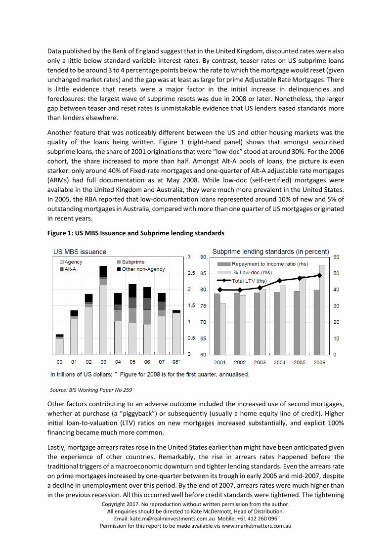
Another feature that was noticeably different between the US and other housing markets was the

quality of the loans being written. Figure 1 (right-hand panel) shows that amongst securitised

subprime loans, the share of 2001 originations that were “low-doc” stood at around 30%. For the 2006

cohort, the share increased to more than half. Amongst Alt-A pools of loans, the picture is even

starker: only around 40% of Fixed-rate mortgages and one-quarter of Alt-A adjustable rate mortgages

(ARMs) had full documentation as at May 2008. While low-doc (self-certified) mortgages were

available in the United Kingdom and Australia, they were much more prevalent in the United States.

In 2005, the RBA reported that low-documentation loans represented around 10% of new and 5% of

outstanding mortgages in Australia, compared with more than one quarter of US mortgages originated

in recent years.

Figure 1: US MBS Issuance and Subprime lending standards

Source: BIS Working Paper No 259

Other factors contributing to an adverse outcome included the increased use of second mortgages,

whether at purchase (a “piggyback”) or subsequently (usually a home equity line of credit). Higher

initial loan-to-valuation (LTV) ratios on new mortgages increased substantially, and explicit 100%

financing became much more common.

Lastly, mortgage arrears rates rose in the United States earlier than might have been anticipated given

the experience of other countries. Remarkably, the rise in arrears rates happened before the

traditional triggers of a macroeconomic downturn and tighter lending standards. Even the arrears rate

on prime mortgages increased by one-quarter between its trough in early 2005 and mid-2007, despite

a decline in unemployment over this period. By the end of 2007, arrears rates were much higher than

in the previous recession. All this occurred well before credit standards were tightened. The tightening



in credit, especially the reduced availability of subprime and Alt-A loans, was a response to increasing

delinquencies and defaults, not the initial impetus to them. This was exactly the opposite of the

sequence of events in other countries over the current cycle.

Full Recourse - incentive or deterrence

There are two competing motivations that drive mortgage delinquency and defaults. Whether a

lender chooses an ability-to-pay model or adopts the equity model which will determine if arrears are

a temporary setting or a permanent one. The equity model treats the choice to default as a put option.

It depicts borrowers as defaulting rationally when they are in negative equity. The concerns about

“walkaways” assume that this model describes household behaviour, or may increasingly come to do

so.

Evidence shows that allowing lenders recourse increases the likelihood that defaults will occur. This

may seem counter-intuitive, but when a lender is given the means to efficiently recover a debt by

seizure of the collateral, it does increase the probability of default. However, this same law can be an

important driver of the cultural mindset of a borrower. In Australia borrowers demonstrate a strong

resolve to maintain payments of their mortgage. Evidence suggests that Australian borrowers do

whatever they can not to default. They may get a second job, cut discretionary spending, or take their

children out of private school to save the home. Many analysts determine that this behaviour is driven

by recourse in Australia and compare this law of recourse to the US stereo type of “Jingle Mail” – when

a borrower sends the keys back to the bank and walks away from their debt. In Australia, the recourse

extends beyond the asset to the individual.

It is important to note that US mortgages in 23 of the 50 states is also with recourse. While it is true

that in many of these states the legislation is not as favourable to the lender as it is in Australia,

recourse beyond the home existed for many US mortgages. Further, it might be thought that housing

market risk differs between jurisdictions with full-recourse lending and those with non-recourse

lending. The experience of the US, indicates that the risk may be more similar than is commonly

thought. This is largely because, even in ostensibly full-recourse jurisdictions, it is quite practical for a

borrower to walk away from their debt. In Australia, ultimately this might require entering bankruptcy.

However, the stronger protection for lenders here in Australia does have a benefit in deterrence

against default, as demonstrated by the generally favourable credit outcomes of Australian borrowers.

The US system allows lenders to repossess the property faster than in other countries, which has

produced a different trade-off between speed and full asset recovery than elsewhere. As a result,

when house prices are rising, many US lenders have incentives which are tilted more strongly in favour

of lending based on collateral rather than affordability. If it turns out that the borrower cannot afford

to repay the loan, the lender can access the collateral relatively quickly in at least half of all US states.

Taking this together with differences in consumer protection regulation of mortgage lending itself, it

is no surprise that a lending sector with a collateral-based business model developed in the United

States

Borrowers default somewhat frequently

It’s accepted that defaults will occur, which is why the need for a structure to protect senior bond

holders, much like a bank’s equity and tiered capital instruments protect senior bond holders and

depositors. Borrowers do not set out to default when they borrow, it’s not in their mindset, and no

matter how good a bank’s underwriting process is, to determines the long-term ability for a borrower

to repay the loan, one cannot forecast factors around personal relationship breakdown, a household



member withdrawing from the labour market due to illness or pregnancy or death, which for the most

part is what is driving delinquencies in a relatively mute economic setting.

However, what does drive an increase in the probability of missed payments is small business failure,

high indebtedness and financial over-commitment, a sudden loss of income resulting from losing or

changing jobs or a, loss of overtime. If a sharp increase in missed payments does arise the dominant

reason is loss of employment or long-term unemployment. This will then drive an imbalance in

demand and supply of the underlying collateral, and see that collateral underperform.

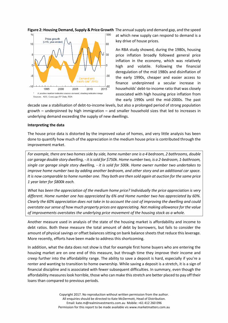
Specific groups that are more likely to miss payments are;

- Younger borrowers or a first home buyer, because LVRs are at their highest,

- Borrowers with dependent children, because they use the equity for private schooling or the Jones

affect and higher income or professional workers.

Research has shown that these same key factors to be to be significant drives of default— high

indebtedness (i.e. high loan-to-value ratio), age (young), households with dependent children and

higher than average incomes.

So, what are the buffers, to protect against house price demand and supply imbalances? The collateral

protection i.e. the physical house, is expressed as a Loan to Value (LVR) ratio. On average the LVR

across the securitised pools is circa 70% and for banks it’s as low as 55%.

Why do houses prices go up?

There are a variety of models and literature written about Australian House prices, much is focused

on the present state of prices, and are they in line with fundamental determinants, with some focusing

solely on supply or demand drivers independently to explain the growth.

The price of any good or asset is determined jointly by demand and supply contributions, and the price

today reflects what the buyer and seller are willing to accept as a reflection of the sum of expected

future discounted cash flows.

RBA research confirms that demand is driven from both owner occupiers and investors. It is affected

by considerations associated with, user cost (the rent vs own decision), and positively related to rent.

Other variables also play a role, like demographic factors, permeance of household income and the

cost of credit. Both owners and investors see the user cost as a measure of real interest rates, running

costs, maintenance and the expected real rate of house price appreciation. Additionally, an investor

would consider whether rental income would cover these user costs, after adjusting for tax

concessions.

Other macro factors like inflation affect house prices during various cycles like during the 1980s and

vice versa, disinflation, deregulation can also play a role.

The price of a house will behave differently to other assets because of the large transaction costs,

relatively thin market and heterogeneous environment. Demand will change faster than supply and

the price will need to adjust temporarily, unless vacant housing can absorb the change in demand.

Supply takes longer to adjust, due to the lead time to create new stock i.e. construction.



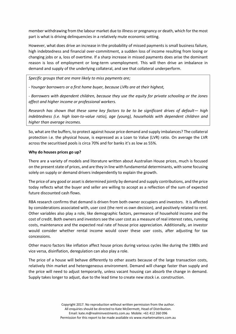
Figure 2: Housing Demand, Supply & Price Growth The annual supply and demand gap, and the speed

at which new supply can respond to demand is a

key drive of house prices.

An RBA study showed, during the 1980s, housing

price inflation broadly followed general price

inflation in the economy, which was relatively

high and volatile. Following the financial

deregulation of the mid 1980s and disinflation of

the early 1990s, cheaper and easier access to

finance underpinned a secular increase in

households’ debt-to-income ratio that was closely

associated with high housing price inflation from

the early 1990s until the mid-2000s. The past

decade saw a stabilisation of debt-to-income levels, but also a prolonged period of strong population

growth – underpinned by high immigration – and smaller household sizes that led to increases in

underlying demand exceeding the supply of new dwellings.

Interpreting the data

The house price data is distorted by the improved value of homes, and very little analysis has been

done to quantify how much of the appreciation in the medium house price is contributed through the

improvement market.

For example, there are two homes side by side, home number one is a 4 bedroom, 2 bathrooms, double

car garage double story dwelling, - it is sold for $750k. Home number two, is a 2-bedroom, 1-bathroom,

single car garage single story dwelling, - it is sold for 500k. Home owner number two undertakes to

improve home number two by adding another bedroom, and other story and an additional car space.

It is now comparable to home number one. They both are then sold again at auction for the same price

1 year later for $800k each.

What has been the appreciation of the medium home price? Individually the price appreciation is very

different. Home number one has appreciated by 6% and Home number two has appreciated by 60%.

Clearly the 60% appreciation does not take in to account the cost of improving the dwelling and could

overstate our sense of how much property prices are appreciating. Not making allowance for the value

of improvements overstates the underlying price movement of the housing stock as a whole.

Another measure used in analysis of the state of the housing market is affordability and income to

debt ratios. Both these measure the total amount of debt by borrowers, but fails to consider the

amount of physical savings or offset balances sitting on bank balance sheets that reduce this leverage.

More recently, efforts have been made to address this shortcoming.

In addition, what the data does not show is that for example first home buyers who are entering the

housing market are on one end of this measure, but through time they improve their income and

creep further into the affordability range. The ability to save a deposit is hard, especially if you’re a

renter and wanting to transition to home ownership. While saving a deposit is a stretch, it is a sign of

financial discipline and is associated with fewer subsequent difficulties. In summary, even though the

affordability measures look horrible, those who can make this stretch are better placed to pay off their

loans than compared to previous periods.



Property Crashes are not the same

In thinking about the RMBS market, investors should not confuse a fall in property prices with the

inability for a borrower to repay their loan. Hence, as RMBS investors, we are not specifically

concerned about house price volatility. We are concerned about the cyclical events that affect the

repayment ability of borrowers as these lead to the possibility of default. Large scale defaults will

impact house prices due to a large amount of properties being sold at one time, this is a simple law of

demand and supply. We will talk more about house price volatility later.

Many analysts look at the US property market and try to utilise that episode as a probable event here

in Australia. A major and profound feature of the housing crisis in the US was its speed, leading to a

cliff effect. The reality is that the crash in house prices was accelerated due to mass amounts of fraud,

bank intermediation failure and inferior product design. Using this as a comparison is not particularly

valid for forecast purposes because Australia just does not have the ingredients of mass fraud, bank

failure and inferior product design that prevailed in the US at the time.

The depth of price declines will always be a function within the localised markets of demand and

supply. The evidence in the US shows that, in the states where house prices fell the most (circa 70%),

there was mass over supply driven cheap credit and abundant products designed to suit speculators.

In the states where supply was not a major contributor, prices were only down 10% to 15%, akin to a

normal cyclical downturn in prices.

Property Crashes need a catalyst

The elements of a property crash include: supply exceeding demand; increasing fear that funding

conditions will tighten rapidly; and/or unemployment will rise sharply. These, collectively, will drive

the speed of the decline in house prices.

Analysis suggests that while short term factors have pushed median dwelling prices for Sydney and

Melbourne above their long-term equilibrium prices by about 14 percent and 8 percent respectively

(as at the end of FY2016), this degree of disequilibrium has been experienced previously in these

housing markets and they have managed to return to equilibrium without price movements

resembling a ‘bursting of the bubble’. Figure 2 over the page shows this in greater clarity.

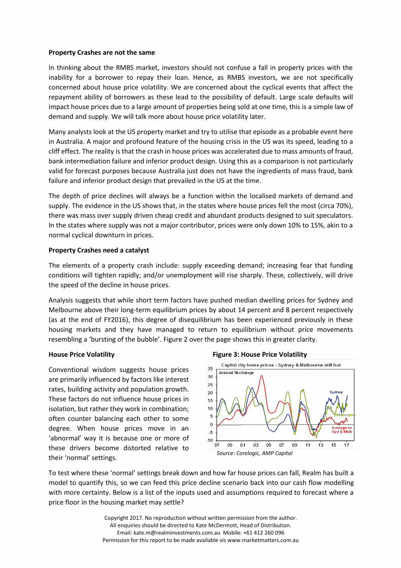
House Price Volatility

Conventional wisdom suggests house prices

are primarily influenced by factors like interest

rates, building activity and population growth.

These factors do not influence house prices in

isolation, but rather they work in combination;

often counter balancing each other to some

degree. When house prices move in an

‘abnormal’ way it is because one or more of

these drivers become distorted relative to

their ‘normal’ settings.

Figure 3: House Price Volatility

Source: Corelogic, AMP Capital

To test where these ‘normal’ settings break down and how far house prices can fall, Realm has built a

model to quantify this, so we can feed this price decline scenario back into our cash flow modelling

with more certainty. Below is a list of the inputs used and assumptions required to forecast where a

price floor in the housing market may settle?



Our analysis shows, as at Sep 2017, the forecast for the medium house price, is an expected 51%

decline from the current medium Australian House price of $670k.

Is there a floor in Property Prices in an Economic Depression?

We can observe that a significant move in property prices below the equilibrium in a downturn

scenario would require supply to exceed demand by approximately 46k units per month of stock (as

at Sep 2017). This scenario also assumes the ingredients for a cliff event are not present, an

unemployment rate of 25%, and credit condition to tighten significantly, driven by a sequence of

events that resemble the traditional triggers of a macroeconomic downturn.

A demand side response is assumed to occur from the latent demand in the economy driven by the

increased return or capitalisation rate for housing.

Figure 4: Realm House Price equilibrium model – Price Floor

The model forecasts the floor in

Property Prices and most

importantly the tipping point of the

system to where total system

failure occurs, and forbearance is

imposed. This is where the amount

of latent demand is overwhelmed,

and the banking system can no

longer foreclose and sell property

to the street.

See our paper ‘The Elasticity of

Arrears’ May 2012

Under the scenario of 25% unemployment, increased cap rate to 6%, and a significant cut to bank

lending, it forecasts a 45% price fall from the current level. The model has no context of time, but simply

predicts the clearing price level for Demand and Supply to come back to in equilibrium.

Figure 4 - Realm – House Price Model Imperial Assumptions

• Unemployment rate

• Size of Property Market

• Current House Price

• Amount of encumbered Property

• Bank Intermediation Assumption

• Eligible Borrowers

• Capitalisation Rate

Whilst protective of the details, we would be pleased to discuss the general workings of this model in

more depth if interested.



It’s just the Maths

Ratings agency opinions are influential. Unsurprisingly, there is a strong propensity for issuers to

manipulate the mortgage pools and tranche composition for best effect. To overcome these efforts,

we believe that using a Transition to Default Model approach rather than simple cash flow default

model is effective.

The standardised rating model gives an assessment of Loss Given Default for every loan in the pool for

a given LVR & borrower type in a great depression type event. In trying to model this scenario with

disaggregated data you can simply equate the Unemployment rate as the amount of loans that go into

arrears and subsequently default. This has merit if one can assume that the pool is representative of

the average borrower. For example, a 15% unemployment rate can imply that 15% of the pool would

default, this is harsh as, we have approximately 5% unemployment rate now, are 5% of mortgagees

defaulting? There is clearly a transition to a high number of defaults, so using an approximation as a

worse case based on a 1 for 1 delta is acceptable. So, let’s call this the Stressed Unemployment Rate

(SUmR).

One can also approximate House Price declines in a pool as to what potentially could occur at a system

level.

A simple formula can be applied to model the credit exposure of mortgage pools to demonstrate the

underlying intent of the structuring:

( (1 − 𝐴𝐿𝑉𝑅𝑃) − 𝐻𝑃𝐷 ) ∗ 𝑆𝑈𝑚R

where

ALVRP = Average LVR of the Pool

HPD = House Price Declines

SUmR = Stressed Unemployment Rate

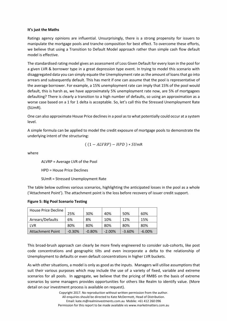
The table below outlines various scenarios, highlighting the anticipated losses in the pool as a whole

(‘Attachment Point’). The attachment point is the loss before recovery of issuer credit support.

Figure 5: Big Pool Scenario Testing

House Price Decline 25% 30% 40% 50% 60%

Arrears/Defaults 6% 8% 10% 12% 15%

LVR 80% 80% 80% 80% 80%

Attachment Point -0.30% -0.80% -2.00% -3.60% -6.00%

This broad-brush approach can clearly be more finely engineered to consider sub-cohorts, like post

code concentrations and geographic tilts and even incorporate a delta to the relationship of

Unemployment to defaults or even default concentrations in higher LVR buckets.

As with other situations, a model is only as good as the inputs. Managers will utilise assumptions that

suit their various purposes which may include the use of a variety of fixed, variable and extreme

scenarios for all pools. In aggregate, we believe that the pricing of RMBS on the basis of extreme

scenarios by some managers provides opportunities for others like Realm to identify value. (More

detail on our investment process is available on request).



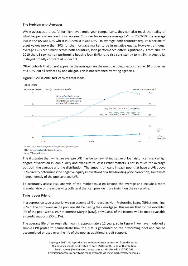
The Problem with Averages

While averages are useful for high-level, multi-year comparisons, they can also mask the reality of

what happens when conditions worsen. Consider for example average LVR. In 2009-10, the average

LVR in the US was 69% whilst in Australia it was 65%. On average, both countries require a decline of

asset values more than 30% for the mortgage market to be in negative equity. However, although

average LVRs are similar across both countries, loan performance differs significantly. From 2008 to

2010 the US saw its non-performing housing loan (NPL) ratio rise consistently to hit 8%; in Australia,

it stayed broadly constant at under 1%.

Other cohorts that do not appear in the averages are the multiple obligor exposures i.e. 10 properties

at a 50% LVR all services by one obligor. This is not screened by rating agencies.

Figure 6: 2008-2010 NPL of % of total loans

This illustrates that, whilst an average LVR may be somewhat indicative of loan risk, it can mask a high

degree of variation in loan quality and exposure to losses What matters is not so much the average

but both the average and the distribution. The amount of loans in each pool that have a LVR above

90% directly determines the negative equity implications of a 10% housing price correction, somewhat

independently of the pool average LVR.

To accurately assess risk, analysis of the market must go beyond the average and include a more

granular view of the underlying collateral that can provide more insight on the risk profile.

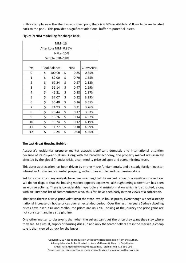
Time is your Friend

In a depression type scenario, we can assume 15% arrears i.e. Non-Preforming Loans (NPLs), meaning,

85% of the borrowers in the pool are still be paying their mortgage. This means that for the modelled

life of the pool, with a 1% Net Interest Margin (NIM), only 0.85% of the income will be made available

as credit support (85% x 1%).

The average life of an Australian loan is approximately 12 years, so in Figure 7 we have modelled a

simple CPR profile to demonstrate how the NIM is generated on the preforming pool and can be

accumulated or used over the life of the pool as additional credit support.



In this example, over the life of a securitised pool, there is 4.36% available NIM flows to be reallocated

back to the pool. This provides a significant additional buffer to potential losses.

Figure 7: NIM modelling for charge back

NIM= 1%

After Loss NIM= 0.85%

NPLs= 15%

Simple CPR= 18%

Yrs Pool Balance NIM Cum%NIM

0 $ 100.00 $ 0.85 0.85%

1 $ 82.00 $ 0.70 1.55%

2 $ 67.24 $ 0.57 2.12%

3 $ 55.14 $ 0.47 2.59%

4 $ 45.21 $ 0.38 2.97%

5 $ 37.07 $ 0.32 3.29%

6 $ 30.40 $ 0.26 3.55%

7 $ 24.93 $ 0.21 3.76%

8 $ 20.44 $ 0.17 3.93%

9 $ 16.76 $ 0.14 4.07%

10 $ 13.74 $ 0.12 4.19%

11 $ 11.27 $ 0.10 4.29%

12 $ 9.24 $ 0.08 4.36%

The Last Great Housing Bubble

Australia’s residential property market attracts significant domestic and international attention

because of its 25-year bull run. Along with the broader economy, the property market was scarcely

affected by the global financial crisis, a commodity price collapse and economic downturn.

This asset appreciation has been driven by strong micro fundamentals, and a steady foreign-investor

interest in Australian residential property, rather than simple credit expansion alone.

Yet for some time many analysts have been warning that the market is due for a significant correction.

We do not dispute that the housing market appears expensive, although timing a downturn has been

an elusive activity. There is considerable hyperbole and misinformation which is distributed, along

with an illustrious list of commentators who, thus far, have been early in their views of a correction.

The fact is there is always price volatility at the state level in house prices, even though we see a steady

national increase on house prices over an extended period. Over the last five years Sydney dwelling

prices have risen 73% and Melbourne prices are up 47%. Looking at the journey the price gains are

not consistent and in a straight line.

One other matter to observe is that when the sellers can’t get the price they want they stay where

they are. As a result, supply of housing dries up and only the forced sellers are in the market. A cheap

sale is then viewed as luck for the buyer!



There also a lot of granular data available around post codes and specific regions. This data shows,

further substantial local volatility. Housing markets are not homogeneous across Australia’s states and

territories. Housing markets are not even homogeneous within each state or territory, with market

dynamics different between capital cities, major towns and rural and regional locations.

Much applied economic research has focused on what are the primary drivers influencing house price

growth in Australia. KPMG Economics has found that an error-correction model to be a useful aid in

further understanding the behaviour of the Sydney and Melbourne housing markets. Using this

approach KPMG Economics found evidence of a long-run relationship between house prices and

variables relating to the stock of dwellings, population and borrowing by residential property

investors.

The surge in prices and debt has led many to conclude a crash is imminent. But we have heard that

many of times over the last 10-15 years. In 2004, The Economist magazine described Australia as

“America’s ugly sister” thanks in part to a “borrowing binge” and soaring property prices. Most

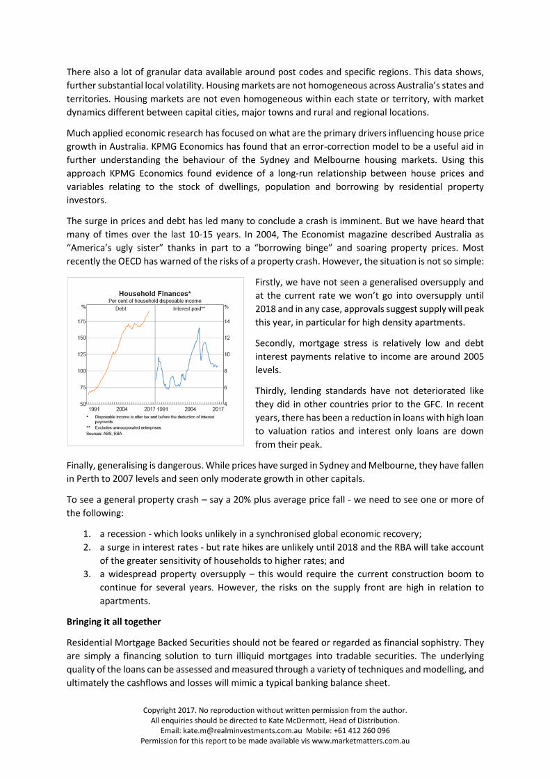
recently the OECD has warned of the risks of a property crash. However, the situation is not so simple:

Firstly, we have not seen a generalised oversupply and

at the current rate we won’t go into oversupply until

2018 and in any case, approvals suggest supply will peak

this year, in particular for high density apartments.

Secondly, mortgage stress is relatively low and debt

interest payments relative to income are around 2005

levels.

Thirdly, lending standards have not deteriorated like

they did in other countries prior to the GFC. In recent

years, there has been a reduction in loans with high loan

to valuation ratios and interest only loans are down

from their peak.

Finally, generalising is dangerous. While prices have surged in Sydney and Melbourne, they have fallen

in Perth to 2007 levels and seen only moderate growth in other capitals.

To see a general property crash – say a 20% plus average price fall - we need to see one or more of

the following:

1. a recession - which looks unlikely in a synchronised global economic recovery;

2. a surge in interest rates - but rate hikes are unlikely until 2018 and the RBA will take account

of the greater sensitivity of households to higher rates; and

3. a widespread property oversupply – this would require the current construction boom to

continue for several years. However, the risks on the supply front are high in relation to

apartments.

Bringing it all together

Residential Mortgage Backed Securities should not be feared or regarded as financial sophistry. They

are simply a financing solution to turn illiquid mortgages into tradable securities. The underlying

quality of the loans can be assessed and measured through a variety of techniques and modelling, and

ultimately the cashflows and losses will mimic a typical banking balance sheet.



The perception that all RMBS is bad, is predicated on the proximity to the recent US Subprime crisis

and, possibly, Hollywood dramatization. The facts are that RMBS, like corporate debt, are risk assets

that perform and underperform through economic cycles.

There needs to be certain out of cycle factors to drive defaults and losses like the US Subprime

experience. These factors include:

• a massive over supply of housing,

• deterioration of lending standards, and

• an element of wide scale fraud at the borrower level.

Australia’s mortgage market has some unique features which make it extremely hard for a cliff effect

in arrears and default, as occurred in the US, to take hold. For one, recourse in Australia acts more as

a deterrent to guide behaviour, rather than a credit enhancement feature as it is the US. House price

movements are not enough in isolation to create a destructive feedback cycle.

These observations have been the common thread of every major crisis over the last 200 years.

We Are Not RMBS Apologists!!

Investors should not confuse our deep understanding of this market with an attestation of undying

loyalty and devotion, in fact much the opposite. At the same time, we note that certain biases have

seemingly calcified within the markets perception which can present a challenge when seeking to

communicate our exposure to this sector. Indeed, we find it interesting that very often investors who

are accepting relatively shallow system risk (such as bank AT1) will express an aversion to the

structured credit universe.

Like any form of financial product or construct of financial engineering of RMBS structures are subject

to layering risk which is how issuers rent seek. We are skilful in identifying this and pricing for risk

appropriately. At the same time the vehicles do achieve their desired objective of transforming

heterogeneous risks into broad systematic or market risk, that is in essence very similar to other forms

of bank risk such as senior bank debt and in the case of mezzanine debt AT1 and T2 products.

As such our view around system will be reflected within our weighting to Australian systematic risk

more broadly be it AT1, T2 and indeed RMBS.

There are plenty of examples in history where clever ideas get pushed too far. This in many ways holds

true for Securitisation. A financing technique that is as old as banking itself, that functionally

recognises the benefit of diversity delivered by the law of large numbers. It’s the same mathematical

premise that underpins insurance, capacity of public infrastructure and any other mathematical

process where individual risks and behaviours are transformed into network wide or system wide

assumptions. This mathematical process was pushed to its absolute limit in the GFC through unbridled

greed and a lack of structure and accountability.

In this document we have covered off the idiosyncrasies that drove this. However, we also feel it’s

important to challenge the bias which now seems to be semi-permanent within investment markets,

where the RMBS acronym has almost become an anathema.



Who are Realm Investment House

Realm Investment House (Realm) is a fixed income specialist with a low risk approach to high yield

investing. The Realm Investment Team (Team) believe that capital preservation, regular income and

low volatility can be achieved by a risk first approach when investing in fixed income.

Realm’s flagship strategy, the Realm High Income Fund (Fund) aims to provide regular income of 3%

(net of fees and after franking) over the RBA cash rate through the market cycle, while seeking to

preserve capital. To achieve this the Fund invests primarily in domestic investment grade asset

backed securities and corporate bonds, as well as government bonds and hybrids. The team actively

manage the credit exposures to mitigate risk and manage the portfolio as a full sector, relative value,

absolute return strategy. For further information on the Realm High Income Fund Click Here.

Realm Capital Series Fund – The Team believes high yield investing has a key role in portfolios and

that there are good times to allocate to these opportunities and not so good times. Offering a high

yield fund open to investor applications and redemptions regularly, in our opinion, is a flawed

structure. Volatility does not care how good your portfolio is. It will reprice it basis where market

liquidity is, which will create volatility in returns. This spooks investors and may cause them to “run

for the door”, meaning that at the very time the manager should be allocating into credit

opportunities, they are in fact liquidating them to fund these withdrawals.

The Team feel to extract the full value of credit opportunities the correct structure is one where

investors and the manager can agree to an investment timeframe. To provide non-institutional

investors such opportunities the Team have created an unlisted investment offering via the Realm

Capital Series Fund.

The first opportunity within the series is the Realm Capital Series 2018-1 Units, allocating into

Residential Mortgage Backed Securities (RMBS) capital markets, focusing on bank warehouse funding.

The Team believe the benefit of short term exposures vs the term funding markets, the return

premium for low liquidity and high complexity plus the corporate credit guarantees underpinning

these structures represent significant relative value versus the opportunities in the general RMBS term

securities market.

The Realm Capital Series 2018-1 Units will target a return of 6.25%, variable for 5 years and linked to

the cash rate. For more information regarding this offer please contact your adviser.

Disclaimer

Confidentiality Notice: This e-mail is confidential and may also be legally privileged. If you are not the

intended recipient you may not copy, forward, distribute, disclose or use any part of it. If you have

received this message in error, please delete it and all copies from your system and notify the sender

as soon as possible by return e-mail. We do not guarantee the integrity of any e-mails or attached files

and are not responsible for any changes made to them by any other person.

General Advice Warning: Realm Pty Ltd AFSL 421336. Please note that any advice given by Realm Pty

Ltd and its authorised representatives is deemed to be GENERAL advice, as the information or advice

given does not take into account your particular objectives, financial situation or needs. Therefore, at

all times you should consider the appropriateness of the advice before you act further. Further, our

AFSL only authorises us to give general advice to WHOLESALE investors.

http://www.realminvestments.com.au/high-income-fund.shtml

demystifying australian residential mortgage backed … · banks fund thousands of loans like an...

Documents