Accepted to Combustion and Flame Feb. 11, 2004

Demonstration of a Free-Piston Rapid Compression Facility for the Study of High Temperature Combustion Phenomena

M. T. Donovan, X. He, B. T. Zigler, T. R. Palmer, M. S. Wooldridge, and A. Atreya

Department of Mechanical Engineering University of Michigan

2350 Hayward St. Ann Arbor, MI, USA 48109-2125

Abstract

A free-piston rapid-compression facility (RCF) has been developed at the University of

Michigan (UM) for use in studying high-temperature combustion phenomena, including gas-

phase combustion synthesis and homogeneous charge compression ignition systems. The facility

is designed to rapidly compress a mixture of test gases in a nearly adiabatic process. A range of

compression ratios, currently 16 to 37, can be obtained. The high temperatures and pressures

generated by the RCF can be maintained for in excess of 50 ms, providing an order of magnitude

increase in observation time over what can be obtained using shock tubes. The facility is

instrumented for temperature and pressure measurements as well as optical access for use with

laser and other optical diagnostics. This work describes the UM-RCF and its operation,

establishes obtainable pressures and temperatures (over 1900 kPa and 970 K for predominately

N2 gas mixtures, and over 785 kPa and 2000 K for Ar gas mixtures), and demonstrates the

repeatability of the UM-RCF experiments (< 3% run-to-run variability in peak pressure) for

combustion studies. The experimental results for time histories of temperature and pressure are

interpreted using analytical isentropic models. Comparison between the isentropic predictions

and the experimental data indicate excellent agreement and support the conclusion that the core

region of the test gases is nominally uniform and is compressed isentropically.

2

1. Introduction

The study of complex combustion chemistry requires experimental facilities that can replicate

combustion environments of interest. Chemical kinetics can have considerable impact on

characteristics important in many combustion systems. For example, ignition delay and particle

nucleation can have long characteristic times [1] that are dominated by reaction kinetics [2]. In

both these systems, the study of the chemical kinetics is fundamental to the overall

understanding of the respective combustion processes.

Ignition studies are of considerable importance in the development of advanced internal

combustion engine strategies. Of particular interest are homogenous charge compression

ignition (HCCI) systems as these engines are compression ignited, lean burn, and have no

throttling losses, which leads to high efficiency and low NOx emissions [3]. In HCCI engines,

combustion is achieved through control of the temperature, pressure, and composition of the

reactant mixture, and extensive understanding of the chemical kinetics of ignition is required to

develop control strategies.

The process of particle nucleation (the formation of particles < 5-10 nm in size) is the

least understood step in particle formation and growth in combustion systems [4]. The ability to

control the creation and growth of particles is critical to minimize, or ideally eliminate,

particulate pollution. Additionally, increased understanding of particle nucleation can be used to

design and create nano-particles at the molecular level.

Desirable characteristics for an experimental combustion chemistry facility to study

relatively long time combustion phenomena include high temperatures (and pressures), simple

flow fields, good measurement access, and sufficient test times to examine the phenomena of

interest. Existing experimental tools have some of these characteristics. Shock tubes generate

3

high temperatures without complicated flow dynamics and are ideal for the study of combustion

phenomena with fast characteristic times. However, the uniform elevated temperature and

pressure post-shock conditions typically persist for less than 5 ms [5]. On the other hand, a rapid

compression facility (RCF) is capable of generating high temperatures and pressures, with

simplified fluid mechanics, for sustained periods (greater than 10 ms).

In its most basic form, the RCF can be described as a simple piston-cylinder device. An

external force (usually a compressed gas or a pressurized liquid) is used to rapidly accelerate the

piston within the cylinder. The piston compresses the test gas mixture in the cylinder, much like

the compression stroke of an internal combustion (IC) engine, leading to a very rapid increase in

pressure and temperature. By preventing piston rebound, the high pressure and temperature

conditions can be sustained for a relatively long duration (>10 ms). Due to the speed of the

compression process, there is little time for heat transfer and the bulk of the test gas mixture is

thermally isolated from the RCF (i.e. cooling due to heat transfer is restricted to a thin layer of

gases along the bounding surfaces of the RCF). The effect of limited heat transfer is that

conditions (temperature, pressure, and species concentration) within a core region of the

compression mixture are (nominally) spatially uniform.

Various researchers have used rapid-compression facilities for generating high pressure

and temperature conditions. Investigations using RCFs have focused primarily on ignition delay,

auto-ignition and two-stage ignition phenomena.

Griffiths and co-workers at Leeds University have used a pneumatically driven piston for

autoignition studies [6,7] of hydrocarbon fuels and the investigation of single and two-stage

ignition of alkanes [8]. In support of their experimental work, this group studied the

development of the temperature field [9], performed computational fluid dynamics (CFD)

4

modeling [10], and performed extensive kinetics modeling of reaction chemistry [11, 2].

Recently, the Leeds research group has studied the thermokinetic interactions that lead to knock

in HCCI using image intensified, natural light output to characterize the reaction [12]. The

Leeds RCF achieves compression ratios up to 14.6. Compression occurs in 22 ms, and final

temperatures of 530 to 1000 K and pressures up to 2000 kPa are realized.

Minetti and co-workers, at the University of Science and Technology (UST) at Lille, used

an RCF to study auto-ignition [13] and two-stage ignition [14, 15, 16] of hydrocarbon fuels. In

support of their experimental work, this group investigated the temperature distribution within

their RCF [17, 18] and conducted kinetic modeling of their RCF experiments [13, 19]. The UST

RCF system uses a dual piston design: an air-driven drive piston is connected, by way of a cam,

to a second piston that compresses the test gas mixture. The design of the cam controls the

stroke of the compressing piston and prevents rebound of the compressing piston when it reaches

full extension. The UST RCF is capable of achieving a compression ratio of approximately 10.

Final pressures of up to 1700 kPa and temperatures of 900 K have been reported with

compression times of 20 to 60 ms using this facility.

Lee and Hochgreb at the Massachusetts Institute of Technology (MIT) used an air driven,

oil damped RCF piston system [20] to study hydrogen auto-ignition [21]. Lee and Hochgreb

have performed detailed modeling of the suppression of vortices, which are formed by the piston

in this facility during compression, and the heat transfer that occurs within the MIT RCF [22].

This modeling work led to modifications to their piston design to capture the vortices created

during the compression process and hence reduce fluid motion, and the subsequent heat transfer,

in the test gas. More recently, Tanaka and co-workers have used this RCF to study the effects of

fuel structure and additives on HCCI combustion [23, 24]. The maximum pressure, compression

5

ratio, and temperature achieved using the MIT device were 7 MPa, 19, and 1200 K, respectively.

Compression in 10 to 30 ms was reported.

Researchers at the National University of Ireland (NUI), Galway used an RCF to study

methane and propane ignition [25, 26]. The NUI RCF is a novel design that incorporates

opposed pistons to rapidly compress a test gas mixture [27]. Compression ratios as high as 13.4

have been reported using this RCF and peak compression pressures and temperatures of 4 MPa

and 1060 K, respectively, have been reported. The compression time using this RCF is less than

20 ms.

As demonstrated by the results of other researchers using RCFs, the sustained high

temperature and pressure environment created by an RCF provide an excellent research tool for

simulating adiabatic compression and ignition. These conditions also happen to be well suited to

the study of particle nucleation phenomena. The extended duration high temperature

environment permits the monitoring of chemical reactions as they evolve over time. The

simplified fluid mechanics found in RCFs permit rather straightforward determination of the

combustion conditions. The good measurement access afforded by RCFs also allows for the use

of a wide range of optical and physical diagnostics.

A free-piston rapid-compression machine, originally designed by TRW to study sooting

in hydrocarbon flames [28], has been relocated to the Department of Mechanical Engineering at

the University of Michigan (UM). The RCF has been installed and refurbished for use in

studying high-temperature combustion phenomena. Prior to using the UM-RCF for combustion

studies, the performance of the device must be characterized with benchmarking experiments.

To properly characterize performance, it is necessary to demonstrate the UM-RCF generates test

conditions conducive to the study of a range of combustion phenomena. Furthermore, these test

6

conditions should be both repeatable and predictable. The current work describes the UM-RCF

and its operation, and presents the results of characterization studies of the UM-RCF, including

analytical models developed to predict the performance of the RCF over a range of operating

conditions. The results of the benchmark experiments will confirm the ability of the RCF to

repeatably achieve sustained high-temperature and high-pressure operating conditions.

2. Experimental Facility

Hardware and Instrumentation

A schematic and photograph of the UM-RCF are shown in Fig. 1. The key components of the

UM-RCF are the driver section, the driven section, the test manifold, the sabot (free-piston), and

the hydraulic control valve assembly. The UM-RCF uses pressurized gas to accelerate the sabot

down the bore of the driven section. The test gases are loaded into the driven section, in front of

the sabot, and are compressed as the sabot traverses the length of the driven section. The sabot

lodges in the test manifold, confining a portion of the compressed gases within the test manifold

of the UM-RCF.

The driver section is a 5.54 m long carbon steel pipe with a 154 mm inner diameter. The

section is capped on one end and separated from the driven section on the other end by a

101.6 mm diameter globe valve. The driver section acts as a reservoir for the pressured gas

(typically air) used to propel the sabot during a UM-RCF experiment.

The driven section is a 2.74 m long stainless steel tube. The inner surface is chromed and

honed to a diameter of 101.2 mm. The driven section is connected to the globe valve at one end

and the test manifold at the other end. Test gases mixtures are loaded into the driven section

prior to operating the UM-RCF and the driven section acts as the cylinder through which the

sabot travels during operation of the UM-RCF.

7

The test manifold consists of four components: the convergent section, the extension

section, the thermocouple manifold, and the instrumented test section. The stainless steel

convergent section is 101.6 mm long and bridges the 101.2 mm bore of the driven section with

the 50.8 mm bore of the remainder of the test manifold components. The extension section is a

stainless steel tube (50.8 mm bore) that provides the contact surface used to halt the motion of

the sabot. Two sections are available for use (81 mm or 126 mm in length), which allow for

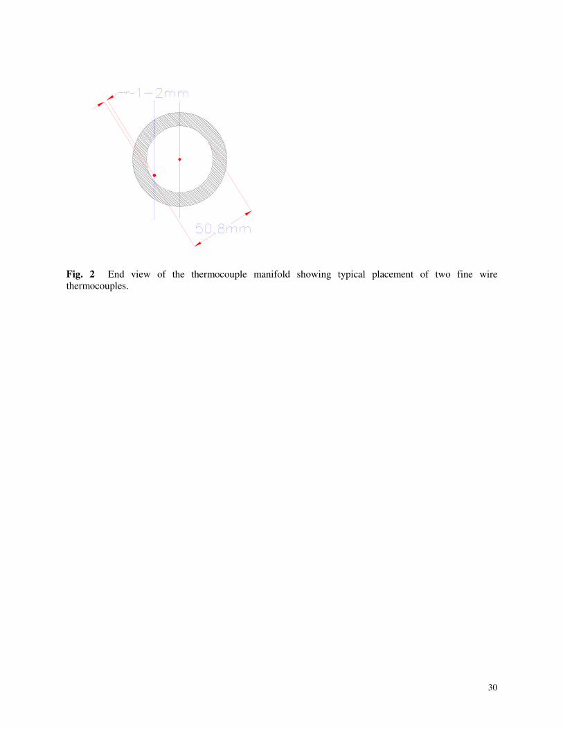
control of the overall compression ratio of the UM-RCF. The polycarbonate thermocouple

manifold is designed for the mounting of fine wire thermocouples across the bore of the test

manifold (see Fig. 2). Like the other components in the test manifold, the thermocouple

manifold has a bore of 50.8 mm. The length of the thermocouple manifold varies by design and

is either 16.2 or 25.4 mm long, which alloys for further control of the overall compression ratio

of the UM-RCF. This component is optional and can be removed for experiments where

temperature measurements are either unnecessary or conditions are unsuitable for the use of fine

wire thermocouples.

The instrumented test section, depicted in Fig. 3, contains two optical ports (for use with

optical diagnostics), a pressure transducer port, an additional instrumentation port and a gas

inlet/outlet port. The test section has a length of 50.8 mm. An end wall seals the test manifold.

Typically, the end wall is a 6.3 mm thick steel plate, although it can be replaced with at 12.7 mm

thick polycarbonate plate that permits additional optical access to the test manifold. A third

option involves replacing the end wall with a fast acting valve connected to an evacuated

expansion tank. The valve and expansion tank can be used to rapidly quench the gases in the test

volume, permitting the “freezing” of test conditions at a pre-selected time after the completion of

compression.

8

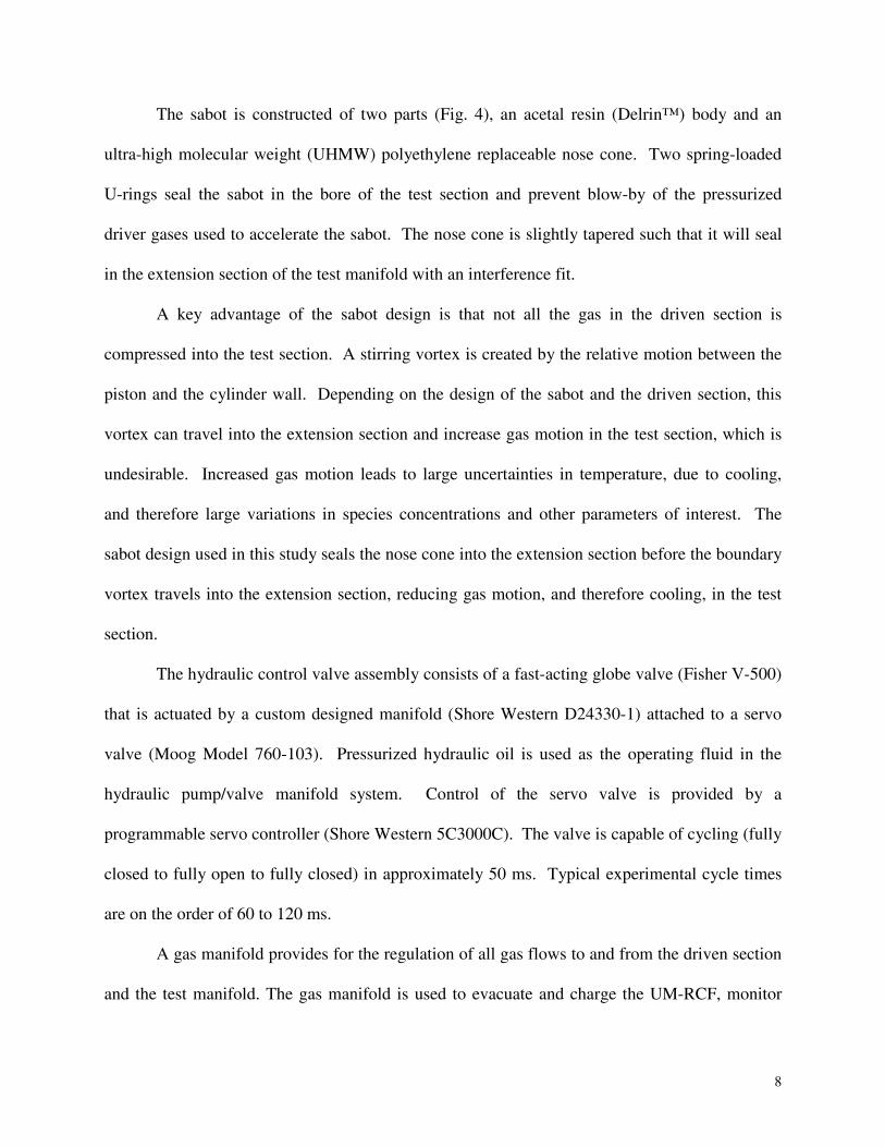
The sabot is constructed of two parts (Fig. 4), an acetal resin (Delrin™) body and an

ultra-high molecular weight (UHMW) polyethylene replaceable nose cone. Two spring-loaded

U-rings seal the sabot in the bore of the test section and prevent blow-by of the pressurized

driver gases used to accelerate the sabot. The nose cone is slightly tapered such that it will seal

in the extension section of the test manifold with an interference fit.

A key advantage of the sabot design is that not all the gas in the driven section is

compressed into the test section. A stirring vortex is created by the relative motion between the

piston and the cylinder wall. Depending on the design of the sabot and the driven section, this

vortex can travel into the extension section and increase gas motion in the test section, which is

undesirable. Increased gas motion leads to large uncertainties in temperature, due to cooling,

and therefore large variations in species concentrations and other parameters of interest. The

sabot design used in this study seals the nose cone into the extension section before the boundary

vortex travels into the extension section, reducing gas motion, and therefore cooling, in the test

section.

The hydraulic control valve assembly consists of a fast-acting globe valve (Fisher V-500)

that is actuated by a custom designed manifold (Shore Western D24330-1) attached to a servo

valve (Moog Model 760-103). Pressurized hydraulic oil is used as the operating fluid in the

hydraulic pump/valve manifold system. Control of the servo valve is provided by a

programmable servo controller (Shore Western 5C3000C). The valve is capable of cycling (fully

closed to fully open to fully closed) in approximately 50 ms. Typical experimental cycle times

are on the order of 60 to 120 ms.

A gas manifold provides for the regulation of all gas flows to and from the driven section

and the test manifold. The gas manifold is used to evacuate and charge the UM-RCF, monitor

9

pressures within the UM-RCF during charging and evacuation and to prepare test gas mixtures.

Test gas mixtures are typically prepared in a mixing tank. The test gas mixture composition is

determined by measurement of the partial pressures of the various gas components using three

capacitance manometers (Varian models VCMT11T, VCMT12T, and VCMT13T) with 1.3 kPa,

13.3 kPa, and 133 kPa maximum scales, and a Bourdon tube gauge (Omega DPG5000-L) with a

maximum scale of 410 kPa.

The following diagnostics are installed in the test manifold of the UM-RCF. A

piezoelectric transducer (Kistler 6041AX4 with Type 5010B charge amplifier) is used to record

dynamic pressures during the test period (<10 µs time response and dynamic range of 0 to

5000 kPa). A thermal isolation coating (RTV) on the pressure transducer was used in some

experiments to test the influence of thermal shock. (The results indicated that thermal shock had

no effect on the performance of the transducer.) Temperatures during the test period are

recorded using uncoated 0.025 mm diameter (~0.080 mm bead diameter) S-type (Pt/Pt-10%Rh)

thermocouples (Omega Engineering, P10R-001). Typically, two thermocouples are installed in

the temperature measurement section. One thermocouple bead is located nominally in the center

of the chamber (25.4 mm from the wall) and the second thermocouple bead is located near the

wall of the thermocouple manifold (within 2 mm, see Fig. 2). Typical performance

characteristics of the thermocouples are discussed below. The sabot position measurement

system consists of a pair of diode lasers (TIM-201-3, 3 mW, 650 nm) and unamplified silicon

photo-detectors (Hamamatsu S1787-12, 3 dB response time < 10 ms) that record the location of

the sabot near the end of its travel (see Fig. 1). Passage of the sabot interrupts the laser beams,

recording the location of the sabot within the driven section. The sabot position within the

driven section is used to develop volume time-histories of the test gas for use in computational

10

modeling of the compression process. Optical ports in the test section provide access for both

absorption and emission spectroscopy. Data are recorded using a high-resolution digital data

acquisition system (National Instruments PXI NI4472 data acquisition board) with a sampling

rate of 100 kHz and 24-bit resolution. Simultaneous data acquisition is provided by a high-speed

four channel digital oscilloscope (HP Infinium 54845).

Operation

Operation of the UM-RCF begins with loading the sabot into the driven section just downstream

of the globe valve (which is in the closed position). All connections are secured and the device

is leak tested. Typical leak rates of the combined driven section and test manifold are < 2 Pa

(0.015 torr) per minute. The driven section is evacuated to below 400 Pa (3 torr) and purged

with an inert gas (N2 or Ar). After three purges, the driven section is evacuated to below 35 Pa

(0.25 torr) and charged with the test gas mixture. Typically test gas mixtures are prepared in

advance and stored in a dedicated mixing tank. Initial test gas pressures range from 2.5 to

30 kPa (20 to 220 torr). All test gases used in this study have a purity of at least 99.998%

(except O2 which has a purity of at least 99.98%).

Once the test mixture has been loaded into the driven section, all isolation valves are

closed, the data acquisition equipment is readied, and the driver section is pressurized with air

(103 to 290 kPa). The globe valve is then rapidly cycled using the servo controller. The

pressurized gas from the driver section accelerates the sabot down the length of the driven

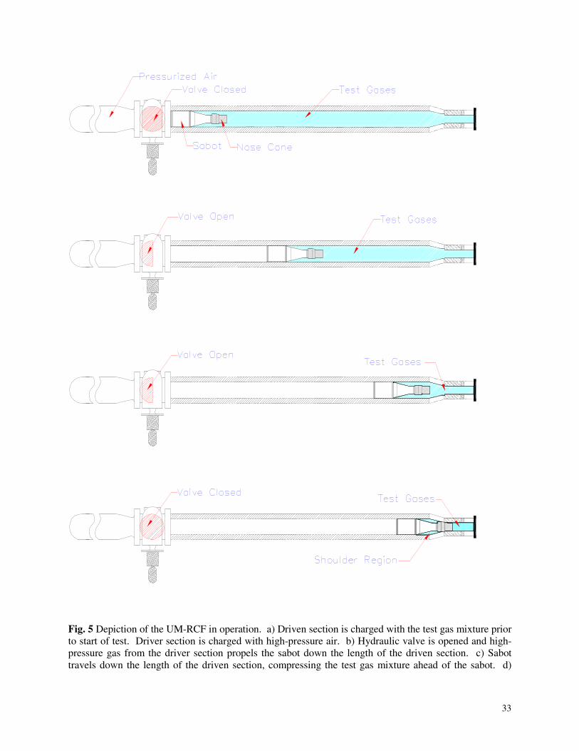
section, rapidly compressing the test gas mixture into the test manifold. The compression

process is depicted in Fig. 5 as a series of four drawings that show the sabot as it compresses the

test gas mixture within the UM-RCF. The sabot motions stops when the nose cone of the sabot

lodges in the extension section. (The sabot body typically separates from the nose cone at this

11

point, rebounds, and comes to rest within the driven section.) The terminal velocity of the sabot

ranges from 20 to 40 m/s. The lodging of the nose cone seals the test section from the driver

section gases and prevents rebound of the nose cone and out-leakage of the test gases. The

experimental data are recorded before, during and after the compression process.

Distinct UM-RCF Design Features

Several design features of the UM-RCF serve to distinguish the device from other rapid-

compression facilities. These features include the large range of compression ratios that can be

obtained, the novel sabot design that minimizes fluid disturbances in the test volume, the ability

to make temperature measurements at multiple locations within the test volume, and good optical

access (see Fig. 3).

The UM-RCF has three elements that can be adjusted to modify the compression ratio.

Two extension sections (81 mm and 126 mm long) can be used (alone or in series) to change the

length of the test volume. Two thermocouple sections (16 and 25.4 mm long) can also be used to

modify the test volume. Lastly, the length of the nose cone can be adjusted (from 38 to 89 mm)

to control how far the nose cone enters the test volume. The combination of these three elements

permits the UM-RCF to achieve volumetric compression ratios from 16 to 37.

The design of the sabot is a slight modification (incorporating a change in materials and

improvements to sabot balance) of the original TRW design [28] used during their operation of

the UM-RCF in the late 1980s. A key feature of the design is the sloped portion of the sabot

base (see Figs. 4 and 5). As the sabot travels down the barrel, the motion of the sabot, relative to

the walls of the driven section, creates fluid disturbances. In a traditional piston-cylinder

arrangement, these fluid disturbances will act to greatly enhance heat transfer in the test volume

and drastically reduce the time at which high-temperature combustion conditions can be

12

maintained. As shown schematically in Fig. 5, most of the fluid disturbances are effectively

captured in the volume between the sloped face of the sabot base and the converging section of

the UM-RCF. This greatly reduces induced fluid motion in the test volume and increases the

time at which high-temperature conditions persist in the test volume.

The thermocouple manifold permits the simultaneous in situ measurement of gas

temperatures at multiple radial locations within the test volume (see Fig. 2). A pair of

thermocouple manifolds can be used simultaneously to measure temperature at different axial

locations within the test manifold. The ability to make temperature measurements throughout

the course of UM-RCF experiments is a valuable experimental tool. Other researchers have used

thermocouples to investigate the temperature field in RCFs [18], but these measurements were

obtained under limited conditions and were not available for the full duration of reactive

experiments (experiments were quenched prior to ignition). Temperature measurements have

also been obtained using Rayleigh scattering [9, 17, 18] and laser-induced fluorescence (LIF) [9].

To our knowledge, the use of thermocouples while operating at typical conditions, including

with reacting mixtures, is unique to the UM-RCF. Data from the thermocouple measurements

can be used to validate modeling of the compression process, provide accurate data on pre-

reaction conditions (temperature need not be inferred from ideal gas or isentropic relations), and

can help quantify temperature non-uniformities within the test volume.

Ports in the test section provide optical access to the test volume. This access can be used

for various optical diagnostics, including laser absorption spectroscopy, particle scattering, and

emission spectroscopy. The steel end wall of the test manifold can be replaced with a

polycarbonate window. This window provides excellent optical access to the test volume and

permits optical recording of experiments within the UM-RCF.

13

3. Results and Discussion

To demonstrate the ability of the UM-RCF to generate conditions suited to the study of a wide

range of combustion phenomena, a series of experiments were conducted using a mixture of N2

and O2, pure N2, and Ar as the test gases. In addition to demonstrating the range of test

conditions achievable within the UM-RCF, the benchmarking experiments will also show the

repeatability of conditions within the UM-RCF. The N2/O2 mixtures represent the bulk of the

gas constituents used in the study of combustion synthesis of SiO2 nanoparticles. The

experiments with N2 as a test gas are proxies for the conditions typical of hydrocarbon ignition.

The Ar mixtures generate test conditions that would be suited to the study of very high

temperature combustion phenomena and demonstrate the range of capabilities of the UM-RCF.

Non-reactive mixtures are used for all performance benchmark experiments for two reasons.

First, fundamental RCF performance is easier to quantify in the absence of chemical reaction.

Second, in the planned combustion experiments, reactants are only expected to make up a small

fraction of the test gas mixtures (mole fractions of <2 %). Ar, N2, and O2 are the bulk of the gas

constituents in the mixtures, and therefore the behavior of these gases will strongly determine the

behavior of the overall test gas mixtures.

Figure 6 presents a typical pressure/temperature time-history from an N2/O2 mixture

experiment in the UM-RCF. The initial pressure (Po) of the mixture in the driven section was

3.37 kPa (25.3 torr) and the mixture was 95.9% N2, on a mole basis, with the balance being O2.

The peak experimental temperature (Tmax) and pressure (Pmax) observed were 965 K and 219 kPa,

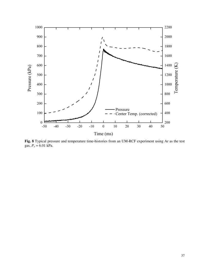
respectively. Figures 7 and 8 present similar pressure/temperature time-histories for experiments

with N2 (Po = 26.7 kPa, Tmax = 971 K, Pmax = 1940 kPa) and Ar (Po = 6.01 kPa, Tmax = 1996 K,

Pmax = 774 kPa) as the test gases. All experimental data in Figs. 6 to 8 have been filtered to

14

remove high frequency (>1 kHz) noise. Additionally, the temperature data have been processed

to account for the time response of the thermocouples and include corrections for radiation heat

transfer. The thermocouple data processing is discussed in further detail below. Included in

Fig. 6 are the raw pressure and temperature data obtained at the end of the compression event.

The raw data provide an indication of the typical level of disturbances observed in the data.

Several features are worth noting regarding Figs. 6 to 8:

• The bulk (80%) of the pressure rise and the majority (50%) of the temperature rise

occur in a very short time (<10 milliseconds). This quick compression minimizes the

cooling of the test gas mixture at the walls of the UM-RCF.

• The compression process occurs smoothly, without any significant pressure

disturbances prior to seating of the sabot in the extension section. The final impact of

the sabot into the test manifold does create some small pressure disturbances (see

inset figure of Fig. 6). As noted above, these high frequency (>1 kHz) disturbances

generated by the impact are filtered from the data. The source and magnitude of these

pressure disturbances are discussed in more detail below.

• Combustion conditions (pressure > 75% Pmax, temperature > 80% Tmax) are

maintained in the test manifold for approximately 50 ms or longer depending on the

test conditions and composition of the test gas mixture.

• Cooling of the test gases occurs gradually over time (as seen in the pressure data),

without any sharp changes that would indicate greatly enhanced heat transfer due to

large-scale fluid motion.

• Unsteadiness in the temperature trace (at long times, t > 20 ms) is primarily

attributable to motion of the thermocouple. The location of the thermocouple bead

15

fluctuates slightly within the test volume due to fluid motion and thermal expansion

of the thermocouple wires, leading to variation in the measured temperature. This

thermocouple motion has been observed via high speed imaging through the

transparent end wall.

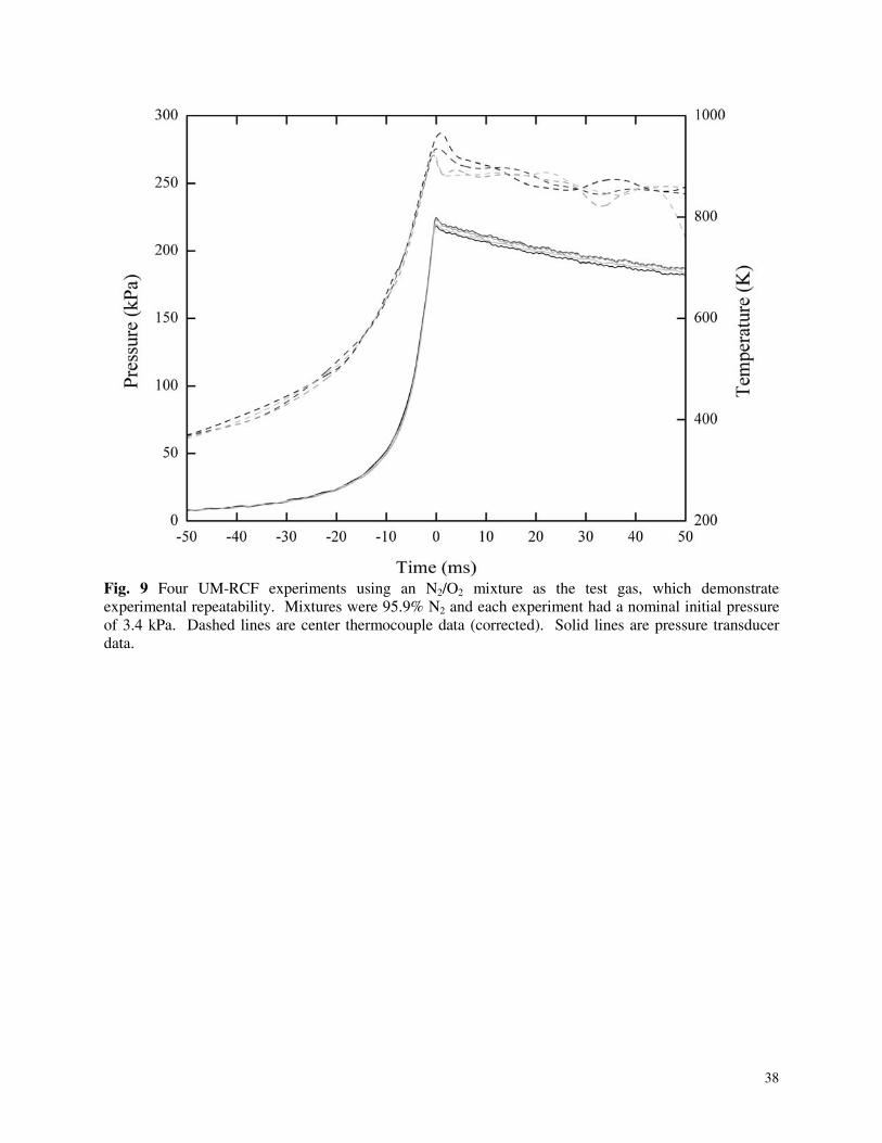
Figure 9 shows the results of four UM-RCF experiments (including data from Fig. 6)

using an N2/O2 mixture as the test gas, each with initial pressures of approximately 3.4 kPa (25.3

torr). Figure 10 shows a similar set of four UM-RCF experiments (including the data from

Fig. 8) conducted using Ar as the test gas. In each of these experiments, the initial Ar pressure is

approximately 6 kPa (45 torr).

Figures 9 and 10 demonstrate the UM-RCF is capable of generating very repeatable test

conditions. The variability in peak pressures is within 3% for both sets of data, and in both sets

of data the individual pressure histories follow nearly identical trajectories. The small

differences observed in the individual pressure histories can be readily attributed to run-to-run

uncertainties in initial pressures, drive pressures, frictional forces, and fluid behavior. As with

the pressure histories, the temperature histories follow nearly identical trajectories during the

compression process. The divergence in the temperature histories after this point is primarily

due to the limitation of the methodology used to correct for the time response of the

thermocouples. This is addressed in further detail below.

Data Post-Processing

As noted above, the experimental data are post-processed. The impact of the sabot into the test

manifold creates pressure disturbances that are filtered from the data. Spectral analysis of these

disturbances indicates the frequencies of the disturbances are consistent with the frequencies at

which pressure waves traverse the test volume. These disturbances are not believed to be

16

representative of the mean pressure in the test manifold and are thought to be due to vibrations

created in the test manifold due to the forceful impact of the sabot into the test manifold. The

average magnitude of these disturbances is less than 3% of the peak pressure, with the maximum

disturbance being less than 10%. The magnitude of the disturbances correlates strongly with the

force of the impact of the sabot into the test manifold.

The raw data from the 25 µm diameter thermocouples (~80 µm bead diameter) are post-

processed to remove high-frequency electrical noise. The temperature measurements are also

corrected to account for radiation heat transfer and the time response of the thermocouples. Due

to their thermal mass, the temperature measured by the thermocouples lags the actual gas

temperature. Failure to make this correction results in an under-prediction of peak temperatures

and temperature profiles which are temporally displaced from the actual gas temperatures. The

actual gas temperature (Tg) is related to the measured temperature Tm by the relation

( )44mmg wm TT

hdt

dTTT −++= εστ , where the time constant of the thermocouple is

τ = ρcd 2

4k ⋅ Nu(where ρ, c and d are the density, heat capacity and diameter of the thermocouple

wire, respectively, k is the thermal conductivity of the gas, and Nu is the Nusselt number), the

emissivity of the thermocouple is ε, the average heat transfer coefficient is h , and the

temperature of the RCF walls is Tw. The time responses of the thermocouples vary based on

experimental conditions, primarily due to differences in gas properties (density, thermal

conductivity, and viscosity) and gas velocity, which affects the Nusselt number. The

thermocouple time response is also a function of time, as the parameters on which it is based

vary during the course of the compression process.

17

For the data presented here, the thermocouple time constants are determined individually

for each experiment. The time constant is calculated based on instantaneous gas properties

(temperature, density, etc.) and standard correlations for convective heat transfer to a sphere.

Based on these calculations, the uncertainty in the corrected temperature during compression is

estimated to be ±5%. Uncertainties at times after the point of peak pressure are expected to be

greater because the thermocouple correction model does not accurately represent the actual fluid

dynamics within the test volume after the sabot nose cone has come to rest.

Experimental Modeling

Analytical models that can be used to predict RCF performance (peak temperature and pressure)

for a given set of operating conditions are valuable aids to the design of experiments using RCFs.

Because compression of the test gases is rapid (the entire compression process occurs in

approximately 100 ms, with the bulk of the compression occurring in the last 10 ms), as a first

approximation the compression process can be considered to occur isentropically. Modeling the

compression as an isentropic process provides an upper bound on the temperature and pressure

that can be generated by the UM-RCF for non-reacting test gas mixtures.

Using the isentropic relations for an ideal gas, the pressure and temperature depend only

on the compression ratio (CR) and the ratio of the specific heats of the compressed gas mixture

(γ = Cp/Cv), where CR is defined as the ratio of the initial molar specific volume ( v o) to the

molar specific volume at the end of compression ( v max). With Po and To as the initial pressure

and temperature, the peak pressure and temperature (Pmax and Tmax, respectively) can be

calculated using the following relations:

1γ

d ln P = lnv o

v maxPo

Pmax∫ = lnCR (1)

18

1

γ −1d lnT = ln

v ov max

= lnCRTo

Tmax∫ (2)

For a non-monatomic gas, Eqns (1) and (2) must be solved by direct integration. For the

case of a monatomic test gas, γ is a constant and Eqns (1) and (2) simplify to:

Pmax

Po

= CRγ (3)

Tmax

To

= CRγ −1 (4)

Adopting an appropriate average value for γ, Eqns (3) and (4) may be applied to non-

monatomic gases. While Eqns (3) and (4) are not used for the analysis of the UM-RCF data

presented in the current work (with the exception of experiments with argon as the test gas), they

do provide a convenient method for the evaluation of isentropic conditions for non-monatomic

gases and will be used here to simplify the discussion of the compression process.

Two issues arise in the use of Eqns (3) and (4) to model the compression process in the

UM-RCF: what is the appropriate compression ratio and is the compression process truly

isentropic? Defining the compression ratio is not straightforward with the UM-RCF. In a typical

control mass piston-cylinder arrangement, the compression ratio would be defined simply as the

ratio of the initial (pre-compression) volume to the final (post-compression) volume. With the

UM-RCF, the stepped nature of the “cylinder” and “piston” along with the possibility of mass

outflow from the test volume (past the U-ring seals and into the driver gases) complicate using

such a definition for the compression ratio.

To deal with the difficulty of defining a compression ratio in the traditional sense, an

effective compression ratio (CR') was defined based on the ratio of the post-test pressure to the

initial pressure. As will be shown below, this compression ratio is the same ratio as used in Eqns

(1) to (4); it is just calculated differently. Using the ideal gas equation of state (where P is the

19

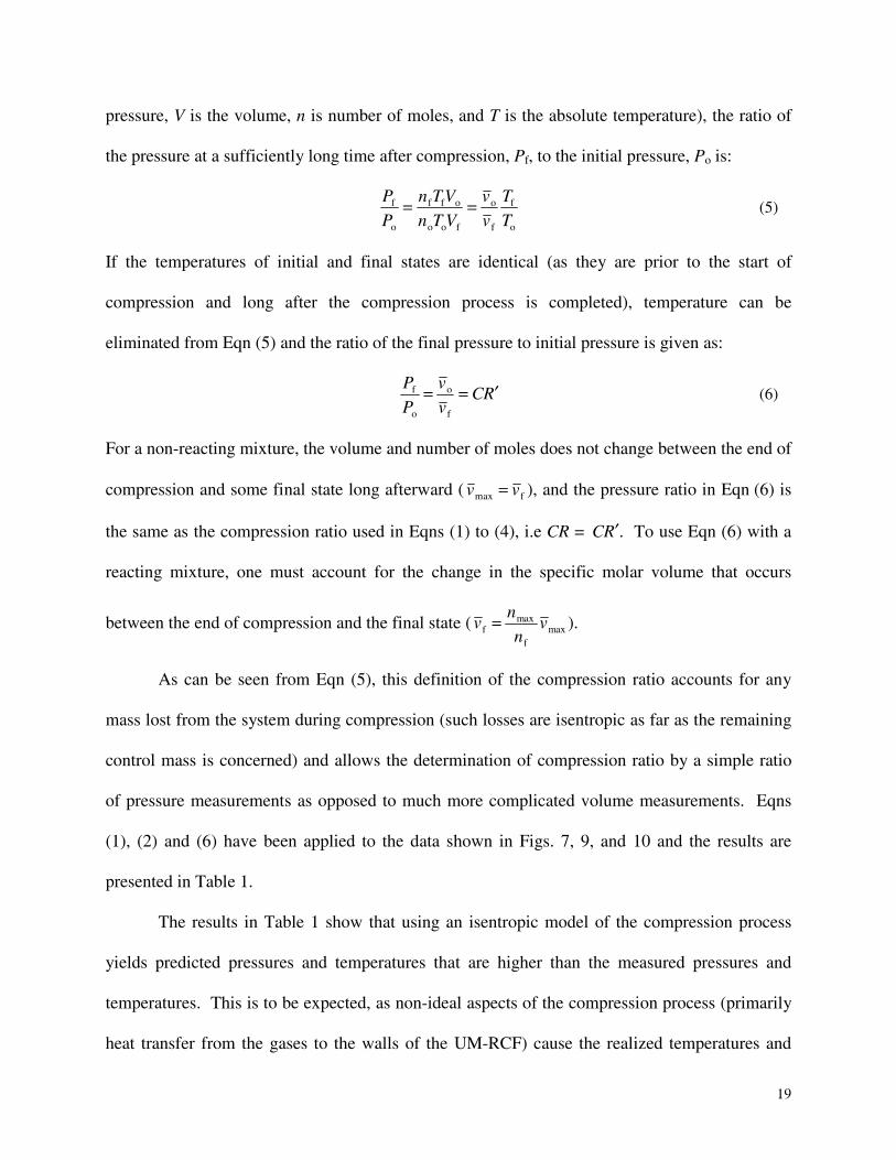
pressure, V is the volume, n is number of moles, and T is the absolute temperature), the ratio of

the pressure at a sufficiently long time after compression, Pf, to the initial pressure, Po is:

Pf

Po

= nfTfVo

noToVf

= v ov f

Tf

To

(5)

If the temperatures of initial and final states are identical (as they are prior to the start of

compression and long after the compression process is completed), temperature can be

eliminated from Eqn (5) and the ratio of the final pressure to initial pressure is given as:

Pf

Po

= v ov f

= C ′R (6)

For a non-reacting mixture, the volume and number of moles does not change between the end of

compression and some final state long afterward ( v max = v f ), and the pressure ratio in Eqn (6) is

the same as the compression ratio used in Eqns (1) to (4), i.e CR = C ′R . To use Eqn (6) with a

reacting mixture, one must account for the change in the specific molar volume that occurs

between the end of compression and the final state ( v f = nmax

nf

v max ).

As can be seen from Eqn (5), this definition of the compression ratio accounts for any

mass lost from the system during compression (such losses are isentropic as far as the remaining

control mass is concerned) and allows the determination of compression ratio by a simple ratio

of pressure measurements as opposed to much more complicated volume measurements. Eqns

(1), (2) and (6) have been applied to the data shown in Figs. 7, 9, and 10 and the results are

presented in Table 1.

The results in Table 1 show that using an isentropic model of the compression process

yields predicted pressures and temperatures that are higher than the measured pressures and

temperatures. This is to be expected, as non-ideal aspects of the compression process (primarily

heat transfer from the gases to the walls of the UM-RCF) cause the realized temperatures and

20

pressures to depart from those predicted by an isentropic analysis. Worth noting is how the

accuracy of the isentropic model depends on the test gas mixture and the test conditions. Since

heat transfer to the walls is proportional to kf/ρfCp,f (where kf, ρf and Cp,f are the thermal

conductivity, density, and the constant pressure heat capacity of the gas, respectively), it is

reasonable to expect a gas mixture with a higher density and heat capacity to be less affected by

cooling at the walls. As heat transfer to the walls is also proportional to the temperature

difference between the bulk gas and the walls, a cooler gas will lose heat at a lower rate to the

walls. These conclusions are supported by the results of Table 1 where the over-prediction of

pressure is 6% for N2 as the test gas (ρfCp,f = 8250 J/m3-K, ∆T ≈ 690 K), 13% for the N2/O2

mixtures (ρfCp,f = 1000, ∆T ≈ 645 K), and 24% for argon as the test gas (ρfCp,f = 1080 ∆T ≈ 1700

K). For these calculations, ρf is determined from the final temperature and pressure, Cp,f is

calculated at the peak temperature, and ∆T is the difference between the maximum gas

temperature and the wall temperature. (It should be noted that the difference in ρfCp,f between

the N2 and the N2/O2 mixtures is due largely to the differences in the density which are due to the

different initial pressures of these two mixtures: 26.7 and 3.37 kPa, respectively.) The thermal

conductivity, kf, is roughly identical for all the gas mixtures and is therefore omitted for clarity.

The N2 experiment has the highest ρfCp,f and nearly the lowest temperature differential.

Therefore, it is not surprising to find the N2 experimental results are best modeled with an

isentropic analysis. The N2/O2 and Ar data sets have nearly identical values of ρfCp,f, yet the

argon experiments have a temperature difference over 2.5 times that of the N2/O2 experiments.

This difference between the N2/O2 and Ar data is reflected in how well the data are represented

by the isentropic analysis. Despite the shortcomings of an isentropic model, this model can still

provide valuable insights into the compression process.

21

While the overall compression process is non-isentropic, is it realistic to assume that a

core region of the compressed gas is unaffected by heat transfer at the walls and is compressed in

an isentropic manner as suggested by other RCF researchers [29]. Having such a core region is

necessary to support the assumption that conditions within the (reacting) gas mixture can be

treated as (spatially) uniform. If non-isentropic effects, such as heat transfer and fluid motion,

were significant throughout the test gas volume, analysis and interpretation of RCF results would

be extremely difficult. As discussed previously, the rapid compression times (that minimize heat

transfer to the RCF walls) and the novel sabot design (that minimizes the effects of the boundary

layers on the bulk of the gas mixture) are features of the UM-RCF that are expected to promote

the existence of a core region which is compressed in an essentially isentropic manner.

Confirming the existence of this “isentropic core” then becomes a matter of a thermodynamic

calculation.

Based on the initial and maximum pressures (Po and Pmax), an effective compression ratio

(CReff) can be calculated for the core gas region by using the measured pressure time history, a

temperature-dependant expression for γ, and numerically integrating Eqn (1). Due to the effects

of heat transfer on the pressure of the test gases, CReff will naturally be lower than the physical

compression ratio determined using Eqn (6). Using this effective compression ratio, the

maximum gas temperature can be calculated and compared to the measured gas temperature as a

check on the accuracy of the measurement and the validity of the assumption of an isentropic gas

core region. For argon the process is much simpler as γ is independent of temperature and the

Tmax can be calculated directly by combining Eqns (3) and (4) to yield: Tmax = To(Pmax/Po)(γ-1)/γ.

These calculations have been applied to the data of Table 1 and the results are shown in Table 2.

22

As can be seen in Table 2, the predicted maximum temperatures are in very good

agreement with the measured temperatures (less than 5% difference for all conditions studied),

supporting the assumption of an “isentropic core.” Negative differences between the model

predictions and the measured temperatures are an indication of the limitations of the

thermocouple measurements. Additionally, this technique can be applied to mixtures that react

subsequent to the compression process. The comparison between measured and calculated

maximum temperatures can also be used to determine if reaction occurs during the compression

process.

Temperature Distribution in the UM-RCF

While the existence of an isentropic core has been demonstrated, the extent of this core region is

unclear. For the assumption of an isentropic core to be useful for experimental studies, the radial

and axial extent of this region must be quantified. Based on the previous calculations, it is

reasonable to assume the isentropic core region encompasses the volume in which the

temperature is approximately that measured by the center thermocouple. To determine the extent

of this core region, simultaneous radial and axial temperature measurements were obtained at

several locations in the test manifold.

Radial temperature profiles were obtained using a thermocouple manifold equipped with

four thermocouples. The nominal locations of the thermocouple junctions were the center

(25.4 mm from the wall), 0.9 mm from the wall, and two intermediate locations. Two pairs of

intermediate locations were investigated: 2.9 and 10.4 mm from the wall and 5 and 7 mm from

the wall. Figures 11 and 12 present the temperature measurements from these two experiments

(all using nitrogen as the test gas) conducted using this thermocouple manifold. The measured

thermocouple temperatures were corrected as previously described. Data from the thermocouple

23

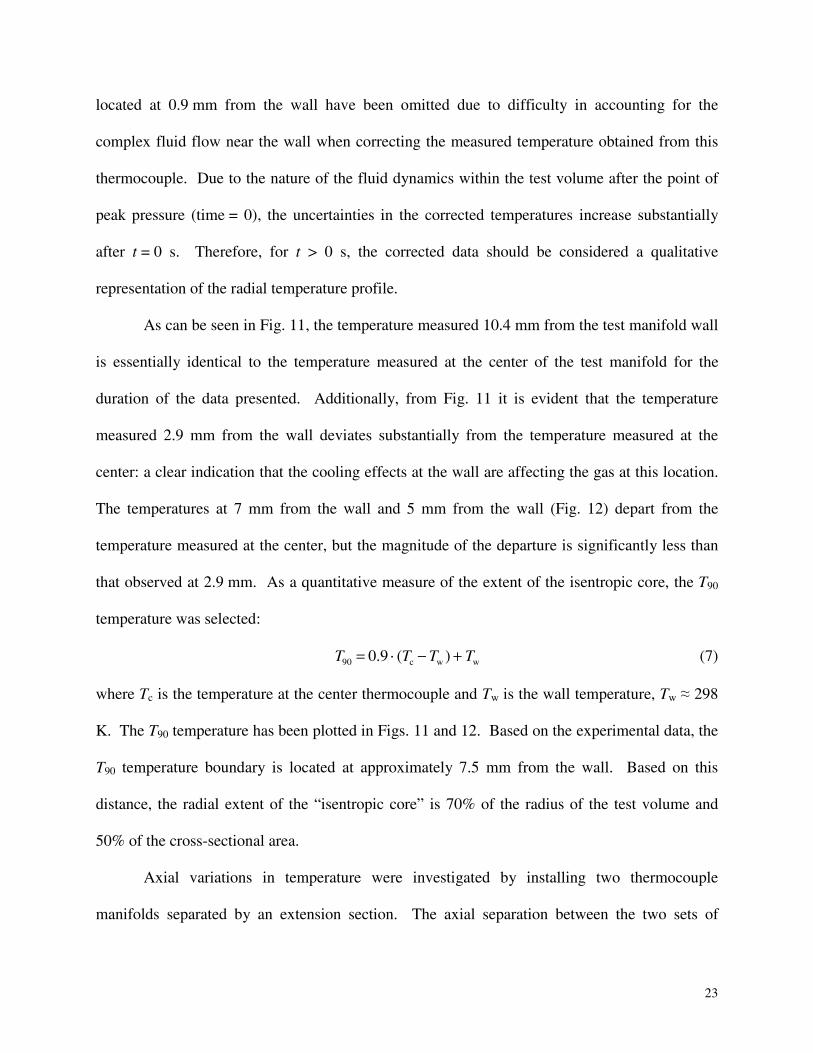
located at 0.9 mm from the wall have been omitted due to difficulty in accounting for the

complex fluid flow near the wall when correcting the measured temperature obtained from this

thermocouple. Due to the nature of the fluid dynamics within the test volume after the point of

peak pressure (time = 0), the uncertainties in the corrected temperatures increase substantially

after t = 0 s. Therefore, for t > 0 s, the corrected data should be considered a qualitative

representation of the radial temperature profile.

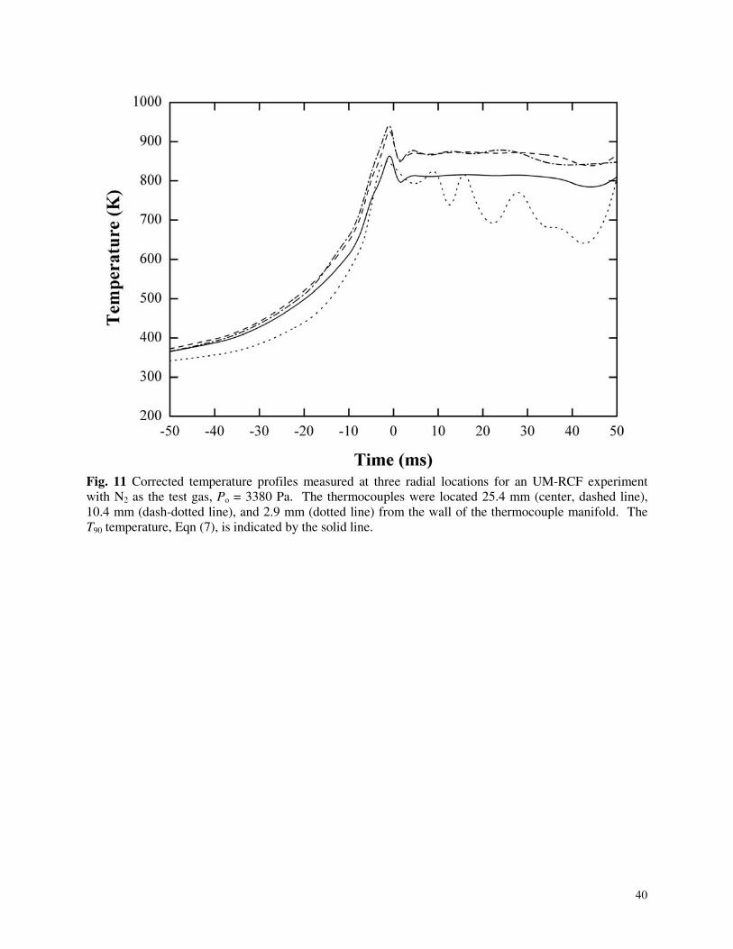
As can be seen in Fig. 11, the temperature measured 10.4 mm from the test manifold wall

is essentially identical to the temperature measured at the center of the test manifold for the

duration of the data presented. Additionally, from Fig. 11 it is evident that the temperature

measured 2.9 mm from the wall deviates substantially from the temperature measured at the

center: a clear indication that the cooling effects at the wall are affecting the gas at this location.

The temperatures at 7 mm from the wall and 5 mm from the wall (Fig. 12) depart from the

temperature measured at the center, but the magnitude of the departure is significantly less than

that observed at 2.9 mm. As a quantitative measure of the extent of the isentropic core, the T90

temperature was selected:

T90 = 0.9 ⋅ (Tc − Tw ) + Tw (7)

where Tc is the temperature at the center thermocouple and Tw is the wall temperature, Tw ≈ 298

K. The T90 temperature has been plotted in Figs. 11 and 12. Based on the experimental data, the

T90 temperature boundary is located at approximately 7.5 mm from the wall. Based on this

distance, the radial extent of the “isentropic core” is 70% of the radius of the test volume and

50% of the cross-sectional area.

Axial variations in temperature were investigated by installing two thermocouple

manifolds separated by an extension section. The axial separation between the two sets of

24

thermocouples was 106 mm. The experiments were conducted with nitrogen as the test gas at

conditions similar to those in Fig. 6. Figure 13 presents a typical data set from these

investigations. As can be seen from the figure, there are negligible differences between the

temperatures at the two axial locations. The small differences seen post-compression (t > 0 s)

are more due to uncertainties with the temperature correction technique (discussed previously)

than differences in the thermocouple measurements. Based on these data, axial variations in

temperature within the test volume (away from the end wall and the sabot) are considered

negligible within the time frame of the experiments.

Reactive Mixture Experiment

As a further demonstration of the capabilities of the UM-RCF, the results of an early

investigation into iso-octane ignition are presented in Fig. 14. The test gas mixture for this

experiment was 0.53% C8H18, 16.59% O2, 10.01% Ar, and balance N2 (equivalence ratio ≈ 0.4).

The initial pressure was 18.1 kPa (136 torr) and the nominal calculated compression ratio (CR´)

was 26.1. In addition to the pressure data, Fig. 14 includes emission recorded by an un-amplified

silicon photodiode detector (Hamamatsu S1787-3).

The measured pressure at the end of the compression process is 1630 kPa. Using this

pressure and the initial pressure of 18.1 kPa in Eqn. (6), the isentropic core temperature (prior to

reaction) is calculated to be 991 K. As can also be seen in Fig. 14, the start of the emission

signal corresponds extremely well with the increase in pressure due to ignition. The calculated

ignition delay time is approximately 8 ms. The iso-octane ignition data serve to demonstrate the

potential of the UM-RCF for studies of reacting mixtures using the conditions and performance

validated by the non-reacting studies.

25

4. Conclusions

The current work demonstrates the suitability of the UM-RCF as an experimental tool for

the study of combustion phenomena. As can be seen in Table 3, the experimental conditions that

can be achieved with the UM-RCF expand the envelope of RCF operating conditions, which

increases the usefulness of the RCF as a research tool. The diagnostics available with the UM-

RCF (pressure, temperature, optical diagnostics, and high speed video capture) also expand the

range of data that can be obtained from RCF experiments.

The characterization data show that the UM-RCF can rapidly generate and sustain the

high temperatures and pressures found in many combustion systems of interest. The high

temperature (greater than 80% Tmax) and high pressure (greater than 75% Pmax) test conditions

can be maintained for durations substantially longer than those obtainable with shock tubes or

demonstrated by other rapid-compression facilities (i.e. 50 ms and greater, depending on the test

gas densities and heat capacities). The data show excellent test repeatability, with a run-to-run

variability of less than 3% (based on pressure measurements). Analysis of the data indicates the

existence of a core region of the test gas which is compressed isentropically and has nominally

uniform conditions. This core region extends across 70% of the diameter of the test section and

contains approximately 50% of the test gas volume. Existence of such a region is essential to

maximizing the utility of the UM-RCF as a combustion research tool. These beneficial aspects

of the state conditions found in the UM-RCF experiments are direct results of the unique design

of the UM facility. The high pressures, moderate temperatures, and long test times make the

UM-RCF an ideal facility to complement other chemical reactor studies.

26

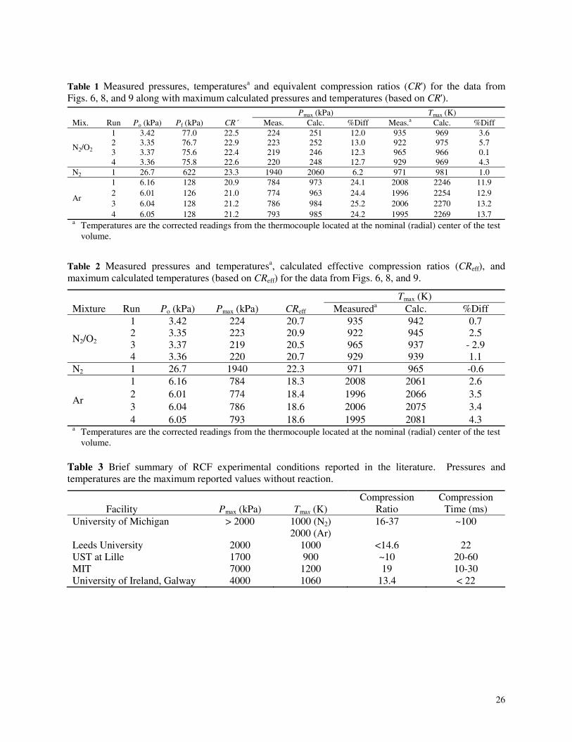
Table 1 Measured pressures, temperaturesa and equivalent compression ratios (CR') for the data from Figs. 6, 8, and 9 along with maximum calculated pressures and temperatures (based on CR').

Pmax (kPa) Tmax (K) Mix. Run Po (kPa) Pf (kPa) CR´ Meas. Calc. %Diff Meas.a Calc. %Diff

1 3.42 77.0 22.5 224 251 12.0 935 969 3.6 2 3.35 76.7 22.9 223 252 13.0 922 975 5.7 3 3.37 75.6 22.4 219 246 12.3 965 966 0.1

N2/O2

4 3.36 75.8 22.6 220 248 12.7 929 969 4.3 N2 1 26.7 622 23.3 1940 2060 6.2 971 981 1.0

1 6.16 128 20.9 784 973 24.1 2008 2246 11.9 2 6.01 126 21.0 774 963 24.4 1996 2254 12.9 3 6.04 128 21.2 786 984 25.2 2006 2270 13.2

Ar

4 6.05 128 21.2 793 985 24.2 1995 2269 13.7 a Temperatures are the corrected readings from the thermocouple located at the nominal (radial) center of the test

volume.

Table 2 Measured pressures and temperaturesa, calculated effective compression ratios (CReff), and maximum calculated temperatures (based on CReff) for the data from Figs. 6, 8, and 9.

Tmax (K) Mixture Run Po (kPa) Pmax (kPa) CReff Measureda Calc. %Diff

1 3.42 224 20.7 935 942 0.7 2 3.35 223 20.9 922 945 2.5 3 3.37 219 20.5 965 937 - 2.9

N2/O2

4 3.36 220 20.7 929 939 1.1 N2 1 26.7 1940 22.3 971 965 -0.6

1 6.16 784 18.3 2008 2061 2.6 2 6.01 774 18.4 1996 2066 3.5 3 6.04 786 18.6 2006 2075 3.4

Ar

4 6.05 793 18.6 1995 2081 4.3 a Temperatures are the corrected readings from the thermocouple located at the nominal (radial) center of the test

volume. Table 3 Brief summary of RCF experimental conditions reported in the literature. Pressures and temperatures are the maximum reported values without reaction.

Facility Pmax (kPa) Tmax (K) Compression

Ratio Compression

Time (ms) University of Michigan > 2000 1000 (N2)

2000 (Ar) 16-37 ~100

Leeds University 2000 1000 <14.6 22 UST at Lille 1700 900 ~10 20-60 MIT 7000 1200 19 10-30 University of Ireland, Galway 4000 1060 13.4 < 22

27

Fig. 1 Schematic and photograph of the University of Michigan Rapid Compression Facility.

Fig. 2 End view of the thermocouple manifold showing typical placement of two fine wire

thermocouples.

Fig. 3 Cross-sectional view of the UM-RCF test section. Optical and instrument ports are shown with

the ports removed.

Fig. 4 Photograph of the UM-RCF sabot. The black portion is the Delrin™ body and the white portion

is the UHMW replaceable nose cone. The two U-ring seals can be seen on Delrin™ section of the sabot.

Fig. 5 Depiction of the UM-RCF in operation. a) Driven section is charged with the test gas mixture

prior to start of test. Driver section is charged with high-pressure air. b) Hydraulic valve is opened and

high-pressure gas from the driver section propels the sabot down the length of the driven section. c)

Sabot travels down the length of the driven section, compressing the test gas mixture ahead of the sabot.

d) Sabot is lodged in the extension section, trapping the test gas mixture within the test manifold. The

annular region of the test gas mixture, which includes most of the fluid disturbances caused by the travel

of the sabot down the length of the driven section, is trapped in the shoulder region.

Fig. 6 Typical pressure and temperature time-histories from an UM-RCF experiment using an N2/O2

mixture as the test gas (95.9% N2, balance O2), Po = 3.37 kPa. The inset shows raw pressure and

temperature traces.

Fig. 7 Typical pressure and temperature time-histories from an UM-RCF experiment using N2 as the test

gas, Po = 26.7 kPa.

Fig. 8 Typical pressure and temperature time-histories from an UM-RCF experiment using Ar as the test

gas, Po = 6.01 kPa.

Fig. 9 Four UM-RCF experiments using an N2/O2 mixture as the test gas, which demonstrate

experimental repeatability. Mixtures were 95.9% N2 and each experiment had a nominal initial pressure

28

of 3.4 kPa. Dashed lines are center thermocouple data (corrected). Solid lines are pressure transducer

data.

Fig. 10 Four UM-RCF experiments using Ar as the test gas, which demonstrate experimental

repeatability. Each experiment had a nominal initial pressure of 6.0 kPa. Dashed lines are center

thermocouple data (corrected). Solid lines are pressure transducer data.

Fig. 11 Corrected temperature profiles measured at three radial locations for an UM-RCF experiment

with N2 as the test gas, Po = 3380 Pa. The thermocouples were located 25.4 mm (center, dashed line),

10.4 mm (dash-dotted line), and 2.9 mm (dotted line) from the wall of the thermocouple manifold. The

T90 temperature, Eqn (7), is indicated by the solid line.

Fig. 12 Corrected temperature profiles measured at three radial locations for an UM-RCF experiment

with N2 as the test gas, Po = 4560 Pa. The thermocouples were located 25.4 mm (dashed line), 7 mm

(dash-dotted line), and 5 mm (dotted line) from the wall of the thermocouple manifold. The T90

temperature, Eqn (7), is indicated by the solid line.

Fig. 13 Corrected temperature profiles at two axial locations for an UM-RCF experiment with N2 as the

test gas, Po = 4560 Pa. The thermocouples were located at the radial center of the test manifold and at

64 mm (dashed line) and 170 (solid line) mm from the end wall.

Fig. 14 Typical pressure (solid line) and light-emission (dashed line) time-histories from an UM-RCF

experiment using C8H18/O2/Ar/N2 (mole fractions of 0.0053, 0.1659, 0.1001, respectively, balance N2) as

the test gas, Po = 18.1 kPa.

29

5540mm 2740mm

ID=154mm ID=101.2mm

Driver Section

Hydraulic Valve

Driven Section

Convergent Section

Temperature Measurement Section

Test Section

Photo DetectorExtension Section

Diode Laser

Test Manifold

Fig. 1 Schematic and photograph of the University of Michigan Rapid Compression Facility.

30

Fig. 2 End view of the thermocouple manifold showing typical placement of two fine wire thermocouples.

31

Fig. 3 Cross-sectional view of the UM-RCF test section. Optical and instrument ports are shown with the ports removed.

32

Fig. 4 Photograph of the UM-RCF sabot. The black portion is the Delrin™ body and the white portion is the UHMW replaceable nose cone. The two U-ring seals can be seen on Delrin™ section of the sabot.

33

Fig. 5 Depiction of the UM-RCF in operation. a) Driven section is charged with the test gas mixture prior to start of test. Driver section is charged with high-pressure air. b) Hydraulic valve is opened and high-pressure gas from the driver section propels the sabot down the length of the driven section. c) Sabot travels down the length of the driven section, compressing the test gas mixture ahead of the sabot. d)

34

Sabot is lodged in the extension section, trapping the test gas mixture within the test manifold. The annular region of the test gas mixture, which includes most of the fluid disturbances caused by the travel of the sabot down the length of the driven section, is trapped in the shoulder region.

35

Fig. 6 Typical pressure and temperature time-histories from an UM-RCF experiment using an N2/O2 mixture as the test gas (95.9% N2, balance O2), Po = 3.37 kPa. The inset shows raw pressure and temperature traces.

36

Fig. 7 Typical pressure and temperature time-histories from an UM-RCF experiment using N2 as the test gas, Po = 26.7 kPa.

37

Fig. 8 Typical pressure and temperature time-histories from an UM-RCF experiment using Ar as the test gas, Po = 6.01 kPa.

38

Fig. 9 Four UM-RCF experiments using an N2/O2 mixture as the test gas, which demonstrate experimental repeatability. Mixtures were 95.9% N2 and each experiment had a nominal initial pressure of 3.4 kPa. Dashed lines are center thermocouple data (corrected). Solid lines are pressure transducer data.

39

Fig. 10 Four UM-RCF experiments using Ar as the test gas, which demonstrate experimental repeatability. Each experiment had a nominal initial pressure of 6.0 kPa. Dashed lines are center thermocouple data (corrected). Solid lines are pressure transducer data.

40

Fig. 11 Corrected temperature profiles measured at three radial locations for an UM-RCF experiment with N2 as the test gas, Po = 3380 Pa. The thermocouples were located 25.4 mm (center, dashed line), 10.4 mm (dash-dotted line), and 2.9 mm (dotted line) from the wall of the thermocouple manifold. The T90 temperature, Eqn (7), is indicated by the solid line.

41

Fig. 12 Corrected temperature profiles measured at three radial locations for an UM-RCF experiment with N2 as the test gas, Po = 4560 Pa. The thermocouples were located 25.4 mm (dashed line), 7 mm (dash-dotted line), and 5 mm (dotted line) from the wall of the thermocouple manifold. The T90 temperature, Eqn (7), is indicated by the solid line.

42

Fig. 13 Corrected temperature profiles at two axial locations for an UM-RCF experiment with N2 as the test gas, Po = 4560 Pa. The thermocouples were located at the radial center of the test manifold and at 64 mm (dashed line) and 170 (solid line) mm from the end wall.

43

Fig. 14 Typical pressure (solid line) and light-emission (dashed line) time-histories from an UM-RCF experiment using C8H18/O2/Ar/N2 (mole fractions of 0.0053, 0.1659, 0.1001, respectively, balance N2) as the test gas, Po = 18.1 kPa.

44

References 1. H. Kellerer, A. Müller, H.-J. Bauer, and S. Wittig, Combust. Sci. Tech. 113-114 (1996) 67-

80.

2. C. K. Westbrook, W. J. Pitz, J. E. Boercker, H. J. Curran, J. F. Griffiths, C. Mohamed, and

M. Ribaucour, Proc. Combust. Inst. 29 (2002) 1331-1318.

3. K. Epping, S. Aceves, and J. Dec, Society of Automotive Engineers SAE-2002-01-1923

(2002).

4. S.-M. Suh, M. R. Zachariah, and S. L. Girshick, J. Vac. Sci. Technol. A 19(3) (2001) 940-

951.

5. A. G. Gaydon and I. R. Hurle, The Shock Tube in High-Temperature Chemical Physics.

Reinhold Publishing, New York, NY, 1963.

6. P. Beeley, J. F. Griffiths, and P. Gray, Combust. Flame 39 (1980) 255-268.

7. J. F. Griffiths, P. A. Halford-Maw, and D. J. Rose, Combust. Flame 95 (1993) 291-306.

8. A. Cox, J. F. Griffiths, C. Mohamed, H. J. Curran, W. J. Pitz, and C. K. Westbrook, Proc.

Comb. Inst. 26 (1996) 2685-2692.

9. J. Clarkson, J. F. Griffiths, J. P. MacNamara, and B. J. Whitaker, Combust. Flame 125

(2001) 1162-1175.

10. J. F. Griffiths, Q. Jiao, M. Schreiber, J. Meyer, and K. F. Knoche, Proc. Comb. Inst. 24

(1992) 1809-1815.

11. C. K. Westbrook, H. J. Curran, W. J. Pitz, J. F. Griffiths, C. Mohamed, and S. K. Wo, Proc.

Comb. Inst. 27 (1998) 371-378.

12. J. F. Griffiths and B. J. Whitaker, Combust. Flame 131 (2002) 386-399.

13. M. Ribaucour, R. Minetti, and L . R. Sochet, Proc. Comb. Inst. 27 (1998) 345-351.

45

14. R. Minetti, M. Carlier, M. Ribaucour, E. Therssen, and L. R. Sochet, Combust. Flame 102

(1995) 298-309.

15. R. Minetti, M. Carlier, M. Ribaucour, E. Therssen, and L. R. Sochet, Proc. Comb. Inst. 26

(1996) 747-753.

16. R. Minetti, M. Ribaucour, M. Carlier, and L. R. Sochet, Combust. Sci. Tech. 113-114 (1996)

179-192.

17. P. Desgroux, L. Gasnot, and L. R. Sochet, Appl. Phys. B 61 (1995) 69-72.

18. P. Desgroux, R. Minetti, and L. R. Sochet, Combust. Sci. Technol. 113-114 (1996) 193-203.

19. M. Ribaucour, R. Minetti, L. R. Sochet, H. J. Curran, W. J. Pitz, and C. K. Westbrook, Proc.

Comb. Inst. 28 (2000) 1671-1678.

20. P. Park, and J. C. Keck, Society of Automotive Engineers SAE-900027 (1990).

21. D. Lee and S. Hochgreb, Int. J. Chem. Kinet. 30 (1998) 385-406.

22. D. Lee and S. Hochgreb, Combust. Flame 114 (1998) 531-545.

23. S. Tanaka, F. Ayala, J. C. Keck, and J. B. Heywood, Combust. Flame 132 (2003) 219-239.

24. S. Tanaka, F. Ayala, and J. C. Keck, Combust. Flame 133 (2003) 467-481.

25. L. Brett, J. MacNamara, P. Musch, and J. M. Simmie, Combust. Flame 124 (2001) 326-329.

26. S. M. Gallagher, H. J. Curran, J. Würmel, J., and J. M. Simmie, “The Oxidation of Propane at

Elevated Pressures in a Rapid-Compression Machine. An Experimental and Modeling

Study,” Proceedings of the Third Joint Meeting of the U.S. Sections of The Combustion

Institute, Chicago, IL, USA, March 2003.

27. W. S. Affleck and A. Thomas, Proc. Inst. Mech. Eng. 183 (1969) 365-385.

28. G. F. Carrier, F. E. Fendell, C. T. Hsu, I. L. Stonich, and L. D. Bergerson, Basic Research on

Flame Radiation, Report 91/0091, Gas Research Institute, 1991.

46

29. J. F. Griffiths, Q. Jiao, W. Kordylewski, M. Schreiber, J. Meyer, and K. F. Knoche, Combust.

Flame 93 (1993) 303-315.