Demonstrating Lambda Calculus Reduction

Peter Sestoft

Department of Mathematics and PhysicsRoyal Veterinary and Agricultural University, Denmark

and

IT University of Copenhagen, Denmark

sestoft@dina.kvl.dk

Abstract. We describe lambda calculus reduction strategies, such ascall-by-value, call-by-name, normal order, and applicative order, usingbig-step operational semantics. We show how to simply and efficientlytrace such reductions, and use this in a web-based lambda calculus re-ducer available at 〈http://www.dina.kvl.dk/˜sestoft/lamreduce/〉.

1 Introduction

The pure untyped lambda calculus is often taught as part of the computer sci-ence curriculum. It may be taught in a computability course as a classical com-putation model. It may be taught in a semantics course as the foundation fordenotational semantics. It may be taught in a functional programming courseas the archetypical minimal functional programming language. It may be taughtin a programming language course for the same reason, or to demonstrate thata very small language can be universal, e.g. can encode arithmetics (as well asdata structures, recursive function definitions and so on), using encodings suchas these:

two ≡ λf.λx.f(fx)four ≡ λf.λx.f(f(f(fx)))

add ≡ λm.λn.λf.λx.mf(nfx)(1)

This paper is motivated by the assumption that to appreciate the operationalaspects of pure untyped lambda calculus, students must experiment with it, andthat tools encourage experimentation with encodings and reduction strategiesby making it less tedious and more fun.

In this paper we describe a simple way to create a tool for demonstratinglambda calculus reduction. Instead of describing a reduction strategy by a pro-cedure for locating the next redex to be contracted, we describe it by a big-stepoperational semantics. We show how to trace the β-reductions performed duringreduction.

To do this we also precisely define and clarify the relation between program-ming language concepts such as call-by-name and call-by-value, and lambda cal-culus concepts such as normal order reduction and applicative order reduction.These have been given a number of different interpretations in the literature.

In T. Mogensen, D. Schmidt, I. H. Sudburough (editors): The Essence of Computation:

Complexity, Analysis, Transformation. Essays Dedicated to Neil D. Jones. Lecture

Notes in Computer Science 2566, pages 420-435. Springer-Verlag 2002.

2 Motivation and Related Work

Much has been written about the lambda calculus since Church developed itas a foundation for mathematics [6]. Landin defined the semantics of program-ming languages in terms of the lambda calculus [11], and gave a call-by-valueinterpreter for it: the secd-machine [10]. Strachey used lambda calculus as ameta-language for denotational semantics, and Scott gave models for the pureuntyped lambda calculus, making sure that self-application could be assigned ameaning; see Stoy [22]. Self-application (x x) of a term x is used when encodingrecursion, for instance in Church’s Y combinator:

Y ≡ λh.(λx.h (x x)) (λx.h (x x)) (2)

Plotkin studied the call-by-value lambda calculus corresponding to the func-tional language iswim [12] implemented by Landin’s secd-machine, and also arelated call-by-name lambda calculus, and observed that one characteristic of afunctional programming language was the absence of reduction under lambdaabstractions [19].

Barendregt [4] is the standard reference on the untyped lambda calculus,with emphasis on models and proof theory, not programming languages.

Many textbooks on functional programming or denotational semantics presentthe pure untyped lambda calculus, show how to encode numbers and algebraicdata types, and define evaluators for it. One example is Paulson’s ML textbook[16], which gives interpreters for call-by-name as well as call-by-value.

So is there really a need for yet another paper on lambda calculus reduction?We do think so, because it is customary to look at the lambda calculus eitherfrom the programming language side or from the calculus or model side, leavingthe relations between the sides somewhat unclear.

For example, Plotkin [19] defines call-by-value reduction as well as call-by-name reduction, but the call-by-name rules take free variables into account onlyto a limited extent. By the rules, x ((λz.z) v) reduces to x v, but (x y) ((λz.z) v)does not reduce to x y v [19, page 146]. Similarly, the call-by-value strategy de-scribed by Felleisen and Hieb using evaluation contexts [8, Section 2] would notreduce (x y) ((λz.z) v) to x y v, since there is no evaluation context of the form(x y) [ ]. This is unproblematic because, following Landin, these researchers wereinterested only in terms with no free variables, and in reduction only outsidelambda abstractions.

But it means that the reduction rules are not immediately useful for termsthat have free variables, and therefore not useful for experimentation with theterms that result from encoding programming language constructs in the purelambda calculus.

Conversely, Paulson [16] presents call-by-value and call-by-name interpretersfor the pure lambda calculus that do handle free variables. However, they alsoperform reduction under lambda abstractions (unlike functional programminglanguages), and the evaluation order is not leftmost outermost: under call-by-name, an application (e1 e2) is reduced by first reducing e1 to head normal form,

421

so redexes inside e1 may be contracted before an enclosing leftmost redex. Thismakes the relation between Paulson’s call-by-name and normal order (leftmostoutermost) reduction strategies somewhat unclear.

Therefore we find that it may be useful to contrast the various reductionstrategies, present them using big-step operational semantics, present their (naive)implementation in ML, and show how to obtain a trace of the reduction.

3 The Pure Untyped Lambda Calculus

We use the pure untyped lambda calculus [4]. A lambda term is a variable x,a lambda abstraction λx.e which binds x in e, or an application (e1 e2) of a‘function’ e1 to an ‘argument’ e2:

e ::= x | λx.e | e1 e2 (3)

Application associates to the left, so (e1 e2 e3) means ((e1 e2) e3). A lambda termmay have free variables, not bound by any enclosing lambda abstraction. Termidentity e1 ≡ e2 is taken modulo renaming of lambda-bound variables. Thenotation e[ex/x] denotes substitution of ex for x in e, with renaming of boundvariables in e if necessary to avoid capture of free variables in ex.

A redex is a subterm of the form ((λx.e) e2); the contraction of a redex pro-duces e[e2/x], substituting the argument e2 for every occurrence of the parameterx in e. By e −→β e′ we denote β-reduction, the contraction of some redex in eto obtain e′.

A redex is to the left of another redex if its lambda abstractor appearsfurther to the left. The leftmost outermost redex (if any) is the leftmost redexnot contained in any other redex. The leftmost innermost redex (if any) is theleftmost redex not containing any other redex.

4 Functional Programming Languages

In practical functional programming languages such as Scheme [20], StandardML [14] or Haskell [18], programs cannot have free variables, and reductions arenot performed under lambda abstractions or other variable binders, because thiswould considerably complicate their efficient implementation [17].

However, an implementation of lambda calculus reduction must perform re-ductions under lambda abstractions. Otherwise, add two two would not reduceto four using the encodings (1), which would disappoint students.

Because free variables and reduction under abstraction are absent in func-tional languages, it is unclear what the programming language concepts call-by-value and call-by-name mean in the lambda calculus. In particular, how shouldfree variables be handled, and to what normal form should call-by-value andcall-by-name evaluate? We propose the following answers:

422

– A free variable is similar to a data constructor (in Standard ML or Haskell),that is, an uninterpreted function symbol. If the free variable x is in functionposition (x e2), then call-by-value should reduce the argument expression e2,whereas call-by-name should not. This is consistent with constructors beingstrict in strict languages (e.g. ML) and non-strict in non-strict languages(e.g. Haskell).

– Functional languages perform no reduction under abstractions, and thusreduce terms to weak normal forms only. In particular, call-by-value reducesto weak normal form, and call-by-name reduces to weak head normal form.Section 6 define these normal forms.

5 Lazy Functional Programming Languages

Under lazy evaluation, a variable-bound term is evaluated at most once, regard-less how often the variable is used [17]. Thus an argument term may not beduplicated before it has been reduced, and may be reduced only if actually used.This evaluation mechanism may be called call-by-need, or call-by-name withsharing of argument evaluation. The equational theory of call-by-need lambdacalculus has been studied by Ariola and Felleisen [2] among others. (By con-trast, the lazy lambda calculus of Abramsky and Ong [1] is not lazy in the sensediscussed here; rather, it is the theory of call-by-name lambda calculus, withoutreduction under abstractions.)

Lazy functional languages also permit the creation of cyclic terms, or cyclesin the heap. For instance, this declaration creates a finite (cyclic) representationof an infinite list of 1’s:

val ones = 1 :: ones

Thus to be true also to the intensional properties of lazy languages (such as timeand space consumption), a model should be able to describe such constant-sizecyclic structures. Substitution of terms for variables cannot truly model them,only approximate them by unfolding of a recursive term definition, possiblyencoded using a recursion combinator such as (2). To properly express sharingof subterm evaluation, and the creation of cyclic terms, one must extend thesyntax (3) with mutually recursive bindings:

e ::= x | λx.e | e e | letrec xi = ei in e (4)

The sharing of subterm evaluation and the dynamic creation of cyclic terms maybe modelled using graph reduction, as suggested by Wadsworth [24] and used insubsequent work [3, 17, 23], or using an explicit heap [13, 21].

Thus a proper modelling of lazy evaluation, with sharing of argument evalu-ation and cyclic data structures, requires syntactic extensions as well as a moreelaborate evaluation model than just term rewriting. We shall not consider lazyevaluation any further in this paper, and shall consider only the syntax in (3)above.

423

6 Normal Forms

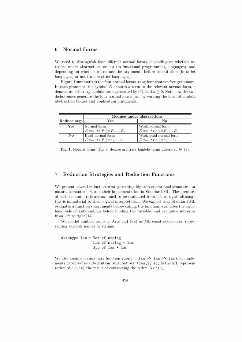
We need to distinguish four different normal forms, depending on whether wereduce under abstractions or not (in functional programming languages), anddepending on whether we reduce the arguments before substitution (in strictlanguages) or not (in non-strict languages).

Figure 1 summarizes the four normal forms using four context-free grammars.In each grammar, the symbol E denotes a term in the relevant normal form, edenotes an arbitrary lambda term generated by (3), and n ≥ 0. Note how the twodichotomies generate the four normal forms just by varying the form of lambdaabstraction bodies and application arguments.

Reduce under abstractions

Reduce args Yes No

Yes Normal formE ::= λx.E | xE1 . . . En

Weak normal formE ::= λx.e | x E1 . . . En

No Head normal formE ::= λx.E | x e1 . . . en

Weak head normal formE ::= λx.e | x e1 . . . en

Fig. 1. Normal forms. The ei denote arbitrary lambda terms generated by (3).

7 Reduction Strategies and Reduction Functions

We present several reduction strategies using big-step operational semantics, ornatural semantics [9], and their implementation in Standard ML. The premisesof each semantic rule are assumed to be evaluated from left to right, althoughthis is immaterial to their logical interpretation. We exploit that Standard MLevaluates a function’s arguments before calling the function, evaluates the right-hand side of let-bindings before binding the variable, and evaluates subtermsfrom left to right [14].

We model lambda terms x, λx.e and (e e) as ML constructed data, repre-senting variable names by strings:

datatype lam = Var of string

| Lam of string * lam

| App of lam * lam

We also assume an auxiliary function subst : lam -> lam -> lam that imple-ments capture-free substitution, so subst ex (Lam(x, e)) is the ML represen-tation of e[ex/x], the result of contracting the redex (λx.e) ex.

424

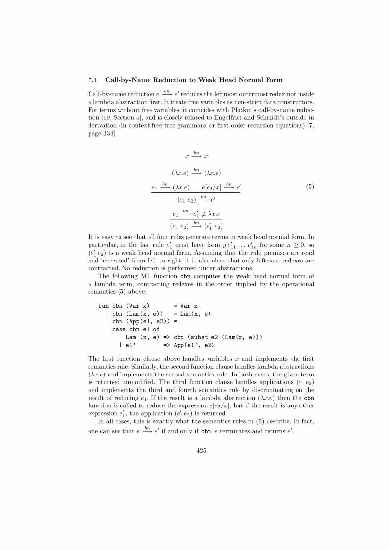
7.1 Call-by-Name Reduction to Weak Head Normal Form

Call-by-name reduction ebn−→ e′ reduces the leftmost outermost redex not inside

a lambda abstraction first. It treats free variables as non-strict data constructors.For terms without free variables, it coincides with Plotkin’s call-by-name reduc-tion [19, Section 5], and is closely related to Engelfriet and Schmidt’s outside-inderivation (in context-free tree grammars, or first-order recursion equations) [7,page 334].

xbn−→ x

(λx.e)bn−→ (λx.e)

e1bn−→ (λx.e) e[e2/x]

bn−→ e′

-----------------------------------------------------------------------------------------------------------------------------------------(e1 e2)

bn−→ e′

e1bn−→ e′1 6≡ λx.e

---------------------------------------------------------------------------------(e1 e2)

bn−→ (e′1 e2)

(5)

It is easy to see that all four rules generate terms in weak head normal form. Inparticular, in the last rule e′1 must have form y e′11 . . . e′1n for some n ≥ 0, so(e′1 e2) is a weak head normal form. Assuming that the rule premises are readand ‘executed’ from left to right, it is also clear that only leftmost redexes arecontracted. No reduction is performed under abstractions.

The following ML function cbn computes the weak head normal form ofa lambda term, contracting redexes in the order implied by the operationalsemantics (5) above:

fun cbn (Var x) = Var x

| cbn (Lam(x, e)) = Lam(x, e)

| cbn (App(e1, e2)) =

case cbn e1 of

Lam (x, e) => cbn (subst e2 (Lam(x, e)))

| e1’ => App(e1’, e2)

The first function clause above handles variables x and implements the firstsemantics rule. Similarly, the second function clause handles lambda abstractions(λx.e) and implements the second semantics rule. In both cases, the given termis returned unmodified. The third function clause handles applications (e1 e2)and implements the third and fourth semantics rule by discriminating on theresult of reducing e1. If the result is a lambda abstraction (λx.e) then the cbn

function is called to reduce the expression e[e2/x]; but if the result is any otherexpression e′1, the application (e′1 e2) is returned.

In all cases, this is exactly what the semantics rules in (5) describe. In fact,

one can see that ebn−→ e′ if and only if cbn e terminates and returns e′.

425

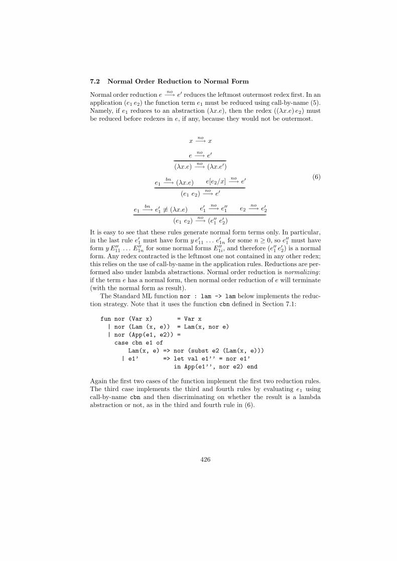
7.2 Normal Order Reduction to Normal Form

Normal order reduction eno−→ e′ reduces the leftmost outermost redex first. In an

application (e1 e2) the function term e1 must be reduced using call-by-name (5).Namely, if e1 reduces to an abstraction (λx.e), then the redex ((λx.e) e2) mustbe reduced before redexes in e, if any, because they would not be outermost.

xno−→ x

eno−→ e′

-------------------------------------------------------------------------------(λx.e)

no−→ (λx.e′)

e1bn−→ (λx.e) e[e2/x]

no−→ e′

-----------------------------------------------------------------------------------------------------------------------------------------(e1 e2)

no−→ e′

e1bn−→ e′1 6≡ (λx.e) e′1

no−→ e′′1 e2

no−→ e′2

--------------------------------------------------------------------------------------------------------------------------------------------------------------------------------------------------------(e1 e2)

no−→ (e′′1 e′2)

(6)

It is easy to see that these rules generate normal form terms only. In particular,in the last rule e′1 must have form y e′11 . . . e′1n for some n ≥ 0, so e′′1 must haveform y E′′

11 . . . E′′

1n for some normal forms E ′′

1i, and therefore (e′′1 e′2) is a normalform. Any redex contracted is the leftmost one not contained in any other redex;this relies on the use of call-by-name in the application rules. Reductions are per-formed also under lambda abstractions. Normal order reduction is normalizing :if the term e has a normal form, then normal order reduction of e will terminate(with the normal form as result).

The Standard ML function nor : lam -> lam below implements the reduc-tion strategy. Note that it uses the function cbn defined in Section 7.1:

fun nor (Var x) = Var x

| nor (Lam (x, e)) = Lam(x, nor e)

| nor (App(e1, e2)) =

case cbn e1 of

Lam(x, e) => nor (subst e2 (Lam(x, e)))

| e1’ => let val e1’’ = nor e1’

in App(e1’’, nor e2) end

Again the first two cases of the function implement the first two reduction rules.The third case implements the third and fourth rules by evaluating e1 usingcall-by-name cbn and then discriminating on whether the result is a lambdaabstraction or not, as in the third and fourth rule in (6).

426

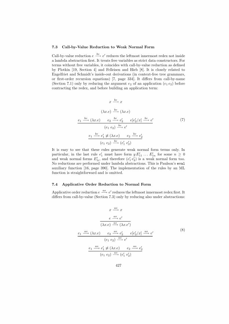
7.3 Call-by-Value Reduction to Weak Normal Form

Call-by-value reduction ebv−→ e′ reduces the leftmost innermost redex not inside

a lambda abstraction first. It treats free variables as strict data constructors. Forterms without free variables, it coincides with call-by-value reduction as definedby Plotkin [19, Section 4] and Felleisen and Hieb [8]. It is closely related toEngelfriet and Schmidt’s inside-out derivations (in context-free tree grammars,or first-order recursion equations) [7, page 334]. It differs from call-by-name(Section 7.1) only by reducing the argument e2 of an application (e1 e2) beforecontracting the redex, and before building an application term:

xbv−→ x

(λx.e)bv−→ (λx.e)

e1bv−→ (λx.e) e2

bv−→ e′2 e[e′2/x]

bv−→ e′

----------------------------------------------------------------------------------------------------------------------------------------------------------------------------------------------------(e1 e2)

bv−→ e′

e1bv−→ e′1 6≡ (λx.e) e2

bv−→ e′2--------------------------------------------------------------------------------------------------------------------------------------------

(e1 e2)bv−→ (e′1 e′2)

(7)

It is easy to see that these rules generate weak normal form terms only. Inparticular, in the last rule e′1 must have form y E′

11 . . . E′

1n for some n ≥ 0and weak normal forms E ′

1i, and therefore (e′1 e′2) is a weak normal form too.No reductions are performed under lambda abstractions. This is Paulson’s evalauxiliary function [16, page 390]. The implementation of the rules by an MLfunction is straightforward and is omitted.

7.4 Applicative Order Reduction to Normal Form

Applicative order reduction eao−→ e′ reduces the leftmost innermost redex first. It

differs from call-by-value (Section 7.3) only by reducing also under abstractions:

xao−→ x

eao−→ e′

-------------------------------------------------------------------------------(λx.e)

ao−→ (λx.e′)

e1ao−→ (λx.e) e2

ao−→ e′2 e[e′2/x]

ao−→ e′

----------------------------------------------------------------------------------------------------------------------------------------------------------------------------------------------------(e1 e2)

ao−→ e′

e1ao−→ e′1 6≡ (λx.e) e2

ao−→ e′2--------------------------------------------------------------------------------------------------------------------------------------------

(e1 e2)ao−→ (e′1 e′2)

(8)

427

It is easy to see that the rules generate only normal form terms. As before, notethat in the last rule e′1 must have form y E′

11 . . . E′

1n for some n ≥ 0 and normalforms E′

1i. Also, it is clear that when a redex ((λx.e) e′2) is contracted, it containsno other redex, and it is the leftmost redex with this property.

Applicative order reduction is not normalizing; with Ω ≡ (λx.(x x))(λx.(x x))it produces an infinite reduction ((λx.y) Ω) −→β ((λx.y) Ω) −→β . . . althoughthe term has normal form y.

In fact, applicative order reduction fails to normalize applications of functionsdefined using recursion combinators, even with recursion combinators designedfor call-by-value, such as Yv :

Yv ≡ λh.(λx.λa.h (x x) a) (λx.λa.h (x x) a) (9)

7.5 Hybrid Applicative Order Reduction to Normal Form

Hybrid applicative order reduction is a hybrid of call-by-value and applicativeorder reduction. It reduces to normal form, but reduces under lambda abstrac-tions only in argument positions. Therefore the usual call-by-value versions ofthe recursion combinator, such as (9) above, may be used with this reductionstrategy. Thus the hybrid applicative order strategy normalizes more terms thanapplicative order reduction, while using fewer reduction steps than normal orderreduction. The hybrid applicative order strategy relates to call-by-value in thesame way that the normal order strategy relates to call-by-name. It resemblesPaulson’s call-by-value strategy, which works in two phases: first reduce the term

bybv−→ , then normalize the bodies of any remaining lambda abstractions [16,

page 391].

xha−→ x

eha−→ e′

-------------------------------------------------------------------------------(λx.e)

ha−→ (λx.e′)

e1bv−→ (λx.e) e2

ha−→ e′2 e[e′2/x]

ha−→ e′

----------------------------------------------------------------------------------------------------------------------------------------------------------------------------------------------------(e1 e2)

ha−→ e′

e1bv−→ e′1 6≡ (λx.e) e′1

ha−→ e′′1 e2

ha−→ e′2--------------------------------------------------------------------------------------------------------------------------------------------------------------------------------------------------------

(e1 e2)ha−→ (e′′1 e′2)

(10)

428

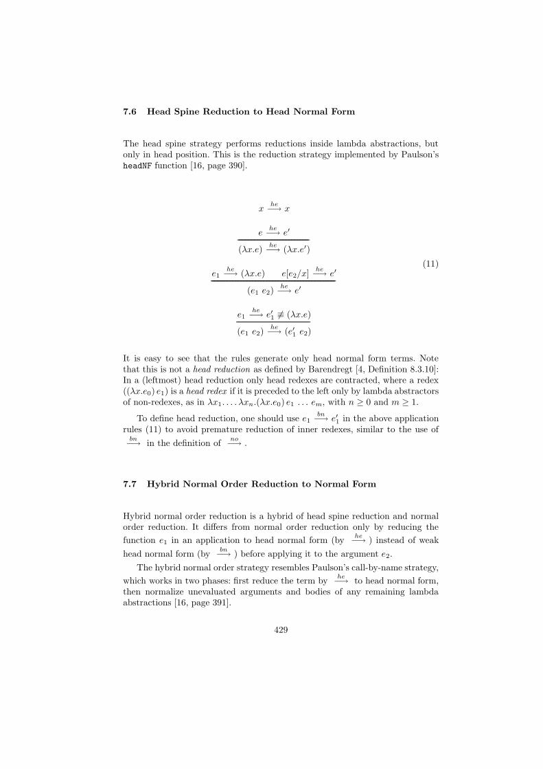
7.6 Head Spine Reduction to Head Normal Form

The head spine strategy performs reductions inside lambda abstractions, butonly in head position. This is the reduction strategy implemented by Paulson’sheadNF function [16, page 390].

xhe−→ x

ehe−→ e′

-------------------------------------------------------------------------------(λx.e)

he−→ (λx.e′)

e1he−→ (λx.e) e[e2/x]

he−→ e′

-----------------------------------------------------------------------------------------------------------------------------------------(e1 e2)

he−→ e′

e1he−→ e′1 6≡ (λx.e)

---------------------------------------------------------------------------------(e1 e2)

he−→ (e′1 e2)

(11)

It is easy to see that the rules generate only head normal form terms. Notethat this is not a head reduction as defined by Barendregt [4, Definition 8.3.10]:In a (leftmost) head reduction only head redexes are contracted, where a redex((λx.e0) e1) is a head redex if it is preceded to the left only by lambda abstractorsof non-redexes, as in λx1. . . . λxn.(λx.e0) e1 . . . em, with n ≥ 0 and m ≥ 1.

To define head reduction, one should use e1bn−→ e′1 in the above application

rules (11) to avoid premature reduction of inner redexes, similar to the use ofbn−→ in the definition of

no−→ .

7.7 Hybrid Normal Order Reduction to Normal Form

Hybrid normal order reduction is a hybrid of head spine reduction and normalorder reduction. It differs from normal order reduction only by reducing the

function e1 in an application to head normal form (byhe−→ ) instead of weak

head normal form (bybn−→ ) before applying it to the argument e2.

The hybrid normal order strategy resembles Paulson’s call-by-name strategy,

which works in two phases: first reduce the term byhe−→ to head normal form,

then normalize unevaluated arguments and bodies of any remaining lambdaabstractions [16, page 391].

429

xhn−→ x

ehn−→ e′

-------------------------------------------------------------------------------(λx.e)

hn−→ (λx.e′)

e1he−→ (λx.e) e[e2/x]

hn−→ e′

-----------------------------------------------------------------------------------------------------------------------------------------(e1 e2)

hn−→ e′

e1he−→ e′1 6≡ (λx.e) e′1

hn−→ e′′1 e2

hn−→ e′2--------------------------------------------------------------------------------------------------------------------------------------------------------------------------------------------------------

(e1 e2)hn−→ (e′′1 e′2)

(12)

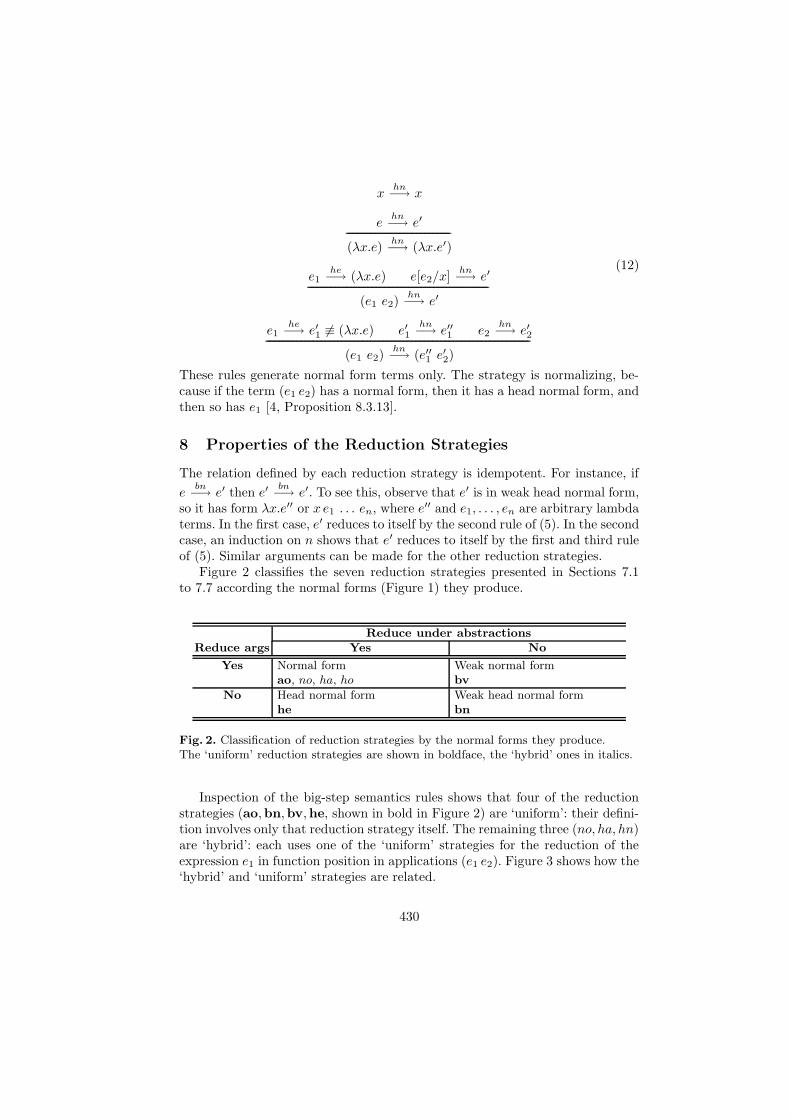
These rules generate normal form terms only. The strategy is normalizing, be-cause if the term (e1 e2) has a normal form, then it has a head normal form, andthen so has e1 [4, Proposition 8.3.13].

8 Properties of the Reduction Strategies

The relation defined by each reduction strategy is idempotent. For instance, if

ebn−→ e′ then e′

bn−→ e′. To see this, observe that e′ is in weak head normal form,

so it has form λx.e′′ or x e1 . . . en, where e′′ and e1, . . . , en are arbitrary lambdaterms. In the first case, e′ reduces to itself by the second rule of (5). In the secondcase, an induction on n shows that e′ reduces to itself by the first and third ruleof (5). Similar arguments can be made for the other reduction strategies.

Figure 2 classifies the seven reduction strategies presented in Sections 7.1to 7.7 according the normal forms (Figure 1) they produce.

Reduce under abstractions

Reduce args Yes No

Yes Normal formao, no, ha, ho

Weak normal formbv

No Head normal formhe

Weak head normal formbn

Fig. 2. Classification of reduction strategies by the normal forms they produce.The ‘uniform’ reduction strategies are shown in boldface, the ‘hybrid’ ones in italics.

Inspection of the big-step semantics rules shows that four of the reductionstrategies (ao,bn,bv,he, shown in bold in Figure 2) are ‘uniform’: their defini-tion involves only that reduction strategy itself. The remaining three (no, ha, hn)are ‘hybrid’: each uses one of the ‘uniform’ strategies for the reduction of theexpression e1 in function position in applications (e1 e2). Figure 3 shows how the‘hybrid’ and ‘uniform’ strategies are related.

430

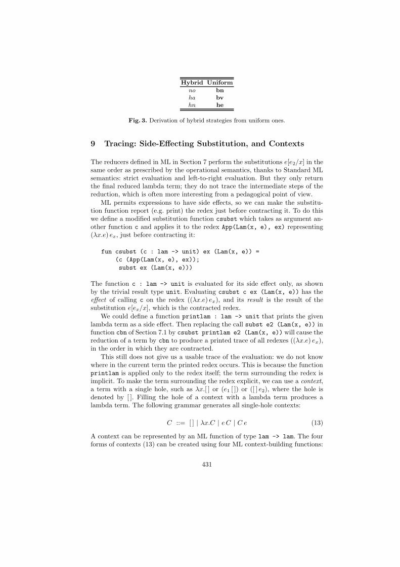
Hybrid Uniform

no bn

ha bv

hn he

Fig. 3. Derivation of hybrid strategies from uniform ones.

9 Tracing: Side-Effecting Substitution, and Contexts

The reducers defined in ML in Section 7 perform the substitutions e[e2/x] in thesame order as prescribed by the operational semantics, thanks to Standard MLsemantics: strict evaluation and left-to-right evaluation. But they only returnthe final reduced lambda term; they do not trace the intermediate steps of thereduction, which is often more interesting from a pedagogical point of view.

ML permits expressions to have side effects, so we can make the substitu-tion function report (e.g. print) the redex just before contracting it. To do thiswe define a modified substitution function csubst which takes as argument an-other function c and applies it to the redex App(Lam(x, e), ex) representing(λx.e) ex, just before contracting it:

fun csubst (c : lam -> unit) ex (Lam(x, e)) =

(c (App(Lam(x, e), ex));

subst ex (Lam(x, e)))

The function c : lam -> unit is evaluated for its side effect only, as shownby the trivial result type unit. Evaluating csubst c ex (Lam(x, e)) has theeffect of calling c on the redex ((λx.e) ex), and its result is the result of thesubstitution e[ex/x], which is the contracted redex.

We could define a function printlam : lam -> unit that prints the givenlambda term as a side effect. Then replacing the call subst e2 (Lam(x, e)) infunction cbn of Section 7.1 by csubst printlam e2 (Lam(x, e)) will cause thereduction of a term by cbn to produce a printed trace of all redexes ((λx.e) ex),in the order in which they are contracted.

This still does not give us a usable trace of the evaluation: we do not knowwhere in the current term the printed redex occurs. This is because the functionprintlam is applied only to the redex itself; the term surrounding the redex isimplicit. To make the term surrounding the redex explicit, we can use a context,a term with a single hole, such as λx.[ ] or (e1 [ ]) or ([ ] e2), where the hole isdenoted by [ ]. Filling the hole of a context with a lambda term produces alambda term. The following grammar generates all single-hole contexts:

C ::= [ ] | λx.C | e C | C e (13)

A context can be represented by an ML function of type lam -> lam. The fourforms of contexts (13) can be created using four ML context-building functions:

431

fun id e = e

fun Lamx x e = Lam(x, e)

fun App2 e1 e2 = App(e1, e2)

fun App1 e2 e1 = App(e1, e2)

For instance, (App1 e2) is the ML function fn e1 => App(e1, e2) which rep-resents the context ([ ] e2). Filling the hole with the term e1 is done by computing(App1 e2) e1 which evaluates to App(e1, e2), representing the term (e1 e2).

Function composition (f o g) composes contexts. For instance, the compo-sition of contexts λx.[ ] and ([ ] e2) is Lamx x o App1 e2, which represents thecontext λx.([ ] e2). Similarly, the composition of the contexts ([ ] e2) and λx.[ ] isApp1 e2 o Lamx x, which represents ((λx.[ ]) e2).

10 Reduction in Context

To produce a trace of the reduction, we modify the reduction functions definedin Section 7 to take an extra context argument c and to use the extended sub-stitution function csubst, passing c to csubst. Then csubst will apply c to theredex before contracting it. We take the call-by-name reduction function cbn

(Section 7.1) as an example; the other reduction functions are handled similarly.The reduction function must build up the context c as it descends into the term.It does so by composing the context with the appropriate context builder (inthis case, only in the App branch):

fun cbnc c (Var x) = Var x

| cbnc c (Lam(x, e)) = Lam(x, e)

| cbnc c (App(e1, e2)) =

case cbnc (c o App1 e2) e1 of

Lam (x, e) => cbnc c (csubst c e2 (Lam(x, e)))

| e1’ => App(e1’, e2)

By construction, if c : lam -> lam and the evaluation of cbnc c e involves acall cbnc c′ e′, then c[e] −→∗

β c′[e′]. Also, whenever a call cbnc c′ (e1 e2) is

evaluated, and e1bn−→ (λx.e), then function c′ is applied to the redex ((λx.e) e2)

just before it is contracted. Hence a trace of the reduction of term e can beobtained just by calling cbnc as follows:

cbnc printlam e

where printlam : lam -> unit is a function that prints the lambda term asa side effect. In fact, computing cbnc printlam (App (App add two) two),using the encodings from (1), prints the two intermediate terms below. Thethird term shown is the final result (a weak head normal form):

(\m.\n.\f.\x.m f (n f x)) (\f.\x.f (f x)) (\f.\x.f (f x))

(\n.\f.\x.(\f.\x.f (f x)) f (n f x)) (\f.\x.f (f x))

\f.\x.(\f.\x.f (f x)) f ((\f.\x.f (f x)) f x)

432

The trace of a reduction can be defined also by direct instrumentation of theoperational semantics (5). Let us define a trace to be a finite sequence of lambdaterms, denote the empty trace by ε, and denote the concatenation of traces s

and t by s · t. Now we define the relation ebn−→

s

C e′ to mean: under call-by-name,the expression e reduces to e′, and if e appears in context C, then s is the traceof the reduction. The trace s will be empty if no redex was contracted in thereduction. If some redex was contracted, the first term in the trace will be e.

The tracing relation corresponding to call-by-name reduction (5) can be de-fined as shown below:

xbn−→

ε

C x

(λx.e)bn−→

ε

C (λx.e)

e1bn−→

s

C[[ ] e2] (λx.e) e[e2/x]bn−→

t

C e′--------------------------------------------------------------------------------------------------------------------------------------------------------------------------

(e1 e2)bn−→

s·C[(λx.e) e2]·t

C e′

e1bn−→

s

C[[ ] e2] e′1 6≡ λx.e---------------------------------------------------------------------------------------------------

(e1 e2)bn−→

s

C (e′1 e2)

(14)

Thus reduction of a variable x or a lambda abstraction (λx.e) produces the emptytrace ε. When e1 reduces to a lambda abstraction, reduction of the application(e1 e2) produces the trace s · C[(λx.e) e2] · t, where s traces the reduction of e1

and t traces the reduction of the contracted redex e[e2/x].Tracing versions of the other reduction strategies can be defined analogously.

11 Single-Stepping Reduction

For experimentation it is useful to be able to perform one beta-reduction at atime, or in other words, to single-step the reduction. Again, this can be achievedusing side effects in the implementation language. We simply make the contextfunction c count the number of redexes contracted (substitutions performed),and set a step limit N before evaluation is started.

When N redexes have been contracted, c aborts the reduction by raising anexception Enough e′, which carries as its argument the term e′ that had beenobtained after N reductions. An enclosing exception handler returns e′ as theresult of the reduction. The next invocation of the reduction function simplysets the step limit N one higher, and so on. Thus the reduction of the originalterm starts over for every new step, but we create the illusion of reducing theterm one step at a time.

The main drawback of this approach is that the total time spent performingn steps of reduction is O(n2). In practice, this does not matter: noboby wantsto single-step very long computations.

433

12 A Web-Based Interface to the Reduction Functions

A web-based interface to the tracing reduction functions can be implemented asan ordinary CGI script. The lambda term to be reduced, the name of the desiredreduction strategy, the kind of computation (tracing, single-stepping, etc.) andthe step limit are passed as parameters to the script.

Such an implementation has been written in Moscow ML [15] and is availableat 〈http://www.dina.kvl.dk/˜sestoft/lamreduce/〉. The implementation uses theMosmlcgi library to access CGI parameters, and the Msp library for efficientstructured generation of HTML code.

For tracing, the script uses a function htmllam : lam -> unit that printsa lambda term as HTML code, which is then sent to the browser by the webserver. Calling cbnc (or any other tracing reduction function) with htmllam asargument will display a trace of the reduction in the browser.

A trick is used to make the next redex into a hyperlink in the browser.The implementation’s representation of lambda terms is extended with labelledsubterms, and csubst attaches labels 0, 1, . . . to redexes in the order in whichthey are contracted. When single-stepping a reduction, the last labelled redexinside the term can be formatted as a hyperlink. Clicking on the hyperlink willcall the CGI script again to perform one more step of reduction, creating theillusion of single-stepping the reduction as explained above.

13 Conclusion

We have described a simple way to implement lambda calculus reduction, de-scribing reduction strategies using big-step operational semantics, implementingreduction by straightforward reduction functions in Standard ML, and instru-menting them to produce a trace of the reduction, using contexts. This approachis easily extended to other reduction strategies describable by big-step opera-tional semantics.

We find that big-step semantics provides a clear presentation of the reductionstrategies, highlighting their differences and making it easy to see what normalforms they produce.

The extension to lazy evaluation, whether using graph reduction or an explicitheap, would be complicated mostly by the need to represent the current termgraph or heap, and to print it in a comprehensible way.

The functions for reduction in context were useful for creating a web inter-face also, running the reduction functions as a CGI script written in ML. Theweb interface provides a simple platform for students’ experiments with lambdacalculus encodings and reduction strategies.

Acknowledgements Thanks for Dave Schmidt for helpful comments that haveimproved contents as well as presentation.

434

References

1. Abramsky, S., Ong, C.-H.L.: Full Abstraction in the Lazy λ-Calculus. Informationand Computation 105, 2 (1993) 159–268.

2. Ariola, Z.M., Felleisen, M.: The Call-by-Need Lambda Calculus. Journal of Func-tional Programming 7, 3 (1997) 265–301.

3. Augustsson, L.: A Compiler for Lazy ML. In: 1984 ACM Symposium on Lisp andFunctional Programming, Austin, Texas. ACM Press (1984) 218–227.

4. Barendregt, H.P.: The Lambda Calculus. Its Syntax and Semantics. North-Holland(1984).

5. Barendregt, H.P. et al.: Needed Reduction and Spine Strategies for the LambdaCalculus. Information and Computation 75 (1987) 191–231.

6. Church, A.: A Note on the Entscheidungsproblem. Journal of Symbolic Logic 1

(1936) 40–41, 101–102.7. Engelfriet, J., Schmidt, E.M.: IO and OI. Journal of Computer and System Sciences

15 (1977) 328–353 and 16 (1978) 67–99.8. Felleisen, M., Hieb, R.: The Revised Report on the Syntactic Theories of Sequential

Control and State. Theoretical Computer Science 103, 2 (1992) 235–271.9. Kahn, G.: Natural Semantics. In: STACS 87. 4th Annual Symposium on Theoret-

ical Aspects of Computer Science, Passau, Germany. Lecture Notes in ComputerScience, Vol. 247. Springer-Verlag (1987) 22–39.

10. Landin, P.J.: The Mechanical Evaluation of Expressions. Computer Journal 6, 4(1964) 308–320.

11. Landin, P.J.: A Correspondence Between ALGOL 60 and Church’s Lambda-Notation: Part I. Communications of the ACM 8, 2 (1965) 89–101.

12. Landin, P.J.: The Next 700 Programming Languages. Communications of the ACM9, 3 (1966) 157–166.

13. Launchbury, J.: A Natural Semantics for Lazy Evaluation. In: Twentieth ACMSymposium on Principles of Programming Languages, Charleston, South Carolina,January 1993. ACM Press (1993) 144–154.

14. Milner, R., Tofte, M., Harper, R., MacQueen, D.B.: The Definition of StandardML (Revised). The MIT Press (1997).

15. Moscow ML is available at 〈http://www.dina.kvl.dk/˜sestoft/mosml.html〉.16. Paulson, L.C.: ML for the Working Programmer. Second edition. Cambridge Uni-

versity Press (1996).17. Peyton Jones, S.L.: The Implementation of Functional Programming Languages.

Prentice-Hall (1987).18. Peyton Jones, S.L., Hughes, J. (eds.): Haskell 98: A Non-Strict, Purely Functional

Language. At 〈http://www.haskell.org/onlinereport/〉.19. Plotkin, G.: Call-by-Name, Call-by-Value and the λ-Calculus. Theoretical Com-

puter Science 1 (1975) 125–159.20. Revised4 Report on the Algorithmic Language Scheme, IEEE Std 1178-1990. In-

stitute of Electrical and Electronic Engineers (1991).21. Sestoft, P.: Deriving a Lazy Abstract Machine. Journal of Functional Programming

7, 3 (1997) 231–264.22. Stoy, J.E.: The Scott-Strachey Approach to Programming Language Theory. The

MIT Press (1977).23. Turner, D.A.: A New Implementation Technique for Applicative Languages. Soft-

ware – Practice and Experience 9 (1979) 31–49.24. Wadsworth, C.P.: Semantics and Pragmatics of the Lambda Calculus. D.Phil. the-

sis, Oxford University, September 1971.

435