demand side management in the smart grid - … · demand side management in the smart grid pr esent...
TRANSCRIPT

UNIVERSITE DE MONTREAL
DEMAND SIDE MANAGEMENT IN THE SMART GRID
GIUSEPPE TOMMASO COSTANZO
DEPARTEMENT DE GENIE ELECTRIQUE
ECOLE POLYTECHNIQUE DE MONTREAL
MEMOIRE PRESENTE EN VUE DE L’OBTENTION
DU DIPLOME DE MAITRISE ES SCIENCES APPLIQUEES
(GENIE ELECTRIQUE)
NOVEMBRE 2011
c© Giuseppe Tommaso Costanzo, 2011.

UNIVERSITE DE MONTREAL
ECOLE POLYTECHNIQUE DE MONTREAL
Ce memoire intitule:
DEMAND SIDE MANAGEMENT IN THE SMART GRID
presente par: COSTANZO, Giuseppe Tommaso
en vue de l’obtention du diplome de: Maıtrise es Sciences Appliquees
a ete dument accepte par le jury d’examen constitue de:
M. MALHAME, Roland, Ph.D., president
M. ZHU, Guchuan, Doct., membre et directeur de recherche
M. ANJOS, Miguel F., Ph.D., membre et codirecteur de recherche
M. SAVARD, Gilles, Ph.D., membre

iii
A mes tres cher grand parents
Angela, Tomaso et Giuseppe
qui n’ont pas vecu assex pour voir ce memoire.

iv
ACKNOWLEDGEMENTS
I would like to express my sincere gratitude to my research directors Prof. Guchuan Zhu
at Ecole Polytechnique de Montreal, Prof. Luca Ferrarini at Politecnico di Milano and my
research codirector Prof. Miguel F. Anjos at Ecole Polytechnique de Montreal for their
continuous guidance, suggestions and essential encouragement during my graduate studies.
The experimental study presented in this thesis have been supported by DERri (Dis-
tributed Energy Resource Research Infrastructure as a part of a collaboration between Po-
litecnico di Milano and DTU - Danish Technical University. The author is particularly
grateful to the staff of the Intelligent Energy Systems department of RISØ DTU for not only
the precious help and advice during the experiments, but also for a great hospitality.
These last two years in Montreal have been so dense of experiences and so many people
left their footprint in my memories that I wish everyone could have such privilege like I had.
Particularly, thank you Annick for your precious advice upon my arrival and during my
studies in Montreal, Matti and Ire for your essential contribution in the composition and
revision of the French summary, Melanie, Ramin, Sean, Nicolette and Heather for proof-
reding my english.
Thank you Amir, my Iranian brother, for being the best roomate ever and most sincere
friend.
Thanks to my university collegues and friends, such stressing studies have turned into
the most enjoyable and amazing adventure: Hani, Jean-Philippe, Sergio, Davide, Matthew,
Jacopo, Francesca, Kayla, Paula, Cecilia. Thank you Jan for your friendship and relevant
contribution in our first conference paper, you’re a brilliant engineer and the most hard-
working collegue I had!
Thank you Jessica and Roberto for sharing with me your passion for Tango and teaching
me such marvellous dance and life style.
Thank you my collegues alcooliques Eddy and Lucas, and all the AECSP group for the
uncountable parties and outgoings together.
Finally, and most importantly, I am deeply grateful to my beloved family for always loving,
encouraging and supporting me: my parents Luciano and Enza, my little sister Angela and
my grandmother Lina.
I address a special thought to my grandparents Tomaso, Angela and Giuseppe, whose
humanity, honesty and love for culture have always been for me reference points.

v
RESUME
L’objectif du present projet est de developper des solutions pour ameliorer l’efficacite energetique
dans les reseaux electriques. L’approche adoptee dans cette recherche est basee sur un con-
cept nouveau dans le Smart Grids (reseaux electriques intelligents), l’optimisation du De-
mand/Response, qui permet la mise en œuvre de la gestion autonome de la demande de
energie pour une grande variete de consommateurs, des les maisons a les batiments, usines,
centres commerciaux, les campus, les bases militaires, et meme les micro-reseaux.
La premiere partie de cette these presente le theme de la Smart Grid et evalue l’etat de l’art
par rapport aux portees du projet. Ensuite, nous introduisons une architecture pour la gestion
autonome de la charge du cote de la demande. Cette architecture est composee par trois
couches principales, dont deux, l’ordonnancement en ligne et l’ordonnancement au moindre
cout, sont pleinement pris en compte, tandis que la troisieme couche, la Demande/Response,
est laisse comme une extension future. Une telle architecture tire profit de la separation
des des echelles de temps de la consommation d’energie, et elle est evolutif et flexible. La
deuxieme partie de ce projet est axe sur la mise en œuvre de l’architecture proposee dans
Matlab/Simulink, apres une preuve de concept est donnee par des simulations et resultats
experimentaux.
Mots-cles: programmation optimale de la charge, nivelement de la charge de pointe,
Demand-Side Management (DSM) autonome, batiments intelligents, Demand/Response, ef-
ficacite energetique.

vi
ABSTRACT
The objective of the present project is to develop solutions to improve energy efficiency in
electric grids. The basic approach adopted in this research is based on a new concept in the
Smart Grid, namely Demand/Response Optimization, which enables the implementation of
the autonomous demand side energy management for a big variety of consumers, ranging
from homes to buildings, factories, commercial centers, campuses, military bases, and even
micro-grids.
The first part of this thesis presents the topic of the Smart Grid and assesses the state
of the art with respect to the scopes of the project. Afterward, we introduce an architecture
for autonomous demand side load management composed of three main layers, of which two,
online scheduling and minimum-cost scheduling, are fully addressed, while the third layer,
Demand/Response, is left as future extension. Such architecture takes advantage of time-
scale separation of energy consumption. It is scalable and flexible. The second part of this
project is focused on the implementation of the proposed architecture in Matlab/Simulink
and a proof of concept is given through simulations and experimental results.
Keywords: Optimal load scheduling, Peak-load shaving, Autonomous Demand-Side Man-
agement (DSM), Smart Buildings, Demand/Response, Energy efficiency.

vii
CONDENSE EN FRANCAIS
Introduction
Le reseau electrique intelligent (the Smart Grid) est une technologie emergente dans le do-
maine des systemes de production, transmission et utilisation de l’energie. Ceci aura un
impact profond sur la vie de nombreux consommateurs au cours de ce siecle. Les progres
dans ce domaine apporteront egalement de multiples avantages economiques, sociaux et en-
vironnementaux dans notre societe. Pour faire face a ce defi, non seulement la communaute
scientifique mais aussi de nombreux partenaires industriels et publics prennent des mesures
pour moderniser les infrastructures du reseau electrique et des technologies connexes, afin
d’assurer la production et la distribution d’energie dans le siecle prochain.
Cette recherche a pour but d’apporter des instruments pour une gestion efficace de
l’energie electrique, qui peut etre etendue a differents niveaux de la Smart Grid (comme
a la maison, dans le batiment ou le district). Ce travail se concentre en particulier sur
l’optimisation des charges electrique de consommateurs en vue de favoriser l’utilisation des
sources renouvelables dans les reseaux de distribution et de permettre une consommation
intelligente de l’energie.
Les Reseaux Electriques Inteligents
D’apres la definition de F.L. Bellifemine, le Smart Grid est “un reseau electrique capable
d’integrer toutes les actions des clients et des producteurs branches au fin de distribuer
l’energie electrique de maniere efficace, durable, a bas prix et en toute securite.”[Bellifemine,
F.L. et al. (2009)]. Le mot Smart Grid exprime “une vision combinee qui utilise le reseau
d’information pour ameliorer le fonctionnement du reseau d’electricite.”[V. Pothamsetty and
S. Malik (February 2009)].
Par rapport aux reseaux electriques traditionnels, la Smart Grid peut gerer des flux bidi-
rectionnels d’electricite et d’information. Cette caracteristique joue un role cle pour une
participation active des consommateurs dans le marche energetique. L’union entre les infras-
tructures du reseau electrique et des technologies disponibles dans le domaine des commu-
nications permettra la programmation de la consommation, la prevision de charge et le niv-
ellement des pics de charge dans le reseau de distribution ce qui ameliorera considerablement
l’efficacite du reseau.
Le controle des charges du consommateur et son interfacage vers la grille visent a une
amelioration de l’efficacite energetique. Les sujets d’interet de ce domaine comprennent:

viii
• Compteurs intelligents: appareils capables de mesurer des grandeurs differentes en
temps reel, d’analyser les donnees et de les rapporter grace a des systemes de commu-
nication. Ces dispositifs peuvent etre integres dans une structure de mesure avancee
(Advanced Metering Infrastructure) qui fournit des types d’informations differents et
de services pour les clients et les fournisseurs d’energie.
• Appareils intelligents et domotique: ce secteur concerne la modernisation des appareils
electromenagers afin de communiquer et ajuster leur fonctionnement aux besoins des
usagers en vue d’optimiser la consommation electrique.
• Gestion dynamique et prevision des consommations: ceci permettrait aux clients une
meilleure programmation des activites a domicile dependament du prix de l’energie.
Pour les fournisseurs, en revanche, cette gestion serait extremement utile pour l’optimisation
de la production de l’energie.
• Integration et optimisation des sources d’energie renouvelables: l’augmentation des cen-
trales de generation distribuee et la forte penetration des ressources renouvelables dans
le marchee energetique, represente un grand defi pour l’augmentation de la stabilite
du reseau et de l’efficacite ainsi que la baisse des emissions de CO2. Par ailleurs, la
participation des clients dans le marche energetique a travers la cooperation des pays,
l’integration des nouvelles technologies, la standardisation, l’augmentation de fiabilite
et les nouveaux investissements dans les pays de l’Union Europeenne et de l’Amerique
du Nord sont facteurs importants pour la construction des Smart Grids.
• Optimisation du “demand/response” et la tarification dynamique de l’energie, qui per-
mettra un controle intelligent des charges selon le prix de l’energie. De cette maniere
les clients peuvent regler leurs consommations en temps reel selon le tarif.
• Cyber securite: aujourd’hui les reseaux electriques peuvent offrir un bon niveau de
securite informatique contre les attaques des pirates informatiques grace a des standards
et des reseaux de communication dedies, ainsi que des systemes de controle redondantes.
Il ne reste qu’a verifier si le passage au Smart Grid rendra les pays plus vulnerables
aux attaques informatiques.
Une architecture pour la gestion automatisee de la charge electrique
La distribution intelligente de l’energie serait une application directe des compteurs intel-
ligents. Ces premiers permettront une consommation optimisee en coordonnant tous les
dispositifs afin de minimiser les couts. Commerce et tarification de l’energie en temps reel,

ix
choix eco durables, gestion du CO2, ne sont que quelques applications possibles dans le
domaine de l’automatisation des batiments.
L’architecture du systeme propose pour le DSM (Demand Side Management) consiste
en trois niveaux principaux (figure 0.1): Admission Control (AC), Load Balancing (LB)
et Demand/ Response Manager (DRM). AC est le niveau inferieur qui interagit avec les
appareils intelligents pour le controle de la consommation en temps reel. Dans ce travail,
l’approche adoptee pour le controle des appareils utilise des strategies de planification en
ligne inspiree de la technique d’ordonnancement dans les systemes informatiques embarques
(voir, par exemple, [Buttazzo (2005)] et les references citees).
L’introduction d’un modele d’appareil electromenage generique permet la planification
des activites et de la consommation de facon systematique. Le niveau superieur, le DRM,
est l’entree du systeme DSM et represente une interface a la Smart Grid. Il est possible de
mettre au point plusieurs strategies de tarification de l’energie comme la tarification de pointe
critique ou la tarification de temps d’utilisation. Le niveau intermediaire (LB) coordonne les
activites du niveau superieur (DRM) et inferieur (AC) et equilibre la consommation a travers
un algorithme qui repartit la charge en minimisant les couts energetiques. L’equilibrage
de charge entraıne un probleme d’optimisation qui sera resolu avec les instruments de la
programmation lineaire. Le LB fournit egalement au DRM des informations importantes
concernant le taux de rejet des demandes, un parametre de performance requis pour la
gestion effective du Demand/Response. Les charges electriques sont classees selon leurs
caracteristiques intrinseques en trois categories differentes:
1. La charge de base est une consommation electrique requise necessaire des appareils
qui sont actives immediatement a n’importe quel moment ou pour le maintien dans
l’etat de “stand by”. Cette categorie comprend l’eclairage, les ordinateurs, les systemes
de communication et tous les autres dispositifs dont la valeur commerciale ne permet
pas l’installation d’une intelligence comme le seche cheveux, le toaster ou le chargeur.
2. La charge reguliere est la puissance requise par les electromenagers qui sont toujours
en fonction pendant une longue periode de temps, comme la climatisation, le chauffage
ou le refrigerateur.
3. La charge de pointe est propre aux appareils dont le cycle d’operation a une duree
fixe. Cette categorie comprend, par exemple, le seche linge, le lave-vaisselle, la machine
a laver ou le four. Souvent les pics d’absorption sont causees par l’accumulation des
charges de pointe avec des charges regulieres. Par consequent, une gestion attentive de
la charge de pointe devient fondamentale pour la reduction des couts de l’energie.

x
Load Balancer
D/R
Manager
Load
Forecaster
REQUEST
REJECT
ACCEPT
Consumption
Information
Available
Capacity
Predicted
Demand
Burst Load
Smart Grid
Smart Grid Interface
DSM SystemCapacity/Price
Regular Load
Schedule
Admission Controller
Capacity Limit
Baseline Load
Predicted
Load
Ap
plia
nce
In
terf
ace
Sm
art
Me
ter
Figure 0.1 Architecture propose pour le systeme de gestion des charges.
Dans cette recherche, les appareils electromenagers intelligents sont supposes etre capables
de communiquer avec le gestionaire d’energie et de garantir un controle adequat au niveau
des dispositifs. La communication au sein du systeme DSM doit etre suffisamment fiable et
les retards doivent etre negligeables par rapport a la dynamique des appareils. Le reseau
de communication se base sur des technologies filaires et sans fil [Drake et al. (2010),Li et
Sun (2010)] et utilise des interfaces speciales pour communiquer avec les electromenagers
intelligents.
Une telle architecture se base sur la division temporelle des dynamiques liees a la gestion
des charges domestiques.
Mise en œuvre avec Matlab/Simulink
Cette section presente la mise en œuvre de l’architecture proposee avec Matlab/Simulink,
ainsi que des etudes de simulation pour le systeme de gestion des charges residentielles. Le
schema Simulink du systeme envisage est montre dans la figure 0.2, ou chaque composant peut
etre facilement identifie dans l’architecture presentee a la section du DSM (sec. 3.2). Notez
que, meme si dans la simulation les appareils sont representes par des modeles simplifies,
l’architecture proposee dans cette recherche est concue independamment de la precision du

xi
modele des appareils. Les performances de la gestion de la charge dans l’implementation
reelle seront effectivement influencees par les modeles des appareils. La periode de simulation
1act_signals
Out
1
triggerrej_rate
Scope2
uapp
basfcn
SIGNAL SPLITTER
New_Schedule
C_used
Updated_Schedule
SCHED. MANAGER
signals
schedule
requestsrequestgen
REQUESTSGENERATOR
Memory1 Memory 2
Memory
Rejected
Requests
Cprof ile
Schedule
Energy cost prof ile
Out_Schedule
Load Balancer
BSL
Goto
activ e
schedule
act
opdispatcher
DISPATCHER
> 0
CompareTo Zero
In1Out1
Bas. Est.
Add
C
request_m
accepted
rejected
rej_rate
admissioncontrol
ADMISSION CONTROLBSL
0
Trigger
4K_profile
3C_profile
2Cap_inst
1Signals
Figure 0.2 Scema Simulink de l’Home Energy Manager
est normalisee a 100 unites de temps qui peuvent etre etendues ou reuites en fonction du
comportement des appareils dans un environnement d’application reelle. Les dynamiques
thermiques des appareils sont fixees pour representer un comportement plausible dans l’
echelle de temps envisagee.
La configuration comprend trois charges regulieres: les chauffages dans deux chambres et
le refrigerateur, alors que les trois charges de pointe sont la machine a laver, le lave-vaisselle
et la sechoir. La charge de base est modelisee comme une consommation d’energie constante
dans un laps de temps donne (20 unites de puissance pendant 20 unites de temps).
Les appareils intelligents sont modelises avec le Stateflow ToolboxTMde Simulink et chaque
appareil est en mesure de definir la quantite d’energie necessaire pour accomplir sa tache. Une
telle information permet au systeme d’equilibrage de charge (LB) de calculer le temps restant
necessaire pour completer chaque tache. La valeur heuristique pour des charges regulieres est
linearisee entre 0 et 1 a l’interieur des limites superieures et inferieures des zones de confort,
tandis que pour les charges de pointe ce valeur est calculees de facon lineaire envisageant le
temps restant pour amorcer. Le modele d’appareil est complete par le couplage de la machine
a etats finis dans la figure 3.5 avec l’interface de communication presentee dans la figure 4.4.
Le bloc de Controle d’Admission (Admission Control) recoit deux informations: demandes
provenant des charges intelligentes et la capacite disponible a chaque periode. De cette
maniere l’AC permet de demarrer une serie d’appareils dont la consommation totale respecte
la limite de charge. Les demandes sont classees selon la valeur heuristique decroissante et

xii
sont fournie a l’algorithme de controle d’admission. Notez que les taches non-preemptives ne
seront pas arretees jusqu’a ce qu’elles soient terminees. Par contre, chaque fois que l’AC est
invoque, les taches preemptives pourraient etre interrompues en faveur de taches avec une
priorite plus elevee.
Le Load Balancer est implemente comme une fonction Matlab imbriquee (embedded func-
tion) sur Simulink et il est invoque dans la simulation comme une fonction extrinseque.
L’outil de programmation entier binaire est utilisee pour resoudre le probleme defini dans
la section 3.5. Cette fonction utilise l’outil Matlab de programmation lineaire (PL) avec
un algorithme de recherche de solutions base sur la technique de branch-and-bound. La
strategie de recherche de nœud est basee sur la recherche en profondeur (depth-first search),
qui choisit un nœud enfant au niveau inferieur dans l’arbre si ce nœud n’a pas deja ete
explore. Sinon, l’algorithme se deplace vers le nœud d’un niveau superieur dans l’arbre et
poursuit la recherche [The Mathworks Inc. (2011)].
Le repartiteur de taches (dispatcher) est active toutes les 10-2 unites de temps et fournit
aux appareils les signaux de controle pour l’operation. Toutes les dix unites de temps le
gestionnaire du plan (Schedule Manager) fournit au repartiteur la liste d’operations pour les
dix unites de temps suivantes.
Resultats de simulation
Consommation d’energie sans nivellement des charges. Dans la premiere simulation,
toutes les demandes arrivent simultanement et aucune limite n’existe sur la consommation
(limite de capacite). Nous pouvons alors observer dans la figure 3(a) que la consommation
d’energie de pointe atteint 120 unites. L’etat d’activation des appareils pendant l’operation
aussi bien que l’evolution de la temperature des trois charges regulieres sont indiques respec-
tivement dans les figures 3(c) et 3(d).
Nivellement des pointes de charge par le controle d’admission. Le deuxieme cas est
concu pour verifier la performance du systeme DSM en utilisant uniquement la planification
en ligne des operations (c’est a dire au seul moyen du controle d’admission). Dans la simula-
tion, la limite de capacite est fixee a 40 unites, ce qui correspond a 1/3 de la consommation
electrique maximale de pointe. On peut voir dans la figure 4(a) que le pic de puissance
consommee a ete nivele afin de respecter la contrainte sur la capacite. Cependant, on peut
remarquer dans la figure 4(c) que les trois delais relatifs aux charges de pointe (40, 40 et 70
unites de temps) n’ont pas ete respectes. Cette problematique est causee par l’algorithme de
gestion en ligne, qui est sous-optimal.

xiii
0 10 20 30 40 50 60 70 80 90 1000
20
40
60
80
100
120
Time units
Inst
ant P
ower
[u]
(a)
0 10 20 30 40 50 60 70 80 90 1000
10
20
30
Bas
elin
e [u
]
Time units
Baseline loadBaseline estimation
(b)
0 10 20 30 40 50 60 70 80 90 1000
0.51
A1
0 10 20 30 40 50 60 70 80 90 1000
0.51
A2
0 10 20 30 40 50 60 70 80 90 1000
0.51
A3
0 10 20 30 40 50 60 70 80 90 1000
0.51
A4
0 10 20 30 40 50 60 70 80 90 1000
0.51
A5
0 10 20 30 40 50 60 70 80 90 1000
0.51
A6
Time units
(c)
0 10 20 30 40 50 60 70 80 90 10020
25
Hea
t 1
Regular Loads
0 10 20 30 40 50 60 70 80 90 10020
25
Hea
t 2
0 10 20 30 40 50 60 70 80 90 1000
10
20
Frid
ge
Time units
(d)
Figure 0.3 Operation sans gestion de la charge: (a) consommation totale; (b) etatsd’activation des appareils electromenagers; (c) evolution de la temperature; (d) charge debase.
0 10 20 30 40 50 60 70 80 90 1000
10
20
30
40
50
60
Time units
Inst
ant P
ower
[u]
Total AbsorptionCapacity limit
(a)
0 10 20 30 40 50 60 70 80 90 1000
10
20
30
Bas
elin
e [u
]
Time units
Baseline loadBaseline estimation
(b)
0 10 20 30 40 50 60 70 80 90 1000
0.51
A1
0 10 20 30 40 50 60 70 80 90 1000
0.51
A2
0 10 20 30 40 50 60 70 80 90 1000
0.51
A3
0 10 20 30 40 50 60 70 80 90 1000
0.51
A4
0 10 20 30 40 50 60 70 80 90 1000
0.51
A5
0 10 20 30 40 50 60 70 80 90 1000
0.51
A6
Time units
(c)
0 10 20 30 40 50 60 70 80 90 10020
22
24
Hea
t 1
Regular Loads
0 10 20 30 40 50 60 70 80 90 10020
22
24
Hea
t 2
0 10 20 30 40 50 60 70 80 90 1000
10
20
Frid
ge
Time units
(d)
Figure 0.4 Gestion de la charge par controle d’admission: (a) consommation totale; (b) chargede base (c) etats d’activation des appareils electromenagers; (d) evolution de la temperature.

xiv
Nivellement des pointes par le controle d’admission et l’equilibrage de charge.
Nous allons maintenant montrer que, en utilisant l’equilibrage de charge, le systeme est
capable de gerer les charges de pointe en respectant les delais fixes et, par consequent, il
produit un ordonnancement optimal. La figure 5(a) confirme que la contrainte sur la capacite
limite a ete respectee. L’etat d’activation dans la figure 5(c) montre que les contraintes sur
les delais pour les charges de pointe ont ete respectees.
0 10 20 30 40 50 60 70 80 90 1000
10
20
30
40
50
Time units
Inst
ant P
ower
[u]
Total AbsorptionCapacity limit
(a)
0 10 20 30 40 50 60 70 80 90 1000
10
20
30
Bas
elin
e [u
]
Time units
Baseline loadBaseline estimation
(b)
0 10 20 30 40 50 60 70 80 90 1000
0.51
A1
0 10 20 30 40 50 60 70 80 90 1000
0.51
A2
0 10 20 30 40 50 60 70 80 90 1000
0.51
A3
0 10 20 30 40 50 60 70 80 90 1000
0.51
A4
0 10 20 30 40 50 60 70 80 90 1000
0.51
A5
0 10 20 30 40 50 60 70 80 90 1000
0.51
A6
Time units
(c)
0 10 20 30 40 50 60 70 80 90 10020
22
24
Hea
t 1
Regular Loads
0 10 20 30 40 50 60 70 80 90 10020
22
24
Hea
t 2
0 10 20 30 40 50 60 70 80 90 1000
10
20
Frid
ge
Time units
(d)
Figure 0.5 Gestion de la charge par controle d’admission et equilibrage de charge: (a) con-sommation totale; (b) charge de base (c) etats d’activation des appareils electromenagers;(d) evolution de la temperature.
Etude experimentale
Dans cette section nous presentons les resultats obtenus dans la configuration experimentale
a RISO DTU. Cette institution, grace au projet Derri, a donne acces a tous les equipements
necessaires pour completer les experiences afin de tester l’architecture developpee dans le
cadre de cette recherche.
Fonctionnement sans gestion de la charge. Cette experience vise a montrer comment
la superposition de la charge reguliere cause des pics d’absorption eleves. Pendant la phase
d’initialisation du systeme de controle, comme la temperature de nombreuses chambres se

xv
trouvent hors de la zone de confort, un grand nombre de demandes arrivent au meme moment.
Puisq’il n’y a pas de limitation sur la consommation de puissance, l’AC accepte toutes les
requetes recues. L’ evolution de la temperature et les zones de confort relatives aux chambres
de 1 a 8 (R1, R2,..., R8) sont indiquees dans les figures 6(a) et 6(b). La consommation
totale de puissance, la temperature exterieure et la temperature interne du refrigerateur sont
presentees dans la figure 6(c).
Gestion de la charge via le controle d’admission. Dans l’experience rapportee ici, l’AC
utilise une limite de capacite constante de 3000W pour la gestion des charges, en utilisant
l’algorithme presente dans la section 3.4.
Nous pouvons observer dans les figures 7(a) et 7(b) que la temperature est maintenue
dans la zone de confort dans toutes les chambres grace a l’air conditionne. Tandis que le
surchauffage des salles sans air conditionne est, par fois, inevitable pendant la journee. La
temperature interne du refrigerateur est maintenue malgre le fait que les pics d’absorption ont
ete reduits (figure 7(c)). Toutefois la limite de capacite de 3000W n’est pas toujours respectee.
En fait, le point culminant est mesure a 4520W et est cause par differents facteurs, tels que
l’incertitude sur les modeles des appareils (qui est base sur la consommation de puissance
nominale) et les variations de la charge de base.
Neanmoins, le systeme DSM montre ses avantages en termes de reduction des pointes de
consommations. La reduction est de 61,8% sur la consommation nominale (de 11860W a
4520W), de 54,5% en ce qui concerne le pire cas de consommation experimentale (au debut
de l’experience, a partir de 9940W a 4520W), et de 37,2% pendant le fonctionnement en
regime permanent (de 7200W a 4520W).

xvi
12:00 18:00 00:00 06:00 12:00
18
20
22R
114−Sep−2011−with Admission Control
12:00 18:00 00:00 06:00 12:00
20
21
22
R2
12:00 18:00 00:00 06:00 12:0018.5
19
19.5
20
R3
12:00 18:00 00:00 06:00 12:00
26
26.5
27
R4
(a)
12:00 18:00 00:00 06:00 12:0020
22
24
26
R5
14−Sep−2011−with Admission Control
12:00 18:00 00:00 06:00 12:00
20222426
R6
12:00 18:00 00:00 06:00 12:0026.5
27
27.5
28
R7
12:00 18:00 00:00 06:00 12:00
20
22
24
MH
(b)
12:00 18:00 00:00 06:00 12:00
2000
4000
6000
8000
10000
Kw
/h
14−Sep−2011−with Admission Control
Total Cons..Cap. limit
12:00 18:00 00:00 06:00 12:0010
12
14
16
Out
. °C
12:00 18:00 00:00 06:00 12:00
2
3
4
5
Hour
Ref
r. °
C
(c)
12:00 18:00 00:00 06:00 12:00
−8000
−6000
−4000
−2000
0
2000
14−Sep−2011− Consumption deviation
Hour
W
0 20 40 60 80 100 120 1400
500
1000
1500
2000
2500
Measurements
W
Baseline consumption
(d)
Figure 0.6 Operation sans gestion de la charge (EXP): (a) Evolution de la temperature dansles chambres de 1 a 4; (b) evolution de la temperature dans les chambres de 5 a 8; (c)temperature exterieure et temperature interne du refrigerateur; (d) ecart de consommationet charge de base.

xvii
18:00 00:00 06:00 12:00 18:00
21
22
23
R1
15−Sep−2011−with Admission Control
18:00 00:00 06:00 12:00 18:0021
22
23
R2
18:00 00:00 06:00 12:00 18:0019
20
21
R3
18:00 00:00 06:00 12:00 18:00
26
28
30
R4
(a)
18:00 00:00 06:00 12:00 18:00
26
27
28
29
R5
15−Sep−2011−with Admission Control
18:00 00:00 06:00 12:00 18:00
26
27
28
R6
18:00 00:00 06:00 12:00 18:00
26.5
27
27.5
28
R7
18:00 00:00 06:00 12:00 18:00
23
24
25
MH
(b)
18:00 00:00 06:00 12:00 18:00
1000
2000
3000
4000
Kw
/h
15−Sep−2011−with Admission Control
Total Cons..Cap. limit
18:00 00:00 06:00 12:00 18:00
10
12
14
16
Out
. °C
18:00 00:00 06:00 12:00 18:002
3
4
5
Hour
Ref
r. °
C
(c)
12:00 18:00 00:00 06:00 12:00
−8000
−6000
−4000
−2000
0
2000
14−Sep−2011− Consumption deviation
Hour
W
0 20 40 60 80 100 120 1400
500
1000
1500
2000
2500
Measurements
W
Baseline consumption
(d)
Figure 0.7 Gestion de la charge par controle d’admission: (a) evolution de la temperaturedans les chambres de 1 a 4; (b) evolution de la temperature dans les chambres de 5 a 8; (c)temperature exterieure et temperature interne du refrigerateur; (d) ecart de consommationet charge de base.

xviii
Conclusions.
L’architecture proposee est evolutive, flexible et integrable avec divers algorithmes de controle.
Ces caracteristiques permettent un controle hierarchique a partir des niveaux plus eleves, per-
mettant ainsi de poursuivre des objectifs plus elabores en matiere de gestion de l’energie dans
les maisons intelligentes, y compris ceux qui peuvent atteindre a long terme des performances
optimales.
Les etudes de simulation et les resultats experimentaux ont prouve le bon fonctionnement
du concept concernant le systeme DSM propose et eclairent ses limites. Par ailleurs l’efficacite
du systeme de nivellement des pointes de charge est liee aux mesures et aux modeles des
appareils electromenagers.

xix
TABLE OF CONTENTS
DEDICATION . . . . . . . . . . . . . . . . . . . . . . . . . . . . . . . . . . . . . . . iii
ACKNOWLEDGEMENTS . . . . . . . . . . . . . . . . . . . . . . . . . . . . . . . . iv
RESUME . . . . . . . . . . . . . . . . . . . . . . . . . . . . . . . . . . . . . . . . . . v
ABSTRACT . . . . . . . . . . . . . . . . . . . . . . . . . . . . . . . . . . . . . . . . vi
CONDENSE EN FRANCAIS . . . . . . . . . . . . . . . . . . . . . . . . . . . . . . . vii
TABLE OF CONTENTS . . . . . . . . . . . . . . . . . . . . . . . . . . . . . . . . . xix
LIST OF FIGURES . . . . . . . . . . . . . . . . . . . . . . . . . . . . . . . . . . . . xxi
LIST OF ANNEXES . . . . . . . . . . . . . . . . . . . . . . . . . . . . . . . . . . . . xxiii
LIST OF ABBREVIATIONS . . . . . . . . . . . . . . . . . . . . . . . . . . . . . . . xxiv
CHAPTER 1 INTRODUCTION . . . . . . . . . . . . . . . . . . . . . . . . . . . . 1
CHAPTER 2 DEMAND-SIDE ENERGY MANAGEMENT IN THE SMART GRID 3
2.1 An introduction to the Smart Grid . . . . . . . . . . . . . . . . . . . . . . . 3
2.2 Demand-Side Management (DSM) . . . . . . . . . . . . . . . . . . . . . . . . 7
2.2.1 Smart Meters . . . . . . . . . . . . . . . . . . . . . . . . . . . . . . . 7
2.2.2 Demand/Response . . . . . . . . . . . . . . . . . . . . . . . . . . . . 9
2.2.3 Paradigms of load control . . . . . . . . . . . . . . . . . . . . . . . . 11
2.2.4 Smart Appliances and Home Automation Network (HAN) . . . . . . 12
2.2.5 Energy demand forecasting . . . . . . . . . . . . . . . . . . . . . . . . 13
2.2.6 Zero Net Energy Buildings (ZNEBs) . . . . . . . . . . . . . . . . . . 15
2.2.7 Concluding remarks . . . . . . . . . . . . . . . . . . . . . . . . . . . . 17
CHAPTER 3 ARCHITECTURE FOR
AUTONOMOUS DEMAND-SIDE LOAD MANAGEMENT . . . . . . . . . . . . 18
3.1 Introduction . . . . . . . . . . . . . . . . . . . . . . . . . . . . . . . . . . . . 18
3.2 DSM System Architecture . . . . . . . . . . . . . . . . . . . . . . . . . . . . 19
3.3 Smart Appliances . . . . . . . . . . . . . . . . . . . . . . . . . . . . . . . . . 24

xx
3.4 Admission Control . . . . . . . . . . . . . . . . . . . . . . . . . . . . . . . . 26
3.5 Load Balancing . . . . . . . . . . . . . . . . . . . . . . . . . . . . . . . . . . 29
3.6 Demand/Response Manager and Load Forecasting module . . . . . . . . . . 31
3.7 Concluding remarks . . . . . . . . . . . . . . . . . . . . . . . . . . . . . . . . 32
CHAPTER 4 DSM IMPLEMENTATION AND CASE STUDY . . . . . . . . . . . 33
4.1 Implementation in Matlab/Simulink . . . . . . . . . . . . . . . . . . . . . . . 33
4.1.1 Smart Appliances . . . . . . . . . . . . . . . . . . . . . . . . . . . . . 34
4.1.2 Admission Control . . . . . . . . . . . . . . . . . . . . . . . . . . . . 36
4.1.3 Load Balancing . . . . . . . . . . . . . . . . . . . . . . . . . . . . . . 38
4.1.4 Schedule Manager and Dispatcher . . . . . . . . . . . . . . . . . . . . 38
4.2 Case Study . . . . . . . . . . . . . . . . . . . . . . . . . . . . . . . . . . . . 39
4.2.1 Power consumption without load management . . . . . . . . . . . . . 39
4.2.2 Peak load shaving via Admission Control . . . . . . . . . . . . . . . . 39
4.2.3 Peak load shaving via Admission Control and Load Balancing . . . . 40
4.2.4 Failure due to excessive request . . . . . . . . . . . . . . . . . . . . . 40
4.3 Conclusion . . . . . . . . . . . . . . . . . . . . . . . . . . . . . . . . . . . . . 42
CHAPTER 5 EXPERIMENTAL STUDY . . . . . . . . . . . . . . . . . . . . . . . 44
5.1 Context . . . . . . . . . . . . . . . . . . . . . . . . . . . . . . . . . . . . . . 44
5.2 The experimental setup: FlexHouse at RISØ DTU . . . . . . . . . . . . . . . 44
5.3 Experimental Results . . . . . . . . . . . . . . . . . . . . . . . . . . . . . . . 47
5.3.1 Power consumption without load management . . . . . . . . . . . . . 47
5.3.2 Peak load shaving via Admission Control . . . . . . . . . . . . . . . . 47
5.3.3 Load management via Admission Control and baseline estimation . . 50
5.4 Conclusions . . . . . . . . . . . . . . . . . . . . . . . . . . . . . . . . . . . . 51
CHAPTER 6 CONCLUSIONS AND FUTURE WORK . . . . . . . . . . . . . . . . 53
REFERENCES . . . . . . . . . . . . . . . . . . . . . . . . . . . . . . . . . . . . . . . 55
ANNEXES . . . . . . . . . . . . . . . . . . . . . . . . . . . . . . . . . . . . . . . . . 59

xxi
LIST OF FIGURES
Figure 0.1 Architecture propose pour le systeme de gestion des charges. . . . . . x
Figure 0.2 Scema Simulink de l’Home Energy Manager . . . . . . . . . . . . . . xi
Figure 0.3 Operation sans gestion de la charge . . . . . . . . . . . . . . . . . . . xiii
Figure 0.4 Operation avec gestion de la charge par AC . . . . . . . . . . . . . . xiii
Figure 0.5 Operation avec gestion de la charge par AC et LB . . . . . . . . . . . xiv
Figure 0.6 Operation sans gestion de la charge (EXP) . . . . . . . . . . . . . . . xvi
Figure 0.7 Operation avec gestion de la charge par AC (EXP) . . . . . . . . . . xvii
Figure 2.1 Energy production, transportation and distribution grid . . . . . . . 3
Figure 2.2 Power, Communication and Control layers . . . . . . . . . . . . . . . 4
Figure 2.3 Smart Grid structure . . . . . . . . . . . . . . . . . . . . . . . . . . . 5
Figure 2.4 Energy and information fluxes in Smart Grid . . . . . . . . . . . . . . 6
Figure 2.5 Advanced Metering Infrastructure . . . . . . . . . . . . . . . . . . . . 8
Figure 2.6 Inner-layer and cross-layer control in Smart Grids . . . . . . . . . . . 9
Figure 2.7 Smart Home Automation Network . . . . . . . . . . . . . . . . . . . 12
Figure 2.8 Smart Building concept . . . . . . . . . . . . . . . . . . . . . . . . . 16
Figure 3.1 Home energy management system . . . . . . . . . . . . . . . . . . . . 19
Figure 3.2 Domestic loads classification . . . . . . . . . . . . . . . . . . . . . . . 20
Figure 3.3 Proposed architecture for demand side load management system. . . 21
Figure 3.4 Time-scale decomposition and triggering of HEM layers. . . . . . . . 23
Figure 3.5 Appliance finite state machine. . . . . . . . . . . . . . . . . . . . . . 24
Figure 3.6 Appliance interface. . . . . . . . . . . . . . . . . . . . . . . . . . . . . 25
Figure 4.1 DSM system implementation in Simulink . . . . . . . . . . . . . . . . 33
Figure 4.2 Home Energy Manager implementation in Simulink. . . . . . . . . . . 34
Figure 4.3 Smart Appliance implementation with the Stateflow Toolbox (heating) 35
Figure 4.4 Smart Appliance interface . . . . . . . . . . . . . . . . . . . . . . . . 35
Figure 4.5 Example of scheduling operation . . . . . . . . . . . . . . . . . . . . 37
Figure 4.6 Schedule manager . . . . . . . . . . . . . . . . . . . . . . . . . . . . . 38
Figure 4.7 Case without load management . . . . . . . . . . . . . . . . . . . . . 40
Figure 4.8 Peak load shaving via online scheduling . . . . . . . . . . . . . . . . . 41
Figure 4.9 Peak load shaving via online scheduling (increased capacity) . . . . . 41
Figure 4.10 Peak load shaving via online scheduling and load balancing . . . . . . 42
Figure 4.11 Failure due to excessive requests . . . . . . . . . . . . . . . . . . . . . 43
Figure 5.1 FlexHouse Control Scheme . . . . . . . . . . . . . . . . . . . . . . . . 45

xxii
Figure 5.2 FlexHouse layout & state monitor . . . . . . . . . . . . . . . . . . . . 45
Figure 5.3 FlexHouse livingroom . . . . . . . . . . . . . . . . . . . . . . . . . . . 46
Figure 5.4 FlexHouse and PV installation at RISØ DTU . . . . . . . . . . . . . 46
Figure 5.5 Case without load management . . . . . . . . . . . . . . . . . . . . . 48
Figure 5.6 Peak load shaving via admission control . . . . . . . . . . . . . . . . 49
Figure 5.7 Baseline estimation . . . . . . . . . . . . . . . . . . . . . . . . . . . . 50
Figure 5.8 Peak load shaving via admission control and baseline estimation . . . 52

xxiii
LIST OF ANNEXES
Annexe A MATLAB CODE OF ADMISSION CONTROL BLOCK . . . . . . . 59
Annexe B MATLAB CODE OF LOAD BALANCER BLOCK . . . . . . . . . . 62
Annexe C MATLAB CODE OF LOAD BALANCER BALGORITHM . . . . . 63
Annexe D MATLAB CODE OF REQUEST GENERATOR . . . . . . . . . . . 67
Annexe E MATLAB CODE OF SCHEDULE MANAGER . . . . . . . . . . . . 68
Annexe F MATLAB CODE OF DISPATCHER . . . . . . . . . . . . . . . . . . 69
Annexe G MODEL PARAMETERS INITIALIZATION . . . . . . . . . . . . . . 70

xxiv
LIST OF ABBREVIATIONS
AC Access Control
AMI Advanced Metering Infrastructures
API Application Programming Interface
DG Distributed Generation
D/R Demand/Response
DSM Demand-Side Management
FSM Finite State Machine
HAN Home Automation Network
HEM Home Energy Manager
HVAC Heating, Ventilating and Air Conditioning
ICT Information and Communication Technologies
IrDA Infrared Data Association
LB Load Balancer
LEED Leadership in Energy and Environmental Design
LFM Load Forecasting Module
OPF Optimal Power Flow
PHEV Plug-In Hybrid Electric Vehicle
PLC Power Line Carrier
PUC Personal Universal Controller
RES Renewable Energy Sources
WLAN Wireless Local Area Network
SAI Smart Appliance Intelligence
ZNEB Zero Net Energy Buildings

1
CHAPTER 1
INTRODUCTION
The scope of this research deals with demand side optimization in the Smart Grid, which is
an emerging technology that will affect the structure of power grids by integrating advanced
communication technologies. In many countries in the EU and in the United States, coal
and nuclear plants provide the majority of energy production [European Commission (2011),
Simon et Belles (2009)], while peak absorption is matched by regulation plants and power
exchange between grids. Throughout the last two decades, factors, such as increased global
energy demand, speculation of fossil fuels, and global warming have generated a high interest
in renewable energy sources. Nevertheless, energy sources, such as wind and solar power,
have an intrinsic variability that can seriously affect the power grid stability if they account
for a high percentage of the total generation.
To face these challenges, the scientific community, as well as many industrial sectors,
are taking steps to upgrade electrical network infrastructures and related technologies to en-
sure energy production and delivery through the next century. In this scenario, Smart Grid
technologies interests different actors in the power systems sector such as utilities, trans-
port and distribution companies, customers, equipment manufacturers, services providers, or
electricity traders.
Motivation
At the moment, production of solar and wind power is not large enough to threaten the
grid stability, but if governments pursue green energy policies, structural and technological
updates will be necessary in the next decade. Customers will also participate in conserving
the grid stability by adjusting energy consumption contingent on the grid status.
In this context, there is a large interest in funding research in economic fields such as
power systems, electronics, mechanics, and information technology.
Research objectives and contribution
This project aims to put forward an original point of view on energy management for the
consumption side of the Smart Grid as a tool to support decisions concerning investments
in sustainable energy and electricity market policies. The research objective is to address
the problems of demand side optimization and propose a system design that can handle

2
this problem autonomously. Such a DSM system enables efficient energy management in
Smart Buildings and offers the means for effective load shedding, dynamic energy pricing,
users aggregation, and energy trading. Another objective of this research is to maintain the
scalability and flexibility of the architecture, so that energy management can be addressed
at different levels of the Smart Grid.
The contribution of this research is the harmonization of different scheduling and opti-
mization techniques in a way that can take advantage of the time scale separation of energy
requests in dwellings. In this context, the architecture is layered and each module operates
in different time scales and with different triggering policies. The whole system has three
main layers, which deal respectively with requests handling at run-time, optimal scheduling,
and energy trading. In this way it is possible to manage energy requests and have flexibility
with respect to environmental changes, while maintaining a high level of optimality.
We aim to propose such architecture as a self-standing approach for autonomous demand
side load optimization, always considering that improvements can be made at every level,
refining the algorithms and augmenting the computational capabilities of the system.
Thesis plan
This thesis includes a summary in French, after which is placed the introduction chapter.
Chapter 2 introduces the Smart Grid, and presents the technologies that are being assessed to
deal with problems facing electric grids in the coming years. The same chapter presents the
Smart Grid as the natural evolution of the actual electric grids paradigm in a way that acts
as the literature review for this research. Chapter 3 presents the architecture for autonomous
demand side load management and a detailed description of the main components of such
a system. Chapter 4 sketches out a software implementation of the proposed system and
presents case studies from simulations. Chapter 5 reports some experimental results of the
proposed system for residential energy management, while Chapter 6 outlines the conclusions
and potentially subsequent developments in this field.

3
CHAPTER 2
DEMAND-SIDE ENERGY MANAGEMENT IN THE SMART GRID
2.1 An introduction to the Smart Grid
A serious event that rose up concerns about the reliability of electric grids in North America
was the blackout in August 14, 2003, which affected 55 millions of consumers in the Northeast
of United States and in some areas of Canada (see [Schneider Electric corp. (2010)]) causing
an economic impact estimated between 7 and 10 billion US dollars [IFC Consulting (Feb.
2009)]. By that occasion, U.S. government realized the necessity and the urgency to upgrade
the national energy infrastructures and policies.
Figure 2.1 : Simple diagram of energy production, transport and distribution grid 1
The spread of distributed generation plants and the high penetration of renewable re-
sources are putting the existing grids, which were designed to meet market’s needs based on
the centralized carbon-based production(Fig. 2.1), to face challenges such as increasing the
energy transit and efficiency while decreasing carbon emissions. Moreover, the participation
of customers in the energy market, the integration of new technologies through standard-
ization and interoperability, the need for high reliability and the new investments in many
European Union member countries are important factors leading to the building of Smart
Grids in Europe.
Although upgrade of the whole grid can be very costly, its benefit has already been demon-
strated by recent achievements in this area. For example, thanks to Distributed Generation
1Author: US Department of Energy, under GNU Licence (Wikimedia Commons).

4
(DG) and Renewable Energy Sources (RES) integration, nowadays it is possible to produce
and consume energy within the same area of the power grid, enabling utilities to supply
electricity in case of higher demand without upgrading centralized production and increasing
transmission capability. Nevertheless, to integrate technologies such as DG, RES, PHEVs
and to enable energy conservation in the next decades, utilities have to move toward a new
grid architecture, behind which there is a galaxy of different possible developments at both
hardware and software levels.
The Smart Grid is a vision of the future electric energy system. In [Bellifemine, F.L.
et al. (2009)] the Smart Grid is described under a functional point of view as “an electric
network able to integrate all the branched customers’ and producers’ actions to distribute
electric energy efficiently, sustainably, at low operating costs and safely.”. On the same line
of thought, Schneider Electric defines the Smart Grid as “an electric network that can intelli-
gently integrate the actions of all users connected to it: generators, consumers and those that
do both, in order to efficiently deliver sustainable, economic and secure electricity supplies”
[Schneider Electric corp. (2010)]. In a business case study of CISCO [V. Pothamsetty and S.
Malik (February 2009)] more emphasis is put on roles the information infrastructure plays
in such a system by describing the Smart Grid as “the combined view that uses the infor-
mation network to enhance the functioning of the electricity grid”. From the “Power System
View,” the power grid is an electric network integrating power generation, transmission, and
distribution to support costumers’ requests.
CONTROL LAYER
POWER LAYER COMMUNICATION
LAYER
Figure 2.2 : Power, Communication and Control layers.
From “Information System View,”(Fig. 2.2) the operation of such a system is enabled
by a communication infrastructure that connects everything from everywhere in the grid.
Nevertheless, there is a need of control systems at every level of the grid to make this
integration functional, efficient, and effective. A complement of the power and information
views is then the “Control System View” based on which a Smart Grid can be seen as a

5
system of systems (Fig. 2.3).
Figure 2.3 : Smart Grid structure. 2
In accordance with such a viewpoint, J. McDonald pointed out that the Smart Grid is
essentially a control problem including [McDonald (2010)]:
• delivery optimization;
• demand optimization;
• asset optimization;
• reliability optimization;
• renewable resources integration and optimization;
This will lead to a more efficient, reliable, and sustainable energy infrastructures which
will provide [McDonald (2010)]:
• operational efficiency: with distributed generation, network optimization, remote mon-
itoring, improved assets utilization, and preventive maintenance;
• energy efficiency: with reduced system and line losses, improved reactive load con-
trol, peak-load shaving, and accomplishment with governmental policies about energy
saving;
2 c©Copyright:”http://asjohnson.files.wordpress.com/2010/07/http___nist.jpg”

6
• customer satisfaction: as the grid will improve the communication between producers
and consumers, the Smart Grid will enable customers self-service;
• CO2 emission reduction: via demand-side load management and integration of renew-
able energy sources and PHEVs, and by decreasing the usage of supplementary (and
high polluting) support plants.
A distinguishing characteristic of the Smart Grid, if compared to classical electric grids,
is the two-way flow of electricity and data (Fig. 2.4). This is a key feature allowing the active
collaboration of consumers. In fact, with existing grid infrastructures and currently available
IT technologies, one can largely improve energy efficiency of the whole grid by consumption
scheduling, load forecasting and peak shaving at consumer side.
Figure 2.4 : Energy and information fluxes in Smart Grid.
Based on the previous considerations, this research focuses on the control of electric
consumption at customer-side and the interface customers and the Smart Grid, in order to
achieve a substantial energy efficiency enhancement. Under this scope, the topics of interest
include:
• smart metering
• smart appliance and home automation
• dynamic load management and forecasting, peak-load shaving
• integration and optimization of renewable energy sources
• demand/response optimization, energy dynamic pricing

7
• cyber security
The scope of applications of such practice can range from smart houses to micro-grids,
capturing such ones as zero net energy buildings.
2.2 Demand-Side Management (DSM)
A strategy enabling rise of solar and wind supply is to adjust the consumption so as to match
the supply. Such practice require communication between customers and utilities, as well as
computating capabilities at customer side. In this context, two key technologies enabling
demand-side load optimization are [Flynn (2008)]:
• building automation;
• smart metering.
Intelligent energy dispatching among users in the Smart Grid would be a direct applica-
tion of smart meters and an optimal consumption profile would benefit from a home energy
management system (able to manage the devices and perform a cost optimization above
operations). Energy pricing, green-power choices, CO2 management, usage pattern moni-
toring and load side voltage changing detection are only some of the possible applications
of building automation one can think about. The presence of distributed generation (solar,
wind, biomass, geothermal, cogeneration) and storage facilities (batteries, fuel cells, PHEVs,
compressed air) will help to create zero net energy buildings and districts [Kleissi et Agarwal
(2010)].
2.2.1 Smart Meters
A Smart Meter is a device able to collect measurements of heterogeneous type, analyze data
and report readings in real-time. Such devices offer more complex services than automated
metering reading (AMR), such as power quality monitoring, remote customer debranching,
dynamic service tarification, etc. Such devices (or a less evoluted version of them) can be
integrated in an Advanced Metering Infrastructure (AMI), providing utilities and customers
with different type of information and services (see Fig. 2.5).
Implementing smart metering involves complex communication technologies and may
lead to relevant social, economical, and environmental benefits. The social benefits of smart
metering is the main argument investigated by Neenan in [Neenan (2008)], who affirms that:
“attributing intelligence, which implies value, to these technologies begs the question on how
to measure the gains to realize from making such investments. Not surprisingly, making

8
Figure 2.5 : Advanced Metering Infrastructure.
devices smarter is not by itself sufficient to produce benefits to exceed their costs.”. This
latter argument encompasses the core problem on which is focused the article, making this
work to be more focused on the market and social impact rather than on the technological
framework of Smart Meters. It is clearly stated that the actions undertaken by customers
are generating benefits the evaluation and measure of which “is not without ambiguity.” In
this context, a framework for characterizing and quantifying social benefits is proposed and
the salient aspects such as service reliability enhancement, feedback, demand/response, new
products, services and macroeconomic impacts are discussed.
In [S. Karnouskos et al. (2007)] is presented a general overview on Smart Meters, together
with an analysis of the funtionalities they should implement and the evolved services they
should support. We can imagine a new business model where the internet of “things” may
let to trade electric energy, thermal energy, gas and oil, which are seen as commodities in the
same marketplace. The smart meters should be connected to the home gateway, that would
integrate the home automation network (communication with appliances and devices) with
internet (data exchange with utilities). Smart Meters should be multi-utilities (electric &
thermal energy and natural gas) and give the support for a deregulated energy market. They
should also have a layered structure (Programmable HW, Embedded Middleware, Execution
environment API, Services Layer) to support general purpose code implemented by third
parties. At the end of the article, the authors present a possible business model for the
integration of hardware providers, service providers, and end-users of Smart Meters.
At the Smart Grid level, simple and advanced measurement techniques will help in keep-
ing track of transformers and lines temperature, oil moisture, computing thermo images of
electrical devices, and determining the load capability and insulation aging factor. These
precautions can reduce by 2.5 times the failure risk, enabling preventive maintenance [Flynn
(2008)].

9
Regarding energy dispatch issues associated with AMI (Advanced Metering Infrastruc-
ture, see Fig. 2.5), a mathematical approach for distributed-optimal power-flow computation
using smart meters, distributed generation facilities and remote load control, is presented in
[S. Bruno et al. (2009)]. Here the possibility for the utilities to reduce customers load with
remote signals is investigated. Such a modified OPF (Optimal Power Flow) is capable of
taking into account the possibility to buy energy from different distributed providers and
deliver it to customers with different needs. The optimization is carried out with respect
to the minimization of operating costs for distribution companies and includes two eligible
strategies: shedding the amount of energy to ensure the generation/load balance, or evaluate
the amount of energy to be bought from distributed generators to balance the demand under
the hypothesis of partial load shedding among selected customers. This latter study gives
a taste of how the upper layers in the Smart Grid may provide information and control to
lower layers as shown in Fig. 2.6.
Figure 2.6 : Inner-layer and cross-layer control in Smart Grids.
2.2.2 Demand/Response
Shaping the demand, in order to smooth the load factor during peak hours, can greatly
enhance efficiency in power networks and reduce operational costs. One enabling technol-
ogy for intelligent control from grid to houses is the demand/response approach, in which
the energy price is dynamic and customers can adjust the demand in response to supply
conditions. Since this latter argument has been widely explored in literature, we refer to
[Utilipoint (2010)] for an exhaustive list of references.
In a D/R-based market-clearing price, the energy supply is inelastic and the utility oper-
ates the peak shaping basing on a supply function bidding scheme. Basically every customer

10
sends a supply function to the utility which, based on the bids of customers, decides the
energy price. Therefore the customer is price-taking and commits to shedding or increasing
its consumption according to its bid and the energy price [Klemper et Meyer (1989)]. This
latter research shows that in a market where customers are price-taking, a global equilib-
rium that maximizes the social welfare is achieved. Conversely, citing [Lijun Chan et Doyle
(2010)], “in an oligopolistic market where customers are price-anticipating and strategic, the
system achieves a unique Nash equilibrium 3 that maximizes another additive, global objective
function.”
In [Zhong (2010)] a framework for distributed D/R with user adaptation is presented, and
techniques assessed in telecommunication network decongestion are applied to the electricity
market. Here the energy price depends on the network load and is the only information
available to the end user. Such scheme is based on the proportionally fair price (PFP)
presented in [F.Kelly et D.Tan (1998)], in which each user declares a willing-to-pay price per
unit for his flow. In this sense the network capacity is shared among the users in proportion
to the price they pay. In such a model each user tries to maximize a utility function, which
depends on the willing to pay price and the capacity request. With such a model, users that
pay more, get more capacity share. Such framework is particularly suitable for the DSM
architecture proposed in this thesis, since in both studies utilities and users are supposed to
be elastic about the energy price.
The above-mentioned Demand/Response scheme requires bi-directional communication
between customers and the utility company. Nevertheless, the setting up of an AMI is a task
in which costs can be justified only under the hypothesis of active customers participation.
In the distribution level of the Smart Grid smart meters are essential units which, in presence
of energy management systems, enable demand-side load management. In a Smart Home,
for eample, the Home Energy Manager is the middle layer between physical devices and the
Smart Grid and, thanks to information on energy price or emergency situations, enables
optimal consumption scheduling. Further details on D/R paradigm are presented in Section
3.6.
In such context a big effort is needed from governments in deregulation of the energy
market, while the setup of the communication layer and its integration with the electric layer
is a utilities’ duty. Strategic alliances with telecommunication companies and manufacturers
of telecommunication devices are key factors for a successful market entry strategy of Smart
Grids.
3In game theory, Nash equilibrium (named after John Forbes Nash, who proposed it in [John F. Nash(1951)]) is a solution of a non-cooperative game involving two or more players, in which each player is assumedto know the strategies of the other players. An equilibrium is represented by a set of strategies such that noplayer has anything to gain by changing only his own strategy unilaterally.

11
2.2.3 Paradigms of load control
The demand-side load control is an issue that has been studied since the beginning of 90s.
Wacks presented in [Kenneth P. Wacks et al. (1991)] the general philosophy of demand-
side load management for adjusting energy demand/offer balance. Toward this scope, the
energy utilities developed different strategies for load control that are classified as: local
control, direct control, and distributed control. Note that all of them need real time access
to information from utilities, computer-based intelligence inside houses, home automation
communication network and appliances that can reduce their power consumption.
Local control consists in voluntary cooperation of customers to reduce load peaks through
taking into account different energy tariffs depending on the daytime. Therefore customers
with heavy and not urgent power-consuming activities are encouraged to shift them in peak-
off pricing time. Although this strategy is cheap and simple to implement for utilities, it may
have limited success since the customers barely understand the kilowatt-hour consumption
and related costs of each appliance, in a way that they may not operate efficiently their
choices.
Direct control is based on appliances-forced remote switching. After receiving financial
inducement, the customers allow the utilities to install in their homes some remote-controlled
switches, which would control the load when needed by disconnecting selected appliances.
This implies that the air conditioning is turned on and off basing of the outside temperature,
daytime and utilities needs. In the same way the water heater would reduce his operation,
for example, in the hottest hours of the day.
Decentralized control is a mixed approach relying on customers’ cooperation and com-
munication with utilities. The utility has the opportunity to change energy price in real-
time according to the energy market and grid load status, while the customer is called to
adjust its consumption basing his decisions with respect the tarification. In this scenario
home automation takes a fundamental role. As for example, an appliance like dishwasher,
connected with the HEM (Home Energy Manager), can provide the customer with the choice
to run the cycle when requested or shift it of a certain amount of time with a economic
benefit. The article of Wacks concludes with explaining how important is home automation
to reach power load control and how should smart appliances be redesigned to this scope.
This study, carried out in 1991, summarizes the basic ideas that nowadays are leading toward
Smart Homes and Smart Grids.

12
2.2.4 Smart Appliances and Home Automation Network (HAN)
The home communication network can be implemented with diverse wired and wireless tech-
nologies or carrier waves in electrical power lines [Drake et al. (2010); Li et Sun (2010)]
(Fig. 2.7). In a similar manner, communication between the grid and the DSM system
should also be handled by an appropriate interface.
Ideally, the communication system for supporting smart appliances should be based on
what is already existing in the house. The technologies that match this vision range from
wired PLC-Power Line Communication to diverse wireless technologies, such as Bluetooth,
802.11b (WiFi), ZigBee, IrDA. In [N. Kushiro et al. (2003)], the authors analyze technolo-
gies that converge in a residential gateway controller designed for home energy management.
Although all technologies carry pro and cons and have different costs, the PLC seems to
be the most interesting one. The reason of such preference is due to the reliability and low
electromagnetic impact of a wired channel over a wireless one, together with data safety,
channel flexibility, and scalability. In Chia-Hung Lien et al. (2008) we find a real implemen-
tation of a PLC communication system with an improved Orthogonal Frequency Multiplex
algorithm to limit narrow-band noises interfering with the carrier signal. In [Yu-Ju Lin et al.
(2002)] and [N. Kushiro et al. (2003)] we find simulations for home communication network
based on PLC technology, where security and data consistency issues are also investigated.
In [Yu-Ju Lin et al. (2002)] a layered-architecture is proposed to overcome the problems of
signals synchronization, data exchange, and channel reliability.
CC
C
S
Home Automation System
Security System
Multimedia & Entertainnment
Telecommunication System Ho
me
Au
tom
atio
n N
etw
ork
Ga
tew
ay
Figure 2.7 : Smart Home Automation Network.
About the issue of how to communicate with appliances, J.Nichols et al. (2002) presents
a universal appliances interface that enables to design a controller with different type of
interfaces for a wide range of common use appliances. This approach could be adapted in

13
developing “appliance adaptors” for home energy management systems. A self-programming
interface is developed for PUC (Personal Universal Controller), which offers to users a com-
plete appliance interface in one single device. In fact, once the appliance is able to receive
and send commands (a feature offered by a hardware adaptor and a communication proto-
col), the PUC can interrogate the appliance about the available functions and generates an
intuitive and user-friendly interface. Since the interface is generated basing on the appliance
structure, the controller is completely universal. The hypothesis for this scenario is that
appliance description must be sufficiently detailed to allow the PUC to generate an adequate
interface. An efficient approach to do that is to define a set of state variables, commands,
and labels for each appliance and group them in a relational tree. Then, another structure
called “Dependency Information” will express all the relations between the appliance state
variables, commands, and labels (just think that in a certain state only a subset of the total
commands is available). The interesting information found in this work is mainly about the
logic behind how to establish communication with appliances and how to define an interface
for sending and retrieving data.
2.2.5 Energy demand forecasting
Once established communication between appliances and home energy manager, one of the
most interesting features the energy manager may enable for both customers and utilities is
the energy consumption profiling. In fact on customer side, such information would allow to
better schedule the home activities considering the energy price. On utilities side, it would
be extremely useful for the optimization of energy dispatch. As a fact, such topic is one
of the most investigated in energy management practice since late 70s. A lot of references
can be found in this field and it seems that this problem has been studied using completely
different approaches capable to enlighten different aspects and provide solutions accordingly.
Buildings consumption can be divided into electrical and thermal energy. The forecast-
ing process can use top-down or bottom-up approaches, as explained in [Lukas G. Swan et
al. (2009)]. The first approach uses data coming from energy suppliers about regional con-
sumption and treats the users as energy sinks; while the second starts from the user level
information and goes up in the modeling process to fit the aggregate data provided by energy
suppliers. With a top-down approach it is not trivial to disaggregate and forecast the single
user consumption because of the merge of historical data with macroeconomic indicators
(income, oil price, etc...), technological development peace, and climate [Lukas G. Swan et
al. (2009)]. The advantage of this technique lies in its simplicity, which needs only widely
available aggregated data. Moreover the historical data give some kind of “inertia” to the
model. As drawbacks we find the incapability to catch technological or climate “discon-

14
tinuities” more than the impossibility to extrapolate single user consumption information.
Nevertheless, this approach provides reliable forecasts for long-term energy consumption in
wide areas.
It seems that bottom-up is a more practical approach, which comprehends statistical
and engineering methods. These approaches use data coming from individual end-users,
group of houses or communities in order to extrapolate the model of an entire region or
even a country based on the representativeness of the groups or sub-groups of customers
used during modelling process. The bottom-up approach use both statistics and engineering
methods. Statistical models rely on historical data and use different types of regression to
attribute dwelling energy consumption to particular end uses. Once the relationship between
end-uses and energy consumption has been established, the model is used to estimate the
energy consumption of dwellings representative of the residential stock. Among statistical
methods one can find regression, conditional demand analysis and neural networks. For more
details, we refer to [Lukas G. Swan et al. (2009)] and references therein.
Engineering methods, instead, try to model energy consumption according to thermal
characteristics of houses, consumption profiles of appliances (together with statistical data
about market penetration of most common appliances), and behaviour of householders.
Among the engineering methods the most relevant are distributions, archetypes, and samples
[Lukas G. Swan et al. (2009)]. Archetypes technique consists in classifying the dwellings by
vintage, size, house type, etc. Then it is possible to aggregate data and characteristics on
appliances to set up the model. The more archetypes are available, the more detailed and ad-
herent to the reality can be the energy consumption estimation for a given region. This latest
technique seems to be a suitable choice to extend the Home Energy Manager functionality
since the consumption of each appliance is available and only the dwelling characteristics
may have to be added.
Common input data for bottom-up approaches include the dwelling geometry, equipment
and appliances presence, indoor and outdoor temperatures, occupancy schedule. Such high
level of detail is a strong point of the bottom-up approach and gives ability to model techno-
logical advances in society. Nevertheless the bottom-up approach could be so detailed that it
may underestimate the building energy consumption due to unmodeled illogical household-
ers’ behaviour. This latest aspect represents the weak point of engineering methods, the high
dependency on householder habits.
It may be interesting to follow an approach that disaggregate the consumption data and
classify it by appliances and by day type (weekday, weekend, Sunday, etc.). To this end,
Bayesian inference can be performed to set up a prediction model for the dwelling energy
3 c©The Mathworks Inc., energy usage forecast based on statistic analysis of historical data.

15
consumption (note that this approach is presented in an article that under review). In [Raaij
et Verhallen (1983)], the authors present a behavioural model of residential energy use. Their
approach belongs more to psychology science than engineering. However their study is useful
to explain and interpret measurement data.
An interesting advancement of the latter approach is presented by A. Capasso in [A.
Capasso et al. (1994)], where a user-customized bottom-up approach is developed. The au-
thors merge the statistical and the engineering philosophy together with Monte Carlo-based
consumption simulations and show how the model can reasonably predict the household en-
ergy need along the day. Although this study has been conducted for the Italian energy
market and takes into account Italian householders’ lifestyle and appliances ownership, this
model is extendable to other countries given the necessary data coming from surveys. Again,
this approach may be easily merged with the scheduling approach for home energy manage-
ment given the HEM can provide appliances use information and statistics as well as home
occupancy information.
C.S. Chen in [C.S. Chen et al. (1997)] proposes an approach to define the user load
pattern basing on energy consumption measurements that enable to assign a proper energy
tarification to the user (statistical top-down method). This would lead to more fair tariffs
according to the energy production, transmission and distribution costs. This study has been
tailored on Taiwan situation where the carrying factors for time-based energy tariffs are the
operational costs of power grid (that depend by the network congestion: peak time).
In summary, energy consumption profiling could be a key feature for a home energy
manager, since it may enable the consumption prediction for optimal scheduling and useful
data for aggregators in providing ancillary services. Customized billing profile, efficient energy
bidding mechanisms, building tenants co-operational models are only few features that an
efficient energy profiling system could allow to implement. To reach this objective the bottom-
up approach is more attractive than the top-down, and much attention has to be put on
modelling the behaviour of householders.
2.2.6 Zero Net Energy Buildings (ZNEBs)
Going one level up, the architecture for energy management in this research work can be
extended to smart buildings and micro-grids (Fig. 2.8). One of the most investigated scenarios
that smart building technologies would enable is the design of Zero Net Energy Buildings
(ZNEBs).
D. Crawlery in [Drury Crawlery et Torcellini (2009)] define a Zero Net Energy Building
as a “building that offset all its energy use from renewable energy sources available within
the footprint.” This imply that all this kind of buildings have to reduce their energy con-

16
sumption at first and then produce on site at least as much energy as they require in a year
using demand-side load control and renewable energy technologies, such as daylight heating,
advanced HVAC, solar panels, insulation, ground-source heating pumps, ocean water cooling,
evaporative cooling, etc. In this article is pointed out that, even though many simulations and
studies support the feasibility of a ZNEB, in general the majority of these dwellings achieve
to be “near” to the zero-net energy buildings. This is mainly due to optimistic assumptions
about the tenants’ lifestyle and the solar radiation level. The penetration of ZNEBs addresses
also a stability issue on power networks because, during low solar radiation, the energy peak-
consumption in ZNEBs is even more pronounced than in typical buildings [Drury Crawlery
et Torcellini (2009)]. Therefore, energy storage facilities should be integrated to limit this
problem.
References such as [Iqbal (2004)] and [Kadam (Spring 2001)] offer an economic feasibility
point of view of ZNEBs, presenting studies for Newfoundland and Florida regions respectively,
while E. Musall et al. (2010) summarizes the state-of-the-art in regulations and active projects
on ZNEBs. This latter reference is particularly interesting because it is up to date with the
latest information coming from the 2010 European Commission directives on Smart Buildings.
Figure 2.8 : Smart Building concept 4.
4 c©Copyright:”http://www.renesas.com/edge_ol/feature/07/index.html”

17
2.2.7 Concluding remarks
In conclusion, many challenges regard not only technologies but also standards and regula-
tions about Smart Grids. To this end, the IEEE has established the “IEEE P2030 Smart
Grid Interoperability Standards” committee, which “will provide a knowledge base for un-
derstanding and defining smart grid interoperability of the electric power system with end-use
applications and loads.” [IEEE-P2030 (2011)]. It is common understanding among utilities
and governments that proper actions toward a global standardization in energy production
and distribution matter is necessary to make Smart Grids ready-to-implement and cost ef-
fective.

18
CHAPTER 3
ARCHITECTURE FOR
AUTONOMOUS DEMAND-SIDE LOAD MANAGEMENT
3.1 Introduction
This chapter presents the architecture for autonomous demand-side load management, a
technology that requires communication between utilities and customers. In this context, a
working asumption is that communication infrastructure at home and grid level is operative
and reliable with respect to the criticality of applications.
DSM enables a win-win situation, where customers adjust their consumption upon eco-
nomic inducements and utilities avoid grid overloads by spreading the demand during the
off-peak time. In this way, the energy demand can actively follow the production and decrease
the need of regulation plants and energy storage. Such a technology also affects customers
habits in a way that they can:
• save money in energy bills by consuming when electricity is cheaper;
• obtain revenues in offering ancillary services to the grid by the means of DSM and
aggregation;
• obtain economical advantages by trading energy with other entities through aggrega-
tors;
• actively participate into the environment preservation by assuming a green behavior;
• considerably help in reducing expensive electricity shortages.
From customers point of view, optimizing the energy demand implies to be flexible on the
comfort level by accepting to reduce the consumption when requested by the utility. Energy
management at customer side is performed by an energy manager, which will have to be
completely autonomous, reliable and adaptable to a constantly changing environment.
In our vision, the DSM system takes advantage of the time-scale separation of energy
requests and has a layered structure, where each layer has different timing and cope with
different objectives of energy management: peak load shaving, costs minimization, tenants
comfort and the services offered to the grid. Fig. 3.1 shows the concept design of an energy
management system for domestic applications with such a modular structure.

19
SCHEDULER D/R MODULE
CONSUMPTION
PROFILING &
FORECASTING
INTERFACESEMERGENCY
MODULESmartGrid
INTERFACE
SMART
APPLIANCES
SMART
METERS
INTERNET
USER
SmartGrid
HOME
DATABASE
HOME ENERGY MANAGER (HEM)
Figure 3.1 : Home energy management system.
3.2 DSM System Architecture
This section presents the architecture for DSM system and explains the functionalities of
each module. For instance, domestic energy requests have different time scales, which allow
to classifiy loads in three categories based on appliances’ intrinsic characteristics:
1. Baseline load is the power that referred to those appliances that must be activated
immediately at any time or maintained in “stand by” (Fig.3.2(a)). This category
includes lighting, entertainments (TV, video games), computing and network devices.
Referring to this category also there are devices that are too cheap to embed intelligence.
Although baseline load is not controllable, the related appliances can provide their
power consumption and operation state to the DSM system via such devices as smart
meters. Information on baseline consumption needs to be taken into account when
computing the available capacity for admission control and load balancing.
2. Burst load is the power consumption of appliances that operate for a fixed time period
and are required to start and finish at the given moments. Examples of these appliances
include dryer, dishwasher, washing machine, cooking stove, etc. (Fig.3.2(b)). Indeed,
peak consumption is mainly created by the accumulation of burst loads with regular
loads. Therefore, a careful management of burst load is an issue that has a significant
impact on effective peak shaving and energy cost minimization at demand side.

20
3. Regular load is the power consumption required by appliances that are in running
state during a long time period, such as house HVAC (Heat Ventilation Air Condi-
tioning), refrigerator, water heater, etc. (Fig.3.2(c)). However, such appliances can be
interrupted intermittently, in a way that they represent a particular case of burst loads.
HEMSmart Meter
Baseline Loads
(a)
Appliance Interface Appliance Interface Appliance Interface
HEM
(b)
Appliance Interface Appliance Interface Appliance Interface
HEM
(c)
Figure 3.2 Domestic loads classification: (a) baseline load; (b) burst load; (c) regular load.
Figure 3.3 illustrates the DSM architecture, where all the layers can be easily identified as:
Admission Control (AC), Load Balancing (LB) and Demand/Response Management (DRM)

21
+ Load Forecasting (LF). Such architecture contains also adequate interfaces for information
exchange with the Smart Grid and with appliances.
Load Balancer
D/R
Manager
Load
Forecaster
REQUEST
REJECT
ACCEPT
Consumption
Information
Available
Capacity
Predicted
Demand
Burst Load
Smart Grid
Smart Grid Interface
DSM SystemCapacity/Price
Regular Load
Schedule
Admission Controller
Capacity Limit
Baseline Load
Predicted
Load
Ap
plia
nce
In
terf
ace
Sm
art
Me
ter
Figure 3.3 Proposed architecture for demand side load management system.
Such an architecture for DSM system takes advantage of the multiple time-scale nature
of loads scheduling in Smart Buildings. More precisely, some loads are scheduled at run-time
where they are essentially periodic (time-scale of few minutes or shorter). On the other side,
handling price bidding and operation scheduling are performed on a much slower time-scale,
typically hours, and may be trigged by events such as price change, environment fluctuations,
arrival of new requests, etc. With such a load management system it is easier to integrate
energy production at distribution level and reduce transport network capacity.
The energy manager can control appliances by means of interfaces, and retrieve infor-
mation on the dwelling consumption thanks to devices such as smart meters. Appliance
interfaces are a middle layer between the physical devices and the energy manager (see
Fig. 3.1).
The Admission Control (AC) is the bottom layer of the DSM system and it is deputed
to manage at run-time the requests coming from smart appliances and information coming
from smart meters. Such module is time-triggered and performs the effective load shedding
by accepting a subset of incoming requests and rejecting the rest. In this context, we define
the available capacity as the maximum power consumption the dwelling is constrained to.

22
Requests are accepted based on priority, power request and available capacity, in a way that
the AC computes the best execution pool at each invocation. Appliances whose requests have
been accepted are operated, while appliances whose requests have been rejected are stopped
and such requests are passed to the LB.
The Load Balancer (LB) is the middle layer and performs an optimal load scheduling
over a wide time horizon by the means of mathematical programming. The LB solves an
optimization problem and produces a schedule using information on available capacity, energy
cost, load forecasts, tasks’ priorities and deadlines. Appliances whose requests have been
scheduled, get notified about the best moment to send another request to the AC. If LB
retrieves reliable and accurate information on load forecasts, available capacity and energy
price therefore the scheduled requests will not be rejected again by the AC. In this context,
the LB is triggered by events such as requests rejection, changes on available capacity, energy
price profile and load forecasts. In any case, optimization is performed using the maximum
information available and the entire schedule is re-compiled in a way to represent always the
best solution available.
The LB may not able to provide a feasible solution due to two principal factors:
• tight deadlines;
• lack of capacity / excess of requests.
The first type of failure occurs when the user asks the energy manager to complete a certain
task in a time slack which is smaller than the task’s proper operation time. In this case, even
with availability of sufficient capacity, the DSM system will fail in scheduling some requests
and notify the user which constraints need to be relaxed. The second type of failure, instead,
is not critical and it is managed by the DRM.
The Demand/Response Manager (DRM) is one of the two modules in the upper layer
and represents an interface between the DSM system and the Smart Grid. This module is
deputed to trade with the Smart Grid the power capacity and the energy price in view of
maximizing tenents benefits and comforts. In this way consumers have freedom to manage
and optimize their energy consumption and load control is hidden from other components in
the grid. This module can deal with different pricing strategies, such as critical-peak pricing,
time-of-use pricing or real-time pricing in order to perfectly negotiate the capacity and the
energy price. This module uses feedback information from the Admission Control, Load
Balancer, and Load Forecast in order to guarantee an adequate Quality of Service (QoS).
The Quality of Service is related to the confort of users, which its formal definition and
metrics assessment is still an open issue. In the present research, the comfort is referred to
the appliances with internal conditions, as it will be explained in the following section.

23
The LF is the second module of the upper layer and provides the DRM and LB with
load forecasts, which is a crucial information for energy bidding and load balancing. For
example, with the aid of load forecasts it is possible to advance the operation of appliances
in order to avoid peak-load periods or to fill consumption valleys in the grid. This module
may implement different techniques as explained in Section 2.2.5.
ADMISSION CONTROL
LOAD BALANCER
REJECT
ACCEPT
AP
PL
IAN
CE
S
Schedule
OPERATION REQUEST
EVENT TRIGGERED
TIME TRIGGERED
D/R
MANAGER
LOAD
FORECASTING
SmartGrid
INTERFACE
Figure 3.4 Time-scale decomposition and triggering of HEM layers.
In addition to common advantages provided by layered architectures, the proposed frame-
work features the following important properties:
• Scalability: the architecture of the proposed system can be used in a vast variety of
consumers, ranging from homes to buildings, factories, commercial centers, campuses,
military bases, and even micro-grids. The complexity of the components can be very
different, while the system structure remains the same.
• Extensibility: not only this structure is suitable for conventional electricity load man-
agement, but also allows integrating renewable resources and handling energy storage
and exchange. A possible implementation is to incorporate diverse objectives and con-
straints into the model of optimization and scheduling (see [Guan et al. (2010)]).
• Composability: the mechanism of demand-response management and pricing rules
can be implemented by the utilities or energy whole sellers for individual consumers
or for group of users. The system can be organized in a hierarchical manner so that
the price bidding can be carried out in different levels. In this way, different pricing
strategies can be integrated and made to coexist in the same system.

24
The following sections present the details of smart appliances design, admission control
and load balancing. Note that as the design of DRM and LF is beyond the scopes of this
research, the related issues will be addressed more thoroughly in future investigation.
3.3 Smart Appliances
In our framework, Smart Appliances are represented with a generic model that enables the
development of power consumption scheduling in systematic manner. Ideally, Smart Appli-
ances are enabled for physical control and data communication with the DSM system through
generic interfaces, in a way that the DSM system design and implementation is unified. Each
appliance interface should handle manual inputs and provide users with operational states,
in a way that the appliance can also run in “manual mode”. It is assumed that the commu-
nication within the system is sufficiently reliable with respect to the criticality level of the
services and has negligible delays compared to appliance’s dynamics.
In the proposed framework every appliance is represented by a finite state machine (FSM),
as shown in Fig. 3.5, regardless the type of load. It is assumed that the appliance manufac-
turer provides the means for operation control and monitoring of physical devices.
Figure 3.5 Appliance finite state machine.
More specifically, the appliance status may be:
• Off : appliance not enabled;
• Ready: enable asserted, appliance ready to start;
• Run: enable asserted and start command received, appliance consuming energy;

25
• Idle: enable asserted and stop command received, appliance not consuming energy;
• Complete: task completed and transit to “Ready” for being turned off or possible
reinvoke;
• Fault: fault detected in the appliance.
The generic appliance interface is shown in Fig. 3.6, from where one can identify the input
trigger signals: “Sych. Clock”, “Start”, and “Stop”. The input “Time” will be used as an
implicit signal in internal appliance management, as we will explain later. “Switch ON” and
“Switch OFF” can be intended as enable signals, which correspond to the action of the user
to manually switch ON/OFF the appliance. We assume that all the appliances that have
been turned on are manageable.
Figure 3.6 Appliance interface.
The outputs are: Status, Preemption, Required energy, Heuristic value, Power Load and
Nominal Power.
Preemption indicates whether the task can be interrupted or not by the AC in order to
give priority to a more urgent task. For example, regular loads will set the task preemption
state to true when the temperature is within the desired range (appliance comfort zone),
otherwise the associated task is non preemptive. For tasks with a fixed deadline, as for
example burst loads, preemption state is set to true if there is still enough time left to
complete the task before the deadline. If the task is delayed until its latest starting time or it
has been frequently started and stopped within a short time period, the appliance intelligence
turns the task to non preemptive.
Required energy is a value that indicates the total amount of energy needed by the appli-
ance to either complete the assigned task (burst loads) or enter in the comfort zone (regular
loads). Such value is used by the LB in order to schedule the task in a proper time period.
The heuristic value represents the urgency for the appliance to operate and, in our design,
is a scaled value between 0 and 1. For example, appliances such as refrigerator or water heater

26
have the heuristic value equal to 0 when the desired temperature is reached, otherwise an
heuristic value equal to 1 when the internal temperature is at the boundary or outside the
comfort zone. The upper and lower bounds of the comfort zone are, respectively, Tu and Tl.
As an example, the refrigerator’s comfort zone is defined in a way that the heuristic value h
is computed as: h = 1 Tapp ≥ UB
h = Tapp−Tl
Tu−TlTu < Tapp < Tl
h = 0 Tapp ≤ Tl
(3.1)
where Tapp is the refrigerator internal temperature. For tasks with deadlines, the heuristic
value is a function of the remaining time before the latest start time (LST ), which is the
latest useful moment in which the task should be started in order to be able to complete on
time: h = 1 t ≥ LST
h = t−tarr
LST−tarrtarr < t < LST
h = 0 t ≤ tarr
(3.2)
where tarr is the request arrival time and t is the current time.
Evidently, there are open issues on how to compute the heuristic value, because for some
users it may be more important to keep the rooms temperature within the desired range
more than the water temperature in the boiler. Moreover, there is the question whether the
heuristic value should be computed inside the appliances (decentralization of the intelligence)
or inside the energy manager (centralization of intelligence). This project adopts the intelli-
gence decentalization approach, in a way that the heuristic value is computed independentely
inside each appliance.
Power Load is the value representing the instantaneous power consumed by the appliance,
which may vary according to the state of the appliance. For instance if the appliance state is
“Ready”, the load will be much smaller than when it is in “Run” state. The nominal power
consumed by the appliance during “Run” state should be assigned to the output variable
“Nominal Power”.
Each FSM can be easily adapted to represent a specific appliance and the generic interface
allows for the development of a flexible DSM system, which can be easily extended with
additional appliances and modules.
3.4 Admission Control
The basic concept of run-time scheduling is to control the operation of appliances in order to
respect the limit on power capacity while satisfying criteria like, as for domestic applications,

27
an adequate comfort level. Therefore, every appliance that sends a request is represented by
a task, which is processed in a certain time window with respect to power load, preemption
state, and priority characteristics. Note that if the available capacity is not sufficient, some
tasks will be delayed. In order to meet acceptance criteria, the scheduler (AC and LB) might
require the DRM to change the capacity limit, which in turn has to trade with the grid. Here
is assumed that the available capacity is fixed between each AC invocation and an available
capacity profile is defined for each LB invocation.
There exists a rich literature related to real-time computing systems scheduling (see, e.g.,
[Buttazzo (2005)]). Among the most used algorithms, one can find the Earliest Deadline
First (EDF), Bratley or Least Slack Time (LST) scheduling algorithms. We found that
the Spring kernel, developed in [Stankovic et Ramamrithan (1989)], is particularly suited
for the problem considered in this work. More specifically, the Spring algorithm aims at
finding a feasible schedule when tasks have different types of constraints, such as precedence
relations, resource constraints, arbitrary arrivals, non-preemptive properties and importance
levels. This is a NP-Hard problem, which solution may be too expensive to obtain in terms
of computational effort, especially for dynamic systems.
As stated in [Buttazzo (2005)], in order to make the algorithm computationally tractable
(O(n2) instead of O(n× n!)) even in the worst case, the search in Spring algorithm is driven
by a heuristic function H, which actively directs the scheduling to a plausible path. At
each node of the search tree, function H is applied to each of the tasks that remain to
be scheduled. The task with the smallest value determined by the heuristic function, called
heuristic value, is selected to extend the current schedule. If a partial schedule is not feasible,
the algorithm stops searching and returns the previous partial schedule (backtracking), which
will be extended by the task with the second smallest heuristic value and so on. Note that,
in order to reduce the computation time, the number of backtracking steps is limited as this
algorithm is best-effort based instead of guarantee-based.
In order to adapt the Spring algorithm to our specific application, modifications have been
introduced. More specifically, we consider the case where the priority of a task may change
during the execution in accordance with all the appliance status. The priority is assigned
basing on the heuristic value and, every time the AC is invoked, the execution pool for all the
arrived requests may change. The main difference with the basic Spring algorithm is that the
tasks are not scheduled until their completion, but just one time slice ahead. This is indeed
an admission control policy, which makes the scheduler myopic but very flexible with respect
to new task arrivals, task priority changes, and preemption state variations. The algorithm
of the Admission Control is presented in Algorithm 1.

28
Algorithm 1 Admission Control
Variables:
• T : requests set
• j : request ∈ T
• P(j): nominal power consumption of the appliance associated to request j
• utl : accepted requests’ cumulative power
• C : capacity limit
Require: Initialize the requests set (T ) ordered by descending heuristic valueutl = 0for all j ∈ T do
if the task is running and non− preemptive thenaccept request jremove request j from Tutl = utl + P (j)
end ifend forfor all j ∈ T do
if utl + P (j) <= C and request j is running thenaccept request jremove request j from Tutl = utl + P (j)
end ifend forfor all j ∈ T do
if utl + P (j) <= C thenaccept request jremove request j from Tutl = utl + P (j)
end ifend for

29
3.5 Load Balancing
The Load Balancer spreads the electrical load over a time horizon in order to appropriately
schedule the requests that have been refused by the Admission Control. The optimiza-
tion is oriented toward minimizing the operations costs while maximizing the comfort level.
Constraints are defined by the available capacity profile, tasks’ deadlines and precedence
constraints. One of the possible formulations of such a problem can be made with a mixed-
integer programming model, which minimizes the total cost of energy consumption and is
subject to constraints on tasks’ characteristics and power consumption limitations.
Each task is scheduled over different time frames, which are adjacent for non-interruptible
loads but not necessarily adjacent for interruptible loads. Note that the LB has a finite
scheduling horizon and, in the presented formulation, it performs resource allocation for burst
loads either non-interruptible or interruptible. Two basic assumptions for load balancing are:
• each appliance has a given power consumption load when it operates in the considered
scheduling time horizon;
• information on energy price and power capacity limit is provided by DRM.
To present the formulation of load balancing, we consider a problem consisting of schedul-
ing n appliances in a horizon containing m equal time frames. We denote by N = {1, . . . , n}and M = {1, . . . ,m} two index sets corresponding to the set of appliances and the time
frames respectively. Let xij, i ∈ N , j ∈M, be a variable representing the activation state of
the ith appliance in the jth time frame with value 0 or 1, representing the states “inactive”
(OFF ) and “active” (ON ) respectively. Suppose that Pi is the power consumption and Kj
is the energy cost per time unit. Then, Fij = PiKj defines a cost for appliance i to operate
over the time frame j. Furthermore, for appliances requiring an operation over a continuous
interval, we introduce binary variables, dij, i ∈ N , j ∈ M, equal to 1 if the appliance i is
scheduled to start at the time frame j that force a contiguous allocation of time frames by
using appropriate constraints described below. In general, we can also associate to each dij
a startup cost denoted by Gij. Hence, load balancing leads to a binary linear programming

30
problem as follows (for non-preemptible loads scheduling):
min∑i,j
Fijxij +∑i,j
Gijdij, (3.3)
s.t. :∑i
Pixij ≤ Cj, ∀j ∈M, (3.4)
dij ≤ xit
t = j, j + 1, · · · j + τi − 1, ∀j ∈M,∀i ∈ N , (3.5)∑j
dij = 1, ∀i ∈ N , (3.6)
xij = 0, ∀i ∈ N , ∀j /∈ (T earliesti , T latesti ), (3.7)
dij ≥ 0, ∀i ∈ N , ∀j ∈M, (3.8)
xij ∈ {0, 1}, ∀i ∈ N , ∀j ∈M, (3.9)
where Cj is the available capacity for the time frame j. The number of time frames to be
allocated for appliance i, that requires a total amount of energy Ei, is defined by τi:
τi =
⌈EiPi
⌉where T earliesti and T latesti are, respectively, the earliest and latest start time of appliance i.
Note that the set of constaints 3.5 do not apply to preemptible loads, which they can be
scheduled in non-adjacent time frames. The four sets of constraints regarding this problem
are specifically:
1. The total power consumption at each time frame has to respect the given capacity limit
(Constraint (3.4)).
2. For each request a proper number of contiguous time frames is allocated so that each
appliance is operated in a specific interval (Constraint (3.5)).
3. Each task is scheduled in an allowed operation period in such a way that each appliance
is operated for a sufficient time in order to complete the working cycle before the
deadline (Constraint (3.7)).
4. Each task is scheduled only once (Constraint (3.6)). This constraint can be relaxed
accordingly to the task characteristics and requirements, in a way that if the task
needs to be scheduled multiple times, more instances of the same task will be scheduled
separately. Here activation dependencies can be managed through enabling coefficients.

31
The second set of constraints forces a total number τi of xij to one when a specific dij has
been set to one. That is, when the optimizer decides the best time frame j for the appliance
i to start, all xi,j, xi,j+1, . . ., xi,j+τi−1 are forced to one. The third set of constraints sets
to zero all those xij that correspond to the related appliances operation before the arrival
time or after the deadline. Finally, the fourth set of constraints guarantees that each task is
scheduled only once.
Note that the formulation presented above can be extended in order to take into account
tasks’ level of priority or dependent sequential requests by adding proper constraints.
3.6 Demand/Response Manager and Load Forecasting module
In this section we introduce the third layer of the DSM architecture, which includes the
Demand/Response Manager and the Load Forecasting module. The DRM is concerned
with energy price and consumption capacity bidding, while the LF is deputed to provide
forecasts on dwelling consumption. As this research is not concerned with these modules
implementation, we just present the functionalities and the interface they should have.
Demand/Response Manager (DRM)
This module trades with the Smart Grid the energy price and the consumption capacity by
the means of the Demand/Response paradigm, and feeds such information to the LB and the
AC in support of the load scheduling. This brings up the issue of QoS (Quality of Service),
which is related to tenants comfort, an aspect whose assessment is behind the scope of this
thesis.
If the AC or the LB reject requests, the requests rate of rejection (RR) raises accordingly.
This latter information express, somehow, a discomfort of the tenants. If RR is high, the
DRM requests the Smart Grid for more capacity in a way to maximize the user utility.
Conversely, the Smart Grid may demand the users to lower their consumption by offering
economic inducements. In such a case, the DRM will check the quality of service and the
schedule filling rate in order to operate, where possible, adjustments on the capacity limit.
It is clear how the practice of DSM raises up the issue of how to trade off QoS, peak shaving
and savings.
Load Forecasting module (LF)
This module is deputed to provide forecasts of the dwelling consumption. Such a feature,
based on the methods presented in Section 2.2.5, enable the DRM capability of trading energy
for a long time horizon and enhance the LB optimality in scheduling loads ahead time.

32
3.7 Concluding remarks
This chapter presented an architecture for Autonomous Demand-Side management that,
thanks to time-scale separation, has a layered structure. The Admission Control uses an on-
line scheduling strategy and enables peak-load shaving in domestic power management. The
Load Balancer, conversely, shows the benefits of performing optimal scheduling for operations
in a longer time horizon, so as to reduce costs and meet the deadlines.
Such a control structure enables hierarchical control from higher levels, allowing to cope
with more elaborate objectives related to energy management in Smart Buildings, including
those achieving long-term optimal performances. Such a system also enables to trade en-
ergy in a Demand/Response paradigm, whether the DRM module is operative. LF module
provides statistics on appliances usage and tenants habits, which will improve energy man-
agement. Although all the layers operate on different time scales, there could be issues if any
expected information/decision at any level is delayed. In such a case, the interested module
should appeal to sub-optimal decision strategies, which would balance user discomfort with
consumption constraints.
The proposed architecture is scalable and integrable with other control policies since
allows to change the algorithms and the models used within each module without any loss of
functionality. It is flexible and enables the implementation of autonomous demand side energy
management for a large variety of consumers, ranging from homes to buildings, factories,
commercial centers, campuses, military bases, and even micro-grids.
Although the implementation of this approach, presented in the next chapter, is not fully
set-up and fine-tuned, we show how the energy management at customer side is performed
by the means of Admission Control and Load Balancing, assess the performances of each
technique and enlight the limitations.

33
CHAPTER 4
DSM IMPLEMENTATION AND CASE STUDY
4.1 Implementation in Matlab/Simulink
This section presents an implementation of the proposed architecture for DSM system with
Matlab/SimulinkR©
, together with simulation studies for a residential case study. The setup
for simulations is presented in Fig. 4.1, which includes three regular loads (heating in two
rooms and refrigerator) and three burst loads (washing machine, dishwasher, and dryer).
The baseline load is modeled as a constant load of 20 power units during 20 time units.
Control
Exec. Flag
Signals
Absorp
Wash machine
Memory
Control
Exec. Flag
Signals
Absorp
Heating 2
Control
Exec. Flag
Signals
Absorp
Heating 1
Signals
Cap_inst
C_prof ile
K_prof ile
act_signals
HEM
CLOCK
From2
Control
Exec. Flag
Signals
Absorp
FridgeControl
Exec. Flag
Signals
Absorp
Dryer
Control
Exec. Flag
Signals
Absorp
Dishwasher
C_inst
C_prof ile
K_prof ile
DRM
Absorp
Baseline
Figure 4.1 : DSM system implementation in Simulink.
The main components of the Home Energy Manager are shown in Fig. 4.2, which can be
easily identified and cross-referred to the architecture proposed in Section 3.2. In simulation
the time span is normalized to 100 time-units, which can be scaled depending on the applica-
tion environment. The thermal dynamics of the appliances are set accordingly to represent
a plausible behavior in such a time scale.

34
1act_signals
Out
1
triggerrej_rate
Scope2
uapp
basfcn
SIGNAL SPLITTER
New_Schedule
C_used
Updated_Schedule
SCHED. MANAGER
signals
schedule
requestsrequestgen
REQUESTSGENERATOR
Memory1 Memory 2
Memory
Rejected
Requests
Cprof ile
Schedule
Energy cost prof ile
Out_Schedule
Load Balancer
BSL
Goto
activ e
schedule
act
opdispatcher
DISPATCHER
> 0
CompareTo Zero
In1Out1
Bas. Est.
Add
C
request_m
accepted
rejected
rej_rate
admissioncontrol
ADMISSION CONTROLBSL
0
Trigger
4K_profile
3C_profile
2Cap_inst
1Signals
Figure 4.2 Home Energy Manager implementation in Simulink.
The following sections present the details of each component of the DSM system.
4.1.1 Smart Appliances
Smart appliances are implemented with the Simulink Stateflow ToolboxTMand each appliance
is able to compute internally the heuristic value and the energy required to complete the task.
This latter information information allows the Load Balancer to compute the remaining time
required to complete each task based on the power consumption. Heuristic values for regular
loads are computed as linearly scaled factors between 0 and 1 inside the upper and lower
bounds of the appliances comfort zones, while for the burst loads the heuristic values are
linearly scaled depending on the remaining time to start. The appliance model is completed
by coupling the state machine in Fig. 4.3 with the communication interface presented below.
Figure 4.4 shows the appliance embedded interface, which has been conceived regardless
of appliance type. The block app. interface provides the appliance FSM with trigger signals
depending on the control coming from the dispatcher (see Fig. 4.2). Note that CLOCK is a
trigger signal for the appliances finite state machines and AC.
The room temperature, Troom, is obtained by combining the specific heat formulation (see
eq. (4.1)) with the Fourier’s law in its integral formulation for homogeneous material in 1-D
geometry (see eq. (4.2)) [Holman (1997)], and integrated in time as:

35
S1 1Idleentry:absorption= 0;entry:status= 4;
Faultentry:absorption= 0;entry:status= 6;
Runentry:absorption=power;entry:status= 3;
StandByentry:energy=0;entry:absorption= 0;entry:status= 1;
Readyentry:status= 2;entry:absorption= 0;
Completeentry:absorption= 0;entry:status= 5;
S2 2
S21
S22entry:send (FAIL)
S3 3PriorityComputeentry:priority=1;entry:preemptive= 0;
OFF
initentry:priority=0;entry:preemptive= 1;
PriorityCompute3entry:priority=0;entry:preemptive= 1;
PriorityCompute2entry:priority=abs(uptreshold-temp)/(uptreshold-downtreshold);entry:preemptive= 1;
S4 4
OFF
UPDATEentry:energy=(uptreshold-temp)* 100 ;entry:enereq=energy;
START
1
SW_OFF
2
STOP
2
FAIL3
SW_OFFFAIL
3FAIL3 CLOCK
4SW_ON
START1
SW_OFF2
SW_OFF
5
[temp>=uptreshold]
1
SW_OFF
after(30000 ,CLOCK )
CLOCK3
SW_OFF1
SW_ON
[temp<=downtreshold]1
[temp<=downtreshold]
2
[temp>(downtreshold)]
2
[temp>=uptreshold]
3
SW_OFF
1
[temp>downtreshold&&temp<uptreshold]
2
CLOCK 2
[temp>=uptreshold]3
[temp<uptreshold]1
CLOCK
4
SW_OFF
2SW_ON
CLOCK
1
Figure 4.3 Smart Appliance implementation with the Stateflow Toolbox (heating)
2Absorp
1Signals
Cl
On
Start
Stop
Exec. Flag
signals
absorp
Washing Machine
Step1
Scope1
CLOCK
From1
signal
out_on
out_of f
Dispatcher2
Exec. Flag
1Control
Figure 4.4 Smart Appliance interface

36
dQtot
dTroom= mC, (4.1)
dQexch
dt= −KA∆T , (4.2)
where:
∆T = Text − Troom,
Qtot = Qexch + ηhPh.
Text is the external temperature, Ph is the heater power, ηh is the heating system thermal
efficiency, K is the room global thermal conductivity, and C and m are air specific heat
capacity and mass, respectively. The evaluation of the temperature in the refrigerator is
simulated using the same formula with adjusted parameters.
Finally, the block Request Generator is used to poll the signals coming from smart ap-
pliances and to create requests for the Admission Control. Basically, in this implementation
such a block is not only a requests generator/aggregator but also is a part of the interface
for smart appliances. Note that this module does not generate requests for those appliances
whose operation has been already scheduled by the Load Balancer.
4.1.2 Admission Control
The AC is triggered every 10−2 time-units (period of the CLOCK signal), while the other
layers are event-triggered. When the AC rejects a request coming from a burst load, the
LB is activated in order to place the request in the existing schedule. In fact, a limit of
the proposed implementation is that the LB does not reschedule all the requests at each
triggering, instead it places new arrived requests where it is possible according to the available
capacity and deadlines. Admission Control is fed at each invocation with requests coming
from the Requests Generator and available capacity such that it allows to start a set of
appliances in respecting the capacity limit. The requests are sorted by descending order
of heuristic value before they are fed to the Admission Control. Note that non-preemptive
tasks will not be stopped until they are completed. Conversely, each time the AC is invoked,
preemptive tasks might be interrupted in favor of tasks with higher priority. Each time the
AC is invoked, the execution pool may change according to new arrived tasks. Therefore, this
algorithm is efficient in terms of peak-load shaving but it may not be optimal with respect to
long-term performances, as we will show in simulation. An example of scheduling operation

37
is shown in Fig. 4.5.
Figure 4.5 Example of scheduling operation
The operations are presented below:
1. The AC is invoked between time frames T0 and T1, while the appliances A1 and A4
have been running in the time frame T0 (Table A). Let assume that the line capacity
is able to support two appliances simultaneously, all the loads are regular loads and
at this moment the priority order is: A2 → A1 → A4 (A3 not yet arrived). A4 is
non-preemptive and it is not completed, in a way that A1 has to share the remaining
capacity with A2 (which has higher priority than A1). In this way A1 will is stopped
in favor of A2. The execution pool for time frame T1 is then compiled and dispatched
(Table B).
2. Once T1 has elapsed, the AC is invoked again. Assuming that in T1 task A4 was
completed (table C), task A1 is free to start again. Now the priority order is: A2→ A1
and no other requests arrived. The execution pool for T2 is compiled and dispatched
(Table D).
3. During the execution in time slice T2, task A2 became non-preemptive (due to its
internal status). Meanwhile, task A3 arrived with higher priority than A1 (Table E).
This situation pushes the scheduler to continue the execution of A2 (non-preemptive
and not yet completed) and stop A1 in favor of A3. The execution pool for time slice
T3 is then compiled and dispatched (Table F).

38
4.1.3 Load Balancing
The Load Balancer is implemented as an embedded Matlab function and the optimization
routine is invoked in simulation as Matlab extrinsic function. At each invocation of the LB
an optimization problem, as it has been defined in Section 3.5, is formulated and the binary
integer programming framework is used to solve it with an algorithm of branch-and-bound.
The node search strategy is the depth-first search, which chooses a child node one level down
in the tree if that node has not already been explored. Otherwise, the algorithm moves to
the node one level up in the tree and continues the search [The Mathworks Inc. (2011)].
Every time the LB is triggered, the simulation pauses and the optimization routine is
invoked. In order to limit the iterations, the optimization time is constrained to 60 seconds.
During this period the algorithm will return the best schedule among all the feasible solutions,
otherwise the pending requests are rejected to the respective appliances, which will have to
appeal again the AC for operation allowance.
4.1.4 Schedule Manager and Dispatcher
The dispatcher is a module that is activated each AC invocation and it is deputed to send
control signals to appliances in accordance with the schedule provided by the LB and the
AC. The dispatcher is implemented as Matlab embedded function in system in Fig. 4.2, and
its code is presented in the Annexes section.
2Updated_Schedule
1C_used
Scope
control
new_schedule
schedule
time
count
C_used
sched
count1
schedulemanager
SCHED MANAGER
Memory3
Memory2
Memory1
12:34
Digital Clock
1New_Schedule
Figure 4.6 Schedule manager
The schedule is divided in ten time windows of ten time units each. As the simulation runs,

39
the execution pool of burst loads during the current time window cannot be modified by the
LB. In this context, the schedule manager provides the execution pool at each time window
to the dispatcher. Once a time window has elapsed, it is eliminated from the schedule and
a void window is added at the end of the schedule. For details about the schedule manager
code, please refer to the Annexes.
4.2 Case Study
In this section we present simulation results to show the advantage of using admission con-
trol for load shaving and highlight the improvements of long term optimization using load
balancing. The initial conditions are the same for the first three simulation cases: all the
requests arrive at the same time and burst loads deadlines are 40, 40 and 70 time units.
Each appliance has a power consumption of 20 power units and the external temperature
is constant and equal to 20◦C. The comfort zone for rooms 1,2 is 22◦C-24◦C and for the
refrigerator is 2◦C-5◦C. The internal temperatures are initialized at 22◦C, 20◦C and 15◦C
for rooms 1,2 and refrigerator respectively. The last simulation study will show AC and LB
limitations in case of insufficient capacity.
4.2.1 Power consumption without load management
This simulation considers the case study in which no control is performed on electric con-
sumption. All the temperatures, in rooms and refrigerator, are initialized outside the comfort
zone and the burst loads are initialized at the beginning of simulation. In this way, the devices
are free to operate according to their internal status, which leads to a peak consumption of
120 power units. Total consumption, appliances operation, temperatures and baseline load
are shown in Fig. 4.7
4.2.2 Peak load shaving via Admission Control
The second case study is designed for verifying the performance of energy management using
exclusively online scheduling strategy (Admission Control). The capacity limit is set to 40
units, which is 1/3 of the possible maximum power consumption. Figure 4.8(a) shows that
load peaks have been reduced such that the constraint on capacity is respected. However it
can be seen from Fig. 4.8(c) that the deadline regarding the last burst load is violated. Such
situation is caused by the sub-optimality of the online scheduling strategy used within the
Admission Controller. The temperature evolution of appliances is depicted in Fig. 4.8(d),
which shows a deviation from the comfort zone when the burst loads are operated. The
aforementioned deviation is clearly caused by the capacity limitation and is the price to pay

40
0 10 20 30 40 50 60 70 80 90 1000
20
40
60
80
100
120
Time units
Inst
ant P
ower
[u]
(a)
0 10 20 30 40 50 60 70 80 90 1000
10
20
30
Bas
elin
e [u
]
Time units
Baseline loadBaseline estimation
(b)
0 10 20 30 40 50 60 70 80 90 1000
0.51
A1
0 10 20 30 40 50 60 70 80 90 1000
0.51
A2
0 10 20 30 40 50 60 70 80 90 1000
0.51
A3
0 10 20 30 40 50 60 70 80 90 1000
0.51
A4
0 10 20 30 40 50 60 70 80 90 1000
0.51
A5
0 10 20 30 40 50 60 70 80 90 1000
0.51
A6
Time units
(c)
0 10 20 30 40 50 60 70 80 90 10020
25
Hea
t 1
Regular Loads
0 10 20 30 40 50 60 70 80 90 10020
25
Hea
t 2
0 10 20 30 40 50 60 70 80 90 1000
10
20
Frid
ge
Time units
(d)
Figure 4.7 Case without load management: (a) total consumption; (b) baseline load; (c)appliances operation; (d) temperatures evolution.
for shaving load peaks. An increase of the available capacity allows more appliances to run
in parallel, in a way that burst loads are operated respecting the deadlines and regular loads
status deviate less from the comfort zone (see, e.g., Fig. 4.9).
4.2.3 Peak load shaving via Admission Control and Load Balancing
The third case shows that the use of Load Balancing enables the burst loads while respecting
constraints on deadlines and capacity. Fig. 4.10(a) confirms that the constraint on capacity
is respected and Fig. 4.10(c) shows that deadlines on burst loads are met. Here the load
balancing produced an optimal schedule.
One can observe from Fig. 4.10(d) that temperatures related to regular loads still deviate
from the comfort zone. However, such deviation is advanced in time with respect to the
previous simulation since burst loads have been scheduled in advance by the LB and operated
so as to respect the deadlines, which is the major advantage brought by Load Balancing.
4.2.4 Failure due to excessive request
The last simulation presents a case study where the energy management system fails to
respect the constraint on capacity limit. In this setup the refrigerator internal temperature is

41
0 10 20 30 40 50 60 70 80 90 1000
10
20
30
40
50
60
Time units
Inst
ant P
ower
[u]
Total AbsorptionCapacity limit
(a)
0 10 20 30 40 50 60 70 80 90 1000
10
20
30
Bas
elin
e [u
]
Time units
Baseline loadBaseline estimation
(b)
0 10 20 30 40 50 60 70 80 90 1000
0.51
A1
0 10 20 30 40 50 60 70 80 90 1000
0.51
A2
0 10 20 30 40 50 60 70 80 90 1000
0.51
A3
0 10 20 30 40 50 60 70 80 90 1000
0.51
A4
0 10 20 30 40 50 60 70 80 90 1000
0.51
A5
0 10 20 30 40 50 60 70 80 90 1000
0.51
A6
Time units
(c)
0 10 20 30 40 50 60 70 80 90 10020
22
24
Hea
t 1
Regular Loads
0 10 20 30 40 50 60 70 80 90 10020
22
24
Hea
t 2
0 10 20 30 40 50 60 70 80 90 1000
10
20
Frid
ge
Time units
(d)
Figure 4.8 Peak load shaving via online scheduling: (a) total consumption; (b) baseline load;(c) appliances operation; (d) temperatures evolution.
0 10 20 30 40 50 60 70 80 90 1000
10
20
30
40
50
60
70
Time units
Inst
ant P
ower
[u]
Total AbsorptionCapacity limit
(a)
0 10 20 30 40 50 60 70 80 90 1000
5
10
15
20
Bas
elin
e [u
]
Time units
Baseline loadBaseline estimation
(b)
0 10 20 30 40 50 60 70 80 90 1000
0.51
A1
0 10 20 30 40 50 60 70 80 90 1000
0.51
A2
0 10 20 30 40 50 60 70 80 90 1000
0.51
A3
0 10 20 30 40 50 60 70 80 90 1000
0.51
A4
0 10 20 30 40 50 60 70 80 90 1000
0.51
A5
0 10 20 30 40 50 60 70 80 90 1000
0.51
A6
Time units
(c)
0 10 20 30 40 50 60 70 80 90 10020
22
24
Hea
t 1
Regular Loads
0 10 20 30 40 50 60 70 80 90 10020
22
24
Hea
t 2
0 10 20 30 40 50 60 70 80 90 1000
10
20
Frid
ge
Time units
(d)
Figure 4.9 Peak load shaving via online scheduling (increased capacity): (a) total consump-tion; (b) baseline load; (c) appliances operation; (d) temperatures evolution.

42
0 10 20 30 40 50 60 70 80 90 1000
10
20
30
40
50
Time units
Inst
ant P
ower
[u]
Total AbsorptionCapacity limit
(a)
0 10 20 30 40 50 60 70 80 90 1000
10
20
30
Bas
elin
e [u
]
Time units
Baseline loadBaseline estimation
(b)
0 10 20 30 40 50 60 70 80 90 1000
0.51
A1
0 10 20 30 40 50 60 70 80 90 1000
0.51
A2
0 10 20 30 40 50 60 70 80 90 1000
0.51
A3
0 10 20 30 40 50 60 70 80 90 1000
0.51
A4
0 10 20 30 40 50 60 70 80 90 1000
0.51
A5
0 10 20 30 40 50 60 70 80 90 1000
0.51
A6
Time units
(c)
0 10 20 30 40 50 60 70 80 90 10020
22
24
Hea
t 1
Regular Loads
0 10 20 30 40 50 60 70 80 90 10020
22
24
Hea
t 2
0 10 20 30 40 50 60 70 80 90 1000
10
20
Frid
ge
Time units
(d)
Figure 4.10 Peak load shaving via online scheduling and load balancing: (a) total consump-tion; (b) baseline load; (c) appliances operation; (d) temperatures evolution.
initialized at 25◦C. Total power consumption, activation states, and temperatures evolution
are shown in Fig. 4.11(a), Fig. 4.11(c), and Fig. 4.11(d) respectively. In this case, when
the burst loads are forced to operate by the LB, the refrigerator preemption status is still
false because of the internal temperature, in a way that the total consumption overpasses
the capacity limit by 20 power units. Such a situation occurs because the LF module is
not available. In case that accurate forecasts on regular loads and baseline would have been
available, LB would have notified the DRM in advance about such failure, in a way that
appropriate actions would have been taken. As soon as the refrigerator is preemptible again,
it is stopped in order to reduce the home power consumption.
4.3 Conclusion
The case study presented in this chapter showed the benefits of using a DSM system for home
appliances management with the aim of limiting load peaks. The online scheduling technique
offers the means for regular loads activity synchronization in a way to respect capacity limits,
while the LB offers optimal scheduling of burst loads with a view to minimizing energy
consumption costs and respecting the deadlines.
Simulations can be more realistic thanks to refinement of the appliances models. The
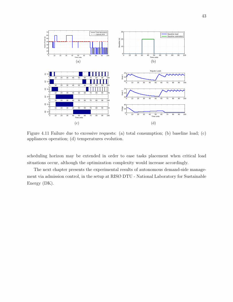
43
0 10 20 30 40 50 60 70 80 90 1000
10
20
30
40
50
60
70
Time units
Inst
ant P
ower
[u]
Total AbsorptionCapacity limit
(a)
0 10 20 30 40 50 60 70 80 90 1000
10
20
30
Bas
elin
e [u
]
Time units
Baseline loadBaseline estimation
(b)
0 10 20 30 40 50 60 70 80 90 1000
0.51
A1
0 10 20 30 40 50 60 70 80 90 1000
0.51
A2
0 10 20 30 40 50 60 70 80 90 1000
0.51
A3
0 10 20 30 40 50 60 70 80 90 1000
0.51
A4
0 10 20 30 40 50 60 70 80 90 1000
0.51
A5
0 10 20 30 40 50 60 70 80 90 1000
0.51
A6
Time units
(c)
0 10 20 30 40 50 60 70 80 90 10020
22
24
Hea
t 1
Regular Loads
0 10 20 30 40 50 60 70 80 90 10020
22
24
Hea
t 2
0 10 20 30 40 50 60 70 80 90 1000
20
40
Frid
ge
Time units
(d)
Figure 4.11 Failure due to excessive requests: (a) total consumption; (b) baseline load; (c)appliances operation; (d) temperatures evolution.
scheduling horizon may be extended in order to ease tasks placement when critical load
situations occur, although the optimization complexity would increase accordingly.
The next chapter presents the experimental results of autonomous demand-side manage-
ment via admission control, in the setup at RISØ DTU - National Laboratory for Sustainable
Energy (DK).

44
CHAPTER 5
EXPERIMENTAL STUDY
5.1 Context
This chapter presents the design, implementation, and the first experimental results of the
presented DSM systems for Smart Buildings in view of optimizing the energy demand in
the Smart Grid. In this study the Admission Control, which is the bottom layer interacting
in real-time with physical equipments, is addressed and the real-time power consumption
management in a residential dwelling is implemented and tested in the FlexHouse at RISØ
DTU. The experimental results provide a proof of concept for the proposed architecture and
demonstrate the applicability of the developed approach in autonomous DSM systems for
Smart Grids.
5.2 The experimental setup: FlexHouse at RISØ DTU
FlexHouse is a test facility organized as an office building that is a part of a SYSLAB research
facility for intelligent, active and distributed systems at RISØ DTU National Laboratory of
Sustainable Energy [RISØ-DTU (2011)]. FlexHouse is equipped as a modern office building,
electrically heated with 10 space heaters and cooled by 4 conditioners. Tap water comes
from a hot water storage tank and the space is illuminated by 24 fluorescent lamps. A
small kitchen consists of a fridge and a coffee machine. Devices in FlexHouse are controlled
remotely. The state of the building and appliances is read from various sensors. FlexHouse
software infrastructure offers interfaces to all devices and easy access to the house’s state as
shown in Fig. 5.1.
Control actions are dispatched by the Home Energy Manager (an implementation of
the proposed DSM architecture), which includes diverse function depending on appliances’
intelligence. Since our aim is to prove a proof of concept for the architecture, the appliance
interface inside this HEM represents only one of the possible implementations. FlexHouse
layout diagram is shown in Fig. 5.2 and the air conditioning is available only in four rooms
out of eight: room 1, room 2, room 3 and the main hall.
Electric heater is installed in all the rooms, while a refrigerator is placed in the main hall
together with the control system, switch panels, and communication devices. The information
system developed for SYSLAB and FlexHouse offers an easy access to actuators and sensors
located in the building or embedded in the appliances. HEM developed in MATLAB can be

45
Figure 5.1 FlexHouse Control Scheme
R1 R2
R8 (Main Hall)
R3 R4
R5
R6R7
Fridge
WH
Figure 5.2 FlexHouse layout & state monitor

46
directly connected to a SYSLAB machine to exchange information with FlexHouse via Java
Remote Method Invocation.
Each device in the FlexHouse is remotely controlled with sensors and actuators based on
EnOcean R© [Anders (2011)] communication standard that offers only one-way communica-
tion and cannot handle acknowledgement exchange. However, the FlexHouse controller is
equipped with a software state mirror that tracks the state of the house by taking into ac-
count all the control signals exchanged between the controller and the devices (see Fig. 5.1).
Thanks to this feature, the HEM can retrieve appliances’ status when needed.
Heaters, lights, and boiler are controlled by EnOcean switches, while the refrigerator is
connected to an EnOcean-based smart plug. The AC, heaters, boiler, and refrigerator have
internal thermostats set to the highest and lowest setpoint respectively, in a way that the
HEM can actively operate the temperature control based on the comfort zones.
Weather information, such as wind direction and speed, solar irradiation, and outside
temperature, is provided by the weather station and the PV panels through dedicated inter-
faces.
Figure 5.3 FlexHouse livingroom
Figure 5.4 FlexHouse and PV installation at RISØ DTU
Since heating and cooling capabilities are available only in five rooms, temperature control
policies have to be designed accurately in order to ensure that heating and cooling systems

47
will be triggered immediately when the temperature is very close to the required room tem-
perature. To this end, we use an hysteresis logic with deadbands in order to manage air
conditioning and heating when they are both available in the same room.
Information on total power consumption is needed when dealing with consumption con-
straints. The air conditioning consumption represents only a limitation, given that it cannot
be estimated and modulated a priori because it depends on inside and outside heat ex-
change conditions (temperature, air flow, humidity, etc.). As the measured air conditioning
consumption is between 250W and 600W, a conservative estimation of constant consump-
tion of 500W is used in operation. The power consumption of heating modules is around
1000W and the refrigerator consumes 60W. Home automation infrastructure has an average
consumption of 300W. Hence, the nominal total consumption of the house is about 11860W,
excluding the baseline load.
5.3 Experimental Results
In this section, we present the experimental results and analyze the performances with respect
to peak shaving and comfort management of such a DSM system.
5.3.1 Power consumption without load management
This experiment aims at demonstrating how the superposition of regular load causes high
peak load. At the beginning, as the temperature of many appliances is outside the comfort
zone, an important number of requests arrive at the same time. Since there is no limitation
on power consumption, the AC will accept all the incoming requests. Temperature evolution
and relative comfort zones in rooms from 1 to 8 (R1, R2,..., R8) are shown in Fig. 5.5(a) and
Fig. 5.5(b). Total power consumption, outside temperature and refrigerator internal tem-
perature are shown in Fig. 5.5(c). Fig. 5.5(a) and Fig. 5.5(b) show that tenants’ comfort is
respected in all rooms. Nevertheless, since air conditioning is not available in all rooms, exter-
nal temperature and solar radiation can cause overheating in some rooms. Fig. 5.5(c) shows
that if there is no control on the accepted requests, at the beginning the peak-consumption
can be as high as 9940W while, after 20 hours of operation, at steady state the highest peak
observed is 7200W.
5.3.2 Peak load shaving via Admission Control
In the experiment reported here, the Admission Control is operated with a constant capacity
limit of 3000W. The DSM system schedules loads using the algorithm presented in Algorithm
1 in order to limit the consumption to the given capacity. We can observe from Fig. 5.6(a)

48
12:00 18:00 00:00 06:00 12:00
18
20
22
R1
14−Sep−2011−with Admission Control
12:00 18:00 00:00 06:00 12:00
20
21
22
R2
12:00 18:00 00:00 06:00 12:0018.5
19
19.5
20
R3
12:00 18:00 00:00 06:00 12:00
26
26.5
27
R4
(a)
12:00 18:00 00:00 06:00 12:0020
22
24
26
R5
14−Sep−2011−with Admission Control
12:00 18:00 00:00 06:00 12:00
20222426
R6
12:00 18:00 00:00 06:00 12:0026.5
27
27.5
28
R7
12:00 18:00 00:00 06:00 12:00
20
22
24
MH
(b)
12:00 18:00 00:00 06:00 12:00
2000
4000
6000
8000
10000
Kw
/h
14−Sep−2011−with Admission Control
Total Cons..Cap. limit
12:00 18:00 00:00 06:00 12:0010
12
14
16
Out
. °C
12:00 18:00 00:00 06:00 12:00
2
3
4
5
Hour
Ref
r. °
C
(c)
12:00 18:00 00:00 06:00 12:00
−8000
−6000
−4000
−2000
0
2000
14−Sep−2011− Consumption deviation
Hour
W
0 20 40 60 80 100 120 1400
500
1000
1500
2000
2500
Measurements
W
Baseline consumption
(d)
Figure 5.5 Case without load management: (a) Temperature in rooms from 1 to 4; (b) tem-perature in rooms from 5 to 8; (c) outside temperature and refrigerator internal temperature;(d) consumption deviation and baseline load.
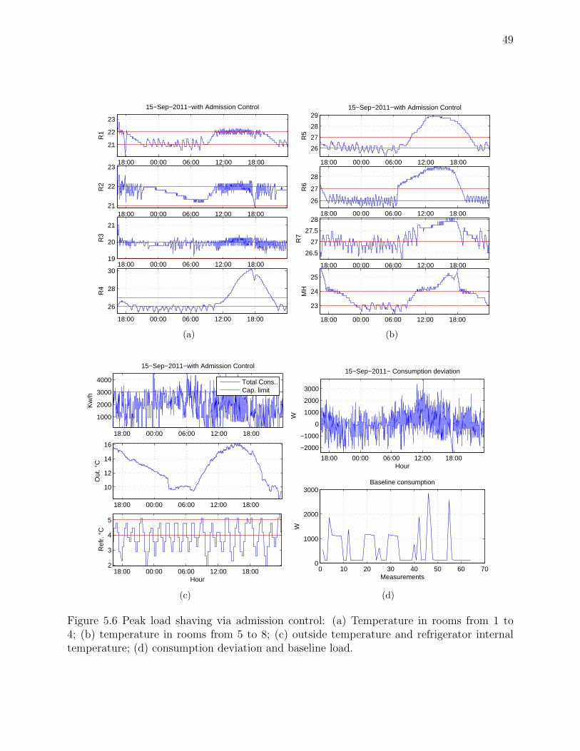
49
18:00 00:00 06:00 12:00 18:00
21
22
23
R1
15−Sep−2011−with Admission Control
18:00 00:00 06:00 12:00 18:0021
22
23
R2
18:00 00:00 06:00 12:00 18:0019
20
21
R3
18:00 00:00 06:00 12:00 18:00
26
28
30
R4
(a)
18:00 00:00 06:00 12:00 18:00
26
27
28
29
R5
15−Sep−2011−with Admission Control
18:00 00:00 06:00 12:00 18:00
26
27
28
R6
18:00 00:00 06:00 12:00 18:00
26.5
27
27.5
28
R7
18:00 00:00 06:00 12:00 18:00
23
24
25
MH
(b)
18:00 00:00 06:00 12:00 18:00
1000
2000
3000
4000
Kw
/h
15−Sep−2011−with Admission Control
Total Cons..Cap. limit
18:00 00:00 06:00 12:00 18:00
10
12
14
16
Out
. °C
18:00 00:00 06:00 12:00 18:002
3
4
5
Hour
Ref
r. °
C
(c)
18:00 00:00 06:00 12:00 18:00
−2000
−1000
0
1000
2000
3000
15−Sep−2011− Consumption deviation
Hour
W
0 10 20 30 40 50 60 700
1000
2000
3000
Measurements
W
Baseline consumption
(d)
Figure 5.6 Peak load shaving via admission control: (a) Temperature in rooms from 1 to4; (b) temperature in rooms from 5 to 8; (c) outside temperature and refrigerator internaltemperature; (d) consumption deviation and baseline load.

50
and Fig. 5.6(b) that the temperature is kept in the comfort zone in all the rooms with AC and
the overheating in the rooms without AC is natural during daytime. The refrigerator internal
temperature is kept in the comfort zone as well, while the peak load is reduced (Fig. 5.6(c))
even if the capacity limit of 3000W is not always respected. In fact the highest peak is
measured to be 4520W and it is caused by different factors, such as the uncertainty on a
appliances’ model (which is based on nominal power consumption) and baseline consumption
variations. For instance the heaters and air conditioning consumption is not constant and
there is no such a way to predict the baseline consumption, given the LF module is not
yet implemented. Such disturbances have a negative impact on the performance of DSM
with respect to the capacity limit compliance, as it is shown by the deviation from nominal
consumption (first chart in Fig. 5.6(d)). The second chart in Fig. 5.6(d) shows the baseline
consumption, which is sampled when all the appliances are turned off and contributes to the
capacity limit violation. Given available historical data and tenants behavioral models, it will
be possible to use them in the Load Forecast module to enhance load shaving performances.
Nevertheless, the DSM system shows its benefits in terms of the reduction of peak con-
sumptions by 61.8% of the maximum nominal consumption (from 11860W to 4520W), by
54.5% in the experimental worst case consumption (at the beginning of the experiment, from
9940W to 4520), and by the 37.2% during steady state operation (from 7200W to 4520W).
5.3.3 Load management via Admission Control and baseline estimation
In order to work around the problem of appliances modeling inaccuracies and lack of LF mod-
ule, in this paragraph we present an ad hoc solution for such specific experimental setup. In
this context, the baseline load is supposed to incorporate the deviation of measured consump-
tion from the expected consumption, which is made up by the summation of nominal power
of running devices. Moreover, the baseline load is supposed to have enough slow dynamics,
such that it may be approximated by the reading value between each pair of samples:
t t+1 t+2 t+3
samplesbaseline
estimated
baseline
Power
Time
Figure 5.7 Baseline estimation

51
In order to compensate the effects of appliances modeling inaccuracies and unavailabil-
ity of accurate measurements of baseline load, at each invocation the Admission Control
subtracts from the available capacity the consumption deviation. This latter value is com-
puted as the difference between the measured total consumption and the sum of each active
appliance nominal power (expected consumption):
Cav(t) = Clim(t)− B(t)
B(t) = Am−∑j
Pjxj
xj∈[0,1] , j∈ N
(5.1)
where Cav is the available capacity, Clim is the capacity limit, B is the estimated baseline
load, Am is the FlexHouse total electric absorption (provided by a central power meter), Pj
is the nominal power consumption of appliance j and xj is its activation status. Fig. 5.8
shows the effectiveness of the proposed solution with respect capacity limit compliance.
5.4 Conclusions
As shown in Section 5.3.3, the effectiveness of peak load shaving is sensitive to appliances
modeling and feedback information, issue that stays open in this research. Indeed, when pass-
ing from simulation to implementation, improve appliances’ models, define tenants’ comfort
metrics, set up adaptive auto-tuning models for the house system are essential achievements.
Those latter futures development is highly interesting given that, concerning temperature
management, appliances influence each others during their operation.

52
09:00 12:00 15:00 18:00
20
21
22
R1
20−Sep−2011−Without Admission Control
09:00 12:00 15:00 18:00
21
21.5
22
R2
09:00 12:00 15:00 18:00
19
19.5
20
R3
09:00 12:00 15:00 18:00
24
25
26
27
R4
(a)
09:00 12:00 15:00 18:00
25
26
27
R5
20−Sep−2011−Without Admission Control
09:00 12:00 15:00 18:00
24
25
26
27
R6
09:00 12:00 15:00 18:00
24
26
28
R7
09:00 12:00 15:00 18:00
22
23
24
MH
(b)
09:00 12:00 15:00 18:00
1000
2000
3000
W
20−Sep−2011−Without Admission Control
Total Cons..Cap. limit
09:00 12:00 15:00 18:00
13
14
15
16
Out
. °C
09:00 12:00 15:00 18:00
4
6
8
10
12
Ref
r. °
C
(c)
09:00 12:00 15:00 18:00
−2000
−1000
0
1000
2000
300020−Sep−2011− Consumption deviation
Hour
W
0 5 10 15 20 25 300
500
1000
1500
2000
2500
Measurements
W
Baseline consumption
(d)
Figure 5.8 Peak load shaving via admission control and baseline estimation: (a) Temperaturein rooms from 1 to 4; (b) temperature in rooms from 5 to 8; (c) outside temperature andrefrigerator internal temperature; (d) consumption deviation and baseline load.

53
CHAPTER 6
CONCLUSIONS AND FUTURE WORK
This research strives at putting forward an original point of view of demand side load man-
agement, proposing a framework for autonomous energy management at customer-side in
the Smart Grid. This framework is suitable for a dynamic environment such as the De-
mand/Response, and can be used at different levels of the Smart Grid. Even though the
implementation proposed in this thesis is in the early stages of development, consistent simu-
lation and experimental results of peak load shaving provided a proof of concept. The chapter
dedicated to the literary review gives an idea of how new the technology of Smart Grids is, and
how fervent the research in this domain is. For instance, the present investigation addresses
and proposes solutions for some aspects of DSM, but does not solve other issues, such as
energy pricing, large-scale optimization, load forecasting, communication technologies, and
Smart Buildings integration within Micro Grids.
For example, an interesting study in [Mardavij Roozbehani (2010),Mardavij Roozbehani
et al. (2011)] presents a new model for electricity real-time retail pricing whereby a feedback
Demand/Response paradigm is proposed and its stability and efficiency are assessed. Con-
cerning the demand-side load management, another interesting point of view is presented
in [Amir-Hamed Mohsenian-Rad et Leon-Garcia (2010)] where a distributed D/R paradigm
is assessed based on a game-theoretic approach. In such distributed architecture, the infor-
mation exchange between customers and utilities tends to explode as the number of users
increases. This is a typical situation in self-organizing systems, where the independence of
each entity has to be traded for the reliability and amount of communication. On the other
hand, centralized control architectures can achieve a higher optimality, at the price of a higher
risk of failure in case of communication collapse between the leader and the clients.
The DSM system proposed here has been conceived with a layered architecture based
on the decentralized/hierarchical control paradigm, where each layer operates independently
and at maximum of its potential. This allows to reduce drammatically the communication
between layers, which occurs in the case of insufficient information or infeasible solutions,
information exchange between users and information exchange between users and utilities.
Smart Buildings integration with Micro Grids and renewable energy sources is among
the most interesting applications of such a DSM system, a topic that is assessed in [Xiao-
hong Guan et Jia (2010)]. In this latter study a mixed-integer optimization approach is
used to coordinate all the loads and energy sources in the Micro Grid. An issue rising up

54
from such a complex model is the computational feasibility with respect to time constraints.
This latter argument addresses future research on optimization problems and sub-optimal
strategies applied to real-time energy market and load scheduling.
Even if the demand-side management is only one feature, it is an enabling technology for
many components of the Smart Grid. Efficient DSM will enable a high penetration of renew-
able energy sources such as solar and wind power, and the integration of Smart Buildings
with local generation in the micro grids. It will give the means for effective electricity dy-
namic pricing and liberalization of energy markets, where the customers will be encouraged
to consume less and be more efficient so as to minimize their energy expenses. Such prac-
tices have immediate benefits for the environment, thus allowing for its protection, making
it economically viable.
From these latter considerations, one can think about another realm of possible develop-
ments in terms of energy trading. In fact, as energy demand is constantly increasing, various
energy trading companies have been recently established. Such business is very attractive for
utilities, traders, and customers, and is based on customer aggregation. There exist compa-
nies that offer load shedding services to the grid by contracting consumption decrease with
their customers. In such a context, customers are asked by the aggregator to modify their
consumption for a given time period, in exchange of an economical incentive. In this way,
the aggregator can offer ancillary services to utilities by offering load shadding, service that
has a consistent economic value depending on the moment it is offered. At the current state
of the art, such kind of DSM is operated via manual customer notification. However, in the
near future, this system may be enabled to aperate automatically. As a natural evolution of
this latter practice, one can think about commercial customers, for instance whose shedding
capacity may be considerable in the case of shopping malls. With this vision, it is not diffi-
cult to imagine that typical practices of stock markets may be applied to the energy market.
Evidently, the aformentioned topic raises up ethical and social issues, whose investigation
will hopefully be exhaustively carried out.
In conclusion, I hope this research constitutes a starting point for future developments in
the fields of engineering, mathematics, social sciences, and economics, in the light of putting
Science at the service of Humanity and environment preservation.

55
REFERENCES
A. CAPASSO ET AL. (1994). A bottom-up approach to residential load modeling. IEEE
Transactions on Power Systems, 9, pp. 957–964.
AMIR-HAMED MOHSENIAN-RAD, VINCENT W S WONG, J. J. R. S. et LEON-
GARCIA, A. (2010). Autonomous demand-side management based on game-theoretic en-
ergy consumption scheduling for future smart grid. IEEE Transactions on Smart Grid, 1,
320–331.
ANDERS, A. (2011). Enocean technology energy harvesting wireless. Rapport technique,
EnOcean GmbH.
BELLIFEMINE, F.L. ET AL. (2009). Smart grid: Energia & ict. Notiziario tecnico Telecom
Italia, 3, pp. 15–32.
BUTTAZZO, G. (2005). Hard Real Time Computing Systems - Predictable Scheduling Al-
gorithms and Applications. Springer, New York, seconde edition.
CHIA-HUNG LIEN ET AL. (2008). Power monitoring and control for electric home ap-
pliances based on power line communication. IEEE International Instrumentation and
Measurement Technology Conference, Victoria, Vancouver Island (CA).
C.S. CHEN ET AL. (1997). Application of load survey systems to proper tariff design.
IEEE Transactions on Power Systems, 12, pp. 1746–1751.
DRAKE, J., NAJEWICZ, D. et WATTS, W. (2010). Energy efficiency comparisons of wire-
less communication technology options for smart grid enabled devices. Rapport technique,
General Electric Company, GE Appliances & Lighting.
DRURY CRAWLERY, S. P. et TORCELLINI, P. (2009). Getting to net zero. National
Research Laboratory, Journal Article NREL/JA-550-46382.
E. MUSALL ET AL. (2010). Net zero energy solar buildings: An overview and analysis on
worldwide building projects. Rapport technique, Department of Architecture, University of
Wuppertal, Wuppertal (Germany).
EUROPEAN COMMISSION, DG ENERGY, A. (2011). Eu energy portal.

56
F.KELLY, A. et D.TAN (1998). Rate control for communication networks: shadow prices,
proportional fairness, and stability. Journal of the Operational Research Society, 49, 237–
252.
FLYNN, B. (2008). Key smart grid applications. The Protection & Control Journal (G.E).
GUAN, X., XU, Z. et JIA, Q.-S. (2010). Energy-efficient buildings facilitated by microgrid.
IEEE Trans. on Smart Grid, 1, 243–252.
HOLMAN, J. (1997). Heat Transfer. McGraw-Hill, NY, 8th edition.
IEEE-P2030 (2011). 2030 Smart Grid Interoperability Series of Standards.
IFC CONSULTING (Feb. 2009). The economic cost of the blackout: An issue paper on the
northeastern blackout, august 14, 2003. Rapport technique, IFC Consulting.
IQBAL, M. (2004). A feasibility study of a zero energy home in newfoundland. Renewable
Energy Review, Elsevier, 29, pp. 277–289.
J.NICHOLS ET AL. (2002). Generating remote control interfaces for complex appliances.
Proceedings of the 15th annual ACM symposium on User interface software and technology,
Paris, 4, pp. 161–170.
JOHN F. NASH, J. (1951). Non-cooperative games. Annals of Mathematics, 52, 286–295.
KADAM, S. (Spring 2001). Zero net energy buildings: Are they economically feasible?
Rapport technique, MIT - Massachusetts Institute of Technology.
KENNETH P. WACKS ET AL. (1991). Utility load management using home automation.
IEEE Transactions on Consumer electronics, 37, pp. 168–174.
KLEISSI, J. et AGARWAL, Y. (2010). Cyber-physical energy systems: Focus on smart
buildings. Preceedings of Annual ACM/IEEE Design Automation Conference, pp. 749–754.
KLEMPER, P. et MEYER, M. (1989). Supply function equilibria in oligopoly uncertainty.
Econometrica, 57, 1243–1277.
LI, J. et SUN, R. (2010). Information appliance controller was developed based on power line
carrier communication. 2010 International Conference on Networking and Digital Society.
Wenzhou, China, 571–574.
LIJUN CHAN, NA LI, S. H. L. et DOYLE, J. (2010). Two market models for demand re-
sponse in power networks. IEEE International Conference on Smart Grid Communications.

57
LUKAS G. SWAN ET AL. (2009). Modeling of end-use energy consumption in the residen-
tial sector: A review of modeling techniques. Renewable and Sustainable Energy Reviews,
Elsevier, 13, pp. 1819–1835.
MARDAVIJ ROOZBEHANI, MUNTHER DAHLEH, S. M. (2010). On the stability of
wholesale electricity marjets under real-time pricing. 49th IEEE Conference on Decision
and Control. Atalanta, USA.
MARDAVIJ ROOZBEHANI ET AL. (2011). Analysis of competitive electricity markets
under a new model of real-time retail pricing with ex-post adjustment. 8th International
Conference on the European Energy Market.
MCDONALD, J. (2010). The smart grid. Paris energy summit.
N. KUSHIRO ET AL. (2003). Integrated residential gateway controller for home energy
management system. IEEE Transaction on Consumer Electronics, 9, pp. 629–636.
NEENAN, B. (2008). Societal benefits of smart metering investments. The Electricity
Journal, 21, pp. 32–45.
RAAIJ, W. F. V. et VERHALLEN, T. M. (1983). A behavioral model of residential energy
use. Journal of Economic Psychology, 3, pp. 39–63.
RISØ-DTU (2011). National laboratory for sustainable energy, technical university of den-
mark. http://www.risoe.dtu.dk.
S. BRUNO ET AL. (2009). Load control through smart-metering on distribution networks.
IEEE Bucharest PowerTech.
S. KARNOUSKOS ET AL. (2007). An advanced metering infrastructure for future energy
network. New technologies, Mobility and Security, Springer, pp. 597–606.
SCHNEIDER ELECTRIC CORP. (2010). Perspectives and priorities - schneider electric
on smart grid research. Canada Smart Grid Research Network Workshop British Columbia
Insitute of Technology.
SIMON, A. et BELLES, R. (2009). Estimated state level energy flows in 2008. Rapport
technique, Lawrence Livermore National Laboratory.
STANKOVIC, J. A. et RAMAMRITHAN, K. (1989). The spring kernel: A new paradigm
for real time operating systems. Rapport technique, University of Massachussets, Dept. of
Computer and Information Science.

58
THE MATHWORKS INC. (2011). Optimization toolbox documentation - binprog.
UTILIPOINT (2010). Pricing D/R Reports.
V. POTHAMSETTY AND S. MALIK (February 2009). Smart grid: Leveraging intelligent
communications to transform the power infrastructure. Rapport technique, CISCO Systems
(white paper).
XIAOHONG GUAN, Z. X. et JIA, Q.-S. (2010). Energy-efficient buildings facilitated by
microgrid. IEEE Transactions on Smart Grid, 1, 243–252.
YU-JU LIN ET AL. (2002). A power line communication network infrastructure for the
smart home. IEEE Wireless Communications review, 9, pp. 104–111.
ZHONG, F. (2010). Distributed demand-response and user adaptation in smart grids.
Rapport technique, Toshiba Research Europe Laboratory.

59
ANNEX A
MATLAB CODE OF ADMISSION CONTROL BLOCK
1 %##########################################################################2 % Copyright: Giuseppe Tommaso Costanzo3 % Partners: Ecole Polytechnique de Montreal, Politecnico di Milano4 % Last rev: August 10, 20115 % Contact info: [email protected] % [email protected] %8 % The usage of any part of this code for commercial pouposes should be9 % authorized by the author. Any part of this code can be used for academic
10 % purposes upon citation.11 %##########################################################################12 % request(1)= appliance id {1..N}13 % request(2)= appliance status {1,2,3,4,5,6}, (1=off, 2=ready, 3=run,14 % 4=idle, 5=complete, 6=fault)15 % request(3)= preemption {0,1}16 % request(4)= required energy (1..E)17 % request(5)= heuristic value (0,1)18 % request(6)= power load {0,P}19 % request(7)= execution flag {0,1}20 % request(8)= arrival time {t}21 % request(9)= deadline {t,t+m}22
23 function [accepted,rejected,rej_rate]=admissioncontrol(C,request_m)24
25 % NB: when you want to deactivate the AC you need to change three26 % things in the program: treshold, commented parts in the last loop of AC,27 % and rise up the capacity in the initialization script sim_init.m28
29 request_matrix=sort_heuristic(request_m);30 rjr=0;31 m=size(request_matrix,1);32 %treshold=0; environment=0;% to use when we don’t want the AC active...33 treshold=0.3; environment=1;34 tot=0;35
36 %##########################################################################37 % here we create the support vector for the acctivations38 act=zeros(1,m);39
40 %##########################################################################41 % here we accept those requests that belongs to tasks that are42 % non-preemptive and were operating at the previous time frame.43 for k=1:m44 if (request_matrix(k,1)~=0 && request_matrix(k,2)==3 && request_matrix45 (k,3)==0 && request_matrix(k,4)>0.1)46 act(request_matrix(k,1))=1;

60
47 tot=tot+request_matrix(k,6);48 request_matrix(k,:)=0;49 end50 end51
52 %##########################################################################53 % here we accept those requests that respect the schedulability condition54 % and have been running at the previous time frame or have maximum55 % heuristic value56 for k=1:m57 if (request_matrix(k,1)~=0 && tot+request_matrix(k,6)<=C &&58 treshold<request_matrix(k,5) && request_matrix(k,2)==3 &&59 request_matrix(k,4)>0.1)60 act(request_matrix(k,1))=1; % activation flag61 tot=tot+request_matrix(k,6);62 request_matrix(k,:)=0;63 end64 end65
66 %##########################################################################67 % here we fill the remaining capacity with the remaining requests68
69 if environment70 for k=1:m71 if (request_matrix(k,1)~=0 && tot+request_matrix(k,6)<=C &&72 0.6<request_matrix(k,5) && request_matrix(k,4)>0.1)73 act(request_matrix(k,1))=1; % activation flag74 tot=tot+request_matrix(k,6);75 request_matrix(k,:)=0;76 end77 end78 else79 for k=1:m80 if ((request_matrix(k,1)==4||request_matrix(k,1)==5||81 request_matrix(k,1)==6) && tot+request_matrix(k,6)<=C &&82 0<request_matrix(k,5) && request_matrix(k,4)>0.1)83 act(request_matrix(k,1))=1; % activation flag84 tot=tot+request_matrix(k,6);85 request_matrix(k,:)=0;86 else87 if (request_matrix(k,1)~=0 && tot+request_matrix(k,6)<=C &&88 0.6<request_matrix(k,5) && request_matrix(k,4)>0.1)89 act(request_matrix(k,1))=1; % activation flag90 tot=tot+request_matrix(k,6);91 request_matrix(k,:)=0;92 end93 end94 end95 end96 accepted=act;97 rej=not(act);98 for i=1:m99 if request_m(i,4)<1 %if the required energy is small, the task should
100 %not belong to the rejected tasks

61
101 rej(i)=0;102 end103 end104 rej_rate=sum(rej);105 rej(1:3)=0;106 rejected=rej;107 end108
109 % ########## FUNCTION SORT HEURISTIC ##########110 function list=sort_heuristic(requests)111 b=size(requests,1);112 temp=[(1:b)’ zeros(b,1)];113 req=zeros(size(requests));114 for j=1:b115 temp(j,2)=requests(j,5);116 end117 [B,I]=sort(temp,1,’descend’);118 temp=[I(:,2) B(:,2)];119 for j=1:b120 req(j,:)=requests(temp(j,1),:);121 end122 list=req;123 end

62
ANNEX B
MATLAB CODE OF LOAD BALANCER BLOCK
1 %##########################################################################2 % Copyright: Giuseppe Tommaso Costanzo3 % Partners: Ecole Polytechnique de Montreal, Politecnico di Milano4 % Last rev: Sept 6, 2011 - Simulink version5 % Contact info: [email protected] % [email protected] %8 % The usage of any part of this code for commercial pouposes should be9 % authorized by the author. Any part of this code can be used for academic
10 % purposes upon citation.11 %##########################################################################12 function output_sched=loadbalancer(rejected,request_matrix,schedule,C,K)13 m=size(schedule,1);14 coder.extrinsic(’loadbalancerSIMULINK’,’datestr’,’now’,’displayrequests’)15 displayrequests(request_matrix)16 rejected17 tobalance=request_matrix(rejected,:)18 a=datestr(now)19 SCHED=schedule;20 SCHED=loadbalancerSIMULINK(tobalance,schedule,C’,K’);21 output_sched=[(1:m)’ SCHED(:,2:end)]22 end

63
ANNEX C
MATLAB CODE OF LOAD BALANCER BALGORITHM
1 %##########################################################################2 % Copyright: Giuseppe Tommaso Costanzo3 % Partners: Ecole Polytechnique de Montreal, Politecnico di Milano4 % Last rev: October 10, 20115 % Contact info: [email protected] % [email protected] %8 % The usage of any part of this code for commercial pouposes should be9 % authorized by the author. Any part of this code can be used for academic
10 % purposes upon citation.11 %##########################################################################12 % request(1)= appliance id {1..N}13 % request(2)= appliance status {1,2,3,4,5,6}, (1=off, 2=ready, 3=run,14 % 4=idle, 5=complete, 6=fault)15 % request(3)= preemption {0,1}16 % request(4)= required energy (1..E)17 % request(5)= heuristic value (0,1)18 % request(6)= power load {0,P}19 % request(7)= execution flag {0,1}20 % request(8)= arrival time {t}21 % request(9)= deadline {t,t+m}22
23 function output_sched=loadbalancerSIMULINK(request_matrix,schedule,C,K)24
25 %request_matrix26 m=size(request_matrix,1);27 n=size(schedule,2)-1; % remember that the first column of the schedule is28 % not a time frame, but contains the ids...29 display(sprintf(’Entering the Load Balancer... n=%u , m=%u’,n,m));30
31 %fictitious arrival times definition32 display(’LB: Arrival times’)33 a=request_matrix(:,8)’34
35 % deadlines definition36 display(’LB: Deadlines’)37 d=floor(request_matrix(:,9)’)/1038
39 % tasks energy requests40 display(’LB: Energy requests’)41 e=request_matrix(:,4)’42
43 % tasks power requests44 display(’LB: Power requests’)45 p=request_matrix(:,6)’46

64
47 % available capacity profile48 display(strcat(’Capacity profile:’,num2str(C)));49 OPTIONS=optimset(’Algorithm’,’sqp’,’NodeSearchStrategy’,’df’,’MaxTime’,60,50 ’Display’,’iter’);51 utl=100*sum(e)/sum(C);52 display(strcat(’Utilization factor : ’,num2str(utl),’ %’))53 if (utl>100)||(max(p)>max(C))54 display(’The problem is unfeasible because of the capacity’)55 output_sched=[];56 else57 %######### Activation vectors58 act={};59 shift={};60 shift2={};61 tau=[];62 A0=[];63 A1=[];64 A2=[];65 b=[];66 b0=[];67 K1=[];68 Aeq=[];69
70 for j=1:m %appliances71 act{j}=zeros(1,n);72 act{j}(1,a(j):d(j))=1; % activation vector for task j73 Aeq=blkdiag(Aeq,not(act{j})); % constraints on the activation.74 %this set forces to zero those xij outside the admissibility range75 tau(j)=ceil(e(j)/p(j)); %ok76 h(j)=n-tau(j); %ok77 % costruzione matrice di shift78 for y=1:h(j)+179 base=zeros(1,n);base(y:y+tau(j)-1)=1;80 shift{j,y}=diag(base); %ok81 shift2{j,y}=zeros(n,n);shift2{j,y}(:,y)=-base; %ok82 end83 A0=[A0 p(j)*eye(n)];84 b0=[b0;-e(j)];85 K1=[K1 K*p(j)]; %objective function: power*cost/unit86 end87
88 A0=[A0 zeros(size(A0))];89
90 % matrix shift contains occurrences of the state variables x91 for j=1:size(shift,1)92 for y=1:size(shift,2)93 if size(shift{j,y},1)==094 shift{j,y}=zeros(n,n);95 end96 end97 end % putting zeros where there is no shift matrix98 for y=1:size(shift,2)99 A1=[A1;blkdiag(shift{:,y})];
100 end

65
101 % matrix shift2 contains occurrences of activation variables d102 for j=1:size(shift2,1)103 for y=1:size(shift2,2)104 if size(shift2{j,y},1)==0105 shift2{j,y}=zeros(n,n);106 end107 end108 end % putting zeros where there is no shift2 matrix109 for y=1:size(shift2,2)110 A2=[A2;blkdiag(shift2{:,y})];111 end112
113 A=-[A1 A2];114 A=[A0;A];115 b=zeros(size(shift,2)*n*m,1);116 b=[C’;b];117 beq=[zeros(1,m)’;ones(1,m)’];118 K1=[K1 zeros(1,m*n)];119
120 for j=1:m121 vect=ones(1,n);122 vect(end-tau(j)+2:end)=0;123 Aeq=blkdiag(Aeq,vect);124 end125
126 problem1.f=K1;127 problem1.Aineq=A;128 problem1.bineq=b;129 problem1.Aeq=Aeq;130 problem1.beq=beq;131 problem1.solver=’bintprog’;132 problem1.options=OPTIONS;133
134 tic135 [x,fval,EXITFLAG,OUTPUT]=bintprog(problem1);136 toc137
138 if isempty(find(x,1))139 output_sched=schedule;140 else141 SCHED=[];142 y=0;143 for j=1:m144 for i=1:n145 y=y+1;146 SCHED(j,i)=schedule(j,i+1)+(x(y)*p(j));147 end148 end149 SCHED2=schedule;150 if not(isempty(SCHED))151 % the following line updates the schedule with the tasks that152 % have been placed by the load balancer153 SCHED2(request_matrix(:,1),2:end)=SCHED;154 else

66
155 SCHED2=schedule;156 end157 output_sched=SCHED2;158 end159 end160 end

67
ANNEX D
MATLAB CODE OF REQUEST GENERATOR
1 %##########################################################################2 % Copyright: Giuseppe Tommaso Costanzo3 % Partners: Ecole Polytechnique de Montreal, Politecnico di Milano4 % Last rev: August 10, 20115 % Contact info: [email protected] % [email protected] %8 % The usage of any part of this code for commercial pouposes should be9 % authorized by the author. Any part of this code can be used for academic
10 % purposes upon citation.11 %##########################################################################12 % request(1)= appliance id {1..N}13 % request(2)= appliance status {1,2,3,4,5,6}, (1=off, 2=ready, 3=run,14 % 4=idle, 5=complete, 6=fault)15 % request(3)= preemption {0,1}16 % request(4)= required energy (1..E)17 % request(5)= heuristic value (0,1)18 % request(6)= power load {0,P}19 % request(7)= execution flag {0,1}20 % request(8)= arrival time {t}21 % request(9)= deadline {t,t+m}22 function requests = requestgen(signals, schedule)23 m=6;24 schedule;25 request_matrix=zeros(6,9);26 h=0;27 for k=1:m28 for i=1:929 h=h+1;30 request_matrix(k,i)=signals(h);31 end32 end33 a=diag(sum(schedule(:,2:end),2)==0);34 requests=[(1:m)’ a*request_matrix(:,2:end)];35 end

68
ANNEX E
MATLAB CODE OF SCHEDULE MANAGER
1 %##########################################################################2 % Copyright: Giuseppe Tommaso Costanzo3 % Partners: Ecole Polytechnique de Montreal, Politecnico di Milano4 % Last rev: October 20, 20115 % Contact info: [email protected] % [email protected] %8 % The usage of any part of this code for commercial pouposes should be9 % authorized by the author. Any part of this code can be used for academic
10 % purposes upon citation.11 %##########################################################################12 function [C_used,sched,count1]=schedulemanager(control,new_schedule,schedule,time,count)13 m=size(schedule,1);14 if isequal(control,new_schedule)15 sched_t=schedule;16 else17 sched_t=new_schedule;18 end19 count1=((1+floor(time/10))*10);20 if (count==count1)21 sched=sched_t;22 else23 sched=[(1:m)’ sched_t(:,3:end) zeros(m,1)];24 end25 C_used=sum(sched(:,2));26 end

69
ANNEX F
MATLAB CODE OF DISPATCHER
1 %##########################################################################2 % Copyright: Giuseppe Tommaso Costanzo3 % Partners: Ecole Polytechnique de Montreal, Politecnico di Milano4 % Last rev: October 6, 20115 % Contact info: [email protected] % [email protected] %8 % The usage of any part of this code for commercial pouposes should be9 % authorized by the author. Any part of this code can be used for academic
10 % purposes upon citation.11 %##########################################################################12 function [act,op]=dispatcher(active,schedule)13 m=size(schedule,1);14 open=zeros(1,m);15 for k=1:m16 if schedule(k,2)~=017 open(k)=1;18 else19 open(k)=0;20 end21 end22 op=open;23 act=active+open;24 end

70
ANNEX G
MODEL PARAMETERS INITIALIZATION
1 % parameters initialization of the DSM simulator2 warning off3 clc4 %simulation time parameters5 sim_time=100;6 clock_period=0.01;7 sched_timeframe=10; %how many second there are in one schedule time frame8 n=10; %number of timeframes of the schedule - places to update: Cap_manager19 counter_reset=sched_timeframe/clock_period;
10 %appliances11 m=6; % number of appliances12 act_signals_init=zeros(1,m);13
14 dryer_deadline=40;15 washm_deadline=40;16 dishw_deadline=70;17
18 C=60*ones(1,sim_time/sched_timeframe);19 K=3000*ones(1,sim_time/sched_timeframe);20