Demand, Load and Spill AnalysisDr. Peter Belobaba

Network, Fleet and Schedule

Strategic Planning

Module 13 :   12  March 2014

Istanbul Technical University

Air Transportation Management 

M.Sc. Program 

2

Lecture Outline

Terms and Definitions Demand, Load and Spill Airline Demand Variability

Spill Analysis: Boeing Spill Model Estimating Spill Given Observed Load Factors Use of Spill Tables Impacts of Different Size Aircraft

Applications to Cabin Configuration

Spill and Recapture Across Multiple Flights

Impacts of RM on Spill

3

Terms and Definitions

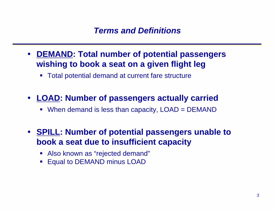
DEMAND: Total number of potential passengers wishing to book a seat on a given flight leg Total potential demand at current fare structure

LOAD: Number of passengers actually carried When demand is less than capacity, LOAD = DEMAND

SPILL: Number of potential passengers unable to book a seat due to insufficient capacity Also known as “rejected demand” Equal to DEMAND minus LOAD

4

“Spill” vs. “Denied Boardings”

SPILL occurs when potential demand for a flight leg is greater than the physical capacity of the aircraft Spill can occur whether or not the airline is using overbooking

methods For spill analysis, typically assume no overbooking or “perfect”

overbooking in which no-shows are predicted correctly Spill occurs during the pre-departure booking process

DENIED BOARDINGS occur on overbooked flights when more passengers than capacity show up Denied boardings occur because the airline overbooked too

aggressively, not because the aircraft was too small DBs occur at the gate just before departure

5

Airline Demand Variability

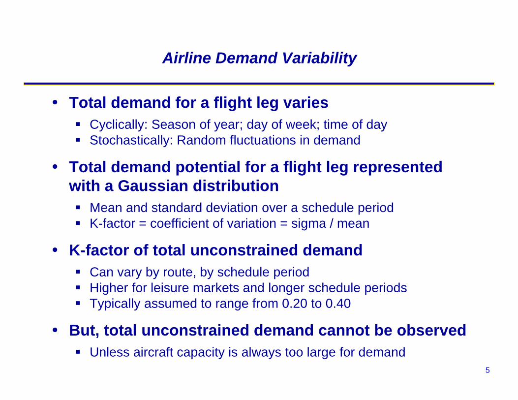
Total demand for a flight leg varies Cyclically: Season of year; day of week; time of day Stochastically: Random fluctuations in demand

Total demand potential for a flight leg represented with a Gaussian distribution Mean and standard deviation over a schedule period K-factor = coefficient of variation = sigma / mean

K-factor of total unconstrained demand Can vary by route, by schedule period Higher for leisure markets and longer schedule periods Typically assumed to range from 0.20 to 0.40

But, total unconstrained demand cannot be observed Unless aircraft capacity is always too large for demand

6

Example: Individual Flight Departures

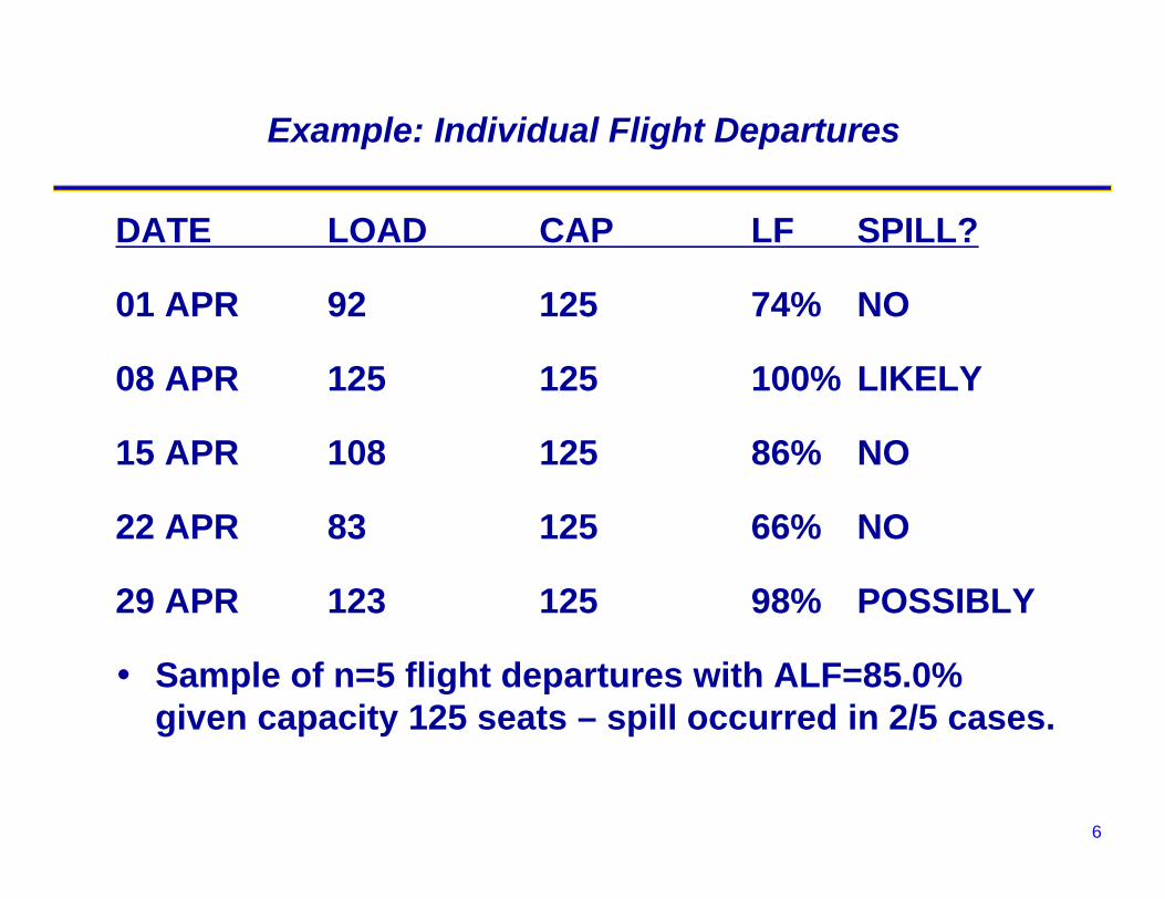
DATE LOAD CAP LF SPILL?

01 APR 92 125 74% NO

08 APR 125 125 100% LIKELY

15 APR 108 125 86% NO

22 APR 83 125 66% NO

29 APR 123 125 98% POSSIBLY

Sample of n=5 flight departures with ALF=85.0% given capacity 125 seats – spill occurred in 2/5 cases.

7

Frequency Histogram of Flight Loads

Source: Boeing (1978)

8

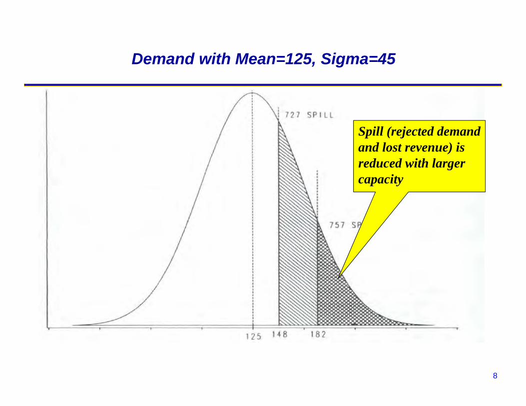
Demand with Mean=125, Sigma=45

Spill (rejected demand and lost revenue) is reduced with larger capacity

9

Spill Analysis: Boeing Spill Model

Objective: Estimate actual “unconstrained” demand for a sample of flights where spill has occurred.

Observations: Sample of flight leg loads (constrained) over a representative time period: Perhaps adjusted for future seasonality and/or traffic growth

Assumptions: Unconstrained demand for a series of flight departures can be

represented by a Gaussian distribution We use observed Average Load Factor and an ASSUMED

k-factor to estimate unconstrained demand

Boeing Spill Tables can be used to minimize calculations

10

Example: Sample of Flight Departures

Mean load = 106.2 passengers (85.0% LF) with observed standard deviation= 18.6 But, observed sigma constrained by capacity Both mean and sigma are therefore smaller than actual demand

Assume K=0.35 for unconstrained demand Based on “market knowledge” and expected demand variability

during schedule period under consideration

Spill Table (K=0.35) shows relationships between AVERAGE LOAD FACTOR = Mean Load/Capacity DEMAND FACTOR = Mean Demand/Capacity SPILL FACTOR = Mean Spill/Capacity

“Spill Rate” = Mean Spill / Mean Demand Historical target for spill rate is 5-10% or less

11

Spill Table for K=0.35

DF and SF given LOAD FACTORLF DF SF LF DF SF

• Assuming underlying demand has K=0.35

• Then, 0.850 observed average load factor translates to 0.972 demand factor and 0.122 spill factor

• Load factor = demand factor – spill factor

Source: Boeing

12

Spill Table Calculations

Given observed LF and assumed K=0.35 DF = 0.972 from Table, and SF = 0.122 [Note that DF = LF + SF, always!]

We can now calculate the following estimates: Mean total demand = DF * Capacity = 0.972*125= 121.5

Std deviation of Demand = 0.35 * 121.5 = 42.5

Mean spill per departure = SF * Capacity = 0.122*125 = 15.3[NOTE also: Mean Spill = Mean Demand – Mean Load]

Spill Rate = Mean Spill/Mean Demand = 15.3 / 121.5 = 12.6%

13

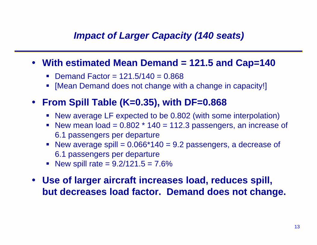
Impact of Larger Capacity (140 seats)

With estimated Mean Demand = 121.5 and Cap=140 Demand Factor = 121.5/140 = 0.868 [Mean Demand does not change with a change in capacity!]

From Spill Table (K=0.35), with DF=0.868 New average LF expected to be 0.802 (with some interpolation) New mean load = 0.802 * 140 = 112.3 passengers, an increase of

6.1 passengers per departure New average spill = 0.066*140 = 9.2 passengers, a decrease of

6.1 passengers per departure New spill rate = 9.2/121.5 = 7.6%

Use of larger aircraft increases load, reduces spill, but decreases load factor. Demand does not change.

14

Spill Table for K=0.35

LF and SF given DEMAND FACTORDF LF SF DF LF SF • Assuming underlying

demand has K=0.35

• Then, 0.870 estimated demand factor translates to 0.803 average load factor and 0.067 spill factor

• Demand factor = load factor + spill factor

Source: Boeing

15

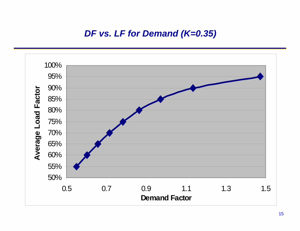
DF vs. LF for Demand (K=0.35)

50%55%60%65%70%75%80%85%90%95%

100%

0.5 0.7 0.9 1.1 1.3 1.5Demand Factor

Aver

age

Load

Fac

tor

16

Alternative Aircraft Capacities

Should the airline operate a 140-seat aircraft to serve this demand distribution?

Increasing capacity by 15 seats expected to increase average load per departure by 6.1 passengers Increase in revenue per flight = 6.1 passengers * average fare

But, changing this fleet assignment to a larger aircraft will increase operating costs as well Increase in operating costs = difference in cost/block-hour *

number of block-hours for flight leg in question

17

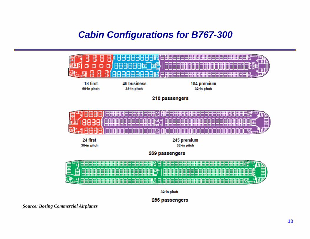
Applications to Cabin Configuration

Additional seats in Premium Class reduce premium spill and increase revenues; but reduction in Economy seats increases economy spill and reduces economy revenue

Spill model can be used to estimate the trade-off in premium revenue gain vs. economy revenue loss

Premium Capacity Economy Capacity

18

Cabin Configurations for B767-300

Source: Boeing Commercial Airplanes

19

Spill and Recapture Across Multiple Flights

Source: Abramovich (2013)

20

Reduced Flight 1 Capacity

Source: Abramovich (2013)

21

Increase Flight 1 Capacity

Source: Abramovich (2013)

22

Revenue management system generates booking limits for each class to maximize revenue

Protect seats for high fare passengers, reject low-fare bookings when demand factor is high

RM Systems Reject Demand

CABIN CAPACITY = 135AVAILABLE SEATS = 135

BOOKING AVERAGE SEATS FORECAST DEMAND JOINT BOOKINGCLASS FARE BOOKED MEAN SIGMA PROTECT LIMIT

Y 670$ 0 12 7 6 135M 550$ 0 17 8 23 129B 420$ 0 10 6 37 112V 310$ 0 22 9 62 98Q 220$ 0 27 10 95 73L 140$ 0 47 14 40

SUM 0 135Source: Abramovich (2013)

23

0

20

40

60

80

100

120

70 90 110 130 150 170 190 210 230 250

Total M

argina

l Reven

ue Per Seat

Capacity

0

10

20

30

40

50

60

70

80

70 80 90 100 110 120 130 140 150 160 170 180

Revenu

e (Tho

usan

ds)

Capacity

6

5

4

3

2

1

Impacts of RM on Marginal Revenue

Standard Leg RM

Fare Class Mix Marginal Revenue

Marginal revenue per additional seat decreases with increasing capacity.

Most additional bookings are in lower classes.

Source: Abramovich (2013)