Demand for Battery-electric & Plug-in Hybrid Vehicles:Policy Lessons for an Emerging Market

Tamara L. Sheldon∗1, J.R. DeShazo†2, and Richard T. Carson‡3

1Department of Economics, University of South Carolina2Luskin School of Public Affairs, University of California, Los Angeles

3Department of Economics, University of California, San Diego

[Latest update: September 22, 2015]

Abstract Understanding demand in the new plug-in hybrid electric vehicle (PHEV) mar-

ket is critical to designing more effective adoption policies. We use stated preference data

from an innovative choice experiment to estimate demand for PHEVs relative to battery elec-

tric vehicles (BEVs) and to explore heterogeneity in demand for these vehicle technologies.

We find that the gap between willingness to pay for PHEVs and their price premium over

conventional vehicles is on the order of current subsidies, while that of BEVs is an order of

magnitude larger. We also find evidence that consumers with access to HOV lanes are more

likely to purchase PHEVs and that the characteristics of the home charging environment are

more important for BEV purchase decisions. Finally, we use a latent class model to show

that PHEVs draw an entirely new consumer segment into the electric vehicle market that

would not consider purchasing a BEV.

∗Tamara.Sheldon@moore.sc.edu†deshazo@ucla.edu‡rcarson@ucsd.edu

1

1 Introduction

Policymakers have sought to spur demand for plug-in electric vehicles (PEVs) through a

variety of policy incentives. The economic rationale for the design of these policy incentives

has been based on the presence and size of environmental and knowledge-spillover externali-

ties. The desired effect of policies targeting these externalities is to adjust consumers’ ex post

demand for these vehicles in ways that enhance overall social welfare. However, understand-

ing of consumer demand for these vehicles and associated interactions with policy incentives

is incomplete because automakers have recently differentiated their plug-in electric vehicle

product mix.

Automakers have added plug-in hybrid electric vehicles (PHEVs), which may be fueled

by either electricity or gasoline, to the early mix of battery electric vehicles (BEVs), which

are fueled only by electricity. By adding PHEVs, automakers sought to eliminate consumers’

“range anxiety” associated with the limited travel range of smaller-battery BEVs. PHEVs also

represented a vehicle design innovation that enabled many automakers to adapt pre-existing

vehicle designs to plug-in electric refueling, thus eliminating their need to design entirely new

models. For instance, there are now PEV versions of the Ford Fusion and Honda Accord,

as well as the Mitsubishi Outlander and the Porsche Panamera. The attractiveness of the

PHEVs relative to BEVs to automakers has been revealed by the decision to introduce a

substantial number of PHEVs to the market (see Table 1) with plans for many more in the

relatively near future as rumored in the trade press (e.g., the Audi A3 e-tron and the Hyundai

Sonata Plug-in). Consumers have thus far exhibited a preference for PHEVs relative to BEVs

by purchasing relatively more of them, as shown Figure 1.

Within the literature, researchers have undertaken innovative studies of consumer de-

mand for BEVs (Bunch et al., 1993; Brownstone, Bunch, and Train, 2000; Hidrue et al.,

2011), however, research on PHEV demand remains limited. Most existing research studies

were implemented before PHEVs were commercially available and they focused on design

priorities for vehicle attributes (Kurani, Heffner, and Turrentine, 2008; Axsen and Kurani,

2

2009) as well as qualitative market trial studies (Caperello and Kurani, 2012; Graham-Rowe

et al., 2012).

Table 1: PEV Model Introductions

2012-2013 2014-2015

Model Make PEV Type Model Make PEV Type

Model S Variations Tesla BEV i3 BMW BEV

2012 smart fortwo ed. Daimler BEV E-Golf VW BEV

e6 BYD BEV i8 BMW PHEV

Chevy Spark GM BEV Cayenne S E-Hybrid Porsche PHEV

Scion iQ Toyota BEV 918 Spyder Porsche PHEV

RAV4 EV Toyota BEV Soul EV Kia BEV

C-Max Energi Ford PHEV B-Class Electric Mercedes-Benz BEV

Fusion Energy Ford PHEV A3 e-tron Audi PHEV

Fit EV Honda BEV Infinity LE Nissan BEV

GCE Amp BEV Model X Tesla BEV

MLe Amp BEV A3 e-tron Audi PHEV

Accord PHV Honda PHEV Golf twinDRIVE VW PHEV

F3DM BYD PHEV Sonata Plug-in Hybrid Hyundai PHEV

F6DM BYD PHEV Outlander Sport PHV Mitsubishi PHEV

500 Elettrica Chrysler-Fiat BEV A4 e-quattro Audi PHEV

Cadillac ELR GM PHEV V60 Plug-in Hybrid Volvo PHEV

Prius Plug-in Hybrid Toyota PHEV

Panamera Porsche PHEV

Focus Electric Ford BEV

Closest to our work here is Axsen and Kurani (2013), who survey a sample of recent new

car buyers in San Diego who are asked to play a design game where they get to assemble

vehicles by allocating points to different attribute options. They find that PEVs are preferred

to regular hybrids, which in turn are preferred to regular vehicles. PHEVs dominate BEVs.

An important finding from this study is that PHEVs with shorter ranges may be more

3

Figure 1: PEV Registrations in California by Month

commercially viable than more expensive longer-ranged PHEVs.1

1.1 Understanding Demand to Guide Policy Design

Several important questions relevant to understanding the need for, and design of, public

policies remain unanswered. A critical empirical question is how large are the differences in

consumer demand for BEVs, PHEVs and internal combustion engines (ICEs), ceteris paribus?

Answering this question helps us to understand the magnitude of importance of the PHEV

as a vehicle innovation in the growth of the plug-in electric vehicle market. This relative

preference information is also critical in determining whether vehicle purchase incentives

will even be needed to encourage PHEV purchases, and if so, how effective they are likely

to be in compensating for utility differentials across types of vehicles. Lastly, understanding

1This study in some ways can be seen as the inverse of ours. We focus on prospective new car buyersin California at a time when a substantial number of PHEVs and BEVs have already been introduced andlook at choices between competing vehicles that are described by attributes rather than having recent buyersassemble preferred vehicle configurations from sets of attributes.

4

utility differentials enables economists to evaluate the size of “free rider” losses associated

with vehicle purchase incentives for BEVs versus PHEVs, as well as the aggregate public

revenues needed to support these rebate policies.2

Beyond vehicle purchase incentives, there are also important questions about how differ-

ences in consumer demand for BEVs and PHEVs interact with other public policy incentives.

For example, some researchers have suggested that demand for BEVs, relative to PHEVs,

may be more sensitive to the presence of residential and publicly-accessible recharging in-

frastructure since BEVs cannot operate using gasoline (Egbue and Long, 2012; Khan and

Kockelman, 2012). If true, this might explain how the policy provision for charging infras-

tructure and PEV-friendly buildings will affect the relative rates of purchase of BEVs and

PHEVs. In addition, many states allow BEVs and PHEVs to use high occupancy vehicle

(HOV) lanes. When predicting PEV market growth impacts, it may be useful to policy-

makers to better understand if there are differences in how HOV access induces demand for

BEVs versus PHEVs.

Better understanding consumer valuation of PHEVs and their attributes can also inform

us of how this new market is likely to evolve as newer vehicle models come to market. For

example, estimating consumer preferences for PHEV range can help in understanding how

consumer demand will likely respond to second generation, extended-range PHEVs that are

expected to be available in the next several years.

1.2 Demand Modeling Strategy

Using stated preference data from a survey of California new car buyers, we estimate

discrete choice models that allow us to compare demand for BEVs, PHEVs, and conventional

ICE vehicles. Not only is this one of the first studies to investigate relative demand for

2DeShazo, Sheldon, and Carson (2015) find that rebates are more cost-effective not only when they targetconsumer segments with more marginal consumers, but also when they target segments with fewer infra-marginal consumers. For example, they find that it is optimal to allocate higher rebates to BEV purchasesthan to PHEV purchases since there are more infra-marginal PHEV purchasers who receive the rebate andwho would have purchased the PHEV even in the absence of the rebate.

5

different PEV technologies, but our analysis also utilizes innovative experimental design

techniques, including a Bayesian D-efficient design that enables a more efficient estimation,

as well as a pivoting on current preference and prices for non-PEV vehicles in order to make

the choices faced by survey respondents more realistic.

We estimate three models that allow us to explore heterogeneity of preferences for PEVs

from several angles. First, we estimate a mixed logit model that allows for the estimated

preference parameters to randomly vary. Second, we estimate an alternative specific constant

logit, which provides insight into what consumer characteristics tend to be associated with

different aspects of the preference parameter distributions. Finally, we estimate a latent class

model, which allows us to uncover customer profiles of market segmentation.

2 Survey Design and Data

We administered an online survey to a representative sample of Californian new car buy-

ers and obtained a sample of 1,261 completed surveys.3 The survey first gathered household,

vehicle, and demographic data. Next, the survey elicited body and brand preferences. Re-

spondents were asked to choose the top two vehicle body types (out of twelve options) they

were most likely to select for their next new vehicle purchase, as shown in Figure 2. Then re-

spondents were asked to select the top three brands (out of the twenty most popular brands

by sales volume in California in 2012) they were most likely to select for their next new

vehicle purchase, as shown in Figure 3.

Next, respondents were shown four sets of five vehicles, as shown in Figure 4, and in

each set were asked to choose which of the five vehicles they were most likely to select for

their next new vehicle purchase. The total set of twenty vehicles respondents chose from

included all conventional vehicles (including internal combustion engine vehicles, hybrid

electric vehicles, and diesel-fueled vehicles) on the new vehicle market as of the fall of 2013

3Of the respondents who completed an initial screener, approximately 42% both qualified as potentialnew car buyers and completed the survey.

6

that are of both the top brand and top body selected by respondents. The remainder of the

twenty included a random draw of vehicles that are of the top body choice and second or

third brand choice, or of the second body choice and top brand choice. In cases where the

set of vehicles that meets these criteria is less than twenty, the remainder of the vehicles were

a random selection of vehicles that are of either one of the top body selections or of the top

brand selections. Finally, respondents were asked to choose which one of the four vehicles

chosen as top picks out of the twenty vehicles in the previous five questions they would be

most likely to select for their next new vehicle purchase, as shown in Figure 5. This ‘top’

vehicle and its characteristics are carried through to subsequent questions in the survey.

Figure 2: New Car Buyer Survey: Body Choice

7

Respondents were provided with information on BEV and PHEV technologies and in-

troduced to PEV attributes, including refuel price, electric range, and HOV lane access.

Finally, respondents were asked to choose between the conventional version, two BEV ver-

sions, and two PHEV versions of the vehicle they previously indicated as their top choice.

In each choice set the first column displayed the conventional vehicle, and we randomized

whether the two BEVs or PHEVs appeared in the subsequent columns. Attribute levels vary

for each vehicle version as shown in Table 2, with price pivoting off the price of the existing

conventional vehicle. An example choice set is shown in Figure 6. By choosing between five

versions of the top vehicle, respondents are encouraged to assume that everything else (e.g.,

trim and performance) except the listed attributes are identical. This allows us to focus on

how respondents make tradeoffs between vehicle technology, price, refuel cost, electric range,

and HOV lane access.

We use NGENE software to design the choice experiment. We sought an experimental

design to minimize the variance of the estimated coefficients of the specified utility function

that underlies the logit models. The efficiency of an experimental design can be greatly

improved if we know the approximate magnitude or even just the sign of the true parameters

(Scarpa and Rose, 2008). For example, by assuming that the coefficient on price is negative,

or that consumer utility for an alternative is reduced as that alternative gets more expensive,

we no longer need an experimental design that can distinguish between a negative or positive

coefficient, but can instead more precisely estimate a negative coefficient.

Specifically, we use an algorithm in NGENE that allows us to maximize the amount of

information we are able to extract from our choice experiment by minimizing the variance-

covariance estimator of the vector of utility function coefficients. The algorithm searches

through potential experimental designs with different combinations and levels of attributes.

We select the experimental design with the smallest determinant of the asymptotic variance-

covariance matrix, also known as the D-error.4 To further increase the efficiency of the

4For more details see Scarpa and Rose (2008).

8

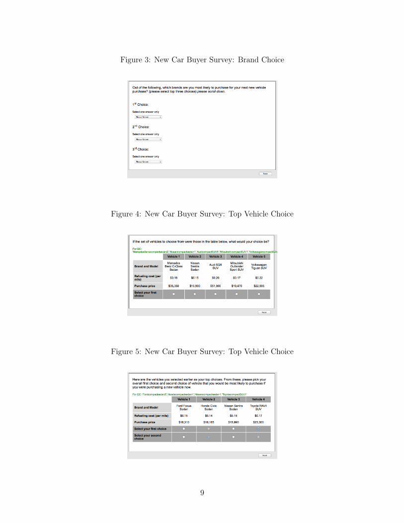
Figure 3: New Car Buyer Survey: Brand Choice

Figure 4: New Car Buyer Survey: Top Vehicle Choice

Figure 5: New Car Buyer Survey: Top Vehicle Choice

9

Figure 6: New Car Buyer Survey: PEV vs. Conventional Vehicle Choice Module

design, we specify Bayesian priors. That is, for each coefficient that we seek to estimate,

we specify an assumed a priori distribution. We base these assumptions on parameter

estimates from earlier studies looking at PEV attributes (Bunch et al., 1993; Golob et al.,

1993; Brownstone, Bunch, and Train, 2000; Ewing and Sarigöllü, 2000; Hidrue et al., 2011;

Qian and Soopramanien, 2011; Achtnicht, Bühler, and Hermeling, 2012).

To make the choice experiment more realistic for respondents, we employ a pivot design.

Price levels are designed to be percentages of a reference value. The price of the top con-

ventional vehicle chosen by a respondent becomes her reference price, and the different price

levels she sees are the percentage levels as specified by the experimental design multiplied

by the reference price. For example, a respondent who selects a conventional model that

costs $30,000 would see BEV and PHEV versions of that model that cost $31,500, $34,500,

$37,500, or $45,000. On the other hand, a respondent who is considering the luxury end of

the market and selects a conventional model that costs $60,000 would see BEV and PHEV

versions of that model that cost $63,000, $69,000, $75,000, or $90,000.

To incorporate the pivoting price attribute levels in the experimental design, NGENE’s

algorithm uses relative attribute levels rather than absolute attribute levels for price. How-

10

Table 2: Attribute Levels

Purchase Price1 (% of conventional)Gasoline 100%BEV 105%, 115%, 125%, 150%PHEV 105%, 115%, 125%, 150%Gasoline Refuel Cost ($ per gal)Gasoline2 $4.00, $4.40, $4.80, $5.60BEV n/aPHEV3 $2.00, $2.20, $2.40, $2.80Electric Refuel Cost4 ($ per gal equivalent)Gasoline n/aBEV $0.90, $1.10, $1.50, $2.50PHEV $0.90, $1.10, $1.50, $2.50Gasoline Range (miles)Gasoline 300BEV 300PHEV 0Electric Range (miles)Gasoline n/aBEV 50, 75, 100, 200PHEV 10, 20, 40, 60HOV AccessGasoline noBEV no, yesPHEV no, yes

1The respondent sees price in dollars. For example, a respondent who selected a conventional model that costs $30,000 wouldsee BEV and PHEV versions of that model that cost $31,500, $34,500, $37,500, or $45,000.2At the time the survey was administered, average gasoline cost in California was approximately $4 per gallon.3The average gasoline fuel economy of PHEVs as of December 2013 was 41mpg, which is roughly double the fuel economy ofour gasoline vehicle universe of 20mpg. Therefore we choose a baseline gasoline refueling cost for PHEVs that is half that ofgasoline vehicles.4At the time the survey was administered, the average overnight electricity rate in California was roughly 16 cents per kWh andthe average vehicle economy of electric vehicles was 3.5 miles per kWh, suggesting an average cost per electric mile of $0.046.The average cost per mile of gasoline vehicles in our vehicle universe is $4/gal

20mi/gal= $0.20 per mile. Thus on average, refueling

cost for electric miles is 23% of the $4 per gallon refueling cost for gasoline miles, or $0.92/gal. Therefore we choose a baselineelectric refueling cost of $0.90 per gallon equivalent.

11

ever, in calculating the efficiency of the design, the algorithm must assume some reference

level. Therefore, we assume four different segments: 1) economy and compact cars, 2) mid-

size and large cars, 3) SUVs, trucks, and minivans, and 4) luxury vehicles. For each segment

we assume the price is the average of that vehicle type from the new vehicle universe. The

algorithm utilizes a model averaging approach according to the actual market shares of the

four segments.

Table A.1 in the Appendix gives definitions of all the variables used in our analysis.

Most of these variables were collected in the survey. We obtained average gasoline prices

in December 2013 by Census Tract from Gas Buddy Organization Inc. From the U.S.

Department of Energy’s Alternative Fuels Data Center we obtained a measure of publicly-

available PEV charger density, which we define as the number of level 2 chargers within a

5-mile radius of the population centroid of a Census Tract as of December 2013.

3 Model Specification

The standard multinomial logit can model the probability of selecting a vehicle over other

alternatives. In this model, a respondent selects the vehicle that gives her greater utility than

any other available alternative. The utility of each alternative is a function of its attributes.

The estimated coefficients tell us how a change in each attribute (e.g., an increase in range)

impacts utility.

Individual n receives utility Uni from choosing alternative i:

Uni = Vni + εni. (1)

The probability of individual n selecting alternative i is the probability her utility from

i is greater than her utility from choosing any other available alternative:

πni = Prob (Vni + εni ≥ Vnj + εnj) ;∀j 6= i. (2)

12

If we assume εni’s are independently distributed Type-I extreme value errors and a linear

utility function, such that Vni = x′iβ, where xi is a vector of attributes of i and β is a vector

of parameters, then we can model the probability of individual n choosing alternative i as:

πni =exp(µnx

′iβ)

J∑j=1

exp(µnx′jβ)

, (3)

where µn is a scale parameter commonly assumed to equal 1.

In this model, the coefficients are fixed, effectively assuming that all respondents have

the same preferences (e.g., all respondents have the same value for a BEV, all else being

equal). The logit model exhibits the independence of irrelevant alternatives (IIA), meaning

that the odds of choosing vehicle j over vehicle k are independent of the choice set for all

pairs j, k, which may imply unrealistic substitution patterns. The standard logit model does

not allow for heterogeneity of preferences.

The first model we estimate that relaxes this assumption is a mixed logit. In the mixed

logit model, developed by Train (1998), the coefficients of the utility function are random

parameters for which we can specify a distribution. For example, if we assume a coefficient is

normally distributed, we estimate both the mean and standard deviation of that coefficient.

This model allows for heterogeneous preferences across respondents and does not necessarily

exhibit the IIA property, thereby allowing for more flexible substitution patterns. Struc-

turally, the mixed logit model is similar to the standard logit except the parameters of the

utility function are assumed to be random, not fixed, and the probability of individual n

selecting alternative i becomes:

πni =

∫exp(µnx

′iβ)

J∑j=1

exp(µnx′jβ)

f (β|θ)∂β, (4)

where f (β|θ) is the density function of β.

A drawback of the mixed logit model is that it does not tell us where different respondents

13

are in the estimated distribution of preferences.5 In other words, it does not tell us which

respondents have which preferences.

The alternative specific constant (ASC) logit and the latent class logit offer two different

methods of further exploring heterogeneity. The ASC logit, developed by McFadden (1974),

is a constant parameter logit where explanatory variables in the utility function include not

only alternative attributes but also respondent characteristics. The ASC logit estimation

therefore tells us how respondent characteristics impact their odds of selecting a BEV or

PHEV relative to the gasoline version. The ASC logit is similar to the standard logit except

the utility function includes consumer characteristics:

Vni = x′iβ + z′nγ, (5)

where zn is a vector of characteristics of individual n and γ is a vector of parameters.

The latent class model is similar to the ASC logit model in that preferences are hetero-

geneous across respondents characteristics. The latent class model segments the population

into different classes, where preferences for each class are estimated separately, and class

membership of respondents is determined by their characteristics.

Assume existence of S segments in a population. The probability of consumer n choosing

alternative i conditional on membership in segment s, where s=1,..,S, is:

πni|s =exp(x′iβs)J∑

j=1

exp(x′jβs)

. (6)

Allowing latent membership for segmentation to be:

M∗ns = y′nλs + ζns, (7)

5Technically, it is possible to make the mean or variance of a mixed logit parameter a function of observedcovariates, but in practice this is rarely done to problems because such models tend to be numerically unstableand frequently do not converge to a well-defined maximum value.

14

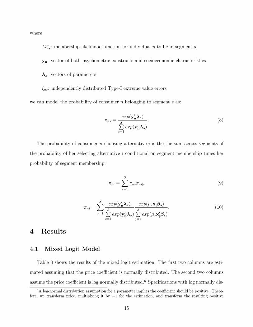
where

M∗ns: membership likelihood function for individual n to be in segment s

yn: vector of both psychometric constructs and socioeconomic characteristics

λs: vectors of parameters

ζns: independently distributed Type-I extreme value errors

we can model the probability of consumer n belonging to segment s as:

πns =exp(y′nλs)S∑

s=1

exp(y′nλs)

. (8)

The probability of consumer n choosing alternative i is the the sum across segments of

the probability of her selecting alternative i conditional on segment membership times her

probability of segment membership:

πni =S∑

s=1

πnsπni|s (9)

πni =S∑

s=1

exp(y′nλs)S∑

s=1

exp(y′nλs)

exp(µsx′iβs)

J∑j=1

exp(µsx′jβs)

. (10)

4 Results

4.1 Mixed Logit Model

Table 3 shows the results of the mixed logit estimation. The first two columns are esti-

mated assuming that the price coefficient is normally distributed. The second two columns

assume the price coefficient is log normally distributed.6 Specifications with log normally dis-6A log-normal distribution assumption for a parameter implies the coefficient should be positive. There-

fore, we transform price, multiplying it by −1 for the estimation, and transform the resulting positive

15

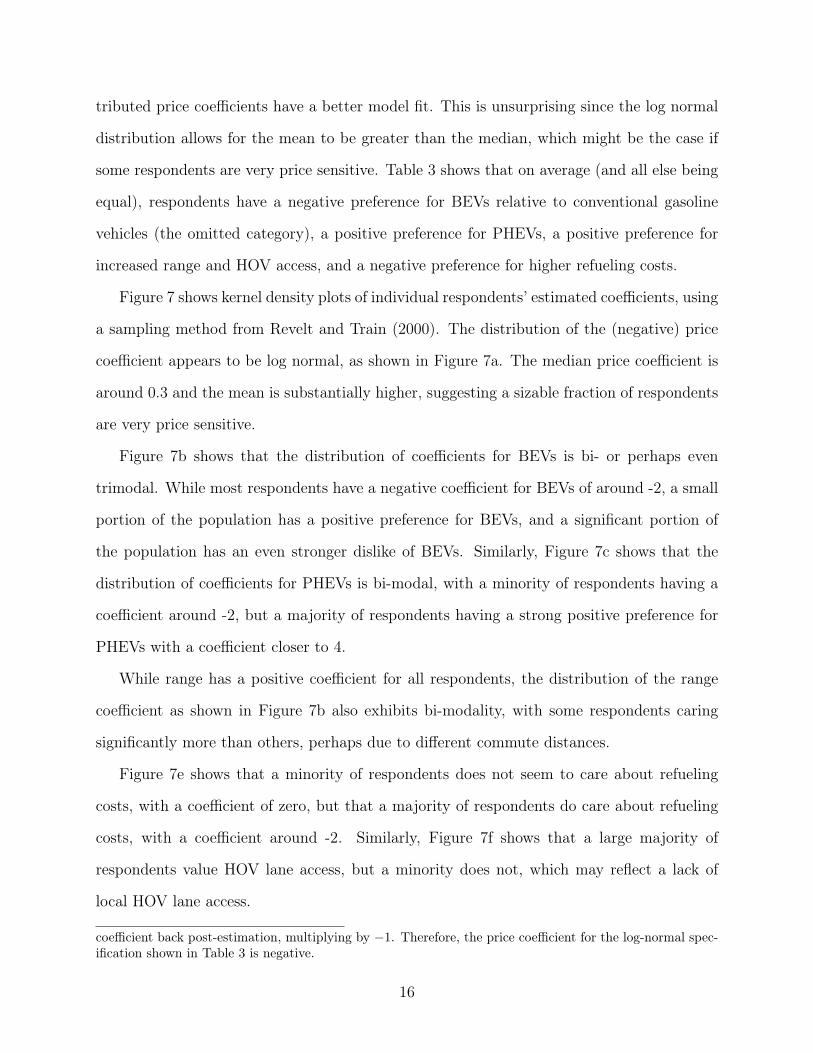
tributed price coefficients have a better model fit. This is unsurprising since the log normal

distribution allows for the mean to be greater than the median, which might be the case if

some respondents are very price sensitive. Table 3 shows that on average (and all else being

equal), respondents have a negative preference for BEVs relative to conventional gasoline

vehicles (the omitted category), a positive preference for PHEVs, a positive preference for

increased range and HOV access, and a negative preference for higher refueling costs.

Figure 7 shows kernel density plots of individual respondents’ estimated coefficients, using

a sampling method from Revelt and Train (2000). The distribution of the (negative) price

coefficient appears to be log normal, as shown in Figure 7a. The median price coefficient is

around 0.3 and the mean is substantially higher, suggesting a sizable fraction of respondents

are very price sensitive.

Figure 7b shows that the distribution of coefficients for BEVs is bi- or perhaps even

trimodal. While most respondents have a negative coefficient for BEVs of around -2, a small

portion of the population has a positive preference for BEVs, and a significant portion of

the population has an even stronger dislike of BEVs. Similarly, Figure 7c shows that the

distribution of coefficients for PHEVs is bi-modal, with a minority of respondents having a

coefficient around -2, but a majority of respondents having a strong positive preference for

PHEVs with a coefficient closer to 4.

While range has a positive coefficient for all respondents, the distribution of the range

coefficient as shown in Figure 7b also exhibits bi-modality, with some respondents caring

significantly more than others, perhaps due to different commute distances.

Figure 7e shows that a minority of respondents does not seem to care about refueling

costs, with a coefficient of zero, but that a majority of respondents do care about refueling

costs, with a coefficient around -2. Similarly, Figure 7f shows that a large majority of

respondents value HOV lane access, but a minority does not, which may reflect a lack of

local HOV lane access.

coefficient back post-estimation, multiplying by −1. Therefore, the price coefficient for the log-normal spec-ification shown in Table 3 is negative.

16

Table 4 shows the mean estimates of willingness to pay (WTP) for vehicle attributes

obtained using the Hensher and Greene approach (Hensher and Greene, 2003).7 We find

that the average WTP for a BEV is about -$4,900. Out of current BEVs on the market as of

early 2014 that have a comparable internal combustion engine (ICE) model, the BEVs are

priced at an average premium of $18,411 (see Table 5 for details). We find that the average

WTP for a PHEV is nearly $6,800. Out of PHEVs on the market as of early 2014 that have a

comparable ICE model, the PHEVs are priced at an average premium of $11,024 (see Table 5

for details). This suggests that the gap between WTP and the price premium for BEVs is

very high, on the order of $23,000, while the gap between WTP and the price premium for

PHEVs is much smaller, on the order of $4,000. State level incentives are typically a few

thousand dollars, and the federal income tax incentive is up to $7,500. This suggests that

current financial incentives will stimulate fewer BEV purchases, but could stimulate more

PHEV purchases. This is consistent with DeShazo, Sheldon, and Carson’s (2015) finding

that California’s PEV rebate policy induces more marginal PHEV purchases than marginal

BEV purchases.

The average survey respondent would pay approximately $589 per year on refueling costs

per $1 increase in $/gal equivalent. This is based on the assumption that the respondent

refuels once every week and a half, and that the respondent’s fuel tank capacity is 17 gallons.

These are the average values based on the survey responses. Thus, the WTP for refuel savings

of $1 per gallon of $430 implies a high discount rate, with an expected payback period of

just under one year.

We find that the average respondent is willing to pay about $900 for free single-occupant

HOV lane access. Bento et al. (2014) estimate the average annual rent of a hybrid HOV

sticker in southern California to be $743, with a net present value of $4,800. Shewmake

and Jarvis (2014) estimate an average premium of $3,200 for a hybrid with an HOV sticker,

7To calculate the mean WTP for each attribute, we took the mean of 10,000 random draws from thedistribution of the attribute’s coefficient divided by the exponential of a random draw from the distributionof the price coefficient.

17

which translates into a yearly value of $625.

The mixed logit results show that there is considerable heterogeneity in preferences across

BEVs and PHEVs, as well as across consumers. Sections 4.2 and 4.3 attempt to better

understand the underlying sources of this heterogeneity.

Table 3: Mixed Logit Results

Price Normally Distributed Price Log Normally DistributedMean Standard Deviation Mean Standard Deviation

Price ($1,000) -0.226*** 0.194** -2.520*** 0.397(0.028) (0.089) (0.257) (0.320)

BEV -1.301** 4.007*** -1.605*** 4.348***(0.656) (0.950) (0.460) (0.817)

PHEV 1.738** 2.745*** 1.921*** 2.423***(0.772) (0.461) (0.407) (0.428)

Range 0.014*** 0.004 0.017*** 0.007***(0.002) (0.003) (0.002) (0.002)

Refuel -0.158** 0.057 -0.128 0.005(0.072) (1.095) (0.096) (0.240)

HOV 0.311** 0.302 0.261*** 0.400**(0.128) (0.753) (0.087) (0.159)

Observations 24,940 24,940Log Pseudolikelihood -5,959 -5,931

Weighted to represent population of California new car buyersRobust standard errors in parentheses, clustered by respondent

*** p<0.01, ** p<0.05, * p<0.1

4.2 Alternative-Specific Constant Logit Model

Tables 6 and 7 show the results of the ASC logit estimation. The coefficient on price in

Table 6, -.06, is smaller in absolute value than the -2.5 estimated by the preferred specification

in Table 3. The former estimate assumes the coefficient is fixed, while the latter estimate

assumes the coefficient follows a log normal distribution and allows for the mean to be

greater than the median, which might be the case due to a small fraction of respondents

18

(a) (b)

(c) (d)

(e) (f)

Figure 7: Mixed Logit Coefficient Distributions

19

Table 4: Willingness to Pay

WTP WTP(Price (Price Log

Normally Distributed) Normally Distributed)BEV -$18,693 -$4,906

PHEV $12,873 $6,783

Additional Mile of $81 $57Electric Range

Additional $ per Gal -$874 -$430Refuel Cost

HOV Access $1,555 $903

Table 5: Price Comparison of Internal Combustion Engine (ICE) vehicles and PEVs of theSame Model

ICE MSRP BEV MSRP PremiumSmart for Two $13,270 $25,000 $11,730Chevrolet Spark $12,170 $26,685 $14,515Ford Focus $16,810 $35,170 $18,360Toyota RAV4 $23,550 $49,800 $26,250Honda Fit $15,425 $36,625 $21,200Avg Premium $18,411

ICE MSRP PHEV MSRP PremiumFord C-Max $25,170 $32,920 $7,750Ford Fusion $21,970 $34,700 $12,730Honda Accord $21,955 $39,780 $17,825Toyota Prius Plug-In $24,200 $29,990 $5,790Avg Premium $11,024MSRPs are taken from auto makers’ websites and www.edmunds.com. MSRPs as of March 2014.

20

being very price sensitive. The coefficients on refueling costs and HOV access are similar

between Tables 3 and 6. The BEV and PHEV coefficients are not directly comparable, as

those in Table 6 must be adjusted by respondent characteristics as shown in Table 7. For

example, the coefficient on Gas Price in Table 7 is approximately 1.5, and the gas price

in most Census Tracts during December of 2013 was greater than $3, such that at least

3 ∗ 1.5 = 4.5 must be added to both the BEV and PHEV coefficients in Table 6.

Table 6: Alternative-Specific Constant Logit, Main Results

Price ($1,000s) -0.062***(0.009)

BEV -9.701****(3.604)

PHEV -8.936***(2.701)

Range 0.033***(0.003)

Range2 -0.0001***(.00001)

Refuel -0.086**(0.045)

HOV 0.239***(0.057)

Observations 24,620Log Pseudolikelihood -6,732Weighted to represent population of California new car buyersRobust standard errors in parentheses, clustered by respondent

*** p<0.01, ** p<0.05, * p<0.1

Due to the complexity of the model, we are unable to achieve convergence in the max-

imum likelihood estimation of the mixed logit when we include a quadratic range term in

the specification. We are able to achieve convergence in the ASC logit estimation when a

quadratic range term is included. When we include this term, we get more precision on the

refueling cost coefficient and we find that consumers’ utility for range exhibits decreasing

returns. This is consistent with the literature (Bunch et al., 1993; Brownstone, Bunch, and

Train, 2000). The linear and quadratic range coefficients suggest an optimal electric range

21

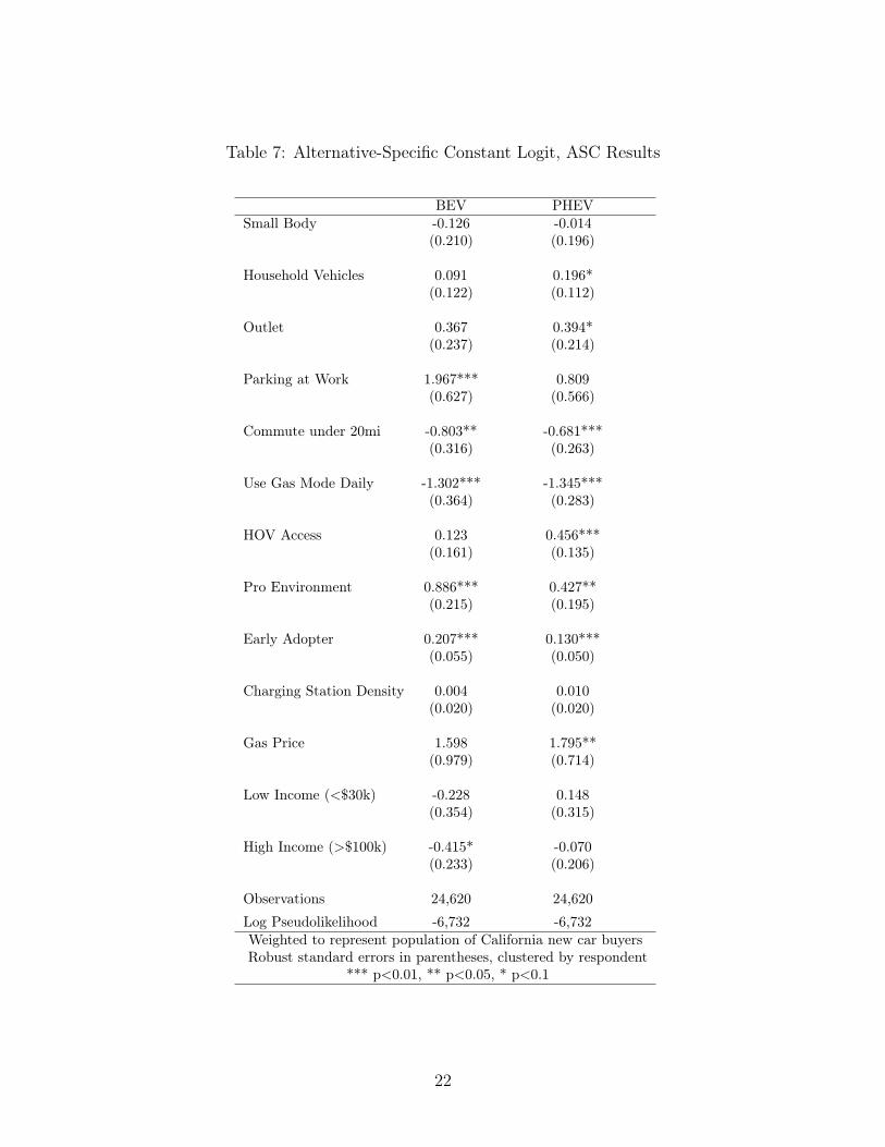
Table 7: Alternative-Specific Constant Logit, ASC Results

BEV PHEVSmall Body -0.126 -0.014

(0.210) (0.196)

Household Vehicles 0.091 0.196*(0.122) (0.112)

Outlet 0.367 0.394*(0.237) (0.214)

Parking at Work 1.967*** 0.809(0.627) (0.566)

Commute under 20mi -0.803** -0.681***(0.316) (0.263)

Use Gas Mode Daily -1.302*** -1.345***(0.364) (0.283)

HOV Access 0.123 0.456***(0.161) (0.135)

Pro Environment 0.886*** 0.427**(0.215) (0.195)

Early Adopter 0.207*** 0.130***(0.055) (0.050)

Charging Station Density 0.004 0.010(0.020) (0.020)

Gas Price 1.598 1.795**(0.979) (0.714)

Low Income (<$30k) -0.228 0.148(0.354) (0.315)

High Income (>$100k) -0.415* -0.070(0.233) (0.206)

Observations 24,620 24,620

Log Pseudolikelihood -6,732 -6,732Weighted to represent population of California new car buyersRobust standard errors in parentheses, clustered by respondent

*** p<0.01, ** p<0.05, * p<0.1

22

of 165 miles.

Table 6 shows that all else being equal, consumers prefer PHEVs to BEVs. Table 7 shows

that having pro environment preferences and self-identifying as an early adopter increase a

respondent’s WTP for both BEVs and PHEVs, although relatively more for BEVs.

Respondents with round-trip commutes under 20 miles are less likely to select PEVs.

This may be because a shorter commute would accrue less refueling cost savings, making it

more difficult for the consumer to justify the higher upfront cost of a PEV.

The environmental benefits associated with driving a PHEV depend on the relative num-

ber of miles driven in electric versus gasoline mode. While the California Air Resources

Board currently assigns higher rebates to BEVs in the belief they are associated with greater

environmental benefits than PHEVs, it is sometimes argued that PHEVs may result in close

to the same environmental benefits if daily commuting can be done in all-electric mode

(California Environmental Protection Agency, 2007). PHEVs do not invoke range anxiety

or impair the ability to take longer occasional trips. The results in Table 7 support this

assertion. Respondents who anticipate needing to utilize gasoline mode on a daily basis if

they owned a PHEV are much less likely to purchase either a BEV or a PHEV. This effect is

similar for BEVs and PHEVs, suggesting prospective PHEV drivers are equally as motivated

to commute primarily in all-electric mode, even though they do not face the same total range

constraints as BEVs.

The positive coefficients on outlet access in Table 7 suggest that respondents who have

an electrical outlet near their home parking spot are more likely to purchase a PEV. This is

consistent with earlier studies (Axsen and Kurani, 2009; Hidrue et al., 2011). Notably, outlet

access appears just as important for PHEVs as BEVs, even though PHEVs do not require

the electric battery be charged in order to drive the vehicle in gasoline mode. However, when

we replace the outlet variable with an indicator variable for whether the respondent lives

in a single-family house, this coefficient is positive and statistically significant at the 10%

23

level for BEVs but smaller and not statistically different from zero for PHEVs.8 This may

suggest that BEV owners are more comfortable plugging into an outlet at their single family

residence while PHEV owners living in multifamily housing are also comfortable plugging

into a less private or less exclusive outlet near their residential parking spot.

The coefficient on the indicator for whether a respondent parks in a garage while at

work is positive and highly statistically significant for BEVs but smaller and not significant

for PHEVs. Respondents with access to a parking garage at work may anticipate a higher

likelihood of charging access while at work, which would increase their utility for PEVs. These

coefficients suggest that workplace charging is a more important issue for BEV adoption

than PHEV adoption. The coefficients on public charging station density are positive but

not statistically different from zero.

The coefficients on HOV lane access are positive, but that for BEVs is smaller than that

for PHEVs and not statistically significant. This suggests that new car buyers who live

near HOV lanes are more likely to purchase PHEVs, and that government policies allowing

free single-occupant HOV lane access increase consumer probability of purchasing PHEVs.

Sheldon and DeShazo (2015) find that California’s HOV lane policy had a positive impact

on both BEV and PHEV adoption, with relatively more impact on the PHEV market.

The coefficient on number of household vehicles is positive for both vehicle types, although

only statistically significantly greater than zero for PHEVs. This lends support to the “Hybrid

Household” hypothesis that households with larger vehicle fleets are more likely to diversify

their vehicle holdings with alternative vehicles (Kurani, Turrentine, and Sperling, 1996).

The coefficients on small body type are not statistically different from zero, implying that

respondents who are likely to purchase a new vehicle that is a hatchback or small sedan are

neither more nor less likely than other respondents to select a PEV. Although the majority

of PEVs on the market have historically been smaller vehicles, this result is unsurprising

8If we substitute the Outlet variable with Single House, the BEV coefficient on Single House is 0.427*(0.234) and the PHEV coefficient on Single House is 0.151 (0.207), with other coefficients not significantlydifferent. We do not include Outlet and Single House in the same specification due to concerns aboutcollinearity.

24

because in our choice experiment, respondents were allowed to choose PEV versions of any

body type.

4.3 Latent Class Model

Tables 8 and 9 show the results of a latent class estimation assuming three segments, using

a variety of sociodemographic variables and attitudes to determine segment membership.

Note that the latent class groups are helpful in explaining the kernel density estimate of

coefficients. For example, Figure 7b shows that there are three peaks in the BEV coefficient

distribution: one at a large negative number, the biggest at a small negative number, and

the third and smallest peak at a near-zero positive number. These three peaks are consistent

with the three BEV preferences of the different segments.

Table 8: Latent Class Model: Segment Preferences

Segment 1 Segment 2 Segment 3

Price ($1,000s) -0.193*** -0.387*** -0.024***(0.016) (0.052) (0.007)

BEV -3.752*** -3.031*** -0.197(0.382) (0.485) (0.300)

PHEV 0.643** -1.531*** 0.511**(0.298) (0.403) (0.251)

Range 0.051*** 0.013** 0.018***(0.003) (0.006) (0.003)

Range2 -0.0002*** -.00003 -.00003***(0.00002) (0.00002) (0.00001)

Refuel -0.219*** -0.088 -0.123**(0.073) (0.105) (0.052)

HOV 0.382*** -0.073 0.232***(0.089) (0.156) (0.064)

Class Share 42.4% 26.1% 31.5%Observations 24,940 24,940 24,940

Standard errors in parentheses*** p<0.01, ** p<0.05, * p<0.1

25

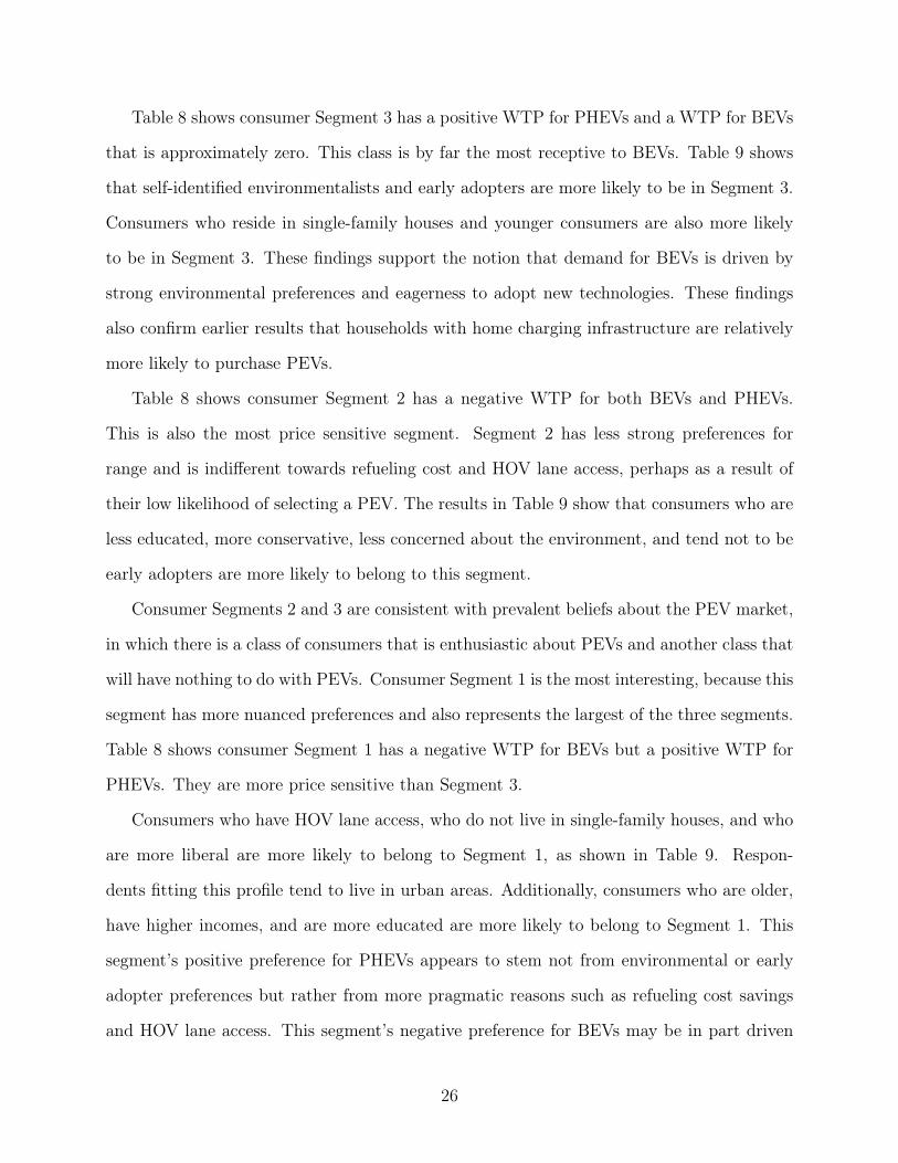
Table 8 shows consumer Segment 3 has a positive WTP for PHEVs and a WTP for BEVs

that is approximately zero. This class is by far the most receptive to BEVs. Table 9 shows

that self-identified environmentalists and early adopters are more likely to be in Segment 3.

Consumers who reside in single-family houses and younger consumers are also more likely

to be in Segment 3. These findings support the notion that demand for BEVs is driven by

strong environmental preferences and eagerness to adopt new technologies. These findings

also confirm earlier results that households with home charging infrastructure are relatively

more likely to purchase PEVs.

Table 8 shows consumer Segment 2 has a negative WTP for both BEVs and PHEVs.

This is also the most price sensitive segment. Segment 2 has less strong preferences for

range and is indifferent towards refueling cost and HOV lane access, perhaps as a result of

their low likelihood of selecting a PEV. The results in Table 9 show that consumers who are

less educated, more conservative, less concerned about the environment, and tend not to be

early adopters are more likely to belong to this segment.

Consumer Segments 2 and 3 are consistent with prevalent beliefs about the PEV market,

in which there is a class of consumers that is enthusiastic about PEVs and another class that

will have nothing to do with PEVs. Consumer Segment 1 is the most interesting, because this

segment has more nuanced preferences and also represents the largest of the three segments.

Table 8 shows consumer Segment 1 has a negative WTP for BEVs but a positive WTP for

PHEVs. They are more price sensitive than Segment 3.

Consumers who have HOV lane access, who do not live in single-family houses, and who

are more liberal are more likely to belong to Segment 1, as shown in Table 9. Respon-

dents fitting this profile tend to live in urban areas. Additionally, consumers who are older,

have higher incomes, and are more educated are more likely to belong to Segment 1. This

segment’s positive preference for PHEVs appears to stem not from environmental or early

adopter preferences but rather from more pragmatic reasons such as refueling cost savings

and HOV lane access. This segment’s negative preference for BEVs may be in part driven

26

Table 9: Latent Class Model: Segment Membership

Segment 1 Segment 2 Segment 3†

Household Size -0.049 -0.238*** 0.000(0.070) (0.077)

Household Vehicles 0.231** 0.172 0.000(0.106) (0.113)

Age under 35 -0.648*** -0.305 0.000(0.205) (0.217)

Age over 60 0.548** 0.504* 0.000(0.255) (0.258)

Low Income (<$30k) 0.322 0.108 0.000(0.262) (0.267)

High Income (>$100k) 0.349* 0.074 0.000(0.211) (0.225)

College Education 0.056 -0.290 0.000(0.187) (0.197)

Use Gas Mode Daily 0.005 0.793** 0.000(0.382) (0.357)

Single House -0.398** -0.313 0.000(0.194) (0.204)

HOV Access 0.050 -0.436*** 0.000(0.121) (0.133)

Pro Environment -0.641*** -1.088*** 0.000(0.175) (0.191)

Early Adopter -0.077* -0.219*** 0.000(0.046) (0.049)

Liberal 0.332* -0.017 0.000(0.189) (0.212)

Constant 0.277 1.439*** 0.000(0.405) (0.407)

Class Share 42.4% 26.1% 31.5%Observations 24,940 24,940 24,940

Standard errors in parentheses*** p<0.01, ** p<0.05, * p<0.1

†Segment 3 is the baseline segment that the other segments are compared to.

27

by less access to home charging.

The latent class results show that the BEV market may be constrained since less than a

third of the new car buying population seems willing to consider purchasing a BEV, all else

being equal. A much larger fraction of the population, and one that breaks out of the early

adopter/environmentalist niche, seems willing to consider purchasing a PHEV.

5 Implications for Policy and the Emerging Market

Results from the mixed logit model suggest that the gap between WTP and the price

premium for BEVs is very high, on the order of $23,000, while the gap between WTP and

the price premium for PHEVs is much smaller, on the order of $4,000. This suggests that

financial incentives of a few thousand dollars, similar to current subsidy levels, will stimulate

fewer BEV purchases, but could stimulate more PHEV purchases.

In the ASC logit model we find that consumers’ utility for range exhibits decreasing

returns. The linear and quadratic range coefficients suggest an optimal electric range of 165

miles. A similar calculation for the latent class model suggests optimal ranges for Segment

1, 2 and 3 of 127.5, 216.7, and 300 miles, respectively. Segment 3 is the most likely to

choose a BEV and is the least price sensitive, so it makes sense this segment is willing to

pay for a longer range. Segment 1 is more likely to purchase a PHEV, such that a more

cost-effective, shorter range vehicle may be sufficient. In the ASC logit model we also find

evidence that prospective PHEV drivers are equally as motivated to commute primarily in

all-electric mode, even though they do not face the same total range constraints as BEVs.

In the mixed logit model, we find that the average respondent is willing to pay about

$900 for free single-occupant HOV lane access. In the ASC logit model, the coefficients on

HOV lane access are positive, but that for BEVs is smaller than that for PHEVs and not

statistically significant. This suggests that new car buyers who live near HOV lanes are more

likely to purchase PHEVs, and that government policies allowing free single-occupant HOV

28

lane access increases consumer probability of purchasing PHEVs.

In the ASC logit model we find that charging close to home access appears just as

important for PHEVs as BEVs, even though PHEVs do not require the electric battery to

be charged in order to drive the vehicle in gasoline mode. These results suggest that home

charging is just as important to consumers considering a PHEV purchase. However, we

also find evidence that BEV owners are more comfortable plugging into an outlet at their

single family residence while PHEV owners living in multifamily housing are also comfortable

plugging into a less private or less exclusive outlet near their residential parking spot. Our

latent class model similarly suggests that consumers living in a single-family household are

more likely to purchase BEVs. In the ASC logit model we also find evidence that the ability

to charge at work is more important for BEV adoption than PHEV adoption.

The latent class model reveals three distinct consumer segments. About a quarter of the

new car buyer population seems to be less urban, more conservative, and have strong negative

preferences for all PEVs. A third of the population has pro-environmental preferences and a

tendency for early adoption. This is the only segment that does not have a strong negative

preference for BEVs. The last segment, Segment 1, tends to be more urban, older, higher

income, and more educated. These consumers have a strong negative preference for BEVs

but a strong positive preference for PHEVs. This positive preference for PHEVs appears not

to stem from environmental or early adopter preferences. This segment’s negative preference

for BEVs may be in part driven by less access to home charging.

The latent class results show that the BEV market may be constrained since less than a

third of the new car buying population seems willing to consider purchasing a BEV, all else

being equal. On the other hand, a much larger and more general population seems willing to

consider purchasing a PHEV and even has a positive willingness to pay for this technology

relative to a conventional gasoline vehicle. This suggests that the addition of PHEVs to

the market may stimulate PEV demand in consumer segments who would otherwise be

unlikely to purchase a BEV. These findings also imply that many PHEV purchasers would

29

not purchase a BEV, and such sales would represent growth in the overall PEV market rather

than cannibalization of the BEV market. We speculate that due to the strong negative

preferences for BEVs in most of the population and cost differentials that are large relative

to subsidy levels being considered by policy makers, much of the future growth of the PEV

market will be driven by demand for PHEVs from Segment 1.

30

References

Achtnicht, Martin, Georg Bühler, and Claudia Hermeling (2012), “The impact of fuel avail-

ability on demand for alternative-fuel vehicles,” Transportation Research Part D, 17: 262-

269.

Axsen, Jonn, and Kenneth S. Kurani (2009), “Early US market for plug-in hybrid electric

vehicles,” Transportation Research Record: Journal of the Transportation Research Board

2139, no. 1: 64-72.

Axsen, John and Kenneth S. Kurani (2013), “Hybrid, plug-in hybrid, or electric-What do

car buyers want?,” Energy Policy, 61: 532-543.

Bento, Antonio, Daniel Kaffine, Kevin Roth, and Matthew Zaragoza-Watkins (2014), “The

effects of regulation in the presence of multiple unpriced externalities: Evidence from the

transportation sector,” American Economic Journal: Economic Policy, 6(3): 1-29.

Brownstone, David, David S. Bunch, and Kenneth Train (2000), “Joint mixed logit models

of stated and revealed preferences for alternative-fuel vehicles,” Transportation Research

Part B, 34: 315-338.

Bunch, David S., Mark Bradley, Thomas F. Golob, Ryuichi Kitamura, and Gareth P. Oc-

chiuzzo (1993), “Demand for clean-fuel vehicles in California: A discrete-choice stated

preference pilot project,” Transportation Research Part A, 27A(3): 237-253.

California Environmental Protection Agency (2007), Status report on the California Air

Resources Board’s Zero Emission Vehicle Program.

Caperello, Nicolette D. and Kenneth S. Kurani (2012), “Households’ stories of their encoun-

ters with a plug-in hybrid electric vehicle,” Environment and Behavior, 44(4): 493-508.

DeShazo, J.R., Tamara L. Sheldon and Richard T. Carson (2015), “Designing policy in-

centives for cleaner technologies: Lessons from California’s plug-in electric vehicle rebate

31

program,” Working Paper, Luskin School of Public Affairs, University of California, Los

Angeles.

Ewing, Gordon and Emine Sarigöllü (2000), “Assessing consumer preferences for clean-fuel

vehicles: A discrete choice experiment,” Journal of Public Policy and Marketing, 19(1):

106-118.

Egbue, Ona, and Suzanna Long (2012), “Barriers to widespread adoption of electric vehicles:

An analysis of consumer attitudes and perceptions,” Energy Policy, 48: 717-729.

Golob, Thomas F., Ryuichi Kitamura, Mark Bradley, and David S. Bunch (1993), “Predict-

ing the market penetration of electric and clean-fuel vehicles,” The Science of the Total

Environment, 134: 371-381.

Graham-Rowe, Ella, Benjamin Gardner, Charles Abraham, Stephen Skippon, Helga

Dittmar, Rebecca Hutchins, and Jenny Stannard (2012), “Mainstream consumers driving

plug-in battery-electric and plug-in hybrid electric cars: A qualitative analysis of responses

and evaluations,” Transportation Research Part A, 46: 140-153.

Hensher, David A. and William H. Greene (2003), “The Mixed Logit model: The state of

practice,” Transportation, 30:133-176.

Hidrue, Michael K., George R. Parsons, Willett Kempton, and Meryl P. Gardner (2011),

“Willingness to pay for electric vehicles and their attributes,” Resource and Energy Eco-

nomics, 33: 686-705.

Khan, Mobashwir, and Kara M. Kockelman (2012), “Predicting the market potential of

plug-in electric vehicles using multiday GPS data,” Energy Policy, 46: 225-233.

Kurani, Kenneth S., Reid R. Heffner, and Tom Turrentine (2008),“Driving plug-in hybrid

electric vehicles: Reports from US drivers of HEVs converted to PHEVs, circa 2006-07,”

Institute of Transportation Studies.

32

Kurani, Kenneth S., Thomas Turrentine, and Daniel Sperling (1996), “Testing electric vehicle

demand in ’hybrid households’ using a reflexive survey,” Transportation Research Part D,

1(2): 131-150.

McFadden, Daniel (1974), “Conditional logit analysis of qualitative choice behaviour,” in

Frontiers in Econometrics, edited by P. Zarembka (New York: Academic Press), pages

105-142.

Qian, Lixian and Didier Soopramanien (2011), “Heterogeneous consumer preferences for

alternative fuel cars in China,” Transportation Research Part D, 16: 607-613.

Revelt, David, and Kenneth Train (2000), “Customer-specific taste parameters and mixed

logit: Households’ choice of electricity supplier,” Working Paper, Department of Eco-

nomics, University of California, Berkeley.

Scarpa, Riccardo, and John M. Rose (2008), “Design efficiency for non-market valuation

with choice modelling: how to measure it, what to report and why,” Australian Journal

of Agricultural and Resource Economics, 52(3): 253-282.

Sheldon, Tamara L., and J.R. DeShazo (2015), “How does the presence of HOV lanes affect

plug-in electric vehicle adoption in California? A generalized propensity score approach,”

Working Paper, Department of Economics, University of South Carolina.

Shewmake, Sharon, and Lovell Jarvis (2014), “Hybrid cars and HOV lanes,” Transportation

Research Part A, 67: 304-319.

Train, Kenneth E. (1998), “Recreation demand models with taste differences over people,

Land Economics, 74(2): 230-239.

33

A Appendix

Table A.1: Definition of Variables

Variable Name Description

BEV Indicator for whether the chosen vehicle is a BEV

PHEV Indicator for whether the chosen vehicle is a PHEV

Range Electric range of chosen vehicle (miles)

Refuel Refueling cost of chosen vehicle ($ per gallon equivalent)

HOV Indicator for whether the chosen vehicle is granted free single-

occupant access to high occupancy vehicle lanes

Small Body Binary variable for if the respondent indicated that the vehicle

she is most likely to select for her next new vehicle purchase is

a compact car, midsize car, or hatchback

Household Size Number of members of household, including respondent

Household Vehicles Number of vehicles in respondent’s household

Age under 35 Binary variable for if respondent is less than 35 years old

Age over 60 Binary variable for if respondent is more than 60 years old

Outlet Binary variable that equals 1 if the respondent indicated an

electrical outlet located within 100 feet of her home parking spot

Single House Binary variable for if respondent lives in a one-family house

detached from any other house or a one-family house or condo

attached to one or more houses

Parking at Work Binary variable for if the respondent indicated she parks

her vehicle in a commercial lot or garage while at work

Commute under 20mi Binary variable for if the respondent indicated that the shortest

electric range she would need for daily commute is under 20 miles

Use Gas Mode Daily Binary variable for if the respondent purchased a PHEV, she

anticipates using gasoline mode almost daily

Continued on next page

34

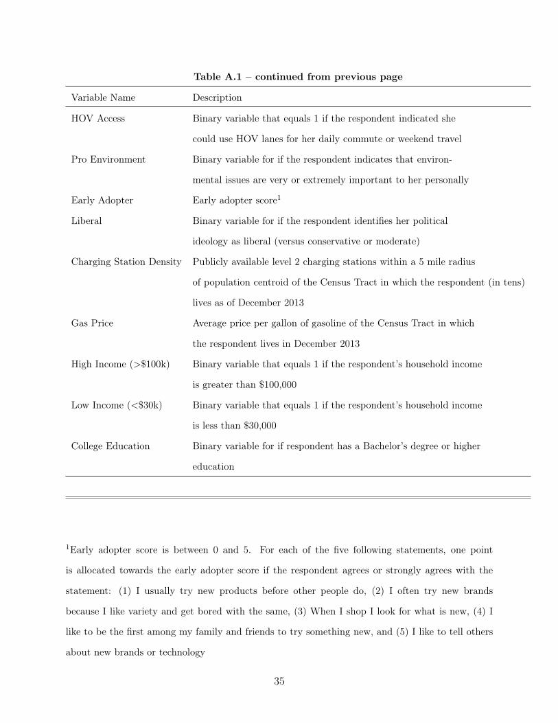
Table A.1 – continued from previous page

Variable Name Description

HOV Access Binary variable that equals 1 if the respondent indicated she

could use HOV lanes for her daily commute or weekend travel

Pro Environment Binary variable for if the respondent indicates that environ-

mental issues are very or extremely important to her personally

Early Adopter Early adopter score1

Liberal Binary variable for if the respondent identifies her political

ideology as liberal (versus conservative or moderate)

Charging Station Density Publicly available level 2 charging stations within a 5 mile radius

of population centroid of the Census Tract in which the respondent (in tens)

lives as of December 2013

Gas Price Average price per gallon of gasoline of the Census Tract in which

the respondent lives in December 2013

High Income (>$100k) Binary variable that equals 1 if the respondent’s household income

is greater than $100,000

Low Income (<$30k) Binary variable that equals 1 if the respondent’s household income

is less than $30,000

College Education Binary variable for if respondent has a Bachelor’s degree or higher

education

1Early adopter score is between 0 and 5. For each of the five following statements, one point

is allocated towards the early adopter score if the respondent agrees or strongly agrees with the

statement: (1) I usually try new products before other people do, (2) I often try new brands

because I like variety and get bored with the same, (3) When I shop I look for what is new, (4) I

like to be the first among my family and friends to try something new, and (5) I like to tell others

about new brands or technology

35