1

This is the unformatted version of: Yeun-Touh, L., Schmöcker, J.-D. and Fujii, S. (2014). Demand

Adaptation towards New Transport Modes: Case of High Speed Rail in Taiwan. Transportmetrica

B. doi: 10.1080/21680566.2014.946456.

Demand Adaptation towards New Transport Modes:

Case of High Speed Rail in Taiwan

Yeun-Touh Li, Jan-Dirk Schmöcker, Satoshi Fujii

Yeun-Touh Li PhD Student, Department of Urban Management,

Graduate School of Engineering, Kyoto University, Japan Address: Room C1-2-437, Katsura Campus, Nishikyo-Ku,

Kyoto, 615-8540, Japan

Phone numbers: +81-80-5770-8002

Fax numbers: +81-075-383-3236

e-mail: joe.liyt@trans.kuciv.kyoto-u.ac.jp

Jan-Dirk Schmöcker Associate Professor, Department of Urban Management,

Graduate School of Engineering, Kyoto University, Japan Address: Katsura Campus, Nishikyo-Ku,

Kyoto, 615-8540, Japan

e-mail: schmoecker@trans.kuciv.kyoto-u.ac.jp

Satoshi Fujii Professor, Department of Urban Management,

Graduate School of Engineering, Kyoto University, Japan Address: Katsura Campus, Nishikyo-Ku,

Kyoto, 615-8540, Japan

e-mail: fujii@trans.kuciv.kyoto-u.ac.jp

2

ABSTRACT

This study aims to explain the factors affecting ridership changes on the relatively new

Taiwan High Speed Rail system (THSR). The analysis is based on monthly ridership data from

January 2007 to December 2013. We also discuss the impact of THSR on competing modes such

as air demand. Econometric time-series models are used for ridership estimation. Firstly a

seasonal autoregressive integrated moving average (SARIMA) model was applied; showing that

the ridership thrives and that the trend prediction fairly well performed if applied to data after

2012. Secondly, to specify the impact of explanatory variables, a first order moving average

model was fitted. Results show that ridership, population and fuel price have a positive effect

while unemployment and car ownership tend to reduce the THSR ridership. We include as

separate factor “month since operation start”, show that this factor is significant and discuss its

relation to demand adaptation. Implications for general equilibrium modelling for new transport

systems are discussed. Moreover, ridership data from two specific stations are used to test the

importance of predominant trip purposes for demand estimation.

Keywords: High Speed Rail; Demand Forecasting; Time Series Modelling; Trend;

Adaptation Effect

3

1. INTRODUCTION: DEMAND FOR NEW PUBLIC TRANSPORT SCHEMES

Demand Forecasting is a key issue for transport planning. Over the last decades various tools

have been developed to assess the impact of network changes on the demand. One can observe

though that generally model accuracy drops the longer the planning horizon. The reasons for this

are obvious in that the uncertainties increase the longer the time horizon. Further, models have

most success to predict the demand for small alterations to existing systems. Demand prediction

for major infrastructure investments are in most cases far more difficult. In some cases demand

estimates have been found to be very far from predictions. A notable recent example is the

demand for the Incheon Airport Express in Korea which is far below model estimates (KMLIT,

2009). An explanation is that demand adaptation is influenced by far more factors than usually

included in utility estimations that are the basis for mode or route choice models.

An additional issue is that the timing of demand adaptation appears often difficult to predict.

Initial demand might be low but only over a fairly long time period the demand might increase to

somewhere near the predicted (user equilibrium) level. Some rail operators for example discount

the demand for the first few years for new services compared to their usual demand prediction

method.

The problem at stake is though that exactly for large infrastructure investments, a planner is in

most need for demand predictions as this is a key factor in project appraisal. For example, initial

demand for the magnetic elevated train considered for construction between Hamburg and Berlin

in Germany were estimated at 14 million passengers per year initially. The estimates were later

downward revised leading eventually to the rejection of the project. Other sustainable transport

policies currently under discussion face similar issues. For example there is a wide range of

predictions for the demand of electric cars (Lieven et al. 2011; Link et al. 2012) and bicycle

sharing (Fishman et al. 2013; DeMaio, 2009). Also a number of public transport systems have

been introduced but services were cancelled after some time when demand did not reach

expectations. On the other hand also positive examples are known where demand exceeded

predictions (Lee and Senior, 2013; Abrate et al. 2009; FitzRoy and Smith, 1998).

Especially the time duration dimension appears to be under researched. When investments aim

to promote mode changes, it is reasonable to assume that potential users need time to adapt their

behaviour. For example Owen and Phillips (1987) distinguish “short-term” and “long-term”

impacts of service changes to railway demand. Therefore the aim of this paper is to discuss

factors that influence the demand development for newly introduced public transportation

schemes. That is, we want to know how long it takes for a new system to reach a constant stable

demand (if ever). In modelling terms we might phrase this as the time it takes for the system to

reach a new equilibrium distribution between the modes (if one exists and if it can be reached).

4

As a case study we analyse the demand for the Taiwanese High Speed Rail System. The service

was introduced in 2007. As will be discussed in the following the service only was altered

significantly in the first year of its operation, after that, until today, service attributes have stayed

fairly constant. Therefore one might assume that the demand will also be stable after a while

which is though not the case. We discuss possible reasons for this as well as general implications

for long term demand forecasting.

The reminder of this paper is organised as follows. Section 2 reviews in more detail potential

factors influencing the demand adaptation in response to public transport investments. Section 3

introduces the case study. Sections 4 and 5 then present a time series analysis of the demand

development. We firstly employ a SARIMA model in Section 4 followed by a simpler MA(1)

model in Section 5 where we introduce explanatory variables discussed in previous sections. In

Section 6 we repeat the analysis of Section 5 with ridership data from two specific stations.

Section 7 concludes this study with a discussion on implications and future extensions.

2. LITERATURE REVIEW: DEMAND ADAPTATION TO NEW PT SERVICES

A number of major factors influencing (long-term) demand adaptation to public transport

investments can be distinguished. For one, obviously by the population perceived quality and

service attributes of the new service will influence the demand as discussed in most of the mode

choice literature. Fares, frequency, travel time, and service reliability (punctuality) generally are

considered as quantitative factors whereas safety concerns, comfort level, and in-vehicle service

are considered as qualitative demand determinants. For example safety records will influence

airline demand over longer time periods (Ito and Lee, 2005) and similarly for new rail systems

passengers whom might need some time to adapt to these and gain trust. Fu et al. (2014) estimate

the demand split between rail and air in Japan if “super high speed rail” is introduced between

Osaka and Tokyo. They suggest that passengers will be sensitive to fare and frequency and that

eventually air might be driven out of the market.

Further, obviously socio-demographics and their developments will influence the demand. In

line with the analysis presented later in this paper, Kyte et al. (1988) used time-series analysis to

examine the factors affecting changes in transit ridership in Portland. One factor they identify is

population size. Similarly, also for large national projects the total population growth should

therefore be considered, especially if more specific market size estimation is not available.

General economic developments measured by GDP and unemployment rate will play a further

role. Important to note are further the cyclic and “endogenous effects” if very large transit

investments are considered, which make it difficult to estimate their total demand as well as the

5

time when the effect will occur. For example, both in developed and developing countries,

Gwilliam (2008) review the development of thought on the major issues in transit economics

over the last half century. He concluded that transit is critical to the achievement of a wide range

of social, economic and environmental objectives. Similarly, Chen (2010) identifies factors that

impact high-speed rail ridership (as well as ticket fares) in the North Eastern parts of the United

States. He suggests that economic factors such as employment in manufacturing seem to be most

significant. Transit investments will trigger further economic investments. They hence create

induced demand and will have an impact on other determinants of transit ridership such as car

ownership. Ahlfeldt and Feddersen (2010) argue that the economic geography framework, such

as population distribution, economic activity density, and spatial development structure, can help

to derive extant predictions on the economic impact of transport projects and vice versa. The

expectation that transport innovations would also lead to sustainable economic growth has long

since motivated public investment into large-scale infrastructure projects. Connected to economic

developments are also gasoline prices. Lane (2012) shows with data from 33 U.S. cities that

gasoline prices have exhibited considerable fluctuation in public transport demand. Further car

ownership is driven by economic developments. Bass et al. (2011) for example reports the

connection between increasing household income and car ownership particularly in developing

countries, with this leads to a significant decline in public transit ridership.

A fourth group of factors which significant for long term demand might be termed “general

perceptions and attitudes”. That is, generally concern for health and environment might have

promoted the use of public transport over the least years. The car seems to lose its meaning as

status symbol over the last years to some degree (Belgiawan et al. 2012). Also, in particular for

new technologies, perceptions of whether the system is safe or convenient will influence demand.

Abrate et al. (2009) analysis the impact of Integrated Tariff Systems (ITS) on public transport

demand in Italy, and indicate that the introduction of such system can increase the number of

passenger trips both in the short-run (2.19%) and long-run (12.04%). FitzRoy and Smith (1998)

investigate the demand of local public transport in Germany; and argue that although traffic

restraint measures and improvements in the quality of the public transit service are significant

factors, the main explanation lies in the introduction of low cost environmental travel cards with

the key characteristics of transferability across friends and family and wide regional validity

across operators. That is, not only the convenience of the card but also the promotion of the

service as environmental might have had an effect. Chao et al. (2012) indicate the concept of

perceived value from public transport is closely linked to customers’ satisfaction. The results

show that the satisfaction value could be identified as social, functional, and emotional value.

However, this group of factors is usually very difficult to include in demand forecasting.

6

A fifth group of factors might be called “direct endogenous factors” (in contrast to other more

indirect factors such as the above discussed economic impacts).That is, through the introduction

of a new system some cyclic effects might be triggered. For example land-use values might

change through the introduction of a new public transport system that will lead to changes in the

socio-demographics. Related to our study, Andersson et al. (2010) used a hedonic price method

to evaluate the accessibility changes caused by THSR and the effect on the residential property

market. The estimation results suggest that accessibility has at most a minor effect on house

prices though (so far).

More directly, the competitive modes of the new system might alter their service. For example,

in Taiwan, as a consequence of the introduction of the High Speed rail, airlines reduced their

prices, while conventional rail changed their timetable and services (Cheng, 2010). Owen and

Phillips (1987) mention the wider significant impacts of the introduction of high speed rail in the

U.K. on the whole rail demand. In all cases the time duration of the effect is difficult to estimate.

In line with these cyclic effects Schmöcker et al. (2013) discuss that “mass effects” can be

significant determinants of long term demand adaptation. One persuades a few to change their

behaviour initially in order to encourage a large number of people to follow later. There is then a

potential of enduring significant demand increases as the new service might increase its

attractiveness over time if more start to join it. For example economies of scale may be passed on

to travellers by public transport operators in terms of reduced fares or increased frequencies

(Mohring 1972). With this background, in the following we focus on our case study to understand

the importance of these groups of explanatory variables.

3. TAIWAN HIGH SPEED RAIL AND ITS IMPACT ON MODE SHARE

3.1 THSR Demand

In January 2007, THSR opened its operation. The system primarily relies on imported

technology and hardware from Japan’s Shinkansen line, supplemented with a European (TGV

and ICE) traffic management system; with an investment cost of approximately US$15 billion

(Andersson et al. 2010). Through connecting its economic corridor north to south, covering

almost 90% of population, it brought Taiwan into a new stage of “one-day peripheral circle”.

Through the nearly 350 kilometres investment, the travel time is cut from 4 hours into 1.5 hours

(Taipei to Zuoying). This has greatly expanded overall accessibility throughout the whole

Western coast region of Taiwan (see Figure 1).

However, criticism still remains, Su et al. (2012) stated that five out of eight stations are located

in suburbs and far away from the CBD area (Taoyuan, 8.4km; Hsinchu, 9km; Taichung, 11km;

7

Chiayi, 15.5km; and Tainan, 13.9km away from CBD). This has reduced the travel time benefits

in many cases compared to conventional rail (travel cost does not increase as for most of these

stations, THSR operates free shuttle buses to the CBD). This has also led the access to these

stations being often confined to motor vehicles, resulting in minimum travel time of between 20

to 40 min from downtown areas (Andersson et al. 2010).

To illustrate the inter-city travel market share, traffic volumes of individual modes have been

obtained from Taiwan’s Ministry of Transportation and Communications (MOTC) and are shown

in Table 1. As a consequence of the THSR introduction, the ridership and inter-city market share

shifted between different travel modes between 2005 and 2012. Private cars, expressway buses,

and domestic airlines experience negative trends while conventional rail demand (Taiwan rail,

TR) remained stable during the first year of THSR operation and has since then been increasing.

The average growth ratio for each mode since 2005 is 0.04% for cars, -3.43% for buses, 3.86%

for Taiwan rail, and -7.22% for domestic airlines respectively; while THSR is “booming”, with

an average annual growth ratio of 19.45% since 2007.

FIGURE 1 THSR route map. Source: Wikipedia

8

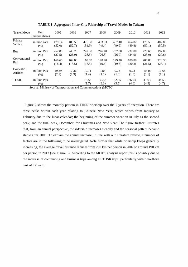
TABLE 1 Aggregated Inter-City Ridership of Travel Modes in Taiwan

Travel Mode Unit

(market share) 2005 2006 2007 2008 2009 2010 2011 2012

Private

Vehicle million cars

(%)

479.14 (52.0)

480.59 (52.7)

475.50 (51.9)

453.93 (49.4)

457.10 (49.9)

464.82 (49.8)

479.55 (50.1)

482.80 (50.5)

Bus million Pax

(%)

252.80 (27.5)

245.20 (26.9)

242.30 (26.5)

246.40 (26.8)

237.80 (26.0)

232.80 (24.9)

220.60 (23.0)

197.05 (20.6)

Conventional

Rail million Pax

(%)

169.60 (18.4)

169.00 (18.5)

169.70 (18.5)

178.70 (19.4)

179.40 (19.6)

189.80 (20.3)

205.83 (21.5)

220.30 (23.1)

Domestic

Airlines million Pax

(%)

19.29 (2.1)

17.36 (1.9)

12.71 (1.4)

9.85 (1.1)

9.23 (1.0)

9.73 (1.0)

10.48 (1.1)

10.68 (1.1)

THSR million Pax

(%) - -

15.56 (1.7)

30.58 (3.3)

32.35 (3.5)

36.94 (4.0)

41.63 (4.3)

44.53 (4.7)

Source: Ministry of Transportation and Communications (MOTC)

Figure 2 shows the monthly pattern in THSR ridership over the 7 years of operation. There are

three peaks within each year relating to Chinese New Year, which varies from January to

February due to the lunar calendar; the beginning of the summer vacation in July as the second

peak; and the final peak, December, for Christmas and New Year. The figure further illustrates

that, from an annual perspective, the ridership increases steadily and the seasonal pattern became

stable after 2008. To explain the annual increase, in line with our literature review, a number of

factors are in the following to be investigated. Note further that while ridership keeps generally

increasing, the average travel distance reduces from 230 km per person in 2007 to around 190 km

per person in 2013 (see Figure 3). According to the MOTC analysis report this is possibly due to

the increase of commuting and business trips among all THSR trips, particularly within northern

part of Taiwan.

9

FIGURE 2 THSR monthly ridership.

FIGURE 3 THSR ridership and average trip distance

As service attributes such as travel speed and fares remain stable over the years, these cannot be

used as explanatory variables. Service frequency varies over the time period but the causality

between demand and supply is not clear. We presume that service frequency will be, at least to a

large degree, an endogenous factor as the operator reacts to increased demand as long as there is

spare capacity. The THSR has reported that the number of services has risen from 1,034 (January

2007) to 4,032 (February 2013) per month. However, this was not a gradual increase but rather

0

500,000

1,000,000

1,500,000

2,000,000

2,500,000

3,000,000

3,500,000

4,000,000

4,500,000

Jan Feb Mar Apr May Jun Jul Aug Sept Oct Nov Dec

Nu

mb

er

of

pas

sen

gers 2013

2012

2011

2010

2009

2008

2007

0

50

100

150

200

250

0

500,000

1,000,000

1,500,000

2,000,000

2,500,000

3,000,000

3,500,000

4,000,000

4,500,000

2007 2008 2009 2010 2011 2012 2013 2014

Average trip

distan

ce (km)N

um

ber

of

pas

sen

gers

(p

pl)

Ridership (ppl) Avg. trip distance (km)

10

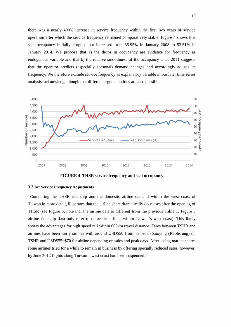
there was a nearly 400% increase in service frequency within the first two years of service

operation after which the service frequency remained comparatively stable. Figure 4 shows that

seat occupancy initially dropped but increased from 35.95% in January 2008 to 53.51% in

January 2014. We propose that a) the drops in occupancy are evidence for frequency as

endogenous variable and that b) the relative smoothness of the occupancy since 2011 suggests

that the operator predicts (especially seasonal) demand changes and accordingly adjusts its

frequency. We therefore exclude service frequency as explanatory variable in our later time series

analysis, acknowledge though that different argumentations are also possible.

FIGURE 4 THSR service frequency and seat occupancy

3.2 Air Service Frequency Adjustments

Comparing the THSR ridership and the domestic airline demand within the west coast of

Taiwan in more detail, illustrates that the airline share dramatically decreases after the opening of

THSR (see Figure 5, note that the airline data is different from the previous Table 1. Figure 5

airline ridership data only refer to domestic airlines within Taiwan’s west coast). This likely

shows the advantages for high speed rail within 600km travel distance. Fares between TSHR and

airlines have been fairly similar with around USD$50 from Taipei to Zuoying (Kaohsiung) on

TSHR and USD$55~$70 for airline depending on sales and peak days. After losing market shares

some airlines tried for a while to remain in business by offering specially reduced sales, however,

by June 2012 flights along Taiwan’s west coast had been suspended.

0

10

20

30

40

50

60

70

80

90

0

500

1,000

1,500

2,000

2,500

3,000

3,500

4,000

4,500

5,000

2007 2008 2009 2010 2011 2012 2013 2014

Seat o

ccup

ancy p

er m

on

th

Nu

mb

er

of

serv

ice

s

Service Frequency Seat Occupancy (%)

11

FIGURE 5 Comparison of THSR and airline (West Coast of Taiwan) monthly ridership.

3.3 (Largely) Exogenous Factors Potentially Affecting THSR Ridership

Besides the above discussed air developments, clearly transport developments for other modes

might have impacted the modal share. For instance the extension or lane widening of the

expressway increased capacities for both private vehicles and buses which could have a negative

impact on rail demand. The expressway network in Taiwan extended from 373 km in 1978 to 989

km in 2009. Guo and Feng (2008) argue that this well connected network (3 north-souths

orientated and 17 east-west orientated expressway networks) has induced 5% car volume each

year in the last 15 years, and forced conventional rail to reduce service frequency on some routes.

Also the fuel price may lead to fare changes for buses, domestic airlines, and directly affects the

travel cost of private vehicles. Whereas in 2012 fuel prices remain relatively stable with a price of

around 1.01 to 1.16 USD per litre, in July 2008 fuel prices reached a peak of 1.16 USD and then

quickly dropped to 0.68 USD at the end of 2008 due to the global financial crisis.

Most studies and previous literature examining gasoline prices have used real gasoline prices

(Lane, 2012). In reality, gasoline prices in Taiwan are supervised by Ministry of Economic

Affairs, but authorized to Chinese Petroleum Corporation (CPC, Taiwan), to determine changes

in prices. The gasoline price varies frequently and unpredictably between weeks. Thus in this

paper, fuel prices was aggregated into monthly averages.

Further, since we are discussing nationwide intercity travel demand, global economic events

such as the 2008 crisis cannot be ignored. Most of the inter-city travel demand generally

decreased in the later half of 2008 and early 2009 (see also 2008 data in Table 1 and Figure 4)

12

except for travel by expressway buses. The reason might be that this service provides the lowest

travel cost among the mode choice option and not capturing much business travel. As a

macroeconomic indicator for this study we therefore collected information on the Gross

Domestic Product (GDP) in Taiwan. GDP data could be obtained as seasonal data from the first

quarter of 2007 (2007Q1) to the fourth quarter of 2012 (2012Q4). Annual comparison shows that

in 2008 and 2011 the GDP declined by 3.26% and 0.02%, while 2007, 2009, 2010, and 2012 the

GDP increased by 2.23%, 3.99%, 2.84% and 1.12% respectively. We note that it might take some

time before the macroeconomic impacts become visible in the demand as suggested by Kyte

(1988) and Lane (2012).

We further note that there is a high correlation between fuel price and GDP (0.794 for Pearson

test), thus in our subsequent analysis in Sections 5 and 6, we use (GDP) / (Fuel price) for a given

month as a measure of “disposable income for petrol”. The expected sign for the impact of this

variable on rail demand should hence be negative, i.e. the more disposable income for petrol, the

less attractive rail is.

As a further economic indicator for effects not captured with the seasonal GDP we consider the

monthly unemployment ratio in Taiwan. The monthly unemployment data could be collected

from the webpage of the Taiwan National Statistics (2013). The ratio varies between 3.78% and

6.13% with a mean of 4.61% within our specified time period.

Besides these economic factors, total population data was collected from the Ministry of the

Interior as a proxy-measurement (Owen and Phillips, 1987; Kyte, 1988; Gwilliam, 2008; Lane,

2012) for THSR market size. We note that the Taiwan west coast holds about 90% of the total

population, thus using nationwide population data appears acceptable. The population shows a

slow but steady increase from 22.87million in January 2007 to 23.33 million in December 2012.

It should be noted that from its prediction, Taiwan will face a population decline after 2018 due

to the low birth ratio (Wang et al., 2009).

As a second related measurement to “market size” as well as economic development, we include

the population’s car ownership ratio. Our data shows that in 2007 there were 29.6 cars per 100

Taiwanese, then ownership declined in 2008 until nearly the end of 2009. Since 2010 the

ownership has been rising again and has reached 30% by the middle of 2011.

For a seasonal demand analysis, holidays should be considered as an important factor (Quddus

et al., 2007) which create additional demand. Reflecting our observations in Figure 2 we

consider Chinese New Year (winter vacation), summer vacation and all three-day consecutive

holidays (Spring breaks, Dragon Boat Festival, Moon Festival, Christmas and New Year Holiday)

as potential sources of high speed rail demand. For Chinese New Year, many will travel to visit

13

families whereas for summer and other holidays significant travel to island and festivals held

across the country is generated.

Finally, in line with our aforementioned discussion that demand adaptation is likely to require

some time and that cyclic effects might encourage more shift of demand after some initial users

have been attracted we include a trend or “adaptation effect” variable which we specify as being

related to the time since service operation and presume to have a positive effect.

14

TABLE 2 Definition, Expected Sign and Descriptive Statistics of Variables

Variables Definition/ Notes Expected sign

in model

Unit Type Minimum Maximum Mean

THSR

THSR Ridership

(Dependent) Total ridership per month

person

Continuous /

Monthly 724,784 4,023,302 2,826,824

Number of

Services High speed rail train services per month

Service

frequency

Continuous /

Monthly 1,034 4,524 3,620

Social

Economic

Factors

Total Population

+ person

Continuous /

Monthly 22,879,132 23,328,602 23,102,882

Unemployment

Ratio

- %

Continuous /

Monthly 3.78 6.13 4.61

GDP Transformed into GDP / Fuel Price as 1

independent variable due to high

correlation

USD /

person

Continuous /

Seasonal 3,823 5,398 4,592

Fuel Price

USD / L Continuous /

Monthly 0.69 1.19 0.98

GDP / Fuel Price Substitution for both explanatory variables,

GDP and Fuel Price

-

Continuous /

Monthly 120.14 196.27 152.15

Airline Airline Ridership

Total ridership along west coast (Taipei-

Taichung, Taipei-Chiayi, Tapei-Tainan,

Taipei-Kaohsiung, Taipei-Pingtung)

person Continuous /

Monthly 0 288,599 33,915

Private Vehicles Car Ownership

Ratio cars per 100 persons

- %

Continuous /

Monthly 29.10 31.00 29.74

Holidays &

Vacations

Chinese New

Year Winter vacation, based on lunar calendar

+

Dummy /

Monthly 0 1 0.31

Summer Vacation Every July / August +

Dummy /

Monthly 0 1 0.37

Consecutive

Holidays

Holiday over 3 days off in a row, e.g.,

Spring Break, Christmas, and New Year

Holiday

+

Dummy /

Monthly 0 1 0.23

Adaptation

effects

Assumed that effects grow larger after the

operation

+

Continuous /

Monthly 1 72 36.5

15

4. SARIMA TIME SERIES MODEL

In order to distinguish seasonal from overall trends, a time-series seasonal autoregressive

integrated moving average (SARIMA) model is used to estimate the demand for THSR 2013

monthly ridership based on data from January 2007 to December 2012. The type of SARIMA

model is usually denoted by SARIMA (p,d,q)(P,D,Q)s model: p and P represent the order of the

non-seasonal and seasonal autoregressive (AR) process; d and D the order of the non-seasonal

and seasonal difference process; q and Q represent the order of non-seasonal and seasonal

moving average (MA) processes. The subscript s denotes the length of seasonality, i.e., in this

model s =12 in case of monthly time series data and due to the annual repetitive character of

some demand, such as new year festivities related journeys.

A fuller description of SARIMA modelling can be found in Andreoni and Postorino (2006).

Examining the autocorrelation function (ACF) and the partial autocorrelation function (PACF)

from time series data we could identify the values of each of these parameters. Based on this

preliminary analysis we suggest to employ a SARIMA model of the order (0,1,2)(0,1,1)12. The

model is given by:

�̂�(𝑡) = 𝜇 + 𝑌(𝑡 − 12) + (𝑌(𝑡 − 1) − 𝑌(𝑡 − 13)) − 𝜃1𝑒(𝑡 − 1) − 𝜃2𝑒(𝑡 − 2)

−Θ𝑒(𝑡 − 12) + 𝜃1Θ𝑒(𝑡 − 13) + 𝜃2Θ𝑒(𝑡 − 14) (1)

Besides the mean μ the model includes three parameters to be estimated. The two non-seasonal

moving average terms θ1 and θ2 as well as the seasonal moving average Θ. The model form hence

suggests that the ridership can be estimated by considering the ridership estimates in the last

month and the ridership one year (season) ago. The three parameters describe the “smoothing

process” due to past outliers and the double exponential smoothing for the non-seasonal part

suggests that there is some underlying non-stationary trend.

Table 3 illustrates the high significance of first and second order moving averages and that the

seasonal moving average is significant at 10% level. The model can thus be used to forecast 2013

monthly ridership and the predicted ridership is compared with observed ridership in Figure 6.

Note that for illustration of the predictive power of the model we only estimate the parameters

with data up to December 2012. The values starting from January 2013 are predicted by our

model. We find a fairly good fit, though the February 2013 peak was not predicted by the model.

This peak can be explained by a non-recurring large event, the Lantern festival, which was held

next to THSR Hsinchu station that month (see also Figure 8).

16

TABLE 3 SARIMA Model Estimation Results for THSR Monthly Ridership

Parameters Coeff. t-statistics p-value

Moving Average MA(1), 𝜃1 0.69 6.30 <0.01

Moving Average MA(2), 𝜃2 -0.55 -4.50 <0.01

Seasonal Moving Average SMA(1), Θ 0.84 1.81 0.08

Differencing: 1 regular and 1 seasonal of length 72

Constant -10439.18 -1.20 0.24

Observation 72

R-square 0.85

Adjusted R-square 0.53

Ljung-Box Q test 0.63

FIGURE 6 Comparison of THSR observed and predicted monthly ridership.

5. TIME SERIES MODEL WITH EXPLANATORY VARIABLES

To further identify the existence of a trend that can be explained with an adaptation effect in this

section, we further use a number of explanatory variables as exogenous factors discussed in

Section 3 and summarised in Table 2. The table also includes the expected sign for each variable.

Our aim is to understand whether there are residual ridership adaptation effects if we control for

other explanatory factors.

The dependent variable remains THSR ridership. To avoid over fitting, we choose for this

analysis a simpler model structure. Log-linear and linear versions of AR(1) and MA(1) models

0

500,000

1,000,000

1,500,000

2,000,000

2,500,000

3,000,000

3,500,000

4,000,000

4,500,000

2007 2008 2009 2010 2011 2012 2013

Nu

mb

er

of

pas

sen

gers

Observed Ridership Predicted Ridership by SARIMA

Model

prediction

starts

17

have been tested. Log-linear MA(1) models are found to provide slightly better model fits.

Therefore, two first-ordered moving average model MA (1) are discussed in the following. The

models are given by:

lnyt=α+βlnXt+θDt+εt (2)

where the error term satisfies:

εt=ρεt-1+ηt (3)

In this model yt is the THSR ridership for month t where we measure months continuously since

operation begin. X is a k * 1 vector of continuous explanatory variables, D is a m * 1 vector of

dummy variables, εt are the white noise or error terms, ρ (-1<ρ<1) is the moving average

coefficient, where η is independent and identically distributed with mean zero and variance σ2.

Finally, βand θrepresent the coefficients of continuous variables X and dummy variables D,

respectively, which are to be estimated.

Results of both models are shown in Table 4 and the explanatory power of both models are

illustrated in Figure 7. Our two models differ in terms of the included explanatory variables.

Model 1 is a minimal model excluding any multi-collinearity problems among the explanatory

variables. Coefficients significant at the 5% level are shown in bold, whereas coefficients

significant at the 10% are indicated in italic.

We find that, as expected, Chinese New Year and summer vacation have a positive effect on

THSR ridership while “consecutive holidays” does not have a significant sign and is excluded

from our model specifications.

GDP / fuel price has the expected negative sign. Further, in our model specification we tested

lag effects of the socio-economic factors. For the GDP/ fuel price factor we find that a lag of one

month provides the best model fit which is in line with Kyte (1988) and Lane (2012) who also

discuss that such lagged responses are reasonable and important behavioural components in

consumer response to changes in marketplace. The lag can be explained by the fact that fuel

prices as well as GDP take time to influence people’s decision.

In model 2 we added the other socio-economic factors such as total population, unemployment

ratio and car ownership. The model results show that population has a significant positive effect

both on lag 0 and lag 1. Unemployment ratio was suggested to have a 3 month lag on THSR

ridership with significant negative effect as expected. Car ownership in this paper was considered

as potential alternative mode choice for travellers. The relationship between THSR and car

ownership is found to be, as expected, negatively significant, suggesting that if one owns a car

18

this has also influence on inter-city travel mode choice. Note that the model fit only slightly

increases by adding the additional variables though the significance of the constant vanishes in

Model 2.

The adaptation effect is included as a continuous variable for months since operation (from

January 2007 to December 2012) in both models. The effect is found to have a strongly

statistically positive sign. We note that the adaptation effect is likely to capture a combination of

various effects. That is, it includes possibly some of the endogenous effects not captured in the

model as well as some of the “information mass effects” discussed in Schmöcker et al (2013). For

example it might take some time before the population gets fully aware of the service quality and

gets convinced it is safe to use. Also businesses trips might have only over time adjusted their

schedules. From personal experience, the first author of this paper knows that since a few years

now, more one-day business trips between Tainan and Taipei are conducted. Whereas before the

introduction of THSR one would arrange for longer, infrequent meetings, nowadays company

executives can conduct morning meetings in Taipei and same day afternoon meetings in Tainan

or Taichung. Thus, one might conclude that the TSHR is slowly changing the “mobility culture”

of private as well as business people of the country.

TABLE 4 Model Estimation Results for Time-series Models

Model: Loglinear with MA(1) Model 1 Model 2

Parameters Lag Coeff. t-statistics Coeff. t-statistics

Total Population 0

190.54 2.81

1

178.06 2.64

Unemployment Ratio 3

-0.65 -4.35

GDP/Fuel Price 1 -0.30 -2.03 -0.31 -2.76

Car Ownership 0

-7.52 -2.99

Chinese New Year 0 0.05 1.82 0.06 2.37

Summer Vacation 0 0.08 2.77 0.04 1.87

Adaptation Effects 0 0.44 28.48 0.51 6.27

Constant

14.82 19.82 -170.63 -0.57

Observation

72 72

R-square

0.96 0.97

Adjusted R-square

0.95 0.96

Moving Average Coeff.

-0.51 -4.63 -0.26 -2.01

Ljung-Box Q test 0.00 0.06

19

FIGURE 7 Comparison of observed and predicted monthly ridership (Models 1 & 2).

6. APPLICATION TO STATION DEMAND

To confirm our above findings and to understand whether parameter estimates vary significantly

depending on the location, in this section we use the same methodology as above for the ridership

of two specific stations. We choose for this Taipei and Hsinchu. Taipei is the capital and largest

city of Taiwan with a population of around 6.6 million at the end of 2012. The high speed rail

station will be used by all kind of travellers including business travellers as well as local and

some foreign tourists. We contrast this with Hsinchu, a city known for its world leading IT

industries and located 30 minutes away from Taipei by high speed rail, with a population of

nearly 0.95 million. The station locations and access possibilities also differ in the two cities.

Taipei has a well-connected public transport network and THSR station is located right in the

middle of downtown. Hsinchu station is located about 9 km outside of its CBD but close to the IT

industry cluster, emphasising the primary importance of this station for business travel. Figure 8

illustrates the ridership development for both stations in terms of number of passengers at the

respective stations. Taipei has the largest ridership among all the HSR stations and illustrates a

growth pattern with fairly significant monthly variations. In contrast the growth in Hsinchu is

smoother (except for the February 2013 peak mentioned above) and at a much lower level.

To replicate the above MA(1) model specified with equations (2) and (3) we use the same

variables that were found significant in Table 4. Only for population, unemployment and car

0

500,000

1,000,000

1,500,000

2,000,000

2,500,000

3,000,000

3,500,000

4,000,000

4,500,000

2007 2008 2009 2010 2011 2012

Nu

mb

er

of

pas

sen

gers

Observed Ridership Predicted fit by MA(1) Model_1 Predicted fit by MA(1) Model_2

20

ownership ratio the national data are replaced with regional data (Table 5). Note further that due

to underground construction in Taipei, THSR was opened two month later compared to other

stations, so that for Hsinchu we have 72 data points but only 70 data points for Taipei (Table 5).

TABLE 5 Descriptive Statistics of Taipei and Hsinchu Data

Variables Taipei Hsinchu

Min. Max. Mean Min. Max. Mean

THSR Ridership 516,115 2,299,498 1,163,122 82,539 764,880 469,034

Social

Economic

Factors

Total Population 6,401,666 6,612,531 6,493,899 883,482 949,064 918,426

Unemployment

Ratio 3.70 5.80 4.52 3.72 5.86 4.50

GDP / Fuel Price 120.14 196.26 152.32 120.14 196.26 152.32

Private

Vehicles

Car Ownership

Ratio 202.62 252.59 239.88 259.70 306.46 288.91

Holidays

&

Vacations

Chinese New Year 0 1 0.31 0 1 0.31

Summer Vacation 0 1 0.37 0 1 0.37

Adaptation effects 1 70 35.5 1 72 36.5

Data taken from: …

FIGURE 8 Number of passengers at Taipei and Hsinchu stations

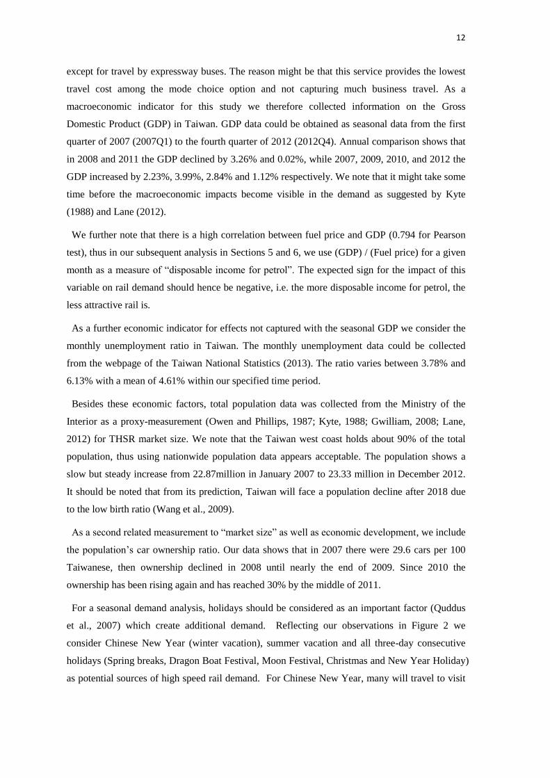
Table 6 shows our results for both cities. We find that population has the expected positive

impact on Taipei ridership but we do not find this for Hsinchu. Both cities show significant

negative parameters for unemployment, and significant positive ones for summer vacation and

the adaptation effects, consistent with our model in section 5. We further find that GDP/Fuel

price is only weakly significant for Taipei ridership, possibly because of the generally higher

prices in Taiwan leading to less price sensitivity and/or due to a lower proportion of business

0

500,000

1,000,000

1,500,000

2,000,000

2,500,000

2007 2008 2009 2010 2011 2012 2013

Nu

mb

er

of

pas

sen

gers

Taipei

Hsinchu

21

trips among Taipei demand. The second argument is further supported by the fact that GDP/Fuel

price is highly significant in Hsinchu with a parameter that is larger than for the aggregate model

in Table 4.

For similar reasons Chinese New Year (generally considered as back home trips) might not be

significant for Taipei, that is the proportion of additional “return home” trips are not significant

compared to the overall demand. Instead, in Hsinchu we find a negative parameter for Chinese

New Year due to the larger proportion of business trips which are reduced during this holiday

period. The adaptation effect is strongly significant in both cities, in particular for Hsinchu with a

parameter larger than the one observed for the aggregate data. We suggest that this might be due

to the above discussed change in business patterns and adaptation of commuters who over time

start using more often the high speed rail especially for trips from/to Taipei. In support of this

argument we remind that Figure 3 illustrates that average trip distance of travellers has been

reducing, which suggests more usage of high speed rail for short distance commuting trip.

TABLE 6 Model Estimation Results for Taipei and Hsinchu

Model: Loglinear with MA(1) Taipei Hsinchu

Parameters lag Coeff. t-statistics Coeff. t-statistics

Total Population 0 529.76 2.14 -82.07 -1.23

1 551.10 2.19 -70.69 -1.07

Unemployment Ratio 3 -0.48 -4.95 -0.44 -3.15

GDP/Fuel Price 1 -0.21 -1.80 -0.39 -3.13

Car Ownership 0 0.31 1.24 0.09 0.37

Chinese New Year 0 0.01 0.39 -0.05 -2.09

Summer Vacation 0 0.06 2.73 0.07 2.84

Adaptation Effects 0 0.61 12.45 0.95 13.66

Constant

346.89 4.54 168.29 4.91

Observation

70 72

R-square

0.95 0.98

Adjusted R-square

0.94 0.97

Moving Average Coeff.

-0.21 -1.51 -0.52 -4.44

Ljung-Box Q test 0.11 0.00

7. CONCLUSIONS AND FUTURE RESEARCH

In this paper we reviewed demand uptake of the newly introduced Taiwan High Speed Rail

since 2007. We discuss its effect on competing modes such as air and highway traffic showing

that the new system has slowly driven domestic air transport out of market. This might be an

22

encouraging message for other countries aiming to introduce more sustainable rail transport for

medium long distance travel. However, one also has to remember the specific geography of

Taiwan, where a single high speed rail line can capture most of the air demand.

We present two types of time series modelling and two specific scale of data to test our model

performance. Our fitted SARIMA model appears suitable for demand forecasting whereas our

simpler MA(1) models help us understanding the role of specific exogenous factors for aggregate

as well as station specific demand.

For aggregate forecasting we find that total population, GDP, unemployment and fuel prices as

well as seasonal effects are significant determinants of demand, all with the expected sign. This

suggests that to estimate demand precisely one needs to take into account a mixture of long-term

predictable factors (such as population growth) as well as short term fluctuating factors (such as

fuel price). For station specific demand socio-demographics, GDP, fuel price, and car ownership

may not always be significant. Rather it is important to understand the composition of the trip

purposes of the travellers as our analysis of demand patterns for Hsinchu and Taipei suggests.

The focus of our study has been on the adaptation effect. We estimate this with continuous log-

linear dummy variable representing the duration since operation. We find this factor highly

significant for both aggregate as well as local demand. Even after seven years of operation it is

not obvious when and whether equilibrium might be reached, which has possibly implications for

demand modelling of any kind of new transport system such as electric cars or shared car

schemes. Policy makers should be careful in over predicting the short term demand a new scheme

might generate. We argue that this is possibly due to various types of “adaptation effects”

including general population perception of the new scheme and possibly “information spread”.

Our analysis of Hsinchu versus Taipei ridership patterns further tentatively suggests that

adaptation effect might be stronger for business than for private travel. We acknowledge though

that further work is needed to confirm this by disentangling the different factors combined in the

adaptation effect. This is though not possible with the data currently available. Instead we suggest

one might need to look into individual personal trip patterns, and in addition to conduct a more

qualitative study interviewing business as well as private travellers on when and why they started

using the high speed rail service.

In discussions on the cost-effectiveness of potential high speed rail projects often expected

ridership data are published. We propose that adaptation effects to new systems might take a

significant time and initial low ridership might not be a sign of “wrong estimates”. Demand

estimation for new systems that potentially significantly change the mobility patterns of a wider

region might have to be treated very differently than demand estimation for system extensions.

For example, data from German rail suggest that for recently built or upgraded high speed routes

23

it takes around three to four years for demand to stabilise. Also data from the recently opened

high speed rail extension in Kyushu, Japan, suggest that total ridership appears to stabilise fast. In

both cases the population will have been already used to the high speed rail concept and fairly

easily adapt their behaviour.

Clearly the present study leaves ample room for further work besides the already mentioned

issues. One extension of the present study would be to continue with a detailed comparison of

ridership between all eight THSR stations. This could be used to better understand the role of

local and regional factors as well the importance of station location and access possibilities.

Connected with this, as our Figure 1 shows, there appears to be a general shift away from bus to

rail in Taiwan. Though we believe in some sense non-high speed rail also profits from this,

further analysis should clarify the interdependencies between demands for these modes. In

particular, it appears worthwhile to investigate in how for THSR rail profits or losses by

improvements to other rail lines.

REFERENCES

Abrate, G., M. Piacenza, and D. Vannoni. The impact of Integrated Tariff Systems on public

transport demand: Evidence from Italy. Regional Science and urban Economics, Vol. 39,

2009, pp. 120-127.

Ahlfeldt, G.M., and A. Feddersen. From periphery to core: economic adjustments to high speed

rail. London School of Economics & University of Hamburg, 2010.

Andersson, D.E., O.F. Shyr, and J. Fu. Does high-speed rail accessibility influence residential

property prices? Hedonic estimates from southern Taiwan. Journal of Transport Geography,

Vol, 18, 2010, pp. 166-174.

Andreoni, A., and M.N. Postorino. A multivariate ARIMA model to forecast air transport

demand. Association for European Transport, 2006.

Bass, P., P. Donoso, and M. Munizaga. A model to assess public transport demand stability.

Transportation Research Part A, Vol. 45, 2011, pp. 755-764.

Belgiawan, P.F., J-D. Schmöcker, and S. Fujii. Explaining the Desire to Own a Car among

Indonesian Students. In Proceedings of the 32nd Japan Society of Traffic Engineers

Conference. CD ROM. Japan Society of Traffic Engineers, Tokyo, 2012, pp.259-266.

Chao, C.W., O.F. Shyr, C.H. Chao, and L. Tsai. What drives college-age generation Y’s

perceived value on high speed rail. African Journal of Business Management, Vol. 6, No. 43,

2012, pp. 10786-10790.

Cheng, Y.H. High-speed rail in Taiwan: New experience and issues for future development.

Transport Policy, Vol. 17, 2010, pp. 51-63.

24

Chen, Z. H. Who Ride the High Speed Rail in the United States: The Acela Express Case Study.

2010 Joint Rail Conference, April 27-29, 2010, Urbana, Illinois, USA. Available at SSRN:

http://ssrn.com/abstract=1729816

DeMaio, P. Bike-sharing: History, impacts, model of provision, and future. Journal of Public

Transportation, Vol. 12, No. 4, 2009, pp. 41-56.

Fishman, E., S. Washington, and N. Haworth. Bike share: A synthesis of the literature. Transport

Reviews: A Transnational Transdisciplinary Journal. DOI:10.1080/01441647.2013.775612,

2013.

FitzRoy, F., and I. Smith. Public transport demand in Freiburg: why did patronage double in a

decade? Transport Policy, Vol. 5, 1998, pp. 163-173.

Fu, X., T.H. Oum, and J. Yan. An analysis of travel demand in Japan’s intercity market. Journal

of Transport Economics and Policy, Vol. 48, No.1, 2014, pp. 97-113.

Guo F.Y., and H.S. Feng. Establishing Public Transport Service Network by taking THSR as

Transfer Nodes, (in Chinese), Taiwan Economic Forum, Council for Economic Planning &

Development, Department of Urban and Housing Development, Executive Yuan, 2009.

Gwilliam, K. A review of issues in transit economics. Research in Transportation Economics,

Vol. 23, 2008, pp. 4-22.

Ito, H., and D. Lee. Assessing the impact of the September 11 terrorist attacks on U.S. airline

demand. Journal of Economics & Business, Vol. 57, 2005, pp. 75-95.

KMLIT. Korean Ministry of Land, Infrastructure and Transport. Report on AREX Service

Demand. Published in 2009. Available from < http://www.ppip.or.kr/> [In Korean; accessed

October 2013].

Kyte, M., J. Stoner, and J. Cryer. A time-series analysis of public transit ridership in Portland,

Oregon, 1971-1982. Transportation Research-A, Vol. 22A, No. 5, 1988, pp.345-359.

Lane, B.W. A time-series analysis of gasoline prices and public transportation in US metropolitan

areas. Journal of Transport Geography, Vol. 22, 2012, pp. 221-235.

Lee, S.S., and M.L. Senior. Do light rail services discourage car ownership and use? Evidence

from Census data for four English cities. Journal of Transport Geography, Vol. 29, 2013, pp.

11-13.

Lieven, T., S. Muhlmeier, S. Henkel, and J.F. Waller. Who will buy electric cars? An empirical

study in Germany. Transportation Research Part D, Vol. 16, 2011, pp.236-243.

Link, C., U. Raich, G. Sammer, and J. Stark. Modeling demand for electric cars – a methodical

approach. Procedia – Social and Behavioral Sciences, Vol. 48, 2012, pp.1958-1970.

Mohring, H. Optimization and scale economics in urban bus transportation. The American

Economic Review, Vol. 62, No. 4, 1972, pp. 591-604.

Owen, A.D., and G.D.A. Phillips. The characteristics of railway passenger demand: An

econometric investigation. Journal of Transport Economics and Policy, Vol. 21, No. 3, 1987,

pp. 231-253.

Quddus, M.A., M.G.H. Bell, J-D. Schmöcker, and A. Fonzone. The impact of the congestion

charge on the retail business in London: An econometric analysis. Transport Policy, Vol. 14,

2007, pp. 433-444.

25

Republic of China National Statistics, 2013. National Statistics. Available from

<http://ebas1.ebas.gov.tw/pxweb/Dialog/NI.asp>. [Accessed July 15, 2013].

Schmöcker, J.D., Hatori, T., and Walting, D. Dynamic process model of mass effects on travel

demand. Transportation, Vol. 41, No. 2, 2014, pp.279-304.

Su, C-W., C-W., Chang, Y-C., Lu, and J-R. Liu. A Study on Selecting a Feasible Mode for

Seamlessly Transferring between HSR and TR Stations, (in Chinese), ISBN 978-986-03-

3263-6. Ministry of Transportation and Communications, 2012.

Taiwan High Speed Rail (THSR), 2012. Annual Report homepage. Available from

<http://www.thsrc.com.tw/en/about/ab_stock.asp#AnnualReport>, [Accessed July 06, 2013].

Wang, L., Lo, Y.M., Fan, S.C., and W.T. Chao. Analysis of Population Projections for Taiwan

Area: 2008 to 2056, (in Chinese), Taiwan Economic Forum, Council for Economic Planning

& Development, Department of Manpower Planning, Executive Yuan, 2009.