Demagnetisation in Crossed

Fields

Archie Campbell, Mehdi Bagdhadi, Anup Patel, Difan Zhou,

K.Y.Huang Tim Coombs

1) Mikitic Brandt Theory

2) Numerical Calculations

3) Comparison with Experiments

Materials: YBCO pucks and YBCO tapes.

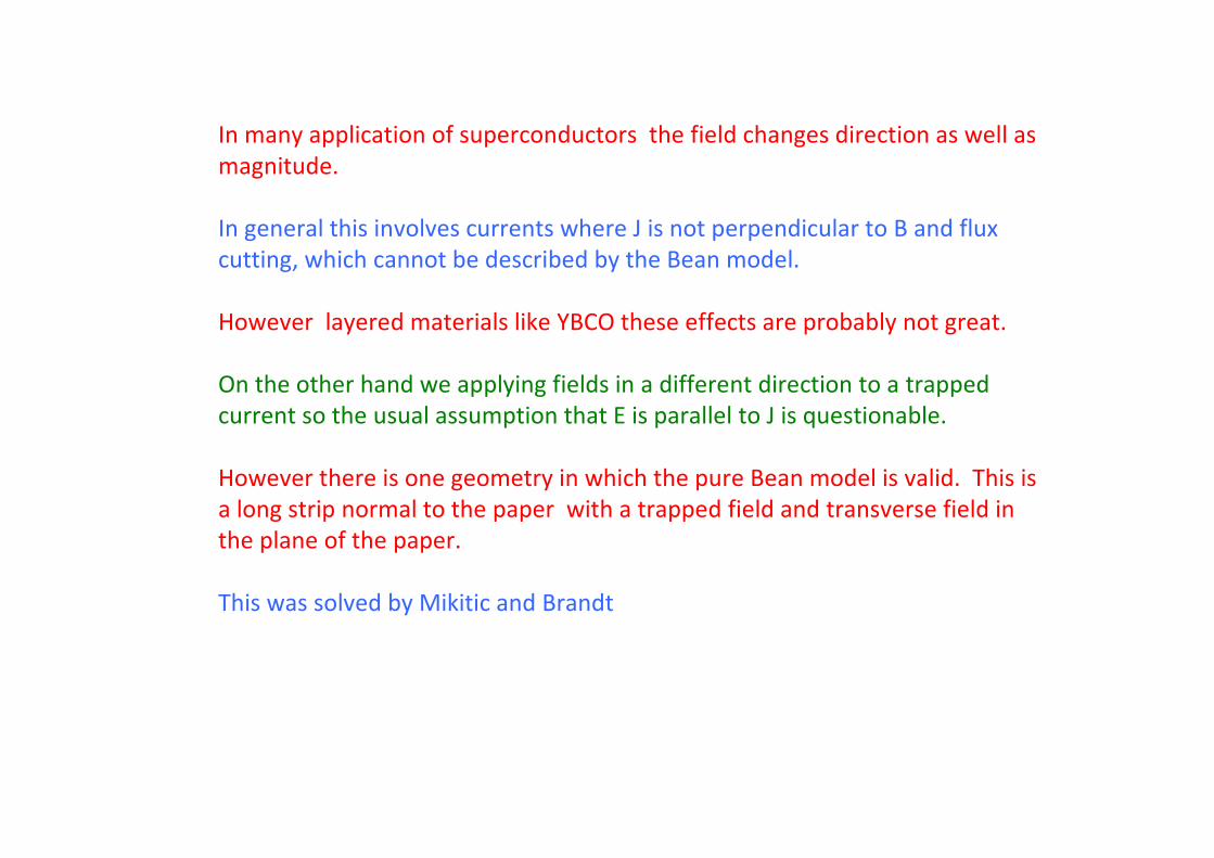
In many application of superconductors the field changes direction as well as

magnitude.

In general this involves currents where J is not perpendicular to B and flux

cutting, which cannot be described by the Bean model.

However layered materials like YBCO these effects are probably not great.

On the other hand we applying fields in a different direction to a trapped

current so the usual assumption that E is parallel to J is questionable.

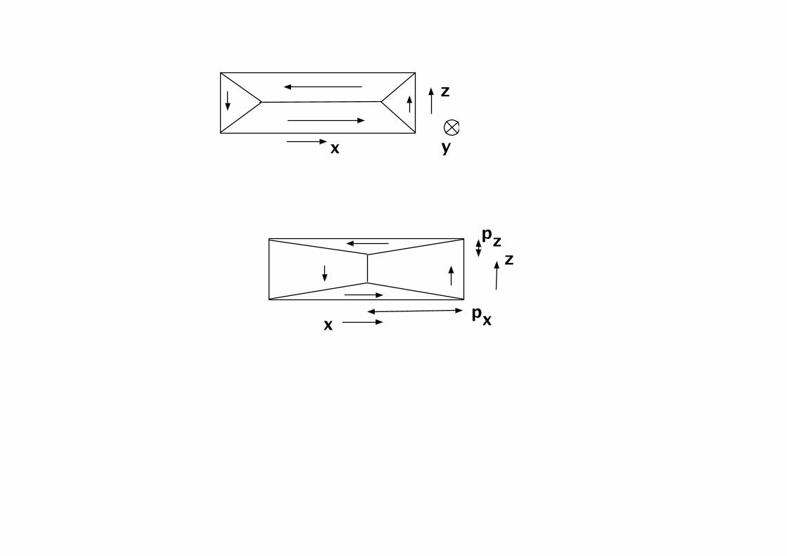
However there is one geometry in which the pure Bean model is valid. This is

a long strip normal to the paper with a trapped field and transverse field in

the plane of the paper.

This was solved by Mikitic and Brandt

N. Sakamoto, F. Irie, and K. Yamafuji, J. Phys. Soc. Jpn. 41, 32 (1976).

At I=Ic Bp(I)=0

At I=0 Bp=Bp(0)=μojcd

The Dynamic Resistance

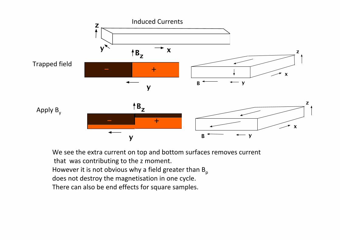
Trapped field

Apply By

Induced Currents

We see the extra current on top and bottom surfaces removes current

that was contributing to the z moment.

However it is not obvious why a field greater than Bp

does not destroy the magnetisation in one cycle.

There can also be end effects for square samples.

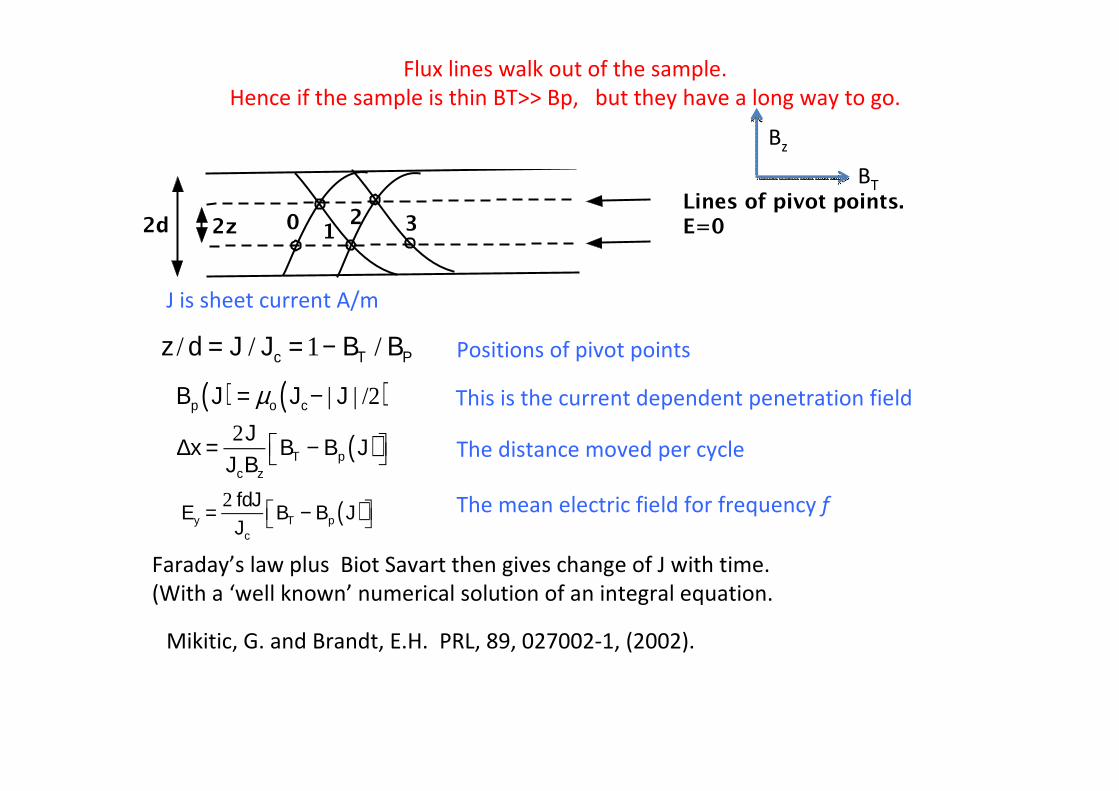
Flux lines walk out of the sample.

Hence if the sample is thin BT>> Bp, but they have a long way to go.

z / d = J / Jc = 1− BT / BP

J is sheet current A/m

∆x = 2JJcBz

BT − Bp J( )

Bp J( ) = µo Jc− | J | /2( )

Ey = 2 fdJJc

BT − Bp J( )

Faraday’s law plus Biot Savart then gives change of J with time.

(With a ‘well known’ numerical solution of an integral equation.

Mikitic, G. and Brandt, E.H. PRL, 89, 027002-1, (2002).

This is the current dependent penetration field

Positions of pivot points

The distance moved per cycle

The mean electric field for frequency f

BT

Bz

If BT<Bp Msat=Mo(1-BT/Bp)

w=width, d thickness

no=fto=w/4d cycles M saturates after

about w/d cycles.

For a 1μ thick YBCO tape this is 10000

cycles.

However Bp is only about 16mT so this is

not very useful for tapes.

However this is the important regime for

bulks.

If BT>Bp at large times M decays

exponentially with a time constant, in cycles

For tape with Ic=300A , width 12mm YBCO thickness 1μ Jc=250A/cm Bp=15.7 mT

At BT=300mT no=175 cycles

It is important to realise that we cannot model the tape by increasing d

and reducing jc in proportion to give the same Bp.

However for thin samples and large BT no=0.25(w/d)(Bp/BT)

Notice that although Mikitic and Brandt asssume a large normal field, the result does not

contain it. The decay time is independent of a uniform applied field.

no =wBp

2πd(0.64) BT − Bp( )μ

16 tapes, 12 mm sq

M. Baghdadi1,a), H. S. Ruiz1 and T. A. Coombs1

Appl. Phys. Lett. 104, 232602 (2014); http://dx.doi.org/10.1063/1.4879263

Mikitic Theory no=175 Cycles

At 300 mT no=1000 cycles, 6x theory

Decay in Stacked Tapes Showed Surprisingly Slow Decay

Trapped field BT=0 Plus half cycle BT=300 mT

Bt=-300 mT After 6 cycles

Real Shape

20mm wide 1mm thick

YBCO puck.

Large penetration.

BT=5Bp

Current patterns are

as expected. Most

of the Mz has

disappeared.

To investigate the validity of the theory a number of simulations were made on a 2cmx1mm

bulk using FlexPDE.

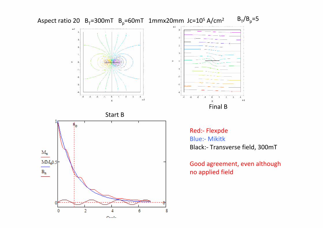
Aspect ratio 20 BT=300mT Bp=60mT 1mmx20mm Jc=105 A/cm2

Red:- Flexpde

Blue:- Mikitk

Black:- Transverse field, 300mT

Good agreement, even although

no applied field

BT/Bp=5

Start B

Final B

Low BT .8xBp,, expect saturation of M

Trapped Field 50 mT -50mT

30 Cycles30 cycles 260 cycles

Still

Trapped

Field

Much Less

Trapped

Field

Red Flexpde

Blue Mikitic

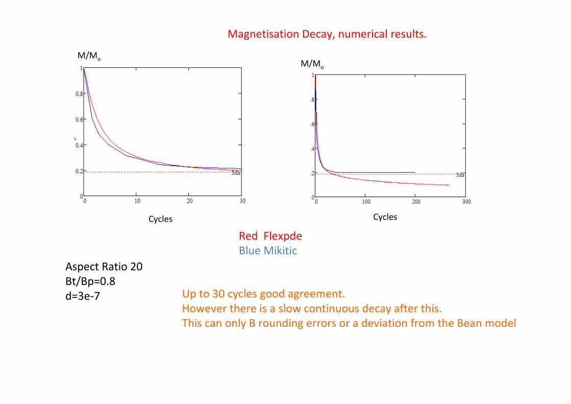
Magnetisation Decay, numerical results.

Aspect Ratio 20

Bt/Bp=0.8

d=3e-7

Cycles Cycles

M/MoM/Mo

Up to 30 cycles good agreement.

However there is a slow continuous decay after this.

This can only B rounding errors or a deviation from the Bean model

R. A. Doyle and A. M. Campbell and R. E. Somekh

PRL 71, 4242-4244, 1993

The flux movement is small in thin layers and

if in linear regime could explain long decay times.

In atomically thin layers there is no space for the critical state so there would be no decay.

However intermediate values give a long term decay.

The A Formulation Used

Force Displacement Curve for Flux Lines Experiment, AC V-I Characteristic

We solve the force balance equation

The parameter ‘d’ defines how close to the true critical state we are.

d=0 is Bean model. Large d gives a linear London equation.

Cycles Cycles

M/Mo

M/Mo

Magnet Decay. Larger Reversible Movement

Black Mikitic (Bean Model)

Red d=3. 10-7

Blue d=10-5

Increasing d reversible movement decreases

decay for up to 30 cycles.

However it increases the long term decay.

For a minor hysteresis loop we impose the same gradient at the start of each sector.

We also impose the condition that it saturates at plus or minus BJc as appropriate.

In general minor hysteresis loops do not close.

The only closed Rayleigh loops are symmetric about zero force.

Hence all hysteretic systems must decay to equilibrium after a sufficient number of cycles.

(e.g. Stress and Permanent Magnetisation).

Minor Hysteresis Loops

Initial flux displacement plus two minor loops Many Loops

Force

Displacement

Force

Displacement

Bulk Experiment on Puck, (Central Trapped Field)

8mm x16

Bp .7

Bt .17

BT/Bp=0.287

We expect saturatation

Red is experiment, Blue FlexPDE

The experimental decay is much

slower than than the simulation.

Could be end effects, enhanced by anisotropy.

The Mikitic theory is only for a single sheet. Since an external field does not affect the

decay time we might expect the tapes to behave independently.

Mehdi Bagdhadi has done a simulation for up to eight decoupled layers,

each 20mm wide by 1mm thick.

He found a large effect.

(These are graphs of integrated Bz across the face using Comsol and the H formulation)

How does a stack behave?

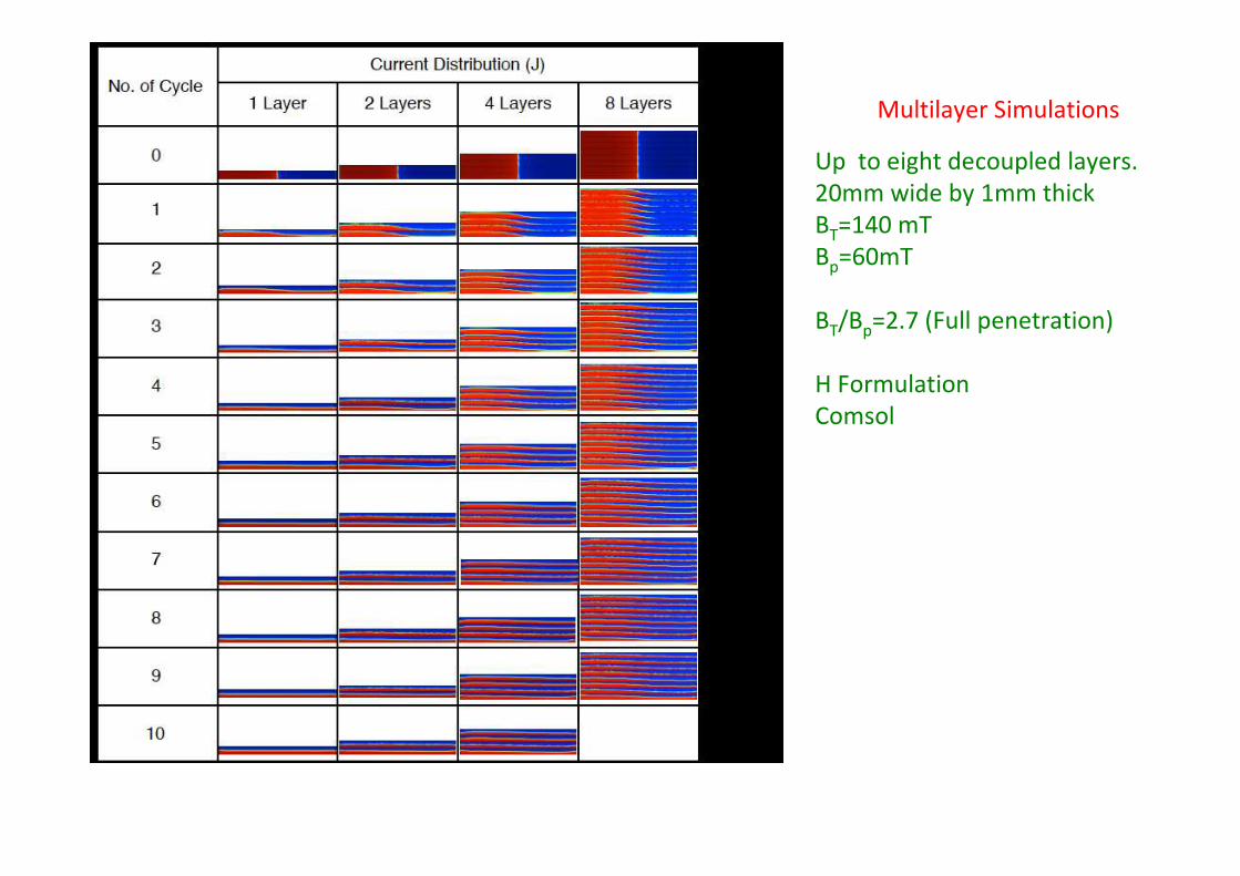
Up to eight decoupled layers.

20mm wide by 1mm thick

BT=140 mT

Bp=60mT

BT/Bp=2.7 (Full penetration)

H Formulation

Comsol

Multilayer Simulations

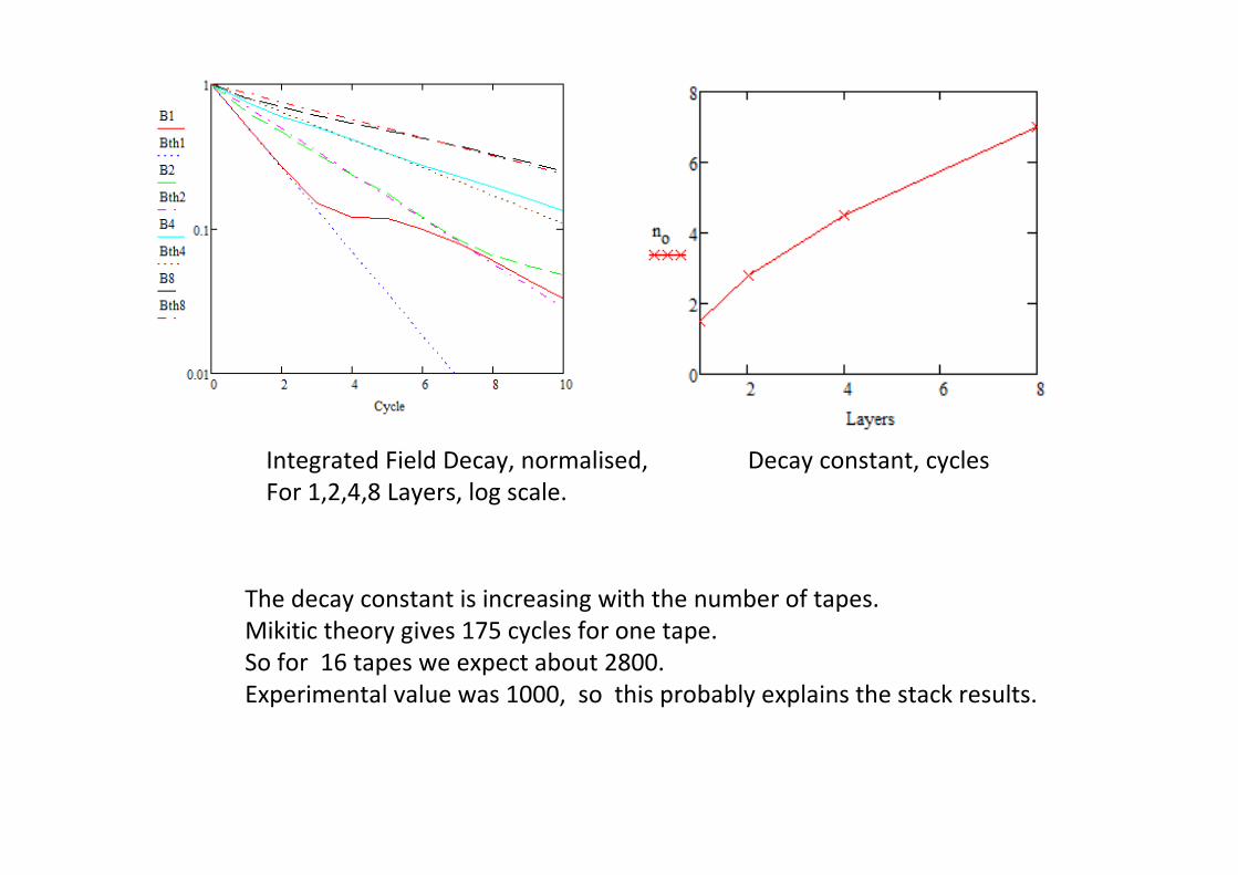
Integrated Field Decay, normalised,

For 1,2,4,8 Layers, log scale.

Decay constant, cycles

The decay constant is increasing with the number of tapes.

Mikitic theory gives 175 cycles for one tape.

So for 16 tapes we expect about 2800.

Experimental value was 1000, so this probably explains the stack results.

Cycles

B/Bo B/Bo

Cycles

Bath group results on YBCO tapes.

Min Zhou, Weijia Yuan

300mT 0t peak, equivalent to 150mT, large cross field

Blue one tape, red three.

Again decay time lengthens with number of tapes.

However the very sharp drop followed by a faster decay than

theory is hard to fit with other experiemnts,

Min 1 and three stack slop 40 cycles

Conclusions

For samples which can be modelled the Miktic Brandt theory works well.

However for large numbers of cycles the magnetisation continues to drop slowly

This could be explained by reversible flux line motion.

This effect can also cause long decay times in very thin samples.

Tapes are too thin to model but stacks of thicker samples show

the decay time increases with the number of layers.

This can explain the slow decay time of YBCO tape stacks.

Experiments on bulk samples show much longer delay times than simulations.

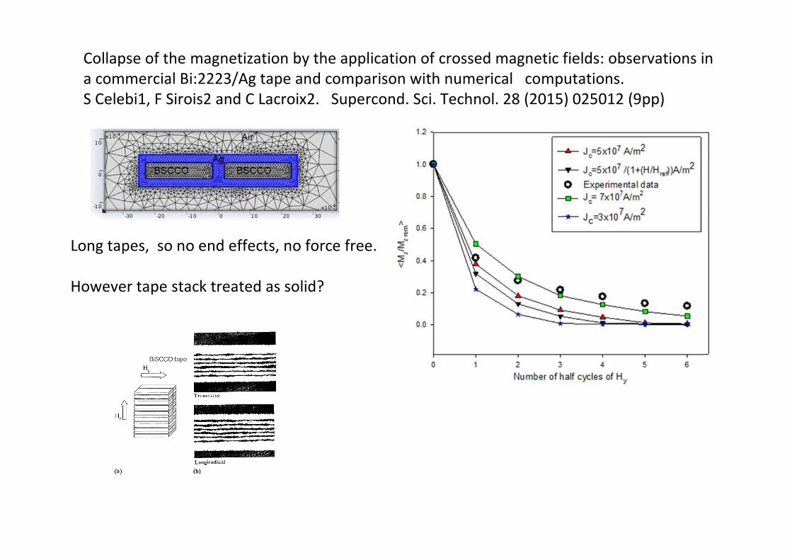
Collapse of the magnetization by the application of crossed magnetic fields: observations in

a commercial Bi:2223/Ag tape and comparison with numerical computations.

S Celebi1, F Sirois2 and C Lacroix2. Supercond. Sci. Technol. 28 (2015) 025012 (9pp)

Long tapes, so no end effects, no force free.

However tape stack treated as solid?

H formulation n value

140 mT