delta function pairs - dspguide.com

209

CHAPTER

11Fourier Transform Pairs

For every time domain waveform there is a corresponding frequency domain waveform, and viceversa. For example, a rectangular pulse in the time domain coincides with a sinc function [i.e.,sin(x)/x] in the frequency domain. Duality provides that the reverse is also true; a rectangularpulse in the frequency domain matches a sinc function in the time domain. Waveforms thatcorrespond to each other in this manner are called Fourier transform pairs. Several commonpairs are presented in this chapter.

Delta Function Pairs

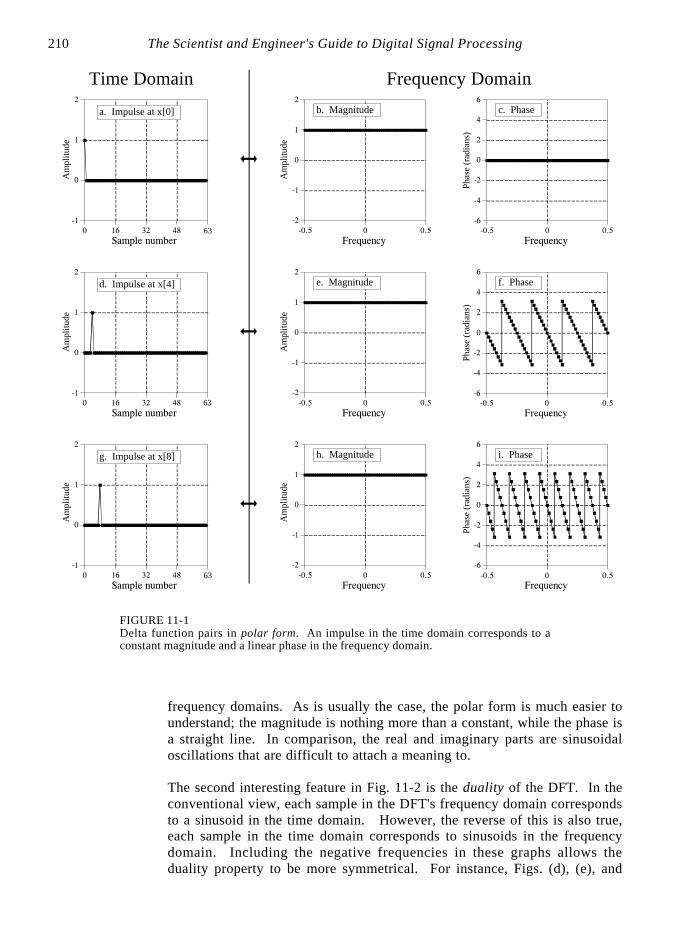
For discrete signals, the delta function is a simple waveform, and has anequally simple Fourier transform pair. Figure 11-1a shows a delta function inthe time domain, with its frequency spectrum in (b) and (c). The magnitudeis a constant value, while the phase is entirely zero. As discussed in the lastchapter, this can be understood by using the expansion/compression property.When the time domain is compressed until it becomes an impulse, the frequencydomain is expanded until it becomes a constant value.

In (d) and (g), the time domain waveform is shifted four and eight samples tothe right, respectively. As expected from the properties in the last chapter,shifting the time domain waveform does not affect the magnitude, but adds alinear component to the phase. The phase signals in this figure have not beenunwrapped, and thus extend only from -B to B. Also notice that the horizontalaxes in the frequency domain run from -0.5 to 0.5. That is, they show thenegative frequencies in the spectrum, as well as the positive ones. Thenegative frequencies are redundant information, but they are often included inDSP graphs and you should become accustomed to seeing them.

Figure 11-2 presents the same information as Fig. 11-1, but with thefrequency domain in rectangular form. There are two lessons to be learnedhere. First, compare the polar and rectangular representations of the

The Scientist and Engineer's Guide to Digital Signal Processing210

Sample number0 16 32 48 64

-1

0

1

2

63

d. Impulse at x[4]


-1

0

1

2

63

a. Impulse at x[0]

Frequency-0.5 0 0.5

-2

-1

0

1

2e. Magnitude

Frequency-0.5 0 0.5

-6

-4

-2

0

2

4

6f. Phase

Frequency-0.5 0 0.5

-2

-1

0

1

2h. Magnitude

Frequency-0.5 0 0.5

-6

-4

-2

0

2

4

6i. Phase

Frequency-0.5 0 0.5

-2

-1

0

1

2b. Magnitude

Frequency-0.5 0 0.5

-6

-4

-2

0

2

4

6c. Phase


-1

0

1

2

63

g. Impulse at x[8]

Frequency DomainTime Domain

Am

plitu

de

Phas

e (r

adia

ns)

Am

plitu

de

Am

plitu

de

Phas

e (r

adia

ns)

Am

plitu

de

Am

plitu

de

Phas

e (r

adia

ns)

Am

plitu

de

FIGURE 11-1Delta function pairs in polar form. An impulse in the time domain corresponds to aconstant magnitude and a linear phase in the frequency domain.

frequency domains. As is usually the case, the polar form is much easier tounderstand; the magnitude is nothing more than a constant, while the phase isa straight line. In comparison, the real and imaginary parts are sinusoidaloscillations that are difficult to attach a meaning to.

The second interesting feature in Fig. 11-2 is the duality of the DFT. In theconventional view, each sample in the DFT's frequency domain correspondsto a sinusoid in the time domain. However, the reverse of this is also true,each sample in the time domain corresponds to sinusoids in the frequencydomain. Including the negative frequencies in these graphs allows theduality property to be more symmetrical. For instance, Figs. (d), (e), and

Chapter 11- Fourier Transform Pairs 211


-1

0

1

2

63

d. Impulse at x[4]


-1

0

1

2

63

a. Impulse at x[0]

Frequency-0.5 0 0.5

-2

-1

0

1

2e. Real Part

Frequency-0.5 0 0.5

-2

-1

0

1

2f. Imaginary part

Frequency-0.5 0 0.5

-2

-1

0

1

2h. Real Part

Frequency-0.5 0 0.5

-2

-1

0

1

2i. Imaginary part

Frequency-0.5 0 0.5

-2

-1

0

1

2b. Real Part

Frequency-0.5 0 0.5

-2

-1

0

1

2c. Imaginary part


-1

0

1

2

63

g. Impulse at x[8]


Am

plitu

de

Am

plitu

de

Am

plitu

de

Am

plitu

de

Am

plitu

de

Am

plitu

de

Am

plitu

de

Am

plitu

de

Am

plitu

de

FIGURE 11-2Delta function pairs in rectangular form. Each sample in the time domain results in a cosine wave in the real part,and a negative sine wave in the imaginary part of the frequency domain.

(f) show that an impulse at sample number four in the time domain results infour cycles of a cosine wave in the real part of the frequency spectrum, andfour cycles of a negative sine wave in the imaginary part. As you recall, animpulse at sample number four in the real part of the frequency spectrumresults in four cycles of a cosine wave in the time domain. Likewise, animpulse at sample number four in the imaginary part of the frequency spectrumresults in four cycles of a negative sine wave being added to the time domainwave.

As mentioned in Chapter 8, this can be used as another way to calculate theDFT (besides correlating the time domain with sinusoids). Each sample in thetime domain results in a cosine wave being added to the real part of the


EQUATION 11-1DFT spectrum of a rectangular pulse. In thisequation, N is the number of points in thetime domain signal, all of which have a valueof zero, except M adjacent points that have avalue of one. The frequency spectrum iscontained in , where k runs from 0 toX[k]N/2. To avoid the division by zero, use

. The sine function uses radians,X[0] ' Mnot degrees. This equation takes intoaccount that the signal is aliased.

Mag X [ k] ' /000sin(BkM /N )

sin(Bk /N )/000

frequency domain, and a negative sine wave being added to the imaginary part.The amplitude of each sinusoid is given by the amplitude of the time domainsample. The frequency of each sinusoid is provided by the sample number ofthe time domain point. The algorithm involves: (1) stepping through each timedomain sample, (2) calculating the sine and cosine waves that correspond toeach sample, and (3) adding up all of the contributing sinusoids. The resultingprogram is nearly identical to the correlation method (Table 8-2), except thatthe outer and inner loops are exchanged.

The Sinc Function

Figure 11-4 illustrates a common transform pair: the rectangular pulse and thesinc function (pronounced “sink”). The sinc function is defined as:

, however, it is common to see the vague statement: "thesinc(a) ' sin(Ba)/ (Ba)sinc function is of the general form: ." In other words, the sinc is a sinesin(x)/xwave that decays in amplitude as 1/x . In (a), the rectangular pulse issymmetrically centered on sample zero, making one-half of the pulse on theright of the graph and the other one-half on the left. This appears to the DFTas a single pulse because of the time domain periodicity. The DFT of thissignal is shown in (b) and (c), with the unwrapped version in (d) and (e). First look at the unwrapped spectrum, (d) and (e). The unwrappedmagnitude is an oscillation that decreases in amplitude with increasingfrequency. The phase is composed of all zeros, as you should expect fora time domain signal that is symmetrical around sample number zero. Weare using the term unwrapped magnitude to indicate that it can have bothpositive and negative values. By definition, the magnitude must always bepositive. This is shown in (b) and (c) where the magnitude is made allpositive by introducing a phase shift of B at all frequencies where theunwrapped magnitude is negative in (d).

In (f), the signal is shifted so that it appears as one contiguous pulse, but is nolonger centered on sample number zero. While this doesn't change themagnitude of the frequency domain, it does add a linear component to thephase, making it a jumbled mess. What does the frequency spectrum look likeas real and imaginary parts ? Too confusing to even worry about.

An N point time domain signal that contains a unity amplitude rectangular pulseM points wide, has a DFT frequency spectrum given by:


Frequency0 0.1 0.2 0.3 0.4 0.5

-6

-4

-2

0

2

4

6

e. Phase

Frequency0 0.1 0.2 0.3 0.4 0.5

-5

0

5

10

15

20

g. Magnitude

Frequency0 0.1 0.2 0.3 0.4 0.5

-6

-4

-2

0

2

4

6

h. Phase

Frequency0 0.1 0.2 0.3 0.4 0.5

-5

0

5

10

15

20

b. Magnitude

Frequency0 0.1 0.2 0.3 0.4 0.5

-6

-4

-2

0

2

4

6

c. Phase


-1

0

1

2

127

f. Rectangular pulse


or

Am

plitu

de

Phas

e (r

adia

ns)

Am

plitu

de

Phas

e (r

adia

ns)

Am

plitu

de

Phas

e (r

adia

ns)

Am

plitu

de

FIGURE 11-3DFT of a rectangular pulse. A rectangular pulse in one domain corresponds to a sincfunction in the other domain.


-1

0

1

2

127

a. Rectangular pulse

Frequency0 0.1 0.2 0.3 0.4 0.5

-5

0

5

10

15

20

d. Unwrapped Magnitude

Am

plitu

de

EQUATION 11-2Equation 11-1 rewritten in terms of thesampling frequency. The parameter, , isfthe fraction of the sampling rate, runningcontiniously from 0 to 0.5. To avoid thedivision by zero, use .Mag X(0)' M

Mag X ( f ) ' /000sin(B f M )sin(B f )

/000

Alternatively, the DTFT can be used to express the frequency spectrum as afraction of the sampling rate, f:

In other words, Eq. 11-1 provides samples in the frequency spectrum,N/2% 1while Eq. 11-2 provides the continuous curve that the samples lie on. These


x0.0 0.2 0.4 0.6 0.8 1.0 1.2 1.4 1.6

0

0.2

0.4

0.6

0.8

1

1.2

1.4

1.6

y(x) = x

y(x) = sin(x)

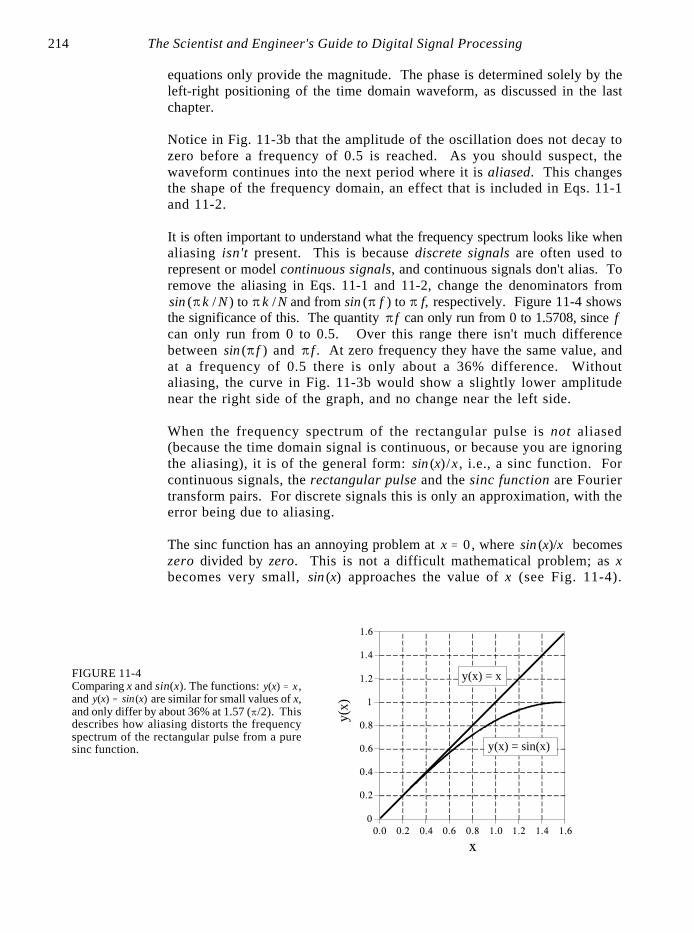
FIGURE 11-4Comparing x and sin(x). The functions: ,y(x) ' xand are similar for small values of x,y(x) ' sin(x)and only differ by about 36% at 1.57 (B/2). Thisdescribes how aliasing distorts the frequencyspectrum of the rectangular pulse from a puresinc function.

y(x)

equations only provide the magnitude. The phase is determined solely by theleft-right positioning of the time domain waveform, as discussed in the lastchapter.

Notice in Fig. 11-3b that the amplitude of the oscillation does not decay tozero before a frequency of 0.5 is reached. As you should suspect, thewaveform continues into the next period where it is aliased. This changesthe shape of the frequency domain, an effect that is included in Eqs. 11-1and 11-2.

It is often important to understand what the frequency spectrum looks like whenaliasing isn't present. This is because discrete signals are often used torepresent or model continuous signals, and continuous signals don't alias. Toremove the aliasing in Eqs. 11-1 and 11-2, change the denominators from

respectively. Figure 11-4 showssin (B k / N ) to B k / N and from sin (B f ) to B f,the significance of this. The quantity can only run from 0 to 1.5708, since B f fcan only run from 0 to 0.5. Over this range there isn't much differencebetween and . At zero frequency they have the same value, andsin (B f ) B fat a frequency of 0.5 there is only about a 36% difference. Withoutaliasing, the curve in Fig. 11-3b would show a slightly lower amplitudenear the right side of the graph, and no change near the left side. When the frequency spectrum of the rectangular pulse is not aliased(because the time domain signal is continuous, or because you are ignoringthe aliasing), it is of the general form: , i.e., a sinc function. Forsin (x)/xcontinuous signals, the rectangular pulse and the sinc function are Fouriertransform pairs. For discrete signals this is only an approximation, with theerror being due to aliasing.

The sinc function has an annoying problem at , where becomesx ' 0 sin (x)/xzero divided by zero. This is not a difficult mathematical problem; as xbecomes very small, approaches the value of x (see Fig. 11-4).sin (x)


EQUATION 11-3Inverse DFT of the rectangular pulse. In thefrequency domain, the pulse has anamplitude of one, and runs from samplenumber 0 through sample number M-1. Theparameter N is the length of the DFT, and

is the time domain signal with i runningx[i]from 0 to N-1. To avoid the division byzero, use .x[0] ' (2M&1)/N

x [ i ] '1N

sin(2B i (M & 1/2) /N )sin(B i /N )

This turns the sinc function into , which has a value of one. In other words,x/xas x becomes smaller and smaller, the value of approaches one, whichsinc (x)includes . Now try to tell your computer this! All it sees is asinc (0) ' 1division by zero, causing it to complain and stop your program. The importantpoint to remember is that your program must include special handling at x ' 0when calculating the sinc function.

A key trait of the sinc function is the location of the zero crossings. Theseoccur at frequencies where an integer number of the sinusoid's cycles fitevenly into the rectangular pulse. For example, if the rectangular pulse is20 points wide, the first zero in the frequency domain is at the frequencythat makes one complete cycle in 20 points. The second zero is at thefrequency that makes two complete cycles in 20 points, etc. This can beunderstood by remembering how the DFT is calculated by correlation. Theamplitude of a frequency component is found by multiplying the timedomain signal by a sinusoid and adding up the resulting samples. If thetime domain waveform is a rectangular pulse of unity amplitude, this is thesame as adding the sinusoid's samples that are within the rectangular pulse.If this summation occurs over an integral number of the sinusoid's cycles,the result will be zero.

The sinc function is widely used in DSP because it is the Fourier transform pairof a very simple waveform, the rectangular pulse. For example, the sincfunction is used in spectral analysis, as discussed in Chapter 9. Consider theanalysis of an infinitely long discrete signal. Since the DFT can only workwith finite length signals, N samples are selected to represent the longer signal.The key here is that "selecting N samples from a longer signal" is the same asmultiplying the longer signal by a rectangular pulse. The ones in therectangular pulse retain the corresponding samples, while the zeros eliminatethem. How does this affect the frequency spectrum of the signal? Multiplyingthe time domain by a rectangular pulse results in the frequency domain beingconvolved with a sinc function. This reduces the frequency spectrum'sresolution, as previously shown in Fig. 9-5a.

Other Transform Pairs

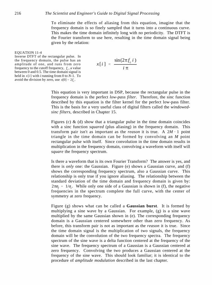
Figure 11-5 (a) and (b) show the duality of the above: a rectangular pulse inthe frequency domain corresponds to a sinc function (plus aliasing) in the timedomain. Including the effects of aliasing, the time domain signal is given by:


EQUATION 11-4Inverse DTFT of the rectangular pulse. Inthe frequency domain, the pulse has anamplitude of one, and runs from zerofrequency to the cutoff frequency, , a valuefcbetween 0 and 0.5. The time domain signal isheld in with i running from 0 to N-1. Tox [i ]avoid the division by zero, use .x[0] ' 2 fc

x [ i ] 'sin(2B fc i )

i B

To eliminate the effects of aliasing from this equation, imagine that thefrequency domain is so finely sampled that it turns into a continuous curve.This makes the time domain infinitely long with no periodicity. The DTFT isthe Fourier transform to use here, resulting in the time domain signal beinggiven by the relation:

This equation is very important in DSP, because the rectangular pulse in thefrequency domain is the perfect low-pass filter. Therefore, the sinc functiondescribed by this equation is the filter kernel for the perfect low-pass filter.This is the basis for a very useful class of digital filters called the windowed-sinc filters, described in Chapter 15.

Figures (c) & (d) show that a triangular pulse in the time domain coincideswith a sinc function squared (plus aliasing) in the frequency domain. Thistransform pair isn't as important as the reason it is true. A point2M& 1triangle in the time domain can be formed by convolving an M pointrectangular pulse with itself. Since convolution in the time domain results inmultiplication in the frequency domain, convolving a waveform with itself willsquare the frequency spectrum.

Is there a waveform that is its own Fourier Transform? The answer is yes, andthere is only one: the Gaussian. Figure (e) shows a Gaussian curve, and (f)shows the corresponding frequency spectrum, also a Gaussian curve. Thisrelationship is only true if you ignore aliasing. The relationship between thestandard deviation of the time domain and frequency domain is given by:

. While only one side of a Gaussian is shown in (f), the negative2BFf ' 1/Ftfrequencies in the spectrum complete the full curve, with the center ofsymmetry at zero frequency.

Figure (g) shows what can be called a Gaussian burst. It is formed bymultiplying a sine wave by a Gaussian. For example, (g) is a sine wavemultiplied by the same Gaussian shown in (e). The corresponding frequencydomain is a Gaussian centered somewhere other than zero frequency. Asbefore, this transform pair is not as important as the reason it is true. Sincethe time domain signal is the multiplication of two signals, the frequencydomain will be the convolution of the two frequency spectra. The frequencyspectrum of the sine wave is a delta function centered at the frequency of thesine wave. The frequency spectrum of a Gaussian is a Gaussian centered atzero frequency. Convolving the two produces a Gaussian centered at thefrequency of the sine wave. This should look familiar; it is identical to theprocedure of amplitude modulation described in the last chapter.


Sample number0 16 32 48 64 80 96 112 128

-1

0

1

2

a. Sinc

127

3

Frequency0 0.1 0.2 0.3 0.4 0.5

-5

0

5

10

15

b. Rectangular pulse

Frequency0 0.1 0.2 0.3 0.4 0.5

-5

0

5

10

15

d. Sinc squared


Sample number0 16 32 48 64 80 96 112 128

-1

0

1

2

c. Triangle

127

Sample number0 16 32 48 64 80 96 112 128

-1

0

1

2

e. Gaussian

127Frequency

0 0.1 0.2 0.3 0.4 0.5-5

0

5

10

15

f. Gaussian

FIGURE 11-5Common transform pairs.

Sample number0 16 32 48 64 80 96 112 128

-2

-1

0

1

2

3

g. Gaussian burst

127Frequency

0 0.1 0.2 0.3 0.4 0.5-5

0

5

10

15

h. Gaussian

Am

plitu

de

Am

plitu

deA

mpl

itude

Am

plitu

deA

mpl

itude

Am

plitu

deA

mpl

itude

Am

plitu

de


Gibbs Effect

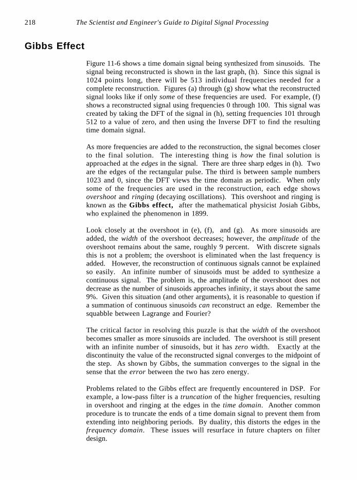
Figure 11-6 shows a time domain signal being synthesized from sinusoids. Thesignal being reconstructed is shown in the last graph, (h). Since this signal is1024 points long, there will be 513 individual frequencies needed for acomplete reconstruction. Figures (a) through (g) show what the reconstructedsignal looks like if only some of these frequencies are used. For example, (f)shows a reconstructed signal using frequencies 0 through 100. This signal wascreated by taking the DFT of the signal in (h), setting frequencies 101 through512 to a value of zero, and then using the Inverse DFT to find the resultingtime domain signal.

As more frequencies are added to the reconstruction, the signal becomes closerto the final solution. The interesting thing is how the final solution isapproached at the edges in the signal. There are three sharp edges in (h). Twoare the edges of the rectangular pulse. The third is between sample numbers1023 and 0, since the DFT views the time domain as periodic. When onlysome of the frequencies are used in the reconstruction, each edge showsovershoot and ringing (decaying oscillations). This overshoot and ringing isknown as the Gibbs effect, after the mathematical physicist Josiah Gibbs,who explained the phenomenon in 1899.

Look closely at the overshoot in (e), (f), and (g). As more sinusoids areadded, the width of the overshoot decreases; however, the amplitude of theovershoot remains about the same, roughly 9 percent. With discrete signalsthis is not a problem; the overshoot is eliminated when the last frequency isadded. However, the reconstruction of continuous signals cannot be explainedso easily. An infinite number of sinusoids must be added to synthesize acontinuous signal. The problem is, the amplitude of the overshoot does notdecrease as the number of sinusoids approaches infinity, it stays about the same9%. Given this situation (and other arguments), it is reasonable to question ifa summation of continuous sinusoids can reconstruct an edge. Remember thesquabble between Lagrange and Fourier?

The critical factor in resolving this puzzle is that the width of the overshootbecomes smaller as more sinusoids are included. The overshoot is still presentwith an infinite number of sinusoids, but it has zero width. Exactly at thediscontinuity the value of the reconstructed signal converges to the midpoint ofthe step. As shown by Gibbs, the summation converges to the signal in thesense that the error between the two has zero energy.

Problems related to the Gibbs effect are frequently encountered in DSP. Forexample, a low-pass filter is a truncation of the higher frequencies, resultingin overshoot and ringing at the edges in the time domain. Another commonprocedure is to truncate the ends of a time domain signal to prevent them fromextending into neighboring periods. By duality, this distorts the edges in thefrequency domain. These issues will resurface in future chapters on filterdesign.


Sample number0 256 512 768 1024

-1

0

1

2

a. Frequencies: 0

1023Sample number

0 256 512 768 1024-1

0

1

2

b. Frequencies: 0 & 1

1023

Sample number0 256 512 768 1024

-1

0

1

2

d. Frequencies: 0 to 10

1023Sample number

0 256 512 768 1024-1

0

1

2

c. Frequencies: 0 to 3

1023

Sample number0 256 512 768 1024

-1

0

1

2

e. Frequencies: 0 to 30

1023Sample number

0 256 512 768 1024-1

0

1

2

f. Frequencies: 0 to 100

1023

FIGURE 11-6.The Gibbs effect.

Sample number0 256 512 768 1024

-1

0

1

2

g. Frequencies: 0 to 300

1023Sample number

0 256 512 768 1024-1

0

1

2

h. Frequencies: 0 to 512

1023

Am

plitu

deA

mpl

itude

Am

plitu

deA

mpl

itude

Am

plitu

deA

mpl

itude

Am

plitu

deA

mpl

itude


Sample number0 128 256 384 512 640 768 896 1024

-2

-1

0

1

2

a. Sine wave

1023Frequency

0 0.02 0.04 0.06 0.08 0.10

100

200

300

400

500

600

700

b. Fundamental

Frequency0 0.02 0.04 0.06 0.08 0.1

0

100

200

300

400

500

600

700

d. Fundamental pluseven and odd harmonics


Sample number0 128 256 384 512 640 768 896 1024

-2

-1

0

1

2

c. Asymmetrical distortion

1023

Sample number0 128 256 384 512 640 768 896 1024

-2

-1

0

1

2

e. Symmetrical distortion

1023Frequency

0 0.02 0.04 0.06 0.08 0.10

100

200

300

400

500

600

700

f. Fundamental plusodd harmonics

FIGURE 11-7Example of harmonics. Asymmetrical distortion, shown in (c), results in even and odd harmonics,(d), while symmetrical distortion, shown in (e), produces only odd harmonics, (f).

Am

plitu

de

Am

plitu

deA

mpl

itude

Am

plitu

de

Am

plitu

deA

mpl

itude

Harmonics

If a signal is periodic with frequency f, the only frequencies composing thesignal are integer multiples of f, i.e., f, 2f, 3f, 4f, etc. These frequencies arecalled harmonics. The first harmonic is f, the second harmonic is 2f, thethird harmonic is 3f, and so forth. The first harmonic (i.e., f) is also givena special name, the fundamental frequency. Figure 11-7 shows an


Sample number0 20 40 60 80 100

-2

-1

0

1

2

a. Distorted sine wave

Frequency0 0.1 0.2 0.3 0.4 0.5

-100

0

100

200

300

400

500

600

700

b. Frequency spectrum

Frequency0 0.1 0.2 0.3 0.4 0.5

-100

-80

-60

-40

-20

0

20

40

60

80

100

c. Frequency spectrum (Log scale)

105

104

103

102

101

100

10-1

10-2

10-3

10-4

10-5


FIGURE 11-8Harmonic aliasing. Figures (a) and (b) showa distorted sine wave and its frequencyspectrum, respectively. Harmonics with afrequency greater than 0.5 will becomealiased to a frequency between 0 and 0.5.Figure (c) displays the same frequencyspectrum on a logarithmic scale, revealingmany aliased peaks with very low amplitude.

Am

plitu

de

Am

plitu

deA

mpl

itude

example. Figure (a) is a pure sine wave, and (b) is its DFT, a single peak.In (c), the sine wave has been distorted by poking in the tops of the peaks.Figure (d) shows the result of this distortion in the frequency domain.Because the distorted signal is periodic with the same frequency as theoriginal sine wave, the frequency domain is composed of the original peakplus harmonics. Harmonics can be of any amplitude; however, they usuallybecome smaller as they increase in frequency. As with any signal, sharpedges result in higher frequencies. For example, consider a common TTLlogic gate generating a 1 kHz square wave. The edges rise in a fewnanoseconds, resulting in harmonics being generated to nearly 100 MHz,the ten-thousandth harmonic!

Figure (e) demonstrates a subtlety of harmonic analysis. If the signal issymmetrical around a horizontal axis, i.e., the top lobes are mirror images ofthe bottom lobes, all of the even harmonics will have a value of zero. Asshown in (f), the only frequencies contained in the signal are the fundamental,the third harmonic, the fifth harmonic, etc.

All continuous periodic signals can be represented as a summation ofharmonics, just as described. Discrete periodic signals have a problem thatdisrupts this simple relation. As you might have guessed, the problem isaliasing. Figure 11-8a shows a sine wave distorted in the same manner asbefore, by poking in the tops of the peaks. This waveform looks much less


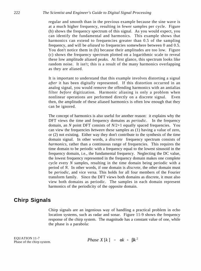
EQUATION 11-7Phase of the chirp system. Phase X [k ] ' "k % $k 2

regular and smooth than in the previous example because the sine wave isat a much higher frequency, resulting in fewer samples per cycle. Figure(b) shows the frequency spectrum of this signal. As you would expect, youcan identify the fundamental and harmonics. This example shows thatharmonics can extend to frequencies greater than 0.5 of the samplingfrequency, and will be aliased to frequencies somewhere between 0 and 0.5.You don't notice them in (b) because their amplitudes are too low. Figure(c) shows the frequency spectrum plotted on a logarithmic scale to revealthese low amplitude aliased peaks. At first glance, this spectrum looks likerandom noise. It isn't; this is a result of the many harmonics overlappingas they are aliased.

It is important to understand that this example involves distorting a signalafter it has been digitally represented. If this distortion occurred in ananalog signal, you would remove the offending harmonics with an antialiasfilter before digitization. Harmonic aliasing is only a problem whennonlinear operations are performed directly on a discrete signal. Eventhen, the amplitude of these aliased harmonics is often low enough that theycan be ignored.

The concept of harmonics is also useful for another reason: it explains why theDFT views the time and frequency domains as periodic. In the frequencydomain, an N point DFT consists of N/2+1 equally spaced frequencies. Youcan view the frequencies between these samples as (1) having a value of zero,or (2) not existing. Either way they don't contribute to the synthesis of the timedomain signal. In other words, a discrete frequency spectrum consists ofharmonics, rather than a continuous range of frequencies. This requires thetime domain to be periodic with a frequency equal to the lowest sinusoid in thefrequency domain, i.e., the fundamental frequency. Neglecting the DC value,the lowest frequency represented in the frequency domain makes one completecycle every N samples, resulting in the time domain being periodic with aperiod of N. In other words, if one domain is discrete, the other domain mustbe periodic, and vice versa. This holds for all four members of the Fouriertransform family. Since the DFT views both domains as discrete, it must alsoview both domains as periodic. The samples in each domain representharmonics of the periodicity of the opposite domain.

Chirp Signals

Chirp signals are an ingenious way of handling a practical problem in echolocation systems, such as radar and sonar. Figure 11-9 shows the frequencyresponse of the chirp system. The magnitude has a constant value of one, whilethe phase is a parabola:


Frequency0 0.1 0.2 0.3 0.4 0.5

-1

0

1

2

a. Chirp magnitude

Frequency0 0.1 0.2 0.3 0.4 0.5

-200

-150

-100

-50

0

50

b. Chirp phase

Phas

e (r

adia

ns)

Am

plitu

de

FIGURE 11-9Frequency response of the chirp system. The magnitude is a constant, while the phase is a parabola.

Sample number0 20 40 60 80 100 120

-0.5

0

0.5

1

1.5

b. Impulse Response(chirp signal)

Sample number0 20 40 60 80 100 120

-0.5

0

0.5

1

1.5

a. Impulse

FIGURE 11-10The chirp system. The impulse response of a chirp system is a chirp signal.

SystemChirp

Am

plitu

de

Am

plitu

de

The parameter " introduces a linear slope in the phase, that is, it simply shiftsthe impulse response left or right as desired. The parameter $ controls thecurvature of the phase. These two parameters must be chosen such that thephase at frequency 0.5 (i.e. k = N/2) is a multiple of 2B. Remember, wheneverthe phase is directly manipulated, frequency 0 and 0.5 must both have a phaseof zero (or a multiple of 2B, which is the same thing).

Figure 11-10 shows an impulse entering a chirp system, and the impulseresponse exiting the system. The impulse response is an oscillatory burst thatstarts at a low frequency and changes to a high frequency as time progresses. This is called a chirp signal for a very simple reason: it sounds like the chirpof a bird when played through a speaker.

The key feature of the chirp system is that it is completely reversible. If yourun the chirp signal through an antichirp system, the signal is again made intoan impulse. This requires the antichirp system to have a magnitude of one,and the opposite phase of the chirp system. As discussed in the last


chapter, this means that the impulse response of the antichirp system is foundby preforming a left-for-right flip of the chirp system's impulse response.Interesting, but what is it good for?

Consider how a radar system operates. A short burst of radio frequency energyis emitted from a directional antenna. Aircraft and other objects reflect someof this energy back to a radio receiver located next to the transmitter. Sinceradio waves travel at a constant rate, the elapsed time between the transmittedand received signals provides the distance to the target. This brings up thefirst requirement for the pulse: it needs to be as short as possible. Forexample, a 1 microsecond pulse provides a radio burst about 300 meters long.This means that the distance information we obtain with the system will havea resolution of about this same length. If we want better distance resolution,we need a shorter pulse.

The second requirement is obvious: if we want to detect objects farther away,you need more energy in your pulse. Unfortunately, more energy and shorterpulse are conflicting requirements. The electrical power needed to provide apulse is equal to the energy of the pulse divided by the pulse length. Requiringboth more energy and a shorter pulse makes electrical power handling alimiting factor in the system. The output stage of a radio transmitter can onlyhandle so much power without destroying itself.

Chirp signals provide a way of breaking this limitation. Before the impulsereaches the final stage of the radio transmitter, it is passed through a chirpsystem. Instead of bouncing an impulse off the target aircraft, a chirp signalis used. After the chirp echo is received, the signal is passed through anantichirp system, restoring the signal to an impulse. This allows the portionsof the system that measure distance to see short pulses, while the powerhandling circuits see long duration signals. This type of waveshaping is afundamental part of modern radar systems.

delta function pairs - dspguide.com

Documents