delft university of technology model-based optimization of
TRANSCRIPT

Delft University of Technology
Model-based optimization of oil and gas production (PPT)
Jansen, Jan Dirk
Publication date2017Document VersionFinal published versionCitation (APA)Jansen, J. D. (2017). Model-based optimization of oil and gas production (PPT). IPAM Workshop onComputational Issues in Oil Field Applications Tutorials, Los Angeles, United States.
Important noteTo cite this publication, please use the final published version (if applicable).Please check the document version above.
CopyrightOther than for strictly personal use, it is not permitted to download, forward or distribute the text or part of it, without the consentof the author(s) and/or copyright holder(s), unless the work is under an open content license such as Creative Commons.
Takedown policyPlease contact us and provide details if you believe this document breaches copyrights.We will remove access to the work immediately and investigate your claim.
This work is downloaded from Delft University of Technology.For technical reasons the number of authors shown on this cover page is limited to a maximum of 10.
IPAM 2017 - Computational Issues in Oil Field Applications 1
Model-based optimization ofoil and gas production
Jan Dirk JansenDelft University of Technology
IPAM Long ProgramComputational Issues in Oil Field Applications - Tutorials
UCLA, 21-24 March 2017

IPAM 2017 - Computational Issues in Oil Field Applications 2
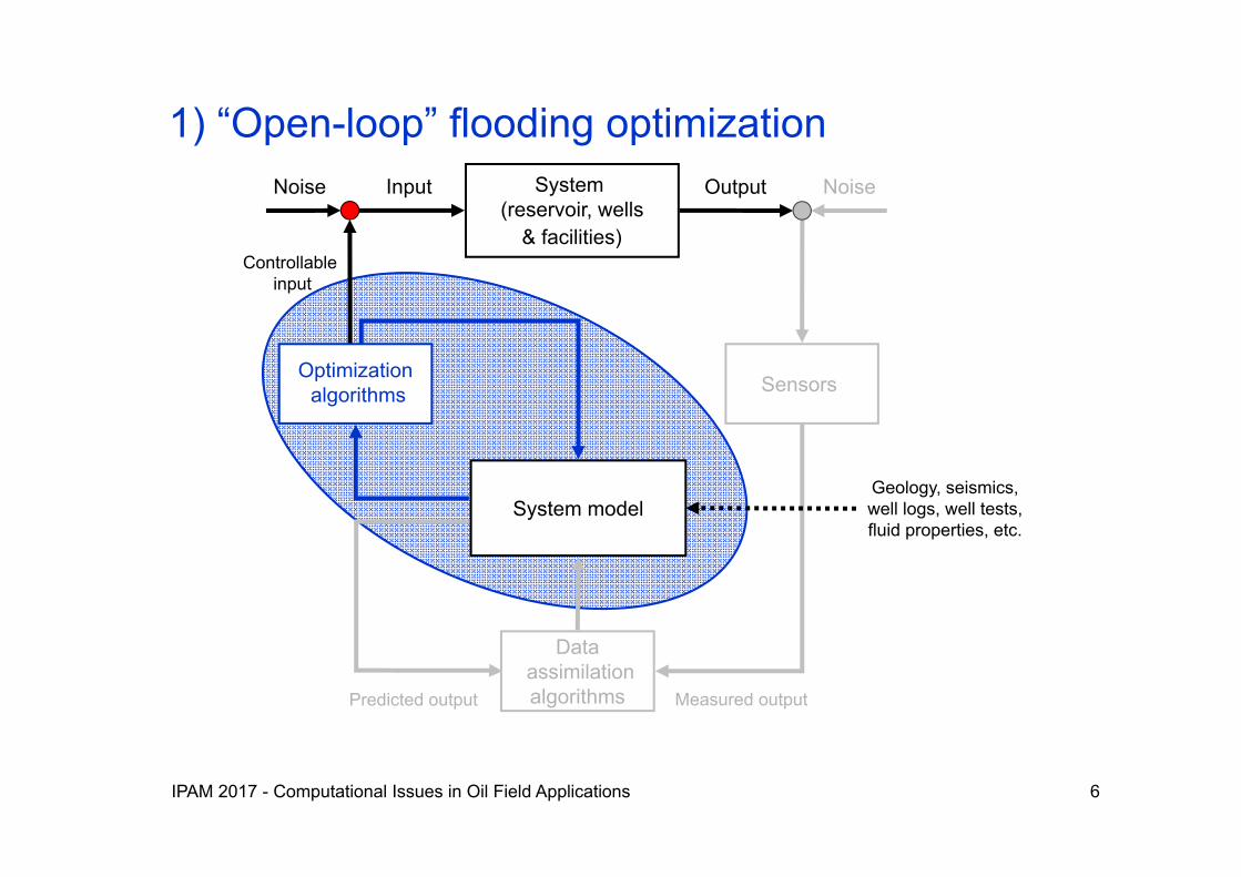
Dataassimilationalgorithms
Noise OutputInput NoiseSystem (reservoir, wells
& facilities)
Optimizationalgorithms Sensors
System models
Predicted output Measured output
Controllableinput
Geology, seismics,well logs, well tests,fluid properties, etc.
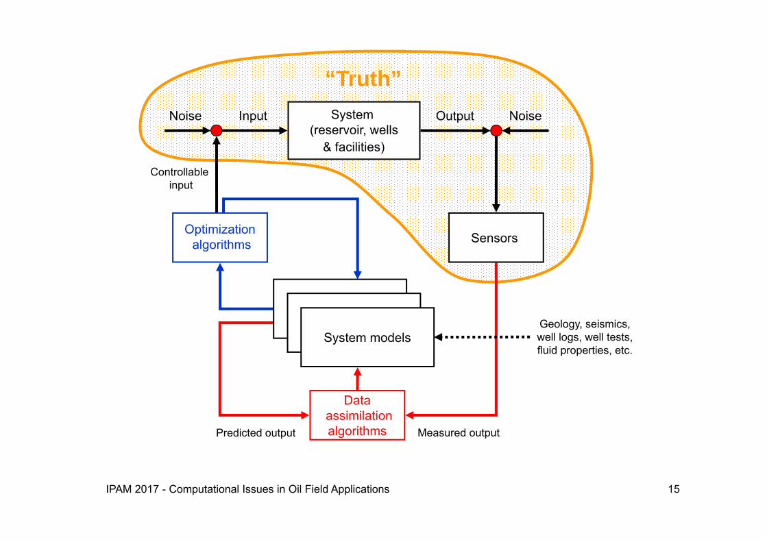
Closed-loop reservoir management
IPAM 2017 - Computational Issues in Oil Field Applications 3
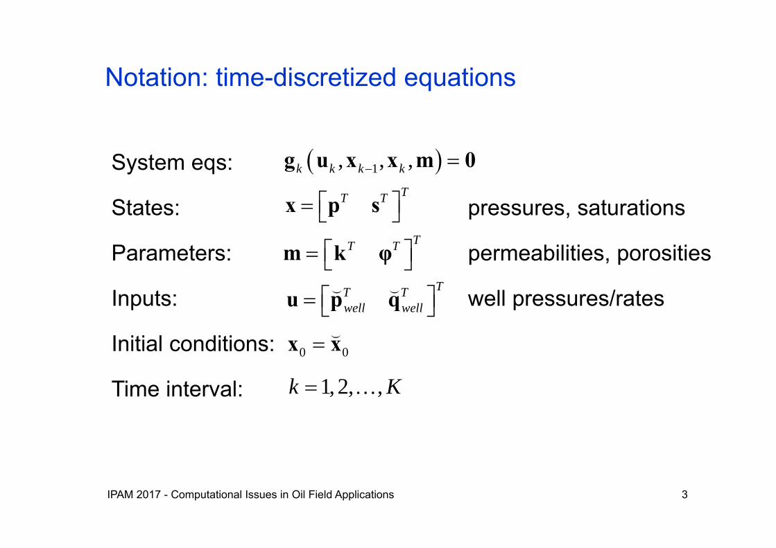
System eqs:
States: pressures, saturations
Parameters: permeabilities, porosities
Inputs: well pressures/rates
Initial conditions:
Time interval:
Notation: time-discretized equations
1, , ,k k k k g u x x m 0
0 0x x
1,2, ,k K
TT T x p sTT T m k φ
TT Twell well u p q
IPAM 2017 - Computational Issues in Oil Field Applications 4
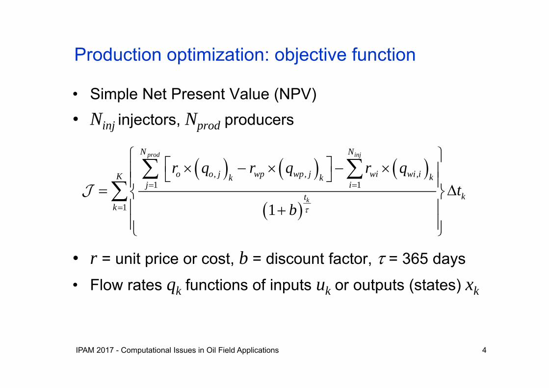
Production optimization: objective function
• Simple Net Present Value (NPV)• Ninj injectors, Nprod producers
• r = unit price or cost, b = discount factor, = 365 days
• Flow rates qk functions of inputs uk or outputs (states) xk
, , ,1 1
1 1
prod inj
k
N N
o o j wp wp j wi wi iK kk kj i
ktk
r q r q r qt
b
IPAM 2017 - Computational Issues in Oil Field Applications 5
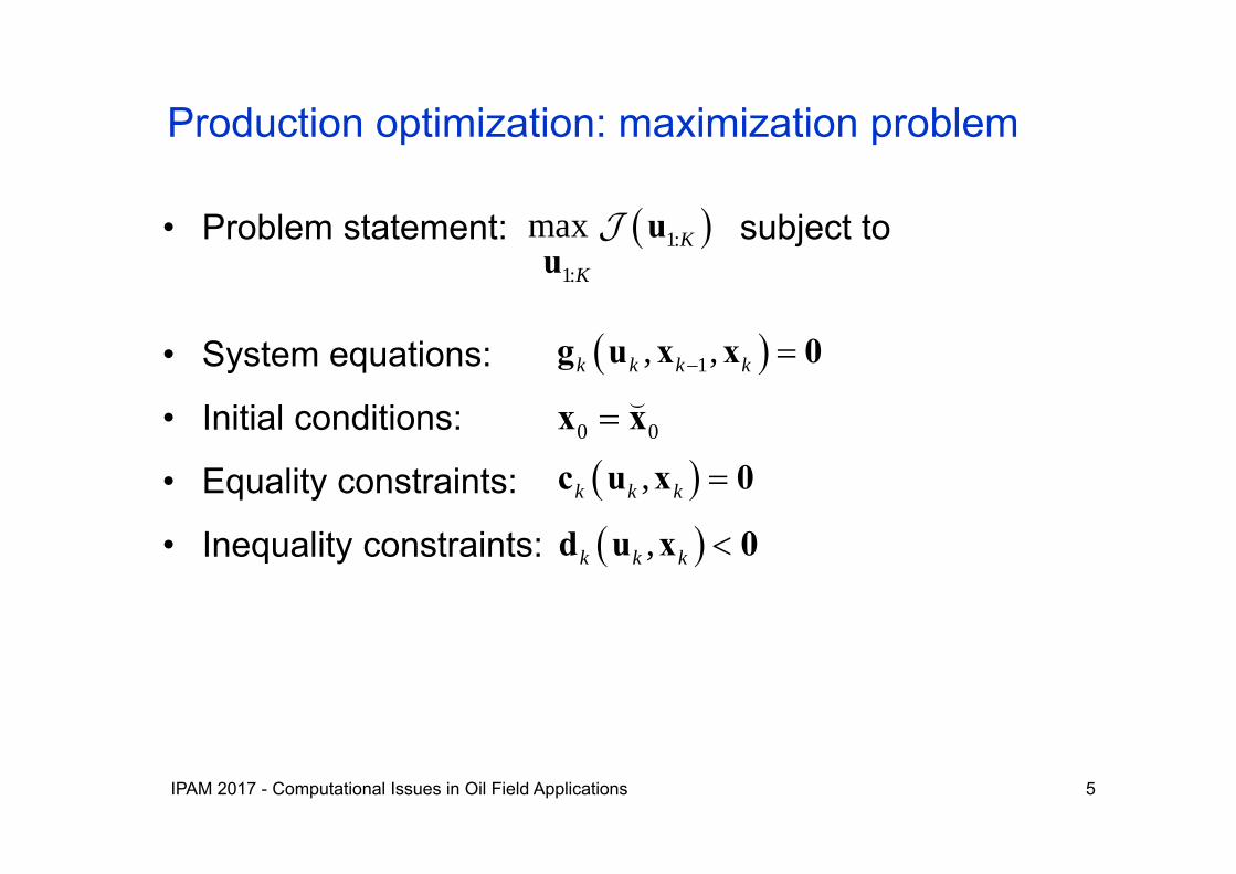
Production optimization: maximization problem
• Problem statement: subject to
• System equations:
• Initial conditions:
• Equality constraints:
• Inequality constraints:
1:
1:
max K
K
uu
,k k k c u x 0
1, ,k k k k g u x x 0
0 0 x x
,k k k d u x 0
IPAM 2017 - Computational Issues in Oil Field Applications 6
Dataassimilationalgorithms
Noise OutputInput NoiseSystem (reservoir, wells
& facilities)
Optimizationalgorithms Sensors
System model
Predicted output Measured output
Controllableinput
Geology, seismics,well logs, well tests,fluid properties, etc.
1) “Open-loop” flooding optimization
IPAM 2017 - Computational Issues in Oil Field Applications 7
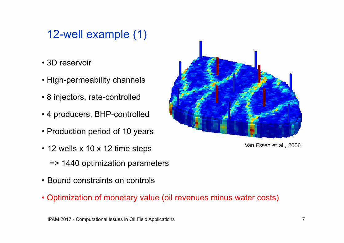
• 3D reservoir
• High-permeability channels
• 8 injectors, rate-controlled
• 4 producers, BHP-controlled
• Production period of 10 years
• 12 wells x 10 x 12 time steps
=> 1440 optimization parameters
• Bound constraints on controls
• Optimization of monetary value (oil revenues minus water costs)
Van Essen et al., 2006
12-well example (1)
IPAM 2017 - Computational Issues in Oil Field Applications 8
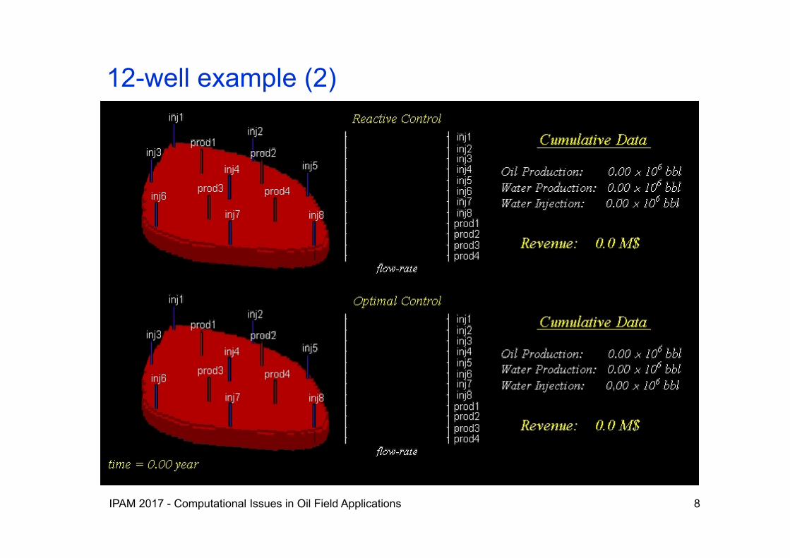
12-well example (2)

IPAM 2017 - Computational Issues in Oil Field Applications 9
12-well example (3)

IPAM 2017 - Computational Issues in Oil Field Applications 10
• Real wells are sparse and far apart• Real wells have more complicated constraints• Field management is usually production-focused• Long-term optimization may jeopardize short-term profit• Production engineers don’t trust reservoir models anyway
• We do not know the reservoir!
Why this wouldn’t work

IPAM 2017 - Computational Issues in Oil Field Applications 11
Dataassimilationalgorithms
Noise OutputInput NoiseSystem (reservoir, wells
& facilities)
Optimizationalgorithms Sensors
System models
Predicted output Measured output
Controllableinput
Geology, seismics,well logs, well tests,fluid properties, etc.
2) “Robust” open-loop flooding optimization
IPAM 2017 - Computational Issues in Oil Field Applications 12
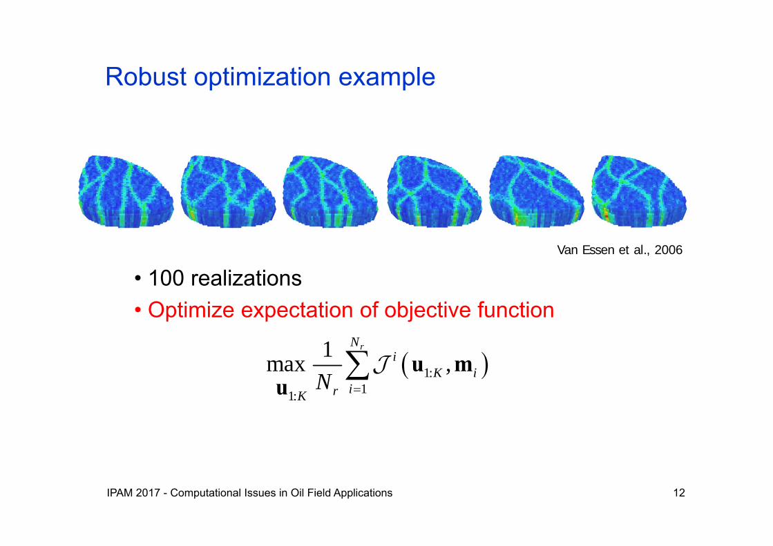
• 100 realizations• Optimize expectation of objective function
Van Essen et al., 2006
1:11:
1max ,rN
iK i
irKN u m
u
Robust optimization example

IPAM 2017 - Computational Issues in Oil Field Applications 13
3 control strategies applied to set of 100 realizations:reactive control, nominal optimization, robust optimization
Van Essen et al., 2006
Robust optimization results

IPAM 2017 - Computational Issues in Oil Field Applications 14
Dataassimilationalgorithms
Noise OutputInput NoiseSystem (reservoir, wells
& facilities)
Optimizationalgorithms Sensors
System models
Predicted output Measured output
Controllableinput
Geology, seismics,well logs, well tests,fluid properties, etc.
3) Closed-loop flooding optimization
IPAM 2017 - Computational Issues in Oil Field Applications 15
“Truth”
Dataassimilationalgorithms
Noise OutputInput NoiseSystem (reservoir, wells
& facilities)
Optimizationalgorithms Sensors
System models
Predicted output Measured output
Controllableinput
Geology, seismics,well logs, well tests,fluid properties, etc.
IPAM 2017 - Computational Issues in Oil Field Applications 16
1 2 3 4 5 68.5
9
9.5
10
10.5x 10⁷N
PV, $
1 2 3 4 5 6-2
-1.5
-1.0
-0.5
0
Dis
coun
ted
wat
er c
osts
, $
1 2 3 4 5 68.5
9
9.5
10
10.5x 10⁷
Dis
coun
ted
oil r
even
ues,
$
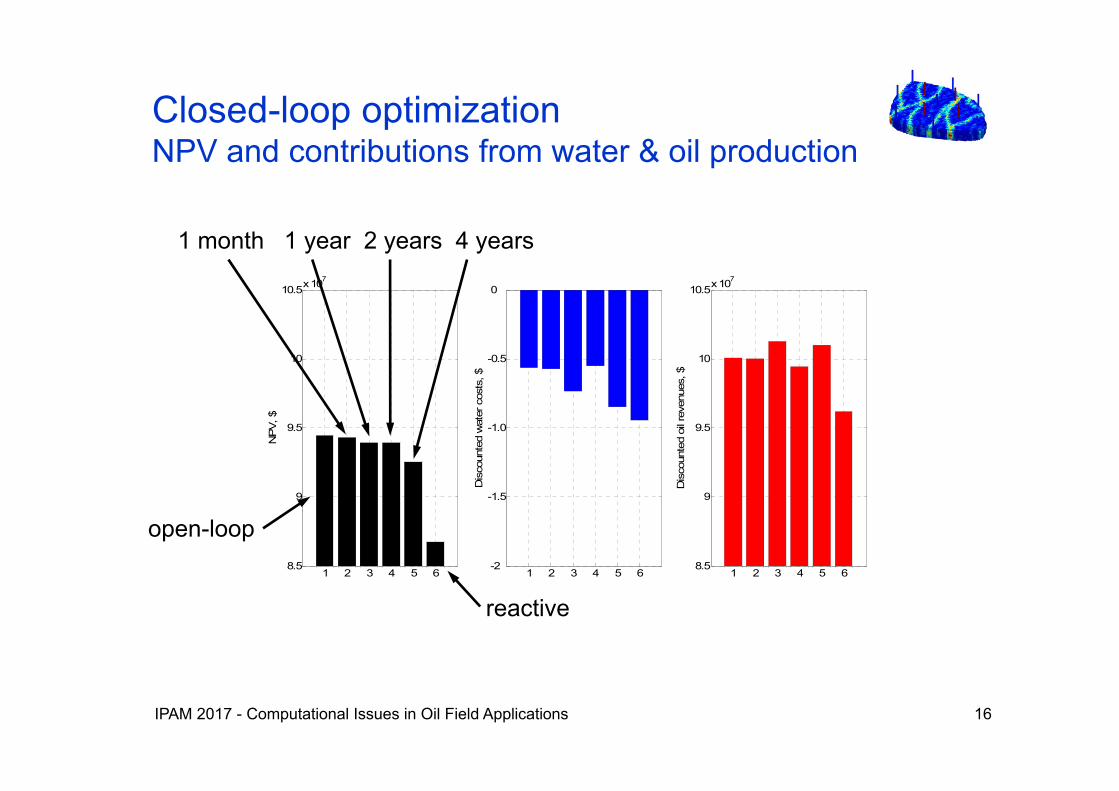
reactive
open-loop
1 month 1 year 2 years 4 years
Closed-loop optimizationNPV and contributions from water & oil production

IPAM 2017 - Computational Issues in Oil Field Applications 17
• Global versus local• Gradient-based versus gradient-free• Constrained versus non-constrained• ‘Classical’ versus ‘non-classical’
(simulated annealing, particle swarms, etc.)• We use ‘optimal control theory’ or ‘adjoint-based’
optimization• Has been proposed for history matching (Chen et al.
1974, Chavent et al. 1975, Li, Reynolds and Oliver 2003) and for flooding optimization (Ramirez 1987, Asheim1988, Virnovski 1991, Zakirov et al. 1996, Sudaryantoand Yortsos, 2000, Brouwer and Jansen 2004, Sarma et al. 2004)
Optimization techniques
IPAM 2017 - Computational Issues in Oil Field Applications 18
• Gradient based optimization technique – local optimum• Gradients of objective function with respect to controls
obtained from ‘adjoint’ equation • Gradients can be used with steepest ascent, quasi Newton,
or trust-region methods • Results in dynamic control strategy, i.e. controls change
over time• Computational effort independent of number of controls• Output constraints not trivial; various techniques used• Implementation is code-intrusive
Optimal control theory, summary

IPAM 2017 - Computational Issues in Oil Field Applications 19
Adjoint-Based Optimization
Part 1 - Theory

IPAM 2017 - Computational Issues in Oil Field Applications 20
22u u
uObjective function
Unconstrained optimization (1D)
2
2 4 0 minimumu
04 0 0
uu
u
IPAM 2017 - Computational Issues in Oil Field Applications 21
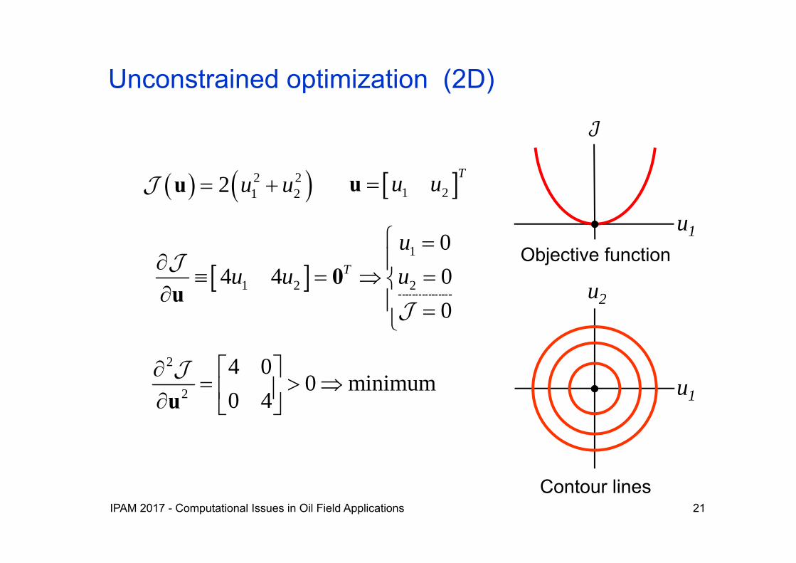
2 21 22 u u u
u1
u2
Contour lines
u1
Objective function
Unconstrained optimization (2D)
2
2
4 00 minimum
0 4
u
1
1 2 2
04 4 0
0
T
uu u u
0u
1 2Tu uu
IPAM 2017 - Computational Issues in Oil Field Applications 22
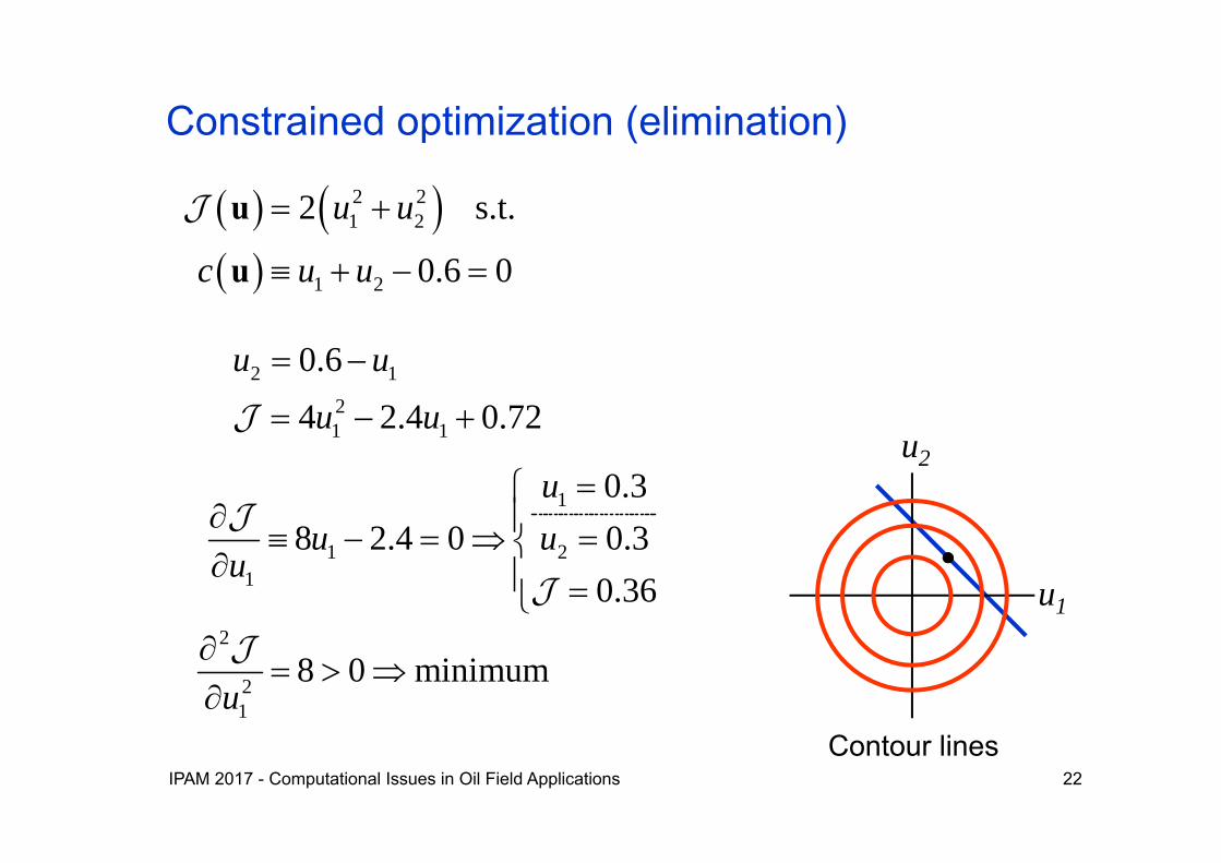
Constrained optimization (elimination)
2
21
8 0 minimumu
2 21 2
1 2
2 s.t.
0.6 0
u u
c u u
u
u
u1
u2
Contour lines
2 121 1
0.6
4 2.4 0.72
u u
u u
1
1 21
0.38 2.4 0 0.3
0.36
uu u
u

IPAM 2017 - Computational Issues in Oil Field Applications 23
second-order conditions more complex
Constrained optimization (Lagrange multipliers)
2 21 2
1 2
2 s.t.
0.6 0
u u
c u u
u
u
2 2
1 2 1 22 0.6
c
u u u u
u u u
1
21 2 1 2
0.30.3
4 4 0.6 1.20.36
T
uu
u u u u
0u
1 2Tu u u

IPAM 2017 - Computational Issues in Oil Field Applications 24
Recall elimination:
What if u2 cannot be expressed in u1 or v.v.?
Consider the total differential:
But how do we compute ?
Lagrange multipliers – interpretation (a)
2
1 1 2 1
uddu u u u
2 21 2
1 2
2 s.t.
0.6 0
u u
c u u
u
u
2 1
21 1 1
0.6
4 2.4 0.72
u u
u u u
2 1u u
IPAM 2017 - Computational Issues in Oil Field Applications 25
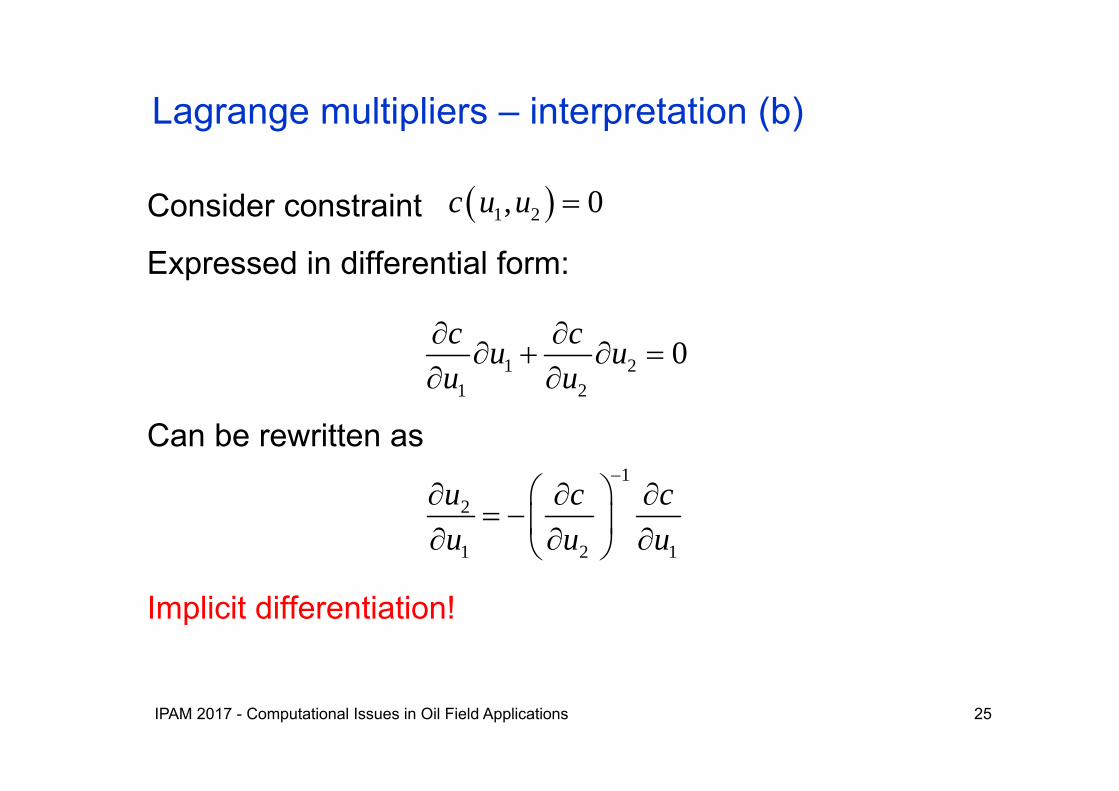
Consider constraint
Expressed in differential form:
Can be rewritten as
Implicit differentiation!
Lagrange multipliers – interpretation (b)
1 21 2
0c cu uu u
1
2
1 2 1
u c cu u u
1 2, 0c u u

IPAM 2017 - Computational Issues in Oil Field Applications 26
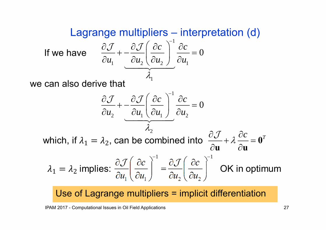
which, in an optimum, can also be written as
1
1 2 2 1
1
0c cu u u u
Lagrange multipliers – interpretation (c)
1
1 1 2 2 1
d c cdu u u u u
we can now write
2
1 1 2 1
uddu u u u
1
2
1 2 1
u c cu u u
Given and
1
0ddu
IPAM 2017 - Computational Issues in Oil Field Applications 27
1
1 2 2 1
1
0c cu u u u
If we have
Lagrange multipliers – interpretation (d)
1
2 1 1 2
2
0c cu u u u
we can also derive that
Tc
0
u u
1 1
1 1 2 2
c cu u u u
Use of Lagrange multipliers = implicit differentiation

IPAM 2017 - Computational Issues in Oil Field Applications 28
Back to the real thing: Production optimization
• Problem statement: subject to
• System equations:
• Initial conditions:
• Equality constraints:
• Inequality constraints:
• As a first step: disregard constraints ck and dk
1:
1:
max K
K
uu
1, ,k k k k g u x x 0
0 0 x x
,k k k c u x 0
,k k k d u x 0

IPAM 2017 - Computational Issues in Oil Field Applications 29
Gradient with implicit differentiation?
Kj jk
j kk k j k
dd
xu u x u
What we are looking for:
Contributions from time steps k…K
Effect of uk on allsubsequent time steps
1 2 1
1 2 1
j j j k k k
k j j k k k
x x x x x xu x x x x u
Requires a lot of implicit differentiation…

IPAM 2017 - Computational Issues in Oil Field Applications 30
• “Adjoin” constraints to objective function:
• Proceed as before: take first derivatives w.r.t. all independent variables and equate them to zero(i.e. force optimality conditions)
• Note that we can write: (index shift)
Gradient with Lagrange multipliers
1: 0: 0: 0 0 0 11
1
,
, ,
, ,
k k kK
TK K K k
k Tk k k k k
u x
u x λ λ x x
λ g u x x
1
1
k k
k k
g gx x
‘Modified objective function’
IPAM 2017 - Computational Issues in Oil Field Applications 31
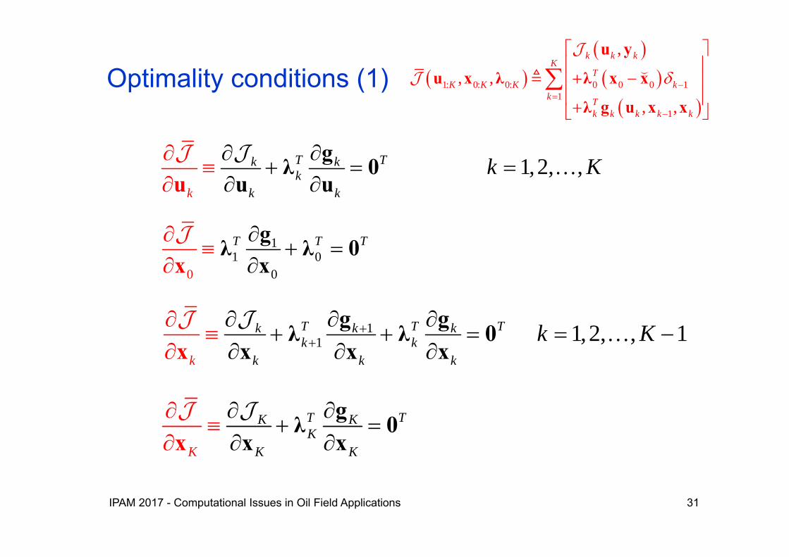
Optimality conditions (1)
1,2, ,T Tk
k
kk
k k
k K
gλ 0u uu
11 0
00
T T T
gλ λx
0x
11 1,2, , 1T T Tk k k
k kk kk k
k K
g gλ λ 0x x xx
K
T TK KK
K K
x
gλ 0x x
1: 0: 0: 0 0 0 11
1
,
, ,
, ,
k k kK
TK K K k
k Tk k k k k
u y
u x λ λ x x
λ g u x x

IPAM 2017 - Computational Issues in Oil Field Applications 32
(Just recovers the initial conditions and system equations)
• The optimality conditions form a joint set of equations for the unknowns
• Can in theory be solved simultaneously (Wathen et al.) but are usually treated sequentially.
Optimality conditions (2)
00
0T T
λx x 0
1, , 1,2, ,T Tk k k k
k
k K
g u x x 0λ
1: 0: 0: 0 0 0 11
1
,
, ,
, ,
k k kK
TK K K k
k Tk k k k k
u y
u x λ λ x x
λ g u x x
1: 0: 0:, ,K K Ku x λ

IPAM 2017 - Computational Issues in Oil Field Applications 33
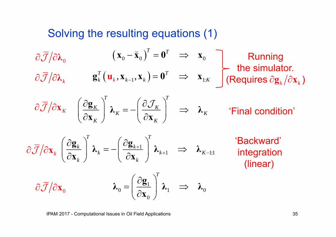
Solving the resulting equations (1)
0 0 0T T x x 0 x
1 1:, ,T Tk k k k K g u x x 0 x
Runningthe simulator.
(Requires )k k g x
0 λ
k λ
Initial guess!

IPAM 2017 - Computational Issues in Oil Field Applications 34
Solving the resulting equations (1)
0 0 0T T x x 0 x
1 1:, ,kT Tk k k K g x 0 xu x
T TK KK
K K
gλ 0
x x
Runningthe simulator.
(Requires )k k g x
0 λ
k λ
K x
IPAM 2017 - Computational Issues in Oil Field Applications 35
0 0 0T T x x 0 x
1 1:, ,kT Tk k k K g x 0 xu x
11 1:1
T T
k kk k K
k k
g gλ λ λx x
10 1 0
0
T
gλ λ λx
T T
K KK K
K K
g λ λx x
‘Final condition’
‘Backward’integration
(linear)
Runningthe simulator.
(Requires )k k g x
0 λ
k λ
K x
k x
0 x
Solving the resulting equations (1)

IPAM 2017 - Computational Issues in Oil Field Applications 36
Solving the resulting equations (2)
???T Tk kk
k k
g 0u
λu
k u Usually not!

IPAM 2017 - Computational Issues in Oil Field Applications 37
Solving the resulting equations (2)
Kj jk
j kk j kk
dd
x
u yu u
!!!k k
dd
u u
Just what we need
Can now be used, e.g., in steepest ascent:
1T
i ik k i
k
dd
u u
u
Recall
Tk kk
kk k
gλu u u
IPAM 2017 - Computational Issues in Oil Field Applications 38
• Adjoint ~ implicit differentiation • Computational effort independent of number of controls• Gradient-based optimization – local optimum• Constraint handling: GRG, lumping, SQP, augmented
Lagrangian, … ; not trivial• Beautiful, but code-intrusive and requires lots of
programming => automatic differentiation • Available in Eclipse (limited functionality), AD-GPRS,
MRST, proprietary simulators• Alternatives: ensemble methods (EnOpt, StoSAG),
streamline-based methods, ‘non classical methods’(particle swarm, etc.; often in combination with ‘proxies’ to reduce computational effort)
Summary adjoint-based optimization

IPAM 2017 - Computational Issues in Oil Field Applications 39
Adjoint-Based Optimization
Part 2 - Examples
IPAM 2017 - Computational Issues in Oil Field Applications 40
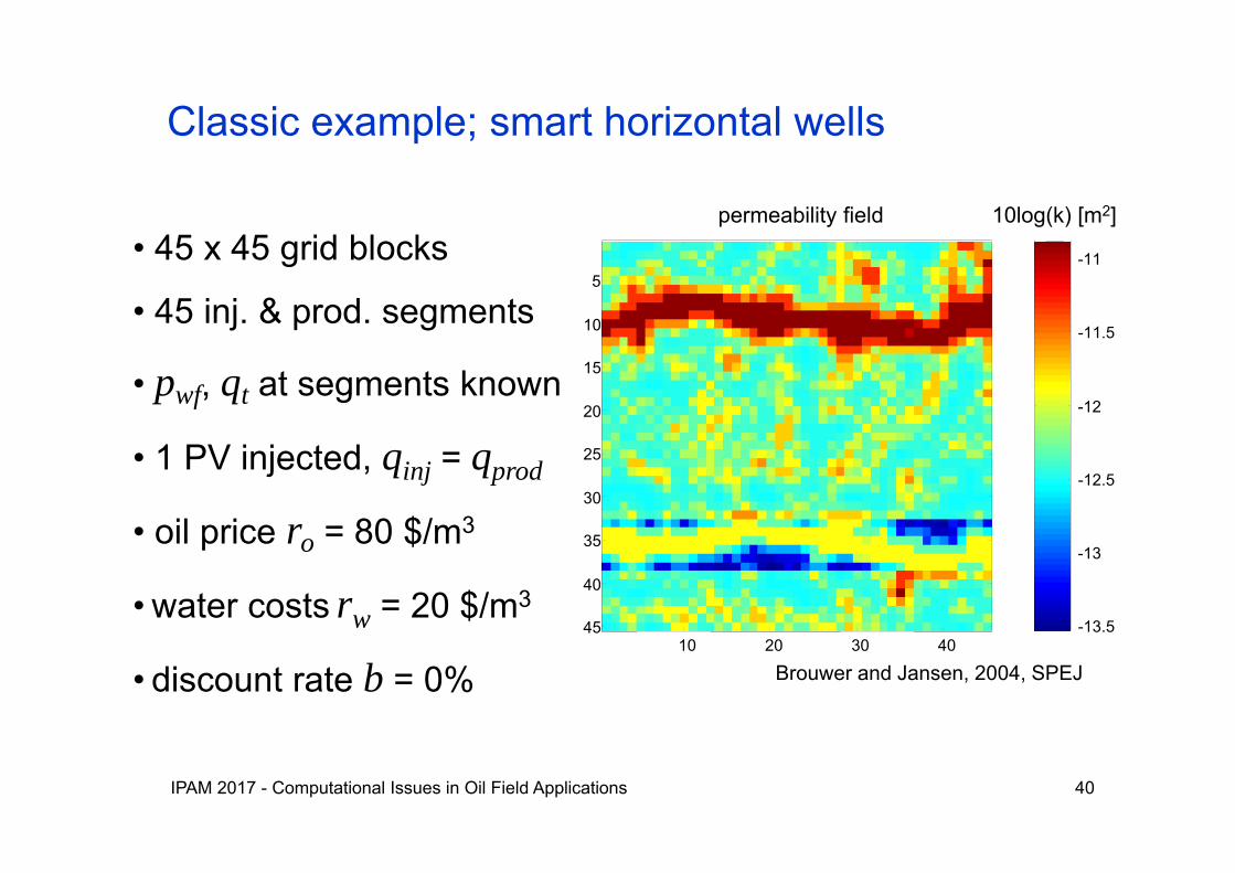
• 45 x 45 grid blocks
• 45 inj. & prod. segments
• pwf, qt at segments known
• 1 PV injected, qinj = qprod
• oil price ro = 80 $/m3
• water costs rw = 20 $/m3
• discount rate b = 0%
-13.5
-13
-12.5
-12
-11.5
-11
permeability field
10 20 30 40
5
10
15
20
25
30
35
40
45
10log(k) [m2]
Brouwer and Jansen, 2004, SPEJ
Classic example; smart horizontal wells

IPAM 2017 - Computational Issues in Oil Field Applications 41
0 100 200 300 400 500 600 7000
200
400
600
800
rate
s [m
3/d]
cum time [d]
water, oil and liquid production rates (m3/d) as function of time
0 100 200 300 400 500 600 7000
1
2
3
4
5x 10⁵
cum
. pro
duct
ion
[m3]
cum time [d]
cumulative water, oil and liquid production (m3) as function of time
ref watref liqref oilopt watopt watopt oil
0
0.1
0.2
0.3
0.4
0.5
0.6
0.7
0.8
0.9
1
5 10 15 20 25 30 35 40 45
5
10
15
20
25
30
35
40
45 0
0.1
0.2
0.3
0.4
0.5
0.6
0.7
0.8
0.9
1
5 10 15 20 25 30 35 40 45
5
10
15
20
25
30
35
40
45 0
0.1
0.2
0.3
0.4
0.5
0.6
0.7
0.8
0.9
1
5 10 15 20 25 30 35 40 45
5
10
15
20
25
30
35
40
45 0
0.1
0.2
0.3
0.4
0.5
0.6
0.7
0.8
0.9
1
5 10 15 20 25 30 35 40 45
5
10
15
20
25
30
35
40
45
Equal pressures in all injector/producer segments
Results; conventional production
IPAM 2017 - Computational Issues in Oil Field Applications 42
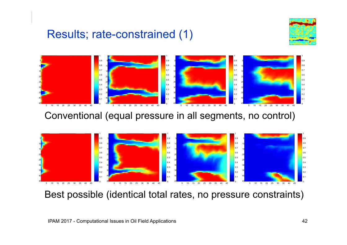
Conventional (equal pressure in all segments, no control)0
0.1
0.2
0.3
0.4
0.5
0.6
0.7
0.8
0.9
1
5 10 15 20 25 30 35 40 45
5
10
15
20
25
30
35
40
45 0
0.1
0.2
0.3
0.4
0.5
0.6
0.7
0.8
0.9
1
5 10 15 20 25 30 35 40 45
5
10
15
20
25
30
35
40
45 0
0.1
0.2
0.3
0.4
0.5
0.6
0.7
0.8
0.9
1
5 10 15 20 25 30 35 40 45
5
10
15
20
25
30
35
40
45 0
0.1
0.2
0.3
0.4
0.5
0.6
0.7
0.8
0.9
1
5 10 15 20 25 30 35 40 45
5
10
15
20
25
30
35
40
45
0
0.1
0.2
0.3
0.4
0.5
0.6
0.7
0.8
0.9
1
5 10 15 20 25 30 35 40 45
5
10
15
20
25
30
35
40
45 0
0.1
0.2
0.3
0.4
0.5
0.6
0.7
0.8
0.9
1
5 10 15 20 25 30 35 40 45
5
10
15
20
25
30
35
40
45 0
0.1
0.2
0.3
0.4
0.5
0.6
0.7
0.8
0.9
1
5 10 15 20 25 30 35 40 45
5
10
15
20
25
30
35
40
45 0
0.1
0.2
0.3
0.4
0.5
0.6
0.7
0.8
0.9
1
5 10 15 20 25 30 35 40 45
5
10
15
20
25
30
35
40
45
Best possible (identical total rates, no pressure constraints)
Results; rate-constrained (1)
IPAM 2017 - Computational Issues in Oil Field Applications 43
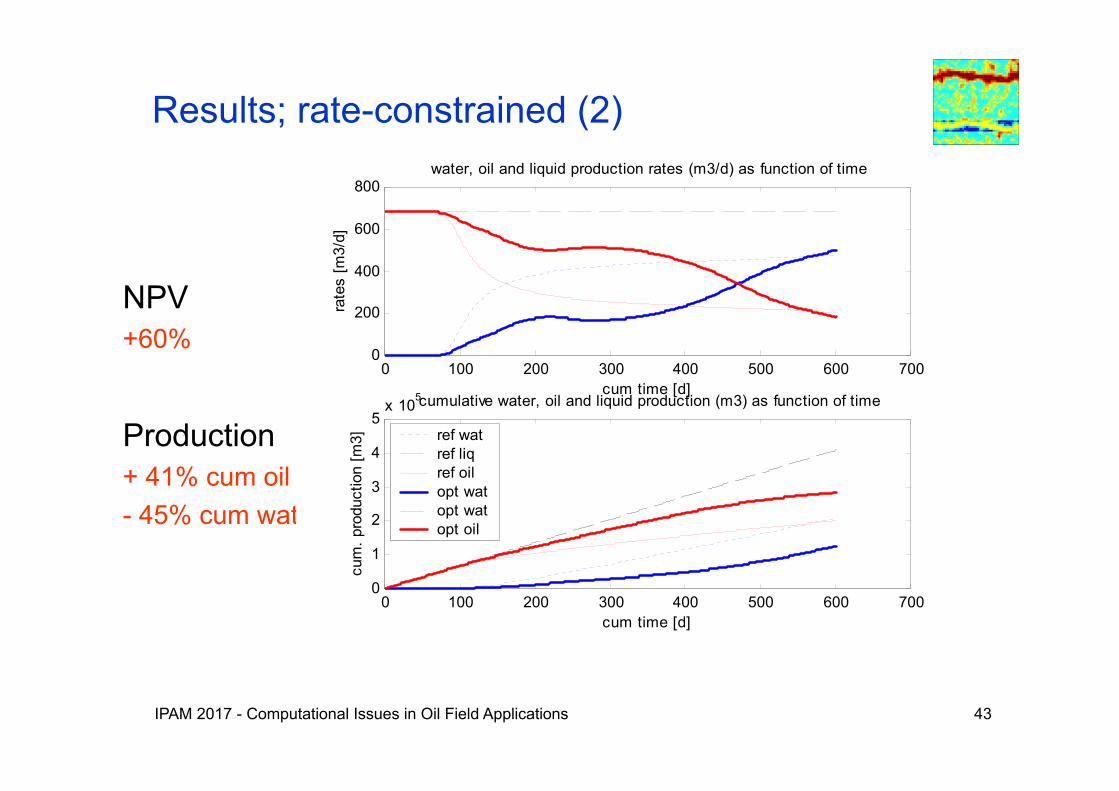
NPV+60%
Production+ 41% cum oil- 45% cum water
0 100 200 300 400 500 600 7000
200
400
600
800
rate
s [m
3/d]
cum time [d]
water, oil and liquid production rates (m3/d) as function of time
0 100 200 300 400 500 600 7000
1
2
3
4
5x 10⁵
cum
. pro
duct
ion
[m3]
cum time [d]
cumulative water, oil and liquid production (m3) as function of time
ref watref liqref oilopt watopt watopt oil
Results; rate-constrained (2)

IPAM 2017 - Computational Issues in Oil Field Applications 44
• Limited energy available • Total injection/production rate dependent on number of
active wells
Pressure-constrained operation

IPAM 2017 - Computational Issues in Oil Field Applications 45
0 100 200 300 400 500 600 7000
200
400
600
800
rate
s [m
3]cum time [d]
water, oil and liquid production rates (m3/d) as function of time
0 100 200 300 400 500 600 7000
1
2
3
4
5x 10⁵
cum
. pro
duct
ion
[m3]
cum time [d]
cumulative water, oil and liquid production (m3) as function of time
ref watref liqref oilopt watopt liqopt oil
Improvementin NPV+53%
Production+16% cum oil-77% cum water
Injection-32% cum water
Results: pressure-constrained

IPAM 2017 - Computational Issues in Oil Field Applications 46
0
0.1
0.2
0.3
0.4
0.5
0.6
0.7
0.8
0.9
1
cum time [yr]
wel
l num
ber
inj. valve setting vs. time for all wells
5
10
15
20
25
30
35
40
45 0
0.1
0.2
0.3
0.4
0.5
0.6
0.7
0.8
0.9
1
cum time [yr]
wel
l num
ber
prod. valve setting vs. time for all wells
5
10
15
20
25
30
35
40
45
Optimum valve-settings (1)
100 200 300 400 500 600 700 800 9000
0.2
0.4
0.6
0.8
1
valv
e-se
tting
optimum valve-position for injector segment 12 as function of time step
0 0.1 0.2 0.3 0.4 0.5 0.6 0.7 0.8 0.9 1time step (n)
inje
ct s
egm
12
optimum valve-position for injector segment 12 as function of time step
100 200 300 400 500 600 700 800 900
12
12
12
• Bang-bang (on-off) solution• Necessary condition: linear controls, linear constraints
IPAM 2017 - Computational Issues in Oil Field Applications 47
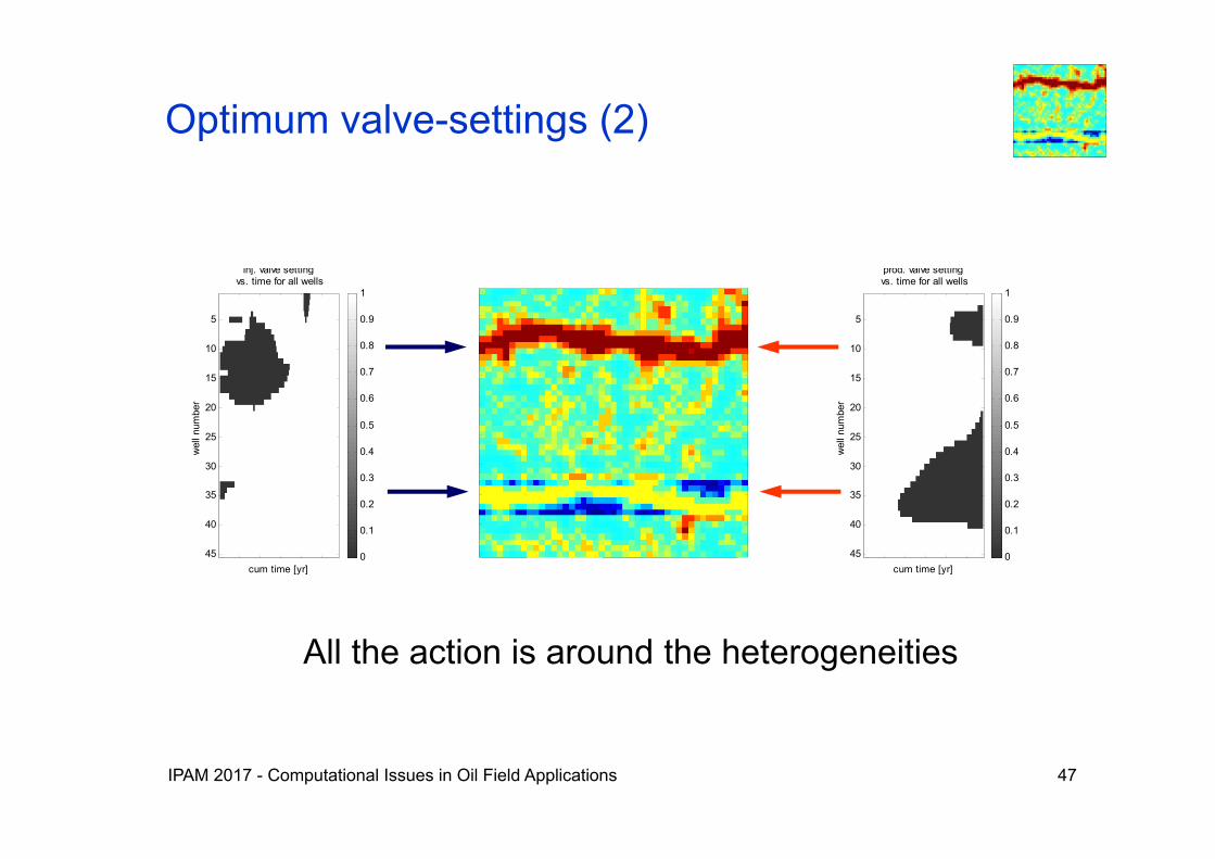
Optimum valve-settings (2)
0
0.1
0.2
0.3
0.4
0.5
0.6
0.7
0.8
0.9
1
cum time [yr]
wel
l num
ber
inj. valve setting vs. time for all wells
5
10
15
20
25
30
35
40
45 0
0.1
0.2
0.3
0.4
0.5
0.6
0.7
0.8
0.9
1
cum time [yr]
wel
l num
ber
prod. valve setting vs. time for all wells
5
10
15
20
25
30
35
40
450
0.1
0.2
0.3
0.4
0.5
0.6
0.7
0.8
0.9
1
cum time [yr]
wel
l num
ber
inj. valve setting vs. time for all wells
5
10
15
20
25
30
35
40
45 0
0.1
0.2
0.3
0.4
0.5
0.6
0.7
0.8
0.9
1
cum time [yr]
wel
l num
ber
prod. valve setting vs. time for all wells
5
10
15
20
25
30
35
40
45
All the action is around the heterogeneities
IPAM 2017 - Computational Issues in Oil Field Applications 48
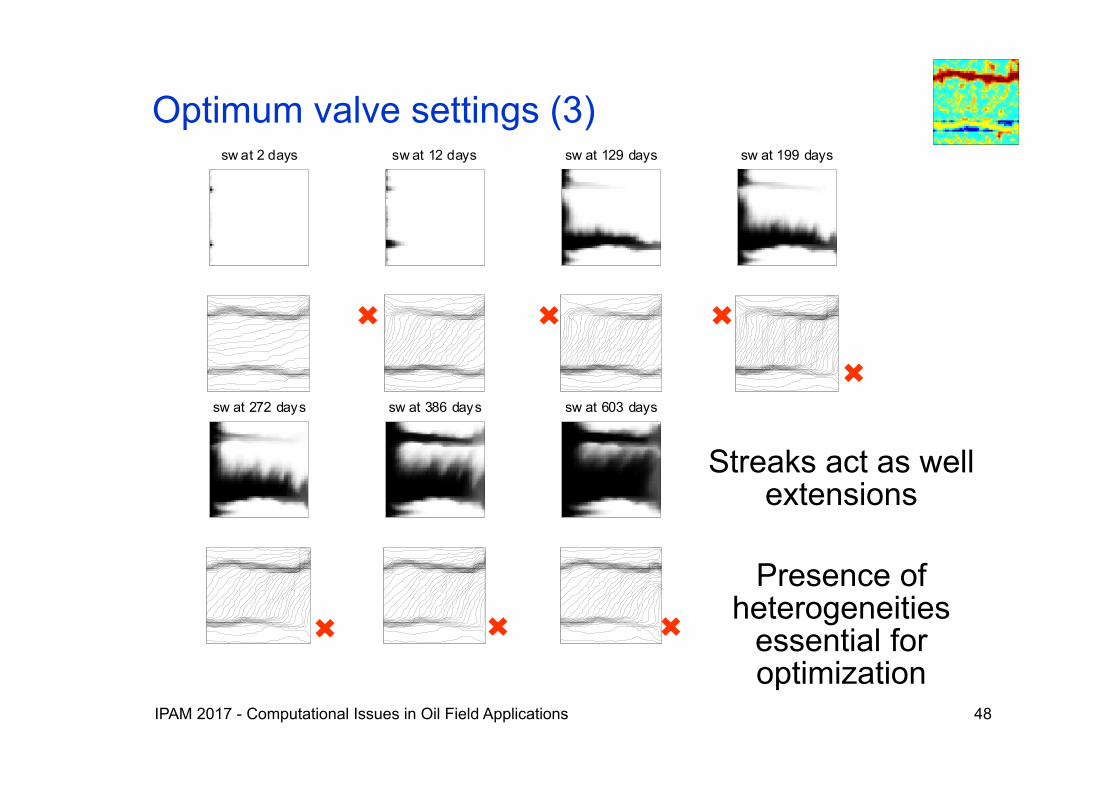
sw at 2 days sw at 12 days sw at 129 days sw at 199 days
sw at 272 days sw at 386 days sw at 603 days
Optimum valve settings (3)
Streaks act as well extensions
Presence of heterogeneities
essential for optimization
IPAM 2017 - Computational Issues in Oil Field Applications 49
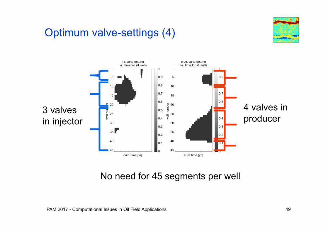
Optimum valve-settings (4)
0
0.1
0.2
0.3
0.4
0.5
0.6
0.7
0.8
0.9
1
cum time [yr]
wel
l num
ber
inj. valve setting vs. time for all wells
5
10
15
20
25
30
35
40
45 0
0.1
0.2
0.3
0.4
0.5
0.6
0.7
0.8
0.9
1
cum time [yr]
wel
l num
ber
prod. valve setting vs. time for all wells
5
10
15
20
25
30
35
40
45
3 valves in injector
4 valves in producer
No need for 45 segments per well
IPAM 2017 - Computational Issues in Oil Field Applications 50
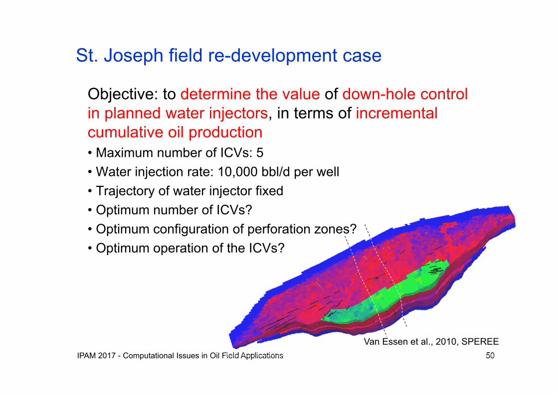
St. Joseph field re-development case
Objective: to determine the value of down-hole control in planned water injectors, in terms of incremental cumulative oil production• Maximum number of ICVs: 5• Water injection rate: 10,000 bbl/d per well• Trajectory of water injector fixed• Optimum number of ICVs?• Optimum configuration of perforation zones? • Optimum operation of the ICVs?
Van Essen et al., 2010, SPEREE

IPAM 2017 - Computational Issues in Oil Field Applications 51
Pilot study on sector model
• Strongly layered structure • Very limited vertical communication• Dips approximately 20º• 21,909 active grid blocks• Dimensions 1600m x 500m x 450m• No aquifer support• 1 gas injection well• 1 (planned) water injection well• 7 production wells in sector
IPAM 2017 - Computational Issues in Oil Field Applications 52
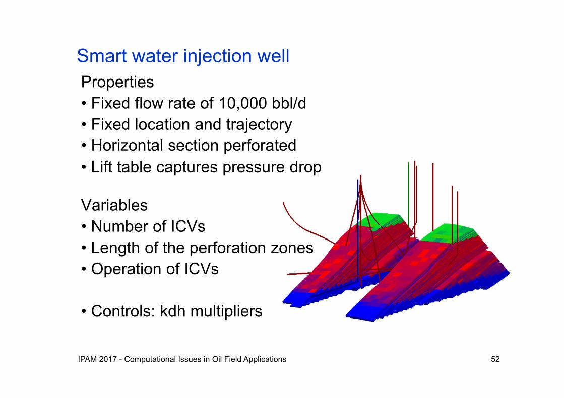
Smart water injection wellProperties• Fixed flow rate of 10,000 bbl/d• Fixed location and trajectory• Horizontal section perforated• Lift table captures pressure drop
Variables• Number of ICVs• Length of the perforation zones• Operation of ICVs
• Controls: kdh multipliers
IPAM 2017 - Computational Issues in Oil Field Applications 53
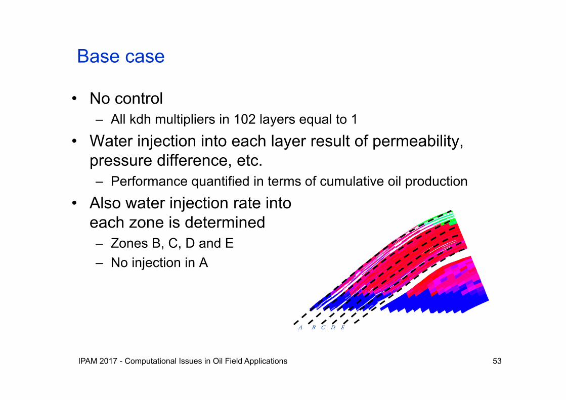
Base case
• No control– All kdh multipliers in 102 layers equal to 1
• Water injection into each layer result of permeability, pressure difference, etc.– Performance quantified in terms of cumulative oil production
• Also water injection rate intoeach zone is determined– Zones B, C, D and E– No injection in A
A B C D E

IPAM 2017 - Computational Issues in Oil Field Applications 54
Base case results
• Cumulative oil production: 11.47 MMstb
2010 2012 2014 2016 2018 20200
5
10
15x 106
Vol
ume
[stb
]
Cumulative production data
oil productionwater production
2010 2012 2014 2016 2018 20200
2000
4000
6000
8000
10000
Rat
e [s
tb/d
ay]
Injection per group
Group BGroup CGroup DGroup E
Van Essen et al., 2010, SPEREE
IPAM 2017 - Computational Issues in Oil Field Applications 55
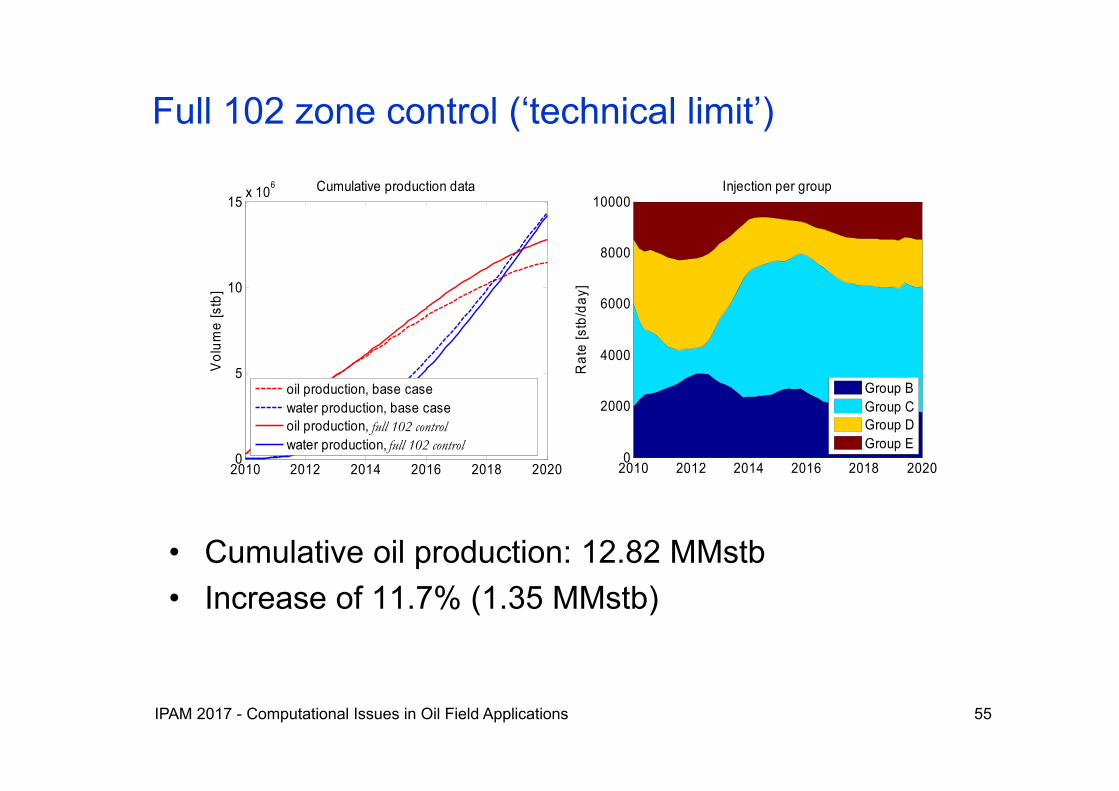
Full 102 zone control (‘technical limit’)
• Cumulative oil production: 12.82 MMstb• Increase of 11.7% (1.35 MMstb)
2010 2012 2014 2016 2018 20200
5
10
15x 106
Vol
ume
[stb
]
Cumulative production data
oil production, base casewater production, base caseoil production, standard 4-group controlwater production, standard 4-group control
2010 2012 2014 2016 2018 20200
2000
4000
6000
8000
10000
Rat
e [s
tb/d
ay]
Injection per group
Group BGroup CGroup DGroup E
full 102 controlfull 102 control

IPAM 2017 - Computational Issues in Oil Field Applications 56
Standard 4-group control (geological insight)
• Cumulative oil production: 12.40 MMstb• Increase of 8.1% (0.93 MMstb)
2010 2012 2014 2016 2018 20200
5
10
15x 106
Vol
ume
[stb
]
Cumulative production data
oil production, base casewater production, base caseoil production, standard 4-group controlwater production, standard 4-group control
2010 2012 2014 2016 2018 20200
2000
4000
6000
8000
10000
Rat
e [s
tb/d
ay]
Injection per group
Group BGroup CGroup DGroup E

IPAM 2017 - Computational Issues in Oil Field Applications 57
Alternative 4-group control (optimal grouping)
• Cumulative oil production: 12.62 MMstb• Increase of 10.0% (1.15 MMstb)
2010 2012 2014 2016 2018 20200
5
10
15x 106
Vol
ume
[stb
]
Cumulative production data
oil production, base casewater production, base caseoil production, alternative 4-group controlwater production, alternative 4-group control
2010 2012 2014 2016 2018 20200
2000
4000
6000
8000
10000
Rat
e [s
tb/d
ay]
Injection per group
Group B*Group C*Group D*Group E*
IPAM 2017 - Computational Issues in Oil Field Applications 58
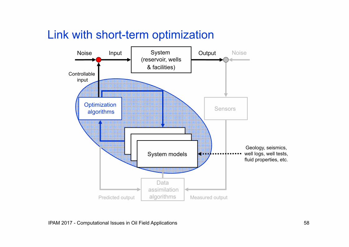
Dataassimilationalgorithms
Noise OutputInput NoiseSystem (reservoir, wells
& facilities)
Optimizationalgorithms Sensors
System models
Predicted output Measured output
Controllableinput
Geology, seismics,well logs, well tests,fluid properties, etc.
Link with short-term optimization

IPAM 2017 - Computational Issues in Oil Field Applications 59
Life-cycle optimization vs. reactive control (1)
IPAM 2017 - Computational Issues in Oil Field Applications 60
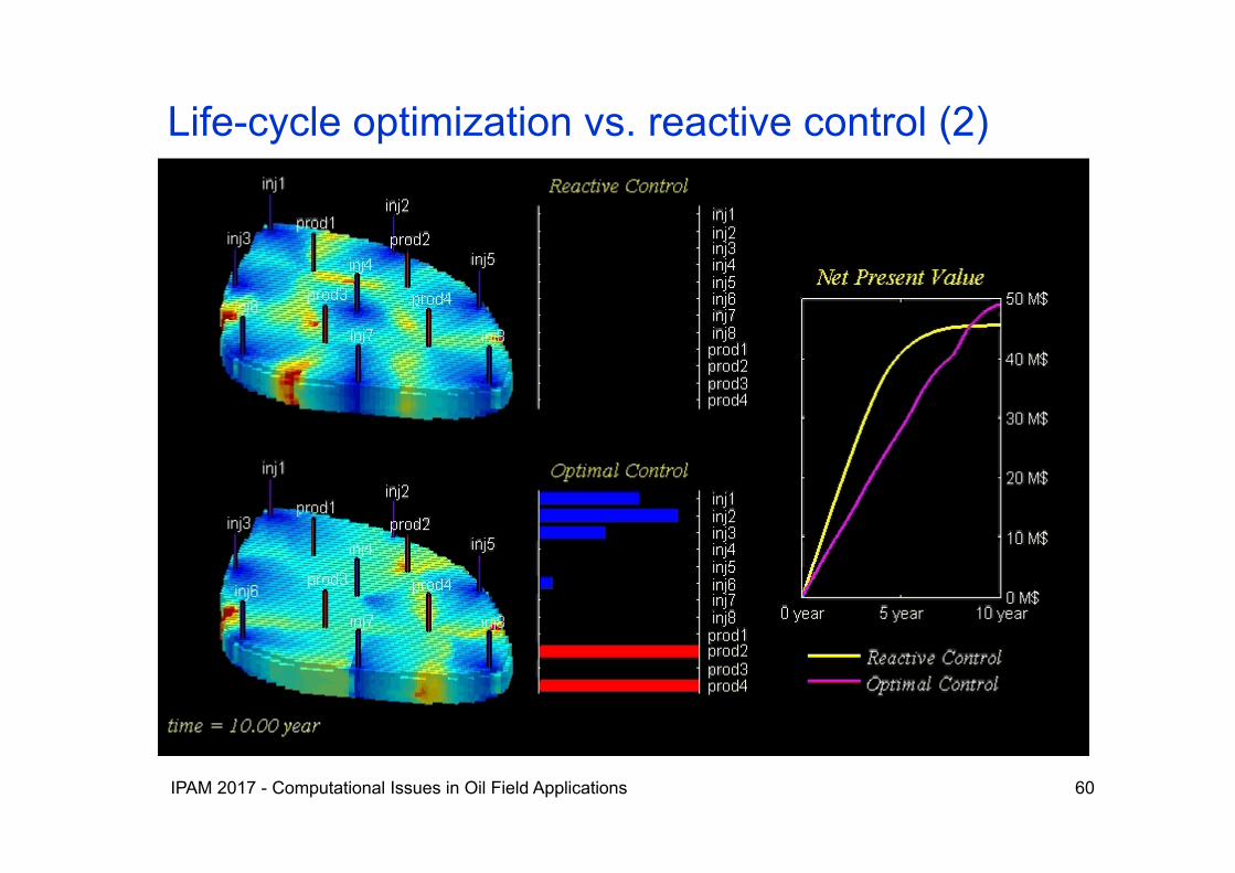
Life-cycle optimization vs. reactive control (2)
IPAM 2017 - Computational Issues in Oil Field Applications 61
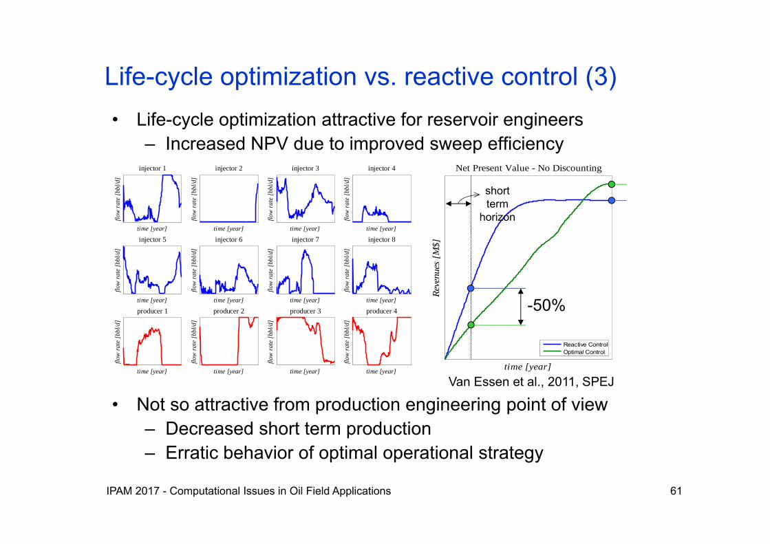
• Life-cycle optimization attractive for reservoir engineers– Increased NPV due to improved sweep efficiency
• Not so attractive from production engineering point of view– Decreased short term production– Erratic behavior of optimal operational strategy
Net Present Value - No Discounting
time [year]
Reve
nues
[M
$]
Reactive ControlOptimal Control
injector 1
time [year]
flow
rat
e [b
bl/d
]
injector 2
time [year]
flow
rat
e [b
bl/d
]
injector 3
time [year]
flow
rat
e [b
bl/d
]
injector 4
time [year]
flow
rat
e [b
bl/d
]
injector 5
time [year]
flow
rat
e [b
bl/d
]
injector 6
time [year]
flow
rat
e [b
bl/d
]
injector 7
time [year]
flow
rat
e [b
bl/d
]
injector 8
time [year]
flow
rat
e [b
bl/d
]
producer 1
time [year]
flow
rat
e [b
bl/d
]
producer 2
time [year]
flow
rat
e [b
bl/d
]
producer 3
time [year]
flow
rat
e [b
bl/d
]
producer 4
time [year]
flow
rat
e [b
bl/d
]
+10%
-50%
short term
horizon
Life-cycle optimization vs. reactive control (3)
Van Essen et al., 2011, SPEJ

IPAM 2017 - Computational Issues in Oil Field Applications 62
• Take production objectives into account by incorporating them as additional optimization criteria:
• Formal solution:– Order objectives according to importance– Optimize objectives sequentially– Optimality of upper objective constrains optimization of
lower one
• Only possible if there are redundant degrees of freedom in input parameters after meeting primary objective
Hierarchical optimization
IPAM 2017 - Computational Issues in Oil Field Applications 63
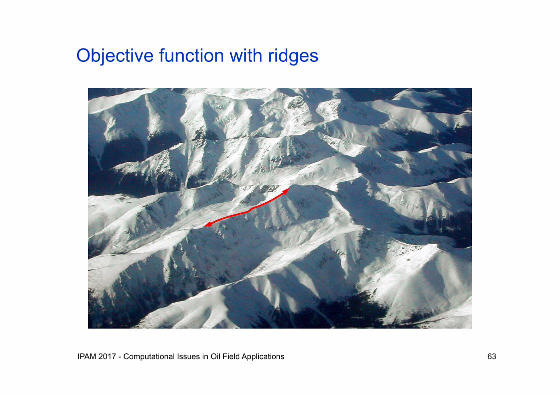
Objective function with ridges

IPAM 2017 - Computational Issues in Oil Field Applications 64
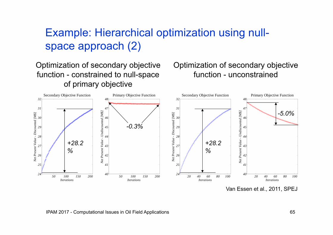
• 3D reservoir• 8 injection / 4 production wells• Period of 10 years • Producers at constant BHP• Rates in injectors optimized
• Primary objective: undiscountedNPV over the life of the field •Secondary objective: NPV with very high discount factor(25%) to emphasize importance of short term production
Example: Hierarchical optimization using null-space approach (1)
IPAM 2017 - Computational Issues in Oil Field Applications 65
20 40 60 80 10024
25
26
27
28
29
30
31
32
Iterations
Net P
rese
nt V
alue
- D
iscou
nted
[M$]
Secondary Objective Function
20 40 60 80 10040
41
42
43
44
45
46
47
48
Iterations
Net
Pre
sent
Val
ue -
Und
iscou
nted
[M$]
Primary Objective Function
50 100 150 20024
25
26
27
28
29
30
31
32
Iterations
Net P
rese
nt V
alue
- D
iscou
nted
[M$]
Secondary Objective Function
50 100 150 20040
41
42
43
44
45
46
47
48
Iterations
Net
Pre
sent
Val
ue -
Und
iscou
nted
[M$]
Primary Objective Function
Optimization of secondary objective function - constrained to null-space
of primary objective
Optimization of secondary objective function - unconstrained
+28.2%
+28.2%
-0.3%
-5.0%
Example: Hierarchical optimization using null-space approach (2)
Van Essen et al., 2011, SPEJ
IPAM 2017 - Computational Issues in Oil Field Applications 66
0 900 1800 2700 36000
5
10
15
20
25
30
35
40
45
50
time [days]
NPV
ove
r Ti
me
- Und
isco
unte
d [1
0 6 $
]
~~
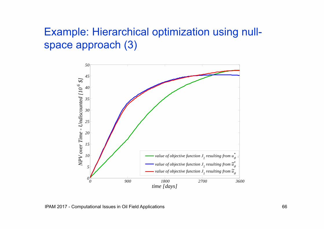
value of objective function J1 resulting from u* .
value of objective function J1 resulting from u*
value of objective function J1 resulting from u
Example: Hierarchical optimization using null-space approach (3)

IPAM 2017 - Computational Issues in Oil Field Applications 67
Controlability of a dynamic system is the ability to influence the states through manipulation of the inputs.
Observability of a dynamic system is the ability to determine the states through observation of the outputs.
Identifiability of a dynamic system is the ability to determine the parameters from the input-output behavior.
All very limited for reservoir simulation models!Zandvliet, M. et al., 2008: Computational Geosciences 12 (4) 808-822.
Van Doren, J.F.M., et al. 2013: Computational Geosciences 17 (5) 773-788.
System model
state (p,S)parameters (k,φ,…)
output (pwf ,qw ,qo)input (pwf ,qt)
Observability, controlability, identifiability
IPAM 2017 - Computational Issues in Oil Field Applications 68
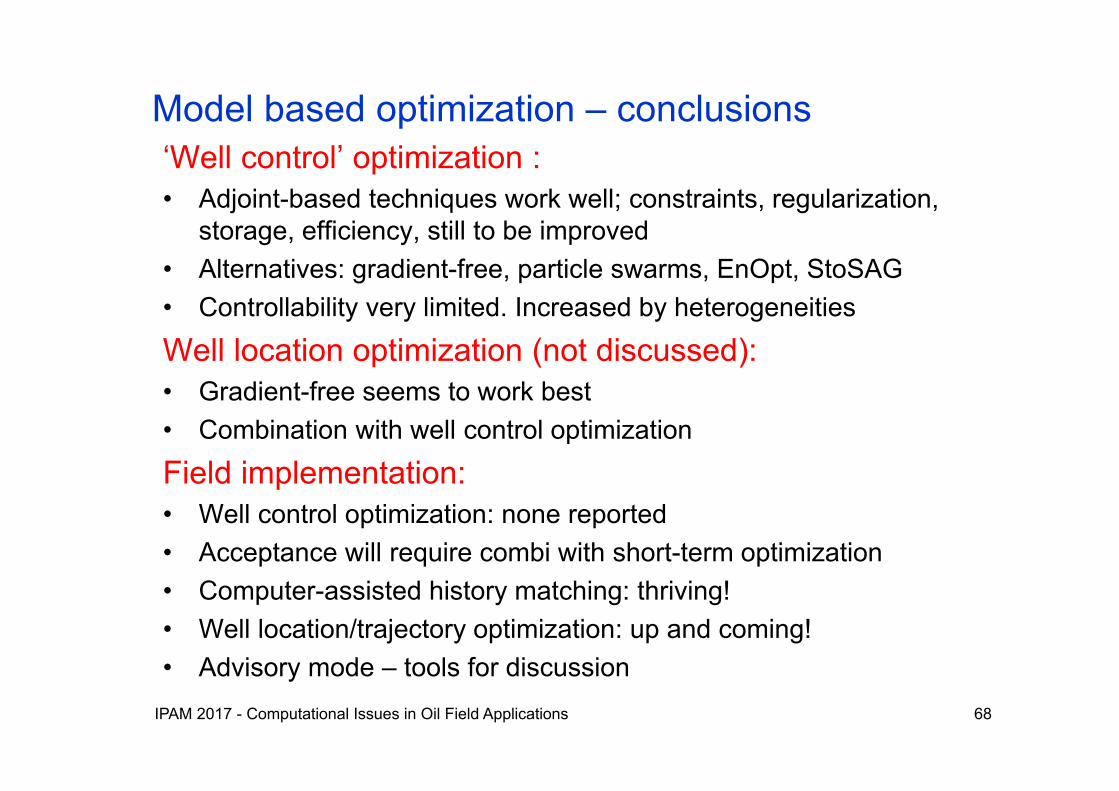
Model based optimization – conclusions‘Well control’ optimization :• Adjoint-based techniques work well; constraints, regularization,
storage, efficiency, still to be improved• Alternatives: gradient-free, particle swarms, EnOpt, StoSAG• Controllability very limited. Increased by heterogeneities
Well location optimization (not discussed):• Gradient-free seems to work best• Combination with well control optimization
Field implementation:• Well control optimization: none reported• Acceptance will require combi with short-term optimization• Computer-assisted history matching: thriving!• Well location/trajectory optimization: up and coming!• Advisory mode – tools for discussion
IPAM 2017 - Computational Issues in Oil Field Applications 69
References adjoint-based optimization (1)Review paper (with additional references)Jansen, J.D., 2011: Adjoint-based optimization of multiphase flow through porous media –a review. Computers and Fluids 46 (1) 40-51. DOI: 10.1016/j.compfluid.2010.09.039.Early use in history matchingChavent, G., Dupuy, M. and Lemonnier, P., 1975: History matching by use of optimal theory. SPE Journal 15 (1) 74-86. DOI: 10.2118/4627-PA.Chen, W.H., Gavalas, G.R. and Wasserman, M.L., 1974: A new algorithm for automatic history matching. SPE Journal 14 (6) 593-608. DOI: 10.2118/4545-PA. Li, R., Reynolds, A.C., and Oliver, D.S., 2003: History matching of three-phase flow production data. SPE Journal 8 (4): 328-340. DOI: 10.2118/87336-PA.Early use in flooding optimizationRamirez, W.F., 1987: Application of optimal control theory to enhanced oil recovery, Elsevier, Amsterdam.Asheim, H., 1988: Maximization of water sweep efficiency by controlling production and injection rates. Paper SPE 18365 presented at the SPE European Petroleum Conference, London, UK, October 16-18. DOI: 10.2118/18365-MS.Virnovski, G.A., 1991: Water flooding strategy design using optimal control theory, Proc.6th European Symposium on IOR, Stavanger, Norway, 437-446.

IPAM 2017 - Computational Issues in Oil Field Applications 70
References adjoint-based optimization (2)Zakirov, I.S., Aanonsen, S.I., Zakirov, E.S., and Palatnik, B.M., 1996: Optimization of reservoir performance by automatic allocation of well rates. Proc. 5th European Conference on the Mathematics of Oil Recovery (ECMOR V), Leoben, Austria.Sudaryanto, B. and Yortsos, Y.C., 2000: Optimization of fluid front dynamics in porous media using rate control. Physics of Fluids 12 (7) 1656-1670. DOI: 10.1063/1.870417.TU Delft seriesBrouwer, D.R. and Jansen, J.D., 2004: Dynamic optimization of water flooding with smart wells using optimal control theory. SPE Journal 9 (4) 391-402. DOI: 10.2118/78278-PA.Van Doren, J.F.M., Markovinović, R. and Jansen, J.D., 2006: Reduced-order optimal control of waterflooding using POD. Computational Geosciences 10 (1) 137-158. DOI: 10.1007/s10596-005-9014-2.Zandvliet, M.J., Bosgra, O.H., Van den Hof, P.M.J., Jansen, J.D. and Kraaijevanger, J.F.B.M., 2007: Bang-bang control and singular arcs in reservoir flooding. Journal of Petroleum Science and Engineering 58, 186-200. DOI: 10.1016/j.petrol.2006.12.008.Lien, M., Brouwer, D.R., Manseth, T. and Jansen, J.D., 2008: Multiscale regularization of flooding optimization for smart field management. SPE Journal 13 (2) 195-204. DOI: 10.2118/99728-PA.Zandvliet, M.J., Handels, M., Van Essen, G.M., Brouwer, D.R. and Jansen, J.D., 2008: Adjoint-based well placement optimization under production constraints. SPE Journal 13(4) 392-399. DOI: 10.2118/105797-PA.
IPAM 2017 - Computational Issues in Oil Field Applications 71
References adjoint-based optimization (3)Van Essen, G.M., Zandvliet, M.J., Van den Hof, P.M.J., Bosgra, O.H. and Jansen, J.D., 2009: Robust waterflooding optimization of multiple geological scenarios. SPE Journal 14(1) 202-210. DOI: 10.2118/102913-PA.Van Essen, G.M., Jansen, J.D., Brouwer, D.R. Douma, S.G., Zandvliet, M.J., Rollett, K.I. and Harris, D.P., 2010: Optimization of smart wells in the St. Joseph field. SPE Reservoir Evaluation and Engineering 13 (4) 588-595. DOI: 10.2118/123563-PA. Van Essen, G.M., Van den Hof, P.M.J. and Jansen, J.D., 2011: Hierarchical long-term and short-term production optimization. SPE Journal 16 (1) 191-199. DOI: 10.2118/124332-PA.Farshbaf Zinati, F., Jansen, J.D. and Luthi, S.M., 2012: Estimating the specific productivity index in horizontal wells from distributed pressure measurements using an adjoint-based minimization algorithm. SPE Journal 17 (3) 742-751. DOI: 10.2118/135223-PA.Namdar Zanganeh, M., Kraaijevanger, J.F.B.M., Buurman, H.W., Jansen, J.D., Rossen, W.R., 2014: Challenges in adjoint-based optimization of a foam EOR process. Computational Geosciences 18 (3-4) 563–577. DOI: 10.1007/s10596-014-9412-4.de Moraes R.J., Rodrigues, J.R.P., Hajibeygi, H. and Jansen, J.D., 2017: Multiscale gradient computation for subsurface flow models. Journal of Computational Physics. Published online. DOI: 10.1016/j.jcp.2017.02.024.
IPAM 2017 - Computational Issues in Oil Field Applications 72
References adjoint-based optimization (4)Computational aspectsSarma, P., Aziz, K. and Durlofsky, L.J., 2005: Implementation of adjoint solution for optimal control of smart wells. Paper SPE 92864 presented at the SPE Reservoir Simulation Symposium, Houston, USA, 31 January – 2 February. DOI: 10.2118/92864-MS.Han, C., Wallis, J., Sarma, P. et al., 2013: Adaptation of the CPR preconditioner for efficient solution of the adjoint equation. SPE Journal 18 (2) 207-213. DOI: org/10.2118/141300-PA.Algebraic formulationRodrigues, J.R.P., 2006: Calculating derivatives for automatic history matching. Computational Geosciences 10 (1) 119-136. DOI: 10.1007/s10596-005-9013-3.Kraaijevanger, J.F.B.M., Egberts, P.J.P., Valstar, J.R. and Buurman, H.W., 2007: Optimal waterflood design using the adjoint method. Paper SPE 105764 presented at the SPE Reservoir Simulation Symposium, Houston, USA, 26-28 February. DOI: 10.2118/105764-MS.Constraint handlingDe Montleau, P., Cominelli, A., Neylon, K. and Rowan, D., Pallister, I., Tesaker, O. and Nygard, I., 2006: Production optimization under constraints using adjoint gradients. Proc. 10th European Conference on the Mathematics of Oil Recovery (ECMOR X), Paper A041, Amsterdam, The Netherlands, September 4-7.
IPAM 2017 - Computational Issues in Oil Field Applications 73
References adjoint-based optimization (5)Sarma, P., Chen, W.H. Durlofsky, L.J. and Aziz, K., 2008: Production optimization with adjoint models under nonlinear control-state path inequality constraints. SPE Reservoir Evaluation and Engineering 11 (2) 326-339. DOI: 10.2118/99959-PA.Suwartadi, E., Krogstad, S. & Foss, B., 2012: Nonlinear output constraints handling for production optimization of oil reservoirs. Computational Geosciences 16 (2) 499–517. DOI 10.1007/s10596-011-9253-3.Kourounis, D., Durlofsky, L.J., Jansen, J.D. and Aziz, K., 2014: Adjoint formulation and constraint handling for gradient-based optimization of compositional reservoir flow. Computational Geosciences 18 (2) 117-137. DOI: 10.1007/s10596-013-9385-8.Kourounis, D. and Schenk, O., 2015: Constraint handling for gradient-based optimization of compositional reservoir flow. Computational Geosciences 19 1109-1122. DOI:10.1007/s10596-015-9524-5. Closed-loop reservoir managementJansen, J.D., Brouwer, D.R., Nævdal, G. and van Kruijsdijk, C.P.J.W., 2005: Closed-loop reservoir management. First Break, January, 23, 43-48.Naevdal, G., Brouwer, D.R. and Jansen, J.D., 2006: Waterflooding using closed-loop control. Computational Geosciences 10 (1) 37-60. DOI: 10.1007/s10596-005-9010-6.Sarma, P., Durlofsky, L.J., Aziz, K., Chen, W.H., 2006: Efficient real-time reservoir management using adjoint-based optimal control and model updating. Computational Geosciences 10 (1) 3-36. DOI: 10.1007/s10596-005-9009-z.

IPAM 2017 - Computational Issues in Oil Field Applications 74
References adjoint-based optimization (6)Jansen, J.D., Bosgra, O.H. and van den Hof, P.M.J., 2008: Model-based control of multiphase flow in subsurface oil reservoirs. Journal of Process Control 18, 846-855. DOI: 10.1016/j.jprocont.2008.06.011.Sarma, P., Durlofsky, L.J. and Aziz, K., 2008: Computational techniques for closed-loop reservoir modeling with application to a realistic reservoir. Petroleum Science and Technology 26 (10 & 11) 1120-1140. DOI: 10.1080/10916460701829580.Jansen, J.D., Douma, S.G., Brouwer, D.R., Van den Hof, P.M.J., Bosgra, O.H. and Heemink, A.W., 2009: Closed-loop reservoir management. Paper SPE 119098 presented at the SPE Reservoir Simulation Symposium, The Woodlands, USA, 2-4 February. DOI: 10.2118/119098-MS.Wang, C., Li, G. and Reynolds, A.C., 2009: Production optimization in closed-loop reservoir management. SPE Journal 14 (3) 506-523. DOI: 10.2118/109805-PA.Foss, B. and Jensen, J.P., 2010: Performance analysis for closed-loop reservoir management. SPE Journal 16 (1) 183-190. DOI: 10.2118/138891-PA.Chen, C., Li, G. and Reynolds, A.C., 2012: Robust constrained optimization of short- and long-term net present value for closed-loop reservoir management. SPE Journal 17 (3) 849-864. DOI: 10.2118/141314-PA.Bukshtynov, V., Volkov, O., Durlofsky, L.J. and Aziz, K., 2015: Comprehensive framework for gradient-based optimization in closed-loop reservoir management. Computational Geosciences 19 (4) 877-897. DOI:10.1007/s10596-015-9496-5.

IPAM 2017 - Computational Issues in Oil Field Applications 75
Acknowledgments
• Colleagues and students of– TU Delft – Department of Geoscience and Engineering– TU Eindhoven (TUE) – Department of Electrical Engineering– TU Delft – Delft Institute for Applied Mathematics– TNO – Built Environment and Geosciences
• Especially for the optimization results presented in this tutorial:Prof. Paul Van den Hof (TUE), Prof. Arnold Heemink (TUD), and (former) PhD students Roald Brouwer, Maarten Zandvliet andGijs van Essen
• Sponsors: Shell (Recovery Factory program),ENI, Petrobras, Statoil (ISAPP program)