DELFT UNIVERSITY OF TECHNOLOGY

REPORT 06-07

Numerical Methods for CVD Simulation

S. van Veldhuizen, C. Vuik, C.R. Kleijn

ISSN 1389-6520

Reports of the Department of Applied Mathematical Analysis

Delft 2006

Copyright 2006 by Delft Institute of Applied Mathematics Delft, The Netherlands.

No part of the Journal may be reproduced, stored in a retrieval system, or transmitted, inany form or by any means, electronic, mechanical, photocopying, recording, or otherwise,without the prior written permission from Delft Institute of Applied Mathematics, DelftUniversity of Technology, The Netherlands.

Numerical Methods for CVD Simulation

S. van Veldhuizen∗ C. Vuik∗ C.R. Kleijn†

May 8, 2006

Abstract

In this study various numerical schemes for simulating 2D laminar reacting gasflows, as typically found in Chemical Vapor Deposition (CVD) reactors, are proposedand compared. These systems are generally modeled by means of many stiffly coupledelementary gas phase reactions between a large number of reactants and intermediatespecies. The purpose of this study is to develop robust and efficient solvers forthe stiff heat-reaction system, whereby the velocities are assumed to be given. Fornon-stationary CVD simulation, an optimal combination in terms of efficiency androbustness between time integration, nonlinear solvers and linear solvers has to befound. Besides stability, which is important due to the stiffness of the problem,the preservation of non-negativity of the species is crucial. It appears that this extracondition on time integration methods is much more restrictive towards the time-stepthan stability. For a set of suitable time integration methods necessary conditions arerepresented. We conclude with a comparison of the workload between the selectedtime integration methods. This comparison has been done for a 2D test problem.The test problem does not represent a practical process, but represents only thecomputational problems.

1 Introduction

Chemical Vapor Deposition (CVD) is a process that synthesizes a thin solid film fromthe gaseous phase by a chemical reaction on a solid material. Applications of thin solidfilms as, for instance, insulating and (semi) conducting layers, can be found in manytechnological areas such as micro-electronics, optical devices and so on.

A CVD system is a chemical reactor, wherein the material to be deposited is injectedas a gas and which contains the substrates on which deposition takes place. The energy todrive the chemical reaction is (usually) thermal energy. On the substrates surface reactionswill take place resulting in deposition of a thin film.

∗Delft University of Technology, Delft Institute of Applied Mathematics, Mekelweg 4, 2628 CD Delft,The Netherlands (s.vanveldhuizen@tudelft.nl, c.vuik@tudelft.nl)

†Delft University of Technology, Department of Multi Scale Physics, Prins Bernardlaan 6, 2628 BWDelft, The Netherlands (c.r.kleijn@tudelft.nl)

1

In CVD literature, and also other reactive flow literature, one is usually looking forthe steady state solution of the so-called species equations (6). The species equationsdescribe the transport of mass due to advective and diffusive transport, and due to thechemical reactions in the reactor. The usual procedure to find this steady state solutionis to perform a (damped/relaxed) Newton iteration with an (arbitrary) initial solution.Hopefully, the Newton iteration then converges to the steady state. If this is not the caseone performs some (artificial) time stepping in order to find a better initial solution forthe next Newton iteration. In this paper we present suitable time integration methods forstiff problems. Furthermore, we compare these integration methods by their performance,in terms of efficiency.

In our research we are not looking for the steady state solution only, but we also wantto approximate the transient solution. Since the time scales of advection and diffusiondiffer orders of magnitude from the time scales of the chemical reactions the system ofspecies equations becomes stiff. Thus, in order to integrate the species equations in time ina stable manner, time integration methods have to be found that can handle stiff systems.Besides the stability issue for time integration, also the preservation of non-negativity ofthe species during time integration is important. It appears that this last condition ontime integration methods is much more restrictive towards the time step than stability.

In this report issues on stability of time integration methods are discussed, as wellas the positivity properties, see Section 3 and 4. The next step is to make a selection ofsuitable time integration methods, which will be presented in Section 5. This report will beconcluded with numerical results, Section 6, obtained with the representative test problemproposed in Section 2.

2 Model for CVD Simulation

The mathematical model describing the CVD process consists of a set of partial dif-ferential equations with appropriate boundary conditions, which describe the gas flow, thetransport of energy, the transport of species and the chemical reactions in the reactor.

The gas mixture in the reactor is assumed to behave as a continuum. This assumptionis only valid when the mean free path of the molecules is much smaller than a characteristicdimension of the reactor. For Knudsen numbers Kn < 0.01, where

Kn =ξ

L, (1)

the gas mixture behaves as a continuum. In (1) ξ is the mean free path length of themolecules and L a typical characteristic dimension of the reactor. For pressures largerthan 100 Pa and typical reactor dimensions larger than 0.01 m the continuum approachcan be used safely. See, for example, [9].

Furthermore, the gas mixture is assumed to behave as an ideal and transparent gas1

behaving in accordance with Newton’s law of viscosity. The gas flow in the reactor is

1By transparent we mean that the adsorption of heat radiation by the gas(es) will be small.

2

assumed to be laminar (low Reynolds number flow). Since no large velocity gradientsappear in CVD gas flows, viscous heating due to dissipation will be neglected. We alsoneglect the effects of pressure variations in the energy equation.

The composition of the N component gas mixture is described in terms of the dimen-sionless mass fractions ωi = ρi

ρ, i = 1, . . . , N , having the property

N∑

i=1

ωi = 1. (2)

The transport of mass, momentum and heat are described respectively by the continuityequation (3), the Navier-Stokes equations (4) and the transport equation for thermal energy(5) expressed in terms of temperature T :

∂ρ

∂t= −∇ · (ρv), (3)

∂(ρv)

∂t= −(∇ρv) · v + ∇ ·

[

µ(

∇v + (∇v)T)

− 2

3µ(∇ · v)I

]

−∇P + ρg, (4)

cp∂(ρT )

∂t= −cp∇ · (ρvT ) + ∇ · (λ∇T ) +

+∇ ·(

RT

N∑

i=1

DTi

Mi

∇fi

fi

)

+

N∑

i=1

Hi

mi∇ · ji

−N∑

i=1

K∑

k=1

HiνikRgk, (5)

with ρ gas mixture density, v mass averaged velocity vector, µ the viscosity, I the unittensor, g gravity acceleration,cp specific heat ( J

mol·K), λ the thermal conductivity ( W

m·K)

and R the gas constant. Gas species i has a mole fraction fi, a molar mass mi, a thermaldiffusion coefficient DT

i , a molar enthalpy Hi and a diffusive mass flux ji. The stoichiometriccoefficient of the ith species in the kth gas-phase reaction with net molar reaction rate Rg

k

is νik.We assume that in the gas-phase K reversible reactions take place. For the kth reaction

the net molar reaction rate is denoted as Rgk

(

molem3·s

)

. For an explicit description of thenet molar reaction rate, we refer to [9, 16]. The balance equation for the ith gas species,i = 1, . . . , N , in terms of mass fractions and diffusive mass fluxes is then given as

∂(ρωi)

∂t= −∇ · (ρvωi) −∇ · ji + mi

K∑

k=1

νikRgk, (6)

where ji is the diffusive flux. This mass diffusion flux is decomposed into concentrationdiffusion and thermal diffusion, e.g.,

ji = jCi + jTi . (7)

3

The first type of diffusion, jCi , occurs as a result of a concentration gradient in the system.Thermal diffusion is the kind of diffusion resulting from a temperature gradient. For amulticomponent gas mixture there are two approaches for the treatment of the ordinarydiffusion, namely the full Stefan-Maxwell equations and an alternative approximation de-rived by Wilke. In this case, we have chosen for Wilke’s approach. Then, the speciesconcentration equations become

∂(ρωi)

∂t= −∇ · (ρvωi) + ∇ · (ρD

′i∇ωi) + ∇ · (DT

i ∇(ln T )) +

+mi

K∑

k=1

νikRgk, (8)

where D′i is an effective diffusion coefficient for species i and DT

i the multi-componentthermal diffusion coefficient for species i.

The main focus of our research is on efficient solvers for the above species equation(s)(8). Typically the time scales of the slow and fast reaction terms differ orders of magnitudefrom each other and from the time scales of the diffusion and advection terms, leading toextremely stiff systems.

2.1 Simplified CVD System

Since our research focuses on solving the species equations (8), we will only solve thecoupled system of N species equations, where N denotes the number of gas-species in thereactor. Note that it suffices to solve the N − 1 coupled species equations for all speciesexcept the carrier gas, where its mass fraction ωHe will be computed via the property

N∑

i=1

ωi = 1. (9)

For the moment we only focus on the development of efficient solvers for species equa-tions. Therefore, we will omit the surface reactions in our system, because these boundaryconditions will need some extra attention. Another simplification is that we assume thatboth the velocity field, temperature field, pressure field and density field are given. To bemore precise, they are computed via another simulation package which was developed byKleijn [10]. Furthermore, we omit thermal diffusion.

2.2 Reactor Geometry

The studied reactor configuration is illustrated in Figure 1. As computational domainwe take, because of axisymmetry, one half of the r − z plane.

The pressure in the reactor is 1 atm. From the top a gas-mixture, consisting of silaneand helium, enters the reactor with a uniform temperature Tin = 300 K and a uniformvelocity uin. The inlet silane mole fraction is fin,SiH4

= 0.001, whereas the rest is helium.

4

r

z

θ

susceptor

outflow

inflow

solidwall

dT/dr = 0v = 0u = 0

T=300 K f_SiH4= 0.001 f_He= 0.999 v= 0.10 m/s

T=1000 K u, v = 0

dT/dz = 0

dv/dz = 0

0.175 m

0.15 m0.

10 m

Figure 1: Reactor geometry

5

At a distance of 10 cm. below the inlet a susceptor with temperature T = 1000 K and adiameter 30 cm. is placed. As mentioned before, on this surface no reactions (will) takeplace. Unlike the problem considered in [10] the susceptor does not rotate.

2.3 Gas-Phase Reaction Model

We consider a CVD process that deposits solid silicon Si from gaseous silane SiH4. InCVD literature one usually considers gas phase chemistry models consisting of 16 - 50species. In our simplified CVD system we consider a gas mixture consisting of 7 species.Besides the carrier gas helium and the reactive specie silane, the mixture contains

• silane SiH4,

• helium He,

• silylane SiH2,

• H2SiSiH2,

• disilane Si2H6,

• trisilane Si3H8, and

• hydrogen H2.

The reactive species in the gas mixture satisfy the reaction mechanism

G1 : SiH4 SiH2 + H4

G2 : Si2H6 SiH4 + SiH2

G3 : Si2H6 H2SiSiH2 + H2

G4 : SiH2+Si2H6 Si3H8

G5 : 2Si2 H2SiSiH2

As can be found in [16], the forward reaction rate kforward is fitted according to the modifiedLaw of Arrhenius as

kgforward(T ) = AkT

βke−EkRT . (10)

The backward reaction rates are self consistent with

kgbackward(T ) =

kgforward(T )

Kg

(

RT

P 0

)

PNi=1 νik

, (11)

where the reaction equilibrium Kg is approximated by

Kg(T ) = AeqTβeqe

−Eeq

RT . (12)

In Table 1 the forward rate constants Ak, βk and Ek are given. The fit parameters for thegas phase equilibrium are given in Table 2. In (10) - (12) R is the universal gas constant,i.e., R = 8.314 J

mole·K.

6

Reaction Ak βk Ek

G1 1.09 · 1025 −3.37 256000

G2 3.24 · 1029 −4.24 243000

G3 7.94 · 1015 0.00 236000

G4 1.81 · 108 0.00 0

G5 1.81 · 108 0.00 0

Table 1: Fit parameters for the forward reaction rates (10)

Reaction Aeq βeq Eeq

G1 6.85 · 105 0.48 235000

G2 1.96 · 1012 −1.68 229000

G3 3.70 · 107 0.00 187000

G4 1.36 · 10−12 1.64 −233000

G5 2.00 · 10−7 0.00 −272000

Table 2: Fit parameters for the equilibrium constants (12)

7

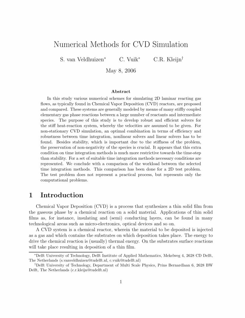
Besides the chemical model of the reacting gases, also some other properties of the gasmixture are needed. As mentioned before, the inlet temperature of the mixture is 300 K,and the temperature at the susceptor is 1000 K. The pressure in the reactor is 1 atm.,which is equal to 1.013 · 105 Pa. Other properties are given in Table 3. The diffusioncoefficients, according to Fick’s Law, are given in Table 4.

Density ρ(T ) 1.637 · 10−1 · 300T

[kg/m3]

Specific heat cp 5.163 · 103 [J/kg/K]

Viscosity µ 1.990 · 10−5(

T300

)0.7[kg/m/s]

Thermal conductivity λ 1.547 · 10−1(

T300

)0.8[W/m/K]

Table 3: Gas mixture properties

SiH4 4.77 · 10−6(

T300

)1.7

SiH2 5.38 · 10−6(

T300

)1.7

H2SiSiH2 3.94 · 10−6(

T300

)1.7

Si2H6 3.72 · 10−6(

T300

)1.7

Si3H8 3.05 · 10−6(

T300

)1.7

H2 8.02 · 10−6(

T300

)1.7

Table 4: Diffusion coefficients D′i, according to Fick’s Law

3 Solution Methods for the Species Equations

The species equations (8) are PDEs of the advection-diffusion-reaction type. In orderto have a unique solution appropriate boundary conditions and initial values have to bechosen. For a complete description we refer to [9, 16].

In general, it is impossible to find the exact solution of the system of N − 1 coupledspecies equation. Therefore, we have to approximate its solution by numerical methods.To do this, we use the Method of Lines, shorter MOL, where the PDE (or system of PDEs)is first discretized in space on a certain grid Ωh with mesh width h > 0 to yield a semidiscrete system

w′(t) = F (t, w(t)), 0 < t ≤ T, w(0) given, (13)

8

where w(t) = (wj(t))mj=1 ∈ Rm, with m proportional to the number of grid points in spatial

direction. The next step is to integrate the ODE system (13) with an appropriate timeintegration method.

We remark that the stiff reaction terms in CVD motivates to integrate parts of F (t, w(t))implicitly. In general, due to the nonlinearities in the reaction term, (huge) nonlinearsystems have to be solved. Most nonlinear solvers will need solutions of linear systems.

In order to approximate the solution of a system of species equations, choices have tobe made with respect to

1. Spatial Discretization,

2. Time Integration,

3. Nonlinear Solver, and

4. Linear Solver.

The topic of this research is to find the best combination in terms of efficiency. Of course,efficiency becomes a hot topic in the case of transient 3D simulations, where the simulationtimes become huge. In the case of 2D simulations the simulation times are, with thenowadays PCs,s, acceptable. Note that if the computational cost of one time step is (very)expensive, then a time integration method that needs more, but computational cheaper,time steps is better in terms of efficiency.

Besides the efficiency criteria, also some other properties are desired, for example posi-tivity, see Section 3.2. In order to make choices for spatial discretization, time integration,nonlinear and linear solvers, we formulate criteria in order of importance.

3.1 Stability

As already mentioned in Section 2 the system of species equations is stiff. First we paysome attention to this notion.

While the intuitive meaning of stiff is clear to all specialists, much controversy is goingon about it’s correct ‘mathematical definition’. We cite Hundsdorfer & Verwer [7] :

“Stiffness has no mathematical definition. Instead it is an operational concept,indicating the class of problems for which implicit methods perform (much)better than explicit methods.”

The eigenvalues of the Jacobian δfδy

play certainly a role in this decision, but quantities suchas the dimension of the system, the smoothness of the solution or the integration intervalare also important.

9

3.2 Positivity

An important property of chemical systems is positivity. By positivity we mean preser-vation of non-negativity for all components, which is a natural property for chemical speciesconcentrations. As a consequence, it should also hold for the mathematical model of theprocess. Whenever numerical simulations of reactive flows will be done, the positivityproperty has to be fulfilled on four levels, i.e.

1. Mathematical Model,

2. Spatial Discretization,

3. Time Integration, and,

4. Iterative Solvers (Newton-Raphson, Krylov Subspace Methods)

The first one is obvious. When a chemically reacting flow is modeled in a way that preser-vation of non-negativity of the solution is not guaranteed, then this property cannot holdfor the approximate solution.

Discretizing the PDE in space should not introduce ‘wiggles’, or (small) negative com-ponents, in the approximate solution, because then we (can) get blow up of the solutionin finite time.

When the semi-discretization preserves non-negativity, then also the time integrationmethod should preserve it. It appears that this extra condition on time integration meth-ods, besides stability, is much more restrictive towards the time step than stability. Wecome back to this in the next section.

Finally, when positivity is preserved on the previous levels, then this property alsohas to be fulfilled within the iterative solvers needed in the time integration. Recall that(non)linear systems will appear in this application because of stiff reaction terms. Espe-cially for the 3D simulations, and for 2D systems with a large number of species, iterativelinear solvers will be needed. This topic will become important for future research.

3.3 Efficiency

Having stiff reaction terms in the species equations implies doing parts of the timeintegration implicitly. As remarked before, choosing the ‘best’ time integration method interms of number of time steps, does not imply that this is the most efficient way to solvethe system of (N − 1) species equations.

Nonlinear Solvers

Integrating nonlinear ODEs implicitly gives rise to nonlinear equations F (x) = 0, x ∈Rn. In order to solve these equations one has a limited choice of methods. Roughlyspeaking, we have the following methods :

1. (Pseudo) Newton Iteration,

10

2. Fixed Point Iteration, and

3. Broyden’s Method.

To solve n dimensional systems F (x) = 0, with F : Rn → R

n and x ∈ Rn, the Newton

iteration is defined asxk+1 = xk − F ′(xk)−1F (xk). (14)

Importance of the above method rests on the fact that in a neighborhood of x the error‖xk+1 − x‖ (remark that x is a solution of F (x) = 0) can be estimated by the inequality

‖xk+1 − x‖ ≤ c‖xk − x‖2. (15)

Inequality (15) yields for a c ∈ R and a certain norm defined on Rn. The above inequalitystates that the (k + 1)th error is proportional to the kth error squared.

Difficulties with the Newton iteration are that in each step a linear system has to besolved. In practical applications where the dimensions of the linear systems can be up toone million, or even larger, an appropriate solver has to be found. It appears that thecomputational costs of one time step depends mainly on the linear solver as well as theevaluation of F (x) and F ′(x). Another difficulty is that convergence of the iteration isassured in a neighborhood of the solution. To get global convergence one can extend theNewton algorithm with, for example, line-search. Adding the line-search will guaranteethat the succeeding iterates are norm reducing in the sense that

‖F (xk+1)‖ ≤ ‖F (xk)‖ k = 0, 1, 2, . . . , (16)

for some norm defined on Rn. More on the topic of global convergence can be found in[8, 16].

The fixed point iteration has the advantage that it converges globally, as long as thespectral radius of the Jacobian of F (x) is less than one. A disadvantage is that we haveonly first order convergence. This method is only attractive when the function evaluationsare cheap.

Finally, the Broyden method is an extension of the secant method to n dimensions. Inorder to solve the scalar equation f(x) = 0 the secant method is given as

xk+1 = xk − f(xk)(xk − xk−1)

f(xk) − f(xk−1), (17)

where xk is the current iteration and xk−1 the iteration before. As can be found in [16],the secant method converges with order equal to the golden ratio. Broyden’s method isuseful in the case that the Jacobian is not explicitly available, or computable.

Linear Solvers

As mentioned above, the computational costs of one time step depends mainly on thecomputational costs of solving linear systems that appear in the nonlinear solver. Iterative

11

linear solvers will come into play for three dimensional systems. In the case that twodimensional systems are considered, one can suffice with direct solvers. Via reordering ofthe unknowns and the discrete species equations, one can obtain band matrices with a‘small’ bandwidth, such that the LU-factorization is still attractive.

4 Properties of Time Integration Methods

In this section we will pay more attention to the properties that are desired for thetime integration methods. The main focus will be on positivity. First, we start with some(mathematical) definitions on stability.

4.1 Stability Continued

Since we are dealing with stiff problems, stability is an important issue. It is preferredto use methods that are unconditionally stable, by which we mean that there is no step-sizerestriction with respect to stability. A formal definition is given below. Before giving thisdefinition we first have to define the so-called stability function.

Definition 4.1. Consider the scalar, complex Dahlquist test equation

y′ = λy, with λ ∈ C. (18)

Application of an one-step method, like for example Euler Forward or Runge-Kutta method,gives approximations

wn+1 = R(τλ)wn. (19)

The function R(z) (z = τλ) is called the stability function of the method. The set

S = z ∈ C : |R(z)| ≤ 1, (20)

is called the stability region of the method.

Definition 4.2. A method is called A-stable if the stability region S = z ∈ C : |R(z)| ≤ 1contains the left half plane C−.A method is called L-stable if the method is A-stable and |R(∞)| = 0.

In the case that |R(z)| are close to one for z with very large negative real part, the stiffparts of the approximate solution are damped out very slowly. To avoid difficulties withspecies with a short life span, which can appear in CVD, having L-stability is a desiredproperty for CVD simulation.

An other form of stability, to be defined in the definition below, is A(α)-stability. Thisform of stability comes from the stability analysis of multi-step methods. By a multi-stepmethod we mean that this method uses, unlike one-step methods like Euler Backward orRunge-Kutta methods, a fixed number of previous approximations. For more on multi-stepmethods we refer to [16, 5, 7].

12

Definition 4.3. A method is called A(α)-stable (for α < π2) if the stability region S =

z ∈ C : |R(z)| ≤ 1 is a subset of

S ⊃ z ∈ C− : z = 0,∞ or |arg(−z)| ≤ α (21)

From the above definition we see that A(α)-stability is a weaker form of stability thanA-stability. For certain values of α, also these methods are interesting for time integrationof species equations.

Example 4.1. The BDF methods, see Section 5.1, are for k = 1, 2 A-stable. For 3 ≤ k ≤ 6the BDF methods is A(α)-stable, with α depending on k. See Table 5.

k 1 2 3 4 5 6

α in rad π2

π2

1.501 1.2741 0.8901 0.2967

α in degrees 90 90 86 73 51 17

Table 5: Values of α, in both radials as degrees, for given k.

−4 −3 −2 −1 0 1 2−3

−2

−1

0

1

2

3Stability Region for BDF−2

−4 −3 −2 −1 0 1 2−3

−2

−1

0

1

2

3Stability Region for BDF−3

Figure 2: Stability regions of the BDF-2 method (left) and the BDF-3 method (right).

In Figure 2 the stability regions for the BDF-2 method and the BDF-3 method2 aregiven. Notice that the BDF-3 method is indeed not A-stable, as can be seen in Figure 2.

IMEX

Instead of using a fully implicit time integration, one can also integrate only the ex-tremely stiff part in an implicit way. Suppose we have the nonlinear system or semi-discretization

w′(t) = F (t, w(t)),

2BDF methods are extensively described in, for example, [7, 5, 16]

13

where F (t, w(t)) has the natural splitting

F (t, w(t)) = F0(t, w(t)) + F1(t, w(t)),

with F0 is a non-stiff and F1 stiff. In advection-diffusion-reaction systems the non-stiffterm is for instance advection and the stiff terms the discretized diffusion and reactions.The non-stiff term is suitable for explicit time integration while the stiff terms are moresuitable for implicit integration methods.

An example of a method that combines explicit as well as implicit treatment of respec-tively the non-stiff term F0(t, w(t)) and stiff term F1(t, w(t)) is the following one :

wn+1 = wn + τ (F0(tn, wn) + (1 − θ)F1(tn, wn) + θF1(tn+1, wn+1)) , (22)

where the parameter θ ≥ 12. This method is a combination of the Euler Forward method,

which is explicit, and the implicit θ -method. Methods that are mixtures of IMplicit andEXplicit methods are called IMEX methods. The method given in (22) is called the IMEX-θ Method.

Consider the test equation

w′(t) = λ0w(t) + λ1w(t),

and let zj = τλj for j = 0, 1. Applying the IMEX- θ method to this test equation gives

R(z0, z1) =1 + z0 + (1 − θ)z1

1 − θz1. (23)

Stability of the IMEX- θ method thus requires

|R(z0, z1)| ≤ 1. (24)

To analyze the stability region (24) we have two starting points :

1. Assume the implicit part of the method to be stable, in fact A-stable, and investigatethe stability region of the explicit part,

2. Assume the explicit part of the method to be stable and investigate the stability regionof the implicit part.

Starting with the first point, we assume the implicit part of the IMEX- θ method to beA-stable. Define the set

D0 = z0 ∈ C : the IMEX scheme is stable ∀z1 ∈ C−,

where C− is the setC

− = z ∈ C : Re z ≤ 0.The question is whether the set D0 is smaller, larger or equally shaped in comparison withthe stability region of Euler Forward. The boundary of the region D0 is given in Figure

14

3. For a detailed derivation of this boundary, we refer to [16]. A similar way of reasoningcan be done to derive the boundary of D1, whereby

D1 = z1 ∈ C : the IMEX scheme is stable ∀z0 ∈ S0, (25)

and S0 the stability region of Euler Forward. The boundary of D1 is also given in Figure3.

We remark that for θ = 1 the IMEX method has favorable stability properties. It couldbe seen as a form of time splitting where we first solve the explicit part with Euler Forwardand the implicit part with Euler Backward. However, using this IMEX method we do nothave errors as consequence of

• intermediate results that are inconsistent with the full equation,

• intermediate boundary conditions to solve these intermediate results.

If one uses this IMEX- θ method with θ = 12, then one has to pay a little more attention

to stability. If, for instance, one has a system with complex eigenvalues, then the IMEXmethod will not be unconditionally stable for θ = 1

2.

The general idea of IMEX methods has been explained. We conclude with the remarkthat IMEX extensions can also be applied to multi-step methods, Runge-Kutta methodsand so on. The IMEX - θ method is the simplest example of an IMEX-Runge-Kuttamethod.

−3 −2.5 −2 −1.5 −1 −0.5 0 0.5 1−1.5

−1

−0.5

0

0.5

1

1.5

−3 −2.5 −2 −1.5 −1 −0.5 0 0.5 1

−1.5

−1

−0.5

0

0.5

1

1.5

Figure 3: Boundary of regions D0 (left) and D1 (right) for θ = 0.5 (circles), 0.51 (-·-), 0.6 (- -) and 1 (solid)

4.2 Positivity

Definition 4.4. An ODE system

w′(t) = F (t, w(t)) t ≥ 0, (26)

is called positive, or non-negativity preserving, if

w(0) ≥ 0 =⇒ w(t) ≥ 0, for all t > 0. (27)

15

It is easy to prove, for instance by using Theorem 4.5, which is given below, that linearsystems

w′(t) = Aw(t), w(t) ∈ Rn, A ∈ R

n×n, A = (aij), (28)

are positive if and only if aij ≥ 0 for i 6= j. The next theorem provides a simple criterionon F (t, w(t)) to tell us whether the system

w′(t) = F (t, w(t)) t ≥ 0, (29)

is positive.

Theorem 4.5. Suppose that F (t, w) is continuous and satisfies a Lipschitz condition withrespect to w 3. Then the system (29) is positive if and only if for any vector w ∈ Rm andall i = 1, . . . , m and t ≥ 0,

w ≥ 0, wi = 0 =⇒ Fi(t, w) ≥ 0. (30)

Proof. For a proof we refer to [7, Theorem 7.1, p.116]

It is interesting to investigate the positivity for semi-discrete systems. Consider, forinstance, the linear advection-diffusion equation in one dimension, i.e.,

ut + (a(x, t)u)x = (d(x, t)ux)x, (31)

whereby a(x, t) is the space and time dependent advection coefficient, and d(x, t) the spaceand time dependent diffusion coefficient. Furthermore, d(x, t) > 0 and spatial periodicboundary conditions are assumed.

Discretizing (31) by means of central differences gives

w′j =

1

2h

(

aj− 12(wj−1 + wj) − aj+ 1

2(wj + wj+1)

)

+

1

h2

(

dj− 12(wj−1 − wj) − dj+ 1

2(wj − wj+1)

)

, (32)

for j = 1, . . . , m, where wj = wj(t), w0 = wm, wn+1 = w1 and

aj± 12

= a(xj± 12, t), dj± 1

2= a(xj± 1

2, t). (33)

Using Theorem 4.5 it follows, after an elementary calculation, that the central discretization(32) is positive if and only if the cell Peclet numbers, defined as ah/d, satisfy

maxx,t

|a(x, t)|hd(x, t)

≤ 2. (34)

3The condition‖F (t, v) − F (t, v)‖ ≤ L‖v − v‖,

with v, v ∈ Rm and F : R × Rm → Rm, is called a Lipschitz condition with Lipschitz constant L.

16

Discretizing (31) by means of first order upwind for the advection part, and second ordercentral differences for the diffusive part, gives

w′j =

1

h

(

a+j− 1

2

wj−1 + (a+j− 1

2

− a−j− 1

2

)wj + a−j− 1

2

wj+1))

1

h2

(

dj− 12(wj−1 − wj) − dj− 1

2(wj − wj+1)

)

, (35)

where a+ = max(a, 0) and a− = min(a, 0). Hence, the semi-discrete system (35) is uncon-ditionally positive.

Positivity of Semi-Discrete Species Equations

Adding reaction terms to (31) does not influence the positivity. Since the reactionterms that are being add are in the production-loss form

F (t, v) = p(t, v) − L(t, v)v, (36)

where p(t, v) is a vector and L(t, v) a diagonal matrix. It can be found in [7] that sourceterms in this form are positive as long as p(t, v) is positive.

Furthermore, we mention that the above results with respect to the one-dimensionaladvection-diffusion equation are easily generalized to higher dimensions. Therefore, dis-cretizing the species concentrations equations in space by means of a hybrid scheme4 ensurespositivity of the semi-discretization.

A last remark with respect to upwind discretization. For higher order upwinding, forexample third order upwinding, positivity is not ensured for all step-sizes.

Positivity on the Level of Time Integration

Positivity also restricts the use of time integration methods. It appears that uncondi-tional positivity is a very restrictive requirement. In this section we will present resultsfor non-linear systems w′(t) = F (t, w(t)). First we begin with exploring the positivityproperty for Euler Forward and Backward.

Euler Forward and Backward

We consider the non-linear semi-discretization w′(t) = F (t, w(t)). Suppose that F (t, w(t))satisfies the condition :

Condition 4.6. There is an α > 0, with α as large as possible, such that ατ ≤ 1 and

v + τF (t, v) ≥ 0 for all t ≥ 0, v ≥ 0. (37)

4The hybrid scheme uses central differences, except in the regions where |Pe| > 2. In the regions with|Pe| > 2 first order upwind is used.

17

Application of Euler Forward to the nonlinear system w′(t) = F (t, w(t)) gives

wn+1 = wn + τF (tn, wn). (38)

Provided that wn ≥ 0, Condition 4.6 guarantees positivity for wn+1 computed via EulerForward (38).

Furthermore, assume that F (t, w(t)) also satisfies the following condition :

Condition 4.7. For any v ≥ 0, t ≥ 0 and τ > 0 the equation

u = v + τF (t, u), (39)

has a unique solution that depends continuously on τ and v.

According to the following theorem we have unconditional positivity for Euler Back-ward.

Theorem 4.8. Conditions 4.6 and 4.7 imply positivity for Euler Backward for any stepsize τ .

The following proof is taken from [7].

Proof of Theorem 4.8. For given t, v and with τ variable we consider the equation u =v + τF (t, u) and we call its solution u(τ). We have to show that v ≥ 0 implies u(τ) ≥ 0 forall positive τ . By continuity it is sufficient to show that v > 0 implies u(τ) ≥ 0. This istrue because if we assume that u(τ) > 0 for τ ≤ τ0, except for the ith component ui(τ0) = 0,then

0 = ui = vi + τ0Fi(t, u(τ0)). (40)

According to Condition 4.6 we have Fi(t, u(τ0)) ≥ 0 and thus vi + τ0Fi(t, u(τ0)) > 0, whichis a contradiction.

Remark 4.9. Unlike Condition 4.6, Condition 4.7 is not easy to be verified. As remarkedin [7], it is sufficient to hold that F (t, v) is continuously differentiable and

‖I − τJF (t, v)‖ ≤ C, for any v ∈ Rn, t ≥ 0 and τ > 0, (41)

whereby C is a positive constant and JF (t, v) the Jacobian of F (t, v) with respect to v.Existence and uniqueness of the solution of

u = v + τF (t, u), (42)

then follows from Hadamard’s Theorem and the Implicit Function Theorem. The fact thatthe solution u of (42) depends continuously of τ , v and t also follows from the ImplicitFunction Theorem. Remark that condition (41) is easier to verify than Condition 4.7.Both Hadamard’s Theorem and the Implicit Function Theorem can be found, for example,in [11].

18

Remark 4.10. Application of Euler Backward to the nonlinear system w′(t) = F (t, w(t))gives

wn+1 − τF (tn, wn+1) = wn. (43)

As proven in Theorem 4.8, for every time step τ positivity of wn+1 is ensured as long aswn is positive and F (t, w) satisfies conditions (4.6) and (4.7). In practice it is impossibleto compute the solution wn+1 of the nonlinear equation (43) exactly, thus one will use aniterative nonlinear solver. For example, the Newton Raphson iteration is in most applica-tions a good choice. Since iterative nonlinear solvers will only give an approximation ofthe solution, it might be possible that it contains (small) negative components. Therefore,in practice even Euler Backward can produce negative concentrations.

As mentioned before, negative components of the concentration solution vector cancause a blow up in finite time. In the case the negative components of the solution arethe result of rounding errors, then it is justified to set them to zero. We remark that inthe case of rounding errors the negative components are very small (compared with therelative error, condition number and the machine precision). In the case one has negativecomponents in the solution as consequence of the nonlinear (Newton) solver, then the mostcommon method to avoid negative concentrations is clipping. A disadvantage of applyingclipping is that mass is added, i.e., the integration method does not preserve mass anylonger. A possible solution is given in [12], where for the positive integration of chemicalkinetic systems a projection method is proposed. This projection method works as follows.First, a numerical approximation is computed via a traditional (read Runge Kutta orRosenbrock method) scheme, which preserves mass. If there are negative components inthe solution, then the nearest vector in the reaction simplex is found using a primal-dualoptimization routine. The resulting vector, is a better approximation of the true solutionand preserves mass. In the case of advection-diffusion-reaction systems, no references areavailable to do this.

Some General Remarks on Positivity

In the previous section it has been proven that the Euler Backward method is un-conditionally positive, when Conditions 4.6 and 4.7 are satisfied. We remark that theseconditions are actually conditions on F (t, v). Unconditional positivity can only be true forimplicit methods. One might hope to find more accurate methods with this unconditionalpositivity property. However, this hope is dashed by the following result, which holds forboth linear and nonlinear systems, due to Bolley and Crouzeix [2].

Theorem 4.11. Any method that is unconditionally positive, has order p ≤ 1.

For a proof we refer to [2]. The consequence of this theorem is that the only well-knownmethod having unconditionally positivity is Euler Backward.

Finally, we remark that for higher order methods the time step can be restricted toimpractically small values. Furthermore, we mention that for Diagonally Implicit RungeKutta (DIRK) methods step size restrictions are known, such that positivity is guaranteed.We refer to [7, 16].

19

4.3 Relation Positivity and TVD

If the system of ODEs w′(t) = F (t, w(t)), with a appropriate initial condition w(0) =w0, stands for a semi-discrete version of a conservation law, it is important that the fullydiscrete process is monotonic in the sense that

‖wn‖ ≤ ‖wn−1‖. (44)

The above monotonicity property reduces to the Total Variation Diminishing (TVD) prop-erty when we use the seminorm

|y|TV =n∑

j=1

|yj − yj−1|, with y0 = yn, for y ∈ Rn, (45)

in (44). When a numerical scheme satisfies this TVD property, then localized over- andundershoots are prevented.

The TVD property is developed for studying the properties of numerical schemes forsolving hyperbolic conservation laws. In particular TVD and monoticity are important inthe study of shocks in fluid flows.

In this section we will discuss some general results for TVD. It turns out that theconditions giving the TVD property are the same as giving the positivity property.

TVD Results for ODE Methods

Considering the ODE system w′(t) = F (t, w(t)) with a function F such that

|v + τF (t, v)| ≥ |v| for all t ≥ 0, for allv ∈ Rn and 0 ≤ τ ≤ τ ∗. (46)

Then, the above condition can be seen as a condition on the time step τ such that EulerForward is TVD.

We remark that this condition is equivalent with the condition for positivity for EulerForward (4.6). This can be seen as follows. Considering a positive nonlinear systemw′(t) = F (t, w(t)), we have to find an α such that (4.6) holds. Taking

α =1

τ ∗, (47)

and considering v ≥ 0, then (46) implies v + τF (t, v) ≥ 0.Applying the Backward Euler method to w′(t) = F (t, w(t)) gives

wn+1 = wn + τF (tn+1, wn+1). (48)

This method is TVD under Assumption (46) without any step size restriction. This caneasily be seen from

(

1 +τ

τ ∗

)

wn+1 = wn +τ

τ ∗(wn+1 + τ ∗F (tn+1, wn+1).) (49)

20

Using the TV seminorm we obtain

(

1 +τ

τ ∗

)

|wn+1|TV ≤ |wn|TV +τ

τ ∗|wn+1|TV , (50)

showing that |wn+1|TV ≤ |wn|TV for any τ > 0.For other one-step methods like Diagonally Implicit Runge Kutta methods step size

restrictions can be derived to have the TVD property. These conditions are identical tothose for positivity of DIRK methods. For TVD results for multistep, or other generalresults for TVD we refer to [3, 7, 20]. In [3] the rather disappointing result concerningthe nonexistence of implicit TVD Runge Kutta or multistep methods of order higher than1 has been proven. By adding some explicit stages to an explicit higher order RK ormultistep scheme the TVD property can be recovered. In our case of stiff systems, thislast artifact to save the TVD property is useless, because then the stiff reaction parts haveto be integrated explicitly.

To conclude this section we would like to remark the following. With respect to positiv-ity and TVD, implicitness of the method seems to have little added value, in clear contrastwith stability. For example, the implicit trapezoidal rule

wn+1 = wn +τ

2(F (tn, wn) + F (tn+1, wn+1)) , (51)

has a time step restriction in order to be TVD, when applied to time integration of ut +a ·ux = 0, whereby the advection term is discretized using limiters. Then, as can be foundin [7, 20], the TVD property holds if the Courant number ν = τa/h ≤ 1. Comparing thiswith the Euler Backward method, which is unconditionally TVD, we see that implicitnesshas little added value in this case.

4.4 Concluding Remarks on Stability, Positivity and TVD

In order to integrate the species equations we need a method that can handle stiffproblems and that is unconditionally positive or has the TVD property. In this section thefollowing notions passed the revue:

• Explicit,

• Implicit,

• Stiff,

• Positivity,

• At Most First order Accurate,

• Higher Order Integration Methods,

• TVD,

21

• IMEX.

A time integration method that would be suitable to integrate the species equations needsto have a few of the above mentioned properties. Combinations of the properties that arepossible are :

1. Positivity, Implicit, At Most First order Accurate and Stiff,

2. TVD, Implicit, At Most First order Accurate and Stiff,

3. IMEX, Higher Order Integration Methods, Positivity or TVD, Stiff,

4. Explicit, Higher Order Integration Methods, TVD,

5. Implicit, TVD, Higher Order Integration Methods, Adding explicit stages.

The last two combinations of properties, i.e., 4. and 5., are not suitable for solving the stiffspecies equations, because they contain explicit stages. Integrating the reactions termsexplicitly will give a strong restriction on the time step. The latter is not preferred inpractice.

5 Suitable Methods to Integrate

In this section we present integration methods that are suitable, from a theoreticalpoint of view, for the time integration of the species equations. At the end of this sectionwe will also mention nonlinear - and linear solvers.

From the previous sections it became clear that the Euler Backward method is a suit-able method to perform time integration. It has the advantages of being unconditionallystable and positive. Disadvantages are the first order consistency and the probably highcomputational costs for one time step. The latter is due to the fact that the succeedingapproximations are computed in a fully implicit manner.

5.1 Time Integration Methods

We will discuss a selection of time integration methods that have good properties inboth stability and positivity, or TVD.

Rosenbrock Methods

Definition 5.1. An s-stage Rosenbrock method is defined as

ki = τF (wn +i−1∑

j=1

αijkj) + τAi∑

j=1

γijkj ,

wn+1 = wn +

s∑

i=1

biki (52)

22

where A = An is the Jacobian F ′(w(t)).

Definition 5.1 is taken from [7]. The coefficients bij , αij and γij define a particularmethod and are selected to obtain a desired level of consistency and stability.

Remark that computing an approximation wn+1 from wn, in each stage i a linear systemof algebraic equations with the matrix (I − γiiτA) has to be solved. To save computingtime for large dimension systems w′(t) = F (w(t)) the coefficients γii are taken constant,e.g., γii = γ. Then, in every time-step the matrix (I − γiiA) is the same. To solve theselarge systems LU decomposition or (preconditioned) iterative methods could be used.

Define

βij = αij + γij, ci =i−1∑

j=1

αij and di =i−1∑

j=1

βij.

In Table 5.1, taken from [7], the order conditions for s ≤ 4 and p ≤ 3 and γii = γ =constant can be found. In particular the two stage method

order p order conditions

1 b1 + b2 + b3 + b4 = 1

2 b1d2 + b3d3 + b4d4 = 12− γ

3 b2c22 + b3c

23 + b4d

24 = 1

3

b3β32d2 + b4(β42d2 + β43d3) = 16− γ + γ2

Table 6: Order conditions of Rosenbrock methods with γii = γ for s ≤ 4 and p ≤ 3.

wn+1 = wn + b1k1 + b2k2

k1 = τF (wn) + γτAk1

k2 = τF (wn + α21k1) + γ21τAk1 + γτAk2, (53)

with coefficients

b1 = 1 − b2, α21 =1

2b2and γ21 = − γ

b2,

is interesting. This method is of order two for arbitrary γ as long as b2 6= 0 . The stabilityfunction is given as

R(z) =1 + (1 − 2γ)z + (γ2 − 2γ + 1

2)z2

(1 − γz)2. (54)

The method is A-stable for γ ≥ 14

and L-stable if γ = 1 ± 12

√2. By selecting for γ the

larger value γ+ = 1 + 12

√2, we have the property that R(z) ≥ 0, for all negative real z.

For diffusion-reaction problems, which have negative real eigenvalues, this property ensurespositivity of the solution. In the case that advection is added to the system, the matrixhas eigenvalues with negative real parts and relatively small imaginary parts. Then, the

23

positivity property is no longer guaranteed. It appears that the second order Rosenbrockmethod performs quite well with respect to the positivity property, as has been experiencedin [17]. In [17] it is conjectured that the property that R(z) ≥ 0 for all negative realz plays a role. We conclude this section with a remark on the implementation of thesecond order Rosenbrock scheme (56). In our code it is implemented with the parametersb1 = b2 = 1

2and γ = 1+ 1

2

√2. The matrix-vector multiplication in the second stage of (56)

can be avoided by introducing

k1 = k1 and k2 = k2 − k1, (55)

and implementing the scheme

wn+1 = wn +3

2k1 +

1

2k2,

k1 = τF (wn) + γτAk1,

k2 = τF (wn + k1) − 2k1 + γτAk2. (56)

Backward Differentiation Formulas (BDF)

The Backward Differentiation Formulas, shorter BDF, belong to the class of linearmultistep methods, as defined in Definition 5.2

Definition 5.2. The linear k-step method is defined by the formula

k∑

j=0

αjwn+j = τ

k∑

j=0

βjF (tn+j, wn+j), n = 0, 1, . . . , (57)

which uses the k past values wn, . . . , wn+k−1 to compute wn+k. Remark that the mostadvanced level is tn+k instead of tn+1.

The method is explicit when βk = 0 and implicit otherwise. Furthermore, we willassume that αk > 0.

The BDF are implicit and defined as

βk 6= 0 and βj = 0 for j = 0, . . . , k − 1.

The coefficients αi, see Definition 5.2, are chosen such that the order is optimal, namelyk. 5 The 1-step BDF method is Backward Euler. The 2-step method is

3

2wn+2 − 2wn+1 +

1

2wn = τF (tn+2, wn+2), (58)

5A linear k-step method is of order p if and only if

k∑

i=0

αi = 0k∑

i=0

αiij = 0 = j

k∑

i=0

βiij−1 for j = 1, 2, . . . , p.

For a proof we refer to [16].

24

and the three step BDF is given by

11

6wn+3 − 3wn+2 +

3

2wn+1 −

1

3wn = τF (tn+3, wn+3). (59)

In chemistry applications the BDF methods belong to the most widely used methods tosolve stiff chemical reaction equations, due to their favorable stability properties. TheBDF-1 and BDF-2 methods are both A-stable. The 3,4,5 and 6 step BDF methods areA(α)-stable, with α given in Example 4.1. For k > 6 the BDF-methods are unstable, see[4, Theorem 3.4, page 329].

Remark 5.3. A disadvantage of linear multi-step methods is that the first k − 1 approx-imations cannot be computed with the linear k-step scheme. To compute the first (k − 1)approximations, one could use a

1. Runge-Kutta scheme, for example, Euler Backward, or,

2. use for the first step a linear 1-step method, for the second approximation a linear2-step method, . . . and for the (k − 1)st approximation a linear (k − 1)-step scheme.

As for Runge-Kutta methods the requirement of positivity does place a severe step sizerestriction on (implicit) BDF methods (and also on implicit multistep methods). UnderCondition 4.6 and 4.7 we obtain positivity of w′(t) = F (t, w(t)) whenever ατ ≤ γR. Theparameter γR is the largest γ such that the stability function R(z) is absolutely monotonicon [−γ, 0]. It is easy to check that for the BDF-2 method we have γR = 1

2. Thus, positivity

for BDF-2 is ensured whenever

ατ ≤ 1

2, (60)

provided that w1 is computed from w0 by a suitable starting procedure. By suitable wemean that w1 has to be computed from a method that ensures w1 to be positive, suchas for example BDF-1 (which is Euler Backward). Implementation of the methods isstraightforward.

IMEX Runge-Kutta Chebyshev Methods

The IMEX extension of the class of Runge-Kutta Chebyshev methods is developed byVerwer et. al. [18, 19]. The Runge-Kutta Chebyshev methods belong to the class ofexplicit Runge-Kutta Chebyshev methods. They posses an extended real stability intervalwith a length proportional to s2, with s the number of stages.

Definition 5.4. The stability boundary β(s) is the number β(s) such that [−β(s), 0] is thelargest segment of the negative real axis contained in the stability region

S = z ∈ C : |R(z)| ≤ 1 .

25

To construct the family of RKC methods we start with the explicit Runge-Kutta meth-ods which have the stability polynomial

R(z) = γ0 + γ1z + · · ·+ γszs. (61)

In order to have first order consistency we take γ0 = γ1 = 1.6

It can be proven that every explicit Runge-Kutta method has as optimal stabilityboundary β(s) = 2s2. Thus the maximum value of β(s) for explicit Runge-Kutta methodsis 2s2. The upper boundary of β(s) is achieved if we take the shifted Chebyshev polynomialsof the first kind as stability polynomial. For a proof of both results, we refer to [7, 16].

In this paper we will not go into further details on the construction of the second orderscheme. We fulfill with presenting it. The second order RKC is given as

wn0 = wn,

wn1 = wn + µ1τF (tn + c0τ, wn0),

wnj = (1 − µj − νj)wn + µjwn,j−1 + νjwn,j−2 + j = 1, . . . , s

+µ1τF (tn + cj−1τ, wn,j−1) + γjτF (tn + c0τ, wn0), (63)

wn+1 = wns,

with coefficients

ω0 = 1 +ε

s2, ω1 =

T ′s(ω0)

T ′′s (ω0)

, (64)

bj =T ′′

j (ω0)

(T ′j(ω0))2

, cj =T ′

s(ω0)

T ′′s (ω0)

T ′′j (ω0)

T ′j(ω0)

≈ j2 − 1

s2 − 1, (65)

µ1 = b1ω1, µj =2bjω0

bj−1, νj = − bj

bj−2, (66)

µj =2bjω1

bj−1, γj = −aj−1µj . (67)

The stability function of this method is given as

Bs(z) = 1 +T ′′

s (ω0)

(T ′s(ω0))2

(Ts(ω0 + ω1z) − Ts(ω0)) (68)

with

ω0 = 1 +ε

s2ω1 =

T ′s(ω0)

T ′′s (ω0)

.

6This can be verified by considering the test equation y′ = λy. The local error of the test equationsatisfies

ez − R(z)

τ= O(τp). (62)

To achieve pth order consistency the coefficients γi has to be chosen in such a way that (62) satisfies for p.

26

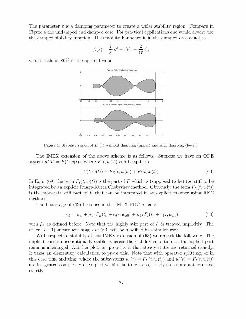
The parameter ε is a damping parameter to create a wider stability region. Compare inFigure 4 the undamped and damped case. For practical applications one would always usethe damped stability function. The stability boundary is in the damped case equal to

β(s) =2

3(s2 − 1)(1 − 2

15ε),

which is about 80% of the optimal value.

−20 −18 −16 −14 −12 −10 −8 −6 −4 −2 0 2−5

0

5Second Order Chebyshev Polynomial

−20 −18 −16 −14 −12 −10 −8 −6 −4 −2 0 2−5

0

5Second Order Damped Chebyshev Polynomial

Figure 4: Stability region of B5(z) without damping (upper) and with damping (lower).

The IMEX extension of the above scheme is as follows. Suppose we have an ODEsystem w′(t) = F (t, w(t)), where F (t, w(t)) can be split as

F (t, w(t)) = FE(t, w(t)) + FI(t, w(t)). (69)

In Eqn. (69) the term FI(t, w(t)) is the part of F which is (supposed to be) too stiff to beintegrated by an explicit Runge-Kutta Chebyshev method. Obviously, the term FE(t, w(t))is the moderate stiff part of F that can be integrated in an explicit manner using RKCmethods.

The first stage of (63) becomes in the IMEX-RKC scheme

wn1 = wn + µ1τFE(tn + c0τ, wn0) + µ1τFI(tn + c1τ, wn1), (70)

with µ1 as defined before. Note that the highly stiff part of F is treated implicitly. Theother (s − 1) subsequent stages of (63) will be modified in a similar way.

With respect to stability of this IMEX extension of (63) we remark the following. Theimplicit part is unconditionally stable, whereas the stability condition for the explicit partremains unchanged. Another pleasant property is that steady states are returned exactly.It takes an elementary calculation to prove this. Note that with operator splitting, or inthis case time splitting, where the subsystems w′(t) = FE(t, w(t)) and w′(t) = FI(t, w(t))are integrated completely decoupled within the time-steps, steady states are not returnedexactly.

27

We conclude with some remarks on the implementation and use of the IMEX-RKCschemes in practice. We use a variable time step controller as is normal for Method ofLines solvers. Then, it would be desirable that for relatively small τn the code automaticallyswitches to a lower number of stages s. For relatively large τn the same is desired, of course.This is only important for the integration of advection diffusion part of the right hand sideof (13).

We will briefly describe the idea behind this variable number of stages procedure,which is taken from [19]. In [20] time step size conditions are given for the standard spatialdiscretizations of the m-dimensional scalar model

ut +m∑

k=1

akuxk= d

m∑

k=1

uxkxk, (71)

guaranteeing eigenvalues emerging from von Neumann stability analysis to lie inside geo-metric figures like squares, ellipses, half ellipses and ovals. For the explicit integration ofadvection and diffusion via the RKC method one has to fit an appropriate figure inside thestability region S. In [19] ovals are selected. In Figure 12 stability regions with inscribedovals

(

x

β/2+ 1

)2

+( y

α

)4

= 1, (72)

for s = 6 and ε = 0.1, 1, 10. Recall that epsilon is a damping factor, see (64). For β thevalue β(s) has been taken, while α has been derived numerically. Assume that for diffusion

−25 −20 −15 −10 −5 0

−5

0

5

s = 6, ε = 0.1, α = 0.798, β = 23.056

(a)

−20 −15 −10 −5 0

−5

0

5

s = 6, ε = 1, α = 2.255, β = 20.944

(b)

−14 −12 −10 −8 −6 −4 −2 0 2

−5

0

5

s = 6, ε = 10, α = 3.63, β = 14.116

(c)

Figure 5: Stability regions S and inscribed ovals.

28

second order central discretization, while for advection the κ-scheme

dw

dt=

a

4h((1 − κ)wj−2 + (3κ − 5)wj−1 + (3 − 3κ)wj + (1 + κ)wj+1), (73)

is used. The κ-scheme is the second order central scheme for κ = 1, the second orderupwind scheme for κ = −1 and third order upwind-biased scheme for κ = 1

3. The diffusion

step size condition is then the familiar condition

τ ≤ β(s)

2d∑m

k=1 h−2k (2 + (1 − κ)Pk)

, (74)

where Pk = |ak |hk

dis a mesh Peclet number. Violation of (74) will give instability. Also

taken from [20] is the advection time step restriction

τ ≤ q1

(

4dα4(s)

β(s)

)13

/

m∑

k=1

(

a4k

h2k

)13

, (75)

where the parameter q1 depends on the choice of κ, see Table 5.1. For the actual imple-

κ q113

0.6351 1−1 0.323

Table 7: Values for q1 for popular κ values

mentation the following lower bound for the ratio α4(s)β(s)

has been used

α4(s)

β(s)=

2 s = 2,4(6 − s) + 6.15(s − 4) s = 4, 6,

6.15 (10−s)2

+ 15.5 (s−6)4

s = 8,15.5 s = 10, 12, . . .

(76)

As maximum of the ratio α4(s)β(s)

the value 15.5 has been taken, which corresponds withs = 10. For larger values of s the slope in the curve, by which we mean the upper half ofthe oval (72), becomes too small.

Next, we will describe how to choose the number of stages s. Suppose a step size τ ∗

has been obtained by a local error estimator. Then, it can be checked whether τ ∗ satisfiesthe inequalities (74) and (75). If necessary, τ ∗ can be adjusted such that these inequalitieshold. Simultaneously, the number of stages can be adjusted such that the number of stagesneeded to satisfy (74) is larger or equal than the number of stages needed to satisfy (75).

29

We remark that it makes no sense to spend more stages on advection than required fordiffusion. Introduce the parameters

Ψ1 =1

2d∑m

k=1 h−2k (2 + (1 − κ)Pk)

, and, Ψ2 =4dq3

1(

∑mk=1

(

a4k

h2k

)13

)3 . (77)

The actual algorithm that is used in the code is given in Algorithm 1. For more background

Algorithm 1 Step size and Number of Stages Selection

1: If τ ∗ ≤ 2Ψ1, then s = 2, τ = minτ ∗, (2Ψ)1/3 and stop,2: Put τ = minτ ∗, (15.5Ψ)1/3. If τ ∗ ≤ 2Ψ1, then s = 2 and stop,3: Determine sd ≥ 4 such that τ ≤ β(sd)Ψ1 to satisfy (74),4: Determine sa ≥ 4 such that τ ≤ ((α4(sa)/β(sa))Ψ2)

1/3 to satisfy (75),5: If sa ≤ sd, then s = sd and stop. Otherwise τ = 0.8τ and go to 3.

information we refer to [16, 18, 19].

5.2 Nonlinear Solvers

It is obvious that with the second order convergence the Newton iteration is a suitablechoice as nonlinear solver. The disadvantage of having local convergence will disappear ifone uses a line-search algorithm within the Newton solver. In order to have a decreasingsequence ‖F (xn)‖, we will adjust the Newton step d = −F ′(xn)−1F (xn)as follows. Findthe smallest integer m such that

‖F (xn + 2−md)‖ ≤ (1 − 2−m)‖F (xn)‖, (78)

and let the Newton-step be s = 2−md. Condition (78) is called the sufficient decrease of‖F‖. The parameter in (78) is a small number, chosen such that the sufficient decreasecondition is satisfied as easy as possible. In [8, 16] is taken equal to 10−4.

5.3 Linear Solvers

Because the nonlinear solver is of the Newton type, in each Newton iteration linearsystems have to be solved. In CVD literature one uses iterative linear solvers for both2D and 3D problems. We share the idea that for 3D problems iterative linear solvers aredefinitely needed. For 2D problems we think that direct solvers are still applicable.

2D Problems

In most 2D applications direct solvers like LU factorization are still applicable to solvelinear systems. To reduce the amount of work one usually reorders the unknowns (and the

30

equations), in order to reduce the bandwidth of the matrix. Also in our case it is possibleto reduce the bandwidth of the Jacobian considerably.

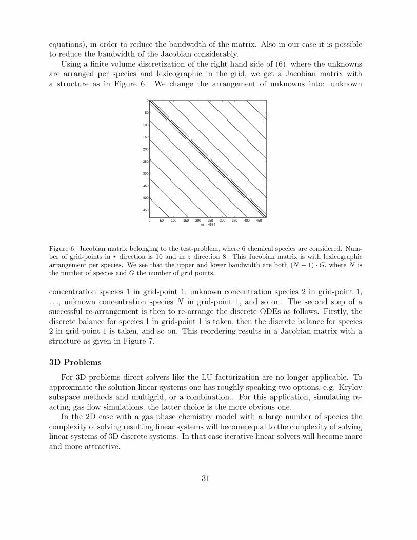
Using a finite volume discretization of the right hand side of (6), where the unknownsare arranged per species and lexicographic in the grid, we get a Jacobian matrix witha structure as in Figure 6. We change the arrangement of unknowns into: unknown

0 50 100 150 200 250 300 350 400 450

0

50

100

150

200

250

300

350

400

450

nz = 4584

Figure 6: Jacobian matrix belonging to the test-problem, where 6 chemical species are considered. Num-ber of grid-points in r direction is 10 and in z direction 8. This Jacobian matrix is with lexicographicarrangement per species. We see that the upper and lower bandwidth are both (N − 1) · G, where N isthe number of species and G the number of grid points.

concentration species 1 in grid-point 1, unknown concentration species 2 in grid-point 1,. . ., unknown concentration species N in grid-point 1, and so on. The second step of asuccessful re-arrangement is then to re-arrange the discrete ODEs as follows. Firstly, thediscrete balance for species 1 in grid-point 1 is taken, then the discrete balance for species2 in grid-point 1 is taken, and so on. This reordering results in a Jacobian matrix with astructure as given in Figure 7.

3D Problems

For 3D problems direct solvers like the LU factorization are no longer applicable. Toapproximate the solution linear systems one has roughly speaking two options, e.g. Krylovsubspace methods and multigrid, or a combination.. For this application, simulating re-acting gas flow simulations, the latter choice is the more obvious one.

In the 2D case with a gas phase chemistry model with a large number of species thecomplexity of solving resulting linear systems will become equal to the complexity of solvinglinear systems of 3D discrete systems. In that case iterative linear solvers will become moreand more attractive.

31

0 50 100 150 200 250 300 350 400 450

0

50

100

150

200

250

300

350

400

450

nz = 4584

Figure 7: Jacobian matrix belonging to the test-problem, where 6 chemical species are considered. Wehave the same number of grid-points in r and z direction. This Jacobian matrix is constructed with there-arrangement of the unknowns as described in Section 5.3. In this re-arranged case the bandwidth isequal to N · Gr, where Gr is the number of grid points in the r direction.

6 Numerical Simulation

Before giving the results of the numerical simulations, where we mainly considered theefficiency of the time integration methods, we give details on the simulation itself. Inthis simulation a variable time step algorithm is used, which will also be explained in thissection.

6.1 General Outline of the Simulation

We perform a transient simulation on the problem described in Section 2. The simula-tion stops when ‘numerical’ steady state is reached. By ‘numerical’ steady state we meanthat for a certain index n yields,

‖yn+1 − yn‖2

‖yn‖2

≤ ϑ, (79)

where yn is the numerical solution of the semi-discretization

dw

dt= Aw + b + F (t, w(t)), (80)

on time t = tn, and ϑ a small parameter. In (80) A represents the discretized advectiondiffusion operator, b a vector of boundary conditions and F (t, w(t)) a nonlinear vectorfunction representing the gas phase reactions. In our simulations for ϑ the value ϑ =O(10−6) has been taken.

32

In order to describe the algorithm that is used for CVD simulation we introduce thefunction ‘time integration’ as follows. As input we have yn, the approximated solution ofw on time t = tn, τ = tn+1− tn, m the molar mass field and f the vector of molar fractions.The output is yn+1, i.e., the approximated solution of w on time tn+1. Summarized

yn+1 = time integration(yn, τ, m, fi). (81)

The exact description of the function ‘time integration’ depends on the choice of timeintegration method. See Section 5.

Based on the inlet concentrations of silane SiH4 an initial mass fraction profile canbe constructed. The outline of the algorithm to perform the CVD simulation is given asAlgorithm 2. As mentioned earlier, for ϑ the value ϑ = 10−6 has been taken.

Algorithm 2 Simulation

1: Initial values for y0 and fi

2: while ‖y1−y0‖‖y0‖

≥ ϑ do3: Compute average molar mass of gas mixture m4: y1 = time integration(y0, τ, m, f)5: Check whether y1 ≥ 0, if not then τ = 1

2τ and go to 4

6: Estimate the local (time integration) error Dn

7: if Dn > Tol then8: τ = r · τ , r estimated such that Dn ≤ Tol, and go to 49: end if

10: Compute mole fractions f11: y0 = y1

12: end while

6.2 Variable Time Stepping

We briefly explain the variable time stepping algorithm as it is implemented in ourcode. Consider an attempted step from tn to tn+1 = tn + τn with time step size τn that isperformed with an pth order time integration method. Suppose an estimate Dn of orderp of the norm of the local truncation error is available. Then, if Dn < Tol this step τn isaccepted, whereas if Dn > Tol the step is rejected and redone with time step size 1

2τn. If

Dn < Tol, then the new step size is computed as

τnew = r · τ, r =

(

Tol

Dn

)1

p+1

. (82)

It is also possible to put bounds on the growth factor r of the new step size. This is simplydone by giving bounds on r.

33

6.2.1 Local Error Estimation for Euler Backward

The local error of the Euler Backward method

wn+1 = wn + τF (tn+1,wn+1) (83)

satisfies

δn = −1

2τ 2w′′(tn) + O(τ 3). (84)

The local truncation error δn can be estimated as

dn = −1

2(wn+1 − wn − τF (tn, wn)) . (85)

See, for example, [7].

6.2.2 Local Error Estimation for BDF2

For the BDF-2 scheme the local error estimation is as follows. Introduce the ratior = τn

τn−1, where τn is defined as above, e.g., τn = tn+1 − tn. The second order BDF-2

scheme can be rewritten in the form with the ratio r as

wn+2 −(1 + r2)

1 + 2rwn+1 +

r2

1 + 2rwn =

1 + r

1 + 2rτF (tn+2, wn+2). (86)

In a similar way as in Section 6.2.1 we obtain the first order estimator

dn =r

1 + r(wn+1 − (1 + r)wn + rwn−1) . (87)

A second order estimator, see [7], is

dn =1 + r

1 + 2r

(

wn+1 + (r2 − 1)wn − r2wn−1 − (1 + r)τnF (tn, wn))

. (88)

We remark that in the first time step, where BDF-1 is used, the local error is estimated by

d0 =1

2(w1 − w0 − τ0F (t0, w0)) . (89)

6.2.3 Local Error Estimation for IMEX-Runge-Kutta-Chebyshev

The local error estimation for the IMEX -Runge-Kutta-Chebyshev methods is the sameas for the explicit Runge-Kutta-Chebyshev schemes, see [19]. The asymptotically correctestimate of the local error is

dn =1

15[12(wn − wn+1) + 6τn(F (tn, wn) + F (tn+1, wn+1))] , (90)

which is taken from [14].

34

6.3 Numerical Results for the Simplified CVD System

In this part we present the numerical results of the simplified test problem as definedin Section 2.1 to 2.3. In this section we distinguish two different simulations, namely, thesimulation with physical initial conditions, see Section 6.3.1, and the simulation with aconstant initial profile, see Section 6.3.2.

The experiments are done in FORTRAN. The computations are done on a serial Pen-tium 4 (2.8 GHz) computer with 1Gb memory capacity. Moreover, the code is compiledwith FORTRAN g77 on LINUX.

6.3.1 Physical Initial Conditions

At t = 0 we start with the zero concentration profile for all species, except the carriergas, and let the reactive specie silane SiH4 enter the reactor at the inflow boundary. Then,we stop the simulation at steady state, which is reached when the relative change of thesolution vector is less than 10−6, i.e.,

‖un+1 − un‖2

‖un‖2

≤ 10−6. (91)

For a comparison between the workloads of the various TIM, we look to the amount ofCPU time, the number of time steps and the total number of Newton iterations (if needed)it takes to reach steady state.

The solutions computed by different TIM also have been compared with a referencesolution uref , which has been computed with high accuracy. It appeared that the solutionsof the different TIM, denoted by uTIM , all had the same quality, by which we mean that

‖uTIM − uref‖2

‖uref‖2= O(10−7). (92)

In Figure 8 the residual ‖F (w(t))‖2 versus the time step, for different TIM, is given. Recallthat F (w(t)) is the semi-discretization resulting from the Method of Lines approach, see(13). In Figure 9 the time step size versus the time step are given. Recall that the timestep sizes are computed using the time step controller of Section 6.2.

With respect to the IMEX Runge-Kutta-Chebyshev method we have the followingremarks. Because the advection and diffusion part are integrated explicitly, there is alwaysa stability condition on the time step. This stability condition makes the IMEX RKCmethod not suitable for computing a steady state solution. We implemented the IMEXRKC scheme with a variable step size controller and a variable stage controller as describedin Section 5.1. The number of stages per time step is given in Figure 10, whereas the timestep size and ‖F (w(t))‖2 are given in Figure 11.

We conclude with the contour plots of the steady state solution in Figure 12.

35

TIM CPU time # time steps # Newton iterations

Euler Backward 1061 CPU sec 120 236

ROS2 579 CPU sec 190 0

BDF-2 689 CPU sec 99 182

IMEX-RKC 13141 CPU sec 1127 9075

Table 8: Workloads of various TIM for simulation with physical initial conditions.

0 20 40 60 80 100 120 140 160 180 20010

−8

10−7

10−6

10−5

10−4

10−3

10−2

10−1

100

EAROS2BDF2

Figure 8: Residual ‖F (w(t))‖2 versus time step for simulation with physical initial conditions

0 20 40 60 80 100 120 140 160 180 20010

−5

10−4

10−3

10−2

10−1

100

101

102

EABDF2ROS2

Figure 9: Time step size versus time step for simulation with physical initial conditions

36

0 200 400 600 800 10000

1

2

3

4

5

6

7

8

9

10

11

Figure 10: Number of stages of IMEX Runge Kutta Chebyshev scheme versus time step for simulationwith physical initial conditions

0 200 400 600 800 1000 1200

10−6

10−4

10−2

100

Nor

m r

esid

ual

0 200 400 600 800 1000 1200

10−4

10−3

10−2

10−1

Tim

e st

ep s

ize

norm residual

time step size

Figure 11: Residual ‖F (w(t))‖2 and time step size versus time step for the IMEX Runge-Kutta-Chebyshevscheme for simulation with physical initial conditions

37

0.02 0.04 0.06 0.08 0.1 0.12 0.14 0.16

0.01

0.02

0.03

0.04

0.05

0.06

0.07

0.08

0.09

Mass fraction SiH4

2

2.5

3

3.5

4

4.5

5

5.5

6

6.5

7x 10

−3

(a)

0.02 0.04 0.06 0.08 0.1 0.12 0.14 0.16

0.01

0.02

0.03

0.04

0.05

0.06

0.07

0.08

0.09

Mass fraction SiH2

0

0.2

0.4

0.6

0.8

1

1.2

1.4

1.6

1.8

2x 10

−5

(b)

0.02 0.04 0.06 0.08 0.1 0.12 0.14 0.16

0.01

0.02

0.03

0.04

0.05

0.06

0.07

0.08

0.09

Mass fraction H2SiSiH

2

0

0.5

1

1.5

2

2.5

3

3.5

4

4.5

5x 10

−3

(c)

0.02 0.04 0.06 0.08 0.1 0.12 0.14 0.16

0.01

0.02

0.03

0.04

0.05

0.06

0.07

0.08

0.09

Mass fraction Si2H

6

0

0.2

0.4

0.6

0.8

1

x 10−3

(d)

0.02 0.04 0.06 0.08 0.1 0.12 0.14 0.16

0.01

0.02

0.03

0.04

0.05

0.06

0.07

0.08

0.09

Mass fraction Si3H

8

2

4

6

8

10

12

x 10−4

(e)

0.02 0.04 0.06 0.08 0.1 0.12 0.14 0.16

0.01

0.02

0.03

0.04

0.05

0.06

0.07

0.08

0.09

Mass fraction H2

0

0.5

1

1.5

2

x 10−4

(f)

Figure 12: Contour plots of the steady state mass fractions of SiH4 (a), SiH2 (b), H2SiSiH2 (c), Si2H6 (d),Si3H8 (e) and H2 (f). The outflow boundary is situated on r = 15.0 cm. to r = 17.5 cm.

38

6.3.2 Constant Initial Profile

In order to test the robustness of the code we perform a test proposed by Kleijn. This socalled ‘Constant Initial Profile’ test starts at t = 0 with a constant initial profile consistingof silane SiH4 and helium He, such that

fSiH4= 0.001 and fHe = 0.999, (93)

on the whole computational domain. In Figures 13 and 14 and Table 9 results for thedifferent time integration methods, except IMEX Runge-Kutta-Chebyshev, are given. Theresult for the IMEX RKC scheme are presented in Figure 15 and 16. The steady statesolution that has been found is identical as the one found in the simulations of Section6.3.1.

From Table 9 we see that with the constant initial profile as initial condition a smallernumber of time steps is needed to converge to steady state. This observation is easilyexplained by the fact that for the constant initial profile no silane has to flow into thereactive zone. In this case the gas phase reactions will start immediately, such that towardsa chemical equilibrium can be computed.

TIM CPU time # time steps # Newton iterations

Euler Backward 502 CPU sec 53 119

ROS2 266 CPU sec 78 0

BDF-2 401 CPU sec 54 116

IMEX-RKC 8573 CPU sec 718 5797

Table 9: Workloads of various TIM for constant initial profile simulation.

7 Conclusions

Based on Table 8 and 9 can be concluded that for the simplified CVD system asintroduced in Section 2, the second order Rosenbrock method is the most efficient timeintegration method in terms of CPU time. The difference between Rosenbrock, EulerBackward and BDF is minimal. We expect that for 2D systems with a larger numberof species and reactions, these methods perform equally well, to compute a steady statesolution.

The opposite is true for the IMEX RKC scheme. As mentioned before, this method isnot suitable for simulation until steady state. We expect that in the case of 3D and a largenumber of reactive species this scheme will perform much better, under the assumptionthat for future work transient simulation is considered. This expectation depends highlyon the fact that the nonlinear systems in the IMEX RKC scheme will become (relatively)cheaper to solve if the number of dimensions (and species) increases.

39

0 10 20 30 40 50 60 70 8010

−8

10−7

10−6

10−5

10−4

10−3

10−2

10−1

100

101

EAROS2BDF2

Figure 13: Residual ‖F (w(t))‖2 versus time step for constant initial profile simulation

0 10 20 30 40 50 60 70 8010

−6

10−5

10−4

10−3

10−2

10−1

100

101

102

EAROS2BDF2

Figure 14: Time step size versus time step for constant initial profile simulation

40

100 200 300 400 500 600 7000

1

2

3

4

5

6

7

8

9

Figure 15: Number of stages of IMEX Runge Kutta Chebyshev scheme versus time step for constant initialprofile simulation

0 100 200 300 400 500 600 700 80010

−7

10−6

10−5

10−4

10−3

10−2

10−1

100

101

Nor

m r

esid

ual

0 100 200 300 400 500 600 700 80010

−5

10−4

10−3

10−2

10−1

Tim

e st

ep s

ize

norm residual

time step size

Figure 16: Residual ‖F (w(t))‖2 and time step size versus time step for the IMEX Runge-Kutta-Chebyshevscheme for constant initial profile simulation

41

References

[1] A. Berman and R.J. Plemmons, Nonnegative Matrices in the Mathematical Sci-

ences, SIAM, Philadelphia, (1994)

[2] C. Bolley and M. Crouzeix, Conservation de la Positivite Lors de la

Discretisation des Problemes d’Evolution Paraboliques, RAIRO Anal. Numer. 12, pp.237-245, (1973)

[3] S. Gottlieb, C.-W. Shu and E. Tadmor, Strong Stability-Preserving High-Order

Time Discretization Methods, SIAM Review 43, pp. 89-112, (2001)

[4] E. Hairer, S.P. Nørsett and G. Wanner, Solving Ordinary Differential

Equations I : Nonstiff Problems, Springer Series in Computational Mathematics, 8,Springer, Berlin, (1987)

[5] E. Hairer and G. Wanner, Solving Ordinary Differential Equations II : Stiff and

Differential-Algebraic Problems, Second Edition, Springer Series in ComputationalMathematics, 14, Springer, Berlin, (1996)

[6] R.A. Horn and C.R. Johnson, Matrix Analysis, Cambridge University Press,Cambridge, (1999)

[7] W. Hundsdorfer and J.G. Verwer, Numerical Solution of Time-Dependent

Advection-Diffusion-Reaction Equations, Springer Series in Computational Mathe-matics, 33, Springer, Berlin, (2003)

[8] C.T. Kelley, Solving Nonlinear Equations with Newton’s Method, Fundamentalsof Algorithms, SIAM, Philadelphia, (2003)

[9] C.R. Kleijn, Transport Phenomena in Chemical Vapor Deposition Reactors, PhDthesis, Delft University of Technology, Delft, (1991)

[10] C.R. Kleijn, Computational Modeling of Transport Phenomena and Detailed Chem-

istry in Chemical Vapor Deposition- A Benchmark Solution, Thin Solid Films, 365,pp. 294-306, (2000)

[11] J.M. Ortega and W.C. Rheinboldt, Iterative Solution of Nonlinear Equations

in Several Variables, Reprint of the 1970 original, Classics in Applied Mathematics30, SIAM, Philadelphia, (2000)

[12] A. Sandu, Positive Numerical Integration Methods for Chemical Kinetic Systems,Technical Report at Michigan Technological University, CSTR-9905, (1999)

[13] C.-W. Shu and S. Osher, Efficient Implementation of Essentially Non-Oscillatory

Shock Capturing Schemes, J. Comput. Phys. 77, pp. 439-471, (1988)

42

[14] B.P. Sommeijer, L.F. Shampine and J.G. Verwer, RKC: An Explicit Solver

for Parabolic PDEs, J. Comput. Appl. Math. 88, pp. 315-326, (1997)

[15] M.N. Spijker, Contractivity in the Numerical Solution of Initial Value Problems,Numer. Math. 42, pp. 271-290, (1983)

[16] S. van Veldhuizen, Efficient Solution Methods for Stiff Systems of Advection-

Diffusion-Reaction Equations, Literature Study, Technical Report at the Delft Uni-versity of Technology, TWA-05-05, Delft, (2005)

[17] J.G. Verwer, E.J. Spee, J.G. Blom and W. Hundsdorfer, A Second-Order

Rosenbrock Method Applied to Photochemical Dipersion Problems, SIAM Journal onSci. Comp., 20, pp.1456-1480, (1999)

[18] J.G. Verwer and B.P. Sommeijer, An Implicit-Explicit Runge-Kutta-Chebyshev

Scheme for Diffusion-Reaction Equations, SIAM Journal on Sci. Comp., 25, pp.1824-1835, (2004)

[19] J.G. Verwer, B.P. Sommeijer and W. Hundsdorfer, RKC Time-Stepping for

Advection-Diffusion-Reaction Problems, Journal of Comp. Physics, 201, pp. 61-79,(2004)

[20] P. Wesseling, Principles of Computational Fluid Dynamics, Springer Series in Com-putational Mathematics, 29, Springer, Berlin, (2001)

43