dei/cisuc evonet summer school - parma © 2003 ernesto costa 1 how to conduct good experiments?...

1

DE

I/C

ISU

C

Evonet Summer School - Parma© 2003 Ernesto Costa

How To Conduct Good Experiments?

Ernesto Costa

DEI/CISUC

[email protected]

http://www.dei.uc.pt/~ernesto

2

DE

I/C

ISU

C


Summary

What is the goal of this talk?

BackgroundProbabilities

Random Variables and Probability distributions

Inferential Statistics

Applying the Theory

Conclusions

3

DE

I/C

ISU

C



I don’t know! I have been asked to give a talk on that subject…

I do know!EC is (much) an experimental discipline

Most of our work is to compare thingsAlgorithms

Parameters settings

What is a fair comparison?

4

DE

I/C

ISU

C



Looking for EC papersOne problem

One run

Several runs10, 20, 30?

Use average values

Use average of the bests

Use the mean

Use the mean and the standard deviation

Use Confidence Levels / Intervals

5

DE

I/C

ISU

C


What is a good experiment? Identify independent and dependent variables

Mutation rate fitness

Different crossover operators fitness

Evolution and Learning # of survivors

Identify the conditions of the experimentInitial conditions

Number of runs

Parameters Settings

Identify the kind of Statistics you will needDescriptive

Inferential

Non parametric


6

DE

I/C

ISU

C


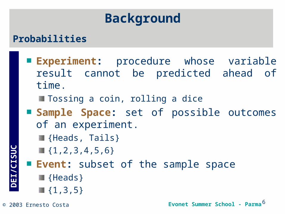
Background

Probabilities

Experiment: procedure whose variable result cannot be predicted ahead of time.

Tossing a coin, rolling a dice

Sample Space: set of possible outcomes of an experiment.

{Heads, Tails}

{1,2,3,4,5,6}

Event: subset of the sample space{Heads}

{1,3,5}

7

DE

I/C

ISU

C


Background

Probability of an EventMeasure the likelihod that the event will occur

Tossing a (fair) coin: probability(outcome=heads) =1/2

AxiomsP(E)0

P(S)=1

For mutually exclusive events

11

( )i iii

P E P E

Probabilities

8

DE

I/C

ISU

C


1/6

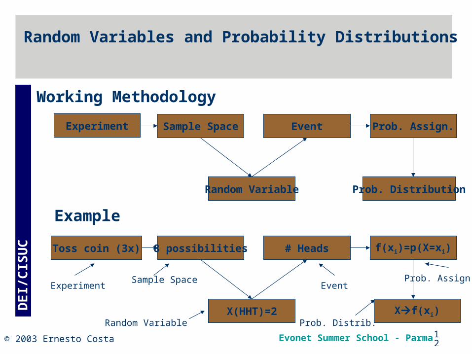
Experiment Prob. Assign.Sample Space Event

ExampleWhat is the probability of when rolling two dice the sum of the two outcomes equal 7?

Working Methodology

Two Dice Experiment

02468

1 2 3 4 5 6 7 8 9 101112

Sum

Nu

mb

er

Tw o DiceExperiment

Background

Probabilities

9

DE

I/C

ISU

C


Definition: Let E and F be two events, with p(F)>0. The conditional probability of E given F, p(E|F), is defined as:

p(E | F) p(EF)

p(F)

Probabilities

Example: A family has two children. Knowing that one is a boy whatis the probability that they have two boys?

1/3

10

DE

I/C

ISU

C


Probabilities

Theorem of Bayes:

)()|()()|(

)()|(

)(

)()|()|1(

2211

1111

ApABpApABp

ApABp

Bp

ApABpBAp

Example: A building has two lifts. One is used by 45% of the residents And the other by 55%. The first one, 5% of the time have problems, whileThe second 8% of the time can let you in trouble. Knowing that one lift had a problem , what is the probability of being lift number 1?

33,8%

11

DE

I/C

ISU

C


Random Variables

Definition: A random variable, X, is a function from the sample space of an experiment to the set of real numbers.

X(s)

s

SX

0 1 2 3

SX

A RV is a function … and is not random!!!

Random Variables and Probability Distributions

12

DE

I/C

ISU

C


Experiment Prob. Assign.Sample Space Event

Random Variable Prob. Distribution

Working Methodology


Toss coin (3x) f(xi)=p(X=xi)8 possibilities # Heads

X(HHT)=2 Xf(xi)

ExperimentSample Space

Random Variable

Event

Prob. Distrib.

Example

Prob. Assign.

13

DE

I/C

ISU

C


Example: Suppose you toss a coin three times. Let X(t) denote the number of heads that appear when t is the result. Então X(t):

X(HHH) = 3X(HHT) = X(HTH) = X(THH) = 2X(TTH) = X(THT) = X(HTT) = 1X(TTT) = 0

Probability Distribution

00,05

0,1

0,150,2

0,250,3

0,350,4

0 1 2 3

X

f(x

i)


Probabilty Distribution

14

DE

I/C

ISU

C



DiscreteProbability Mass Function

ContinuousProbability Density Function (pdf)

( ) ( ) 0P X x p x

Types of Random Variables

( ) 1x

p x

( ) 0,f x x

( ) 1f x dx

( ) ( )b

a

P a X b f x dx x

f(x)

0 x1 x2

15

DE

I/C

ISU

C


LocationMean

DispersionVariance

Standard Deviation

( ) ( )x

E X xp x


Measures of Random Variables

( ) ( )E X xf x dx

2 2( ) ( ) ( )x

V X x p x

2 2( ) ( ) ( )V X x f x

( )V X

16

DE

I/C

ISU

C


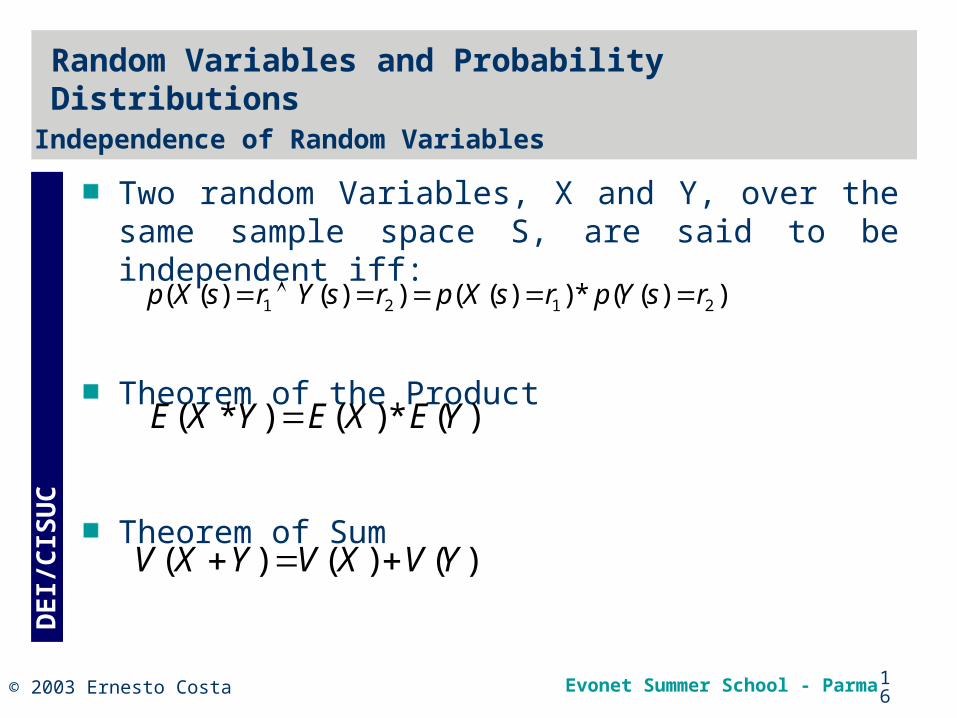
Two random Variables, X and Y, over the same sample space S, are said to be independent iff:

Theorem of the Product

Theorem of Sum

1 2 1 2( ( ) ( ) ) ( ( ) )* ( ( ) )p X s r Y s r p X s r p Y s r


Independence of Random Variables

( ) ( ) ( )V X Y V X V Y

( * ) ( )* ( )E X Y E X E Y

17

DE

I/C

ISU

C



Binomial DistributionDomain {0,1,2,…n}

Probability mass function

Mean np

Variance npq

ininiii qpCpxXp )(

Discrete Probability Distributions

Binomial Distribution

0

0,05

0,1

0,15

0,2

0,25

0,3

1 2 3 4 5 6 7 8 9 10 11 12

Values x

Pro

ba

bili

ty

Series1

Binomial Distribution

0

0,05

0,1

0,15

0,2

0,25

1 2 3 4 5 6 7 8 9 10 11 12

Values x

Pro

babi

lity

Series1

P=0.3 P=0.5

n

i

inini npiqpCXE

0

)(

npqXEXEXV 222 )()()(

18

DE

I/C

ISU

C


Poisson DistributionApproach the Binomial DistributionDomain {0,1,2,3,...}Probability mass functionMean: Variance:

!)(

i

epiXp

i

i


Discrete Probability Distributions

=np Poisson distribution

0

0,05

0,1

0,15

0,2

1 2 3 4 5 6 7 8 9 10 11 12

Values

Pro

ba

bili

ty

Series1

=6Poisson Distribution

00,020,04

0,060,08

0,10,12

0,140,16

1 2 3 4 5 6 7 8 9 10 11 12

Values

Pro

ba

bili

ty

Series1

=8,4

19

DE

I/C

ISU

C


-3 -2 -1 1 2 3

0.1

0.2

0.3

0.4

Normal (Gaussian) Distribution

Standard Normal Distribution


(3,2)N

2

2

2

)(

2

1)(

x

exf

)1,0(N

Continuous Probability Distributions

-4 -2 2 4 6 8 10

0.05

0.1

0.15

0.2

0.25

20

DE

I/C

ISU

C


Converting a normal distribution to a standard normal distribution

X a random Variable withMean Standard Deviation σ

Using a translationDefining a new Random variable

XZ



21

DE

I/C

ISU

C


-3 -2 -1 1 2 3

0.1

0.2

0.3

0.4N(0,1)

=1=5

=101

2

2

1( )

1( , )2 2

f xx

B

Student’s t-DistributionApproximates the standard normal distribution N(0,1)

Degrees of freedom (df),

Mean 0, Variance



22

DE

I/C

ISU

C


Goal: to apply probability theory to data analysis

How?Model the data (population) by mean of a probability distribution

Use a sample of the data instead of the all populationEstimate the population parameters (, σ, p) using correspondent sample statistics (x, s, )

StatisticsBackground

population sample

σ

p

x

sparameters statistics

p̂

p̂

23

DE

I/C

ISU

C


Unbiased estimatorA statistics with mean value equal to the population parameter being estimated

Point Estimators

Interval Estimators

BackgroundStatistics

24

DE

I/C

ISU

C


Background

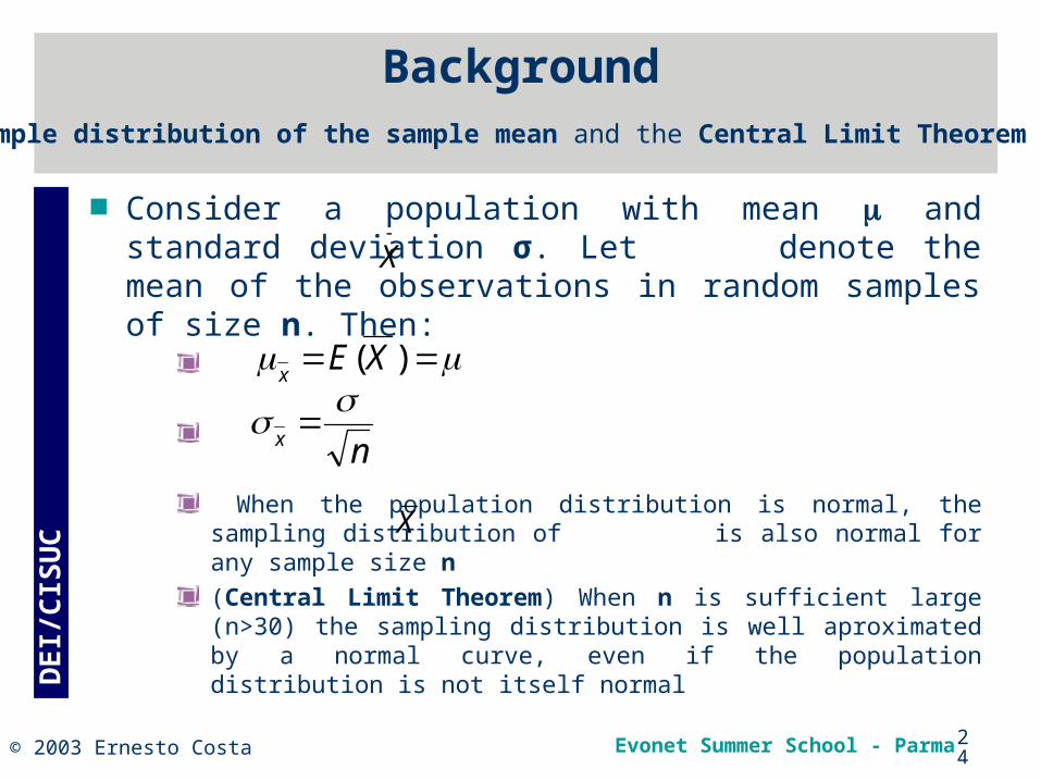
Consider a population with mean and standard deviation σ. Let denote the mean of the observations in random samples of size n. Then:

When the population distribution is normal, the sampling distribution of is also normal for any sample size n

(Central Limit Theorem) When n is sufficient large (n>30) the sampling distribution is well aproximated by a normal curve, even if the population distribution is not itself normal

)(XEx

Sample distribution of the sample mean and the Central Limit Theorem

X

nx

X

25

DE

I/C

ISU

C


Background

Unbiased estimatorsMean

Standard Deviation

)(XEx

Sample distribution of the sample mean

2( )ˆ

1

ii

x

x xs

n

(n-1) are the degrees of freedom (df)

26

DE

I/C

ISU

C


Background

ConsequenceFor a large sample or population whose distribution is normal:

has (approximately) a standard normal (Z) distribution.

Sample distribution of the sample mean and the Central Limit Theorem

x

x

XZ

27

DE

I/C

ISU

C


Background

Estimate the mean The population standard deviation, σ, is known;

The sample mean from a random sample, is known,

The sample size is large (>30)

The one sample Z confidence interval is

Example: for an 95% confidence interval Z=1.96.

X

Confidence Intervals – one sample

_critical valuex Zn

28

DE

I/C

ISU

C


Background

Example: we want a confidence level of 90%Look into a N(0,1)

For a CL of 90%, we have to isolate the area of 5% to the left and to the right of the bell shaped normal distribution.

The confidence interval will be given by

Looking in a table for the value of Z we obtain Z=1.65


0.1

2

x Zn

29

DE

I/C

ISU

C


Background

What does it means having a confidence interval of 95%?

That there is a probability of 95% that the true mean (population) is in the interval? NO!!

Mean that 95% of all possible samples result in an interval that includes the true mean!


30

DE

I/C

ISU

C


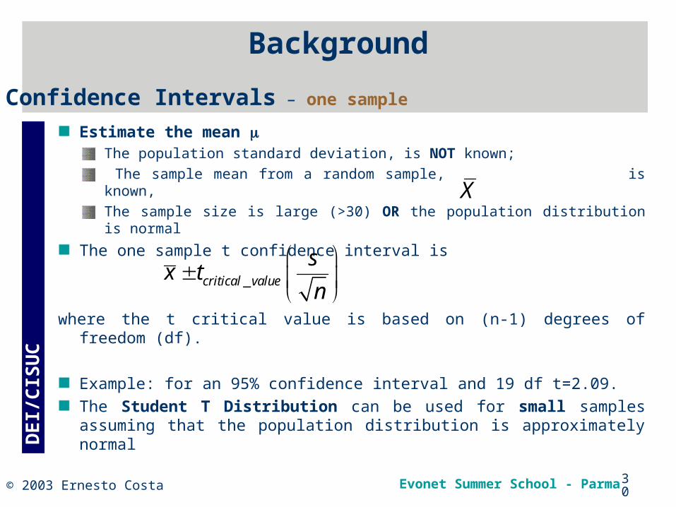
Background

Estimate the mean The population standard deviation, is NOT known;

The sample mean from a random sample, is known,

The sample size is large (>30) OR the population distribution is normal

The one sample t confidence interval is

where the t critical value is based on (n-1) degrees of freedom (df).

Example: for an 95% confidence interval and 19 df t=2.09.

The Student T Distribution can be used for small samples assuming that the population distribution is approximately normal

_critical value

sx t

n


X

31

DE

I/C

ISU

C


Background

A hypothesis is a claim about the value of one or more population characteristics.A test procedure is a method for using sample data to decide between to competing claims about population characteristics. (= 100 or 100)Method by contradiction: we assume a particular hypothesis. Using the sample data we try to find out if there is convincing evidence to reject this hypothesis in favor of a competing one

Hypothesis Testing – one sample

32

DE

I/C

ISU

C


Background

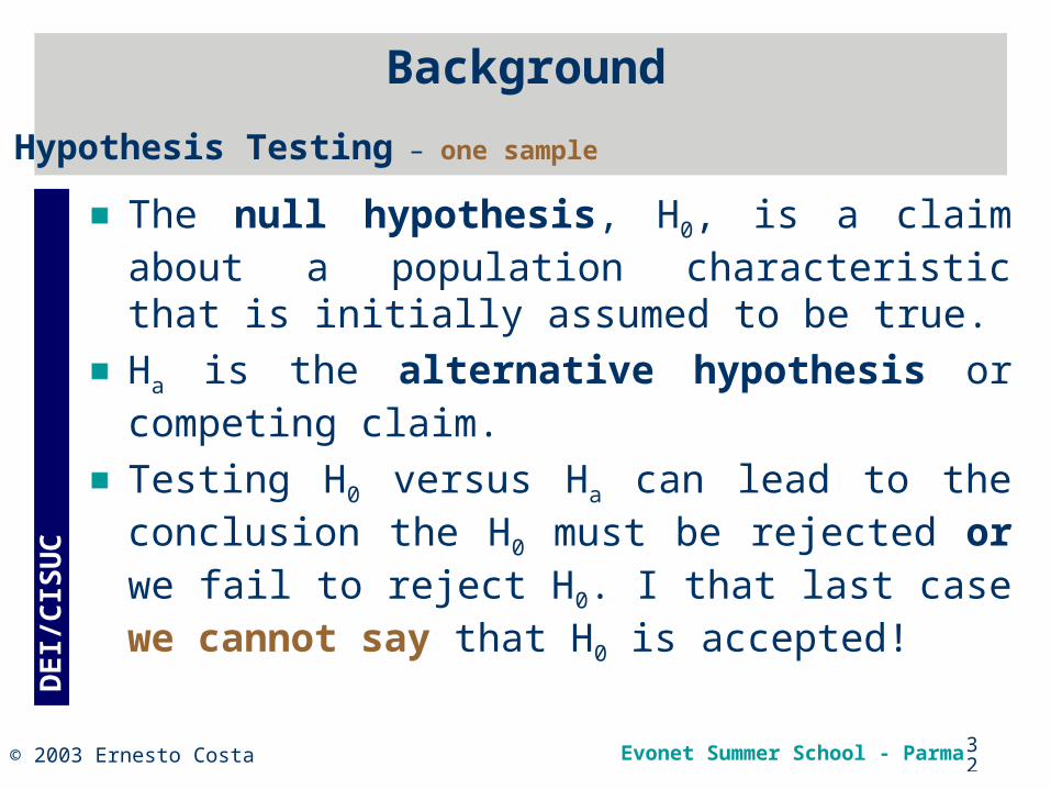
The null hypothesis, H0, is a claim about a population characteristic that is initially assumed to be true.

Ha is the alternative hypothesis or competing claim.

Testing H0 versus Ha can lead to the conclusion the H0 must be rejected or we fail to reject H0. I that last case we cannot say that H0 is accepted!


33

DE

I/C

ISU

C


Background

ErrorsType I error

Rejecting H0 when H0 is true

The probability of a type I error, , is called Level of Significance of the test.

Type II errorFailing to reject H0 when H0 is false

The probability of a Type II error is denoted by .

There is a tradeoff between and : making type I error very small increase the probability of type II error.


34

DE

I/C

ISU

C


Background

Test Statistic (Z,t): function of the sample data on which a decision about reject or fail to reject H0 is based;

p-value (observed significance level): is the probability, assuming that H0 is true, of obtaining a test statistics at least as inconsistent with H0 as what actually resulted.

Decision about H0: comparing the p-value with the chosen .

Reject H0 if p-value


35

DE

I/C

ISU

C


Background

Hypothesis Testing – principlesWhat is the population parameter (mean,…)

State the H0 and Ha

Define the significance level The assumptions for the test are reasonable (big sample,…)

Calculate the test statistic (Z,…)

Calculate the associated p-value

State the conclusion (reject if p-value ,…)


36

DE

I/C

ISU

C


Background

ExamplePopulation parameter the mean, H0: =100, Ha: 100

Significance level =0.01

n=40 is large

From the sample: =105,3, σ=8.4

From the z-curve we know that the p-value 0

Therefore the null hypothesis, H0, is rejected with a significance level of 0.01.

x


105,3 1003.99

8.4

40

z

37

DE

I/C

ISU

C


Background

Use the sample distribution of the difference of the sample means:

PropertiesThe mean of the difference is equal to the difference of the means

The variance of the difference is equal to the sum of the individuals variances. Thus, the standard deviation:

The sampling distribution of the difference of the sample means, can be considered approximately normal (each n large, each sample mean come from a population (approximately) normal

1 2x x

Comparing Two Populations based on independent samples

1 2 1 2x x

1 2

2 2

1 2

1 2x x n n

38

DE

I/C

ISU

C


Background

AssumptionsThe two samples are independently random samples

Sample sizes are both large (n >30) OR the population distributions are (approximately) normal.

Formulas

1 2 1 2x x Confidence interval for the mean of

2 2

1 21 2 _

1 2critical valuex x t

n ns s

2 22

1 2 1 21 22 2

1 21 2

1 21 1

V Vdf where V V

n n

n n

s sV V

39

DE

I/C

ISU

C


Background

Same procedure, only the formulas are different!

Z TestLarge samples OR

Population distributions are (at least approximately) normal

Hypothesis Test

1 2 1 2

2 2

1 2

1 2

( )x xz

n n

40

DE

I/C

ISU

C


Background

t testLarge samples OR

Population distributions normal AND the random samples are independent

1 2 1 2

2 2

1 2

1 2

( )x xt

n ns s

Hypothesis Test

2 22

1 2 1 21 22 2

1 21 2

1 21 1

V Vdf where V V

n n

n n

s sV V

41

DE

I/C

ISU

C


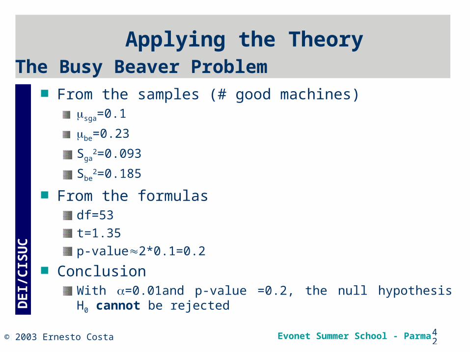
Applying the Theory

Two algorithmsA standard GA

A standard GA + local learning (Baldwin Effect)

Goal: good quality machines

Who is better? Comparing the means!H0:1= 2 (no improvement!!!), Ha: 1≠ 2

Confidence level, =0.01

Assuming that the population distributions are normal

Number of (independent) runs = 30 for each case

Use t test

The Busy Beaver Problem

42

DE

I/C

ISU

C


From the samples (# good machines)sga=0.1

be=0.23

Sga2=0.093

Sbe2=0.185

From the formulasdf=53

t=1.35

p-value2*0.1=0.2

Conclusion With =0.01and p-value =0.2, the null hypothesis H0 cannot be rejected

The Busy Beaver Problem

Applying the Theory

43

DE

I/C

ISU

C


Applying the Theory

Two different GAs applied to function optimization

A standard GA using a 2 point CXover

A modified GA using transformation

Goal: find the minimum

-500

-250

0

250

500 -500

-250

0

250

500

0

500

1000

1500

-500

-250

0

250

500

Function Optimization

The Schwefel Function

Minimum = 0

44

DE

I/C

ISU

C


Who is better? Two point Crossover or Transformation?

Comparing the means of the best fit!

H0:1= 2 (no improvement!!!), Ha: 1≠ 2

Confidence level, =0.05

Assuming the population distributions are normal

Number of (independent) runs = 30 for each case

Use t test

Applying the TheoryFunction Optimization

45

DE

I/C

ISU

C


From the samples (fitness of the best individuals)sga=5.4838

tr=0.0768

Sga2=149.788

Str2=0.02958

From the formulasdf=29

t=2.42

p-value2*0.012=0.024

Conclusion With =0.05 and p-value =0.024, the null hypothesis H0 is rejected.

Applying the TheoryFunction Optimization

46

DE

I/C

ISU

C


Conclusions

This is a very simple presentationAssuming Normal distributions

There are many others

In many situations we cannot assume a normal distribution

Many things left unmentionedMore than two populations

Analysis of Variance (ANOVA)

Regression and Correlation

Non parametric methods

47

DE

I/C

ISU

C


Want to know more?

Paul Cohen, Empirical Methods for Artificial Intelligence. MIT Press, Boston, 1995 James Kennedy and Russell Eberhart, Swarm Intelligence (Appendix A),Morgan Kaufman, 2001.Roxy Peck, Chris Olsen and Jay Devore, Introduction to Statistics and Data Analysis,Duxbury, 2001.Mark Wineberg and Steffen Christensen, Using Appropriate Statistics, GECCO’2003 Tutorial.

dei/cisuc evonet summer school - parma © 2003 ernesto costa 1 how to conduct good experiments?...

Documents

ernesto costa deicisuc

background probability

probabilities example

exclusive events probabilities

conditional probability

dice sample space

random variables definition

probabilities theorem