deform’06 - proceedings of the workshop on image

HAL Id: hal-00094749https://hal.archives-ouvertes.fr/hal-00094749

Submitted on 14 Sep 2006

HAL is a multi-disciplinary open accessarchive for the deposit and dissemination of sci-entific research documents, whether they are pub-lished or not. The documents may come fromteaching and research institutions in France orabroad, or from public or private research centers.

L’archive ouverte pluridisciplinaire HAL, estdestinée au dépôt et à la diffusion de documentsscientifiques de niveau recherche, publiés ou non,émanant des établissements d’enseignement et derecherche français ou étrangers, des laboratoirespublics ou privés.

DEFORM’06 - Proceedings of the Workshop on ImageRegistration in Deformable Environments

Adrien Bartoli, Nassir Navab, Vincent Lepetit

To cite this version:Adrien Bartoli, Nassir Navab, Vincent Lepetit. DEFORM’06 - Proceedings of the Workshop on ImageRegistration in Deformable Environments. Pas d’éditeur commercial, pp.87, 2006. hal-00094749

https://hal.archives-ouvertes.fr/hal-00094749

https://hal.archives-ouvertes.fr

Adrien BartoliNassir NavabVincent Lepetit (Eds.)

Proceedings

DEFORM’06 is associated to BMVC’06, the 7th British Machine Vision Conference

DEFORM’06Workshop on Image Registration in Deformable Environments8 September 2006, Edinburgh, UK

Preface

These are the proceedings of DEFORM’06, the Workshop on Image Registration in Deformable Environments, associated to BMVC’06, the 17th British Machine Vision Conference, held in Edinburgh, UK, in September 2006.

The goal of DEFORM’06 was to bring together people from different domains having interests in deformable image registration.

In response to our Call for Papers, we received 17 submissions and selected 8 for oral presentation at the workshop. In addition to the regular papers, Andrew Fitzgibbon from Microsoft Research Cambridge gave an invited talk at the workshop.

The conference website including online proceedings remains open, seehttp://comsee.univ-bpclermont.fr/events/DEFORM06.

We would like to thank the BMVC’06 co-chairs, Mike Chantler, Manuel Trucco and especially Bob Fisher for is great help in the local arrangements, Andrew Fitzgibbon, and the Programme Committee members who provided insightful reviews of the submitted papers. Special thanks go to Marc Richetin, head of the CNRS Research Federation TIMS, which sponsored the workshop.

August 2006

Adrien BartoliNassir Navab

Vincent Lepetit

General Co-Chairs Adrien Bartoli LASMEA – CNRS / University Clermont II, France

Nassir Navab Technical University of Munich, Germany

Vincent Lepetit EPFL, Lausanne, Switzerland

Lourdes Agapito Queen Mary, University of London, UK

Amir Amini University of Louisville, USA

Fred Azar Siemens Corporate Research, Princeton, USA

Marie-Odile Berger INRIA, Nancy, France

Tim Cootes University of Manchester, UK

Eric Marchand INRIA, Rennes, France

Andrew Davison Imperial College London, UK

Pascal Fua EPFL, Lausanne, Switzerland

Fredrik Kahl Lund Institute of Technology, Sweden

Ali Khamene Siemens Corporate Research, Princeton, USA

Daniel Rueckert Imperial College London, UK

Laurent Sarry University Clermont I, France

Peter Sturm INRIA, Grenoble, France

Nikos Paragios Ecole Centrale de Paris, France

Xavier Pennec INRIA, Sophia-Antipolis, France

Luc Van Gool ETH Zurich, Switzerland and University of Leuven, Belgium

René Vidal Johns Hopkins University, Baltimore, USA

Xavier Lladó Queen Mary, University of London, UK

Julien Pilet EPFL, Lausanne, Switzerland

Christophe Tilmant University Clermont II, France

Geert Willems University of Leuven, Belgium

Vincent Gay-Bellile LASMEA – CNRS / University Clermont II, France

Martin Horn Technical University of Munich, Germany

Mathieu Perriollat LASMEA – CNRS / University Clermont II, France

Programme Committee

Additional Reviewers

Website, Design and Proceedings

Sponsoring Institution

Organization

TIMS is a CNRS Research Federation in Clermont-Ferrand, France

Table of Contents

Using Subdivision Surfaces for 3-D Reconstruction from Noisy Data

The Morphlet Transform: A Multiscale Representation for Diffeomorphisms

Intensity-Unbiased Force Computation for Variational Motion Estimation

GPU Implementation of Deformable Pattern Recognition Using Prototype-Parallel Displacement Computation

Yoshiki Mizukami, Katsumi Tadamura 71

Darko Zikic, Ali Khamene, Nassir Navab 61

Non-linear Registration Between 3D Images Including Rigid Objects: Application to CT and PET Lung Images With Tumors

Antonio Moreno, Gaspar Delso, Oscar Camara, Isabelle Bloch 31

Jonathan R. Kaplan, David L. Donoho 21

A Single Directrix Quasi-Minimal Model for Paper-Like Surfaces

Mathieu Perriollat, Adrien Bartoli 11

Slobodan Ilić 1

Evaluation of a Rigidity Penalty Term for Nonrigid Registration

Marius Staring, Stefan Klein, Josien P.W. Pluim 41

The Constrained Distance Transform: Interactive Atlas Registration With Large Deformations Through Constrained Distances

Bill Hill, Richard A. Baldock 51

Regular Papers

Algorithms for Nonrigid Factorization

Andrew W. Fitzgibbon 81

Invited Talk

Using Subdivision Surfaces for 3–DReconstruction from Noisy Data

Slobodan IlicDeutsche Telekom Laboratories

Ernst-Reuter-Platz 7, 10587 Berlin, [email protected]

Abstract

In this work, we developed a method which effectively uses subdivision sur-faces to fit deformable models to noisy 3–D data. The subdivision modelsprovide a compact low dimensional representation of model parameter space.They also allow a free form deformation of the objects of arbitrary geometry.These two properties make them ideal for fitting deformable models to noisydata.

We tested our approach on stereo data acquired from uncalibrated monoc-ular video sequences, then on data acquired from low qualitylaser scans, andcompared them. We have shown that it can be successfully usedto recon-struct human faces as well as the other 3D objects of arbitrary geometry.

1 Introduction

The subdivision surfaces are very popular approach for smooth surface representation.They has been extensively used in Computer Graphics for geometric modeling, and com-puter animation [15, 12, 4]. The problem of 3D reconstruction from unorganized datapoints using the subdivision surfaces has also been addressed by the graphics commu-nity [7, 9, 11, 14, 2, 8]. Those methods use noise free data produced by high quality laserscanners. In Computer Vision the 3D shapes were extracted from the images which in-volve very noisy information. Since this problem is highly under-constrained, the genericmodels were extensively used [6, 13, 1] to constrain the solution of the reconstructiontask. The main challenge is to find a suitable model parameterization where the numberof parameters is small compared to the overall dimensionality of the problem. On theother hand the parameterization has to support a full free form deformation of the tar-get surface. The subdivision surfaces naturally possess those properties. They produce asmooth mesh from a coarse one as shown in Fig. 2. The initial coarse mesh,control mesh,is a very rough representation of the object of interest. It can be of arbitrary topology, andsubdivision can be appliedN times to it. The final smooth mesh,model mesh, entirelydepends on the initial control mesh. Its shape can be modifiedin a free form manner.Also, the number of control mesh vertices is far smaller thanthe number of actual modelvertices. In this paper we develop a method which relays on subdivision surface modelsto reconstruct 3D objects from noisy data shown in Fig. 1 as opposed to clean laser scandata used in Computer Graphics. We are not aware of any other method which uses sub-division surfaces for 3D shape recovery from nosy data. Besides valuable properties suchas free form deformation and low dimensionality, subdivision models, allowed us to usethe initial control mesh as a regularizer in our optimization framework.

Proceedings of the Workshop on Image Registration in Deformable Environments, Edinburgh, UK, Sept. 2006

Page 1

(a)

(b)

Figure 1: Reconstruction of 3D objects from noisy data: (a) 3–D data clouds correspond-ing to stereo and laser scans respectively. First two imageson the left side are stereodata clouds obtained from uncalibrated, Fig 5, and calibrated, Fig 6, image sequencesrespectively, while the other two correspond to the laser scans.(b) Reconstruction resultsobtained by fitting generic subdivision models to the data from (a). For faces a genericface model was used, while for the frog model is extracted from the scan.

We chose to demonstrate and evaluate our technique mainly inthe context of face-modeling from uncalibrated and calibrated images sequences and from the laser scandata. We compare the recovered models from images to those ofthe laser scans in orderto verify the quality of the reconstruction. To demonstratethat our method can be appliedto objects of different geometry we reconstructed a ceramicstatue of the frog from itslaser scan. The data we are dealing with are noisy and incompletge as it can be seen inFig 1(a), and, yet, we obtained realistic models, whose geometry is correct, as depicted inFig. 1(b).

According to these experiments we argue that the approach isgeneric and can beapplied to any task for which deformable facetized models exist. We therefore view ourcontribution as the integration of a powerful shape representation technique into a robustleast-squares framework.

In the remainder of the paper, we first describe subdivision parameterization in moredetails. We then introduce our least-squares optimizationframework and, finally, presentresults using laser scanned data, calibrated and uncalibrated image sequences.

2 Subdivision Surface Parameterization

The key property of subdivision models is that the smooth high resolution mesh modelsare represented by very coarse initial control mesh. The control mesh consists of rela-tively small number of vertices and completely controls theshape of the smooth meshmodel. The model mesh is obtained by subsequent subdivisionof the initial coarse meshas depicted in Fig. 2.


Page 2

(a)

(b)

Figure 2: Generic models and their subdivisions. (a) The first image on the left corre-sponds to the average face model of [1]. The next image shows the actual control meshwe use. It is obtained by reducing the average face model for 98.8% decreasing numberof vertices from 53235 to only 773. The following images represent model meshes cor-responding to one and two levels of subdivision. The last image is just shaded versionof two times subdivided control mesh. (b) Now, the first imageon the left correspondsto the laser scan of the ceramic frog statue. Following images represent control mesh,model mesh with one and two levels of subdivision and two times subdivided controlmesh shown as shaded.

Our method requires a generic model of the object we want to reconstruct. To quicklyproduce those models we take advantage of the property of thesubdivision that it can beapplied to meshes of arbitrary geometry and topology. Thus,the generic control mesh canbe quickly extracted from already existing high quality generic models or directly formthe data as discussed in Sec. 4 and depicted by Fig. 2.

In the reminder of this section we will review Loop subdivision schema for one levelof subdivision and discuss the hierarchy of subdivision if multiple levels of subdivisionare applied.

2.1 Loop Subdivision

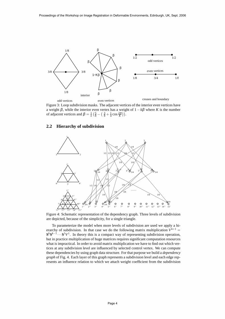
The Loop scheme is a simple approximating face-split schemeapplicable only to trian-gular meshes proposed by Charles Loop [10]. The edge splitting producesodd verticeswhile vertex splitting produceseven vertices. The new vertices areweighted sumof con-trol point neighbors from previous level of subdivision. The weights define subdivisionrules and differ for interior and boundary vertices. These rules can be illustrated by a localmasks called subdivision masks as shown in Fig. 3.

Because of well established rules, the computation of the coefficients and dependen-cies between control and model vertices is straightforward. The coefficients can be as-sembled into a subdivision matrix. Therefore we can parameterize our subdivided meshby control mesh as matrix multiplicationVmod

m×1 = Sm×nVctrln×1, whereSm×n is a subdivision

matrix withm being the number of vertices of subdivided mesh andn number of verticesof control mesh.


Page 3

3/8 3/8

1/8

1/8

β

β

β

β

β

ββ

1−Κβ

1/2 1/2

1/8 3/4 1/8

even vertices

interior

odd vertices even vertices

odd vertices

creases and boundary

Figure 3: Loop subdivision masks. The adjacent vertices of the interior even vertices havea weightβ , while the interior even vertex has a weight of 1−kβ whereK is the numberof adjacent vertices andβ = 1

n

(

58 −

(

38 + 1

4 cos2πK

))

.

2.2 Hierarchy of subdivision

1’’

2’’ 3’’

4’’ 6’’

10’’

11’’ 12’’ 13’’ 14’’ 15’’

6’ 5’ 4’

3 2

1

3’ 2’

1 2 3

1’

7’’ 8’’ 9’’

5’’

3/4

1/21/81/2 1/81/2 1/2

3/4

1/8

5’4’3’2’1’ 6’3/4

1/8

1/81/8

2’’ 3’’ 4’’ 5’’ 6’’ 7’’ 8’’ 9’’ 10’’ 11’’ 12’’ 13’’ 14’’ 15’’1’’3/4

1/8 1/81/2 1/2

1/21/2

3/4

1/8 1/8

1/8

1/8

3/8 3/8..........

3/4

1/8 1/8

Figure 4: Schematic representation of the dependency graph. Three levels of subdivisionare depicted, because of the simplicity, for a single triangle.

To parameterize the model when more levels of subdivision are used we apply a hi-erarchy of subdivision. In that case we do the following matrix multiplication Vk+1 =SkSk−1 · · ·S1V1. In theory this is a compact way of representing subdivisionoperation,but in practice multiplication of huge matrices requires significant computation resourceswhat is impractical. In order to avoid matrix multiplication we have to find out which ver-tices at any subdivision level are influenced by selected control vertex. We can computethese dependencies by using graph data structure. For that purpose we build adependencygraphof Fig. 4. Each layer of this graph represents a subdivision level and each edge rep-resents an influence relation to which we attach weight coefficient from the subdivision


Page 4

masks. In order to find out which vertices are influenced by theselected control vertexwe should propagate all weights at each level. We recursively traverse the graph to findthe influenced vertices. Note that this relation is permanent and has to be computed oncein the beginning.

3 Optimization Framework for Subdivision SurfaceFitting

In this section, we introduce the framework we have developed to fit subdivision surfacesto noisy image data. We fitmesh modelssuch as the ones of Fig. 2 corresponding toseveral levels of subdivision. Our goal is to deform the surface—without changing itstopology—so that it conforms to the image data. The deformation is controled by thecontrol mesh, such as one of Fig. 2. In this work data is made of 3–D points computed us-ing stereo or laser scan data. In standard least-squares fashion, for each point observationxi , we write an observation equation of the formd(xi,S) = εi , whereS is a state vectorcorresponding to the vertices of the control mesh which defines the shape of the surface,d is the distance from the point to the surface andεi is the residual error measuring thedeviation of the data from the model. In practiced(xi ,S) is taken to be the orthonormaldistance ofxi to the closest surface triangulation facet. This results innobsobservationequations forming a vector of residualsF(S) = [ε1, ...,εi , ...]

T1≤i≤nobsthat we minimize in

the least squares sense by minizing its square norm:

χ2 =12

F(S)TWF(S) =nobs

∑i=1

wid(xi ,S)2. (1)

Because some of the observations, may be spurious, we weigh them to eliminateoutliers. Weighting is done as the preprocessing step, before the real fitting is started.Observation weightwi are taken to be inversely proportional to the initial distanced(xi ,S)of the data point to the model surface. More specifically we computewi weight of theobsias:

wi = exp(di

di),1≤ i ≤ nobs (2)

wheredi is the median value of thed(xi,S). In effect, we used(xi ,S) as an estimateof the noise variance and we discount the influence of points that are more than a fewstandard deviations away. Because of the non-differentiability of the distance function werecompute the point to facet attachments before every minimization procedure.

In theory we could take the parameter vectorS to be the vector of allx,y, andzcoordinates of the model mesh. However, because the data we are dealing with are verynoisy and the number of parameters is huge we found that the fitting process to be verybrittle since we deal with very ill-conditioned problem.

3.1 Subdivision parametrization

We therefore use verticescontrol meshsuch as the one of Fig. 2 to be our state vector.More precisely, in our scheme, we take the state vectorSto be the vector of 3-D displace-ments of the control mesh vertices, which is very natural using the subdivision formalism.


Page 5

For each vertex on the model mesh, obtained by several subdivisions of the initial controlmesh, we extract the control vertices and their weights influencing those model veticesusing dependency graph of Fig. 4. This allows us to express displacement of every modelvertexi afterk subdivisions as the weighted linear combination of displacements of con-trol points from previous subdivision levels which influence them as:

Vki = Vnk

i −Vki =

Nck−1

∑ck−1=1

Nck−2

∑ck−2=1

· · ·

Nc0

∑c0=1

wck−1wck−2 · · ·wc0 V0c0

. (3)

whereVnki is the new position after the deformation andVk

i is the initial position of theith model vertex obtained afterk subdivisions. Indicesck− j count number of infulencingcontrol verteces on the previous subdivision levelk− j, j = n,0 wheren is the number ofsubdivision levels. Equally,Nck− j , j = n,0 is the actual number of control vertices on thesubdivision levelk− j influencing the position of theith model vetrex. Weightswck− j areassociated weights from Loop’s subdivision masks of the control vetices on the previoussubdivision level.

(a)

(b)

(c)

(d)

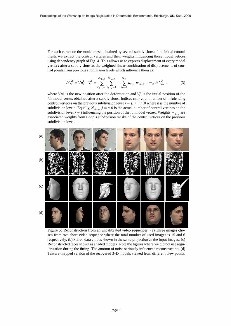
Figure 5: Reconstruction from an uncalibrated video sequences. (a) Three images cho-sen from two short video sequence where the total number of used images is 15 and 6respectively. (b) Stereo data clouds shown in the same projection as the input images. (c)Reconstructed faces shown as shaded models. Note the figureswhere we did not use regu-larization during the fitting. The amount of noise seriouslyinfluenced reconstruction. (d)Texture-mapped version of the recovered 3–D models viewed from different view points.


Page 6

(a)

(b)

Figure 6: Reconstruction from an calibrated video sequence. (a) Five images chosenfrom the calibrated video sequence, courtesy of IGP, ETH Zürich. (b) Reconstructed faceshown as shaded model overlapped on the original image in thesame perspective in orderto highlight the quality of the reconstruction.

3.2 Regularization

Because there are both noise and potential gaps in the image data, we found it necessaryto introduce a regularization term. Since we start with a generic model, we expect thedeformation between the initial shape and the original one to be smooth. This can beeffectively enforced by preventing deformations at neighboring vertices of the controlmesh to be too different. If the control points formed a continuous surface, a naturalchoice would, therefore, be to take this term to be the sum of the square of the derivativesof theV0

i displacements across the initial control mesh. By treatingits facets asC0

finite elements, we can approximate regularization energyED as the quadratic form

ED = λSTKS= λ(

∆txK∆x + ∆t

yK∆y + ∆tzK∆z

)

(4)

whereλ is small regularization constant,K is a very sparse stiffness matrix,S is a statevector containing displacements of along thex,y or z coordinates at each point of thiscontrol surface.

4 Results

We demonstrate and evaluate our technique mainly in the context of face modeling sincemany tools for that are available to us. We show its flexibility also by using it to fit ageneric model of the frog to the noisy scan data.

4.1 Reconstruction from Image Sequences

We recover faces from uncalibrated sequances of Fig. 5(a) and calibrated one of Fig. 6(a)sequences. In the first row of Fig. 5(a) we choose to show threeimages from two differentuncalibrated video sequences. In both cases, we had no calibration information about thecamera or its motion. We therefore used a model-driven bundle-adjustment technique [6]to compute the relative motion and, thus, register the images. We then used the tech-nique [5] to derive the clouds of 3–D points depicted by Fig. 5(b). Because we used fewerimages and an automated self-calibration procedure as opposed to a sophisticated manual


Page 7

0

0.2

0.4

0.6

0.8

1

0 2 4 6 8 10

Pro

port

ion

of th

e sc

an p

oint

s w

ithin

dis

tanc

e

Distance of the laser scan points from the model reconstructed from images in mm

Distance distribution of the laser scan points

0

0.2

0.4

0.6

0.8

1

0 2 4 6 8 10

Pro

port

ion

of th

e sc

an p

oint

s w

ithin

dis

tanc

e

Distance of the laser scan points from the model reconstructed from images in mm

Distance distribution of the laser scan points

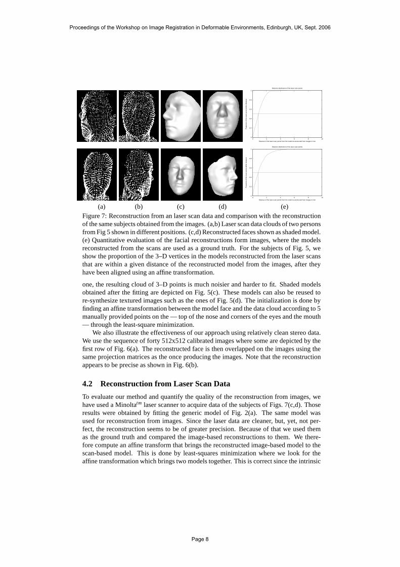
(a) (b) (c) (d) (e)Figure 7: Reconstruction from an laser scan data and comparison with the reconstructionof the same subjects obtained from the images. (a,b) Laser scan data clouds of two personsfrom Fig 5 shown in different positions. (c,d) Reconstructed faces shown as shaded model.(e) Quantitative evaluation of the facial reconstructionsform images, where the modelsreconstructed from the scans are used as a ground truth. For the subjects of Fig. 5, weshow the proportion of the 3–D vertices in the models reconstructed from the laser scansthat are within a given distance of the reconstructed model from the images, after theyhave been aligned using an affine transformation.

one, the resulting cloud of 3–D points is much noisier and harder to fit. Shaded modelsobtained after the fitting are depicted on Fig. 5(c). These models can also be reused tore-synthesize textured images such as the ones of Fig. 5(d).The initialization is done byfinding an affine transformation between the model face and the data cloud according to 5manually provided points on the — top of the nose and corners of the eyes and the mouth— through the least-square minimization.

We also illustrate the effectiveness of our approach using relatively clean stereo data.We use the sequence of forty 512x512 calibrated images wheresome are depicted by thefirst row of Fig. 6(a). The reconstructed face is then overlapped on the images using thesame projection matrices as the once producing the images. Note that the reconstructionappears to be precise as shown in Fig. 6(b).

4.2 Reconstruction from Laser Scan Data

To evaluate our method and quantify the quality of the reconstruction from images, wehave used a Minoltatm laser scanner to acquire data of the subjects of Figs. 7(c,d). Thoseresults were obtained by fitting the generic model of Fig. 2(a). The same model wasused for reconstruction from images. Since the laser data are cleaner, but, yet, not per-fect, the reconstruction seems to be of greater precision. Because of that we used themas the ground truth and compared the image-based reconstructions to them. We there-fore compute an affine transform that brings the reconstructed image-based model to thescan-based model. This is done by least-squares minimization where we look for theaffine transformation which brings two models together. This is correct since the intrinsic


Page 8

(a)

(b)

Figure 8: Reconstruction of the laser scanned frog statue. (a) Laser scan data shownin different position indicating holes and ambiguous partscoming from stitching of theindividual scans. (b) Reconstructed frog model shown in similar positions as the scan.Note, that the holes are filled and the noise is smoothed out.

camera parameters are given the approximate values during bundle-adjustment procedure.This resulted in stereo reconstruction precise up to the affine transformation. In Fig. 7(e),we plot for both subjects, the proportion of the 3–D verticesof the laser-based recoveredmodel that are within a given distance of the image-based reconstructed model, after ithas been deformed using the affine transform discussed above. The median distancesare 0.833858mmand 0.815620mmrespectively. Comparing the reconstruction from im-ages to the original laser scan data gives the increase of themedian error to 1.94mmand2.28mmrespectively. This is normal since the original laser scan data are noisy in contrastto the model fitted to it and used as ground truth in Fig 7.

Our scanner has a theoretical precision of around 0.3mm. However, this does not takeinto account some of the artifacts it produces, such as thosethat occur when stitchingtogether several scans of the target object seen from different viewpoints. A median dis-tance between two independent reconstructions being under1.0mm is therefore a goodindication that our results are consistent with each other.Finally, we show the result ofreconstructing the frog from the noisy laser scan. The frog statue is made of smooth ce-ramic material. Since our scanner is static it required the object to be turned and individualscans to be stitched. The specularities on the eyes producedholes in the scan. As it can beseen in the Fig. 8(a) the scan has quite a lot of ambiguities and missing parts what madeit challenging for reconstruction. The results we obtainedare smooth. The ambiguities,such as one back on the left leg are smoothed and the holes on the eyes are filled as shownin Fig. 8(b). In this way we managed to significantly improve the reconstruction from thescan, by simply extracting the model from the scan and then fitting it back to the originaldata.

5 Conclusion

In this work, we proposed to use the subdivision surfaces to fit generic surface models tonoisy 3–D image and laser scan data. We demonstrated the effectiveness and robustnessof our technique in the context of face modeling where the generic model was available.We also showed that, in fact, we can model other complex shape, such as frog statue, for


Page 9

which a deformable triangulated model exists.In future work we intend to investigate the possibility of using reverse subdivision

to produce even better generic models out of the available hight quality models. Wealso intend to investigate the use of such models in the context of model-based bundleadjustment where both shape and camera parameters can be extracted simultaneouslyfrom image feature correspondences.

References[1] V. Blanz and T. Vetter. A Morphable Model for The Synthesis of 3–D Faces. InComputer

Graphics, SIGGRAPH Proceedings, pages 187–194, Los Angeles, CA, August 1999.

[2] K.-S. D. Cheng, W. Wang, H. Qin, K.-Y. K. Wong, H. Yang, andY. Liu. Fitting subdivisionsurfaces to unorganized point data using sdm. InPacific Conference on Computer Graphicsand Applications, pages 16–24, 2004.

[3] D. DeCarlo and D. Metaxas. The Integration of Optical Flow and Deformable Models withApplications to Human Face Shape and Motion Estimation. InConference on ComputerVision and Pattern Recognition, pages 231–238, 1996.

[4] T. DeRose, M. Kass, and T. Truong. Subdivision surfaces in character animation. InSIG-GRAPH ’98: Proceedings of the 25th annual conference on Computer graphics and interac-tive techniques, pages 85–94, New York, NY, USA, 1998. ACM Press.

[5] P. Fua. From Multiple Stereo Views to Multiple 3–D Surfaces. International Journal ofComputer Vision, 24(1):19–35, August 1997.

[6] P. Fua. Regularized Bundle-Adjustment to Model Heads from Image Sequences without Cal-ibration Data.International Journal of Computer Vision, 38(2):153–171, July 2000.

[7] Hugues Hoppe, Tony DeRose, Tom Duchamp, John McDonald, and Werner Stuetzle. Surfacereconstruction from unorganized points.Computer Graphics, 26(2):71–78, 1992.

[8] W. K. Jeong and C. H. Kim. Direct reconstruction of displaced subdivision surface fromunorganized points. InPacific Conference on Computer Graphics and Applications, pages160–169, October 2001.

[9] N. Litke, A. Levin, and P. Schröder. Fitting subdivisionsurfaces. InProceedings of theconference on Visualization ’01, pages 319–324. IEEE Computer Society, 2001.

[10] C. Loop. Smooth Subdivision Surfaces Based on Triangles. Master thesis, Department ofMathematics, University of Utah, 1987.

[11] V. Scheib, J. Haber, M. C. Lin, and H.-P. Seidel. Efficient fitting and rendering of largescattered data sets using subdivision surfaces.Computer Graphics Forum, 21(3), 2002.

[12] P. Schroder. Subdivision as a fundamental building block of digital geometry processingalgorithms.Journal of Computational and Applied Mathematics, 149, 2002.

[13] Y. Shan, Z. Liu, and Z. Zhang. Model-Based Bundle Adjustment with Application to FaceModeling. InInternational Conference on Computer Vision, Vancouver, Canada, July 2001.

[14] H. Suzuki, S. Takeuchi, F. Kimura, and T. Kanai. Subdivision surface fitting to a range ofpoints. InPacific Conference on Computer Graphics and Applications, page 158. IEEE Com-puter Society, 1999.

[15] D. Zorin, P. Schröder, A. DeRose, L. Kobbelt, A. Levin, and W. Sweldens. Subdivision formodeling and animation. InSIGGRAPH 2000 Course Notes, 2000.


Page 10

A Single Directrix Quasi-Minimal Modelfor Paper-Like Surfaces

Mathieu Perriollat Adrien Bartoli

LASMEA - CNRS / UBP ¦ Clermont-Ferrand, [email protected], [email protected]

http://comsee.univ-bpclermont.fr

Abstract

We are interested in reconstructing paper-like objects from images. Theseobjects are modeled by developable surfaces and are mathematically well-understood. They are difficult to minimally parameterize since the numberof meaningful parameters is intrinsically dependent on the actual surface.

We propose a quasi-minimal model which self-adapts its set of param-eters to the actual surface. More precisly, a varying number of rules isused jointly with smoothness constraints to bend a flat mesh, generating thesought-after surface.

We propose an algorithm for fitting this model to multiple images by min-imizing the point-based reprojection error. Experimental results are reported,showing that our model fits real images accurately.

1 IntroductionThe behaviour of the real world depends on numerous physical phenomena. This makesgeneral-purpose computer vision a tricky task and motivates the need for prior models ofthe observed structures, e.g. [1, 4, 8, 10]. For instance, a 3D morphable face model makesit possible to recover camera pose from a single face image [1].

This paper focuses on paper-like surfaces. More precisly, we consider paper as an un-stretchable surface with everywhere vanishing Gaussian curvature. This holds if smoothdeformations only occurs. This is mathematically modeled by developable surfaces, asubset of ruled surfaces. Broadly speaking, there are two modeling approaches. The firstone is to describe a continous surface by partial differential equations, parametric or im-plicit functions. The second one is to describe a mesh representing the surface with asfew parameters as possible. The number of parameters must thus adapts to the actualsurface. We follow the second approach since we target at computationally cheap fittingalgorithms for our model.

One of the properties of paper-like surfaces is inextensibility. This is a nonlinearconstraint which is not obvious to apply to meshes, as Figure 1 illustrates. For instance,Salzmann et al. [10] use constant length edges to generate training meshes from which agenerating basis is learnt using Principal Component Analysis. The nonlinear constraintsare re-injected as a penalty in the eventual fitting cost function. The main drawback of thisapproach is that the model does not guarantee that the generated surface is developable.


Page 11

PSfrag replacements

AABB

C

C

C

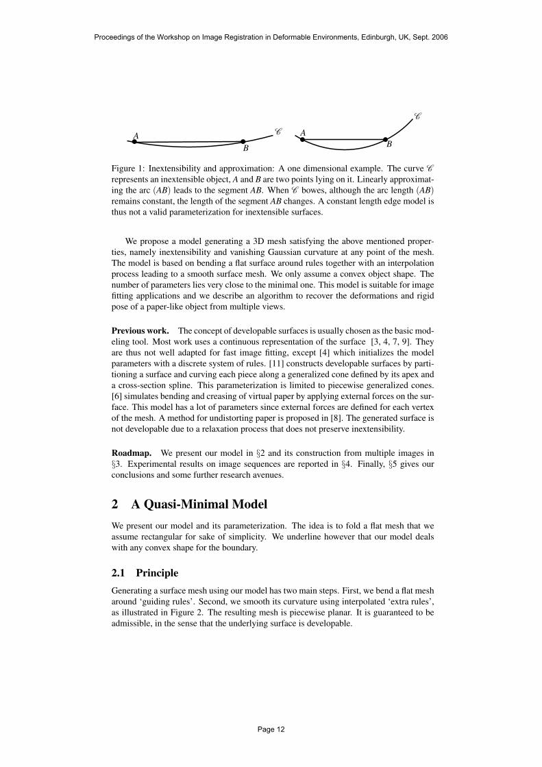
Figure 1: Inextensibility and approximation: A one dimensional example. The curve C

represents an inextensible object, A and B are two points lying on it. Linearly approximat-ing the arc (AB) leads to the segment AB. When C bowes, although the arc length (AB)remains constant, the length of the segment AB changes. A constant length edge model isthus not a valid parameterization for inextensible surfaces.

We propose a model generating a 3D mesh satisfying the above mentioned proper-ties, namely inextensibility and vanishing Gaussian curvature at any point of the mesh.The model is based on bending a flat surface around rules together with an interpolationprocess leading to a smooth surface mesh. We only assume a convex object shape. Thenumber of parameters lies very close to the minimal one. This model is suitable for imagefitting applications and we describe an algorithm to recover the deformations and rigidpose of a paper-like object from multiple views.

Previous work. The concept of developable surfaces is usually chosen as the basic mod-eling tool. Most work uses a continuous representation of the surface [3, 4, 7, 9]. Theyare thus not well adapted for fast image fitting, except [4] which initializes the modelparameters with a discrete system of rules. [11] constructs developable surfaces by parti-tioning a surface and curving each piece along a generalized cone defined by its apex anda cross-section spline. This parameterization is limited to piecewise generalized cones.[6] simulates bending and creasing of virtual paper by applying external forces on the sur-face. This model has a lot of parameters since external forces are defined for each vertexof the mesh. A method for undistorting paper is proposed in [8]. The generated surface isnot developable due to a relaxation process that does not preserve inextensibility.

Roadmap. We present our model in §2 and its construction from multiple images in§3. Experimental results on image sequences are reported in §4. Finally, §5 gives ourconclusions and some further research avenues.

2 A Quasi-Minimal ModelWe present our model and its parameterization. The idea is to fold a flat mesh that weassume rectangular for sake of simplicity. We underline however that our model dealswith any convex shape for the boundary.

2.1 PrincipleGenerating a surface mesh using our model has two main steps. First, we bend a flat mesharound ‘guiding rules’. Second, we smooth its curvature using interpolated ‘extra rules’,as illustrated in Figure 2. The resulting mesh is piecewise planar. It is guaranteed to beadmissible, in the sense that the underlying surface is developable.


Page 12

Step 1: Bending with guiding rules. A ruled surface is defined by a differentiablespace curve α(t) and a vector field β (t), with t in some interval I, see e.g. [11]. Points onthe surface are given by:

X(t,v) = α(t)+ vβ (t) , t ∈ I v ∈ R β (t) 6= 0. (1)

The surface is actually generated by the line pencil (α(t),β (t)). This formulation iscontinuous.

Since our surface is represented by a mesh, we only need a discrete system of rules(sometimes named generatrices), at most one per vertex of the mesh. Keeping all possiblerules leads to a model with a high number of parameters, most of them being redundantdue to surface smoothness. In order to reduce the number of parameters, we use a subsetof rules: The guiding rules. Figure 2 (left) shows the flat mesh representing the surfacewith the selected rules. We associate an angle to each guiding rule and bend the meshalong the guiding rules accordingly. Figure 2 (middle) shows the resulting guiding mesh.The rules are choosen such that they do not to intersect each other, which corresponds tothe modeling of smooth deformations.

Step 2: Smoothing with extra rules. The second step is to smooth the guiding mesh.To this end, we hallucinate extra rules from the guiding ones, thus keeping constant thenumber of model parameters. This is done by interpolating the guiding rules. The foldingangles are then spread between the guiding rules and the extra rules, details are given inthe next section. Figure 2 (right) shows the resulting mesh.

Flat mesh Guiding mesh Smoothed mesh

Figure 2: Surface mesh generation. (left) Flat mesh with guiding rules (in black). (middle)Mesh folded along the guiding rules. (right) Mesh folded along the guiding and extrarules.

2.2 ParameterizationA guiding rule i is defined by its two intersection points Ai and Bi with the mesh boundary.Points Ai and Bi thus have a single degree of freedom each. A minimal parameterizationis their arc length along the boundary space curve. Since the rules do not intersect eachother on the mesh, we define a ‘starting point’ Ps and an ‘ending point’ Pe such that allrules can be sorted from Ps to Pe, as shown on Figure 3 (left). Points Ai (resp. Bi) thushave an increasing (resp. decreasing) arc length parameter. The set of guiding rulesis parameterized by two vectors sA and sB which contain the arc lengths of points Aiand Bi respectively. The non intersecting rules constraint is easily imposed by enforcingmonotonicity on vectors sA and sB.


Page 13

As explained above, the model is smoothed by adding extra rules. This is done byinterpolating the guiding rules. Two piecewise cubic Hermite interpolating polynomialsare computed from the two vectors sA and sB. They are called fA and fB. This interpolationfunction has the property of preserving monotonicity over ranges, as required. Figure 3(right) shows these functions and the control points sA and sB. The bending angles areinterpolated with a spline and rescaled to account for the increasing number of rules.

Pe

Ps

A1

A2A3A4

A5

B5

B4B3 B2 B1 1 2 3 4 5 6 7

0

25

50

75

100

Arc

leng

th Perimeterof thesheet

Rules

Ps

Pe

Pe

A1

A2A3

A4A5

B5B4

B3

B2B1

Figure 3: (left) The generated mesh with the control points (Ai,Bi). (right) Arc lengths sAand sB of the control points with the interpolating functions fA and fB.

Table 1 summarizes the model parameters. The model has 4 + S + 3n parameters, Sbeing the number of parameters describing the mesh boundary (for instance, width andheight in the case of a rectangular shape) and n being the number of guiding rules.

Parameters Description Sizen number of guiding rules 1ne number of extra rules 1S mesh boundary parameters SPs arc length of the ‘starting point’ 1Pe arc length of the ‘ending point’ 1sA arc lengths of the first point defining the guiding rules nsB arc lengths of the second point defining the guiding rules nθ bending angles along the guiding rules n

Table 1: Summary of the model parameters. (top) Discrete parameters (kept fixed duringnonlinear refinement step). (bottom) Continuous parameters.

The deformation is parameterized by the guiding rules. Those are sorted from the‘starting point’ to the ‘ending point’, making wavy the deformation.

We define a directrix as a curve on the surface that crosses some rules once. A min-imal comprehensive set of directrices has the least possible number of directrices suchthat each rule is crossed by exactly one directrix. It is obvious that this set is reduced toa single curve for our model, linking the ‘starting point’ to the ‘ending point’. Conse-quenctly surfaces requiring more than one directrix can not be generated by our model,as for example a sheet with the four corners pulled up. The model however shows to beexperimentally very effective.


Page 14

3 A Multiple View Fitting AlgorithmOur goal is to fit the model to multiple images. We assume that a 3D point set andcamera pose have been reconstructed from image point features by some means. We usethe reprojection error as an optimization criterion. As is usual for dealing with such anonlinear criterion, we compute a suboptimal initialization that we iteratively refine.

3.1 InitializationWe begin by reconstructing a surface interpolating the given 3D points. A rule detectionprocess is then used to infer our model parameters.

Step 1: Interpolating surface reconstruction. Details about how the 3D points arereconstructed are given in §4.1. The interpolating surface is represented by a 2D to 1DThin-Plate Spline function [2], mapping some planar parameterization of the surface topoint height. Defining a regular grid on the image thus allows us to infer the points on the3D surface. Figure 4 and Figure 6 show two examples.

Step 2: Model initialization by rule detection. The model is initialized from the 3Dsurface. The side length is choosen as the size of the 3D mesh.

Guiding rules must be defined on the surface. This set of n rules must represent thesurface as accurately as possible. In [3] an algorithm is proposed to find a rule on agiven surface. It is a method that tries rules on several points on the surface with varyingdirection. We use it to compute rules along sites lying on the diagonal, the horizontal andthe vertical axes. These sites are visible on Figure 4.

Figure 4: Model initialization. (left) Reconstructed 3D points and the interpolating sur-face. (right) Points where rules are sought.

The rules are described by the arc length of their intersection points with the meshboundary. The two arc lengths defining a rule i can be interpreted as a point Ri in R

2,as shown in Figure 5 . Our goal is now to find the vectors sA and sB which define theguiding rules, such that their interpolating functions fA and fB, defining the parametriccurve ( fA, fB) in R

2, describe the rules. We thus compute sA and sB such that the distancebetween the curve ( fA, fB) and the points Ri is minimized. We fix the number of guidingrules by hand, but a model selection approach could be used to determine it from the setof rules.

This gives the n guiding rules. The bending angle vector θ is obtain from the 3Dsurface by assuming it is planar between two consecutive rules. The initial suboptimalmodel we obtain is shown on Figure 6.


Page 15

1 1.5 2 2.5 3 3.5 4−0.5

0

0.5

1

1.5

Arc

leng

th o

f poi

nts

Bi

Arc length of points Ai

PSfrag replacementsArc length

of points Bi

Figure 5: The points in gray represent the detected rules. The black curve is the parametriccurve ( fA, fB) and the black points are the estimated controls points that define the initialrules.

3.2 RefinementThe reprojection error describes how well the model fits the actual data, namely the imagefeature points. We thus introduce latent variables representing the position of each pointonto the modeled mesh with two parameters. Let L be the number of images and N thenumber of points, the reprojection error is:

e =N

∑i=1

L

∑j=1

(m j,i −Π(C j,M(S,xi,yi)))2. (2)

In this equation, m j,i is the i-th feature point in image j, Π(C,M) projects the 3D point Min the camera C and M(S,xi,yi) is a parameterization of the points on the surface, with Sthe surface parameters. The points on the surface are initialized by computing each (xi,yi)such that their individual reprojection error is minimized, using initial surface model.

To minimize the reprojection error, the following parameters are tuned: The parame-ters of the model (the number of guiding and extra rules is fixed), see Table 1, the pose ofthe model (rotation and translation of the generated surface) and the 3D point parameters.

The Levenberg-Marquardt algorithm [5] is used to minimize the reprojection error.Upon convergence, the solution is the Maximum Likelihood Estimate under the assump-tion of an additive i.i.d. Gaussian noise on the image feature points.

4 Experimental ResultsWe demonstrate the representational power of our fitting algorithm on several sets ofimages. First, we present the computation of a 3D point cloud. Second, we show theresults for the three objects we modeled. Third, we propose some augmented realityillustrations.

4.1 3D Points ReconstructionThe 3D point cloud is generated by triangulating point correspondences between severalviews. These correspondences are obtained while recovering camera calibration and poseusing Structure-from-Motion [5]. Points off the object of interest and outliers are removedby hand. Figure 4 shows an example of such a reconstruction.


Page 16

Figure 6: (top) 3D surfaces. (bottom) Reprojection into images. (left) Interpolated sur-face. (middle) Initialized model. (right) Refined model.

4.2 Model FittingEven if our algorithm deals with several views, the following results have been performedwith two views. Figure 6 and Figure 7 show the 3D surfaces, their reprojection into im-ages and the reprojection errors distribution for the paper sequence after the three mainsteps of our algorithm: The reconstruction (left), the initialization (middle) and the refine-ment (right). Although the reconstruction has the lowest reprojection error, the associatedsurface is not satisfying, since it is not enough regular and does not fit the borders of thesheet. The initialization makes the model more regular, but is not enough accurate to fitthe boundary of the paper, so that important reprojection errors remain. At last, the refinedmodel is visually acceptable and its reprojection error is very close to the reconstructedone. It means that our model accurately fits the image points, while being governed bya much lower number of parameters than the set of independant 3D points has. More-over the reprojection error significantly decreases thanks to the refinement step, whichvalidates relevance of this step.

0 0.5 1 1.5 2 2.5 30

5

10

15

20

25

30

35

Reprojection error (pixels)

Num

ber

of p

oint

s

RMS error = 0.737 pixels

0 5 10 15 20 25 30 35 40 450

10

20

30

40

50

60

70

80

90


Num

ber

of p

oint

s


0 0.5 1 1.5 2 2.5 30

5

10

15

20

25

30

35


Num

ber

of p

oint

s


Figure 7: Reprojection errors distribution for the images shown in Figure 6. (left) 3Dpoint cloud. (middle) Initial model. (right) Refined model.

We have tested our method on images of a poster. The results are shown in Figures 8.The reprojections of the computed model are acceptable: The reprojection error of thereconstruction is 0.35 pixels and the one for the refined model is 0.59 pixels.

At last, we fit the model to images of a rug. Such an object does not really sat-isfy the constraints of developable surfaces. Nevertheless, it is stiff enough to be well-


Page 17

Figure 8: Poster mesh reconstruction. (left) Estimated Model. (middle) Reprojection ontothe first image. (right) Reprojection onto the second image.

approximated by our model. The results are thus slightly less accurate than for the paperand the poster: The reprojection error of the reconstruction step is 0.34 pixels and the oneof the final model is 1.36 pixels. Figure 9 shows the reprojection of the model onto theimages used for the reconstruction.

Figure 9: Rug mesh reconstruction. (left) Estimated Model. (middle) Reprojection ontothe first image. (right) Reprojection onto the second image.

4.3 ApplicationsWe demonstrate the proposed model and fitting algorithm by unwarping and augmentingimages, as shown on Figures 10 and 11. Knowing where the paper is projected onto theimages allows us to change the texture map or to overlay some pictures. The augmentingprocess is described in Table 2. Since we estimate the incoming lighting, the augmentedimages look realistic.

AUGMENTING IMAGES

1. Run the proposed algorithm to fit the model to images

2. Unwarp one of the images chosen as the reference one to get the texture map

3. Augment the texture map

4. For each image automatically do

4.1 Estimate lighting change from the reference image

4.2 Transfer the augmented texture map

Table 2: Overview of the augmenting process.


Page 18

Figure 10: Some applications. (left) Unwarped texture map of the paper. (middle) Chang-ing the whole texture map. (right) Augmented paper.

Figure 11: Augmentation. (left) Augmented unwarped texture map. (middle) Augmentedtexture map in the first image. (right) Synthetically generated view of the paper with theaugmented texture map.

5 Conclusion and Future WorkThis paper describes a quasi-minimal model for paper-like objects and its estimation frommultiple images. Although there are few parameters, the generated surface is a goodapproximation of smoothly deformed paper-like objects. This is demonstrated on realimage sequences thanks to a fitting algorithm which initializes the model first and thenrefines it in a bundle adjustment manner.

There are many possibilities for further research. The proposed model could be em-bedded in a monocular tracking framework or used to generate sample meshes for alearning-based model construction.

We currently work on alleviating the model limitations mentioned earlier, namelyhandling a general boundary shape and the comprehensive set of feasible deformation.

References[1] V. Blanz and T. Vetter. Face recognition based on fitting a 3D morphable model.

IEEE Transactions on Pattern Analysis and Machine Intelligence, 25(9), September2003.


Page 19

[2] F. L. Bookstein. Principal warps: Thin-plate splines and the decomposition ofdeformations. IEEE Transactions on Pattern Analysis and Machine Intelligence,11(6):567–585, June 1989.

[3] H.-Y. Chen and H. Pottmann. Approximation by ruled surfaces. Journal of Compu-tational and Applied Mathematics, 102:143–156, 1999.

[4] N. A. Gumerov, A. Zandifar, R. Duraiswami, and L. S. Davis. Structure of appli-cable surfaces from single views. In Proceedings of the European Conference onComputer Vision, 2004.

[5] R. I. Hartley and A. Zisserman. Multiple View Geometry in Computer Vision. Cam-bridge University Press, 2003. Second Edition.

[6] Y. Kergosien, H. Gotoda, and T. Kunii. Bending and creasing virtual paper. IEEEComputer Graphics & Applications, 14(1):40–48, 1994.

[7] S. Leopoldseder and H. Pottmann. Approximation of developable surfaces withcone spline surfaces. Computer-Aided Design, 30:571–582, 1998.

[8] M. Pilu. Undoing page curl distortion using applicable surfaces. In Proceedings ofthe International Conference on Computer Vision and Pattern Recognition, Decem-ber 2001.

[9] H. Pottmann and J. Wallner. Approximation algorithms for developable surfaces.Computer Aided Geometric Design, 16:539–556, 1999.

[10] M. Salzmann, S. Ilic, and P. Fua. Physically valid shape parameterization for monoc-ular 3-D deformable surface tracking. In Proceedings of the British Machine VisionConference, 2005.

[11] M. Sun and E. Fiume. A technique for constructing developable surfaces. In Pro-ceedings of Graphics Interface, pages 176–185, May 1996.


Page 20

The Morphlet Transform: A MultiscaleRepresentation for Diffeomorphisms

Jonathan R. Kaplan, David L. DonohoDept. of Mathematics, Statistics

Stanford UniversityStanford, CA, 94305-2125, [email protected]

Abstract

We describe a multiscale representation for diffeomorphisms. Our rep-resentation allows synthesis – e.g. generate random diffeomorphisms – andanalysis – e.g. identify the scales and locations where the diffeomorphismhas behavior that would be unpredictable based on its coarse-scale behav-ior. Our representation has a forward transform with coefficients that areorganized dyadically, in a way that is familiar from wavelet analysis, and aninverse transform that is nonlinear, and generates true diffeomorphisms whenthe underlying object satisfies a certain sampling condition.

Although both the forward and inverse transforms are nonlinear, it is pos-sible to operate on the coefficients in the same way that one operates onwavelet coefficients; they can be shrunk towards zero, quantized, and canbe randomized; such procedures are useful for denoising, compressing, andstochastic simulation. Observations include: (a) if a template image withedges is morphed by a complex but known transform, compressing the mor-phism is far more effective than compressing the morphed image. (b) Onecan create random morphisms with and desired self-similarity exponents byinverse transforming scaled Gaussian noise. (c) Denoising morpishms in asense smooths the underlying level sets of the object.

1 IntroductionTemporal or spacial deformation is a common underlying source of variability in manysignal and image analysis problems. This deformation may be the result of measurementdistortions, as in the case of satellite imagery [1] and GC/MS data [12] or the deformationmay be the actual phenomenon of study [9, 11]. In the first case, the deformation is seenas a nuisance and must be removed before further analysis. In the second case, the goalis not the removal of the deformation but rather the extraction of the deformation. Oncethe deformation has been extracted, understanding the phenomenon at hand consists ofanalyzing the deformation itself. This paper presents a novel representation for the defor-mation after extraction that takes advantage of smoothness and multiscale organization toboth ease the computational burden of analysis and reveal geometric structure.


Page 21

For the problem of deformation analysis we will limit ourselves to deformations thatare diffeomorphisms–special deformations that are invertible, smooth, and have smoothinverses – this specialization allows us to limit the problem to one that is mathemati-cally amenable. Although they are one of the basic building blocks of modern theoreticalmathematics, and an everyday object in pure mathematics, diffeomorphisms are a newdata type in image and signal analysis. This new data type needs a representation nativeto its own structures. This representation should allow for fast computation and storagewhile maintaining as much transparency as possible. In this paper we present one possibleapproach to addressing this need.

We present a novel nonlinear invertible multiscale transform on the space of diffeo-morphisms that can be used to store, manipulate, and analyze the variability in a collec-tion of signals that are all diffeomorphic to a given template. This multiscale transform isknown as the Morphlet Transform. The use of such a transform is motivated by the suc-cess of multiscale methods in data compression [5], noise removal [4], and fast templateregistration [7]. Many realistic diffeomorphisms that appear in image and signal analysisare sparsely represented in the Morphlet transform space.

There is one chief obstacle to representing diffeomorphisms: the space of diffeomor-phisms is not a linear function space. Diffeomorphisms are functions, and so any givendiffeomorphism may be expressed in a basis expansion. But perturbations or manipula-tions of the expansion coefficients may produce, after reconstruction, a function that is nolonger a diffeomorphism. This will be true regardless of the basis functions that are used.

There are two typical strategies for representing diffeomorphisms. The first is torestrict to a parametric family of functions like affine maps, polynomials, or thin-platesplines. Although these methods are attractive due to their simplicity, with the exceptionof affine maps, none of these methods can guarantee that the matching function is in facta diffeomorphism. The second strategy is to use a deformation vector field such as in [6].The diffeomorphism is then the unit time flow induced by the vector field. The vector fieldrepresentation has three drawbacks: first, calculating features of the full diffeomorphisminvolves solving a first order PDE, which can be computationally intensive; second, therepresentation is global, so the values of the vector field outside of some region can ef-fect the value of the diffeomorphism in the region; third, because of the global nature ofthe vector field the multiscale structure of the field may not correspond to the multiscalestructure of the diffeomorphism. In contrast, the Morphlet transform offers a local andcomputationally efficient description for diffeomorphisms that ensures that the matchingfunctions are, in fact, diffeomorphisms.

The Morphlet transform takes uniform samples of the diffeomorphism on the standardtetrahedral lattice and returns a collection of coefficients indexed by scale and location.These coefficients have the same organizational structure as the coefficients produced bythe wavelet transform. Like the wavelet transform, the Morphlet coefficients reflect thedeviation of the diffeomorphism at one scale and location from the behavior predictedfrom the next coarser scale values. Unlike the wavelet transform, a given coefficient nolonger corresponds to an element of a basis set. Rather, both decomposition and recon-struction are nonlinear.


Page 22

1.1 Related WorkThere is now a long history of the use of multiscale methods in image registration anddeformation [8]. On the question of representing diffeomorphism, D. Mumford and E.Sharon have worked on the question of the conformal fingerprint for conformal diffeo-morphisms between two simply connected regions of the plane [11]. T.F. Cootes et al.[2]work on building a parametric statistical model on the space of diffeomorphisms. A greatdeal of interest in pattern analysis using diffeomorphic registration has been generated inthe field of computational anatomy. See [6, 9].

2 Template Warping and DiffeomorphismsBefore we continue, let us define some terms and make precise the problem we wish toaddress. For our purposes, a diffeomorphism is a smooth function from Rn to Rn whichis one to one, onto, and has a smooth inverse. We shall model signals and images asreal-valued functions on Rn. The deformation of a signal will be the action of a diffeo-morphism on the signal.

Ideform(x) = φ∗(I)(x) = I φ

−1(x). (1)

We assume we have a collection of signals InNn=1 and a fixed template signal Itemplate

such that for each signal In there exists a diffeomorphism φn such that:

In = φ∗n (Itemplate). (2)

We will not address the question of how to calculate φn given In and Itemplate. There isa large existing literature devoted to solving the diffeomorphic registration problem [10],and we postpone discussing the relationship between the morphlet transform and regis-tration algorithms for a later publication. We will simply assume that we can calculate φnsatisfying (2) or some appropriate regularization.1

Once the set of registering diffeomorphisms, φnNn=1, has been obtained, all of the

information contained in the sample InNn=1 is now contained (up to the accuracy of

the diffeomorphic assumption) in the set of registering diffeomorphisms and the templateItemplate. If we want to study the variability of InN

n=1 we need only study the variability ofφnN

n=1. This is advantageous due to the smoothness of the registering diffeomorphisms.Typically, the measured signals are not smooth. In 1-d, the signals may have jumps

and spikes. In 2-d, the images have edges and textures. Representing these features canbe difficult, and most of the science of image analysis focuses on ways of dealing withthese non-smooth features. In contrast, the registering diffeomorphisms are frequentlyvery smooth functions with a few localized regions of sharp transition. These regions ofsharp transition in the registering diffeomorphisms are exactly the regions responsible forthe variability in the collection of signals InN

n=1.Bijections that are smooth except for a few local singularities have sparse Morphlet

transforms. Thus, even when analyzing images with high spatial resolution, only a smallfraction of the morphlet coefficients of the resulting registering diffeomorphisms will belarge. Only these large coefficients are important. Morphlet transform preserves diffeo-morphisms, and has approximation properties similar to the wavelet transform. Thus, if

1In the presence of noise, (2) is never satisfied. Rather, registration algorithms typically search for a diffeo-morphism that satisfies a regularized least squares problem.


Page 23

we threshold and discard small coefficients, the reconstructed diffeomorphism will have asparse representation and will be very close to the original diffeomorphism. We will giveexamples of such a reconstruction in section 5.2.

3 The Interpolating Wavelet TransformsThe Morphlet transform is a nonlinear variant of the wavelet transform. We do not havethe space to give a thorough introduction to the theory of linear wavelet transforms, butbecause the Morphlet transform explicitly builds off of the interpolating wavelet transform[3] we will briefly describe its construction and properties. For ease of presentation wewill only discuss the one dimensional case; the higher dimensional case is similar.

The linear interpolating wavelet transform is defined on the dyadic samples of a con-tinuous real-valued function. Let f be a continuous function on R. Fix integers J0 and J1which will serve as the coarsest and finest dyadic sampling scales respectively. Sample fat k

2J1for k ∈ Z. Define β

jk as:

βj

k = f (k2 j ) (3)

for J0 ≤ j ≤ J1.Fix a positive odd integer D. And define the prediction Pred j

k as:

Pred jk = π

jk (

k2 j +

12 j+1 ), (4)

where πj

k is a local interpolating polynomial of order D. Specifically,

πj

k interpolates the values (k + i2 j ,β j

k+i) for i =−D−12

, . . . ,D+1

2. (5)

We define the linear interpolating wavelet transform as the set of coefficients:β

J0k ,α j,linear

k

j,k∈Z

(6)

whereα

j,lineark = β

j+12k+1−Pred j

k. (7)

Thus, αj,linear

k measures the discrepancy between the true value of the function andthe value predicted by using the samples at the next coarser scale. The coefficients β

J0k

are called the coarse scale coefficients and αj,linear

k are called the detail coefficients. Inregions where f is smooth, the detail coefficients decay exponentially in j. The rate ofdecay measures the degree of smoothness of f . If a function is smooth everywhere exceptfor a few isolated singularities, then the fine scale coefficients of the wavelet transformwill be very small away from the singularities.

To invert the transform we employ a pyramidal scheme starting with the coarsestsample β

J0k . For each scale j, we predict the values at the next finer scale j + 1 using (4)

and reconstruct the samples at scale j +1 using:

βj+1

2k+1 = αj,linear

k +Pred jk. (8)

Both the forward and inverse transforms involve O(N) flops, where N is the number ofsamples of f .


Page 24

4 The Morphlet TransformThe Morphlet transform acts on the dyadic samples of a continuous diffeomorphism ofRn. We will show the 2-d version of the transform, as the simplicity of diffeomorphisms indimension n = 1 makes the 1-d transform insufficiently instructive. The high dimensionalversions follow the same pattern as the 2-d transform.

4.1 The Sampling ConditionDue to a sampling condition, the Morphlet transform is only actually defined for a specialsub-manifold of the space of diffeomorphisms. The idea behind the sampling condition isto ensure, at each scale, that the reconstructed function “looks like a diffeomorphism.” Inparticular, we demand that the discrete Jacobians of the samples of the diffeomorphismare all positively oriented affine maps at all scales. For any given diffeomorphism thereexists a dyadic scale J such that for all scales finer than J the discrete Jacobians satisfythis condition. Thus, a diffeomorphism needs to be sufficiently finely sampled before theMorphlet transform may be applied.

Let φ be a diffeomorphism of the plane. As in the linear case define βj

k,l :

βj

k,l = φ(k2 j ,

l2 j ) (9)

To clarify the sampling condition, and ease the notation for the definition of the fine scalecoefficients, we define three intermediate sets of samples, β

j,0k,l , β

j,1k,l , and β

j,2k,l .

βj,3

k,l = βj

k,l (10)

βj+1,1

2k,2l = βj+1,2

2k,2l = βj,3

k,l (11)

βj+1,1

2k+1,2l+1 = βj+1,2

2k+1,2l+1 =12(β j,3

k+1,l +βj,3

k,l+1) (12)

βj+1,1

2k+1,2l =12(β j,3

k+1,l +βj,3

k,l ) , βj+1,2

2k+1,2l = βj+1,3

2k+1,2l (13)

We say the diffeomorphism satisfies the sampling condition for the scales j ∈ [J0,J1]if the following condition is satisfied:

Discrete Bijectivity Constraint For all j ∈ [J0,J1], (k, l) ∈ Z2, n = 0,1,2,

δ ∈ ∆ =±

[1 00 1

],±

[1 1−1 0

],±

[0 −11 1

]: (14)

sign(

det[β j,nk,l −β

j,nk+δ1,2,l+δ2,2

,β j,nk+δ1,1,l+δ2,1

−βj,n

k+δ1,2,l+δ2,2])

= sign(

det(δ )). (15)

4.2 Defining the Morphlet CoefficientsTo define the fine scale coefficients we begin by fixing a coarsest and a finest dyadic scaleJ0 and J1 for which φ satisfies the Discrete Bijectivity Constraint. As in the interpolatingwavelet transform, we also fix an odd integer D which will serve as the order of an under-lying linear interpolating wavelet transform as in section 3. In addition, we fix a sequenceof exponentially decaying integers λ j for j = J0,J0 +1, . . . ,J1. The order of the transform


Page 25

D and the rate of decay of λ j will determine the relationship between the decay of theMorphlet coefficients and the smoothness of the diffeomorphism.

For J0 ≤ j ≤ J1 and ∆ as in (14), we first define the boundary penalty terms as:

Λji (k, l) = ∑

δ∈∆

βj,i

k+δ1,1,l+δ1,2−β

j,ik+δ1,2,l+δ2,2

det[β jk,l −β

j,ik+δ1,2,l+δ2,2

,β j,ik+δ1,1,l+δ1,2

−βj,i

k+δ1,2,l+δ2,2]. (16)

Then we define the fine scale coefficients

αj

2k+1,2l = αj,linear

2k+1,2l −λ j

[0 1−1 0

]Λ

j+11 (2k +1,2l) (17)

αj

2k,2l+1 = αj,linear

2k,2l+1−λ j

[0 1−1 0

]Λ

j+12 (2k,2l +1) (18)

αj

2k+1,2l+1 = αj,linear

2k+1,2l+1−λ j

[0 1−1 0

]Λ

j+13 (2k +1,2l +1) (19)

The Morphlet transform for φ is then:

M (φ) = βJ0k,l ,α

jk,l. (20)

Note that the detail coefficients of the Morphlet transform are perturbed versions ofthe linear interpolating wavelet coefficients. For a smooth diffeomorphism, the differencebetween the linear coefficients and Morphlet coefficients at fine scales is O(λ j). Thus,the exponential decay of λ j indicates that the fine scale coefficient of both transforms arevery similar. The biggest difference comes in the coarse and medium scales, where theperturbation can be large relative to λ j. The perturbation is large when, due to a Gibbs’phenomenon, the local polynomial interpolation of the diffeomorphism has a vanishingJacobian. Under these circumstances, the perturbation can dominate the coefficient.

4.3 Basic Properties of the Morphlet Transform• Functions reconstructed with the inverse transform will always be discrete diffeo-

morphisms. On the set of diffeomorphisms that satisfy the Discrete Bijectivity Con-straint, the Morphlet transform is invertible. Both transforms require O(N) flopswhere N is the number of samples, though the inverse transform requires more workas it requires the use of Newton’s method or another similar nonlinear solver.

• If φ is an affine map then Mdetail(φ) = 0. In particular, the detail coefficients of theidentity map vanish.

• If τ ∈ R2 then Mcoarse(φ + τ) = Mcoarse(φ)+ τ and Mdetail(φ + τ) = Mdetail(φ).The detail coefficients are invariant under translation.

• If A ∈ S0n, αj

k,l(Aφ) = Aαj

k,l(φ). The detail coefficients are covariant under linearorthogonal transformation.

• If Ω ⊂ dom(φ) is a open domain such that φ |Ω and φ−1|φ(Ω) are smooth then allMorphlet coefficients with support2 in Ω decay geometrically as a function of the

2The support of a Morphlet coefficient is the collection of all points in the domain of the bijection whichappear in the penalty term (16) and the linear coefficient (7) for the corresponding formula (17) - (19).


Page 26

discrete scale index. The rate of decay is determined by the smoothness of therefinement scheme and the smoothness of φ .

• If λ j = O(2−(D+1) j), the approximation rate of the Morphlet transform is as goodas the approximation rate of the associated wavelet transform.

5 Stylized Applications

5.1 Random Diffeomorphisms

0.1 0.2 0.3 0.4 0.5 0.6 0.7 0.8−0.1

0

0.1

0.2

0.3

0.4

0.5

0.6

0.2 0.25 0.3 0.35 0.4 0.45 0.5 0.55 0.6 0.65 0.70.2

0.25

0.3

0.35

0.4

0.45

0.5

0.55

0.6

0.65

0.7

(a) (b)

0.2 0.25 0.3 0.35 0.4 0.45 0.5 0.55 0.6 0.65 0.70.2

0.25

0.3

0.35

0.4

0.45

0.5

0.55

0.6

0.65

0.7

0.2 0.25 0.3 0.35 0.4 0.45 0.5 0.55 0.6 0.65 0.70.2

0.25

0.3

0.35

0.4

0.45

0.5

0.55

0.6

0.65

0.7

(c) (d)

Figure 1: (a) ω = 1, (b) ω = 2, (c) ω = 4, (d) ω = 5.

The inverse Morphlet transform can be used to generate random diffeomorphisms ofany preselected smoothness: first, generate a random affine diffeomorphism3; second,subsample the affine map and use the samples as the coarse scale coefficients; third, ran-domly generate detail coefficients with a preselected decay; finally, apply the inversetransform. In particular, one can choose uncorrelated random Gaussian coefficients withscale-dependents standard deviations α

jk,l ∼ N(0,C2−ω j) for some fixed C,ω > 0. The

larger ω , the smoother the random diffeomorphism. Figure 1 shows the action of fourrandom diffeomorphisms on a rectangular grid. Each diffeomorphism was generated withcoarse scale coefficients set to the identity map and with C = 1. The value of ω is varied.

5.2 CompressionIn the case where one must compress an image consisting of a known template that hasbeen deformed smoothly, note that if the template has sharp features, such as edges, itcan be very difficult to compress a warped instance by standard means. Indeed traditionalcompression schemes will not work well on figure 2(b). However, as panels (c) and (d) in

3This is just a matter of linear algebra.


Page 27

(a) (b)

(c) (d)

Figure 2: (a) Image I, (b) φ ∗(I), (c) φ ∗10%

(I), Rel. L2-error = 9.0e − 4 (d) φ ∗2%

(I),L2-error = 1.9e−3.

our example show, if we take the template as separately known to the compressor and thedecompressor, and simply compress the morphism, we can reconstruct the warped imageyielding a dramatically better visual fidelity than standard compression could offer.

The Morphlet coefficients of a smooth diffeomorphism decay rapidly. Because theapproximation rate of the Morphlet transform is at least as good as the approximationrate of the wavelet transform, we may discard a large percentage of the coefficients andstill reconstruct the diffeomorphism with high accuracy. This approximation rate can beused to “compress” an image that is a warped version of a known template. To store theimage, we store the template and the registering diffeomorphism. If we have a collectionof images all of which are diffeomorphic to the template, then the ability to compress thediffeomorphisms translates into low storage for all of the images in the collection.

In figure 2 we show a simple “bulls-eye” template, (a), and the action of a randomlygenerated diffeomorphism φ on the template, (b). Applying the Morphlet transform toφ , we threshold all but the largest 10% of the detail coefficients and apply the inversetransform to construct φ10%. Similarly, we threshold all but the largest 2% of the detailcoefficients to construct φ2%. We apply both φ10% and φ2% to I and record the relativeL2-error between φ ∗(I) and φ10%(I), φ2%(I) respectively. All images are resolved at 512x 512.

Notice that thresholding the diffeomorphism and applying it to the template effectivelysmooths the level curves of φ(I). No linear method can achieve this.

5.3 InterpolationGiven two diffeomorphisms, φ1 and φ0, that are affine maps at the coarsest scale, the Mor-phlet transform can be used to interpolate between them in the space of diffeomorphisms.To do so, we interpolate between the two affine maps at the coarsest scale4 and then we

4Pull back to the Lie algebra and linearly interpolate.


Page 28

(a) (b) (c)

(d) (e) (f)

Figure 3: (a) The original template I, (b) φ ∗0 (I), (c) φ ∗

14(I), (d) φ ∗

12(I), (e) φ ∗

34(I), (f) φ ∗

1 (I).

simply linearly interpolate the respective detail coefficients of the Morphlet transform:

αj

k,l(φt) = tα jk,l(φ1)+(1− t)α j

k,l(φ0). (21)

Figure 3 shows a simple example of the action of interpolated diffeomorphisms on atemplate. Figure 3 (a) is the original template, I. Figure 3 (b) and (f) show the action ofφ0 and φ1 on the template, respectively, where both diffeomorphisms were syntheticallygenerated by the authors. Both φ0 and φ1 are the identity map at the the coarsest scale.For t = 1

4 , 12 , and 3

4 we interpolate between the two diffeomorphisms as in (21) and applythe maps to the template.

This interpolation provides a cartoon model for articulated motion. The underlyingobject–here a cartoon face–undergoes diffeomorphic changes. The Morphlet coefficientsact like small control knobs with which we can change the expression of the face.

6 ConclusionThe space of Euclidean diffeomorphisms is highly nonlinear. Yet, there is a large sub-manifold of diffeomorphisms that satisfy the Discrete Bijectivity Constraint and for thissubmanifold the Morphlet transform acts as an embedding into L∞ (or Rn in the finitelysampled case). All of the coefficients are calculated using only local information and,similar to wavelets, diffeomorphisms have sparse Morphlet transforms. The Morphlettransform provides a representation where approximation and manipulation are simplearithmetic operations. Future work will further explore how these properties can be usedin image and signal analysis.

7 AcknowledgementsThanks to: Claire Tomlin and other participants in the ONR-MURI “CoMotion” projectthat partially supported this work; NSF DMS 0072661, NSF DMS 0140698(FRG) andCNS-0085984 for partial support; Peter Schroeder (CalTech), Victoria Stodden, and Inam


Page 29

Rahman for discussions about software for Multiscale Analysis of Riemannian Symmetric-Space Valued data; IPAM for its support of the first author during the “Multiscale Geo-metric Analysis” long program; MSRI for its support of both authors during its “Mathe-matical, Statistical, and Computational Aspects of Vision” long program. The first authorhas been supported by an NSF Postdoctoral Fellowship.

References[1] R. Bernstein. Digital image processing of earth observation sensor data. IBM Jour-

nal of Research and Development, (20):40–57.

[2] T. F. Cootes, C. J. Twining, and C. J. Taylor. Diffeomorphic statistical shape models.In Proceedings of BMVC 2004, volume 1, pages 447–456, 2004.

[3] David Donoho. Interpolating wavelet transforms. Technical report, Stanford Uni-versity, 1992.

[4] David L. Donoho. De-noising by soft-thresholding. IEEE Trans. Inform. Theory,41(3):613–627, 1995.

[5] David L. Donoho, Martin Vetterli, R. A. DeVore, and Ingrid Daubechies. Datacompression and harmonic analysis. IEEE Trans. Inform. Theory, 44(6):2435–2476,1998. Information theory: 1948–1998.

[6] S. Joshi and M. I. Miller. Landmark matching via large deformation diffeomor-phisms. IEEE Transactions on Image Processing, 9(8):1357–1370, August 2000.

[7] Y. Keller and A. Averbuch. Fast motion estimation using bidirectional gradientmethods. Image Processing, IEEE Transactions on, 13(8):1042 – 1054, August2004.

[8] S. Kovacic and R. Bajcsy. Multiscale/multiresolution representations. In A. W.Toga, editor, Brain Warping, pages 45–65. Academic Press, 1999.

[9] M. I. Miller and U. Grenander. Computational anatomy: An emerging discipline.Quarterly of Applied Mathematics, LVI(4):617–694, December 1998.

[10] Jan Modersitzki. Numerical methods for image registration. Numerical Mathemat-ics and Scientific Computation. Oxford University Press, New York, 2004. OxfordScience Publications.

[11] E. Sharon and D. Mumford. 2d-shape analysis using conformal mapping. In Pro-ceedings of the 2004 IEEE Computer Society Conference on Computer Vision andPattern Recognition, CVPR 2004, volume 2, pages 350–357, 2004.

[12] A. Willse, A. Belcher, G. Preti, J. Wahl, M. Thresher, P. Yang, K. Yamazaki, andG. Beauchamp. Identification of major histocompatibility complex-regulated bodyodorants by statistical analysis of a comparative gas chromatography/mass spec-trometry experiment. Anal. Chem., 77(8):2348 –2361, 2005.


Page 30

Non-linear Registration Between 3D ImagesIncluding Rigid Objects: Application to CT and

PET Lung Images With Tumors

A. Moreno1,2 G. Delso3 O. Camara4 I. Bloch1

[email protected]

1 GET-ENST, Dept. TSI, CNRS UMR 5141 LTCI, Paris, France2 Segami Corporation, Paris, France 3 Philips Medical Systems, Suresnes, France

4 Center for Medical Image Computing, University College London, UK

Abstract

This paper deals with the problem of non linear image registration is the casethe images include objects undergoing different types of deformation. As anillustrative application, we consider the registration ofCT and PET images ofthoracic and abdominal regions. Registration of these two modalities has tocope with deformations of the lungs during breathing. Potential tumors in thelungs usually do not follow the same deformations, since they can be consid-ered as almost rigid, and this should be taken into account inthe registrationprocedure. We show in this paper how to introduce rigidity constraints into anon-linear registration method. The proposed approach is based on registra-tion of landmarks defined on the surface of previously segmented objects andon continuity constraints. The results demonstrate a significant improvementof the combination of anatomical and functional images for diagnosis and foroncology applications.

1 Introduction

Registration between several images of the same scene is a widely addressed topic andis important in many different domains. One of the difficult problems concerns the casewhere the images include objects undergoing different types of deformation that haveto be compensated during the registration. In particular, the behavior of the registrationclose to the interfaces between such objects has to be carefully controlled in order to avoiddiscontinuities or other unrealistic phenomena. The aim ofthis paper is to address thisproblem.

As an illustrative application, we consider Computed Tomography (CT) and PositronEmission Tomography (PET) in thoracic and abdominal regions, which furnish comple-mentary information about the anatomy and the metabolism ofhuman body. Their combi-nation has a significant impact on improving medical decisions for diagnosis and therapy[16] even with combined PET/CT devices where registration remains necessary to com-pensate patient respiration and heart beating [14]. Registration of these two modalities is


Page 31

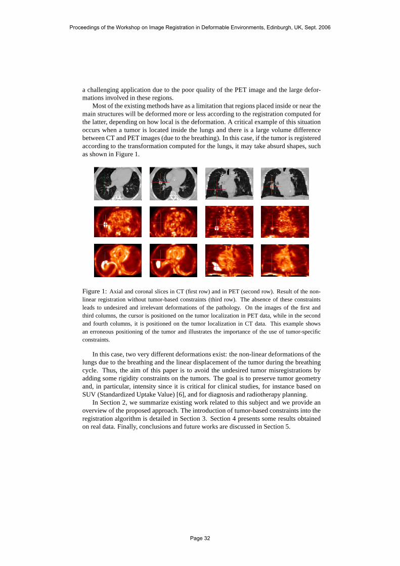
a challenging application due to the poor quality of the PET image and the large defor-mations involved in these regions.

Most of the existing methods have as a limitation that regions placed inside or near themain structures will be deformed more or less according to the registration computed forthe latter, depending on how local is the deformation. A critical example of this situationoccurs when a tumor is located inside the lungs and there is a large volume differencebetween CT and PET images (due to the breathing). In this case, if the tumor is registeredaccording to the transformation computed for the lungs, it may take absurd shapes, suchas shown in Figure 1.

Figure 1:Axial and coronal slices in CT (first row) and in PET (second row). Result of the non-linear registration without tumor-based constraints (third row). The absence of these constraintsleads to undesired and irrelevant deformations of the pathology. On the images of the first andthird columns, the cursor is positioned on the tumor localization in PET data, while in the secondand fourth columns, it is positioned on the tumor localization in CT data. This example showsan erroneous positioning of the tumor and illustrates the importance of the use of tumor-specificconstraints.

In this case, two very different deformations exist: the non-linear deformations of thelungs due to the breathing and the linear displacement of thetumor during the breathingcycle. Thus, the aim of this paper is to avoid the undesired tumor misregistrations byadding some rigidity constraints on the tumors. The goal is to preserve tumor geometryand, in particular, intensity since it is critical for clinical studies, for instance based onSUV (Standardized Uptake Value) [6], and for diagnosis and radiotherapy planning.

In Section 2, we summarize existing work related to this subject and we provide anoverview of the proposed approach. The introduction of tumor-based constraints into theregistration algorithm is detailed in Section 3. Section 4 presents some results obtainedon real data. Finally, conclusions and future works are discussed in Section 5.


Page 32

2 Related Work and Overview of the ProposedApproach

Some approaches have already been developed for registration of multimodality images inpathological cases (pulmonary nodules, cancer), such as in[2]. However these approachescompute a rigid (or affine) registration for all the structures and they do not take intoaccount the local nature of the deformations.

Tanner et al. [15] have developed a method of non-rigid registration based on B-splineFree-Form Deformations (FFD) as in [3]. Their algorithm is applied on MR breast im-ages and it guarantees volume and shape preservation in the rigid regions defined by thelesions. However, the region of the rigid transformation islarger than the lesions. Anotherapproach that uses B-spline FFD is the one by Rohlfing and Maurer [12]. They have useda grid refinement and added some incompressibility constraints (using the properties ofthe Jacobian) which only guarantee the preservation of the volume of the structures butnot their shape. Loeckx et al. [10] have added a local rigidity constraint in order to guar-antee shape preservation and they have obtained very promising results. Nevertheless,this algorithm does not enforce the considered structures to be totally rigid, therefore theyactually might be slightly deformed.

The recent work of Hachama et al. [7] uses a Bayesian framework in order to charac-terize the pathologies as outliers of a probabilistic distribution. Their method is appliedto mammogram registration and proved to be robust. An implicit assumption is that greylevels in both images are similar, thus making the method appropriate for mono-modalityimages. This assumption should be relaxed to extend the method to multimodality images.

A different approach, that we consider closer to physical reality of human body, isbased on the combination of rigid and non-rigid deformations, as suggested by Little etal. [9] and Huesman et al. [8]. These methods are based on the use of point interpolationtechniques, together with a weighting of the deformation according to a distance function.Castellanos et al. [4] developed a slightly different methodology, in which local non-rigidwarpings are used to guarantee the continuity of the transformation.

The advantage of these approaches is that they take into account rigid structures andthe deformations applied to the image are continuous and smooth. The method we pro-pose is inspired by these ones and adapted to develop a registration algorithm for thethoracic region in the presence of pathologies. In order to illustrate our algorithm, wehave applied it on medical data. These data consist of 3D CT and PET images of patho-logical cases, exhibiting tumors in the lungs. We assume that the tumor is rigid and thusa linear transformation is sufficient to cope with its movements between CT and PETimages. This hypothesis is relevant and in accordance with the clinicians’ point of view,since tumors are often a compact mass of pathological tissue. In order to guarantee agood registration of both normal and pathological structures, the first step consists of asegmentation of all structures which are visible in both modalities. Then we define twogroups of landmarks in both images, which correspond to homologous points, and willguide the deformation of the PET image towards the CT image. The positions of thelandmarks are therefore adapted to anatomical shapes. Thisis an important feature andone of the originalities of our method. The deformation at each point is computed usingan interpolation procedure based on the landmarks, on the specific type of deformationof each landmark depending on the structure it belongs to, and weighted by a distancefunction, which guarantees that the transformation will becontinuous.


Page 33

Thus, the proposed approach has two main advantages:

1. As the transformation near the tumor is reduced by using the distance weight, evenif we have some small errors in the tumor segmentation (oftenquite challenging,mainly in CT), we will obtain a consistent and robust transformation.

2. In the considered application, one important fact is thatthe objects to register arenot the same in the two images. For instance, the volume of the“anatomical” tumorin CT is not necessarily the same as the volume of the “functional” tumor in PETbecause the two modalities highlight different characteristics of the objects. Theregistration of these two views of the tumor must preserve these local differences,which can be very useful because we could discover a part of the anatomy thatis touched by the pathology and could not be seen in the CT image. This alsoadvocates in favor of a rigid local registration.

3 Combining Rigid and Non-linear Deformations

Based on a segmentation of the objects visible in both images, pairs of homologous pointsare defined. They constitute landmarks guiding the registration. We assume that globallya non-linear transformation has to be found, while for some objectsO1, . . . ,On0 (tumorsin our application) specific constraints have to be incorporated. For instance, these objectsmay undergo only a rigid transformation between both images. The global transformationis then interpolated over the whole image. We introduce the rigid structures constraints sothat the non-rigid transformation is gradually weighted down in the proximity of objectsO1, . . . ,On0.

Point-Based Displacement InterpolationThe first step in a point-based interpolation algorithm concerns the selection of the

landmarks guiding the transformation. Homologous structures in both images are thenregistered based on landmarks defined on their surface. The resulting deformation will beexact at these landmarks and smooth elsewhere, which is achieved by interpolation.

Let us denote byt i then landmarks in the source image that we want to transform tonew sitesui (the homologous landmarks) in the target image.

The deformation at each pointt in the image is defined as:

f(t) = L (t)+n

∑j=1

BTj σ(t, t j) (1)

under the constraints∀i, ui = f(t i). (2)

The first term,L (t), represents the linear transformation of every pointt in the sourceimage. Whenn0 rigid objects (O1,O2, . . . ,On0) are present, the linear term is a weightedsum of each object’s linear transformation. The weightswi(t) are dependent on a measureof distanced(t,Oi) from the pointt to the objectOi as described in [9]:

wi(t) =

1 if t ∈ Oi

0 if t ∈ O j , j = 1, . . . ,n0, j 6= iqi(t)

∑n0j=1 q j (t)

otherwisewhere qi(t) =

1d(t,Oi)µ (3)


Page 34

andµ = 1.5 (for the work illustrated in this paper).Therefore, for any pointt we define our linear transformation as:

L (t) =n0

∑i=1

wi(t)Li (4)

whereLi , i = 1, . . . ,n0 are the linear transformations of the rigid objects. The closert isto the objectOi , the more similar its linear transformation will be toLi .

The second term represents the non-linear transformation which is, for a pointt, thesum ofn terms, one for each landmark. Each term is the product of the coefficients of amatrixB (that will be computed in order to satisfy the constraints onthe landmarks) witha functionσ(t, t j), depending on the (normalized) distance betweent andt j :

σ(t, t j) = |t − t j|. (5)

This form has favorable properties for image registration [17]. However, different func-tions could be used, as the one described in [9].

With the constraints given by Equation 2, we can calculate the coefficientsB of thenon-linear term by expressing Equation 1 fort = t i . The transformation can then bedefined in a matricial way:

ΣB+L = U (6)

whereU is the matrix of the landmarksui in the target image (the constraints),Σi j =σ(t i , t j) (given by Equation 5),B is the matrix of the coefficients of the non-linear termand L represents the application of the linear transformations to the landmarks in thesource image,t i .

From Equation 6, the matrixB is obtained as:B = Σ−1(U −L). Once the coefficientsof B are found, we can calculate the general interpolation solution for every point inR

3

as shown in Equation 1.

Introducing Rigid StructuresIn this section, we show how to introduce the constraints imposed by the rigid structures

in the images.To add the influence of the rigid structuresO1, . . . ,On0, we have redefined the function

σ(t, t j) asσ ′(t, t j) in the following way:

σ ′(t, t j) = d(t,O0)d(t j ,O0)σ(t, t j) (7)

whered(t,O0) is a measure of the distance from pointt to the union of rigid objectsO0 = O1∪O2∪ . . .∪On0. It is equal to zero fort ∈ O0 (inside any of the rigid structures)and takes small values whent is near one of the structures. This measure of the distanceis continuous overR3 and it weights the functionσ(t, t j) (see Equation 5). Thus theimportance of the non-linear deformation is controlled by the distance to the rigid objectsin the following manner:

• d(t,O0) makesσ ′(t, t j) tend towards zero when the point for which we are calcu-lating the transformation is close to one of the rigid objects;

• d(t j ,O0) makesσ ′(t, t j) tend towards zero when the landmarkt j is near one of therigid objects. This means that the landmarks close to the rigid structures hardlycontribute to the non-linear transformation computation.


Page 35

Note that this formalism could be more general by replacingd(t,O0) by any functionof the distance toO0 that characterizes accurately the behavior of the surrounding regions.Further research is necessary to define such a function in thecase of lung tumors. We haveused a linear (normalized) distance function as a first approach.

Finally, Equation 6 is rewritten by replacingΣ by Σ′, leading to a new matrixB′. Wecan then calculate the general interpolation solution for every point inR

3 as in Equation 1.

Definition of landmarks and matchingLandmarks can be defined according to the needs of each specific application. They can

be uniformly distributed over the surface of homologous objects or based on points havingspecific properties (maximum of curvature, points undergoing the largest deformations,etc). In our application, we first define a set of landmarks on the surface of the lungson the CT image, because it has a much better resolution than the PET image. They areapproximately uniformly distributed on the surface. Then,we calculate the correspondingpoints on the surface of the segmented lungs in PET. This is automatically computed byusing the Iterative Closest Point (ICP) algorithm [1] and avoids defining by hand thelandmarks on both images.

4 Results

We present in this section some results that we have obtainedon synthetic, segmentedand real images. The structures and the tumors are segmentedusing the methods in [5]and then, based on pairs of corresponding landmarks in the CTand the PET images,the transformation is computed over the whole image. As mentioned in Section 2, it isreasonable to assume a rigid transformation between the tumors in CT and in PET. Asa first approach, we have used a translation. Each translation Li , i = 1, . . . ,n0 is directlyobtained from the segmentation results.

Synthetic imagesThis first experiment on synthetic images aims at checking that the rigid structures are

transformed rigidly, that the landmarks are correctly translated too and, finally, that thetransformation elsewhere is consistent and smooth.

Figure 2:Result on synthetic images: the effect of expanding a frame (in grey in the figure) andtranslating the “tumor” (in white in the figure). The source image (with a grid) is shown on the left,the target image is in the middle and the result of the transformation on the right. The landmarksare located on the internal and external edges of the frame ingrey (on the corners and in the middleof the sides). The total number of landmarks is 16.

As we are taking the PET image as the one to be deformed (sourceimage), we sim-ulate an expansive transformation because the lungs in PET are usually smaller than in


Page 36

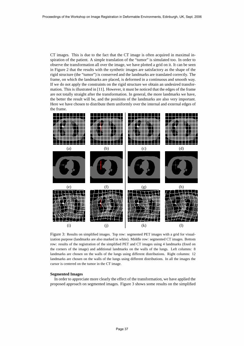
CT images. This is due to the fact that the CT image is often acquired in maximal in-spiration of the patient. A simple translation of the “tumor” is simulated too. In order toobserve the transformation all over the image, we have plotted a grid on it. It can be seenin Figure 2 that the results with the synthetic images are satisfactory as the shape of therigid structure (the “tumor”) is conserved and the landmarks are translated correctly. Theframe, on which the landmarks are placed, is deformed in a continuous and smooth way.If we do not apply the constraints on the rigid structure we obtain an undesired transfor-mation. This is illustrated in [11]. However, it must be noticed that the edges of the frameare not totally straight after the transformation. In general, the more landmarks we have,the better the result will be, and the positions of the landmarks are also very important.Here we have chosen to distribute them uniformly over the internal and external edges ofthe frame.

(a) (b) (c) (d)

(e) (f) (g) (h)

(i) (j) (k) (l)

Figure 3:Results on simplified images. Top row: segmented PET images with a grid for visual-ization purpose (landmarks are also marked in white). Middle row: segmented CT images. Bottomrow: results of the registration of the simplified PET and CT images using 4 landmarks (fixed onthe corners of the image) and additional landmarks on the walls of the lungs. Left columns: 8landmarks are chosen on the walls of the lungs using different distributions. Right columns: 12landmarks are chosen on the walls of the lungs using different distributions. In all the images thecursor is centered on the tumor in the CT image.

Segmented ImagesIn order to appreciate more clearly the effect of the transformation, we have applied the

proposed approach on segmented images. Figure 3 shows some results on the simplified


Page 37

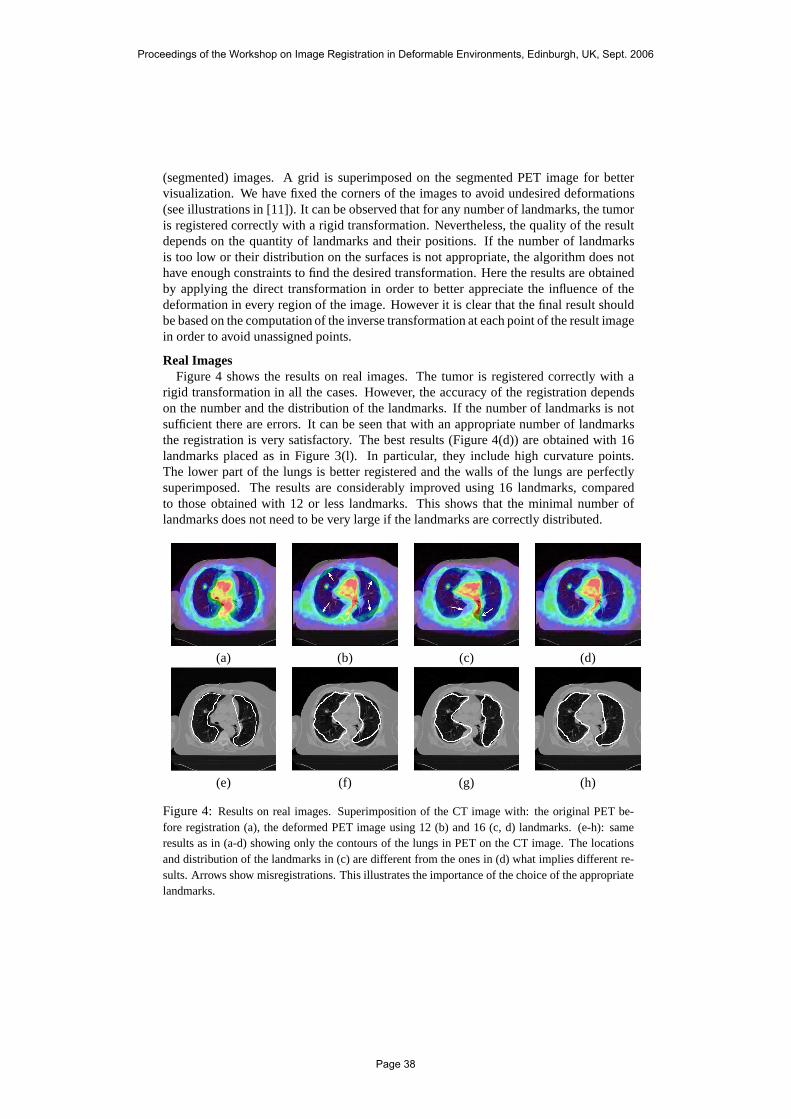
(segmented) images. A grid is superimposed on the segmentedPET image for bettervisualization. We have fixed the corners of the images to avoid undesired deformations(see illustrations in [11]). It can be observed that for any number of landmarks, the tumoris registered correctly with a rigid transformation. Nevertheless, the quality of the resultdepends on the quantity of landmarks and their positions. Ifthe number of landmarksis too low or their distribution on the surfaces is not appropriate, the algorithm does nothave enough constraints to find the desired transformation.Here the results are obtainedby applying the direct transformation in order to better appreciate the influence of thedeformation in every region of the image. However it is clearthat the final result shouldbe based on the computation of the inverse transformation ateach point of the result imagein order to avoid unassigned points.

Real ImagesFigure 4 shows the results on real images. The tumor is registered correctly with a

rigid transformation in all the cases. However, the accuracy of the registration dependson the number and the distribution of the landmarks. If the number of landmarks is notsufficient there are errors. It can be seen that with an appropriate number of landmarksthe registration is very satisfactory. The best results (Figure 4(d)) are obtained with 16landmarks placed as in Figure 3(l). In particular, they include high curvature points.The lower part of the lungs is better registered and the wallsof the lungs are perfectlysuperimposed. The results are considerably improved using16 landmarks, comparedto those obtained with 12 or less landmarks. This shows that the minimal number oflandmarks does not need to be very large if the landmarks are correctly distributed.

(a) (b) (c) (d)

(e) (f) (g) (h)

Figure 4: Results on real images. Superimposition of the CT image with: the original PET be-fore registration (a), the deformed PET image using 12 (b) and 16 (c, d) landmarks. (e-h): sameresults as in (a-d) showing only the contours of the lungs in PET on the CT image. The locationsand distribution of the landmarks in (c) are different from the ones in (d) what implies different re-sults. Arrows show misregistrations. This illustrates theimportance of the choice of the appropriatelandmarks.


Page 38

5 Conclusion and Future Work

We have developed a non-linear registration method incorporating constraints on defor-mations of specified objects. It has been shown to be adapted to images which containrigid structures. The method consists in computing a deformation guided by a group oflandmarks and with rigidity constraints. This method has been illustrated on the exam-ple of CT/PET registration, in pathological cases where most tissues undergo non-lineartransformations due to breathing while tumors remain rigid. In this application, results arevery satisfactory and our algorithm avoids undesired tumormisregistrations and preservestumor geometry and intensity.

One of the originalities of our approach, in particular compared to the method in [9],is that the positions of the landmarks are adapted to the shapes of the structures in theimages. In addition to this, with our algorithm, the landmarks are only defined manuallyin one of the images (the CT) and automatically in the second one (the PET) by meansof the ICP algorithm. In the illustrated application, as thetransformation near the tumoris reduced by a weight depending on a distance measure, even if the tumor segmentationis not perfect, the registration remains consistent and robust. Moreover, the tumor in CTand PET has not necessarily the same size and shape, therefore the registration of thesetwo modalities is very useful because all the information ofthe PET image is preserved.This is very important in order to know the true extension of the pathology for diagnosisand for the treatment of the tumor with radiotherapy, for example.

The choice of the landmarks in the CT image is done manually for the moment. How-ever, future work aims at developing an automatic method fordefining the landmarkshomogeneously distributed all over the surface and on the regions of maximum curvature.A quantitative measure of the alignment between the images will be used in order to findthe best distribution of the landmarks that minimizes this similarity measure.

It is also necessary to carry out a detailed study of the rigidity properties of the tis-sues surrounding a pathology. Replacing the distance by another function would then bestraightforward using our formulation.

Although validation is a common difficulty in registration [13], we plan an evaluationphase in collaboration with clinicians, as well as comparison with other methods.

AcknowledgementsThe authors would like to thank Liege, Lille, Louisville and Val de Grace Hospitals

for the images and helpful discussions and the members of Segami Corporation for theircontribution to this project. This work was partially supported by the French Ministry forResearch.

References[1] P. J. Besl and N. D. McKay. A Method for Registration of 3-DShapes.IEEE Transactions on

Pattern Analysis and Machine Intelligence, 14(2):239–256, February 1992.

[2] T. Blaffert and R. Wiemker. Comparison of Different Follow-Up Lung Registration Methodswith and without Segmentation. InProceedings of SPIE Medical Imaging 2004, volume 5370,pages 1701–1708, San Diego, California, USA, February 2004.


Page 39

[3] O. Camara-Rey.Non-Linear Registration of Thoracic and Abdominal CT and PET Images:Methodology Study and Application in Clinical Routine. PhD thesis, ENST 2003 E 043, EcoleNationale Superieure des Telecommunications (ENST), Paris, France, December 2003.

[4] N. P. Castellanos, P. L. D. Angel, and V. Medina. NonrigidMedical Image RegistrationTechnique as a Composition of Local Warpings.Pattern Recognition, 37:2141–2154, 2004.

[5] G. Delso. Registro Elastico de Imagenes Medicas Multimodales. Aplicacion en Oncologıa.PhD thesis, Centre de Recerca en Enginyeria Biomedica, Universitat Politecnica de Catalunya,Barcelona, Spain, October 2003.

[6] J. Feuardent, M. Soret, O. de Dreuille, H. Foehrenbach, and I. Buvat. Reliability of SUVEstimates in FDG PET as a Function of Acquisition and Processing Protocols. InProceedingsof the IEEE Nuclear Science Symposium Conference Record, volume 4, pages 2877–2881,October 2003.

[7] M. Hachama, F. Richard, and A. Desolneux. A Mammogram Registration Technique DealingWith Outliers. InProceedings of the IEEE International Symposium on Biomedical Imaging(ISBI’06), Arlington, Virginia, USA, April 2006.

[8] R. H. Huesman, G. J. Klein, J. A. Kimdon, C. Kuo, and S. Majumdar. Deformable Registra-tion of Multimodal Data Including Rigid Structures.IEEE Transactions on Nuclear Science,50(3):4S–14S, June 2003.

[9] J. A. Little, D. L. G. Hill, and D. J. Hawkes. DeformationsIncorporating Rigid Structures.Computer Vision and Image Understanding, 66(2):223–232, May 1997.

[10] D. Loeckx, F. Maes, D. Vandermeulen, and P. Suetens. Nonrigid Image Registration UsingFree-Form Deformations with Local Rigidity Constraint. InProceedings of MICCAI 2004,volume LNCS 3216, pages 639–646, Rennes - St-Malo, France, September 2004.

[11] A. Moreno, G. Delso, O. Camara, and I. Bloch. CT and PET Registration Using DeformationsIncorporating Tumor-Based Constraints. InProceedings of the 10th Iberoamerican Congresson Pattern Recognition (XCIARP), volume LNCS 3773, pages 1–12, La Habana, Cuba, nov2005.

[12] T. Rohlfing and C. R. Maurer. Intensity-Based Non-RigidRegistration Using Adaptive Mul-tilevel Free-Form Deformation with an Incompressibility Constraint. InProceedings of MIC-CAI 2001, volume LNCS 2208, pages 111–119, Utrecht, The Netherlands, October 2001.

[13] J. A. Schnabel, C. Tanner, A. D. Castellano-Smith, A. Degenhard, M. O. Leach, D. R. Hose,D. L. G. Hill, and D. J. Hawkes. Validation of Nonrigid Image Registration Using Finite-Element Methods: Application to Breast MR Images.IEEE Transactions on Medical Imaging,22(2):238–247, February 2003.

[14] R. Shekhar, V. Walimbe, S. Raja, V. Zagrodsky, M. Kanvinde, G. Wu, and B. Bybel. Au-tomated 3-Dimensional Elastic Registration of Whole-BodyPET and CT from Separate orCombined Scanners.The Journal of Nuclear Medicine, 46(9):1488–1496, September 2005.

[15] C. Tanner, J. A. Schnabel, D. Chung, M. J. Clarkson, D. Rueckert, D. L. G. Hill, and D. J.Hawkes. Volume and Shape Preservation of Enhancing LesionsWhen Applying Non-rigidRegistration to a Time Series of Contrast Enhancing MR Breast Images. InProceedings ofMICCAI 2000, volume LNCS 1935, pages 327–337, Pittsburgh, USA, 2000.

[16] H. N. Wagner. PET and PET/CT: Progress, Rewards, and Challenges.The Journal of NuclearMedicine, 44(7):10N–14N, July 2003.

[17] R. Wiemker, K. Rohr, L. Binder, R. Sprengel, and H. S. Stiehl. Application of Elastic Regis-tration to Imagery from Airbone Scanners. InXVIII Congress of the International Society forPhotogrammetry and Remote Sensing (ISPRS’96), volume XXXI-B4, pages 949–954, Vienna,Austria, 1996.


Page 40

Evaluation of a Rigidity Penalty Term forNonrigid Registration

Marius Staring, Stefan Klein and Josien P.W. Pluim

Image Sciences Institute, University Medical Center Utrecht,P.O. Box 85500, 3508 GA, Room Q0S.459, Utrecht, The Netherlands,

marius,stefan,[email protected]

Abstract

Nonrigid registration of medical images usually does not model properties ofdifferent tissue types. This results for example in nonrigid deformations ofstructures that are rigid. In this work we address this problem by employ-ing a local rigidity penalty term. We illustrate this approach on a 2D syn-thetic image, and evaluate it on clinical 2D DSA image sequences, and on3D CT follow-up data of the thorax of patients suffering from lung tumours.The results show that the rigidity penalty term does indeed penalise nonrigiddeformations of rigid structures, whereas the standard nonrigid registrationalgorithm compresses those.

1 Introduction

Nonrigid registration of patient data is an important technique in the field of medicalimaging. One of the remaining problems of nonrigid registration algorithms is that usuallyeverything in the images is treated as nonrigid tissue, even objects that are clearly rigid,or objects for which it is desired to keep them rigid. Examples of the first are bonesand surgical instruments. Examples of the second include structures that contain contrastmaterial, visible in one image, but not in the other. Standard intensity based nonrigidregistration algorithms will typically give undesired compression of these structures [10,15]. It is necessary to prevent nonrigid behaviour of these local structures, and keep themrigid instead.

In the literature several methods have been described to constrain deformations. Theemployment of a regularisation or penalty term is a well-known strategy. Examples ofsuch terms are the bending energy of a thin plate [12], the linear elasticity constraint[1, 2] and the incompressibility constraint [10]. Particular methods to enforce rigidityon structures have also been proposed. Tanner et al. [15] propose to couple the controlpoints of a B-spline deformation. Another approach is taken by Little et al. [6], who usemodified basis functions describing the deformation, constraining the nonlinear part ofthe deformation at rigid locations by multiplication with a weight function.

Recently, some approaches similar to our own were published [7, 11], in which rigid-ity is enforced by penalising deviation of the Jacobian from being orthonormal. In thispaper we propose a penalty term that is capable of penalising locally nonrigid transforma-tions, which we call a rigidity penalty term. It is based on three criteria a transformation


Page 41

must meet in order to be locally rigid: linearity of the transformation, and orthonormalityand properness of the Jacobian of the transformation. First results of the method werepublished previously [14].

In the following section we describe the rigidity penalty term. Standard nonrigidregistration is compared against registration using the rigidity penalty term in Section 3.We end with a discussion in Section 4.

2 Method

Registration of a moving image M(xxx) : ΩM ⊂Rd →R to a fixed image F(xxx) : ΩF ⊂R

d →R, both of dimension d, consists of finding a deformation uuu(xxx) that makes M(xxx + uuu(xxx))spatially aligned to F(xxx). The quality of alignment is defined by a similarity or distancemeasure D , such as the sum of squared differences (SSD), the correlation ratio, or themutual information (MI) measure.

Because this problem is ill-posed, a regularisation term or smoother S is introducedand the registration problem is formulated as an optimisation problem in which a costfunction J is minimised w.r.t. uuu, with:

J [F,M;uuu] = D [F,M;uuu]+αS [uuu], (1)

where α weighs similarity against smoothness. Note that at the minimum the derivativesof the similarity measure and the regularisation term are not necessarily zero. Merely, abalance is found between the two, which is influenced by the parameter α . Therefore, thepenalty term can not be considered a hard constraint, but it is sometimes referred to as asoft constraint.

In [14] we propose a penalty term S rigid[u] that penalises nonrigid deformations ofrigid objects, which we call the rigidity penalty term. This penalty term can be weightedlocally, so that some parts of the image are restricted to rigid movement, while other partsare penalised partially or are allowed to deform freely.

2.1 Registration Algorithm

We employ a registration framework largely based on the papers of Rueckert et al. [12]and Mattes et al. [8]. The similarity measure is the mutual information measure usingan implementation by Thevenaz and Unser [16]. The deformation field is parameterisedby cubic B-splines. A multiresolution approach is taken to avoid local minima, using aGaussian pyramid with a subsampling factor of two in each dimension. We also employa multiresolution approach of the deformation grid: when the image resolution in thepyramid is doubled, the B-spline control point spacing is halved. For the optimisationof the cost function J , we employ a stochastic gradient descent optimiser, using only asmall, randomly chosen portion of the total number of pixels for calculating the derivativeof J with respect to the B-spline parameters [5].

2.2 Construction of the Rigidity Penalty Term

The rigidity penalty term S rigid[u] is constructed by penalising deviation from three con-ditions. For a deformation field uuu to be rigid, it must hold that uuu(xxx)+ xxx = Rxxx+ ttt, with R


Page 42

and ttt a rotation matrix and a translation vector, respectively. Note that the rotation matrixR is the Jacobian of the transformation uuu(xxx)+ xxx. The three conditions are (given in 2Dfor readability):

linearity of uuu(xxx), stating that the second order derivatives are zero:

LCki j(xxx) =∂ 2uk(xxx)∂xi∂x j

= 0, (2)

for all k, i, j = 1,2, not counting duplicates.

orthonormality of R, which can be expressed in terms of derivatives of uuu(xxx):

OCi j(xxx) =2

∑k=1

(

∂uk(xxx)∂xi

+δki

)(

∂uk(xxx)∂x j

+δk j

)

−δi j = 0, (3)

for all i, j = 1,2, again not counting duplicates.

properness of R: PC(xxx) = det(R)− 1 = 0, which can again be expressed in terms ofderivatives of uuu(xxx). Note that this condition basically amounts to an incompress-ibility constraint, see also [10].

We define the rigidity penalty term S rigid[uuu] to be the sum of these conditions squared.In order to distinguish between rigid and nonrigid tissue, the penalty term is weighted bya so-called rigidity coefficient c(xxx) ∈ [0,1] of the tissue type at position xxx. The completeexpression reads:

S rigid[uuu] ∑xxx∈ΩF

c(xxx)

∑k,i, j

[

LCki j(xxx)]2

+∑i, j

[OCi j(xxx)]2 +[PC(xxx)]2

. (4)

The rigidity coefficient c(xxx) is equal to zero for pixels xxx in completely nonrigid tissue,thereby not penalising deformations at those locations. For completely rigid tissue c(xxx)is set to one. For other tissue types a value of c(xxx) is chosen between zero and one.The rigidity coefficient image can be constructed by performing a manual or automaticsegmentation of structures of interest, after which rigidity coefficients can be assigned.Depending on the application, different methods to create the rigidity coefficient imagecan be considered. For the case of CT images the Hounsfield unit might be used, rescaledto the range [0,1], since more rigid tissue usually has a higher attenuation value.

In [14] we argue the validity of this rigidity penalty term by showing that S rigid[uuu] = 0if and only if the deformation field uuu(xxx) is locally rigid. The linearity term might bedropped, since it can be shown that orthonormality implies linearity. However, it mightaid the penalty term by guiding the optimisation path. The proposed constraint is notdependent on the B-spline parameterisation of the deformation field. However, from acomputational point of view, we can benefit from this parameterisation by evaluating therigidity penalty term only over the control points. For details we refer to [14].

3 Experiments and Results

Standard nonrigid registration using only the similarity term, as described in Section 2.1,is compared with nonrigid registration using the rigidity penalty term. The two methods


Page 43

(a) (b) (c)

Figure 1: Comparison of registration with and without S rigid[uuu] for a 2D synthetic ex-ample. The white square is to be kept rigid. (a) fixed image (lower) and moving image(upper), (b) resulting deformation field of standard registration, and (c) resulting defor-mation field including the rigidity constraint.

are illustrated on synthetic images. They are compared on clinical data, viz. 3D CTfollow-up data of the thorax containing lung tumours, and on 2D DSA image data ofdifferent parts of the body. The computation time for registration with the rigidity penaltyterm increases about 50% in 2D and about 80% in 3D with a B-spline grid spacing ofeight voxels.

All experiments were performed with software (www.isi.uu.nl/Elastix/) devel-oped by the authors. This registration package is largely based on the Insight Segmenta-tion and Registration Toolkit [4].

3.1 2D Synthetic Example

Rotation of a rigid object is illustrated with the square in Figure 1, where the backgroundrepresents nonrigid tissue and the square a rigid object. The rigidity coefficient c(xxx) is setto 1.0 on the square and 0.0 elsewhere.

Both algorithms give near perfect registration results for the matching of the squaresin Figure 1. However, the underlying deformation field is highly nonlinear if no rigiditypenalty term is used. By including the penalty term the deformation field is almost per-fectly rigid at the rigid part. This is also reflected in the rigidity constraint S rigid[uuu], whichhas a value of 2.21×102 for standard nonrigid registration and a value of 1.28×10−3 forregistration using the rigidity constraint. The rigidity constraint is not perfectly zero, be-cause some B-spline control points outside the square, but influencing the points withinthe square, are not set to be rigid.

3.2 3D CT Follow-up

In order to compare 3D CT follow-up data by visual inspection of the difference im-age, the data sets must be registered nonrigidly. We have five CT follow-up data sets ofthe thorax available, of patients suffering from lung tumours, collected at the Radiologydepartment of the University Medical Centre Utrecht. The images are acquired under


Page 44

(a) (b) (c)

(d) (e) (f)

Figure 2: Comparison of both nonrigid registration methods for a slice taken from 3DCT thorax images. The tumours, located within the box (see (d)), have to be kept rigidfor diagnostic reasons. (a) and (d): CT slice at time t0 (the fixed image) and time t1(the moving image), respectively, (b) and (c): difference of the result of similarity onlynonrigid registration with the fixed image, and a part of the resulting deformation field,respectively, (e) and (f): the same for nonrigid registration using S rigid[uuu].

breath-hold with a Philips 16 slice spiral CT scanner (Mx8000 IDT 16). The data areof size 512× 512 by 400 - 550 slices, have voxel sizes of around 0.7× 0.7× 0.7 mm,and are resized by a factor of 2 in each dimension before registration. The five data setscontain 36 tumours in total, with an average volume of 2.5 ml for the first scan and 5.1 mlat the second. The CT image taken at time t0 is set to be the fixed image, the follow-upCT image (time t1) the moving image. For visual inspection of the tumour growth fromthe difference image, the tumours must not deform nonrigidly, but only in a rigid fash-ion. This way tumour growth can be seen from the difference image, in relation with theanatomy shown in the CT image. For an example of the difference image in these cases,see Figure 2(b) and 2(e). Tumour growth is effectively concealed in the similarity onlybased registration.

To get a coarse alignment between fixed and moving image a rigid registration is per-formed first. Then the nonrigid registration is performed, using a B-spline grid spacing of8 voxels, 4 resolutions, 300 iterations per resolution, and 5000 voxel samples to calculate(the derivative of) the mutual information. For the nonrigid registration with the rigid-ity penalty term, the tumour regions are defined by a crude manual delineation, setting


Page 45

Table 1: Average lung overlap.

before registration rigid similarity only with S rigid[uuu]

0.64 ± 0.22 0.91 ± 0.06 0.98 ± 0.01 0.97 ± 0.02

c(xxx) = 1.0 in the tumour regions and 0.0 elsewhere.Accuracy of the registration is measured by calculating the lung overlap of the regis-

tered image with the fixed one. For this purpose automatic lung segmentations are madewith an algorithm based on the method by Hu et al. [3,13]. The overlap measure is definedas

overlap 2 · |L1 ∩L2||L1|+ |L2| , (5)

where Li is the set of all voxels from the lung, and where |Li| is the size of set Li. Fromthe results reported in Table 1, we see that both registrations lead to good lung overlap.Employing a rigidity penalty term, constrains the deformation, leading to a slightly lessaccurate lung overlap. Because of the (compact) support of the B-splines, a boundaryaround the tumour is influenced by the control points within the tumour. The extent ofthis boundary can be controlled with the B-spline grid spacing.

Manual segmentations of the tumours are used to evaluate their rigidity. Tumour vol-ume measurements are performed to see if the registration is at least volume preserving.In order to compare tumours volumes with different sizes we can not use the arithmeticmean, because large tumours influence the arithmetic mean disproportionally. Therefore,volume growth ratios are calculated, where every tumour volume is divided by its volumeat t1. For growth ratios it is better to use the geometric mean and the geometric standarddeviation, which are defined as:

µg = n

√

n

∏i=1

ri , σg = exp

(√

1n

n

∑i=1

(lnri − ln µg)2

)

, (6)

where ri denotes the growth ratio of tumour i. We report the geometric mean growthratios and standard deviations in Table 2. It can be appreciated that volume is much betterpreserved when applying the rigidity penalty term, compared to similarity only basedregistration. Part of the residual volume difference can be explained by interpolationartifacts due to resampling, as can be seen from the results for rigid registration. Fromthe deformation field, see Figure 2(f) (compare with 2(c)) is can also be appreciated thatnonrigid registration using the rigidity penalty term preserves rigidity locally.

3.3 Digital Subtraction Angiography

Evaluation is also performed on 2D clinical digital X-ray angiography image data, ac-quired with an Integris V3000 C-arm imaging system (Philips). Digital Subtraction An-giography (DSA) imaging often suffers from motion artifacts, due to motion of or withinthe patient, see Figure 3(a) - 3(c). Nonrigid registration is needed to compensate for this.We have 26 image sequences available of twelve different patients, each containing about10 images. Images are mostly of size 512×512 and are taken of different locations in the


Page 46

Table 2: Geometric mean tumour volume ratios. Geometric means are calculated for fourgrowth groups and for all growth ratios. The second group for example is the group oftumours that corresponds to a volume ratio t1/t0 between 1 and 3/2.

group t1/t0 t0 rigid similarity only with S rigid[uuu]

(0,1] 1.18 ×/ 1.08 0.99 ×/ 1.02 1.00 ×/ 1.03 0.96 ×/ 1.06(

1, 32

]

0.84 ×/ 1.05 0.96 ×/ 1.04 0.97 ×/ 1.05 1.03 ×/ 1.03(

32 ,3

]

0.48 ×/ 1.10 1.00 ×/ 1.02 0.79 ×/ 1.07 1.00 ×/ 1.02

(3,∞) 0.23 ×/ 1.13 1.02 ×/ 1.03 0.69 ×/ 1.12 0.99 ×/ 1.02

all 0.52 ×/ 1.29 0.99 ×/ 1.03 0.83 ×/ 1.10 1.00 ×/ 1.03

body, such as the abdomen, the brain, neck and lungs. Because it takes time for the con-trast bolus to travel through the vasculature, different parts of the vasculature are visibleat different times. If the whole vasculature is to be extracted, all images have to be regis-tered to some baseline image. For this, we choose the first image in each sequence, whichis taken before arrival of the contrast bolus, to be the fixed image. For this experimentwe register only one of the other images to the fixed image: the image showing most ofthe vasculature is chosen as the moving image. The nonrigid registration of DSA imagescan lead to undesired compression of the vasculature, as reported in [9] for CT-DSA. Al-though the vessels are not intrinsically rigid, they are to be kept rigid, since there existsno information to do otherwise: vessels are visible in one image and not in the other.

We applied a rigid registration first for coarse alignment. For the nonrigid registrationwe use a B-spline grid spacing of 16 pixels, 2 resolutions, 600 and 300 iterations perresolution, and 5000 samples for calculating (the derivative of) the MI. A crude manualsegmentation of the vessels is used for defining c(xxx).

To measure the success of the nonrigid registration, the Mean Square Difference(MSD) of the background B is calculated. The MSD is defined as:

MSD =1

|B| ∑xxx∈B

(

F(xxx)−M(xxx+uuu(xxx))

)2

. (7)

Results are shown in the top row of Table 3, showing improvement of this measure fornonrigid registration. Compare also Figure 3(d) with Figure 3(e) and 3(e). As a measureof rigidity, vessel diameter measurements are carried out to quantify vessel compression.In every one of the 26 images six diameter measurements are carried out. The geometricmean of the vessel diameter ratios are reported in the bottom row of Table 3. Withoutemploying the rigidity penalty term the vessels are severely compressed, which is avoidedwith the use of S rigid[uuu]. The shape of the deformation fields confirms this, see Figure3(g) and 3(g).

4 Conclusions and Discussion

We have proposed a method to perform nonrigid registration, while keeping user-definedlocal structures rigid. This is achieved by adding a rigidity penalty term to the registration


Page 47

(a) (b) (c)

(d) (e) (f)

(g) (h)

Figure 3: Comparison of different registration algorithms for 2D DSA images. The ves-sels are to be kept rigid, while motion artifacts are to be reduced by the registration. (a)DSA baseline image: the fixed image, (b) DSA image after injection of the contrast bolus:the moving image, (c) - (f) are difference images with the fixed image, (c) with the mov-ing image, (d) with the result of rigid registration, (e) with the result of similarity onlynonrigid registration, (f) with the result of nonrigid registration using the rigidity penaltyterm. The bottom row depicts parts of the resulting deformation field of similarity only(g), and using the rigidity penalty term (h). The black box in Figure (e) and (f) denotesthe part of the deformation field that is depicted.

framework (1). The method is illustrated on a synthetic 2D example and evaluated on 2Dand 3D clinical data.


Page 48

Table 3: Results for DSA. Arithmetic means for the MSD and geometric means for thevessel diameter ratios compared with t1.

no registration rigid similarity only with S rigid[uuu]

MSD 231 ± 205 215 ± 181 163 ± 105 171 ± 128

diameter 1.00 ×/ 1.00 1.00 ×/ 1.00 0.85 ×/ 1.07 0.99 ×/ 1.01

From the results we can see that the rigidity penalty term indeed penalises nonrigiddeformations, but complete rigidity is sometimes not achieved. Some reasons are thefollowing. 1) The rigidity penalty term is not a hard constraint, it is merely a tradeoffbetween similarity and penalty. 2) For the case of modelling the deformation field withcubic B-splines, the control points outside a rigid structure influence the inside. Therefore,if complete rigidity is wanted, the two adjacent control points outside the structure mustalso be kept rigid, for example by performing a dilation on the rigidity coefficient imagec(xxx). Of course the inverse is also true: the rigid part influencing the nonrigid part, therebyrestricting the deformation at the boundaries of the rigid structure. The extent of thisboundary is controlled by the B-spline control point spacing.

The linearity condition (2) might not be necessary, since it can be shown that orthonor-mality of the Jacobian of uuu implies linearity of uuu. However, it might guide the optimiserin reaching rigidity; this is interesting future work.

Acknowledgments

This research was funded by the Netherlands Organisation for Scientific Research (NWO).This work also benefited from the use of the Insight Segmentation and Registration Toolkit(ITK). We gratefully acknowledge Oskar Skrinjar for a fruitful discussion about the lin-earity condition of the rigidity penalty term.

References

[1] G. E. Christensen and H. J. Johnson. Consistent image registration. IEEE Transac-tions on Medical Imaging, 20(7):568 – 582, 2001.

[2] B. Fischer and J. Modersitzki. A unified approach to fast image registration and anew curvature based registration technique. Linear Algebra and its Applications,380:107 – 124, 2004.

[3] S. Hu, E. A. Hoffman, and J. M. Reinhardt. Automatic lung segmentation for accu-rate quantitation of volumetric X-Ray CT images. IEEE Transactions on MedicalImaging, 20(6):490 – 498, 2001.

[4] Luis Ibanez, Will Schroeder, Lydia Ng, and Josh Cates. The ITK Software Guide.Kitware, Inc. ISBN 1-930934-15-7, second edition, 2005.

[5] S. Klein, M. Staring, and J. P. W. Pluim. Comparison of gradient approximationtechniques for optimisation of mutual information in nonrigid registration. In SPIE


Page 49

Medical Imaging: Image Processing, volume 5747, pages 192 – 203. SPIE Press,2005.

[6] J. A. Little, D. L. G. Hill, and D. J. Hawkes. Deformations incorporating rigidstructures. Computer Vision and Image Understanding, 66(2):223 – 232, 1997.

[7] D. Loeckx, F. Maes, D. Vandermeulen, and P. Suetens. Nonrigid image registrationusing free-form deformations with a local rigidity constraint. In MICCAI, volume3216 of Lecture Notes in Computer Science, pages 639 – 646. Springer Verlag, 2004.

[8] D. Mattes, D. R. Haynor, H. Vesselle, T. K. Lewellen, and W. Eubank. PET-CTimage registration in the chest using free-form deformations. IEEE Transactions onMedical Imaging, 22(1):120 – 128, 2003.

[9] T. Rohlfing and C. R. Maurer Jr. Intensity-based nonrigid registration using adaptivemultilevel free-form deformation with an incompressibility constraint. In MICCAI,volume 2208 of Lecture Notes in Computer Science, pages 111 – 119. SpringerVerlag, 2001.

[10] T. Rohlfing, C. R. Maurer Jr., D. A. Bluemke, and M. A. Jacobs. Volume-preservingnonrigid registration of MR breast images using free-form deformation with an in-compressibility constraint. IEEE Transactions on Medical Imaging, 22(6):730 –741, 2003.

[11] D. Ruan, J. A. Fessler, M. Roberson, J. Balter, and M. Kesler. Nonrigid registra-tion using regularization that accomodates local tissue rigidity. In SPIE MedicalImaging: Image Processing, volume 6144, pages 346 – 354. SPIE Press, 2006.

[12] D. Rueckert, L. I. Sonoda, C. Hayes, D. L. G. Hill, M. O. Leach, and D. J. Hawkes.Nonrigid registration using free-form deformations: Application to breast MR im-ages. IEEE Transactions on Medical Imaging, 18(8):712 – 721, 1999.

[13] I. C. Sluimer, M. Prokop, and B. van Ginneken. Towards automated segmentationof the pathological lung in CT. IEEE Transactions on Medical Imaging, 24(8):1025– 1038, 2005.

[14] M. Staring, S. Klein, and Josien P. W. Pluim. Nonrigid registration using a rigidityconstraint. In SPIE Medical Imaging: Image Processing, volume 6144 of Proceed-ings of SPIE, pages 355 – 364. SPIE Press, 2006.

[15] C. Tanner, J. A. Schnabel, D. Chung, M. J. Clarkson, D. Rueckert, D. L. G. Hill, andD. J. Hawkes. Volume and shape preservation of enhancing lesions when applyingnonrigid registration to a time series of contrast enhancing MR breast images. InMICCAI, volume 1935 of Lecture Notes in Computer Science, pages 327 – 337.Springer Verlag, 2000.

[16] P. Thevenaz and M. Unser. Optimization of mutual information for multiresolutionimage registration. IEEE Transactions on Image Processing, 9(12):2083 – 2099,2000.


Page 50

The Constrained Distance Transform:Interactive Atlas Registration With Large

Deformations Through Constrained Distances

Bill Hill and Richard A. BaldockMRC Human Genetics UnitEdinburgh, EH4 2XU, UK

[email protected]

[email protected]

Abstract

We describe a modification to distance based transforms used for non–linearregistration, such as radial basis function transforms, which is both simpleand novel. In the Constrained Distance Transform (CDT), distances are con-strained to geodesics within the domain of the object being transformed. Weshow that the modified method is capable of producing large meaningful de-formations for both an extreme synthetic case and for real biological imagedata. We further show that the method is suitable for interactive use on cur-rent workstations.

1 IntroductionSpatially mapped databases are becoming increasingly common in biomedical research.Some of these databases, such as EMAGE [1], contain volumetric models onto whichspatially organised data are mapped through non–linear spatial transformations.

Two connected problems that are frequently encountered when defining these trans-formations are: Large deformations, such as those required for the pose of limbs or acurvature in the main body of an object, frequently fail to produce meaningful results;secondly, very different deformations are frequently required for two regions which areclose in Euclidean space but distant in terms of the object. This last situation is illustratedin figure 1, in which despite the two points H and T being close in Euclidean space theyare distant in terms of the object being transformed. It is clear that Euclidean geometrydoes not provide a good description of organisms with complex shapes and that a nat-ural coordinate system might be more appropriate. A natural coordinate system can bedefined as a “coordinate system which requires the least residual deformation to explainvariability across individuals” [8]. Defining transformations which will uncurl the objector deform the head without deforming the tail are not possible using current methods, butit is just such transformations that are required to establish mappings between the assayand atlas model images shown later in figure 4.

A feature of the images shown in figure 4 is the variability of the assay images, whichfrequently do not correspond in either image values or their gradients. It is clear that, giventhe state of existing automatic registration algorithms, some interaction or expert guidance


Page 51

is required to register the assay images to the atlas if the registration is to generate highquality mappings.

Existing methods which allow large deformations include articulated and fluid mod-els. Martın-Fernandez et al. [4] have developed articulated models for registering handradiographs. In these models a skeleton composed of articulated rods is registered usinglandmarks at the ends of the rods and displacements away from the rods are interpolatedusing weighted combination of affine transforms. These models allow large deformationsbut do not appear to be a natural model for objects that do not have rigid components andin such cases a large number of articulated components might be required to achieve areasonable transformation. Fluid models based on solving viscoelastic systems have beendeveloped for registration with large deformations. While these models are often success-ful in producing large deformations, they are computationally expensive, non–interactiveand do not always give biologically meaningful results: ”Hands and brains do not ingeneral deform like honey”[5].

Radial basis function (RBF) transforms are well suited to interactive use and are fre-quently used successfully for defining transforms with small deformations. But unfortu-nately these transforms do not behave well for large deformations or for large deformationgradients and even for smooth transformations they may not give diffeomorphic mappings[5].

In this paper we propose a simple modification to RBF transforms which allows themto be used interactively to produce high quality mappings for large deformations on com-mon desktop workstations.

Figure 1: From left to right: Volume rendering showing points in the head (H) and tail (T),diagram showing the path for the constrained distance between H and T, distance trans-form showing the distance of all points in the domain from H. In the distance transformimage the distance values have been normalised to the range 0 (black) to 255 (white) forclarity.

2 Radial Basis Function TransformsBecause of the difficulty in computing warp transformations automatically, RBF trans-forms based on manually or semi–manually defined landmark points are frequently usedin biomedical applications. These manually defined landmarks can be combined with au-tomatically generated landmarks through various weighting schemes. It is also possible


Page 52

to combine landmark based registration with intensity based registration [3]. Landmarkpoints give the set of displacements between the defined coordinates of the point pairs,but to achieve a warp transformation it is necessary to have a displacement function thatis defined for all points within the domain of the source object. RBF transforms, in whichthe displacement at any point is given by the sum of weighted functions of the radialdistances from the landmark points, are frequently used in this role.

Given a source object Os(x,y) and a target object Ot(u,v), the displacements ∆u and∆v defined by

∆u = u− x (1)∆v = v− y (2)

can be computed using a RBF transform with the general form

∆u = Pu(x,y)+i=N

∑i=1

λib(ri) (3)

∆v = Pv(x,y)+i=N

∑i=1

µib(ri) (4)

where Pu and Pv are two first order polynomials (the affine component), N is the numberof landmark points, λi and µi are the basis function coefficients and b is the chosen basisfunction. In these equations ri is the distance of some point p(x,y) from landmark pointli.

Two frequently used basis functions are the thin plate spline (TPS) and the multi-quadric (MQ), which in 2D have the form

bT PS(r) = r2lnr2 (5)

bMQ(r) =√

r2 +δ 2. (6)

The value of the MQ regularisation parameter δ is chosen so as to balance the smoothvariation in displacements against exact landmark point displacements. This parameter isapplication dependent, but in practise it can be computed using a simple algorithm [2].

From a set of landmark points a system of linear equations may be written using thecoefficients of the polynomial (Pu or Pv) and the RBF (λi or µi). These equations, knownas the design equations, may then be solved using a linear system solver such as singularvalue decomposition. In practise it is often beneficial to rescale the parameters to reducethe condition number of the design matrix [2].

3 Distance TransformsA distance transform maps a set of points within some domain of interest to their distancefrom a reference domain. Most distance transform algorithms assume a single rectangular(or at least convex) domain of interest, but in this work no such restriction is imposedand both the domains may be non–convex. In this more general case, the distances areevaluated along geodesics that are restricted to the domain of interest.

The distance transform algorithm used is based on a region growing algorithm de-scribed by Piper and Granum [7], but which has been implemented using efficient mor-phological primitives based on interval coding [6]. Given two domains, Ωr the reference


Page 53

domain and Ω f the domain specifying the region of interest, a domain with a thin shell Ωiis iteratively expanded from it’s initial domain corresponding to the reference domain Ωr.At each iteration Ωi is dilated and clipped by it’s intersection with Ω f until Ωi becomesthe null domain /0. At each iteration the current distance is recorded in a value table whichcovers the domain Ω f . This is shown in algorithm 1. To approximate Euclidean dis-tances, the domains are rescaled using a scale parameter and dilation is performed usinga circular structuring element with a radius equal to the scale parameter. This rescaling isrelatively efficient because the morphological primitives are based on interval processingand the number of intervals increases with a domain’s linear dimension not it’s area.

Algorithm 1 Distance Transform.Require: Ω f ,Ωr

1: c← initial connectivity2: s← 03: Vd ← new integer value table with domain Ω f4: Ωi←Ωr5: while Ωi 6= /0 do6: s← s+17: Ωp←Ωi8: Ωi← diffdom(Ωp,dilation(Ωp,c))9: Ωd ←Ωi∩Ω f

10: Vd |Ωd ← s11: end while

4 Constrained Distance TransformsRBF transformations are relatively easy to implement and are well suited for interactiveuse. But in practise there are many situations in which they fail to produce useful trans-formations, such as where large deformation gradients are required.

In this paper we propose that a solution to the problem of interactively registeringimages with large deformations can be found through reconsidering the distances used bythe RBFs (and other distance based transforms) and constraining the paths along whichthe distances are evaluated to be geodesics that lie within the domain of the source object.With regard to figure 1, it is clear that the head and tail are close in Euclidean space andthat any landmarks which create a large displacement for the head will result in a similardisplacement for the tail. However if the path along which this distance is measured isconstrained to a geodesic within the object’s domain, then the head is far from the taildespite it’s being close in Euclidean space. By using distances constrained to the sourceobject’s domain, large displacements applied to the head may be effectively independentof those applied to the tail. All that is required is to substitute constrained distances inplace of all Euclidean distances in the RBFs. We call this transformation the ConstrainedDistance Transform (CDT).

When evaluating the displacement of the source domain at some point pi, using RBFsdefined using landmarks l j, then all distances between pi and l j must be computed forall i and j. Because constrained distances are considerably more expensive to compute


Page 54

than Euclidean distances efficiency gains can be made by caching the the distance trans-forms, with one distance transform cached per landmark pair. Using this approach thecached distance transforms may be created and destroyed incrementally in step with theinteractively defined landmark points.

In this work the transformation of both object domains and values are accomplishedusing non–regular triangulated conforming meshes. The use of conforming meshes sim-plifies image re–sampling in situations, such as limb articulation, which would otherwisegive rise to large mesh element deformations requiring complex re–meshing schemes.Objects are transformed by first defining a mesh covering the source domain. This meshthen has a displacement, computed by evaluation of the radial basis function transform,associated with each of it’s nodes. The mesh is first used to forward transform the sourceobject’s domain and then, if the source object has values associated with it, a new valuetable is created for the transformed domain and the new values are set using a sweep–linealgorithm which scans through the transformed domain setting it’s values from the sourceobject via the current mesh element’s inverse transform.

5 ResultsAn initial 2D implementation of the CDT has been evaluated using both synthetic andreal biological images. In all cases a multiquadric RBF was used and the approximateEuclidean distance transform scale factor was set to 10.0.

A pair of synthetic images was generated corresponding to a large deformation prob-lem which is known to be problematic for unconstrained RBFs [5]. These images areshown in figure 2. The ‘C’ image has a domain that is an incomplete annulus, with radiiof 100 and 200 pixels and a gap sector of 30. The ‘I’ image is an axis aligned rectanglewith dimensions 100 × 800 pixels. Eighteen landmark pairs were computed for the Cand I images during their generation and these were used to transform both the C to theI and the I to the C images using a CDT. The resulting images clearly show that CDTsare capable of registering objects requiring large deformations. that are problematic forunconstrained RBFs.

An assay image was selected from the EMAGE database in which the head and tail areclose in Euclidean space. The image was segmented from its background using interactivegrey value thresholding combined with connected component labelling. Landmark pointswere then evenly distributed around the segmented image, with all the landmarks havingzero displacements except for those in the tail which had a displacement set away from thehead. Figure 3 shows this image together with the landmark points and the displacementsset. This figure also shows the results of applying a CDT and an unconstrained RBFtransform to the image. When a CDT was applied, the head was not subjected to anysignificant deformation despite the large deformation experienced by the tail. Howeverthe unconstrained RBF transform resulted in large deformations to both the head and thetail. In both cases the same landmarks and displacements were used.

Figure 4 shows a set of eight typical 2D assay images from a set of submissions tothe EMAGE database. This figure also shows a 2D projection of the corresponding 3Datlas model. These images display the typical variation that is seen in both the pose ofthe organisms and in their image values. Unconstrained RBF transforms are unable tomap the assay images onto the atlas image satisfactorily. Attempts to do so result in folds


Page 55

of the source image and a confused image in which multiple foreground regions may beblended with background. All assay images were first segmented from their backgroundusing interactive grey value thresholding combined with connected component labellingand any extraneous parts (such as the allantois) were removed. The segmented imageswere then mapped to the 2D atlas image interactively using CDTs, with the landmarksbeing placed at plausible correspondences. Figure 5 shows the successfully mapped assayimages together with the target atlas image. For these images the number of landmarkpairs used varied between 31 and 45.

In it’s current implementation, the CDT computation time is dominated by the timetaken to compute the distance transforms, with this accounting for approximately 99% ofthe total computation time. To compute the approximate distance transform, in which alldistances from a single landmark are computed within the domain of the C image (outerdiameter 400 pixels), takes 2.1s in the worst case on a 2.2GHz Opteron CPU using theapproximate Euclidean distance transform with a scale factor of 10.0. This is the timedelay between a user entering a landmark pair and seeing the displaced image computer.

6 ConclusionsRBF transforms defined using landmarks points are easily implemented and are frequentlyused for interactive non–rigid registration, however it is well known that these functionsoften fail to produce satisfactory warps for large deformations. A novel modification ofthe method has been presented which makes use of constrained distances. The CDT hasbeen shown to produce meaningful results for a synthetic dataset that is known to be prob-lematic for the unmodified method. It has also been shown to be capable of decouplingthe displacements of regions that are close in Euclidean space, provided that an adequatesegmentation can be achieved. Further, the CDT has been shown to produce satisfactorymappings, requiring large deformations, between biological assay images and a standardatlas model.

The computational cost of the approximate distance transforms currently restricts thesize of image that can be transformed interactively. With one distance transform beingcomputed for each landmark pair, the source is limited to 2D objects of a few hundredpixels in each dimension, such as the C image. Although it is possible to use a lower scal-ing factor in the approximate Euclidean distance transform, this results in a lower qualitymapping which may be unacceptable. One method of making the method interactive,even for 3D data, is to map the atlas to the assay image, using landmarks fixed in the atlasimage and pre–computed distance transforms. The resulting transform can then easily beinverted with mesh based implementations.

Future developments will include the addition of compact RBFs and the extension ofthe work to 3D transformations.

References[1] R. Baldock, J. Bard, A. Burger, N. Burton, J. Christiansen, G. Feng, B. Hill,

D. Houghton, M. Kaufman, J. RAo, J. Sharpe, A. Ross, P. Stevenson, S. Venkatara-man, A. Waterhouse, Y. Yang, and D.R. Davidson. EMAP and EMAGE: A frameworkfor understanding spatially organised data. Neuroinformatics, 1:309–325, 2003.


Page 56

[2] R.A. Baldock and B. Hill. Image Warping and Spatial Data mapping, chapter 9.Oxford Uiversity Press, Oxford, UK, 2000. Editors: Baldock, R. and Graham, J.

[3] B. Fischer and J. Modersitzki. Combination of automatic non-rigid and landmarkbased registration: the best of both worlds. In M. Sonka and J. M. Fitzpatrick, edi-tors, Medical Imaging 2003: Image Processing, pages 1037–1048. SPIE Press, 2003.Proceedings of the SPIE 5032.

[4] M. A. Martın-Fernandez, E. Munoz Moreno, M. Martın-Fernandez, and C. Alberola-Lopez. Articulated registration: Elastic registration based on a wire-model. In J. M.Fitzpatrick and J. M. Reinhardt, editors, Medical Imaging 2005: Image Processing,pages 182–191, San Diego, CA, USA, February 12–17 2005. SPIE Press. Proceed-ings of the SPIE 5747.

[5] Jan Modersitzki. Numerical Methods for Image registration. Oxford University Press,Oxford, UK, 2004.

[6] J. Piper and D. Rutovitz. Data structures for image processing in a C language andUnix environment. Pattern Recognition Letters, 3:119–129, 1985.

[7] Jim Piper and Erik Granum. Computing distance transformations in convex and non-convex domains. Pattern Recognition, 20(6):599–615, 1987.

[8] Daniel Rueckert, Alejandro F. Frangi, and Julia A. Schnabel. Automatic constructionof 3D statistical deformation models of the brain using non-rigid registration. IEEETransactions on Medical Imaging, 22(8):1014–1025, 2003.


Page 57

Figure 2: C and I dataset. Counter clockwise from the left: I object, C object showing thepositions of the landmark points, overlay of the C object warped to the I, overlay of the Iobject warped to the C.


Page 58

Figure 3: From left to right: Source image (from EMAGE) showing fixed points anddisplacements, source image transformed using a CDT and source image transformedusing an unconstrained RBF transformation.

Figure 4: EMAGE TS12 dataset: Outer images are assay images to be mapped to an atlasimage (centre).


Page 59

Figure 5: EMAGE TS12 dataset: Outer images are the registered assay images mappedto an atlas image (centre).


Page 60

Intensity-Unbiased Force Computation forVariational Motion Estimation

Darko Zikic1, Ali Khamene2, and Nassir Navab1

1 Chair for Computer Aided Medical ProceduresTechnische Universitat Munchen

zikic,[email protected]

2 Imaging and Visualization Dept., Siemens Corporate ResearchPrinceton, NJ, [email protected]

Abstract

We show that the sum of squared differences, commonly used as a dis-similarity measure in variational methods is biased towards high gradientsand large intensity differences, and that it can affect drastically the quality ofmotion estimation techniques such as deformable registration. We proposea method which solves that problem by recalling that the Euler-Lagrangeequation of the dissimilarity measure yields a force term, and computing thedirection and the magnitude of these forces independently. This results in asimple, efficient, and robust method, which is intensity-unbiased. We com-pare our method with the SSD-based standard approach on both syntheticand real medical 2D data, and show that our approach performs better.

1 Introduction and MotivationThe sum of squared differences (SSD) dissimilarity measure is often used in computervision applications because of its computational efficiency. Among other applications, itis used for variational methods for motion estimation such as optical flow or deformableregistration. Since the optical flow and the deformable registration problem are basicallyequivalent, we will from now on focus on deformable registration.

The variational deformable registration task is posed as a minimization of a certainenergy functional. The functional I = D +S consists of two components, the dissimi-larity measure D to be minimized and the regularization component S which is used toenforce the well-posedness of the problem.

The minimization problem is mostly solved by deriving and solving the correspond-ing Euler-Lagrange partial differential equations. The Euler-Lagrange equation can beexpressed as A(ϕ)(x) = f (ϕ)(x) [6]. Here ϕ is the deformation function while the dif-ferential operators A and f are resulting from the regularizer and from the dissimilaritymeasure respectively [6].


Page 61

(a) Reference (b) Template (c) Initial Difference (d) Difference

(e) Initial Difference (f) Intensity-Biased (g) Intensity-Unbiased

Figure 1: Upper Row: Illustration of the biased behaviour of the unmodified SSD ap-proach on a synthetic “coffee bean”. (a) and (b) are the input images for the regis-tration. The initial difference is presented in (c) and (d) shows the result of the al-gorithm. Due to the intensity values, the convergence is faster in the left-hand side ofthe “bean”. This way, the regularizer is saturated by displacements which result mostlyfrom high gradient regions of the image. This behaviour we refer to as intensity-biased.Lower Row: Comparison of the registration results on medical data. The images presentdifferences between reference image R and the template T . (a) Initial difference image.Notice the large intensity differences at the border of the patient; (b) Difference after theunmodified SSD-based approach. While the large displacement at the border of the patientis registered well, the displacement inside the patient is not corrected with the SSD-basedapproach due to low intensity differences and gradients; (c) Difference after registrationwith our intensity-unbiased modification. The displacements inside the patient are alsocorrected.

An interpretation of the Euler-Lagrange equation is helpful as a motivation for themethod we propose in this paper. The operator A can be seen as describing a reaction of abody, in our case the image, to a set of forces f . It relates the forces f to the deformationϕ . The acting force f is computed by the derivation of the Euler-Lagrange equations fromthe dissimilarity term D .

As shown in Figure 1, the force resulting from the SSD dissimilarity term is highlybiased depending on the intensity values of the two input images. At a certain point, theforce depends on the gradient of one of the images and the difference of the two images atthis point. Together this leads to large forces at high gradients and large image differences.

Hence, the unmodified use of the SSD implies the assumption that objects evolve dif-ferently depending on their intensity and background. This would mean that for examplebright objects in front of a dark background move or deform more than darker objects. We


Page 62

refer to this behaviour as intensity-biased. A basic illustration of the problem is presentedin Figure 1 on synthetic images and an example from a medical domain.

For some applications like morphing where the only goal is to make the images looksimilar, this is not a real drawback. Small intensity differences are not very noticeable,hence they do not have to be corrected as much as the larger ones. However if physi-cal quantities like real motion are estimated from the results, the intensity-bias problembecomes crucial. In these applications, not the appearance is important but the correct-ness of the underlying displacement field. In many settings there is no reason why anintensity-biased assumption should be made. Besides not being justified for many appli-cations, this assumption has several drawbacks. As shown in Figure 1 it can lead to slowconvergence in certain areas with low gradients and/or low intensity differences betweenthe reference and the template image. A consequence is that the regularizer is saturated bydisplacements resulting from the image regions with faster convergence. Thus the min-imum solution of Equation (1) tends to be biased towards the regions of the image withhigh intensity differences.

In practice these drawbacks are present in many medical imaging modalities such asthe computed tomography (CT) shown in Figure 1, where high gradients and intensitydifferences are present mostly on the boundary of the patient. The actually interestingregions however, are inside the patient and most often have a rather similar intensity.

To the best of our knowledge, this drawback of the SSD for respective applicationshas not yet been addressed in the literature.

We state that for the registration task the result should not be dependent on the partic-ular intensity values of the input images at one point, that is the gradient and the intensitydifference. This way, although the method stays intensity-based, it becomes intensity-unbiased.

Instead of computing the forces directly from the Euler-Lagrange equations corre-sponding to the SSD, we suggest to perform the computation of the force directions andthe computation of the force magnitude independently. Using this approach, we mod-ify the standard SSD method in order to establish a simple method which is intensity-unbiased. The developped algorithm can be seen in the framework of ”‘demons”’ regis-tration by Thirion [8].

With this modification, the direction of the forces is the same as with the standard un-modified SSD-based approach. The magnitude of the force vectors however is computedindependently. The magnitude is not based on the intensity difference and the gradient atone point but it is computed according to the structure of the neighbourhood of the point.This way, the actual displacement of the image point, which can be estimated from thelocal neighbourhood, influences the magnitude of the force at that point rather than onlythe information at that point.

Some work that might be regarded as similar is the research on robust estimationof optical flow. To this end, several different error measures for the difference of theimages have been proposed, see for example [2]. Among these measures is also the L1norm, which results in the sum of absolute differences (SAD) dissimilarity measure whenapplied to the difference of the images. While the SAD is less intensity-biased than theSSD because the magnitude of the force is independent on the difference of the images,there is still a bias present based on the magnitude of the gradient. Furthermore, themotivation for the SAD in the context of robust estimation is not to remove the bias butto weigh the outliers less heavily. One other difference is that the work on robustness


Page 63

is performed on the level of the energy functional while the approach presented heremodifies the forces on the level of the Euler-Lagrange equations.

2 MethodThis section presents a simple and efficient method which can be used for the separatecomputation of the direction and the magnitude of forces for variational algorithms. Firsthowever, we briefly introduce the used methods and notation.

2.1 Definitions and Problem SettingThe standard methods for deformable registration used in the following are described indetail in the literature, for example in [6, 1, 7, 4].

We define an image I to be a mapping I : Ω → B from a respective functional spaceH from the d-dimensional image domain Ω = [0,1]d ⊂ Rd to a bounded interval of realnumbers B = [0,1]⊂ R. For our applications the dimension is restricted to d = 2,3.

In the following, we consider the registration task of deforming the template imageT such that it becomes similar to the reference image R. The deformation is describedby the deformation function ϕ , which is a combination of the identity mapping Id and adisplacement field u, such that ϕ = Id +u. Here, ϕ , Id and u are all functions from a spaceF , with F = f | f : Ω → Ω.

For the computation of the deformation function we define an energy functionalI : H ×H ×F → R to be minimized as

I [R,T,ϕ] = D [R,T,ϕ]+αS [ϕ] . (1)

Here I consists of a dissimilarity term D and a regularizer, also known as smoothingoperator, S whose influence is governed by a scalar parameter α ∈ R, α ≥ 0.

As a dissimilarity measure we use the SSD measure

DSSD[R,T,ϕ] =12

∫Ω

(R(x)−T (ϕ(x)))2 dx . (2)

For the regularizer component S many different terms can be used. The actual reg-ularizer component is not essential for the following since the problem is not restrictedto the choice of one special regularization term. The most simple term is the isotropichomogeneous diffusion term and it is used in this paper. It is defined as

S [ϕ] =∫

Ω

d

∑i=1

|∇xϕi(x)|2 dx =∫

Ω

d

∑i=1

〈∇xϕi(x),∇xϕi(x)〉 dx , (3)

where ∇x is the spatial gradient operator ∂/∂x and 〈·, ·〉 denotes the scalar product.With this choice of dissimilarity and regularizer component, this model represents the

well-known Horn and Schunck approach [5].In order to minimize the functional I we first have to derive the Euler-Lagrange

equation. The deformation function which solves this equation is set to be the solution ofthe registration problem. Because of the linearity of the functional, the Euler-Lagrangeequations can be derived independently for the dissimilarity and the regularization term.

The Euler-Lagrange equation derived from the dissimilarity component D is


Page 64

fSSD(ϕ)(x) =− [R(x)−T (ϕ(x))]∇xT (ϕ(x)) , (4)

and will also be referred to as force. This paper deals with the modification of this term.1

The Euler-Lagrange equation resulting from the regularizer S is

A(ϕ)(x) = ∆ϕ(x) , (5)

with ∆ being the Laplacian operator.2

The resulting Euler-Lagrange equation for the functional I can be expressed usingthe differential operators A and f as

−αA(ϕ)(x) = f (ϕ)(x) . (6)

Here f stands for a force term corresponding to a chosen dissimilarity measure, suchas fSSD or fSAD defined in the following. Using a discretization technique such as thestandard finite difference scheme we obtain the discretized form of the upper equation.This non-linear partial differential equation is usually solved by a gradient descent methodwhich is also the approach we take here [1]. Furthermore we can employ a Gaussianresolution pyramid in order to allow for larger displacements [1].

Since we compare the method presented in this paper also to the SAD-based approach,we present the definition of the SAD

DSAD[R,T,ϕ] =∫

Ω

|R(x)−T (ϕ(x))| dx , (7)

as well as the corresponding Euler-Lagrange equation

fSAD(ϕ)(x) =− R(x)−T (ϕ(x))|R(x)−T (ϕ(x))|

∇xT (ϕ(x)) . (8)

This SAD-based force can be used as an alternative to the SSD-based term.

2.2 Modification of the Force TermIf we take a closer look at the Equation (4) we can see that two factors influence themagnitude of the forces. The main part of the SSD-based force term used in (4) is[R(x)−T (ϕ(x))]∇xT (ϕ(x)). We see that the force at point x is proportional to the dif-ference between the reference R(x) and the deformed template T (ϕ(x)) at this point.Furthermore, it is proportional to the gradient magnitude of the deformed template image‖∇xT (ϕ(x))‖ at the same point which also depends on the intensities at the point.

To sum up, the above properties of the SSD-based measure cause larger forces forlarge image intensity differences and gradients than for others. Since the forces causethe deformation, this implies the assumption that points with certain intensities are morelikely to move than others. The resulting behaviour is illustrated in Figure 1.

The same problem occurs for the SAD-based approach. In Equation (8), we can seethat although the difference of the intensities is normalized, such that only the sign of the

1The force term is dependent not only on the point x but also on the images R and T and the deformationfunction ϕ . However, for the sake of simplicity we will drop these arguments in the following.

2For scalar-valued functions g : Rd → R, the Laplace operator is ∆g = ∑di=1 ∂xi,xi g. For the vector-valued

case, G : Rd → Rm, the Laplace operator is defined component-wise as ∆G = (∆G1, . . . ,∆Gm)T .


Page 65

difference influences the force, the bias is still present through the unscaled magnitude ofthe gradient.

Therefore we propose a modification of the standard SSD-based force term in orderto be able to perform intensity-unbiased registration. To this end we separate the compu-tation of the direction and the magnitude of the force vectors.

In our approach we keep the direction of the vectors computed with the SSD-basedmethod, which is the direction of ∇xT (ϕ). We make this choice since forces at edges ofthe body, orthogonal to the edges are meaningful and since the force directions do notcause the intensity-biased behaviour. The direction of the forces is then the normalizedforce

fn(x) =fSSD(x)

‖ fSSD(x)‖=− R(x)−T (ϕ(x))

|R(x)−T (ϕ(x))|· ∇xT (ϕ(x))‖∇xT (ϕ(x))‖

. (9)

Regarding the magnitude of the force vectors, several alternatives are possible. We canmodel these alternatives by introducing a function m : Ω → R which assigns a magnitudeto a force at every point of the domain.3 The same general concept for computing theforces with separate terms for direction and magnitiude is used in [8]. This way we getthe following modified formula for the computation of the forces

f (x) = m(x) fn(x) . (10)

The most simple alternative for m is to not further modify the force term from Equa-tion (9), that is m(x) = 1, ∀x ∈ Ω. For images without noise this approach works sat-isfyingly, compare Table 1. In presence of noise however, the forces caused by noisemight cause a wrong behaviour, since they have the same magnitude as all other forcevectors. One possible approach to this problem might be to assume that the forces causedby random noise will have different directions and thus cancel each other out. This is ac-tually also supported by the regularizer component S used in the method. For some tests,performed with Gaussian and uniform noise of different magnitudes on synthetic imagesthis approach also produced good results. The question is however, how this approachbehaves for general images from real applications. In order to develop a more robust ap-proach without having to rely on the quality of noise, a modified method for magnitudecomputation is needed.

The basic idea behind the modification we introduce for the magnitude computationis to make the magnitude dependent not on the values at a single point but on the structureof the neighbourhood of the point.

The intuition behind the method is that if large displacements occur, there is a differ-ence between the two input images not only at one point but also in the surrounding area.In order to make this decision intensity-unbiased we are not interested in how large thedifference of the intensities is but only if it is present.

We implement the above intuition by performing the following steps. First, we com-pute the difference between the reference and the template image D(x) = R(x)−T (ϕ(x)).In order to make the method more robust in presence of noise, we filter the difference D(x)by a median filter and take the absolute value of the result. In our experiments, this wasenough to remove the effects caused by noise. This yields a signal, which is very close to

3Again, m is dependent on more parameters than only the domain point (R,T ,ϕ) which we drop for simplernotation.


Page 66

(a) Reference (b) Template (c) Initial Difference (d) Displacement Field

Figure 2: Input for the study on synthetic data. We display the input reference and tem-plate images, the initial difference and the displacement field used to generate the templatefrom the reference. The results of the experiments are presented in Table 1 and Figure3.1.

zero in the regions which have no real difference and larger in other regions, dependingon the intensities. Now we perform a thresholding step in order to remove the still presentbias and set all values below the threshold to 0 and the values above or equal the thresholdto 1. This way, the magnitude is no longer dependent on the magnitude of the intensitydifferences of the two images but only on their existence.

3 Results and EvaluationWe test the proposed method on synthetic and medical 2D data. While the medical dataconfirm the practicability of the proposed method for real applications, the synthetic testallow us a quantitative evaluation.

We use a gradient descent approach in order to overcome the non-linearity of the de-formable registration problem [1] and a homogeneous isotropic regularization term for allexperiments. For the solution of the arising algebraic linear systems we employ a multi-grid solver [3]. The algorithm is implemented in Matlab with no performance tuning. Theruntime for one iteration step (computing forces, solving the linear system and applyingthe deformation) of the gradient descent method is approximately 0.75 seconds for a 2562

image. The runtime overhead needed for the proposed method is approximately 10-15%.For the comparison of the different methods we try to set the parameters as similar

as possible in order to achieve a fair evaluation. For all methods we use the same reg-ularization parameter α = 1.0, the same number of iterations, which are sufficient forconvergence of all methods, and we scale the forces, such that the resulting mean forcemagnitude is approximately the same for all methods.

3.1 Evaluation on Medical DataThe medical data used for this experiment are 2D slices from an abdominal CT scan.Because in this case we deal with real data we have no ground truth displacement. So wecan only perform a qualitative comparison of the different methods.

We compare the SSD-based method and our approach by visual inspection of thedifference images between the reference R and the deformed template image T after theregistration process. We can see a clear improvement in small gradient and low intensity


Page 67

(a) SSD-based (b) SAD-based (c) modified

(d) SSD-based (e) SAD-based (f) modified

Figure 3: Comparison of the results on synthetic data with 10% uniform noise. The in-put data is shown in Figure 2. The upper row presents the difference images after therespective algorithms. Please notice that the maximal errors are lower for the modifiedmethod (range:0-0.25) than for the SSD and SAD-based approaches (range: 0-0.45). Thelower row illustrates the improvement in the displacement field by displaying the normof the error fields, compare also Table 1. Here the black values mean that the error ofthe computed displacement is low. Clearly, the modified intensity-unbiased approach per-forms better than the SSD and the SAD-based method in the inner area with low intensitydifferences and low gradients. Of course, the error stays large for all methods in regionswith no structure.

difference areas when using our method. The results are displayed in Figure 1. Theregistration in this experiment is performed using a Gaussian resolution pyramid.

3.2 Evaluation on Synthetic DataComparison of difference images has a drawback that only the apparent similarity is com-pared - small intensity differences are not visible. For our purposes however, it is moreimportant to examine the computed displacement fields. In order to be able to performthis quantitative evaluation of the proposed method, we use synthetic data sets. We em-ploy a ground truth displacement field in order to compute the template from the referenceimage and we also use this synthetic setting to test the methods in presence of noise.

We compare the performance of the standard SSD-based method, the SAD-basedmethod, the simple modification where all force magnitudes are normalized to unity andfinally our approach.


Page 68

Results on Image SSD SAD Unit Force Our Method

no noise mean 1.3671 1.1311 0.9525 0.9793std. dev. 1.5760 1.2636 1.1066 1.1371

10% uniform mean 1.3802 1.1605 1.5652 1.0047std. dev. 1.5839 1.2666 1.2098 1.1634


Results on ROI SSD SAD Unit Force Our Method

no noise mean 3.2495 2.5384 2.0943 2.2077std. dev. 1.4085 1.1965 1.1692 1.1288



Table 1: Quantitative results of the phantom study. The upper table shows the results forthe complete image, the lower for the region of interest inside the phantom where the lowintensity differences and gradients are dominating. We compute the norm of differencebetween the ground truth uGT and the estimated displacement field u and give the meanvalue and the standard deviation of ‖uGT −u‖. The mean of the uGT is 3.5459 with astandard deviation of 1.5477. The methods tested are the SSD and SAD-based approach,the simple modification with forces normalized to unity and our intensity-unbiased mod-ification. Tests were performed with no noise and with 10% and 20% uniform noise. Themodified method presents a clear improvement over both the SSD and the SAD-basedapproach. All values are in pixel units.

The used images are generated with the Matlab inbuilt phantom function and the dis-placement field is a combination of Gaussians in each dimension, see Figure 2. For ex-periments with noise with use a uniform noise in range of 10% and 20% of the maximalimage intensities, that is [0,0.1] and [0,0.2]. For the experiments we do not use a Gaussianpyramid since we want to isolate the behaviour of the methods and the pyramid implicitlyinfluences the results in presence of noise by smoothing on the low-resolution levels.

We compare the methods by examining the norm of difference field e = ‖uGT −u‖between the ground truth uGT and the displacement field u estimated by the respectivemethod. The error norm is inspected by computing the mean value and the standarddeviation of e.

The parameters for the proposed approach were determined experimentally. However,they did not have to be changed during the tests. The size of the neighbourhood for themedian filter is 5×5 and the threshold is ε = 0.025.

The results of the experiments are summarized in Table 1 and Figure 3.1. We can seea clear improvement of the error of the displacement field with our method in regions withlow intensity differences and small gradients. This leads to an overall better performanceof our approach. The simple force-normalizing approach performs well for the case withno noise, however it is very sensitive to noise in the homogeneous areas.


Page 69

4 Summary and Further WorkWe address the problem of the intensity-bias of the SSD measure for variational motionestimation methods. The proposed solution separates the computation of the direction andthe magnitude of the forces, which are usually yielded from the Euler-Lagrange equationscorresponding to the SSD. While we keep the direction of the forces, we modify the mag-nitude in such way that it is not biased to large intensity differences or high gradients.The robustness is improved by setting the magnitude to zero in regions where the forcesare resulting only from the presence of noise and not from real deformations. The pro-posed method is tested on 2D synthetic images and real medical data and shows a betterperformance than the standard SSD and SAD-based techniques.

Our further work on this topic will include an integration of the methods presentedhere into an existing framework for deformable registration of 3D medical images. Fur-thermore, we plan to investigate the behaviour of other dissimilarity measures like theCross-Correlation, Correlation Ratio and Mutual Information with respect to the problemof the intensity-bias.

References[1] Luis Alvarez, Joachim Weickert, and Javier Sanchez. Reliable estimation of dense

optical flow fields with large displacements. International Journal of Computer Vi-sion, 39(1):41–56, 2000.

[2] Michael J. Black and P. Anandan. A framework for the robust estimation of opticalflow. In Fourth International Conference on Computer Vision, pages 231–236, 1993.

[3] Andres Bruhn, Joachim Weickert, Christian Feddern, Timo Kohlberger, andChristoph Schnorr. Variational optical flow computation in real time. IEEE Transac-tions on Image Processing, 14(5):608–615, 2005.

[4] Gerardo Hermosillo. Variational Methods for Multimodal Image Matching. PhDthesis, Universite de Nice - Sophia Antipolis, 2002.

[5] Berthold K.P. Horn and Brian G. Schunck. Determining optical flow. Technicalreport, Cambridge, MA, USA, 1980.

[6] Jan Modersitzki. Numerical methods for image registration. Oxford University Press,2004.

[7] Christoph Schnorr and Joachim Weickert. Variational image motion computa-tion: Theoretical framework, problems and perspectives. In Gerald Sommer, Nor-bert Kruger, and Christian Perwass, editors, DAGM-Symposium, Informatik Aktuell,pages 476–488. Springer, 2000.

[8] J.P. Thirion. Image matching as a diffusion process: an analogy with maxwellsdemons. Medical Image Analysis, 2(3):243–260, 1998.


Page 70

GPU implementation of deformable patternrecognition using prototype-parallel

displacement computation

Yoshiki Mizukami, Katsumi TadamuraYamaguchi University

2-16-1 Tokiwadai, Ube, 754-8611 [email protected]

Abstract

In this paper, for the reduction of the computation time of a deformable ap-proach to pattern recognition, prototype-parallel displacement computationon GPUs (PPDC-GPU) is proposed. The displacement computation used inthis study has the virtue of simplicity and consists of locally parallel process-ing, therefore it is suitable for the implementation on graphical processingunits (GPUs). In the proposed method, large plates of image and displace-ment function are generated from input images, prototypes, and displacementfunctions on the main memory, and then these plates are transferred collec-tively to the video memory. After computing the displacement between theinput image plate and the prototype image plate on the GPU, the displace-ment function plates are transferred back to the main memory. The simula-tion results show that PPDC-GPU reduces the computation time to less than10% of the ordinary implementation on CPUs. This study especially focusedon handwritten character recognition, since it is one of the most fundamentaland important problems in the field of computer vision and pattern recog-nition. However the proposed framework can be widely applied to otherproblems, for instance, face recognition or object recognition.

1 Introduction

In these years, the performance of graphical processing units (GPUs) has been remark-ably improved as hardware for computer graphics [1]. The main features are fast accessto video memory, high frequency clock, and multiple programmable pipelines. Manyresearchers have applied GPUs to various numerical problems [2], and made it possibleto shorten the computation time without sacrificing the degree of accuracy. In the fieldof computer vision, Yang et al. implemented a stereo matching method on GPUs [3].Fung et al. utilized plural GPUs for speeding up the eigenspace approach [4]. Strzodkaet al. implemented on GPUs an image registration method proposed by Clarenz et al. in2002 [5, 6]. In addition, signal processing problems were also studied such as fast Fouriertransformation and artificial neural networks [2, 7]. Recently linear algebra operatorswere effectively implemented on GPUs [8, 9] and applied to physical simulations such asfluid motion.


Page 71

Deformable approaches have been studied since 1970s. Widrow pointed out that rigidtemplates cannot deal with the shape variation of the input image, and proposed a de-formable template [10]. Burr proposed a dynamic cooperative method for computing thedeformation between images [11]. Kass et al. proposed active shape models for objecttracking [12]. Bajcsy et al. proposed a multiresolutional elastic matching method for ana-lyzing brain images [13]. Yuille proposed a deformable template for face recognition [14].Lades et al. proposed an object recognition method using dynamic link architecture [15],where Gabor feature was employed for the image representation and a simulated anneal-ing method was utilized for minimizing the evaluation function. Jain et al. proposeda deformable template in the framework of Bayesian optimization algorithm for objectdetection [16].

Handwritten character recognition is one of the fundamental and important problemsin the field of image processing and has greatly influenced other problems such as facerecognition and object recognition. Many researchers have investigated the processesof feature extraction and classification in this area. Deformable or elastic approachesin which the displacement between input and prototype patterns is computed have alsobeen studied (e.g. [17, 18, 19, 20, 21, 22]). After reviewing the previous works, it wasthought that the complexity of the procedure and the high computation cost were the maindrawbacks of most of these deformable approaches.

In 1994, a deformable approach to handwritten character recognition was proposed [23,24], which was originally inspired by a regularization method for a stereo matching prob-lem [25]. The deformable approach has the virtue of simplicity, and is also applicableto handwritten Chinese character by using the processes of feature extraction and statis-tical classification together [26]. Although the simple iterative equation could efficientlycompute the displacement, further reduction of computation time was desired. To miti-gate this problem, gradual prototype elimination was proposed in 2000 [27], where thecomputation time was reduced to 1/3 without degradation of recognition performance.However, the required computational load still fails to match the ability of present com-mon computers.

This study proposed an implementation of the displacement computation on GPU pro-cessors and achieved the drastic reduction of computation time, making the deformablerecognition approach more practical in the field of computer vision and pattern recogni-tion. The implementation was designed by considering the characteristics of GPUs andthe deformable recognition approach. The NIST handwritten database was used in thesimulations to assess the validity of the proposed method. The focus was on handwrit-ten character recognition, however the proposed implementation can be widely applied toother problems, for instance, face recognition or object recognition.

2 Proposed method

Candidate prototypes are selected for computing the displacement based on the result ofrough classification. The number of the candidate prototypes is referred to as L. In thefinal classification, the distance between an input pattern and a prototype is determinedbased on the Euclidean distance considering the computed displacement. The category ofthe prototype with the smallest distance is employed as the classification result. The pro-posed method is mainly composed of two concepts, namely, displacement computation


Page 72

Figure 1: displacement function (u, v)

with the coarse-to-fine strategy and a novel implementation on GPUs. These concepts aredescribed below.

2.1 Displacement computation

The displacement computation in the proposed method [23, 24] was originally based on aregularization method for a stereo matching problem [25]. As shown in Fig. 1, input andprototype images are referred to as f (x,y) and g(x,y), respectively. The horizontal andvertical displacements at the coordinate (x,y) on g are represented by the set of displace-ment functions, (u(x,y),v(x,y)). The optimum displacement between the two images canbe obtained by minimizing the following functional E,

E(u,v) = P(u,v)+λS(u,v), (1)

P(u,v) =

∫ ∫

( f (x+u,y+ v)−g(x,y))2dxdy, (2)

S(u,v) =∫ ∫

(u2x +u2

y + v2x + v2

y)dxdy, (3)

where P is the Euclidean distance considering the computed displacement, S is a stabi-lizing functional which imposes a smoothness constraint on (u,v), and λ is a so-calledregularization parameter controlling the effect of S. From the framework of calculus ofvariations, the following iterative equations are derived from Eq. (1),

u[t+1](x,y) = u[t] − 14λ

fx(x+u[t],y+ v[t])

( f (x+u[t],y+ v[t])−g(x,y)), (4)

v[t+1](x,y) = v[t] − 14λ

fy(x+u[t],y+ v[t])

( f (x+u[t],y+ v[t])−g(x,y)), (5)


Page 73

where (u[t], v[t]) is the average of four neighborhoods. That is,

u[t](x,y) = (u[t](x+1,y)+u[t](x,y−1)

+u[t](x−1,y)+u[t](x,y+1))/4, (6)

v[t](x,y) = (v[t](x+1,y)+ v[t](x,y−1)

+v[t](x−1,y)+ v[t](x,y+1))/4. (7)

It should be noted that the iterative equations of (4) and (5) require the subpixel valueof f , fx and fy in the second terms of the right side, which are calculated by using thebilinear interpolation with the four surrounding pixel values.

In this study, for the improvement of computation stability, instead of Eqs. (4) and(5), the modified iterative equation was adopted [23, 24],

u[t+1](x,y) = u[t] − 14λ

fx(x+ u[t],y+ v[t])

( f (x+ u[t],y+ v[t])−g(x,y)), (8)

v[t+1](x,y) = v[t] − 14λ

fy(x+ u[t],y+ v[t])

( f (x+ u[t],y+ v[t])−g(x,y)), (9)

where the averaged displacement function (u[t], v[t]) is also used in the second terms ofthe right side instead of (u[t],v[t]).

To avoid the solution being trapped in the local minima and to compute the displace-ment with a small number of iterations, the coarse-to-fine strategy should be very promis-ing [28, 29]. The number of stages for the coarse-to-fine strategy is referred to as N. N−1lower resolutional sets of images with 1/(2N−n)2 of the original size, fn and gn, are pro-duced from the original set in preparation for computing the displacement (1 ≤ n ≤ N).The displacement computation is started at the lowest stage, and the displacement com-puted at the n-th stage is used as the initial value at the (n+1)-th stage. Finally, the dis-placement functions the same size of the original images are obtained at the N-th stage.

2.2 Prototype-parallel displacement computation on GPUs;PPDC-GPU

As mentioned in 1, we believe that one of the main drawbacks of most deformation ap-proaches is its expensive computation cost. It is very important to drastically reducethe computation time. Therefore, we discuss how to implement our deformable recogni-tion approach on GPUs by considering both characteristics of GPUs and the deformablerecognition approach. The main features of GPUs are fast access to video memory, ahigh frequency clock, and multiple programmable pipelines, and then it is easy to under-stand that these features are suitable for locally parallel computation. Therefore the GPUimplementation of our iterative displacement computation seems to be very promising.

A GPU characteristic that should be more deeply considered is that the multiplepipeline processing is not suitable for dealing with many small images but for a few largeimages. In addition, the frequent transfer of small images between the main memory andthe video memory might be a bottleneck in the whole computation.


Page 74

Figure 2: Prototype-parallel displacement computation on GPUs; PPDC-GPU

To overcome the above-mentioned problem, this study proposes prototype-paralleldisplacement computation on GPUs (PPDC-GPU), whose concept is illustrated in Fig.2. A large prototype image plate, Gn(x,y), is generated by putting L prototype imagegn,l’s in lattice geometry on the main memory (1 ≤ l ≤ L). In a similar fashion, an inputimage plate, Fn(x,y), is generated from fn. We can also generate displacement function

plates, (U [0]n (x,y),V [0]

n (x,y)), from L initial displacement functions (u[0]n,l,v[0]

n,l). Thesegenerated plates are transferred to the video memory only once at the n-th stage. Thedisplacement computation is applied to the set of image plates instead of individual setsof images. After computing the displacement on the GPU, the plates of the computed

displacement function, (u[T ]n,l ,v[T ]

n,l ), are transferred back from the video memory tothe main memory. As a result, PPDC-GPU is expected to reduce the number of theinterruptions in the multiple pipeline processing and the data transfers between the mainmemory and video memory.

Please note that, in Eqs. (8) and (9), the computation of (u[t+1]n,l ,v[t+1]

n,l ) is based


Page 75

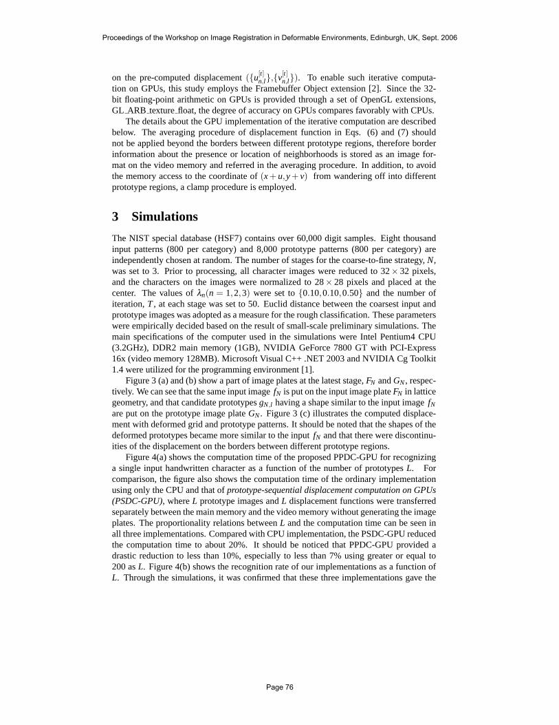
on the pre-computed displacement (u[t]n,l,v[t]

n,l). To enable such iterative computa-tion on GPUs, this study employs the Framebuffer Object extension [2]. Since the 32-bit floating-point arithmetic on GPUs is provided through a set of OpenGL extensions,GL ARB texture float, the degree of accuracy on GPUs compares favorably with CPUs.

The details about the GPU implementation of the iterative computation are describedbelow. The averaging procedure of displacement function in Eqs. (6) and (7) shouldnot be applied beyond the borders between different prototype regions, therefore borderinformation about the presence or location of neighborhoods is stored as an image for-mat on the video memory and referred in the averaging procedure. In addition, to avoidthe memory access to the coordinate of (x + u,y + v) from wandering off into differentprototype regions, a clamp procedure is employed.

3 Simulations

The NIST special database (HSF7) contains over 60,000 digit samples. Eight thousandinput patterns (800 per category) and 8,000 prototype patterns (800 per category) areindependently chosen at random. The number of stages for the coarse-to-fine strategy, N,was set to 3. Prior to processing, all character images were reduced to 32× 32 pixels,and the characters on the images were normalized to 28× 28 pixels and placed at thecenter. The values of λn(n = 1,2,3) were set to 0.10,0.10,0.50 and the number ofiteration, T , at each stage was set to 50. Euclid distance between the coarsest input andprototype images was adopted as a measure for the rough classification. These parameterswere empirically decided based on the result of small-scale preliminary simulations. Themain specifications of the computer used in the simulations were Intel Pentium4 CPU(3.2GHz), DDR2 main memory (1GB), NVIDIA GeForce 7800 GT with PCI-Express16x (video memory 128MB). Microsoft Visual C++ .NET 2003 and NVIDIA Cg Toolkit1.4 were utilized for the programming environment [1].

Figure 3 (a) and (b) show a part of image plates at the latest stage, FN and GN , respec-tively. We can see that the same input image fN is put on the input image plate FN in latticegeometry, and that candidate prototypes gN,l having a shape similar to the input image fNare put on the prototype image plate GN . Figure 3 (c) illustrates the computed displace-ment with deformed grid and prototype patterns. It should be noted that the shapes of thedeformed prototypes became more similar to the input fN and that there were discontinu-ities of the displacement on the borders between different prototype regions.

Figure 4(a) shows the computation time of the proposed PPDC-GPU for recognizinga single input handwritten character as a function of the number of prototypes L. Forcomparison, the figure also shows the computation time of the ordinary implementationusing only the CPU and that of prototype-sequential displacement computation on GPUs(PSDC-GPU), where L prototype images and L displacement functions were transferredseparately between the main memory and the video memory without generating the imageplates. The proportionality relations between L and the computation time can be seen inall three implementations. Compared with CPU implementation, the PSDC-GPU reducedthe computation time to about 20%. It should be noticed that PPDC-GPU provided adrastic reduction to less than 10%, especially to less than 7% using greater or equal to200 as L. Figure 4(b) shows the recognition rate of our implementations as a function ofL. Through the simulations, it was confirmed that these three implementations gave the


Page 76

(a) input image plate FN (b) prototype image plate GN

(c) displacement function with deformed gN’s

Figure 3: image and function plates in prototype-parallel displacement computation onGPUs

0

2000

4000

6000

8000

10000

12000

0 100 200 300 400 500 600

com

puta

tion

time

[mse

c]

number of prototypes, L

CPUPSDC-GPUPPDC-GPU

98.60

98.80

99.00

99.20

99.40

0 100 200 300 400 500 600

reco

gniti

on r

ate

[%]

number of prototypes, L

(a) computation time (b) recognition rate

Figure 4: total computation time and recognition rate using different number of prototypes


Page 77

(msec) CPU PSDC-GPU PPDC-GPUdisplacement computation 7400 1220 245

data transfer - 109 83plate image generation - - 90

others 98 98 90total processing time 7498 1427 508

Table 1: necessary time for respective processes in three implementations at L = 400.

same rates. The best recognition rate, 99.21%, was obtained with L=400, 500 and 600,which was superior to the result of simple matching without computing the displacement,96.5%, obtained in the rough classification.

Table 1 shows the necessary time for respective processes in three implementations.Compared with PSDC-GPU, it was clarified that PPDC-GPU could reduce the necessarytime for the displacement computation drastically. This result seems to confirm that thegeneration of image plates is useful for the efficient pipeline processing. However, theadoption of image plates could not considerably reduce the time for data transfer. Itshould be also noticed that the necessary time for generating the image plates resulted in90 msec and the sum of them, 173 msec, corresponded to 34% of the total processingtime.

4 Conclusion

In this study, we investigated speeding up a deformable approach to pattern recogni-tion. By considering the characteristics of GPUs and the deformable recognition ap-proach, prototype-parallel displacement computation on GPUs (PPDC-GPU) was pro-posed. Simulations were conducted based on the NIST handwritten database, and it wasclarified that the proposed implementation reduced the computation time to less than 10%compared with the ordinary implementation on CPUs.

In future tasks, we will investigate the generation of image plates on the video mem-ory instead of the main memory, since it is expected to eliminate the heavy data transferbetween the main memory and the video memory, and to generate the image plates morequickly with the fragment processor on GPUs. The video memories of the recent con-sumer graphic cards are getting larger and it seems to be possible to store the set of pro-totypes in the video memory. Another future task is the extension for three dimensionalobject recognition.

We intentionally kept the recognition method as simple as possible, since the mainproposes of this study were to show how to implement the deformable recognition ap-proach on GPUs efficiently and to clarify how much the GPU implementation could re-duce the computation time without degrading the accuracy, However, in order to obtainhigher recognition performance, it is essential to employ other procedures such as statis-tical classification and feature extraction [26]. Obviously, the dimensional reduction byfeature extraction is also helpful for saving the computation time.

Since handwritten character recognition is one of the most fundamental and importanttopics in the field of computer vision and pattern recognition, this study discussed thevalidity of the proposed method from its viewpoint. However the proposed framework can


Page 78

be widely applied to other problems, for instance, face recognition or object recognition.

Acknowledgement

This study was partially supported by JSPS Grants-in-Aid for Science Research (16700208).

References

[1] R. Fernando and M. J. Kilgard. The Cg Tutorial : the definitive guide to pro-grammable real-time graphics. Addison-Wesley, 2003.

[2] J. D. Owens, D. Luebke, N. Govindaraju, M. Harris, J. Kruger, A. E. Lefohn, andT. J. Purcell. A survey of general-purpose computation on graphics hardware. InEurographics 2005, State of the Art Reports, pages 21–51, August 2005.

[3] R. Yang and M. Pollefeys. Multi-resolution real-time stereo on commodity graph-ics hardware. In Proceedings of International Conference of Computer Vision andPatter Recognition, pages 211–217, 2003.

[4] J. Fung and S. Mann. Using multiple graphics cards as a general purpose parallelcomputer : Applications to computer vision. In Proceeding of International Confer-ence of Pattern Recognition, volume 01, pages 805–808, 2004.

[5] R. Strzodka, M. Droske, and M. Rumpf. Image registration by a regularized gra-dient flow - a streaming implementation in DX9 graphics hardware. Computing,73(4):373–389, 2004.

[6] U. Clarenz, M. Droske, and M. Rumpf. Towards fast non-rigid registration. InverseProblems, Image Analysis and Medical Imaging, AMS Special Session Interactionof Inverse Problems and Image Analysis, 313:67–84, 2002.

[7] K Moreland and E. Angel. The FFT on a GPU. In Proc. of SIG-GRAPH/Eurographics Workshop on Graphics Hardware, pages 112–119, 2003.

[8] J. Kruger and R. Westermann. Linear algebra operators for GPU implementation ofnumerical algorithms. In Proc. SIGGRAPH 2003, pages 908–916, 2003.

[9] J. Bolz, I. Farmer, and E. G. P. Schroder. Sparse matrix solvers on the GPU: Conju-gate gradients and multigrid. In Proc. SIGGRAPH 2003, pages 917–924, 2003.

[10] B. Widrow. The rubber mask technique – I. pattern measurement and analysis.Pattern Recognition, 5(3):175–197, March 1973.

[11] D.J. Burr. A dynamic model for image registration. In Proc. IEEE Comput. Soc.Conf. Pattern Recognition and Image Processing, pages 17–24, August 1979.

[12] M. Kass, A. Witkin, and D. Terzopoulos. Snakes: active contour models. Interna-tional Journal of Computer Vision, 1:321–331, 1988.

[13] R. Bajcsy and S. Kovacic. Multiresolution elastic matching. Computer Vision,Graphics, and Image Processing, 46(1):1–21, 1989.


Page 79

[14] A.L. Yuille. Deformable templates for face recognition. Journal of Cognitive Neu-roscience, 3(1):59–70, 1991.

[15] M. Lades, J.C. Vorbruggen, J. Buhmann, J. Lange, C.v.d. Malsburg, R.P. Wurtz, andW. Konen. Distortion invariant object recognition in the dynamic link architecture.IEEE-C, 42(3):300–311, March 1993.

[16] A.K. Jain, Y. Zhong, and S. Lakshmanan. Object matching using deformable tem-plate. IEEE Trans. PAMI, 18(3):267–278, March 1996.

[17] D.J. Burr. Elastic matching of line drawings. IEEE Trans. PAMI, 3(6):708–713,November 1981.

[18] T. Wakahara. Shape matching using LAT and its application to handwritten numeralrecognition. IEEE Trans. PAMI, 16(6):618–629, June 1994.

[19] A. Daffertshofer and H. Haken. A new approach to recognition of deformed patterns.Pattern Recognition, 27(12):1697–1705, December 1994.

[20] H. Sakoe, M. Masroor, and Y. Katayama. One dimensional-two dimensional dy-namic programming matching algorithm for character recognition. IEICE Trans.Inf. & Syst., E77-D(9):1047–1054, 1994.

[21] M. Revow, C. K. I. Williams, and G. E. Hinton. Using generative models for hand-written digit recognition. IEEE Trans. PAMI, 18(6):592–606, 1996.

[22] A.K. Jain and D. Zongker. Representation and recognition of handwritten digits us-ing deformable templates. IEEE Trans. PAMI, 19(12):1386–1391, December 1997.

[23] Y. Mizukami, K. Koga, and T. Torioka. A handwritten character recognition sys-tem using hierarchical extraction of displacement. IEICE, J77-D-II(12):2390–2393,December 1994 (in Japanese).

[24] Y. Mizukami and K. Koga. A handwritten character recognition system using hier-archical displacement extraction algorithm. In Proc. 13th Int. Conf. Pattern Recog-nition, volume 3, pages 160–164, 1996.

[25] R. March. Computation of stereo disparity using regularization. Pattern RecognitionLetters, 8(3):181–188, March 1988.

[26] Y. Mizukami. A handwritten Chinese character recognition system using hierar-chical displacement extraction based on directional features. Pattern RecognitionLetters, 19:595–604, 1998.

[27] Y. Mizukami, T. Sato, and K. Tanaka. Handwritten digit recognition by hierarchicaldisplacement extraction with gradual prototype eliminations. In Proc. 15th Int. Conf.Pattern Recognition, volume 3, pages 339–342, 2000.

[28] F. Glazer. Multilevel relaxation in low-level computer vision. Multiresolution ImageProcessing and Analysis, pages 312–330, July 1984.

[29] N. Yokoya. Dense matching of two views with large displacement. In Proceedingsof the 1st IEEE ICIP, volume I, pages 213–217, November 1994.


Page 80

INVITED TALK: ABSTRACT

Algorithms for Nonrigid Factorization

Andrew W. Fitzgibbon

Microsoft Research Ltd7 JJ Thomson AvenueCambridge CB3 0FB

England

[email protected]

http://research.microsoft.com/∼awf

Matrix factorization underpins several recent approaches to deformable object track-ing and modelling. In long sequences with occlusion, this factorization must be performeddespite missing data, a problem which has seen significant attention in recent computervision research.

Two classes of approach dominate the literature: EM-like alternation of closed-formsolutions for the two factors of the matrix; and non-linear optimization of both factors si-multaneously. As has been argued previously, nonlinear optimization based on a second-order approximation of the error function should be the faster approach. However alter-nation schemes remain enduringly popular.

I will show through theoretical and experimental arguments why this dicohotomy re-mains: it’s not just that lazy programmers don’t bother to implement second order meth-ods, but that alternation schemes often do well on “easy” problems, and that many prob-lems are “easy”. Secondly, one must take care that the second-order methods do not throwaway the nice properties of the alternation schemes. We introduce a class of hybrid algo-rithms which combine elements of both strategies, and show that these algorithms reachthe correct minimum more frequently and at reasonable speed.

Finally, I show that for some well-known structure-from-motion data, the global op-timum of the factorization problem does not, in fact, yield a realistic reconstruction. Toachieve a realistic result, Bayesian priors and robust error kernels must be introduced.This is pretty obvious; what is less obvious is that this further cements the advantage ofthe direct optimization approaches.


Page 81

deform’06 - proceedings of the workshop on image

Documents