UNCLASSIFIED

AD 631 848

DEADMAN ANCHORAGES IN VARIOUS SOILMEDI UMS

J.E. Smith, et al.

U.S.Naval Civil Engineering LaboratoryPort Hueneme, California

April 1966

Processed for...

DEFENSE DOCUMENTATION CENTERDEFENSE SUPPLY AGENCY

FOR FEDERAL SIENTIFIC AND TECHNIDL INFORMWAION

U. S. DEPARTMENT OF COMMERCE / NATIONAL BUREAU OF STANDARDS I INSTITUTE FOR APPLIED TECHNOLO

UNCLASSIFIED

*~ R434e''TechnicoI Report DEADMAN ANCHORAGES IN

.. VARIOUS SOIL MEDIUMS

April1 1966

BUREAU OF YARDS AND DOCKS

* ;~~\I/, ~ U. S. NAVAL CIVIL ENGINEERING LABORATORY

q Port Hueneme, California

Distribution c d" Aa- n is -cin -e

FOR FEDERAL SCIENTIFIC ANDTECHNICMd INFORMATION

ftrdeopy Wi~crof icheI

3~flJfl~EE (ppI

DEADMAN AtN'CHORAGES IN VARIOUS SOIL MEDIUMS

Technical Report R-434

Y-F015-15-01-010

by

.IJ. E. Smith and J. V. Stalcup

ABSTRACT

A test program was conducted to investigate deadman anchorage holdingcapacities under applied horizontal loads. Deadmen fabricated of concrete andranging in face area from 5 to 72 square feet were tested in depths of embedmentfrom ground level to 7 feet. The deadmen were pulled both singly and in groups ofthree, in sand and in two soils with cohesive characteristics. The test program alsoincluded tests on a model scale.

The applied load versus horizontal displacement relationship exhibited abasic recognizable farm for cdl conditions of tests. By graphic analysis, a seriesof reaction-pattern curves was developed relating deadman holding power in eachcohesive soil to thrse factors: deadman face area, depth of embedment, andwhether the deadmen were embedded singly or in a group. The results of the sandtests which were described in a previous report were converted from the previousanalysis to a compatible form and presented with the cohesive soil test results.These curves provide an empirical means for determining deadman holding capac-ities at different amounts of displacement within the range of conditions tested.

The investigation disclosed that multiple anchors develop a higher holdingcapacity per net area than a single deadman with the same total face area. Theincrease in holding capacity ranging from 5 to 209/6 depends upon such factors asdepth of embedment, the type of soil, and the spacing between deadmen. Undermost test conditions, up to a 30% increase in holding capacities was attained incohesive soils as compared to sand, but 2 to 3 times the horizontal displacementwas required to achieve the maximum holding capacity.

Distribution of this document is .nlimittd.

Copies available at the Clearinghouse (CFSTI) $3.00.The Laboratory invites comment on this report, perticlarly on the

results obtained by those who hove applied the information.

CONTENTSpage

I NTRODUCTI ON ......... ............................... I

TEST PROGRAM ............ ............................... 1

History ................................. I

Framework of Tests ........... ........................... 2

Description of Deadmen .......... ....................... 5

Soil Summary ............ .............................. 5

EQUIPMENT AND PROCEDURES ....... ....................... 11

Full-Scale Test Apparatus ......... ....................... I I

Full-Scale Test Procedures ........ ....................... 11

Model Test Apparatus ......... .......................... 19

Model Test Procedures .......... ......................... 21

RESULTS ............. .................................... 24

General ............. ................................ 24

Analysis ............. ................................ 24

DISCUSSION ............ ................................. 30

Application of Results ......... .......................... 30

Computer Program Potential ........ ....................... 40

CONCLUSIONS ............. ............................... 41

ACKNOWLEDGMENT ........... ............................ 41

APPENDIXES

A - Observed Data Points and Empirical Curves for theFull-Scale Tests ......... .......................... 42

B - Mathematical Analysis ............................... 58

REFERENCES ............. ................................. 70

INTRODUCTION

The use of deadman anchorages to provide lateral support for structures suchas quay walls is an accepted engineering practice. High quay walls must remainverticai for ship-docking purposes while containing and supporting large quantitiesof fill material behind them on the dockside. Theoretical computations for theholding power of deadmen generally are based on equivalent fluid pressure or onan assumed failure of a soil mass along a shear plane. But the theories do notreadily account for the ioad-•cV.olacement characteristics of deadmen.

The U. S. Naval Bureau of Yards and Docks sponsored an investigation,Task No. Y-F015-15-01-010, conducted by the U. S. Naval Civil EngineeringLaboratory at Port Hueneme, California, to determine deadman reactions underapplied horizontal loads. The investigation has encompassed three separate phasesof testing. In Phases I and 2, full-scale tests were conducted in sand in whichdeadmen were pulled singly and in rectilinear groups of three; the results werepreviously reported. 1,2 In Phase 3, full-scale tests were conducted in two cohesivesoils with test conditions similar to those in sand; model tests were included. Thisreport describes the overall investigatiun; the results obtained from the cohesivesoil tests are presented along with the results previously obtained in the sand tests.

TEST PROGRAM

History

The three separate test phases of deadman anchorages were conducted atintermittent times over a period of years. Phase I included tests of two sizes ofdeadmen in sand and in depths to 3 feet. Subsequently, Phase 2 included tests ofdeadmen of seven sizes in various depths to 7 feet. The results of the Phase 2 testswere combined with those of Phase 1. By means of computer programming, aregression analysis of the data was performed and an empirical equation was devel-oped relating holding power at specific horizontal displacements to three variables:depth, face area, and whether the deadmen were single or in a group of three. Bymeans of a nomograph based on this equation, it was possible to rapidly determinedeadman holding capacities for different amounts of horizontal deadman displacementsin sand. 2

The encouraging results obtained from the deadman tests in sand promptedPhase 3 of the program in which deadmen were tested in soils with cohesive charac-ieristics. The intent was to combine and analyze the results of all three phases ina manner that would enable the accurate determination of deadman holding powersat various displacements, while considering such variables as soil characteristics inaddition to the variables which were accounted for in the prior programs. To thisend, Phase 3 was designed so that a minimum number of tests could be integrated withthe previous tests to give a maximum amount of information. In addition, model testswere incorporated into the third phase for two purposes: first, to investigate thevariables affecting deadman performance over a wider range of conditions than waspractical to investigate on a full scale; and second, to investigate the effect ofadditional variables not practical to investigate on a full scale.

Framework of Tests

Full-Scale Tests. Fifty-seven full-scale tests were included in the programcovered by this report. Each test represented a separate set of conditions relating tosuch factors as soil type, depth of embedment, face area of deadman, and whetherthe deadmen were pulled singly or in multiples of three. An outline of the full-scaletests in a classified order is presented in Table I. The test numbers represent a !ogicalorder for classifying the tests. The sequence of the tests as actually conducted wasdifferent and extended over a considerable period of time.

Thirty-three of the full-scale tests were conducted in sand, 12 in sandy silt,and 12 in silty sand (Table I). An irregular variety of deadman sizes, depths ofembedment, and spacings was used to envelop the range of conditions investigated insand (Phases 1 and 2). This irregularity resulted because Phases 1 and 2 initially wereindependent programs whose results were subsequently combined when computer anal-ysis wn• undertaken. The cohesive soi! testing (Phase 3) was planned with results ofthe sand tests considered as a base and with computer programming in mind. Conse-quently, a more efficient coverage of the variables was possible. In Phase 3, deadmenof three sizes were pulled singly at depths of 0, 3, and 6 feet, and deadmen of onesize were pulled in multiples of three at these same depths in the two cohesive soils.

Model Tests. The model tests were comprised of two parts. First, all 57

full-scale tests were duplicated on a scale of I to 18. The intent was to obtain acomparability factor that would permit a reliable determination of deadman anchorageperformance from model tests. Second, 37 additional tests (termed extra-variable tests)were conducted for the purpose of studying the variables of the full-scale tests over awider range and for investigating additional variables not included in the full-scaletests. Table II lists the 37 extra-variable model tests that followed the first 57 tests.The purpose of each of these tests is indicated in the Shape and Spacing columns ofTable II. In general, the effect of and limits for spacing multiple deadmen, the

effect of shape and perimeter of deadmen, and the effect of odditonni nao;sture in thecohesive soils were the additional variables included in the extra variable model tests.

2

Table I. Outline of Full-Scale Tests

Single Deadman Multiple Deadmen

Test Face Area Det 1 Ts ae Area?. 1 Depth £T Spacing/No. (sq ft) (ft) . No. (sq ft) I (ft) (f t)

Sand: Phases 1 and 24/

1-6 5 G L, 1,213,5,7 27 33 4 6.57 9 6 28-30 54 GL,2,4 3.58-11 10 GL,1,2,3 31-33 60 GL,2,4 2.012,13 11 4,614 17 615-21 20 G L, 1,2,2,3,4,622,23 45 GL,224-26 72 G L,2,4

Sandy Silt: Phase 3

34-36 13.5 G L,3,6 43-45 27 G L,3,6 4.537-39 27 G L13,640-42 54 G GL3,6

Si Ity Sand: Phase 3

46-48 13.5 G L.,3,6 27 G L,3,6 4.549-51 27 G L,3,652-54 54 G Iv,3,6

I/ GL = ground level2/ The face area includes the total face area of three single deadmen; e.g., 33

indicates three deadmen, each with a face area of 11 square feet.3 Distance between deadmen in multiple-deadman grouping.4/Tests 8-11, 15-17, and 19 are Phase 1; all others are Phase 2.

3

Table II. Outline of Model-Scale Extra-Variable Tests!-/

Single Deadman Multiple Deadmen

Test Face Area Depth-'j a3 Test Face Area Depth2J SpacingNo. (sq ft) (ft) ape r Jo. (sq ft) (ft) (ft)

Sand

58-60 17 G L,2,4 OR D 67,68 33 4,4 3.75,5.25

61-64 20 GL,GL,2,2 /_D•sQ, Z

65,66 27 2,2 O,A

Sandy Silt

69-71 13.5 GL,3,6 [o[p 76-78 27 GL,3,6 3.00

72-75 27 GL,3,GL,3 OQ 79,80 27 GL,3 6.00

Silty Sand

81-83 13.5 G L,3,6 [IIJ 188-90 27 GL,3,6 3.00

84-87 27 GL,3,GL,3 0,Q ,L, 91,92 27 GL,3 6.00

Sandy Silt With Extra Moisture

93 J 27 J3 j _C L I __Silty Sand With Extra Moisture

I94I 1 1 1I

SAll fu;l-scule tests outlined in Table I were duplicated on a model scale in addition tothe model-scale extra-variable tests outlined in Table II.

2j GL = ground level

3_/ Shape symbols are as foi lows:Rectangle on endRectangle on sideRoundTriangle

4

Description of Deadmen

Full-Scale Specimens. All of the full-scale specimens were constructed ofreinforced concrete. Table III summarizes their dimensions, weights, and face areas;most of them were 3 feet high. With two exceptions, the deadmen were designed sothat a steel coupling pad could be attached with four bolts. The pad was designedso that a coupling elevation of 0.3 h or 0.4 h could be achieved depending upon theorientation of the pad, where h is the specimen height and the coupling elevation isthe location of applied force on a vertical axis of deadmen measured from the bottom.Figure 1 shows representative deadmen used in the tests; the coupling pad may benoted. The 10- and 20-square-foot deadmen tested in Phase 1 were designed witha vertical slot in their faces (Figure 2) so their behavior with various coupling eleva-tions could be studied. It was determined in Phase 1 that maximum holding powercould be attained with the coupling elevation at 0.3 h for ground-levei testsand 0.4 h for all tests at greater depths. I This criterion was used for all subsequenttests.

The deadmen which were 20 squcre feet in face area and smaller had onecoupling; larger specimens had two or three couplings (Figure 1).

Mode! Specimens. The model specimens were shaped from blocks of redwoodand were sanded to a smooth but not fine finish. Their dimensions corresponded tothe full-scale specimens on a scale of 1 to 18. Round and triangular models were-!sc irc !uded.

Soil Summary

The full-scale and model tests were conducted in three soils: sand, sandysilt, and silty sand (Figure 3). The identifications are based on the U. S. ArmyCorps of Engineers system for describing soils. 3 Table IV lists the characteristics ofthe soils used in the test programs.

The sand was natural beach sand found at the NCEL beach test locatior.. The

sandy silt was imported in the dry season from the bottom of a small inland reservoirbasin. One-thousand cubic yards of material wcs transported to the test site and

utilized as explained under Equipment and Procedures. The silty sand was obtainedby blending the sand and the sandy silt. The characteristics of the soils in the full-scale and model tests were maintained as nearly identical as possible. However,because of necessarily different methods of handling and compaction, slight differences

in characteristics did result as indicated in Table Ill.

5

I II II II I I I mmmm nmunmmmm • m,,mI

Table Ill. Deadman Anchorage Sizes

Dimensions . A .Face Area - I ... Approximate Weight,/

(sq ft) Width j Height Thickness j(Ib)(ft) (ft) (in.)

Prototype and Model!/

5 2.50 2.00 12 1 730 -

9 3.00 3.00 12 1,32010 3.54 2.83 10 1,225112/ 3.75 3.00 12 1,47013.5 4.50 3.00 12 2,310172/ 5.63 3.00 12 2,90020 6.67 3.00 12 3,43020 5.00 4.00 10 2,86027 9.00 3.00 12 4,60045 15.00 3.00 2 8,4o0054 18.00 3.00 12 10,00072 24.00 3.00 12 13,200

Model Only

20 Round, D = 5.05 12 not applicable20 Triangle, W 682 12 not applicable

H = 5.90

27 Round, 0 = 5.86 12 not applicable27 Triangle, W = 7.90 12 not applicable

_ _ _ _ _ _ _ _ _ -__

1/ Models were 1-to-18 scale.2/Nominal face area.

SWeights do not apply to models.

6

ISE-

Ilkk

Figure 1. Representative deadnren after use in test programs.

7

'I

0)C

0

�00

-c4-

Ca

00

CJ

0I-

0)

8

001 1 - -*'

- -

V06.

4

t-- m-4

90

10

'I

00

Lo'

I2 - Ii T

IiDOI

Lw (O 00

C- D

L6FV) 0 1

""0 (Y) 0 0 to

-~I =~ ON C (N -n

C) I0 I I ! C4 0 U

-0 0

E "¼ >.JC NL, ~ U

E ,--- 0 CV0

-) o 4 ,4'

ItU OD Cl OD U9008 C) (N

4--*t -II

0 C')'

_ ~ 0

_ U)

U) -I . 0% I

a-

10

EQUIPMENT AND PROCEDURES

Full-Scale Test Apparatus

The general layout of the apparatus used is shown in Figure 4. Essentially,the test facility consisted of a 20-foot-gage railway about 250 feet long. A railcart and a BU-140 Type M two-drum winch were anchored se,'urely at one end ofthe railway, and the site of embedment, an area about 75 feet wide by 100 feetdeep, was at the other end. For tests in sandy silt and silty sand, a U-shapedenclosure 54 feet wide by 72 feet long was constructed to contain the imported soil(Figure 5). The winch applied the load to the rail cart through a six-part line, andthe rail cart in turn was connected to the deadmen; for some of the very high-capacitypulls, it was necessary to two-part the dead end of the six-part line. A wire-ropeattachment was used in the tests of the single smaller deadmen. Multiple wire-ropeattachments were used with a spreader-bar arrangement (Figure 5) in tests of multipledeadmen and in tests of single deadmen 9 feet wide or wider. Chains up to 2-3/4-inchsize were incorporated in the apparatus in lieu of wire ropes when especially highloads were anticipated. A horizontal pull was maintained on the deadmen by passingthe loading wire rope through a looped bar attached to a 20,000-pound concreteweight (Figure 6). The weight was buried in the sand more than 120 feet from thedeadmen so that the vertical component at the weight would be relatively minor andnot raise the weight.

Applied loads were measured by means of a dynamometer placed in the linebetween the rail cart and the deadmen at a point where friction would not affect thereading (Figure 7). For somie high-capacity pulls it was necessary to place twoinstruments in parallel to obtain the maximum readings. A 100,000-pound-capacityBaldwin Type D SR-4 load cell and two specially fabricated 400,000-pound-capacitydynamometers were used interchangeably as appropriate according to anticipated loads.

Full-Scale Test Procedures

Phases I and 2: Tests in Sand. The procedures for some of the 33 tests in sandreported here varied somewhat because two separate phases of testing were involved;however, the basic principles of the tests were maintained, and an examination ofthe data indicated that the effects on the net results were negligible. The test numbersthat apply to each phcse are identified in Table I.

Preparation for each test consisted of excavating sand within the embedmentarea, positioning the anchorage(s), and backfilling the sand to a prescribed depth(Figures 8 and 9). In the tests involving multiple deadmen, three deadmen werealigned in rectilinear groups of three perpendicular to the direction of pull (Figure 10).Depth was controlled by altering the overall elevation of the ground surface. Thebackfill was compacted by applying fresh water for a prescribed length of time onceduring and once again upon completion of backfilling.

11

.4-0I-

0"I-U,4,

.0-a,0

U

U-

4)L.

LL

7-�* �

I.

12

Figure 5. Cohesive soi containment area.

13

Figure 6. Twenty-thousand-pound concrete weight used to maintainhorizontal pull.

14

0-

CL0

0)

0)LL

15

Figure 8. Positioning deodman anchorage.

16

Figure 9. Backfi I I ng around deadman anchorage.

Figure 10. Multiple deadman anchorages positioned for test.

17

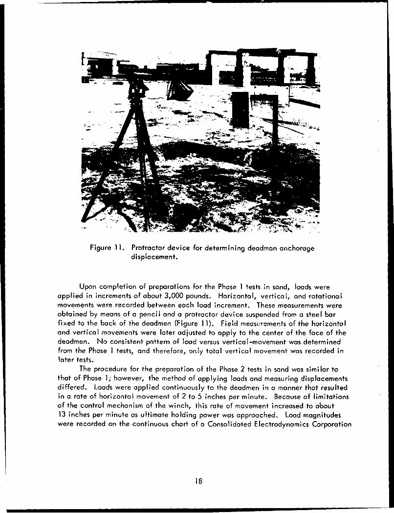
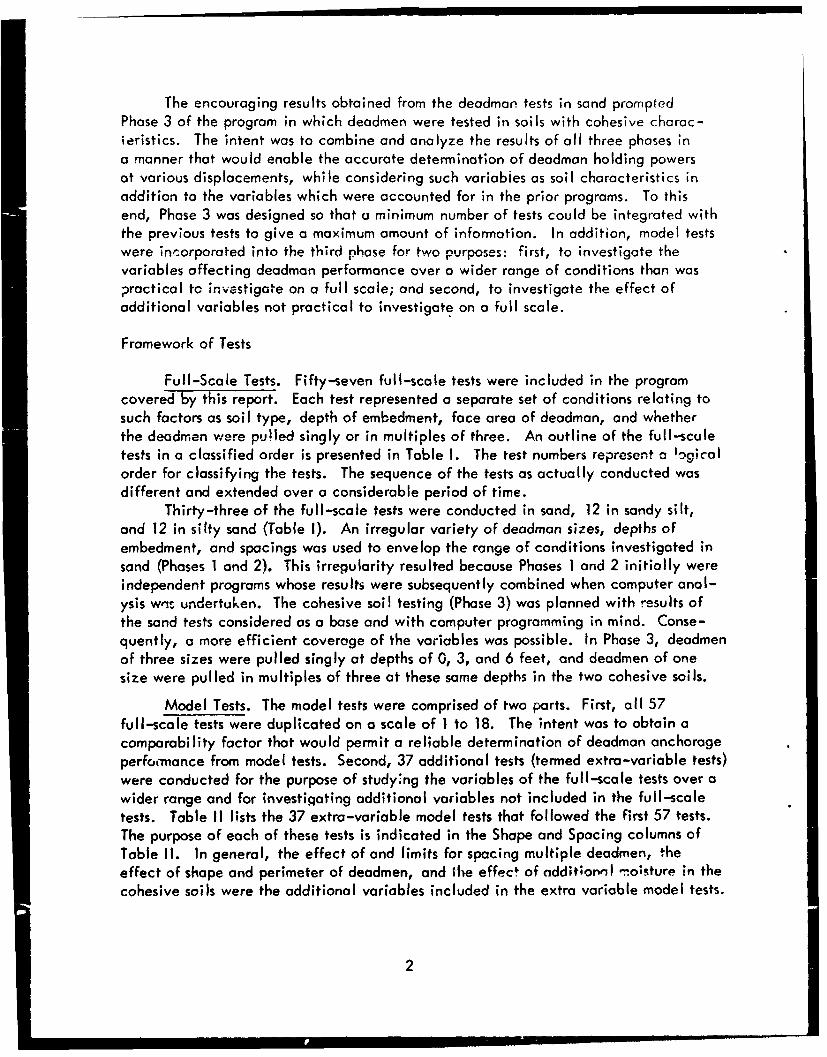
Figure 11. Protractor device for determining deadman anchoragedisplacement.

Upon completion of preparations for the Phase 1 tests in sand, loads wereapplied in increments of about 3,000 pounds. Horizontal, vertical, and rotationalmovements were recorded between each load increment. These measurements wereobtained by means of a pencil and a protractor device suspended from a steel barfixed to the back of the deadmen (Figure 11). Field measurements of the horizontaland vertical movements were later adjusted to apply to the center of the face of thedeadmen. No consistent pattern of load versus vertical-movement was determinedfrom the Phase I tests, and therefore, only total vertical movement was recorded inlater tests.

The procedure for the preparation of the Phase 2 tests in sand was similar tothat of Phase 1; however, the method of applying loads and measuring displacementsdiffered. Loads were applied continuously to the deadmen in a manner that resultedin a rate of horizontal movement of 2 to 5 inches per minute. Because of limitationsof the control mechanism of the winch, this rate of movement increased to about13 inches per minute as ultimate holding power was approached. Load magnitudeswere recorded on the continuous chart of a Consolidated Electrodynamics Corporation

18

oscillograph in conjunction with a Model 1-113 carrier amplifier. Correspondinghorizontal displacements were also recorded on the chart. These measurements wereobtained by means of a flexible rod extending to a helipot 10,000 ohms potenti-ometer secured in open ground 10 to 15 feet back of the deadmen (Figure 12). Atthe conclusion of each test pull, the total vertical displacements were measured.On the occasions when the deadmen were exposed sufficiently, total rotationalmovements were also obtained.

Soil samples were obtained periodically throughout both sand-test phases toestablish and define the standard sand condition and to verify ,;:ceptable uniformityof sand conditions. The samples were obtained at different locations and depths inthe areas affected by displacement of the deadmen. Moisture content and wet anddry densities were determined. The mechanical analysis was unnecessary after theinitial samples because variations in sand gradient were negligible.

Phase 3: Tests in Sandy Silt and Silty Sand. Procedures for applying loadsand obtaining measurements in the Phase 3 tests were the same as described for thePhase 2 tests. Also, preparations were similar through backfilling and compactingthe soil. For each test, the cohesive soil within the entire area affected by themovement of the anchorage(s) was excavated. The deadmen were then carefullypositioned so their face areas were perpendicular to the direction of pull, and sothe coupling elevation was at the necessary height to allow a horizontal pull.Backfilling to the prescribed depth was done in 18-inch layers. The desired mcisturecontent and compaction required for uniformity was achieved by sprinkling the areawith fresh water a prescribed length of time for each layer and then making fourposses with a 6-ton caterpillar tractor (Figure 13). For the cohesive soils, sampleswere obtained for each test at 1-, 3-, and 5-foot depths at random locations in thesoil area affected by deadman displacements. Moisture content and wet and drydensities were measured. The procedure followed for preparing the soils resulted inreasonably uniform conditions with regard to all tests. Average values obtained arelisted in Table IV. Three triaxial shear tests for each of the two cohesive soils wereconducted on the samples taken at random times throughout the test!ng. The resultsof the three tests agreed within 101% and the average cohesion values determinedfor each soil (Table IV) were considered to be valid.

Model Test Apparatus

The model apparatus (Figure 14) was designed and constructed to duplicatethe full-scale facility as closely as practicable. A scale of 1 to 18 was selectedto reduce the model tests to laboratory dimensions.

19

Figure 12. Potentiometer on open ground behind deodmon anchorage.

Figure 13. Compacting cohesive soil.

20

Figure 14. Model test apparatus.

The model was assembled on a 3-foot 8-inch by 8-foot table. A small winchpowered by a 1/4-horsepower electric motor was mounted on one end of the table.At the opposite end, the soil was contained in a 3- by 3-foot area with a 1-foot-high buttress constructed of 1/2-inch-thick plywood at the back and 1/2-inch-thickplastic glass at the sides. The area was open on the side toward the center of thetable. To avoid the possibility of the soil mass sliding on the bottom, 1/4-inchstrips of wood were tacked onto the bottom of the containment area crosswise to thedirection of pull. Behind the soil-containment area, a platform was constructed forthe support of three potentiometers used to measure the horizontal displacements ofthe model deadmen.

Model Test Procedures

The procedures for the model tests were essentially the same for all three typesof soil and corresponded to the procedures used for Phases 2 and 3 of the full-scaletests. The model deadmen were embedded in the soil in the containment area andpositioned relative to the winch so that the applied loads would be perpendicular fodeadman face areas and level with coupling elevations. The soil then wcs bac.kfilled

21

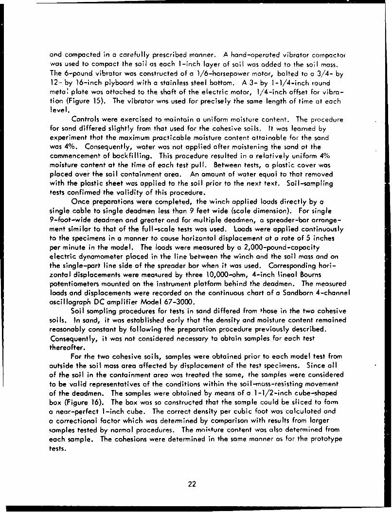
and compacted in a carefully prescribed manner. A hand-operated vibrator compactorwas used to compact the soil as each 1-inch layer of soil was added to the soil mass.The 6-pound vibrator was constructed of a 1/6-horsepower motor, bolted to a 3/4- by12- by 16-inch plyboard with a stainless steel bottom. A 3- by 1-1/4-inch roundmetal plate was attached to the shaft of the electric motor, 1/4-inch offset for vibra-tion (Figure 15). The vibrator wns used for precisely the same length of time at eachlevel.

Controls were exercised to maintain a uniform moisture content. The procedurefor sand differed slightly from that used for the cohesive soils. It was learned byexperiment that the maximum practicable moisture content attainable for the sandwas 4%. Consequently, water was not applied after moistening the sand at thecommencement of backfilling. This procedure resulted in a relatively uniform 4%moisture content at the time of each test pull. Between tests, a plastic cover wasplaced over the soil containment area. An amount of water equal to that removedwith the plastic sheet was applied to the soil prior to the next text. Soil-somplingtests confirmed the validity of this procedure.

Once preparations were completed, the winch applied loads directly by asingle cable to single deadmen less than 9 feet wide (scale dimension). For single9-foot-wide deadmen and greater and for multiple deadmen, a spreader-bar arrange-ment similar to that of the full-scale tests was used. Loads were applied continuouslyto the specimens in a manner to cause horizontal displacement at a rate of 5 inchesper minute in the model. The loads were measured by a 2,000-pound-capacityelectric dynamometer placed in the line between the winch and the soil mass and onthe single-part line side of the spreader bar when it was used. Corresponding hori-zontal displacements were measured by three 10,000-ohm, 4-inch lineal Bournspotentiometers mounted on the instrument platform behind the deadmen. The measuredloads and displacements were recorded on the continuous chart of a Sandborn 4-channeloscillograph DC amplifier Model 67-3000.

Soil sampling procedures for tests in sand differed from those in the two cohesivesoils. In sand, it was established early that the density and moisture content remainedreasonably constant by following the preparation procedure previously described.

Consequently, it was not considered necessary to obtain samples for each testthereafter.

For the two cohesive soils, samples were obtained prior to each model test fromoutside the soil mass area affected by displacement of the test specimens. Since allof the soil in the containment area was treated the same, the samples were consideredto be valid representatives of the conditions within the soil-moss-resisting movementof the deadmen. The samples were obtained by means of a 1-1/2-inch cube-shapedbox (Figure 16). The box was so constructed that the sample could be sliced to forma near-perfect 1-inch cube. The correct density per cubic foot was calculated anda correctional factor which was determined by comparison with results from largersamples tested by normal procedures. The moisture content was also determined fromeach sample. The cohesions were determined in the same manner as for the prototypetests.

22

Figure 15. Compacting soil for model test.

N-

Figure 16. Model test facility soil-sampling tools.

23

RESULTS

General

The applied load versus horizontal displacement relationship, herein referredto as the deadmar anchorage reaction pattern, represents the primary data desiredfrom the tests on which this report is based. The reaction patterns observed for allfull-scale and model tests exhibited a basic recognizable form, but with a consid-erable range of variation. Typical configurations of the basic form are shown inFigure 17. As load was applied to single or multiple deadman anchorages, they firstwould adjust to a condition of equilibrium before finite motion occurred. Then thedeadmen would move in the direction of pull in a creeping uneven fashion. The netresult of this uneven motion, however, was a smooth even record of displacement forthe deadmen as a whole. Initial movements were so small that they could not beaccurately measured and can reasonably be assumed to be negligible. Consequently,the deadmen essentially remained immobile until a breakaway load was reached(ko, Figure 1N). At this load, measurable anchorage movement occurred at anever-increasing rate as the load increased until the maximum attainable load wasreached. Here the load record would begin to undulate and gradually drop off.Tests were terminatea before deadmen were pulled out of the ground, but it wasbelieved that this would be the eventual result with continued pull.

Verticcl and rotational movements in sandy silt and silty sand are comparableto those in sand. Their effect on and relation to deadman holding capacities appearedto be negligible. The total vertical movement at the termination of each pull rangedfrom 0 to 5 inches regardless of the dlipth and size of the deadman. The rotationalmovement, when obtained, also showed a random variation between rotation forwardsand backwards. Total rotation was always less than 4 degrees.

The extent of the soil mass affected by displacement of deadmen in bothcohesive soils in the full scale was indicated by a slight to pronounced bulging atthe surface depending on the depth of embedment (Figure 18). As nearly as couldbe determine,-, the extent of the soil mass forward of the deadman that was mobilizeddue to deadman movement was equal to about 1-1/2 times the depth to the bottom ofthe deadman (Figure 19). Similarly, the extent of the mobilized soil mass to eachside of the deadman Xue to its movement was approximately equal to half the depthto the bottom of the deadman. On the model scale the definitions of affected soilmass were more clear. The same criterion for the extent of affected soil mass appliedon the model scale as on the full sale.

Ana lysis

. Computer Approach. A computer programming approach to analysir wasattempted first. The development and present status of the computer program isdescribed in Appendix B. It was believed that the influence of some or ail oi ;he

24

following variables on deadman performance and their interdependence might bedefined in equation form: (1) depth of embedment, (2) height of deadman, (3) widthof deadman, (4) multiple versus single deadmen, (5) height t width ratio of deadman,(6) perimeter of deadman, (7) cohesion of the soil, and (8) density of the soil.Further, it was believed that by testing on a model scale, the same variables mightbe investigated over a greater range and that the influence of the following additionalvariables might be determined: (1) the most effective spacing of deadmen at variousdepths for multiple pull effect, (2) the limits for spacing deadmen at various depthsfor multiple pull effect, (3) the most effective shape for single deadmen, and (4) theeffect of excess moisture content on cohesive soils.

Two steps toward successful computer program analysis were accomplished. Abasic equation was developed that accurately fits a smooth curve through observeddata points defining the deadman reaction pattern for each individual test in all threesoils. Also, it was determined that a good comparability factor exists between thefull-scale and model test results. However, the nature of a computer program analysiseffort encompassing the numerous variables mentioned is that of successive trials andadjustments. Satisfactory determination of deadman anchorage performance anddefinition of the effects of the variables by computer analysis were not achieved.Thus, it was not possible to obtain meaningful computer results for this report nor toutilize the model test results. It is important to emphasize that the computer programanalysis previously reported 2 for tests conducted only in sand remains valid, and infact, is used to supplement the graphic procedure that is described next. Computerprogramming for the sand phases was more successful because fewer variables wereinvolved, and also the reaction patterns proved more compatible throughout therange of test conditions.

Graphic Procedure. When it became evident that the computer programanalysis combining results of tests in all three soil types was not promising, testresults were examined separately by soil type. A graphic analysis of the full-scaletest results in cohesive soils was undertaken. It was not necessary to include thesand tests in the graphic procedure. These were the same tests encompassed by theearlier test phases previously reported. 2 The prior sand-test computer analysis isvalid and can be used. For this report, the sand-test results analyzed earlier werereconstructed to a form compatible with the cohesive soil results so that directcomparisons could be made.

For practical reasons, the graphic analysis of the cohesive soil tests cannotaccount for the influences of all of the variables that were meant to be analyzed bycomputer. Instead, it defines the deadman reaction patterns for the tests in cohesivesoils correlating three variables: (1) depth of embedment, (2) face area, and(3) whether the deadmen were pulled singly or in multiples of three.

25

EE

-00

0

N~0.

0 a

0~0

0 0 0

si.)po -

26.

0v,

E

co

J 4

270

100,

.000

1-/

--- ------- ......... .0 .. .. .*1***'**'*. ..... ..... .. .... .

%I ..... . ... .................. ........... .....e % ... ... ... ... ......

.. .. . .. . ./.

Det

Figure ~N 19/prxmt xeto olms mblzdb oiotldslcmnof eadon

28 --

The observed data points recorded for all of the full-scale tests in the cohesivesoils and the curves graphically determined to fit them are shown in Figures A-1 toA-14 of Appendix A. Figure A-15 presents an example of the observed data pointsrecorded for three of the tests conducted in sand together with the curves calculatedto fit them by means of the equation previously developed from the sand tests. Com-prehensive data for the model and full-scale tests are presented in Table B-1 ofAppendix B.

In large measure, the results of the first step in the graphic analysis are shownin Appendix A. Three important factors were taken into account in achieving theempirical curves shown for the deadman anchorages in the cohesive soils. First,because of the difficulty in measuring initial small increments of movement of thedeadmen, it was known that the maximum holding powers, P(max), measured(Figure 17) were the most accurate and reliable data points. Consequently, theP(max)'s were used as the starting points for graphing each curve. Second, thebasic deadman reacti-•, nattern was known from the overall results. In some tests,load readings at small in:rements of movement were erratic and lower than theyreasonably should be. Therefore, the basic reaction pattern proceeding from theP(max)'s was permitted to override the lower observed load readings for smallincrements of movement. Third, for multiple deadmen, reaction patterns werecompared with those single deadmen having similar total face areas, and theincreased holding-power effect of the multiple pull as determined for sand 2 wastaken into account.

Once the initial curve fits for each individual test were achieved on the basisdescribed, groups of tests of deadmen with identical face areas were plotted, andproportional adjustments were made on the basis of depth. Likewise, groups of testsof deadmen embedded at the same depth were plotted, and proportional adjustmentswere made on the basis of face areas. By several successive adjustments, the graphsas presented in Appendix A were completed. Figures A-1 to A-3 illustrate theempirical curves arrived at for deadmen with identical face areas at different depthsin sandy silt. Figures A-4 to A-6 illustrate the empirical curves for deadmen withdifferent face areas at the same depth in sandy silt.

Upon completion of the curves shown in Appenoix A, further analysis wasnecessary to convert the information into "design graphs. " The development ofdesign graphs was achieved by a process similar to that described for the developmentof the curves in Appendix A. However, this time it was possible to use a more directplotting method because the i"regularities and inconsistencies in portions of thereaction patterns for all the tests hod been corrected in the earlier process used forthe curves in Appendix A. The first step was to plot the maximum holding power,P(max), versus face area for the different depths in each type of soil. These "analysis"graphs are shown in Figures 20, 21, 22, and 23. Smooth curves were drawn givingweight to the data points primarily according to depth and face area with secondaryconsiderations given to soil type. Then new data points on the" curves coinciding withthe face areas desired for the design graphs were determined. From these data points

29

the design graphs for the cohesive soils were developed (Figures 24 through 27).Again because the maximum holding power is the most reliable reference point,P(max) was used as the starting point for each curve. From here the curve couldbe drawn accurately to the ko point by comparison with previous curves in the samesoil type that exhibited a P(max) close to the same value.

To complete the comparisons of deadman holding powers in the three soil typescovered by this report, corresponding design graphs were drawn for the sand condition(Figures 28 and 29). These were obtained by plotting the reaction patterns of dead-man anchorages using the graph of average holding power of deadmen in sand previouslydeveloped and reported. 2 Figure 28 shows the reaction patterns for single deadmen offour face areas (10, 20, 40, and 60 square feet) embedded at three depths in sand:ground level (GL), 3 feet, and 6 feet. Figures 24 and 25 give the reaction patternsfor the same four sizes of single deadmen at the same three depths in sandy silt andsilty sand. These sizes and depths were selected because they are practicable fordesign application and they offer a reasonable range for interpolation.

Figures 26, 27, and 29 show the reaction patterns for multiple deadmen of twoface areas (40 and 60 square feet) embedded at three depths (ground level, 3 feet,and 6 feet) in sandy silt, silty sand, and sand respectively. The two face-area sizesused in developing these graphs are considered to encompass the practicable designranges covered in the test programs.

Use of the design graphs for single deadman design is self-evident. The holdingpowers per particular displacements for a particular size of deadman can be interpo-lated from the graph representing the type of soil of interest. Use of the design graphspertinent to multiple deadmen is similar, but it must be kept in mind that the faceareas listed represent the aggregate total for the number of deadmen used; for example,if three deadmen of 20 square feet each are used, the face area to use in referring tothe graph is 60 square feet.

DISCUSSION

Application of Results

The test results may be considered valid for those conditions encompassed bythe test program. These conditions are (1) the types of soils described, (2) depthsof embedment from ground level to 6 feet, (3) deadman face areas from 5 to72 square feet, and (4) spacing distance of multiple deadmen within the range of0.6 h and 1.7 h. Interpolation within the range of conditions represented by thegraphs can give characteristic deadman reaction patterns under applied loads notreadily determined by analytical means.

30

700

Depth (ft)

600

500

400

ao.

300

200 G

100GLtsdaapis

(0 Data points for developing Figure 24- Fitted curves for test results at GL,

3-ft, and 6-ft depths

0 10 20 30 40 50 60Face Aruz (sq f t)

Figure 20. Analysis graph: maximum load versus face area for singledeodmen in sandy silt.

31

700

600 O_.Lepth (ft)

600

A• GL test data points

e 3-ft test data points

0l 6-ft test data points

S00 0 Data points for developing Figure 25

- Fitted curves for test results at GL, 3-ft,and 6-ft depths

400

U3a.

300

200

100

00 10 20 30 40 50 60

Face Area (sq ft)

Figure 21. Analysis graph: maximum load versus face area for single

deadmen in silty sand.

32

700

600j

A GL test data points

e l.ft test data pointsE] 6-ft tesT into points o<

500 (D Data points for deve!oping Figure 26-Fitted curves for single d*Qi'.omn test results )0

-- Curves adjusted to represent GL and 3-ft

400 .0

300

20 ____e

300 OF_____00_

000

10 / 10 2 04 06

Face Area ( sq ft)

Figure 22. Analysis graph: maximum load versus face area for multipledeodmen in sandy silt.

33

700

600

AGL test data points

G3-ft test data points06-ft test data points

500 Data points for developing Figure 27500 - Fitted curves for single deadman test results

at GL, 3-ft, and 6-ft depths

-- Curves adjusted to represent GL and 3-ftdepths for multiple deadmen3

4000

00

300000

200 GL__

100

0 60 10 20 30 4P50 6

Face Area (sq ft)

Figure 23. Analysis graph: maximum load versus face area for multipledeadmen in silty sand.

34

n n | b w,

64O 1Foe* ArM (sq ft) Depth (ft)

I-1 60Z• 40 =,.......4 6

0 20/

/,

400 " ,

480 ! -- -- •'0

"-" 320

2,0 / ¢ ;,,,. • ,•

8O

0 '

0 4 8 12 16 20

rlorisonte! Displo©ement (in.)

Fif•ure 24. Desig. graph: load versus horizontal displacement for singledeodmen in sandy sl It.

35

ill • iliilm ann i mum n mama== ....

640 _______________ _ _ _

Face Area (sq ft)0 60040 Depth (ft)A 20

560 010 6

480

6

400_____________ _______ _

3aI

A 3

6

GLso6

GL

Depth is to topedge of deadman

0 4 812 16 20Horizontal Displacement (in.)

Figure 25. Design groph: load versus horizontal displacement for singledeadmen in silty sand.

36

64)

Depth (ft)

560 .-

-

6480 1

uIft

400 / s___"_/,- _

3

7S!/,

240 ________

-GL

Depth is to top

160 A 0 000 edge of disadman

Face Area (sq ft)

60

40

0

0 4 8 12 16 20

Horizontal Displacement (in.)

Figure 26. Design graph: load versus horizontal displacement for multipiedeodmen in sandy s; It.

37

640

Depth (ft)

560 . , , , . . . 6

ll

480________ ______ _

•. • 3

S320 . .

/NJ/

,/a

S. .. GL

160

G

Face Area (sq ft)

OF. . 6080 i ' 40

II

Depth is to topedge of doadman

01 1 _0 4 8 12 16 2n

Horizontal DisplacomFent (in.)

Figure 27. Design grap: load versus horizontal displacement for multipledeadmen en silty sand.

38

The amount of displacement corresponding to maximum holding power generallyincreased with the depth of embedment, size of the deadman, and cohesiveness of thesoil. After the maximum load was attained the load would decrease. For uniformityand practicability in presentation, all design graphs showing the reaction patternswere extended to 14 inches of displacement. The pattern to failure occurred withinthis distance for almost all test conditions. Deadmen in sand exhibited a pattern thatrises more abruptly with continued displacement than did deadmen in the cohesivesoils. The ultimate holding capacity and failure occurred at much less displacementthan that indicated by the graphs extended to 14 inches of displacement. Also, inall three soil types the ultimate holding powers of the smaller dealmen and thedeadmen at shallower depths occurred before 14 inches of displacement was attained.The validity zone shQwn on each design graph (Figures 24 through 29) defines theapproximate limits within which the curve is a valid representative of the reactionpattern for the conditions specified.

Establishment of a level of confidence pertaining to deadman anchorageperformance is important in an application of empirical data for design purposes.The basis for determining a lower confidence limit curve and its significance isdescribed in Reference 2. The immense number of calculations involved makesimpractical the precise mathematical determination of confidence limits by anymeans other than computer. Therefore, until such time as a computer programanalysis of the deadman anchorage test data is achieved, firm lower confidencelimits cannot be established. However, examination of the plotted curves andobserved raw data points given in Appendix A shows that if the ordinates of thecurves are reduced by 35%, over 95% of the observed data points will fall on orabove the new curves. Thus, use of the empirical curves reduced by 35% wouldappear to give values with a confidence level of 95%. Also, reducing the ordinatesof the curves for the sand condition (Figures 28 and 29) gives a close approximationof the lower-limit values having a 95% confidence level as discussed in the previousreport. 2

Computer Program Potential

The difficulties experienced in the computer program analysis stem fromseveral important conditions. These include (1) the problem of accurately measuringinitial small amounts of displacement and correlating them to specific holding powers,(2) the wide range of variations in the form of the reaction patterns obtained betweenthe sand and the cohesive soils, (3) the limited range of and the lack of replicationand randomization in the experiment design, and (4) the large number of variablesnot practicable or possible to record. The cohesive soil phase of testing was under-taken with recognition of these limiting conditions, but in the belief that computerprogram analysis could account for, or otherwise overcome, the problems presented.

39

640

Depth (ft)

560

Face Area (sq ft)

S60040A 200 10

480 .. . ..

400

N0N

V a

160 - 3

so 3

S,, •. ~-=-.--- 3

as GL Depth is to topdb • """-GL edge of deadman

01

0 4 8 12 16 20

Horizontal Displacement (in.)

Figure 28. Design graph: load versus horizontal displacement for singledeadmen in sand.

40

i ml~nlllle''mm•'='" mmllll " " -.

-C

'0

II ________________________ ___________________________ ____________________

* 0 .Z � *4egg��

U.

(.d�Ig) p,

a

E

00

C4-

________ pool__ @

410

CONCLUSIONS

1. The design graphs provide a practicable means for determining deadman anchorageholding capacities at various displacements in soils with characteristics within therange tested in this report.

2. Deadman anchorage performance in a particular soil is largely influenced by twovariables, the depth of embedment and the face area.

3. Multiple anchors placed in rectilinear formation perpendicular to the directionof applied force and within a spacing distance of 0.6 h to 1.7 h will develop ahigher holding capacity per net face area than a single deadman with the sametotal face area. The percent increase varies with the depth of embedment, rangingfrom about 15% at ground level to 25% at 6 feet.

4. Soils with cohesive characteristics enable deadman anchorages to develop highermaximum holding capacities than in sand, but 2 to 3 times the horizontal displacementis required to attain the maximum holding capacity.

ACKNOWLEDGMENT

Mr. I. W. Anders provided valuable assistance on mathematical and statisticalprocedures used in analysing, checking, and presenting the test data.

42

4

Appendix A

OBSERVED DATA POINTS AND EMPIRICAL CURVESFOR THE FULL-SCALE TESTS

43

640

560 ..-... _

480

400 -_

7

L._L Observed Data for Tests""" 320 -036

0o 35

"0 34

240 ________

Depth (ft)

160

El 3

so

0 4 8 12 16 20

Horizontal Displacement (in.)

Figure A-1. Load versus horizontal displacement for single deadmenin sandy silt - face area, 13.5 sq ft.

44

640

560

Observed Data for Tests

E] 39& 380 37

480

400

Depth (ft)

6

2L-320 _______

240

160

60

0 4 8 12 16 20Horizontal Displacement (in.)

Figure A-2. Load versus horizontal displacement for single deadmenin sandy s;Ilt - face area, 27 sq ft.

45

640

S~ Depth (ft)

560 6

480

400 3

L

-G

160 -

S~Observed Data for Tests

E] 42•O A 41

2400

toa

0 4ti 1 1 141o

0 8 12 16 20

Horizontal Displacement (in.)

Figure A-3. Load versus horizontal displacement for sir.glo deemenin sandy silt - face area, 54 sq ft.

46

640

560

400 ... ....Observed Data for Tests

G 40

A 37-; 0 34

320V

240

Face Area (sq ft)El 54

160__ _ ___ _ _

-2'

80 ,13.5

0 4 8 12 16 20Horizontal Displacement (in.)

Figure A-4. Load versus horizontal displacement for single deadmenin sandy silt - depth, GL.

47

640

5 6 0 .. ... . . . . ......

Observed Data for Tests

EI 41A 38035

480

Face Area (sq ft)

400 54-

g320

,I

240 -2

160

13.5

80 •0so

00 4 8 12 16 20

Horizontal Displacement (in.)

Figure A-5. Load versus horizontal displacement for single deadmenin sandy silt - depth, 3 ft.

48

640 .-- ...

Face Area (sq ft)

5604

480

400

"* • 27--g

" 320

IA

240 / --

13.5-0

160

Observed Data for Tests

so Q42

39036

0 -- ---- ___j_

0 4 8 12 16 20

Horizontal Displacement (in.)

Figure A-6. Load versus horizontal displacement for single deadmenin sandy silt - depth, 6 ft.

49

640

560

480

400

IE E') Depth (ft)

E 6

~.320 .t

3

240

80

d,]

Observed Data for Tests

9i5A440 43

00 4 8 12 16 20

Horizontal Displacement (in.)

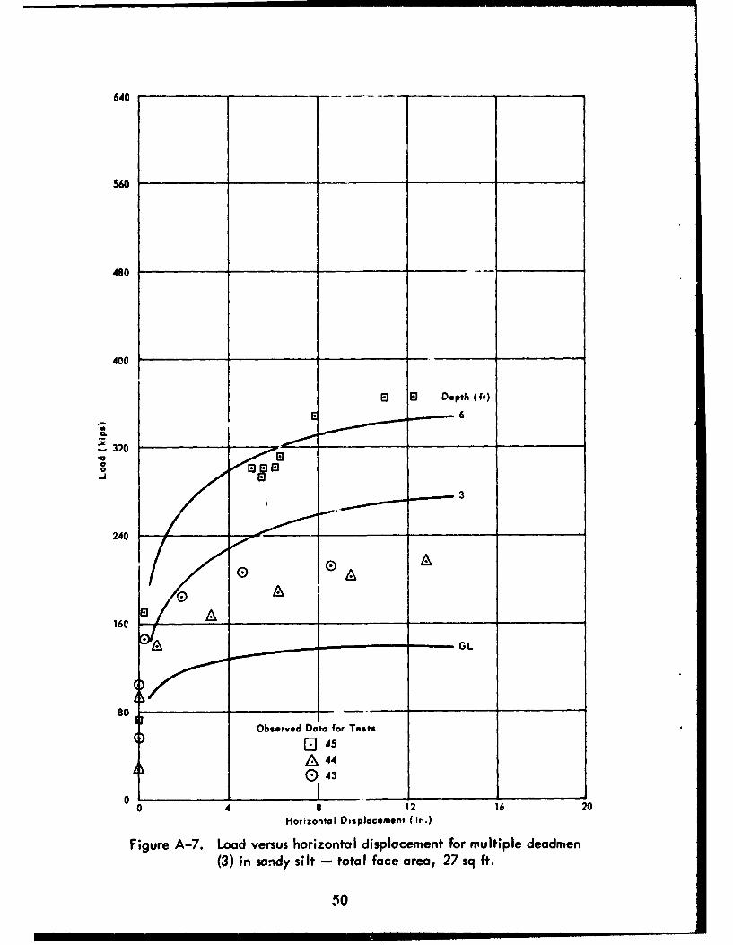
Figure A-7. Load versus horizontal displacement for multiple deadmen(3) in sandy silt - total face area, 27 sq ft.

50

640__ _

560

40

400Observed Data for Tests

47

C 46

-320 -_____

240

Depth (ft)

160

3

00 4 8 12 16 20

Horizontal Displacement (in.)

Figure A-8. Load versus horizontal displacement for single deadmenin silty sand - face area, 13.5 sq ft.

51

640

560

480

Observed Data for Tests

951

500 49

400Depth (ft)

320 r

240 3v

00 4 8 12 16 20

Horizontal Displacement (in.)

Figure A-9. Load versus horizontal displacement for single deadenin silIty sand -- face area, 27 sq ft.

52

640

560 Depth (ft)

6

480 ;J

13

is 3,

A A.A

t 320

-JG

Vol

530 52

0 4 8 12 16 20

Hotixontal Displacement (in.)

Figure A-10. Load versus horizontal displacement for single deadmenin siltyband - face area, 54 q ft.

53

640

560

480

400Observed Data for Tests

El 52A 49

( 46.LL

-320a

.J

240Face Area (Sq ft)

160 Val__

80 i, ,

.............. 13.5

0-0 4 8 12 16 20

Horizontal Displacement (in.)

Figure A-i 1. Load versus horizontal displacement for single deadmenin silty sand - depth, GL.

54

560

Observed Data for Tests

(D53A 50

400 _ _ _ _ __

Face Areab (sq ft)

54

C- A

240 27-

160P ____

00 4 8 12 16 20

Horizontal Displacemtent (in.)

Figoire A-12. Load versus horizontal displacement for single deadmenin silty sand - depth, 3 ft.

55

640

560 El .. Face Area (sq ft)

1 El • 54

480 E o '

400

27

CL,

240

8o ) -

10 w__w

[]48

5 4

0 4 8 12 16 20

Horizontal Displacement (in.)

Figure A-13. Load versus horizontal displacement for single deadmenin silty sand - depth, 6 ft.

56

640

560

480

Observed Date for Tests

E)57A 560 s5

400

Depth (ft)

.6

:320

3

240

160 A

0 4 I 12 16 20Horizontol DispIocemnt (in.)

Figure A-14. Load versus horizontal displacement for multiple deodmen(3) in silty sand - total face area, 27 sq ft.

57

640

560

This graph illustrates the curve fits for observeddata from tests in sand obtained using the equationpreviously Jetermined and described in Reference 2.

480

Observed Data for Tests

0 26A25Q24

400

Depth (ft)

4

- 320V

240

* ElEl El El E

160

• .... • GL

8 0 0 G 0 (

0 4 8 12 16 20Horizontal Displacement (in.)

Figure A-15. Load venus horizontal displacement for single deadmenin sand - face area, 72 sq ft.

58

Appendix B

MATHEMATICAL ANALYSIS

S. H. Brooks, Sc. D., CEIR, 1. W. Anders and W. L. Wiscoxson, NCEL

The data from the 57 tests of prototype anchors and 94 tests of model anchorswere analyzed. The data consisted of sets of ordered pairs of numbers (P, d) repre-senting the holding power of each anchor at given displacements. In general, thefollowing properties appear to exist between the holding power and the displacement:

1. At small values of the holding power, the holding power is linearly relatedto the anchor displacement.

2. As the holding power is increased, less additional holding power isassociated with a given further displacement.

3. There is a maximum holding power.

A simple relation consistent with these properties is

AP = R(m - P)Ad (;-I)

where d = horizontal displacement of deadman

Ad = an increment of displacement

P = force, or deadman holding capacity, required to achieve thatdisplacement

AP = an increment of deadmon holding capacity

m = maximum holding capacity which a deadman can attain withoutcontinuous displacement

R = rate constant which indicates how a change in holding capacity ,AP)is related to a small change in displacement (Ad)

When the force P is small, the above formula becomes P = R(m)Ad so thatproperty 1 above is satisfied. Properties 2 and 3 can be confirmed by noting that asP increases, (m - P) and therefore AP decreases for fixed Ad, and that when P = m,AP is zero. This relation expressed as a differential equation is

P'(d) = R (m - P) (B-2)

A solution to this equation is

P = m[1 - eR(d - b) (8-3)

59

where b is the displacement at which the force required is zero. This may also be

expressed as

P m(I - e-Rd) + ke-Rd (B-4)

where k is the force at the zero point on the displacement scale. A representation ofthis equation is shown in Figure B-1.

P

m

Ob 0,0

Figure B-1. Graph of Equation B-4.

Fitting the Curve to Equation B-4:

Let Am, Ak, and AR be identically equal to their differentials. An incrementof force may then be approximated by a function of m, k, and R as

AP = •Am + Ak + - AR (B-5)

Assume the parameters are some arbitrary value, say m0 , k0 , R0 . From Equations B-4and B-5,

+ (P - m 0P= P0 + (m-m0)- mo, k0, +0 m0, k(y R0

+ (R - R0) ,Rmop kor R0

60

* 0d -Red -R.d-- 0 -e + koe + (m mo0 )( - )

-Rod -Rod

+ (c - k0)e + (mn0 - k0 )(R - Ro)de 0 (B-6)

Equation B-6 reduces to

-Rod -Rod d-R~d

P i m(1 - e ) + ke 0 + (m0 - k0 )(R - RO)de (B-7)

-RodLeTting

U = 1 - e

= -Rod

(B-8)-RodW=de 0

Q (m- k0 -R 0-

there results P mU + kV + QW

The statistical model to be fitted is then

P. = U.m + V.k + W.Q + . (B-9)I I I I I

-Rd -Rod

where Ui = 1 - e , Vie 0 , Wi = diVi, Pi and do are the set of observations,and ei is the deviation of the ith observation from the fitted curve. Rearranging,squaring, then summing over the n observations ir Equation B-9 results in

n n1

C' 2 (Pi2 U'm - V'k - W'Q)2 (B-10)

1=1 i 61

61

To minimize the sum of squares of the errors, differentiate partially withrespect to each parameter and equate each of the results to zero. This leads tothe three simultaneous equations:

o U.'+ k U.V. + Q0 U.W. = 7U.P.

M7u.U. + k V. + QZ .w. v 7 .. (i i i i i 7 ipi (B-1 1)

m--UW.i+ kI'V.W. + Q!7Wi2 = P

Let = 7u 2 C 2 '7 uiV.. C13 =Y'Tuiw.. C1 = UP1

U 2 , = 2 V 2, C1 3 =7ViW C2j .7VP

(B-12)

C = 7W.2,c 3 7w .

C.. P.I2

Also let A CC - C132

B = C 12 C3 3 - 13C23

C = C2 2 C3 3 - C2 32 (B-13)

E C= I Cj33 - 3jC13

F =C 2 iC3 - C3 iC2 3

62

Using the symbols of Equations B-12 and B-13, it car. be shown that the solutions toEquation B-1O for m, k, and Q are

EC - FBm = (B-14)

AC -B 2

k F - mB (B-15)C

= C3 - mC 13 - kC23

C33

The analytical expression for the variance of the deviations of the observationsfrom the fitted curve is

11 c -m *j- kC2 - QC 3 .

C.-m= _H___K2 __ (B-17)n -3

which should, upon convergence, be nearly the some as

n n

7 [P' 2 = I Vn 3 [Pi(obs) " i(fit) n - 3 'Pi(obs)

-Rd. -Rd.i 2- m(! - e - ke'] (E-18)

From Equation B-8,Q

R 0 +in -k 0 (B-19)

Iterate, letting R0 = R, k0 = k, and m0 = m, until

I-_ < , -< k R <6 (B-20)in0 1 01 R0

where 6 is some pi'edetermined small number. (The minimum value for 6 wasdetermined as 1.0 x 10-5 for the IBM 1620 floating point subroutines. Smaller valuescaused endless wandering or resulted in oscillatory values for the parameters.)

63

Compared to k and R, m was found to be relatively stable; i.e., the valueobtained for m on the first iteration was nearly the same as the final value. Therefore,let m = m0 in Equation B-19. This changes Eqaution B-6 tu

P P + (R - RO)0o + (k - k 3) k ko r Ro0 k Ro

-Rod -Rod -Rod

m(1 - e ) + ke + (m - Ro 0 de (B-2 1)

Since the data is in an ascending _. ler, let

k0 =P 1 (9-22)

A procedure to construct the initial quess of R is

,:) Assume

m = P (B-23)n

(b) Choose some value P. such that

S>2 I(P 1 + P (B-24)

(c) From Equafion B-4,

I -Rod.T (P+Pn ) Pn (Pn - PI)e (8-25)

1

or R > -In2 (8-26)u d.

(d) Therefore, choose

(B-27)

I IId.

64

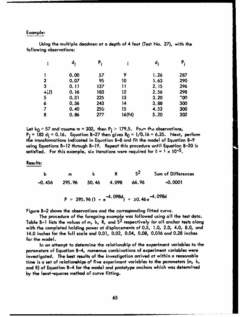
Example:

Using the multiple deadmen at a depth of 4 feet (Test No. 27), with thefollowing observations:

di Pi i d. Pi

1 0.00 57 9 1.26 2872 0.07 95 10 1.63 2903 0.11 137 11 2.15 2964(J) 0.16 183 12 2.56 2985 0.31 225 13 3.20 -0O6 0.36 243 14 3.88 3007 0.40 250 15 4.52 3008 0.86 277 16(N) 5.20 302

Let k0 = 57 and emsaume m = 302, then P- > 179.5. Frtm th. observations,P1 = 183 d- = 0.16. Equation B-27 then gives R0 = 1/0.16 = 6.25. Next, performthe transformations indicated in Equation B-8 and fit the model of Equation B-9using Equations B-12 through B-19. Repeat this procedure until Equation B-20 issatisfied. For this example, six iterations were required for 6 = 1 x -5

Results:

b m k R S2 Sum of Differences

-0.456 295.96 50.46 4.098 66.96 -0.0001

P = 295.96(1 0- e-4.098d) -* 0. 46 e -4.098d

Figure B-2 shows the observations and the corresponding fitted curve.The procedure of the foregoing example was followed using all the test data.

Table B-1 lists the values of m, k, R, and S2 respectively for all anchor tests alongwith the completed holding power at displacements of 0.5, 1.0, 2.0, 4.0, 8.0, and14.0 inches for the full scale and 0.01, 0.02, 0.04, 0.08, 0.016 and 0.28 inchesfor the model.

In an attempt to determine the relationship of the experiment variables to theparameters of Equation B-4, numerous combinations of experiment variables wereinvestigated. The best results of the investigation arrived at within a reasonabletime is a set of relationships o. five experiment variables to the parameters (m, k,and R) of Equation B-4 for the model and prototype anchors which was determ;nedby the least-squares method of curve fitting.

65

300 0 0

0 0 P 295.96(1 - -4.098d) + 50.46 e-4.098d

250

200

150 -

100

5o -4--k =50.46

0 1.0 2.0 3.0 4.0 5.0 6.0

b = -0.0456 d

Figure B-2. Graph of example for the multiple deadmen at adepth of 4 ft (Test No. 27).

These relationships are as follows:

m A IXIX2 + A 2 3 3X1 2 X4 + A4X1 + A5 (X4 + X5 ) + A6

k =B 1 X1 X2 + B2 X3 + B3 X 1 X 2 X 4 + B4 X1 + B5 (X 4 + X5 ) + B6

R C CXIX 2 + C2 X3 + C3 X1 X2 X4 + C4 X 1 + C5 (X4 + X5 ) + C6

where X1 = number of anchors

X 2 = area of the anchors

X 3 = cohesion of the soil

66

X4 = Depth to the top of the anchor

X5 = Height of the anchor

For the prototype:

A Values B Values C Values

A, = 1.444 BI = 0.882 CI = -0.006

A2 = 32.628 B2 = -0.920 C2 = -0.119

A3 = 1.077 3 = 0.717 C3 = 0.001

A4= 12.306 B4 = 18.419 C4 = 0.012A5 =.926 5= 4.216 C= 0.082

A6 = 59.564 B6 = -29.418 C6 = 1.367

and for the model:

A Values B Values C Values

A, = 0.152 3 = 0.044 C1 = 0.391

A2 = 40.515 B2 = 11.337 C2 = 4.213

A3 = 0.516 B 03 = 0.197 C3 = 0.043

A4 = 3.033 4 = 0.033 C4 = 0.729

A5 = 3.510 5 = 2.C C5 = 3.060

A6 = 55.883 B6 = 20.728 C6 = 56.321

Statistically, there is a high correlation between observed data and calculatedresults using the derived relationships in Equation B-4. However, for certain combi-nations of the variables, inexplicable inconsistencies occur. Thus for engineeringdesign purposes, application of Equation B-4 with the listed coefficients would behazardous and impractical.

67

Table B-I. Values of m, R, k, and S2 , and Holding Powers atDifferent Displacements for all Tests

Full-Scale Factors P(kips) for Displacement (in.) of

Test R k S2 0.5 1.0 2.0 4.0 8.0 14.0

1 8.20 1.09 5.30 0.0041 6.52 7.23 7.87 8.16 8.20 8.202 12.21 0.96 9.14 0.0036 10.32 11.04 11.76 12.14 12.21 12.213 24.22 1.46 15.32 0.0351 19.94 22.16 23.74 24.19 24.22 24.224 32.00 0.65 18.49 0.1560 22.25 24.96 28.34 31.00 31.92 31.995 46.15 0.59 20.35 0.0431 26.99 31.92 38.31 43.77 45.93 46.156 75.07 0.62 39.41 0.0242 49.00 56.02 64.89 72.16 74.83 75.077 150.23 0.33 103.34 0.6475 110.54 116.63 126.16 137.87 146.97 149.798 19.48 0.95 8.25 0.0014 12.51 15.16 17.82 19.23 19.47 19.489 27.00 0.67 12.55 0.0776 16.67 19.62 23.23 26.02 26.93 27.00

10 35.94 0.76 21.31 0.0493 25.96 29.13 32.77 35.26 35.91 35.9411 41.87 1.05 22.12 0.1908 30.20 34.98 39.47 41.58 41.87 41.8712 79.25 0.49 54.39 0.0534 59.87 64.14 70.07 75.86 78.79 79.2313 154.62 0.32 111.97 0.6348 118.35 123.77 132.31 142.95 151.43 154.1714 173.11 0.33 113.09 0.8130 122.35 130.19 142.42 157.42 169.01 172.5615 32.07 1.14 15.99 0.0442 23.01 26.97 30.45 31.90 32.07 32.0716 40.49 1.09 25.78 0.1554 31.98 35.56 38.84 40.31 40.49 40.4917 73.26 1.02 49.53 0.0429 59.08 64.78 70.23 72.87 73.25 73.2618 73.26 1.02 49.53 0.0429 59.08 64.78 70.23 72.87 73.25 73.2619 81.81 0.78 58.88 0.4669 66.34 71.37 77.06 80.82 81.76 81.81

20 148.44 0.57 103.90 1.6965 115.00 123.33 134.28 143.94 147.99 148.4321 259.40 0.43 182.77 4.2583 197.74 209.78 227.27 245.93 257.03 259.2322 63.50 0.66 30.85 0.1697 40.14 46.78 54.94 61.26 63.35 63.5023 167.95 0.38 85.59 0.4609 100.16 112.16 130.15 150.60 164.30 167.6024 84.65 0.63 48.41 0.3183 58.25 65.42 74.45 81.78 84.42 84.6425 222.54 0.46 124.11 3.4268 144.42 160.54 183.48 207.04 220.10 222.3926 373.46 0.46 272.62 3.2026 293.47 310.01 333.54 357.66 370.99 373.3127 304.93 0.73 255.23 1.0971 270.48 281.05 293.45 302.28 304.79 304.9328 93.36 0.82 63.27 0.5960 73.40 80.12 87.54 92.23 93.32 93.3629 232.61 0.67 183.19 4.2390 197.37 207.47 219.83 229.30 232.39 232.6130 322.09 0.66 277.84 0.7653 290.34 299.31 310.36 318.98 321.88 322.0931 108.63 0.63 83.41 0.4673 90.30 95.31 101.59 106.67 108.48 108.6332 242.48 0.52 200.23 1.7820 210.01 217.54 227.75 237.35 241.86 242.4633 328.09 0.57 267.69 1.1791 282.70 293.98 308.82 321.94 327.46 328.0734 74.72 0.44 13.93 0.5620 26.11 35.84 49.86 64.55 73.02 74.6035 122.62 0.23 39.61 0.9711 48.95 57.24 71.12 90.67 110.32 119.6836 171.99 0.22 73.36 5.8523 83.89 93.29 109.19 132.01 155.78 167.8137 131.35 0.42 32.44 1.5193 51.29 66.55 88.90 113.14 128.00 131.09

38 283.02 0.19 91.11 3.5559 109.17 125.53 153.78 195.98 243.54 270.9639 347.76 0.22 166.67 1.3753 186.28 203.77 233.27 275.38 318.83 340.4540 201.38 0.45 77.77 2.8938 102.75 ;22.6a 15i.27 181.07 198.04 201.1641 399.44 0.33 157.57 32.937 194.96 226.57 275.89 336.33 382.98 397.2542 568.08 0.23 300.71 39.681 329.81 355.74 399.45 461.73 525.78 557.4743 135.48 0.55 79.61 2.0553 93.09 103.32 116.97 129.34 134.80 135.4544 273.43 0.29 127.96 27.358 147.87 165.06 192.70 228.63 259.63 271.0745 345.50 0.34 174.66 43.155 201.68 224.43 259.70 302.41 334.63 344.1246 67.09 0.34 16.28 1.0350 24.34 31.12 41.62 54.33 63.88 66.6847 103.71 0.33 40.21 1.9878 49.99 58.27 71.19 87.05 99.34 103.1348 164.35 0.47 82.82 0.1373 100.14 113.77 132.98 152.28 162.56 164.2549 147.24 0.58 65.83 0.8009 86.58 102.04 122.14 139.50 146.50 147.2150 239.30 0.39 12'.63 10.978 142.48 159.64 185.37 214.58 234.10 238.8051 359.62 0.35 207.02 8.9149 231.94 252.80 284.84 322.98 350.82 358.5952 207.06 0.75 89.67 17.397 126.40 151.63 180.89 201.23 206.77 207.0653 349.77 0.37 197.99 56.362 224.11 245.74 278.46 316.27 342.38 349.0154 543.44 0.29 299.21 21.899 332.54 361.33 407.64 467.93 520.10 539.4355 127.05 0.82 41.42 0.8247 70.26 89.39 110.49 123.85 126.93 127.0556 270.29 0.26 86.82 11.283 109.31 129.04 161.55 205.84 247.65 265.5857 334.48 0.30 164.92 21.571 189.20 210.01 243.10 285.24 320.18 332.24

68

Table B-I. Values of m, R, k, and S2 , and Holding Powers atDifferent Displacements for all Tests (Contd)

Factors P(Ib) for Displacement (in.) of

Too i R k S2 0.01 0.02 0.04 0.08 0.16 0.28

1 9.51 33.22 3.09 0.0351 4.90 6.21 7.81 9.06 9.48 9.512 12.77 66.81 3.27 0.0849 7.90 10.28 12.12 12.73 12.77 12.773 17.20 48.61 6.91 0.0648 10.87 13.30 15.72 16.99 17.19 17.204 19.56 50.78 8.88 0.1587 13.13 15.69 18.16 19.38 19.56 19.565 25.02 42.26 13.80 0.2524 17.67 20.20 22.95 24.63 25.00 25.026 41.74 18.92 18.25 0.2627 22.30 25.65 30.72 36.57 40.60 41.627 42.80 10.68 26.27 0.9514 27.95 29.45 32.02 35.77 39.81 41.978 15.51 31.22 4.68 0.1392 7.58 9.71 12.41 14.62 15.44 15.519 19.36 26.39 7.32 0.0551 10.11 12.26 15.17 17.90 19.18 19.35

10 23.14 34.50 12.22 0.0206 15.41 17.67 20.40 22.45 23.10 23.1411 26.04 50.78 14.45 0.0918 19.07 21.85 24.52 25.85 26.04 26.0412 31.35 25.73 20.60 0.0210 23.04 24.93 27.51 29.98 31.17 31.3413 44.85 10.21 29.85 0.1027 31.31 32.63 34.88 38.23 41.93 43.9914 41.82 20.07 24.41 0.4019 27.57 30.17 34.02 38.33 41.12 41.7615 18.06 24.65 7.98 0.2551 10.18 11.91 14.30 16.66 17.87 18.0516 24.26 26.68 8.63 0.1651 12.29 15.09 18.88 22.41 24.04 24.2517 31.38 27.65 10.78 0.1938 15.76 19.53 24.56 29.12 31.13 31.3718 31.38 27.65 10.78 0.1938 15.76 19.53 24.56 29.12 31.13 31.3719 35.54 25.78 14.92 0.1817 19.61 23.23 28.19 32.92 35.20 35.5220 41.60 18.50 22.31 0.3542 25.57 28.28 32.40 37.21 40.60 41.4921 54.65 26.81 32.48 0.1325 37.69 41.68 47.06 52.05 54.35 54.6422 25.06 18.47 6.56 0.0480 9.68 12.28 16.22 20.84 24.10 24.9523 43.40 19.53 14.90 0.7277 19.95 24.11 30.35 37.43 42.15 43.2824 40.37 23.04 13.85 0.4115 19.31 23.64 29.82 36.17 39.70 40.3325 57.17 12.93 20.27 0.2661 24.75 28.68 35.18 44.06 52.51 56.1826 66.84 15.18 27.77 0.3220 33.28 38.01 45.56 55.25 63.40 66.2927 58.48 15.74 29.83 0.1103 34.01 37.57 43.22 50.36 56.18 58.1428 35.88 21.58 13.95 0.0852 18.21 21.64 26.63 31.98 35.19 35.8329 51.43 17.70 23.39 0.2302 27.94 31.76 37.62 44.63 49.78 51.2330 76.89 15.05 38.35 0.2672 43.74 48.37 55.79 65.33 73.42 76.3231 36.52 31.11 14.34 0.2422 20.27 24.61 30.13 34.68 36.36 36.5132 61.22 20.37 27.98 0.1747 34.11 39.10 46.51 54.71 59.94 61.1133 76.33 19.41 38.53 0.1361 45.20 50.70 58.94 68.33 74.64 76.1634 49.17 27.82 12.60 0.7338 21.48 28.21 37.15 45.22 48.75 49.1635 96.31U 13.71 33.60 4.7741 41.63 48.64 60.07 75.36 89.31 94.9536 142.51 18.19 44.89 0.1233 61.13 74.66 95.35 119.73 137.19 141.9137 77.19 17.42 28.41 0.0624 36.21 42.76 52.90 65.09 74.19 76.8238 158.11 9.43 51.78 1.5069 61.36 70.07 85.22 108.14 134.63 150.5539 235.33 9.96 95.81 4.0145 109.04 121.02 141.68 172.46 207.00 226.7640 118.76 12.62 31.74 1.4984 42.06 51.16 66.24 87.07 107.22 116.2241 218.85 9.24 76.90 0.7904 89.44 100.87 120.80 151.12 186.53 208.2042 369.31 9.13 147.43 3.5054 166.80 184.47 215.32 262.44 317.84 352.1043 107.73 14.02 20.66 1.7544 32.05 41.96 58.05 79.39 98.50 106.0244 201.65 9.90 47.43 10.212 61.98 75.16 97.90 131.85 170.06 192.0345 246.29 13.30 90.33 2.1528 109.76 126.77 154.69 192.49 227.73 242.5346 43.88 31.48 7.57 1.0444 17.38 24.54 33.58 40.96 43.65 43.8847 76.25 19.09 22.98 0.3109 32.24 39.89 51.43 64.68 73.74 75.9948 120.03 19.V7 48.78 0.4833 61.63 72.16 87.86 105.50 117.07 119.7649 70.59 14.49 16.57 0.8299 23.86 30.17 40.34 53.65 65.28 69.6650 129.67 14.01 36.73 1.6614 48.88 59.45 76.61 99.38 119.80 127.8451 195.57 18.18 63.54 22.652 85.50 103.80 131.78 164.75 188.38 194.7652 105.79 11.40 17.71 0.1764 27.20 35.66 49.96 70.41 91.57 102.1753 200.62 8.61 72.94 5.3403 83.48 93.15 110.16 136.53 168.45 189.1854 356.22 6.81 113.51 2.8686 129.51 144.46 171.46 215.57 274.71 320.2655 86.58 16.17 19.25 0.7973 29.30 37.85 51.32 68.12 81.52 85.8656 153.72 14.35 46.91 1.4730 61.20 73.57 93.57 119.85 142.98 151.8057 237.08 13.14 72.28 0.3631 92.58 110.37 139.66 179.49 216.95 232.92

69

Table B-I. Values of m, R, k, and S2, and Holding Powers atDifferent Displacements for all Tests (Contd)

Mdel Factors P(Ib) for Displacement (in.) of

Test m R k S2 0.01 0.02 0.04 0.08 0.16 0.28

58 34.56 19.72 9.86 0.4285 14.28 17.91 23.34 29.46 33.51 34.4659 47.94 19.31 24.31 0.5988 28.46 31.88 37.03 42.90 46.86 47.8360 60.22 15.97 33.60 0.0380 37.53 40.88 46.17 52.81 58.16 59.9261 39.39 11.10 10.90 0.3773 13.90 16.58 21.12 27.68 34.58 38.1262 34.03 11.59 8.13 0.6107 10.96 13.49 17.74 23.78 29.98 33.0263 45.83 12.34 13.54 0.1510 17.29 20.60 26.12 33.80 41.35 44.8164 51.9' 13.41 15.31 1.4431 19.91 23.93 30.51 39.40 47.64 51.0765 61.59 19.75 27.93 0.0845 33.96 38.91 46.31 54.66 60.16 61.4666 58.38 15.40 20.79 0.0488 26.16 30.76 38.08 47.42 55.18 57.8867 86.12 17.17 25.30 0.9314 34.90 42.98 55.52 70.73 82.22 85.6268 110.77 27.13 29.42 1.7164 48.75 63.49 83.29 101.49 109.71 110.7369 87.75 5.24 12.47 7.3392 16.32 19.97 26.73 38.28 55.24 70.4370 121.51 4.84 25.80 0.2212 30.33 34.64 42.66 56.55 77.42 96.8671 131.50 5.57 26.86 1.2134 32.54 37.91 47.79 64.53 88.64 109.5672 139.62 4.87 23.71 6.3090 29.22 34.47 4.23 61.12 86.45 109.9873 187.93 4.72 40.70 1.6325 47.49 53.97 66.04 87.02 118.77 148.6874 118.86 7.27 32.60 0.6620 38.65 44.28 54.37 70.65 91.92 107.6075 173.56 7.31 62.70 0.5019 70.53 77.80 90.84 111.83 139.19 159.2876 122.67 9.73 40.56 0.1432 48.18 55.09 67.05 84.99 105.38 117.2977 211.37 8.44 67.65 0.2058 79.30 90.00 108.87 138.26 174.18 197.8778 304.08 9.21 122.31 8.6656 138.31 152.90 178.35 217.11 262.47 290.3179 143.26 12.04 59.93 0.7214 69.39 77.77 91.79 111.47 131.13 140.4080 208.65 9.87 87.01 0.6949 98.45 108.81 126.70 153.44 183.59 200.9881 79.02 9.45 12.38 0.9275 18.39 23.86 33.36 47.73 64.33 74.2982 93.43 8.22 22.30 12.076 27.91 33.08 42.23 56.58 74.34 86.3183 128.51 7.69 34.01 1.0820 41.01 47.49 59.05 77.45 "C i2 117.5584 116.53 8.11 27.20 0.5915 34.16 40.57 51.95 69.84 ý2.13 107.3185 175.61 6.20 59.06 5.0768 66.06 72.65 84.66 104.64 132.39 155.0786 82.87 10.98 8.21 0.6684 15.98 22.94 34.76 51.87 70.00 79.4387 164.22 8.28 43.60 3.4327 53.19 62.02 77.63 102.06 132.19 152.3788 100.54 13.00 29.48 0.3493 38.14 45.75 58.30 75.43 91.67 98.6789 167.01 10.74 58.59 0.4506 69.63 79.55 96.46 121.10 147.57 161.6590 287.87 8.01 108.80 0.2889 122.59 135.32 157.91 193.56 238.20 268.8891 123.22 13.62 46.54 0.7890 56.31 64.84 78.77 97.45 114.56 121.5492 183.24 10.59 73.74 0.7469 84.74 94.64 111.55 136.31 163.13 177.6093 146.22 11.01 27.38 7.7127 39.78 50.88 69.73 96.98 125.82 140.7894 119.35 8.02 12.38 0.4729 20.63 28.24 41.75 63.06 89.73 108.05

70

REFERENCES

1. U. S. Naval Civil Engineering Laboratory. Technical Memorandum M-121:Tests of concrete deadman anchorages in sand, by J. E. Smith. Port Hueneme,Calif., Feb. 1957.

2;.. Technical Report R-199: Deadman anchorages in sand, by J. E. Smith.Port Hueneme, Calif., July 1962.

3. G. P. Tschetobarioff. Soil mechanics, foundations, and earth structures.New York, McGraw-Hill, 1951.

71

DISTRIBUTION LIST

CHIEF. BUREAU OF YARDS AND DOCKS (CODE 42)

COMMANDER. NAVAL CONSTRUCTION BATTALIONS. U. So ATLANTIC FLEET, DAVISVILLE,RHODE ISLAND 02854

COMMANDER, NAVAL CONSTRUCTION BATTALIONS* PACIFIC. FPO SAN FRANCISCO 96610

COMMANDING OFFICER9 MOBILE CONSTRUCTION BATTALION NO. 6, FPO NEW YORK 09501

COMMANDING OFFICER, MOBILE CONSTRUCTION BATTALION NO. 7, FPO NEW YORK 09501

COMMANDING OFFICER, MOBILE CONSTRUCTION BATTALION NO. 89 FPO SAN FRANCISCO96601

COMMANDING OFFICER. AMPHIBIOUS CONSTRUCTION BATTALION 19 SAN DIEGO, CALIF*92155

COMMANDING OFFICER. AMPHIBIOUS CONSTRUCTION BATTALION 2. FPO NEW YORK 09501

OFFICER IN CHARGE* WESTERN PACIFIC DETACHMENT, AMPHIBIOUS CONSTRUCTIONBATTALION 1, FPO SAN FRANCISCO 96662

CHIEF, BUREAU OF SUPPLIES AND ACCOUNTS, NAVY DEPARTMENT, WASHINGTON, Do Ce20360

COMMANDING OFFICER, OFFICE OF NAVAL RESEARCH, BRANCH OFFICE. ATTN PATENTDEPARTMENT* 1030 EAST GREEN STREET, PASADENA, CALIF. 91101

COMMANDING OFFICER, ATTN PUBLIC WORKS OFFICER, NAVAL STATION. KEY WEST.FLA* 33040

COMMANDING OFFICER, ATTN PUBLIC WORKS OFFICER, NAVAL STATION. LONG BEACH,CALIF 90802

COMMANDING OFFICER, ATTN PUBLIC WORKS OFFICER, NAVAL STATION, SAN DIEGO.CALIF. 92136

COMMANDING OFFICER. ATTN PUBLIC WORKS OFFICER, U. So NAVAL STATION, FPO NEWYORK 09585

COMMANDING OFFICER. ATTN PUBLIC WORKS OFFICER, U. So NAVAL COMMUNICATIONSTATION. ROUGH AND READY ISLAND. STOCKTON, CALIF. 95203

COMMANDING OFFICER. U. So NAVAL COMMUNICATION STATION, FPO SAN FRANCISCO96680

COMMANDER, FLEET ACTIVITIES, ATTN PUBLIC WORKS OFFICER, FPO SAN FRANCISCO96666

COMMANDING OFFICER, ATTN PUBLIC WORKS OFFICER. U. So NAVAL SUBMARINE BASE.NEW LONDON9 GROTON. CONN* 06342

COMMANDING OFFICER, NAVAL AMPHIBIOUS BASE, LITTLE CREEK. NORFOLK. VA. 23521

'COMMANDING OFFICER, ATTN PUBLIC WORKS OFFICER, NAVAL RECEIVING STATION,136 FLUSHING AVENUE, BROOKLYN* NEW YORK 11251

COMMANDING OFFICER. NAVAL STATION. ANNAPOLIS, MD* 21402

OFFICER IN CHARGE, NAVAL CONSTRUCTION TRAINING UNIT, NAVAL CONSTRUCTIONBATTALION CENTER, DAVISVILLE, Ro to 02854

UnclassifiedSecuuity Clameifcation

DSeadmtransIicto Ac ofag te, In y Vrofs Soilec m Mnediumsnoainms eenee *n0 vi eotI lsiidI4. OE5RIPATN0ATIVINTES (Cp.ooperaeiftw mts. REPORTi SEURTYCLSSFIA)O

Final; Sept 1962 - March 1965S. AUTHOR(S) (L.at name. firm# Room, Initial)

Smith, J. E.Stalcup, J. V.

G. REPORT DA TIE7aTOANOOFA0 7.o.irmsApril1 9%667

Ga. CONTRACT afR SRAN4T NO. 90. @RSIONATORIG REPORT NUMeaR(S)

66 PROJECT NO0. Y-F015-15-O1-01O TR-434

c. 9 . Z~m=PORT ma(S) (Any *Moe? nmammbe. lml may ba caesioed

10. A VA IL ASILITY/LIMITATION NOTICES

Distriobution of this document is unlimited.

11. SUPPLEMENTARY NOTES 12. SPONSORING MILITARY ACTIVITY

Copies available at the Clearinghouse BUDOCKS(CFSTI) $3. 00.

12. AUSTRACT

A test program was conducted to investigate deadman anchorage holding capacitiesunder applied horizontal loads. Deadmen fabricated of concrete and ranging in face areafrom 5 to 72 square feet were tested in depths of embedment from ground level to 7 feet.The deadmen were pulled both singly and in groups of three, in sand and in two soils withcohesive characteristics. The test program also included tests on i model scale.

The investigation disclosed that multiple anchors develop a higher holding capacityper net area than a single deodman with the same total face area. The increase in holdingcapacity ranging from 5 to 20% depends upon such factors as depth of embedment, the typeof soilI, and the spacing between deadmen. Under mast test conditions, up to a 30%increase in holding capacities was attained in cohesive soilIs as compared to sand, but 2 to3 times the horizontal displacement was required to achieve the maximum holding capacity.

D D Tt~ 1473 ojoi-ol-80 UnclassifiedSecurity Classification

UnclassifiedSecurity Classification

1I. LINK A LINK 8 LINK CKEY WORD$ ROLE WT ROLE WT ROLE WT

TestsAnalysisDeadmonAnchoragesAnchorsDeterminationHolding powersSoilsHorizontalLoads (forces)DesignGraphs (charts)

INSTRUCTIONSt. ORIGINATING ACTIVITY: Enter the name and address imposed by security classification, using standard statementsof the contractor. subcontractor, grantee, Department of De- such as:fense activity or other organization (corporate author) issuing (1) "Qualified requesters may obtain copies of thisthe report. report from DDC."2&. REPORT SECURETY CLASSIFICATION: Enter the over- (2) "Foreign announcement and dissemination of thisall security classification of the report. Indicate whether"Restricted Data" is included. Marking is to be in accord; report by DDC is not authorized."snce with appropriate scurity regulations. (3) "U. S. Government agencies may obtain copies of

this report directly from DDC. Other qualified DDC2b. GROUP, Automatic d:wngrading is specified in DOD Di- users shall request throughrective 5200. 10 and Armed Forces Industrial Manual. Enterthe group number. Also, when applicable, show that optional •"markings have been used for Group 3 and Group 4 as author- (4) "U. S. military agencies may obtain copies of this£zeldl. report directly from DDC. Other qualified users

3. REPORT TITLE: Enter the complete report title in all shall request throughcapital letters. Titles in all cases should be unclassified.If a meaningful title cannot be selected without classifica-tion. show title classification in all capitals in parenthesis (5) "All distribution of this report is conttolled. Qual-immediately following the title, ified DDC users shall request through

4. DESCRIPTIVE :ODTES: Af appropriate, enter the type of _"

report, e.g.. interim, progress, summary, annual, or final. If the report has been furnished to the Office of TechnicalGive the inclusive dates when a specific reporting period is Services, Department of Commerce, for sale to the public, indi-covered, cate this fact end entcr the price, if known.S. AUTHOR(SY. Enter t.e i-ame(s) of author(s) as shown on IL SUPPLEMENTARY NOTES: Use for additional explana-or in the report. Enter last name, first name, middle initial, tory notes.If military, show rank and branch of service. The name ofthe principal author is an ahsolute minimum requirement. 12. SPONSORING MILITARY ACTIVITY: Enter the name of

the departmental project office or laboratory sponsoring (pay.6. REPORT DATEL Enter the date of the report as day. inm for) the research and development. Include address.month, year or month, year. If more than one date appearson the report, use date of publication. 13. ABSTRACT: Enter an abstract giving a brief and factual

summary of the document Indicative of the report, even though7.. TOTAL NUMBER OF PAGES: The total page count it may also appear elsew..ere in the body of the technical re-should follow normal pagination procedures, i.e.. enter the port. If additional space is required, a continuation sheet shallnumber of pages containing information, be attached.7b. NUMBER OF REFERENCES Enter the total number of It is highly desirable that the abstract of classified reportsreferences cited in the re.,rt. be unclassified. Each paragraph of the abstract shall end withRa. CONTRACT OR GRANT NUMBER: If appropriate, enter an indication of the military security classification of the in-the applicable number of the contract or grant under which formation in the paragraph, represented as (TS). (S). (C). or (U)the report was written. There is no limitation on the length of the abstract. How-Sb, &8, & Sd. PROJECT NUMBER: Enter the appropriate ever, the suggested length is from 150 to 225 words.military department identification, such as project number,subproject number, system numbers, task number, etc. 14. KEY WORDS: Key words are technically meaningful terms

or short phrases that characterize a report and may he used as9a. ORIGINATOR'S REPORT NUMBER(S): Enter the offi- index entries for cataloging the report. Key words must becial report number by which the document will be identified selected so that no security classification is required. Identi-and controlled by the originating activity. This number must fiers, such as equipment model designation, trade name, militarybe unique to this report. project code name, geographic location, may be used as key9b. OTHER REPORT NUMBER(S): If the report has been words but will be followed by an indication of technical con-assigned any other report numbers (either by the orilinator text. The assignment of links, rules, and weights is optional.or by the sponsor), also enter this number(s).10. AVAILABILITY/LIMITATION NOTICES: Enter any lina-Rtations on further dissemination of the report, other than those

Unc lass i fiedSecurity Classification