defending an asset: a linear quadratic game approach

Defending an Asset: A Linear

Quadratic Game Approach

DONGXU LI

General Motors Company

JOSE B. CRUZ, JR.

The Ohio State University

Techniques based on pursuit-evasion (PE) games are often

applied in military operations of autonomous vehicles (AV) in

the presence of mobile targets. Recently with increasing use of

AVs, new scenarios emerge such as surveillance and persistent

area denial. Compared with PE games, the actual roles of the

pursuer and the evader have changed. In these emerging scenarios

the evader acts as an intruder striking at some asset; at the same

time the pursuer tries to destroy the intruder to protect the asset.

Due to the presence of an asset, the PE game model with two

sets of players (pursuers and evaders) is no longer adequate.

We call this new problem a game of defending an asset(s) (DA).

In this paper we study DA games under the framework of a

linear quadratic (LQ) formulation. Three different DA games are

addressed: 1) defending a stationary asset, 2) defending a moving

asset with an arbitrary trajectory, and 3) defending an escaping

asset. Equilibrium game strategies of the players are derived for

each case. A repetitive scheme is proposed for implementation of

the LQ strategies, and we demonstrate with simulations that the

LQ strategies based on the repetitive implementation can provide

good control guidance laws for DA games.

Manuscript received July 7, 2008; revised August 1, 2009; released

for publication November 22, 2009.

IEEE Log No. T-AES/47/2/940827.

Refereeing of this contribution was handled by V. Krishnamurthy.

Authors’ addresses: D. Li, General Motors Company, R&D, 30500

Mound Rd., Warren, MI 48090, E-mail: ([email protected]); J. B.

Cruz, Jr., Dept. of Electrical and Computer Engineering, The Ohio

State University, 205 Dreese Lab, 2015 Neil Ave., Columbus, OH

43202.

0018-9251/11/$26.00 c° 2011 IEEE

I. INTRODUCTION

The increasing use of autonomous vehicles (AV)

in modern military operations has recently led to

renewed interest in pursuit-evasion (PE) differential

games [1—4]. AVs deployed in a battlefield often

face intelligent opponents with mobility who can

usually make strategic decisions in response to AVs’

movements [5, 6]. A formulation based on one-sided

optimization is no longer adequate to model such AV

operations. As a tool for modeling decision-making

in conflict situations, game theory has advantages in

resolving the action-counter-action issues involved. PE

game models have been used in target tracking, strike

and object avoidance, etc.

In a typical PE game, one or a group of players

called pursuers go after another one or group of

players called evaders. To study the players’ optimal

strategies, the problem is usually formulated as a

zero-sum game in such a way that the pursuer(s)

tries to minimize a prescribed cost function while

the evader(s) tries to maximize the same function

[7, 8]. Dynamic programming (DP) is the only

general method for solving differential games. In

the literature a number of formal solutions regarding

optimal strategies in particular PE problems have been

achieved [7—10]. Due to the development of linear

quadratic (LQ) optimal control theory, a large portion

of the literature focuses on PE differential games with

a performance criterion in a quadratic form and linear

dynamics of the players [9, 11].

With the development of AV technologies and the

continued interest in AV applications, new scenarios

emerge such as surveillance and persistent area denial

[12]. A typical scenario usually involves an attacker,

who is about to attack some friendly assets. To protect

the assets, AVs are often tasked to destroy the attacker.

In this attack-defense problem, the attacker and the

AV are counterparts of the pursuer and the evader

in the sense that the AV wants to catch the attacker

while the attacker wants to avoid being caught. It

is also distinguished from PE games because the

players’ roles have changed. To chase or to escape

is no longer the mere task of the AV or the attacker.

Besides escaping, the attacker also needs to reach the

vicinity of the asset to attack. For the AV, it is crucial

that interception occurs before the attacker reaches the

asset. By nature this is a game played by the attacker

and the AV with involvement of an asset. We call it

the “game of defending an asset(s)” (DA). To the

authors’ knowledge, this is a first attempt to address

such a problem. As a first step, we focus on problems

where only three entities are present, i.e., an attacker,

an interceptor, and an asset.

Solution techniques that have been used for PE

games are not directly applicable to DA games. In

contrast to PE games, interception of the attacker here

is time sensitive and must occur before the potential

1026 IEEE TRANSACTIONS ON AEROSPACE AND ELECTRONIC SYSTEMS VOL. 47, NO. 2 APRIL 2011

attack. The term “capturability,” used in PE games

to indicate the pursuer’s capability of catching the

evader, is not adequate in a DA game when an

additional asset is taken into account. Taking an

arbitrarily long time in capturing is apparently not

acceptable. As we see in an example later, an optimal

pursuit strategy may not be a valid interception

strategy in a DA game.

The literature on DA games is very limited.

Only a special case has been discussed in [13]

and [7, p. 144], where the game was referred to

as the “game of defending a target.” In these two

references a problem in R2 was considered witha fixed target, and players have simple motion

dynamics. A geometric approach has been used to

determine optimal control strategies of the players.

Although the study in this paper is motivated by

AV applications, readers may find it relevant to the

areas of missile guidance and navigation [14]. In a

conventional navigation problem, control laws are

designed for an interceptor to track a moving target.

Proportional navigation guidance law and its variants

have been the most widely employed techniques for

nonmaneuvering target due to their simplicity and

ease of implementation [14]. However, they are not

adequate for DA games because of the involvement

of an extra asset and the fact that the attacker is

highly maneuverable. Another large class of relevant

guidance laws are designed under the framework of

optimal control theory, quite a large portion of which

are based on LQ optimal control theory [14].

For a DA game with an attacker, an interceptor,

and an asset, the main difficulty lies in the additional

terminal constraint of the game. In a (two-player) PE

game, the game terminates as long as the pursuer

is sufficiently close to the evader, while a DA

game may also end if the attacker and the asset

are sufficiently close. With this additional game

terminal constraint, meaningful game formulation

and theoretical development of solutions as well as

solution techniques become very difficult.

To satisfy the practical need for solving DA games

and avoid theoretical challenges, we approach DA

games with an approximate LQ formulation to make

use of the ample results in the LQ game theory. As

a practical approach, terminal penalty terms, also

referred to as soft constraints, are adopted to replace

the inherent hard constraints at the game terminal.

Three types of DA games are considered with respect

to the asset’s maneuverability, i.e., 1) the asset is

stationary; 2) the asset moves along an arbitrary

but known trajectory; and 3) the asset is escaping.

These cover all possible DA scenarios, and each has

a unique formulation and will be treated separately. To

apply the resulting LQ game strategies to “real-world”

DA problems, a practical algorithm based on repetitive

implementation is proposed. The performance of the

algorithm is demonstrated through simulations.

The paper is organized as follows. In Section II,

we introduce the DA problem and discuss difficulties

in problem formulation and solution techniques. In

Section III, a DA game is formulated with linear

dynamics and a quadratic objective based on soft

constraints. In Section IV, equilibrium strategies of

the players are derived for each of the three different

DA games regarding the asset’s maneuverability.

An implementation scheme is then introduced in

Section V to fill the gap between the LQ formulation

and “real-world” problems. In Section VI, we evaluate

the performance of the proposed strategies with

simulations of different DA games with simple

dynamics. Concluding remarks are provided in

Section VII.

II. THE PROBLEM OF DEFENDING ASSET

We first describe a general DA game and discuss

the theoretical difficulties. Consider an attacker, an

interceptor, and an asset in an nS-dimensional space

S μ RnS with nS 2 N. Let xa 2 Rna , xi 2 Rni , and xt 2 Rntbe the state variables of the attacker, the interceptor,

and the asset, respectively, with na,ni,nt ¸ nS. Thedynamics of the players are given in the following

differential equations in general terms:

_xa(t) = fa(xa(t),ua(t)) with xa(0) = xa0

_xi(t) = fi(xi(t),ui(t)) with xi(0) = xi0

_xt(t) = ft(xt(t),ut(t)) with xt(0) = xt0:

(1)

Here ua(t) 2Ua μ Rma , ui(t) 2Ui μ Rmi , and ut(t) 2Ut μ Rmt are the control inputs. Suppose that the firstnS elements of xa (or xi,xt) stand for the physical

position of the attacker (or interceptor, asset) in S.

In a DA game the asset (or attacker) is considered as

attacked (or intercepted) if it is within an " vicinity

of the attacker (or interceptor) for a small " > 0. Now

we define a projection operator P :Rna 7! S for the

attacker as

P(xa) = [xa1, : : : ,xanS ]T 2 S: (2)

That is P(xa) returns the attacker’s position in S.

A similar operator can also be defined for both the

interceptor and the asset, and for simplicity, we use

the same notation P. Given some " > 0, we define the

sets ¤1 and ¤2 as

¤1 = f(xi,xa,xt) 2 Rni £Rna £Rnt j kP(xa)¡P(xt)k · "g(3)

¤2 = f(xi,xa,xt) 2 ¤c1 j kP(xi)¡P(xa)k · "gwhere ¤c1 is the complementary set of ¤1; k ¢ k is thestandard Euclidean norm. Here ¤1 denotes the set of

the game states where the attacker has successfully

reached the vicinity of the asset to perform attacks;

whereas ¤2 stands for the states where the attacker

has been intercepted before it reaches the asset. Note

that in mathematical terms, attack and interception are

LI & CRUZ, JR.: DEFENDING AN ASSET: A LINEAR QUADRATIC GAME APPROACH 1027

abstracted to be the distances between the relevant

players. In general the value of " for attack and

interception may be different. Let ¤= ¤1 [¤2. Clearlythe set ¤ defines the terminal set of a DA game,

i.e., the game terminates at time T, T =minft > 0 j(xi(t),xa(t),xt(t)) 2 ¤g. In other words the gameterminates when either attack or interception occurs.

Here T is regarded as the terminal time of the game.

With the notations introduced above, a DA game

problem can be described as follows:

Given the initial states xa 2Rna , xi 2Rni , andxt 2Rnt , the intercepter (or with the asset in case ofa manoeuvrable asset) needs to find a proper control

input ui(t) (or with ut(t)) as a function of time based

on its accessible information, such that the game ends

in ¤2, i.e., (xi(T),xa(T),xt(T)) 2 ¤2; while the attackertries to drive the state trajectory into ¤1 by choosing a

proper input ua(t).

Generally speaking the game described above is a

game of kind1 [8], for which an analytical solution

is usually derived by introducing an auxiliary cost

function as follows. Assume that the game ends in

¤ in a finite time, and then we can define

J =

½0 if (xa(T),xi(T),xt(T)) 2 ¤21 if (xa(T),xi(T),xt(T)) 2 ¤1:

In this way, the game is converted into a differential

game of degree. The value function V (if it exists) can

only take two values: V(xa,xi,xt) = 1 and V(xa,xi,xt)

= 0, which is not differentiable. Please note that the

description above is not a rigorous definition of

a DA game, where no information structure is

specified, so the type of solutions has not yet been

determined.

Rigorous study of a DA game and possible

solution techniques involves tremendous challenges.

Optimal strategies of the players can possibly

be derived only when it is known where the

game state ends given an initial state (xa,xi,xt).

However, knowledge of terminal states implicitly

requires the existence of a value function, i.e.,

V(xa,xi,xt) = 1 or V(xa,xi,xt) = 0, as defined above.

However, rigorous demonstration of the existence

of solutions is not yet available and far from trivial.

Even for a less complicated two-player PE game

[15], rigorous definition and treatment involve

many theoretical difficulties. In the literature

establishment of the existence of solutions usually

requires certain players’ information structures

(such as the nonanticipative strategy in [15]).

Lipschitz continuity of players’ dynamic equations

1When we speak of differential game of kind, we mean a game

with finitely many, usually two, outcomes; the counterpart is called

differential game of degree, which has a continuum of possible

payoffs. The latter is the concept mostly used in the field of

differential games.

and continuity of the value V are necessary, and

the viscosity solution of the Hamilton-Jacobi-Isaacs

equation is adopted [16]. These assumptions are not

satisfied in a DA game.

Another difficulty lies in solution development,

which is related to dynamic programming. Suppose

that a value V exists, and we define the sets

Sj = f(xa,xi,xt) 2 Rni £Rna £Rnt j V(xa,xi,xt) = jgwith j 2 f0,1g. Here the set S0 (or S1) contains all theinitial states from which the interceptor (or attacker)

can successfully force the game to end in ¤2 (or

¤1). Only with knowledge of Si may an optimalstrategy of the interceptor (or attacker) be derived.

However, a formal derivation of Si is very difficult.Compared to PE games, the dimension of the state

space increases dramatically with the additional asset.

The numerical method [17] based on a reachable set

calculation is applicable, but actual implementation

can be problematic because the time horizon can

be arbitrarily large, and the method suffers from

the exponential growth in the number of states.

In summary a general DA game is a very difficult

problem.

III. LINEAR QUADRATIC FORMULATION WITHSOFT CONSTRAINTS

Theoretical exploration of the challenges discussed

in the previous section is out of the scope of this

paper. To satisfy the practical needs in solving

DA games, we take a practical approach by using

the LQ game theory. As can be seen, most of the

difficulties in a DA game are related to the hard

constraints imposed on the game terminal. In an LQ

formulation, hard constraints are often approximated

by soft constraints with weighting parameters in

the optimal control and differential game literature

[9, 18]. The soft constraints mean that the penalty

terms are introduced in the objective function with

a fixed optimization horizon. By this approximation

a problem with a fixed horizon can be formulated.

The key is to choose a proper optimization horizon.

Following the idea we reformulate a DA problem

as an LQ game using soft constraints with a fixed

horizon.

Suppose that each player in the game has an

independent dynamics

_xa(t) = Aaxa(t) +B0aua(t) with xa(t0) = xa0

(4a)

_xi(t) = Aixi(t)+B0iui(t) with xi(t0) = xi0 (4b)

_xt(t) = Atxt(t)+B0tut(t) with xt(t0) = xt0: (4c)

Here xa(t) 2 Rna , xi(t) 2 Rni , and xt(t) 2 Rnt forna,ni,nt ¸ nS and t¸ t0; ua(t) 2Ua, ui(t) 2Ui andut(t) 2Ut are control inputs; Aa,Ai,At,B0a,B0i ,B0t are realmatrices with proper dimensions. For simplicity, we


write an aggregate dynamic equation as

_x(t) = Ax(t)+Baua(t) +Biui(t)+Btut(t) (5)

where

x=

264xaxixt

375 , A=

264Aa 0 0

0 Ai 0

0 0 At

375

Ba =

264B0a

0

0

375 , Bi =

264 0B0i0

375 and

Bt =

264 00B0t

375 :Here x 2 Rn with n= ni+ na+ nt. We assume thateach player can access the state x at any time t, and

feedback strategies are considered, i.e., °a : Rn£R 7!Ua, °i :Rn£R 7!Ui and °t : Rn£R 7!Ut for the

attacker, the interceptor, and the asset, respectively.

Namely, given x 2Rn and time 0· t < T, °a(x, t) 2Ua,°i(x, t) 2Ui, and °t(x, t) 2Ut. Denote by ¡a, ¡i, or ¡tthe set of admissible feedback strategies for each of

the players. In this paper, three different DA games

regarding the asset’s maneuverability are discussed,

and the asset’s strategy is only relevant in one case.

We consider the objective function of the

following form

J(°a,°i,°t;x0)

=

Z T

0

(ua(¿)Tua(¿) +¸ut(¿)

Tut(¿)¡ uTi (¿)ui(¿)

+wIakP(xa(¿))¡P(xt(¿ ))k2¡wIi kP(xi(¿ ))¡P(xa(¿ ))k2)d¿ +wakP(xa(T))¡P(xt(T))k2

¡wikP(xi(T))¡P(xa(T))k2: (6)

In (6), °a,°i,°t are the feedback strategies; ¸ 2f0,¡1g is a binary variable2; ua, ui, ut are the controlinputs associated with each player’s strategy; wa,

wi, wIa, and w

Ii > 0, which are the weighting scalars

corresponding to the relevant costs induced by the

distance between the attacker and the asset and that

between the interceptor and the attacker. Instead of

hard constraints imposed on the game terminal, soft

constraint (penalty) terms with a fixed time duration T

are used. In this formulation, T, wa, wi, wIa,w

Ii are the

design parameters.

The objective J can be written in a quadratic

form with respect to x, ua, ui, and ut. First kP(xa)¡P(xt)k2 = xTQax and kP(xi)¡P(xa)k2 = xTQixwith Qa and Qi specified as

2Here ¸=¡1 indicates that the game is played among all the threeplayers while ¸= 0 is associated with the case where the asset’s

control is not relevant.

Qa =2666664InS 0

0 0na¡nS

0nS£ni0

¡InS 0

0 0(na¡nS )£(nt¡nS )

0ni£na 0ni 0ni£nt¡InS 0

0 0(nt¡nS )£(na¡nS )

0nS£ni0

InS 0

0 0nt¡nS

3777775and

Qi =2666664InS

0

0 0na¡nS

¡InS 0

0 0(na¡nS )£(ni¡nS )

0nS£nt0

¡InS 0

0 0(ni¡nS )£(na¡nS )

InS0

0 0ni¡nS

0

0

0nt£na 0 0

3777775where 0p£q is the zero matrix of dimension p£ q; 0p(or Ip) is the p£p zero (or identity) matrix; 0 is azero matrix of a proper dimension. Then J in (6) isequivalent to

J =

Z T

0

(uTa ua+¸uTt ut¡uTi ui+ xT(¿)Qx(¿))dt

+ xT(T)Qfx(T) (7)

where matrix Q = Q(wIa,wIi ), and Qf = Q(wa,wi) with

function Q(¢, ¢) defined asQ(wa,wi) = waQ

a¡wiQi:This is a zero-sum game between the attacker and

the interceptor (or the interceptor with the asset).The attacker seeks a strategy °a 2 ¡a to minimize J ,while the intercepter (or along with the asset) triesto maximize J with °i 2 ¡i (or °t 2 ¡t). This can beviewed as a dual tracking problem where the attackerwants to track the asset but to avoid the inceptor, andat the same time, the interceptor tries to follow theattacker closely.By casting the DA problem into an LQ game,

we can circumvent the technical difficulties, andderivation of game strategies becomes possible. Underthe LQ game framework, existence of solutions isequivalent to the existence of the underlying Riccatiequation, which may be checked under certainconditions [8, 19].In what follows, we discuss solution techniques

for each of the three different DA games regarding themobility of the asset: a DA game with 1) a fixed asset,2) a moving asset following an arbitrary trajectory,and 3) an escaping asset.

IV. GAME SOLUTIONS FOR DA GAMES WITHDIFFERENT TYPES OF ASSETS

A. Review of LQ Game Theory

Let us first review the LQ game theory that willbe the major tool used in this paper. Consider a


game involving two players with the following linear

dynamics:

_x(t) = Ax(t) +B1u1(t) +B2u2(t): (8)

The objective function is

J =

Z T

0

(u1(¿ )Tu1(¿)¡ uT2 (¿)u2(¿) + xT(¿)Qx(¿))d¿

+ xT(T)Qfx(T): (9)

Suppose that both of the players have access to the

state variables, and state feedback strategies are of

interest. The following theorem specifies saddle-point

equilibrium strategies.

THEOREM 1 The game with the players’ dynamics

in (8) and the objective J in (9) admits a feedback

saddle-point solution given by u¤1(t) = °¤1(x(t), t) =

K¤1 (t)x(t), and u¤2(t) = °

¤2(x(t), t) =K

¤2 (t)x(t) with K

¤1 (t) =

¡BT1Z(t) and K¤2 (t) = BT2Z(t), where Z(t) is bounded,symmetric, and satisfies

_Z =¡ATZ ¡ZA¡Q+Z(B1BT1 ¡B2BT2 )Z with

Z(T) =Qf: (10)

Readers are referred to [8] and [20] for a detailed

proof.

Theorem 1 provides solutions to a two-player

zero-sum LQ game. The implicit assumption here

is that a bounded solution for (10) exists over the

time horizon [0,T]. This nonlinear matrix differential

equation is called a Riccati equation. In the control

literature it is often required that matrices Q and Qfare (positive) semi-definite for the Riccati equation

to admit a bounded solution [8]. However in the DA

game formulated above, Q and Qf in (6) are neither

positive nor negative semidefinite. Thus existence of

solutions for the Riccati equation may be an issue.

We will address this issue later in Section V when

implementation is discussed.

B. Game of Defending a Stationary Asset

We first consider a DA game with a fixed asset.

Without loss of generality we assume that the asset

is at the origin. Ignore the asset’s dynamics, and

the aggregate dynamic equation of the game in (5)

becomes

_x(t) = Ax(t) + Baua(t) + Biui(t) (11)

where

x=

·xa

xi

¸, A=

·Aa 0

0 Ai

¸

Ba =

·B0a0

¸, and Bi =

·0

B0i

¸:

Here x 2 Rn with n= ni+ na. The objective of thegame given in (6) with xt(¿) = 0 for all 0· ¿ · T and

¸= 0 turns into

J(°i,°a;x0)

=

Z T

0

(uTa ua¡ uTi ui +wIakP(xa)k2¡wIi kP(xi)¡P(xa)k2)d¿

+wakP(xa(T))k2¡wikP(xi(T))¡P(xa(T))k2: (12)

Similar to (7), we rewrite the objective in a quadraticform as follows.

J(°i,°a; x0) =

Z T

0

(ua(¿)Tua(¿)¡ uTi (¿ )ui(¿) + xT(¿)Qx(¿ ))d¿

+ xT(T)Qf x(T) (13)

where Q = Q1(wIa,w

Ii ) and Qf = Q1(wa,wi) with the

mapping Q1 :R£R 7!Rn£n defined as

Q1(wa,wi) =

·(wa¡wi)InSna£na wiI

nSna£ni

wiInSni£na ¡wiInSni£ni

¸(14)

where In0n1£n2 (n1,n2 ¸ n0) is an n1£ n2 matrix in whichthe submatrix formed by the first n0 rows and n0columns is an identity matrix, and all the remainingentries are zeros. Here the attacker is the minimizerand the interceptor is the maximizer. The formulationof this game is similar to that used in [9], where anLQ PE differential game is formulated. Theorem 1 fora general two-player LQ game is applicable.

C. Game of Defending a Moving Asset with anArbitrary Trajectory

In this section we consider a DA game involvingan asset that moves along an arbitrary trajectory. Inpractice this game is relevant to a warfare scenariowhere assets need to be transported with protection.Suppose that the asset moves in RnS following apredetermined trajectory xt(¢). The movement of theasset is known to both the attacker and the interceptor.Consider the dynamics of the attacker and the

interceptor in (4a)—(4b). The asset’s control in (4c) isknown due to its known trajectory. Again the game isplayed between the interceptor and the attacker. With¸= 0, the objective function in (6) becomes

J(°a,°i;x0) =

Z T

0

(ua(¿)Tua(¿ )¡ uTi (¿ )ui(¿)

+wIakP(xa(¿))¡P(xt(¿))k2

¡wIi kP(xi(¿ ))¡P(xa(¿ ))k2)d¿+wakP(xa(T)¡P(xt(T))k2

¡wikP(xi(T))¡P(xa(T))k2: (15)

By inspection of the objective (15), we find thatthis DA game is closely related to an LQ regulatorproblem with a reference state trajectory [21], basedon which we derive the LQ game strategies. Thefollowing theorem provides saddle-point strategies ofthe players.


THEOREM 2 Suppose that the asset’s trajectory xt(t) is

known. The DA game with the dynamics in (4a) and

(4b) and the objective J in (15) admits a feedback

saddle-point solution under the strategies

u¤a = °¤a(x, t) =¡BTa Z11x¡ BTa b (16)

u¤i = °¤i (x, t) = B

Ti Z11x+ B

Ti b (17)

where Ba, Bi, x are defined in (11); the n£ n (n=na+ ni) matrix Z11 is bounded and satisfies

_Z11 + ATZ11 +Z11A+Q11¡Z11(BaBTa ¡ BiBTi )Z11

= 0 with Z11(T) =Qf11 : (18)

Here Q11, Q12, Qf11 , Qf12 are the corresponding

submatrices of the matrices Q and Qf in (9) partitioned

as

Q =

·Q11 Q12

QT12 Q22

¸and Qf =

·Qf11 Qf12

QTf12 Qf22

¸where Q11 and Qf11 are n£ n matrices; A is given in(11); the time-varying vector b is specified by

_b(t) = [¡AT +Z11(BaBTa ¡ BiBTi )]b(t)¡Q12xt(19)

with b(T) =Qf12xt(T).

PROOF For the time being, we first assume that

the trajectory xt(¢) of the asset is generated by anautonomous linear system (without control input) as

_xt = Atxt with xt0 given: (20)

Later we show that this assumption is not necessary.

Combining the dynamic equations (4a)—(4b) with

(20), we can write an aggregate dynamic equation as

_x(t) = Ax(t) +Baua(t) +Biui(t) (21)

where x, A, Ba, Bi are exactly the terms defined in (5).

Equation (21) is almost the same as (5) except for the

lack of the input term from the asset. The objective

(15) can be rewritten as

J(°i,°a;x0)

=

Z T

0

(ua(¿)Tua(¿)¡ uTi (¿)ui(¿) + xT(¿)Qx(¿))d¿

+ xT(T)Qfx(T) (22)

where Q and Qf are defined in (7). Note that Q =

Q2(wIa,w

Ii ) and Qf = Q2(wa,wi) with

Q2(wa,wi)

=

264(wa¡wi)InSna£na wiI

nSna£ni ¡waInSna£nt

wiInSni£na ¡wiInSni£ni 0ni£nt

¡waInSnt£na 0nt£ni waInSnt£nt

375(23)

where In0n1£n2 is defined in (14).

Apply Theorem 1 to the game with the objective in

(22) and the players’ dynamics in (21). Clearly if the

Riccati equation

_Z =¡ATZ ¡ZA¡Q+Z(BaB

Ta ¡BiBTi )Z with Z(T) =Qf

(24)

admits a solution Z over the interval [0,T], the

saddle-point strategies of the intercepter and the

attacker can be specified as

u¤a(t) =¡BTa Z(t)x(t) and u¤i (t) = BTi Z(t)x(t):

(25)

Next we partition the n£ n matrix Z in (25) as

Z =

·Z11 Z12

ZT12 Z22

¸where Z11 is an n1£ n1 matrix with n1 = na+ ni; Z12is a n1£ nt matrix; and accordingly, Z22 is an nt£ ntmatrix. Matrices Q and Qf are also partitioned in the

same way into submatrices Qij and Qfij (i,j 2 f1,2g).By inspection of Q1 in (14) and Q2 in (23), the

submatrices Q11 and Qf11 satisfy that Q11 = Q and

Qf11 = Qf . Furthermore note the relationship between

A in (5) and A in (11) as well as those between

Ba,Bi and Ba, Bi. With the submatrices defined above,

the Riccati equation (24) can be presented in three

separate equations in terms of Zij , Qij , and Qfij as

_Z11 + ATZ11 +Z11A+ Q¡Z11(BaBTa ¡ BiBTi )Z11 = 0

with Z11(T) = Qf (26a)

_Z12 +Z12At+ ATZ12 +Q12¡Z11(BaBTa ¡ BiBTi )Z12 = 0

with Z12(T) =Qf12 (26b)

_Z22 +Z22At+ATt Z22 +Q22¡ZT12(BaBTa ¡ BiBTi )Z12 = 0

with Z22(T) =Qf22 : (26c)

It should be noted that the existence of solutions

for (24) over the interval [0,T] is equivalent to that for

(26a). This partition of the Riccati equation allows

us to decompose the saddle-point strategy of the

interceptor (or the attacker) into two parts. Note that

xT = [xT,xTt ], and the interceptor’s optimal control in

(25) is

u¤i = BTi Z11x+ B

Ti Z12xt: (27)

Here the first term is associated with the asset and

the interceptor, and the second term is driven by the

motion of the asset.

We then define b¢=Z12xt. Taking the time

derivative of b and making use of _Z12 in (26b), we

obtain that b(t) satisfies the following differential


equation

_b(t) =d

dt(Z12xt)

= _Z12xt+Z12 _xt

= Z12(Atxt)¡ (Z12At+ ATZ12 +Q12)xt+Z11(BaB

Ta ¡ BiBTi )Z12xt

= [¡AT +Z11(BaBTa ¡ BiBTi )]Z12xt¡Q12xt= [¡AT +Z11(BaBTa ¡ BiBTi )]b(t)¡Q12xt: (28)

Here the final condition of b(T) is easily determined

as b(T) = Z12(T)xt(T) =Qf12xt(T). Integrating the

differential equation backwards, we obtain function

b(t). Substitute b into (27), and we attain the

saddle-point strategy

u¤i = BTi Z11x+ B

Ti b: (29)

Note that replacing Z12xt with b helps remove the

dependence of Z12 in control u¤i and eventually

eliminates the dependence of At through (26b). It

becomes clear that the saddle-point equilibrium

strategy actually does not depend on the assumption

of the asset’s linear dynamics given in (20). The

saddle-point game strategy °¤i can be solved given anarbitrary trajectory of xt through b.

Finally the saddle-point equilibrium strategy °¤a ofthe attacker can be derived similarly, i.e.,

u¤a =¡BTa Z11x¡ BTa b:

The saddle-point strategies of the attacker and the

interceptor have two terms. For the interceptor, the

first term in (29) is feedback of the state variables,

through which its strategy is coupled with the

attacker’s strategy. Note that (26a) here is the same

as the Riccati equation in (10), associating the

game of DA with a stationary asset. This feedback

term here is exactly the saddle-point strategy of the

interceptor when a stationary asset is considered. The

second term in (29) is a feed-forward term that solely

depends on the asset’s motion. Considering the DA

game with a fixed asset, this term here represents the

continuous transition of the origin (where the fixed

asset is located) due to the movement of the asset.

D. Game of Defending an Escaping Asset

In this section we consider the case where the

asset can control its motion to avoid the attacker.

Consider the dynamics of the asset in (4c) and the

objective function in (7) with ¸=¡1. To escapeattack, the asset acts as a maximizer with feedback

strategy °t. In this case, both the interceptor and the

asset are maximizers, and the attacker is a minimizer.

Note that the interceptor and the asset are independent

players, but they both perform maximization over

TABLE I

The LQRHA Algorithm at Each Time tk

1. Input state x at time tk2. Select the parameters wa, wi (w

Ia,w

Ii), and Tk

3. Solve the saddle equilibrium feedback strategies °¤a , °¤i

(or °¤t ) over the time interval [tk , tk +Tk)4. Output °¤a , °

¤i(or °¤t ) for implementation over the next ¢t

interval

a common objective. Furthermore, they both have

access to the same information. With the same

information base, maximization performed by each

of them individually is equivalent to the simultaneous

maximization over an augmented decision space that

combines the control spaces from the both players.

Thus this three-player game can actually be reduced

to a two-player zero-sum game, where the interceptor

and the asset are viewed as one player.

To make use of the two-player game theory, we

rewrite the aggregate dynamic equation as

_x(t) = Ax(t)+Baua(t) +Bituit(t) (30)

where

Bit =

264 0 0

B0i 0

0 B0t

375 , uTit = [uTi ,u

Tt ]:

Here A, Ba, x are those defined in (5). Note that it

becomes a standard two-player LQ differential game,

and Theorem 1 applies.

V. IMPLEMENTATION OF THE LQ GAMESTRATEGIES

Although the formulation of an LQ DA game

with a fixed horizon enjoys the availability of

analytical solutions, its practical usefulness in solving

real-world DA games with inherent hard constraints

remains to be tested. The main challenge lies in the

approximation introduced when hard constraints are

replaced by soft constraints with a fixed terminal time.

To extend the usefulness of the LQ formulation to

practical problems, we propose a repetitive algorithm.

We first choose ¢t > 0 as the sampling time

interval. At each sampling time tk = t0 + k¢t for k 2f0,1,2, : : :g, select Tk >¢t as an optimization horizonused with the quadratic objective (6). Saddle-point

equilibrium strategies °¤a ,°¤i (or with °

¤t ) are solved

over the horizon interval [tk, tk +Tk). But for actual

implementation, these strategies are only used within

the next ¢t interval: [tk, tk +¢t). Then this procedure

will be repeated at the next sampling time tk + k¢t.

The detailed procedure at each time tk is described

in Table I, and we call the implementation scheme

LQ receding horizon algorithm (LQRHA). In this

algorithm, wa, wi, wIi , w

Ia, ¢t, and Tk are the design

parameters.


With the LQRHA algorithm, the real-world DA

problems may be approached by the LQ game design.

To successfully apply the LQRHA algorithm, the

parameters ¢t and Tk need to be chosen properly.

In practice a good understanding of the scenario

and simulation studies can provide insights. Here

we only provide general guidelines on how to

choose them. As we know, Tk is used as an estimated

duration of a game or a time horizon of interest to

the decision-maker. If Tk is too large, part of the

resulting game strategies would be less relevant to

the current game situation, or the strategies may be

over planned. On the other hand, if Tk is too small, the

resulting strategies tend to be myopic since decision

is made only based on the prediction of the very

immediate future. Regarding ¢t repetition every ¢t

provides a self-correction or feedback mechanism.

It is important for players to constantly update their

strategies according to emerging situations because

in a game the other player’s behavior is hard to

predict, and the estimated planning horizon Tk may

be inaccurate. In practice a proper ¢t can be chosen

based on the player’s ability to predict the evolution

of the game.

Choice of Tk may face a practical constraint

from the corresponding Riccati equation. In the LQ

game design, it is necessary that the Riccati equation

(10) admits a bounded solution over the interval

[0,Tk]. In other words the interval [0,Tk] contains no

“escape time” [19]. The existing literature on optimal

control and dynamic game theory normally requires

the matrices Q and Qf to be positive or negative

semi-definite to ensure the existence of solutions to

the Riccati equation. Unfortunately this is not the

case in the DA games discussed above. Thanks to

the following theorem, existence of solutions can be

checked.

THEOREM 3 The Riccati differential equation (RDE)

(10) has a bounded solution over [0,T] if and only if

the following matrix linear differential equation· _X(t)_Y(t)

¸=

·A ¡S¡Qi ¡AT

¸·X(t)

Y(t)

¸·X(T)

Y(T)

¸=

·In

Qf

¸ (31)

has a solution on [0,T] with X(¢) nonsingular over[0,T]. In (31), A, Q, and S = B1B

T1 ¡B2BT2 are those in

(10). Moreover, if X(¢) is invertible, Z(t) = Y(t)X¡1(t) isa solution of (10).

Readers are referred to [20, p. 194], or [19, p. 354]

for a proof.

In what follows we use Theorem 3 to determine a

proper Tk in the LQRHA algorithm. First we choose

an tentative horizon Tk solely based on the problem

nature and a simulation study. The things to consider

include the players’s speeds, the area to be covered

by the interceptor and the time horizon of interest.

Suppose that Tk is determined as a function of the

state variables Tk = T (xk). Then we check if thereexists a finite escape time Te where Te 2 [0, Tk] bysolving (31). If Te =2 [0, Tk], then simply choose Tk asTk; otherwise set Tk = (Tk ¡Te)¡ ± for some ± > 0.Following this procedure, the Riccati equation (10)

has a bounded solution over [0,Tk]. Since the

equation is time invariant, Te only needs to be

calculated once.

VI. NUMERICAL EXAMPLES

In this section, we demonstrate the usefulness of

the LQ strategies with simulations. Three DA games

in R2 are considered with different maneuverabilitiesof the asset.

A. Simple Motion Dynamics of the Players

Consider the following players’s dynamics in an

x-y coordinate: (_xa = vaua cos(μa)

_ya = vaua sin(μa)(_xi = viui cos(μi)

_yi = viui sin(μi)(_xt = vtut cos(μt)

_yt = vtut sin(μt)

(32)

with proper initial conditions. Define the aggregate

state as x& = [x& , y&]T with the subscript & 2 fa, i, tg

standing for attacker, interceptor, or asset. In (32),

x& , y& are the displacements along the x and y axes; v&is the speed, which is a constant; u& ,μ& are the control

inputs where u& 2 [0,1] is a scaling factor and μ& is

the moving orientation. Next we convert the nonlinear

dynamic equations in (32) into a linear form."_xa

_ya

#=

·va 0

0 va

¸·uax

uay

¸"_xi_yi

#=

·vi 0

0 vi

¸·uix

uiy

¸"_xt

_yt

#=

·vt 0

0 vt

¸·utx

uty

¸:

(33)

In (33), (u&x,u&y) are the control inputs with the

constraintqu2&x+ u2

&y· 1. Since (u& ,μ&) and (u&x,u&y)

forms a one-to-one mapping with μ& 2 [0,2¼), theequations in (32) and (33) are equivalent.

Despite the constraint on the boundedness of the

control inputs in (33), the LQ approach is still used

to design the feedback control law °& . To ensure the


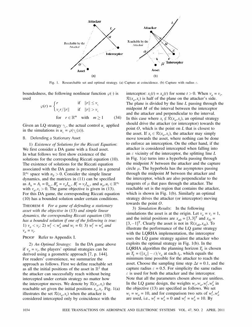
Fig. 1. Researchable set and optimal strategy. (a) Capture at coincidence. (b) Capture with radius ".

boundedness, the following nonlinear function '(¢) isused

'(r) =

½r if krk · v&v&r=krk if krk> v&for r 2Rm with m¸ 1 (34)

Given an LQ strategy °& , the actual control u& applied

in the simulations is u& = '(°&(x)).

B. Defending a Stationary Asset

1) Existence of Solutions for the Riccati Equation:

We first consider a DA game with a fixed asset.

In what follows we first show existence of the

solutions for the corresponding Riccati equation (10).

The existence of solutions for the Riccati equation

associated with the DA game is presented in a general

RnS space with nS > 0. Consider the simple lineardynamics, and the matrices in (11) can be specified

as Aa = Ai = 0nS , B0a = vaInS , B

0i = viInS , and ua,ui 2RnS

with va,vi > 0. The game objective is given in (13).

For this DA game, the corresponding Riccati equation

(10) has a bounded solution under certain conditions.

THEOREM 4 For a game of defending a stationary

asset with the objective in (13) and simple linear

dynamics, the corresponding Riccati equation (10)

has a bounded solution if one of the following is true:

1) va < vi; 2) wIi < w

Ia and wi = 0; 3) w

Ii = w

Ia and

va = vi.

PROOF Refer to Appendix I.

2) An Optimal Strategy: In the DA game above

if va = vi, the players’ optimal strategies can be

derived using a geometric approach [7, p. 144].

For readers’ convenience, we summarize the

approach as follows. First we define reachable set

as all the initial positions of the asset in R2 thatthe attacker can successfully reach without being

intercepted under certain strategy no matter how

the interceptor moves. We denote by R(xa,xi) thereachable set given the initial positions xa,xi. Fig. 1(a)

illustrates the set R(xa,xi) when the attacker isconsidered intercepted only by coincidence with the

interceptor: xi(t) = xa(t) for some t > 0. When va = vi,

R(xa,xi) is half of the plane on the attacker’s side.The plane is divided by the line L passing through the

midpoint M of the interval between the interceptor

and the attacker and perpendicular to the interval.

In this case where xt =2R(xa,xi), an optimal strategyshould drive the attacker (or interceptor) towards the

point O, which is the point on L that is closest to

the asset. If xt 2R(xa,xi), the attacker may simplymove towards the asset, where nothing can be done

to enforce an interception. On the other hand, if the

attacker is considered intercepted when falling into

an " vicinity of the interceptor, the splitting line L

in Fig. 1(a) turns into a hyperbola passing through

the midpoint N between the attacker and the capture

circle ¹. The hyperbola has the asymptotes passing

through the midpoint M between the attacker and

the interceptor, which are also perpendicular to the

tangents of ¹ that pass through the attacker. The

reachable set is the region that contains the attacker,

which is shown in Fig. 1(b). Similarly an optimal

strategy drives the attacker (or interceptor) moving

towards the point O.

3) Simulation Results: In the following

simulations the asset is at the origin. Let va = vi = 1,

and the initial positions are xa0 = [3,3]T and xi0 =

[3,¡1]T. Clearly the asset is not in R(xa0,xi0). Toillustrate the performance of the LQ game strategy

with the LQRHA implementation, the interceptor

uses the LQ game strategy against the attacker who

exploits the optimal strategy in Fig. 1(b). In the

LQRHA algorithm the planning horizon Tk is chosen

as Tk = (kxak¡ ")=va at each tk, which equals theminimum time possible for the attacker to reach the

asset. Choose the sampling time step ¢t= 0:1, and the

capture radius "= 0:5. For simplicity the same radius

" is used for both the attacker and the interceptor.

Note that all the parameters chosen above are unitless.

In the LQ game design, the weights wi,wa,wIi ,w

Ia in

the objective (13) are specified as follows. We set

wi = wa = 10, and for comparison two sets of wIi ,w

Ia

are used, i.e., wIi = wIa = 0 and w

Ii = w

Ia = 10. By


Fig. 2. Interception trajectories under LQ strategies with different wIi, wIa.

Fig. 3. Interception trajectories under interceptor's direct and optimal strategies.

Theorem 4, the corresponding Riccati equation (10)

has a bounded solution.

The simulated game trajectories with the strategies

specified above are shown in Fig. 2. With the LQRHA

implementation of the LQ strategies, the interceptor

can successfully intercept the attacker against its

optimal strategy. Regarding the difference induced

by the parameters wIi ,wIa, the strategy resulting from

larger wIi ,wIa performs better, and the attacker is

further away from the asset when intercepted. From

Table II, the interception also takes less time. With

positive wIi ,wIa, the interceptor appears to be more

aggressive and tracks the attacker more closely. This

is because of the effective penalty terms in the integral

in (7).

A suboptimal feedback strategy of the interceptor

udi =¡vi(xa¡ xi)=(kxa¡ xik) (xa 6= xi) is alsoconsidered. We call it “direct strategy.” This strategy

is referred to as a line-of-sight guidance law in missile

guidance, which drives the interceptor moving straight

towards the attacker. This is also an optimal pursuit

strategy in the PE game without the asset.

In the following simulations the interceptor uses

both the direct and the optimal strategy against the

attacker’s optimal strategy. The resulting players’

TABLE II

Inception/Attack Time Comparison

LQ LQ

Strategy Optimal (wIi,wIa = 10) (wI

i,wIa = 0) Direct

Interception/

Attack Time(s) 3.1 3.5 3.8 3.9

trajectories are illustrated in Fig. 3. The interceptor

fails to intercept the attacker under the direct strategy

because no prediction of the attacker’s movement

is available without taking into account the asset.

Since time is critical in a DA game, direct strategy is

disadvantageous. From the right plot of Fig. 3, when

both players use the optimal strategies, the players’

trajectories are straight lines. The interception time or

the time for the attacker to reach the asset is given in

Table II.

To better understand the impact from the design

parameters, we show by simulation how the design

parameters wa,wIa,wi,w

Ii can affect the performance

of the LQ strategies. To illustrate the influence

exclusively from the parameters wa,wi in (12), the

DA game with exactly the same initial conditions

and the simulation parameters is considered. The


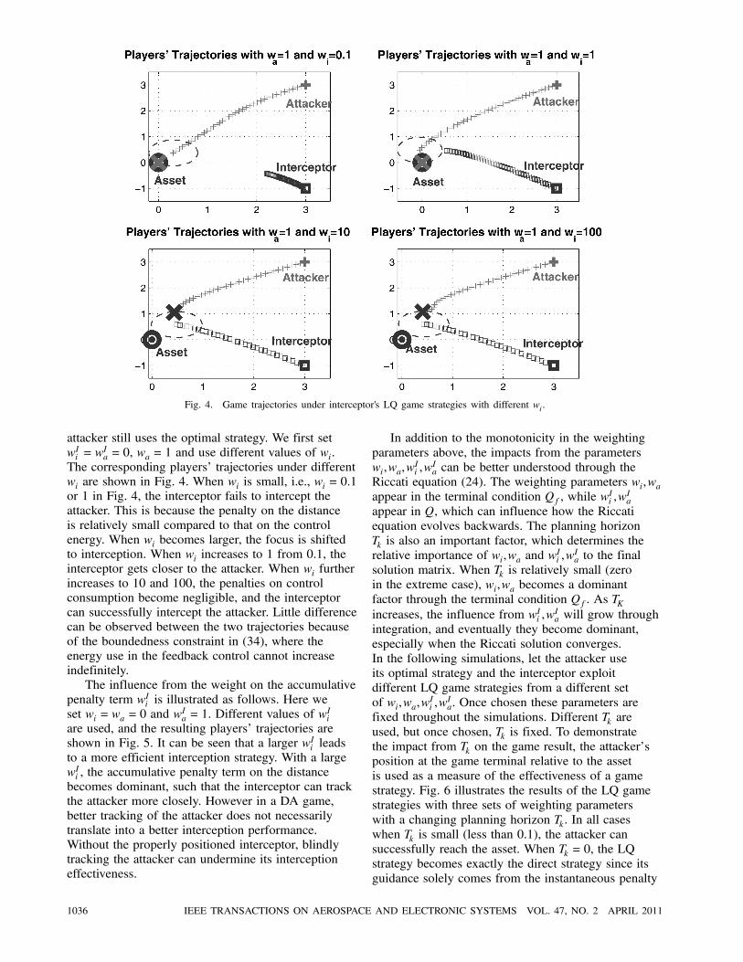
Fig. 4. Game trajectories under interceptor's LQ game strategies with different wi.

attacker still uses the optimal strategy. We first set

wIi = wIa = 0, wa = 1 and use different values of wi.

The corresponding players’ trajectories under different

wi are shown in Fig. 4. When wi is small, i.e., wi = 0:1

or 1 in Fig. 4, the interceptor fails to intercept the

attacker. This is because the penalty on the distance

is relatively small compared to that on the control

energy. When wi becomes larger, the focus is shifted

to interception. When wi increases to 1 from 0.1, the

interceptor gets closer to the attacker. When wi further

increases to 10 and 100, the penalties on control

consumption become negligible, and the interceptor

can successfully intercept the attacker. Little difference

can be observed between the two trajectories because

of the boundedness constraint in (34), where the

energy use in the feedback control cannot increase

indefinitely.

The influence from the weight on the accumulative

penalty term wIi is illustrated as follows. Here we

set wi = wa = 0 and wIa = 1. Different values of w

Ii

are used, and the resulting players’ trajectories are

shown in Fig. 5. It can be seen that a larger wIi leads

to a more efficient interception strategy. With a large

wIi , the accumulative penalty term on the distance

becomes dominant, such that the interceptor can track

the attacker more closely. However in a DA game,

better tracking of the attacker does not necessarily

translate into a better interception performance.

Without the properly positioned interceptor, blindly

tracking the attacker can undermine its interception

effectiveness.

In addition to the monotonicity in the weighting

parameters above, the impacts from the parameters

wi,wa,wIi ,w

Ia can be better understood through the

Riccati equation (24). The weighting parameters wi,waappear in the terminal condition Qf , while w

Ii ,w

Ia

appear in Q, which can influence how the Riccati

equation evolves backwards. The planning horizon

Tk is also an important factor, which determines the

relative importance of wi,wa and wIi ,w

Ia to the final

solution matrix. When Tk is relatively small (zero

in the extreme case), wi,wa becomes a dominant

factor through the terminal condition Qf . As TKincreases, the influence from wIi ,w

Ia will grow through

integration, and eventually they become dominant,

especially when the Riccati solution converges.

In the following simulations, let the attacker use

its optimal strategy and the interceptor exploit

different LQ game strategies from a different set

of wi,wa,wIi ,w

Ia. Once chosen these parameters are

fixed throughout the simulations. Different Tk are

used, but once chosen, Tk is fixed. To demonstrate

the impact from Tk on the game result, the attacker’s

position at the game terminal relative to the asset

is used as a measure of the effectiveness of a game

strategy. Fig. 6 illustrates the results of the LQ game

strategies with three sets of weighting parameters

with a changing planning horizon Tk. In all cases

when Tk is small (less than 0.1), the attacker can

successfully reach the asset. When Tk = 0, the LQ

strategy becomes exactly the direct strategy since its

guidance solely comes from the instantaneous penalty


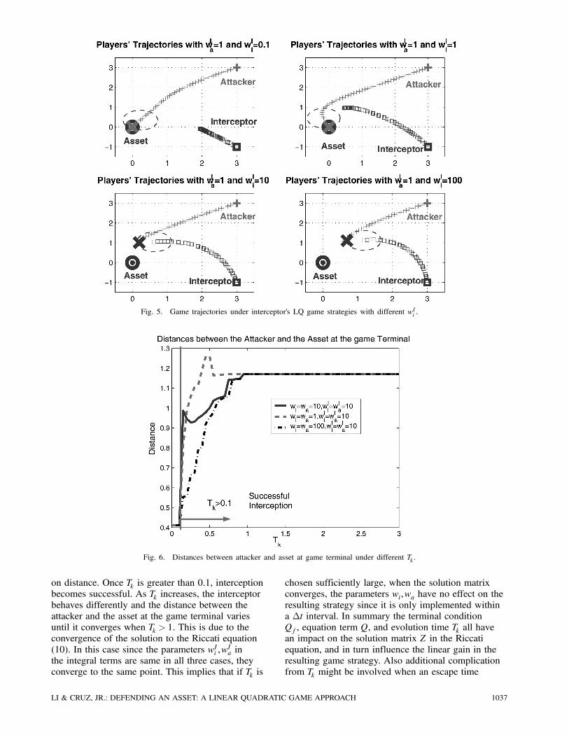
Fig. 5. Game trajectories under interceptor's LQ game strategies with different wIi.

Fig. 6. Distances between attacker and asset at game terminal under different Tk .

on distance. Once Tk is greater than 0.1, interception

becomes successful. As Tk increases, the interceptor

behaves differently and the distance between the

attacker and the asset at the game terminal varies

until it converges when Tk > 1. This is due to the

convergence of the solution to the Riccati equation

(10). In this case since the parameters wIi ,wIa in

the integral terms are same in all three cases, they

converge to the same point. This implies that if Tk is

chosen sufficiently large, when the solution matrix

converges, the parameters wi,wa have no effect on the

resulting strategy since it is only implemented within

a ¢t interval. In summary the terminal condition

Qf , equation term Q, and evolution time Tk all have

an impact on the solution matrix Z in the Riccati

equation, and in turn influence the linear gain in the

resulting game strategy. Also additional complication

from Tk might be involved when an escape time


Fig. 7. Interception region I under different intercepter's strategies.

exists, which imposes a practical constraint on Tk.

In practice wi,wa,wIi ,w

Ia, and Tk need to be carefully

chosen jointly to achieve a desired game

performance.

Next we show the interception capability of

the LQ game strategy. Let the initial position of

the attacker be (3,3). We focus on a set of the

interceptor’s initial positions, from which it can

successfully intercept the attacker under different

strategies. Let us call the set “interception region” and

denote it by I. The interception set depends on thestrategies of both the attacker and the interceptors.

Suppose that the attacker exploits the optimal

geometric strategy. Under the LQ game strategies

associated with wa = wi = 10 and two different

sets of wIa,wIi (w

Ia = w

Ii = 0 and w

Ia = w

Ii = 10), we

calculate the interception regions. For comparison

the interception regions associated with the optimal

and the direct strategy from the interceptor are also

calculated. In Fig. 7, the perimeters of I underdifferent interceptor’s strategies are depicted. By

definition each interception region I (inside theperimeter) contains all the points from which the

interceptor can successfully intercept the attacker.

Clearly I associated with the interceptor’s optimalstrategy is the largest set. The sets I associated withthe LQ game strategies are only slightly smaller.

Again the direct strategy has the worst interception

performance. The results suggest that the LQ game

design with LQRHA algorithm can determine a fairly

good practical interception guidance law.

TABLE III

Simulation Parameters

Attacker Interceptor Asset

Speed 1.5 2

Initial Position (¡4:5,6) (¡9,¡9) (2,2)

Finally the LQRHA algorithm has also been

applied to determine the attacker’s strategies against

the interceptor’s optimal strategy, and similar results

have been observed.

C. Defending a Mobile Asset with an ArbitraryTrajectory

In this section we consider a DA problem with a

mobile asset that moves following a known trajectory.

The dynamic equations in (33) are considered, and the

asset’s movement is described as follows:

_xt = 0:5t

_yt =¡0:5t¡ 2sin³¼5t´:

The speeds and the initial positions of the players are

specified in Table III.

The LQ game approach with the LQRHA

algorithm is used to determine both the attacker’s

and the interceptor’s strategies. Note that the Riccati

equation associated with this DA game has a bounded

solution. Let the sampling time interval ¢t= 0:1

and "= 0:5. At each sampling time tk = t0 + k¢t, the


Fig. 8. Interception trajectories under LQ game strategies with different wIi.

optimization horizon Tk is chosen as

Tk =minf(kxa¡ xtk¡ ")=va, (kxi¡ xak¡ ")=vig:The weighting parameters in the objective function

(15) are chosen as wa = wIa = wi = 10. We simulate the

game under different values of wIi such as wIi = 1 and

wIi = 10.

Fig. 8 depicts the interception trajectories under

the LQ game strategies associated with different

wIi s with the LQRHA algorithm. With a relatively

small wIi , wIi = 1, the attacker succeeds in reaching

the asset, while when wIi = 10, the interceptor

can closely track and successfully intercept the

attacker. Similar to the previous games, a bigger wIitranslates into better tracking. Based on a number

of simulations, the LQ strategy with the LQRHA

algorithm can provide fairly good guidance laws

for both the attacker and the interceptor in this DA

game with a mobile asset moving along an arbitrary

trajectory.

D. Defending an Escaping Asset

In the following DA game with an escaping

asset, the players are moving with the simple motion

dynamics given in (33). Consider the objective in

(22). We first present a theorem on the existence of

solutions for the associated Riccati equation, which is

a counterpart of Theorem 4.

THEOREM 5 In the game of defending an escaping

asset with the objective function (22) and simple linear

dynamics (33), if va < vi and vt < va, the corresponding

Riccati equation (10) has a bounded solution for any

T > 0.

PROOF Readers are referred to Appendix II for a

proof.

TABLE IV

Simulation Parameters

Attacker Interceptor Asset

Speed 1 1 0.5

Initial Position (0,4) (0,¡4) (4,2:5)

Fig. 9. Illustration of asset's escaping strategy.

Before simulation we first analyze the possible

strategies of the players. The game parameters are

in Table IV. Recall the players’ optimal strategies

derived in Section VIB2. With the given initial

conditions, the reachable set of the attacker R(xa,xi)is in the half plane above the x axis. Thus if the

asset tries to escape, its best chance is to move

south to cross the x axis as shown in Fig. 9. In

this example, it takes at least 5 s for the asset to

cross the x axis at the point C. Considering the

attacker’s speed and its distance to point C, we

can see that the asset can barely escape from the

attacker.


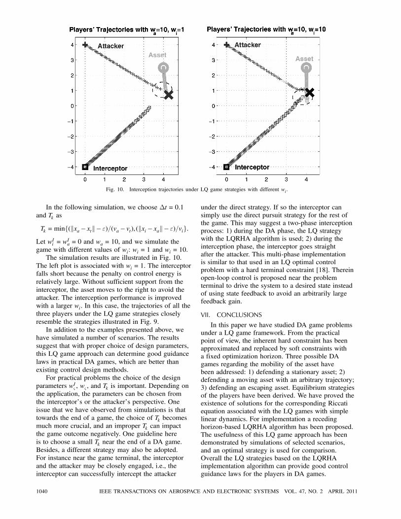
Fig. 10. Interception trajectories under LQ game strategies with different wi.

In the following simulation, we choose ¢t= 0:1

and Tk as

Tk =minf(kxa¡ xtk¡ ")=(va¡ vt), (kxi¡ xak¡ ")=vig:Let wIi = w

Ia = 0 and wa = 10, and we simulate the

game with different values of wi: wi = 1 and wi = 10.

The simulation results are illustrated in Fig. 10.

The left plot is associated with wi = 1. The interceptor

falls short because the penalty on control energy is

relatively large. Without sufficient support from the

interceptor, the asset moves to the right to avoid the

attacker. The interception performance is improved

with a larger wi. In this case, the trajectories of all the

three players under the LQ game strategies closely

resemble the strategies illustrated in Fig. 9.

In addition to the examples presented above, we

have simulated a number of scenarios. The results

suggest that with proper choice of design parameters,

this LQ game approach can determine good guidance

laws in practical DA games, which are better than

existing control design methods.

For practical problems the choice of the design

parameters wI& , w& , and Tk is important. Depending on

the application, the parameters can be chosen from

the interceptor’s or the attacker’s perspective. One

issue that we have observed from simulations is that

towards the end of a game, the choice of Tk becomes

much more crucial, and an improper Tk can impact

the game outcome negatively. One guideline here

is to choose a small Tk near the end of a DA game.

Besides, a different strategy may also be adopted.

For instance near the game terminal, the interceptor

and the attacker may be closely engaged, i.e., the

interceptor can successfully intercept the attacker

under the direct strategy. If so the interceptor can

simply use the direct pursuit strategy for the rest of

the game. This may suggest a two-phase interception

process: 1) during the DA phase, the LQ strategy

with the LQRHA algorithm is used; 2) during the

interception phase, the interceptor goes straight

after the attacker. This multi-phase implementation

is similar to that used in an LQ optimal control

problem with a hard terminal constraint [18]. Therein

open-loop control is proposed near the problem

terminal to drive the system to a desired state instead

of using state feedback to avoid an arbitrarily large

feedback gain.

VII. CONCLUSIONS

In this paper we have studied DA game problems

under a LQ game framework. From the practical

point of view, the inherent hard constraint has been

approximated and replaced by soft constraints with

a fixed optimization horizon. Three possible DA

games regarding the mobility of the asset have

been addressed: 1) defending a stationary asset; 2)

defending a moving asset with an arbitrary trajectory;

3) defending an escaping asset. Equilibrium strategies

of the players have been derived. We have proved the

existence of solutions for the corresponding Riccati

equation associated with the LQ games with simple

linear dynamics. For implementation a receding

horizon-based LQRHA algorithm has been proposed.

The usefulness of this LQ game approach has been

demonstrated by simulations of selected scenarios,

and an optimal strategy is used for comparison.

Overall the LQ strategies based on the LQRHA

implementation algorithm can provide good control

guidance laws for the players in DA games.


APPENDIX I. PROOF OF THEOREM 4

We first introduce some necessary notations.

Define H¢=fA,Q, Ba, Big, and denote by Ric[H](W)

the right-hand side of the Riccati equation in (10)

with matrix W of a proper dimension in place of

matrix Z. Define the set RH¢=fW 2Rn£n jW =WT

and Ric[H](W) 0g with 2 f¸,·,=g. We denote byW(¢,X0) the solution of (10) with W(t0,X0) = X0 forsome arbitrary and fixed t0. The following lemma is

needed to prove Theorem 4.

LEMMA 1 Suppose that there exist

W1 2 RH· and W2 2 RH¸ with W1 ·W2:Then W1 ·W0 ·W2 for some W0 2 Rn£n, and W0 =WT

0

yields that W(t,W0) exists for t 2 (¡1, t0] with W1 ·W1(t,W1)·W0(t,W0)·W2(t,W2)·W2 for t 2 (¡1, t0].PROOF Refer to Theorem 3.1 in [22] for a proof.

PROOF OF THEOREM 4 The proof of Theorem 4 is an

adaptation of Lemma 1. First of all the linear simple

dynamics in RnS can be rewritten in the form of (11)

with matrices A, Bi, Ba specified as

A= 02nS , Ba =

·vaInS

0

¸and Bi =

·0

viInS

¸:

Matrix Q1 in (14) is

Q1(wa,wi) =

·(wa¡wi)InS wiInS

wiInS ¡wiInS

¸such that Q,Qf in (13) can be determined accordingly.

Now we construct matrices W1 and W2 with the

properties specified in Lemma 1. Define

S¢= BaB

Ta ¡ BiBTi =

·v2aInS 0

0 ¡v2i InS

¸:

Let W1 be

W1¢=W11 +W12

¢=!11

·¡InS InS

InS ¡InS

¸+!12

·0 0

0 ¡InS

¸with parameters !11,!

12 ¸ 0 to be determined.

Substitute W1 into Ric[H] (with H¢=fA,Q, Bi, Bag), and

we obtain

Ric[H](W1) =¡Q+W1SW1 =¡Q+W11SW11 +W12SW12 +W11SW12 +W12SW11

=¡·(wIa¡wIi )InS wIi InS

wIi InS ¡wIi InS

¸+!112 (v

2a ¡ v2i )

·InS ¡InS¡InS InS

¸+!122

·0 0

0 ¡v2i InS

¸+!11!

12

·0 v2i InS

v2i InS ¡2v2i InS

¸: (35)

For any x= [xTa ,xTi ]T,

xTRic[H](W1)x= wIi kxi¡ xak2¡wIakxak2

+!121 (v2a ¡ v2i )kxi¡ xak2¡!122 v2i kxik2

¡ 2!11!12v2i kxik2 +2!11!12v2i xTi xa:(36)

Next we show that for each of the three cases in

Theorem 4, it is true that xTRic[H](W1)x· 0 forcertain !11,!

12. First if va < vi, we choose !

12 = 0, and

then (36) becomes

xTRic[H](W1)x

= wIi kxi¡ xak2¡wIakxak2 +!121 (v2a ¡ v2i )kxi¡ xak2:Note that va < vi, and clearly, we can choose !

11

sufficiently large such that xTRic[H](W1)x· 0 for anyx 2 R2nS . Secondly if wIi < wIa, we can choose !11 = 0,and similarly (36) becomes

xTRic[H](W1)x= wIi kxi¡ xak2¡wIakxak2¡!122 v2i kxik2:

Since wIi < wIa, we can choose !

12 sufficiently large

such that xTRic[H](W1)x· 0 for any x 2 R2nS . Thirdlyif wIi = w

Ia and va = vi, (36) becomes

xTRic[H](W1)x= wIi kxik2¡ 2wIi xTi xa¡!122 v2i kxik2

¡2!11!12v2i kxik2 +2!11!12v2i xTi xa:Now we choose !11,!

12 such that !

11!

12v2i = w

Ii , and

clearly xTRic[H](W1)x· 0. So far we have shown thatthere exists some W1 such that W1 2 RH· for each case.Now we check whether Qf ¸W1. Given any

x 2 R2nS ,xT(Qf ¡W1)x= (!11 ¡wi)kxi¡ xak2 +wakxak2 +!12kxak2:

(37)

It can be easily checked that for each of the cases

mentioned above, xT(Qf ¡W1)x¸ 0 with a proper !11.That is, Qf ¸W1.Next we construct matrix W2 as

W2 =

·!2InS 0nS

0nS 0nS

¸(38)

with parameter !2 > 0 to be determined. For the

matrix Ric[H](W2) =¡Q+W2SW2, given any


x= [xTa ,xTi ]T,

xTRic[H](W2)x

= (!22v2a ¡wIa+wIi )kxak2 +wIi kxik2¡ 2wIi xTa xi:

Clearly there exists some C1 > 0, such that when

!2 ¸ C1, xTRic[H](W2)x¸ 0 for any x 2R2nS , i.e.,W2 2 RH¸ . Furthermore for any x= [xTa ,xTi ]T,xT(W2¡Qf)x= (!2¡wa+wi)kxak2¡ 2wixTa xi+wikxik2:

There exists some C2 > 0 such that when !2 ¸ C2,xT(W2¡Qf)x¸ 0 for any x 2R2nS , i.e., W2 ¸Qf . Let!2 ¸maxfC1,C2g. Hence W1 ·Qf ·W2. By Lemma 1,a bounded solution exists for all t· T with T <1.

APPENDIX II. PROOF OF THEOREM 5

PROOF The proof is similar to that for Theorem 4 in

Appendix I. We can construct matrices

W1 = !1

264¡InS InS 0

InS ¡InS 0

0 0 0nS

375

W2 = !2

264 InS 0 ¡InS0 0nS 0

¡InS 0 InS

375with some !1,!2 ¸ 0 to be determined. It can be easilyshown, as in the proof for Theorem 4, Lemma 1

applies with proper !1 and !2. Thus a bounded

solution exists for all t · T with T <1.REFERENCES

[1] Hespanha, J., Prandini, M., and Sastry, S.

Probabilistic pursuit-evasion games: A one-step nash

approach.

In Proceedings of the 39th IEEE Conference on Decision

and Control, Sydney, Australia, 2000, 2272—2277.

[2] Schenato, L., Oh, S., and Sastry, S.

Swarm coordination for pursuit evasion games using

sensor networks.

In Proceedings of the International Conference on Robotics

and Automation, Barcelona, Spain, 2005, 2493—2498.

[3] Li, D. and Cruz, Jr., J. B.

Improvement with look-ahead on cooperative pursuit

games.

In Proceedings of the 44th IEEE Conference on Decision

and Control, San Diego, CA, Dec. 2006.

[4] Li, D., Cruz, Jr., J. B., and Schumacher, C.

Stochastic multi-player pursuit-evasion differential games.

International Journal of Robust and Nonlinear Control, 18

(2008), 218—247.

[5] Cruz, Jr., J. B., Simaan, M., Gacic, A., Jiang, H.,

Letellier, B., and Li, M.

Game-theoretic modeling and control of a military air

operation.

IEEE Transactions on Aerospace and Electronic Systems,

37, 4 (2001), 1393—1405.

[6] Cruz, Jr., J. B., Simaan, M., Gacic, A., and Liu, Y.

Moving horizon nash strategies for a military air

operation.


38, 3 (2002), 989—999.

[7] Isaacs, R.

Dfferential Games: A Mathematical Theory with

Applications to Warfare and Pursuit.

New York: Wiley, 1965.

[8] Basar, T. and Olsder, G.

Dynamic Noncooperative Game Theory (2nd ed.).

Philadelphia: SIAM, 1998.

[9] Ho, Y. C., Bryson, Jr., A. E., and Baron, S.

Differential games and optimal pursuit-evasion strategies.

IEEE Transactions on Automatic Control, AC-10, 4 (1965),

385—389.

[10] Willman, W.

Formal solutions for a class of stochastic pursuit-evasion

games.

IEEE Transactions on Automatic Control, 14, 5 (1969),

504—509.

[11] Turetsky, V. and Shinar, J.

Missile guidance laws based on pursuit-evasion game

formulations.

Automatica, 39, 4 (2003), 607—618.

[12] Liu, Y., Cruz, Jr., J. B., and Schumacher, C.

Pop-up threat models for persistent area denial.


43, 2 (2007), 509—521.

[13] Pachter, M.

Simple-motion pursuit-evasion in the half plane.

Computers & Mathematics with Applications, 13, 1—3

(1987), 69—82.

[14] Zarchan, P.

Tactical and Strategic Missile Guidance.

Reston, VA: American Institute of Aeronautics and

Astronautics, 2007.

[15] Evans, L. and Souganidis, P.

Differential games and representation formulas for

solutions of Hamilton-Jacobi-Isaacs equations.

Indiana University Mathematics Journal, 33, 5 (1984),

773—797.

[16] Fleming, W. and Souganidis, P.

On the existence of value functions of two-player,

zero-sum stochastic differential games.

Indiana University Mathematics Journal, 38, 2 (1989),

293—314.

[17] Mitchell, I., Bayen, A., and Tomlin, C.

A time-dependent Hamilton-Jacobi formulation of

reachable sets for continuous dynamic games.

IEEE Transactions on Automatic Control, 50, 7 (2005),

947—957.

[18] Bryson, Jr., A. E.

Dynamic Optimization.

Menlo Park, CA: Addison-Wesley Longman, 1999.

[19] Basar, T. and Bernhard, P.

H 1-optimal Control and Related Minimax DesignProblems (2nd ed.).

Boston: Birkhauser, 1995.

[20] Engwerda, J.

LQ Dynamic Optimization and Differential Games.

Hoboken, NJ: Wiley, 2005.

[21] Anderson, B. and Moore, J.

Optimal Control: Linear Quadratic Methods.

Upper Saddle River, NJ: Prentice-Hall, 1989.

[22] Freiling, G. and Jank, G.

Existence and comparison theorems for algebraic

Riccati equations and Riccati differential and difference

equations.

Journal of Dynamical and Control Systems, 2, 4 (1996),

529—547.


Dongxu Li received the B.S. degree in engineering physics from Tshinghua

University in 2000, P.R. China, the M.S. degree in mechanical engineering,

and the Ph.D. degree in electrical engineering from The Ohio State University,

Columbus, OH, in 2002 and 2006, respectively.

He is currently working as a researcher in R&D at General Motors Company.

Before joining GM, he was a postdoctoral researcher in the Department

of Electrical and Computer Engineering at The Ohio State University. His

research interests include control theory and applications in automotive systems,

cooperative control of networked systems, and dynamic game theory.


Jose B. Cruz, Jr. received the B.S. in electrical engineering from the University

of the Philippines (UP), April 1953, S.M. in electrical engineering from the

Massachusetts Institute of Technology (MIT), June 1956, and the Ph.D. in

electrical engineering from the University of Illinois, Urbana—Champaign,

October 1959.

He is a Distinguished Professor of Engineering and a Professor of Electrical

and Computer Engineering at The Ohio State University (OSU). Previously,

he served as Dean of the College of Engineering at OSU from 1992 to 1997,

and as a Professor of Electrical and Computer Engineering at the University of

California in Irvine (UCI) from 1986 to 1992 and at the University of Illinois

from 1965 to 1986. He was a visiting professor at MIT and Harvard University

in 1973 and visiting associate professor at the University of California, Berkeley

in 1964—1965. He served as instructor at UP 1953—1954 and research assistant at

MIT, 1954—1956.

Dr. Cruz, Jr., is the author or coauthor of six books, 23 chapters in

research books, and more than 250 articles in research journals and refereed

conference proceedings. He was elected a member of the National Academy

of Engineering (NAE) in 1980, Chair of the NAE Electronic Engineering Peer

Committee 2003, NAE Membership Committee 2003—2007, and he was elected

a corresponding member of the National Academy of Science and Technology

(NAST, Philippines) in 2003. He is a Fellow of the American Association for

the Advancement of Science (AAAS), elected 1989; a Fellow of the American

Society for Engineering Education (ASEE), elected in 2004; a Fellow of IFAC,

elected in 2007; recipient, Curtis W. McGraw Research Award of ASEE,

1972; recipient, Halliburton Engineering Education Leadership Award, 1981;

Distinguished Member, IEEE Control Systems Society, designated in 1983;

recipient, IEEE Centennial Medal, 1984; recipient, IEEE Richard M. Emberson

Award, 1989; recipient, ASEE Centennial Medal, 1993; and recipient, Richard E.

Bellman Control Heritage Award, American Automatic Control Council (AACC),

1994.

In addition to membership in ASEE, AAAS, NAE, NAST, he is a member

of the Institute for Operations Research and Management Science (INFORMS),

the Philippine American Association for Science and Engineering (PAASE,

Founding member 1980, Founding President-Elect 1981, Chairman of the Board

1998—2000), Philippine Engineers and Scientists Organization (PESO), National

Society of Professional Engineers (NSPE), Sigma Xi, Phi Kappa Phi, and Eta

Kappa Nu.

He has served on various professional society boards and editorial boards,

and he served as an officer of professional societies, including IEEE wherein he

was President of the IEEE Control Systems Society in 1979, Editor of the IEEE

Transactions on Automatic Control, a member of the IEEE Board of Directors

from 1980 to 1985, IEEE Vice President for Technical Activities in 1982 and

1983, and IEEE Vice President for Publication Activities in 1984 and 1985. He

served as Chair of the Engineering Section of AAAS in 2004—2005. He served as

a member of the Board of Examiners for Professional Engineers for the State of

Illinois, 1984—1986.


defending an asset: a linear quadratic game approach

Documents