deepdive: a data management system for automatic knowledge ... · deepdive: a data management...
TRANSCRIPT
DeepDive: A Data Management System for
Automatic Knowledge Base Construction
by
Ce Zhang
A dissertation submitted in partial fulfillment of
the requirements for the degree of
Doctor of Philosophy
(Computer Sciences)
at the
UNIVERSITY OF WISCONSIN–MADISON
2015
Date of final oral examination: 08/13/2015
The dissertation is approved by the following members of the Final Oral Committee:
Jude Shavlik, Professor, Computer Sciences (UW-Madison)
Christopher Re, Assistant Professor, Computer Science (Stanford University)
Jeffrey Naughton, Professor, Computer Sciences (UW-Madison)
David Page, Professor, Biostatistics and Medical Informatics (UW-Madison)
Shanan Peters, Associate Professor, Geosciences (UW-Madison)

c© Copyright by Ce Zhang 2015
All Rights Reserved

i
ACKNOWLEDGMENTS
I owe Christopher Re my career as a researcher, the greatest dream of my life. Since the day I first met
Chris and told him about my dream, he has done everything he could, as a scientist, an educator, and
a friend, to help me. I am forever indebted to him for his completely honest criticisms and feedback,
the most valuable gifts an advisor can give. His training equipped me with confidence and pride that
I will carry for the rest of my career. He is the role model that I will follow. If my whole future career
achieves an approximation of what he has done so far in his, I will be proud and happy.
I am also indebted to Jude Shavlik and Miron Livny, who, after Chris left for Stanford, kindly
helped me through all the paperwork and payments at Wisconsin. If it were not for their help, I
would not have been able to continue my PhD studies. I am also profoundly grateful to Jude for
being the chair of my committee. I am also likewise grateful to Jeffrey Naughton, David Page, and
Shanan Peters for serving on my committee; and Thomas Reps for his feedback during defense.
DeepDive would have not been possible without all its users. Shanan Peters was the first user,
working with it before it even got its name. He spent three years going through a painful process with
us before we understood the current abstraction of DeepDive. I am grateful to him for sticking with
us for this long process. I would also like to thank all the scientists and students who have interacted
with me, without whose generous sharing of knowledge we could not have refined DeepDive to its
current state. A very incomplete list includes Gabor Angeli, Gill Bejerano, Noel Heim, Arun Kumar,
Pradap Konda, Emily Mallory, Christopher Manning, Jonathan Payne, Eldon Ulrich, Robin Valenza,
and Yuke Zhu. DeepDive is now a team effort, and I am grateful to the whole DeepDive team,
especially Jaeho Shin and Michael Cafarella, who help in managing the DeepDive team.
I am also extremely lucky to be surrounded by my friends. Heng Guo, Yinan Li, Linhai Song, Jia
Xu, Junming Xu, Wentao Wu, and I have lunch frequently whenever we are in town, and this often
amounts to the happiest hour in the entire day. Heng, a theoretician, has also borne the burden of
listening to me pitch my system ideas for years, simply because he is, unfortunately for him, my
roommate. Feng Niu mentored me through my early years at Wisconsin; even today, whenever I
struggle to decide what the right thing to do is, I still imagine what he would have done in a similar
situation. Victor Bittorf sparked my interest in modern hardware through his beautiful code and lucid
tutorial. Over the years, I learned a lot from Yinan and Wentao about modern database systems, from
Linhai about program analysis, and from Heng about counting.
Finally, I would also like to thank my parents for all their love over the last twenty-seven years
and, I hope, in the future. Anything that I could write about them in any languages, even in my
native Chinese, would pale beside everything they have done to support me in my life.
My graduate study has been supported by the Defense Advanced Research Projects Agency
(DARPA) Machine Reading Program under Air Force Research Laboratory prime contract No. FA8750-
09-C-0181, the DARPA DEFT Program under No. FA8750-13-2-0039, the National Science Foundation
(NSF) EAGER Award under No. EAR-1242902, and the NSF EarthCube Award under No. ACI-
1343760. Any opinions, findings, and conclusions or recommendations expressed in this material are
those of the authors and do not necessarily reflect the views of DARPA, NSF, or the U.S. government.

ii
The results mentioned in this dissertation come from previously published work [16,84,90,148,157,171,204–207]. Some descriptions are directly from these papers. These papers are joint efforts with differentauthors, including: F. Abuzaid, G. Angeli, V. Bittorf, V. Govindaraju, S. Gupta, S. Hadjis, M. Premkumar,A. Kumar, M. Livny, C. Manning, F. Niu, C. Re, S. Peters, C. Sa, A. Sadeghian, Z. Shan, J. Shavlik, J. Shin,J. Tibshirani, F. Wang, J. Wu, and S. Wu. Although this dissertation bears my name, this collection ofresearch would not have been possible without the contributions of all these collaborators.

iii
ABSTRACT
Many pressing questions in science are macroscopic: they require scientists to consult information
expressed in a wide range of resources, many of which are not organized in a structured relational
form. Knowledge base construction (KBC) is the process of populating a knowledge base, i.e., a
relational database storing factual information, from unstructured inputs. KBC holds the promise of
facilitating a range of macroscopic sciences by making information accessible to scientists.
One key challenge in building a high-quality KBC system is that developers must often deal with
data that are both diverse in type and large in size. Further complicating the scenario is that these
data need to be manipulated by both relational operations and state-of-the-art machine-learning
techniques. This dissertation focuses on supporting this complex process of building KBC systems.
DeepDive is a data management system that we built to study this problem; its ultimate goal is
to allow scientists to build a KBC system by declaratively specifying domain knowledge without
worrying about any algorithmic, performance, or scalability issues.
DeepDive was built by generalizing from our experience in building more than ten high-quality
KBC systems, many of which exceed human quality or are top-performing systems in KBC competi-
tions, and many of which were built completely by scientists or industry users using DeepDive. From
these examples, we designed a declarative language to specify a KBC system and a concrete protocol
that iteratively improves the quality of KBC systems. This flexible framework introduces challenges
of scalability and performance–Many KBC systems built with DeepDive contain statistical inference
and learning tasks over terabytes of data, and the iterative protocol also requires executing similar
inference problems multiple times. Motivated by these challenges, we designed techniques that make
both the batch execution and incremental execution of a KBC program up to two orders of magnitude
more efficient and/or scalable. This dissertation describes the DeepDive framework, its applications,
and these techniques, to demonstrate the thesis that it is feasible to build an efficient and scalable
data management system for the end-to-end workflow of building KBC systems.

iv
SOFTWARE, DATA, AND VIDEOS
• DeepDive is available at http://deepdive.stanford.edu. It is a team effort to further develop
and maintain this system.
• The DeepDive program of PaleoDeepDive (Chapter 4) is available at http://deepdive.stanford.
edu/doc/paleo.html and can be executed with DeepDive v0.6.0α.
• The code for the prototype systems we developed to study the tradeoff of performance and
scalability is also available separately.
1. Elementary (Chapter 5.1): http://i.stanford.edu/hazy/hazy/elementary
2. DimmWitted (Chapter 5.2): http://github.com/HazyResearch/dimmwitted. This was
developed together with Victor Bittorf.
3. Columbus (Chapter 6.1): http://github.com/HazyResearch/dimmwitted/tree/master/
columbus. This was developed together with Arun Kumar.
4. Incremental Feature Engineering (Chapter 6.2): DeepDive v0.6.0α. This was developed
together with the DeepDive team, especially Jaeho Shin, Feiran Wang, and Sen Wu.
• Most data that we can legally release are available as DeepDive Open Datasets at deepdive.
stanford.edu/doc/opendata. The computational resources to produce these data are made
possible by millions of machine hours provided by the Center of High Throughput Computing
(CHTC), led by Miron Livny at UW-Madison.
• These introductory videos in our YouTube channel are related to this dissertation:
1. PaleoDeepDive: http://www.youtube.com/watch?v=Cj2-dQ2nwoY
2. GeoDeepDive: http://www.youtube.com/watch?v=X8uhs28O3eA
3. Wisci: http://www.youtube.com/watch?v=Q1IpE9_pBu4
4. Columbus: http://www.youtube.com/watch?v=wdTds3yg_G4
5. Elementary: http://www.youtube.com/watch?v=Zf7sgMnR89c and http://www.youtube.
com/watch?v=B5LxXGIkYe4

v
DEPENDENCIES OF READING
1
2.1 3 4
7 8
2.2 5 6
• If you are only interested in how DeepDive can be used to construct knowledge bases to help
your applications and example systems built with DeepDive, you can read following the red
solid line.
• If you are only interested in our work on efficient and scalable statistical analytics, you can read
following the blue dotted line.
• Otherwise, you can read in linear order.

vi
CONTENTS
Acknowledgments i
Abstract iii
Software, Data, and Videos iv
Dependencies of Reading v
Contents vi
List of Figures viii
List of Tables x
1 Introduction 1
1.1 Sample Target Workload . . . . . . . . . . . . . . . . . . . . . . . . . . . . . . . 2
1.2 The Goal of DeepDive . . . . . . . . . . . . . . . . . . . . . . . . . . . . . . . . 2
1.3 Technical Contributions . . . . . . . . . . . . . . . . . . . . . . . . . . . . . . . 4
2 Preliminaries 6
2.1 Knowledge Base Construction (KBC) . . . . . . . . . . . . . . . . . . . . . . . . 6
2.2 Factor Graphs . . . . . . . . . . . . . . . . . . . . . . . . . . . . . . . . . . . . . 12
3 The DeepDive Framework 17
3.1 A DeepDive Program . . . . . . . . . . . . . . . . . . . . . . . . . . . . . . . . . 18
3.2 Semantics of a DeepDive Program . . . . . . . . . . . . . . . . . . . . . . . . . . 21
3.3 Debugging and Improving a KBC System . . . . . . . . . . . . . . . . . . . . . . 27
3.4 Conclusion . . . . . . . . . . . . . . . . . . . . . . . . . . . . . . . . . . . . . . 31
4 Applications using DeepDive 32
4.1 PaleoDeepdive . . . . . . . . . . . . . . . . . . . . . . . . . . . . . . . . . . . . 33
4.2 TAC-KBP . . . . . . . . . . . . . . . . . . . . . . . . . . . . . . . . . . . . . . . . 54
5 Batch Execution 58
5.1 Scalable Gibbs Sampling . . . . . . . . . . . . . . . . . . . . . . . . . . . . . . . 59
5.2 Efficient In-memory Statistical Analytics . . . . . . . . . . . . . . . . . . . . . . 77
5.3 Conclusion . . . . . . . . . . . . . . . . . . . . . . . . . . . . . . . . . . . . . . 104
6 Incremental Execution 105
6.1 Incremental Feature Selection . . . . . . . . . . . . . . . . . . . . . . . . . . . . 106
6.2 Incremental Feature Engineering . . . . . . . . . . . . . . . . . . . . . . . . . . 131
6.3 Conclusion . . . . . . . . . . . . . . . . . . . . . . . . . . . . . . . . . . . . . . 147
vii
7 Related Work 148
7.1 Knowledge Base Construction . . . . . . . . . . . . . . . . . . . . . . . . . . . . 148
7.2 Performant and Scalable Statistical Analytics . . . . . . . . . . . . . . . . . . . . 151
8 Conclusion and Future Work 157
8.1 Deeper Fusion of Images and Text . . . . . . . . . . . . . . . . . . . . . . . . . . 157
8.2 Effective Solvers for Hard Constraints . . . . . . . . . . . . . . . . . . . . . . . . 159
8.3 Performant and Scalable Image Processing . . . . . . . . . . . . . . . . . . . . . 159
8.4 Conclusion . . . . . . . . . . . . . . . . . . . . . . . . . . . . . . . . . . . . . . 160
Bibliography 161
A Appendix 176
A.1 Scalable Gibbs Sampling . . . . . . . . . . . . . . . . . . . . . . . . . . . . . . . 176
A.2 Implementation Details of DimmWitted . . . . . . . . . . . . . . . . . . . . . . 178
A.3 Additional Details of Incremental Feature Engineering . . . . . . . . . . . . . . 180

viii
LIST OF FIGURES
1.1 An illustration of the input and output of a KBC system built for paleontology. . . . . . . 3
2.1 An illustration of the KBC model. . . . . . . . . . . . . . . . . . . . . . . . . . . . . . . . 7
2.2 An illustration of features extracted for a KBC system. . . . . . . . . . . . . . . . . . . . 9
2.3 A example of factor graphs. . . . . . . . . . . . . . . . . . . . . . . . . . . . . . . . . . . 12
2.4 An illustration of Gibbs sampling over factor graphs. . . . . . . . . . . . . . . . . . . . . 15
3.1 An example DeepDive program for a KBC system. . . . . . . . . . . . . . . . . . . . . . . 18
3.2 An illustration of the development loop of KBC systems. . . . . . . . . . . . . . . . . . . 19
3.3 Schematic illustration of grounding factor graphs in DeepDive. . . . . . . . . . . . . . . 22
3.4 Illustration of calibration plots automatically generated by DeepDive. . . . . . . . . . . 26
3.5 Error analysis workflow of DeepDive. . . . . . . . . . . . . . . . . . . . . . . . . . . . . . 29
4.1 Illustration of the PaleoDeepDive workflow (overall). . . . . . . . . . . . . . . . . . . . . 34
4.2 Illustration of the PaleoDeepDive workflow (statistical inference and learning). . . . . . 35
4.3 Image processing component for body size extraction in PaleoDeepDive. . . . . . . . . . 41
4.4 Relation extraction component for body size extraction in PaleoDeepDive. . . . . . . . . 41
4.5 Spatial distribution of PaleoDeepDive’s extraction (Overlapping Corpus). . . . . . . . . . 44
4.6 Spatial distribution of PaleoDeepDive’s extraction (Whole Corpus). . . . . . . . . . . . . 45
4.7 Machine- and human-generated macroevolutionary results. . . . . . . . . . . . . . . . . 47
4.8 Genus range end points genera common to the PaleoDB and PaleoDeepDive. . . . . . . . 49
4.9 Effect of changing PaleoDB training database size on PaleoDeepDive quality. . . . . . . . 50
4.10 Genus-level diversity generated by PaleoDeepDive for the whole document set. . . . . . 51
4.11 Lesion study of the size of knowledge base (random sample) in PaleoDeepDive. . . . . . 52
4.12 Lesion study of the size of knowledge base (chronological) in PaleoDeepDive. . . . . . . 53
4.13 The set of entities and relations in TAC-KBP competition. . . . . . . . . . . . . . . . . . . 55
5.1 Different materialization strategies for Gibbs sampling. . . . . . . . . . . . . . . . . . . . 63
5.2 Scalability of different systems for Gibbs sampling. . . . . . . . . . . . . . . . . . . . . . 72
5.3 Accuracy of cost model of different materialization strategies for Gibbs sampling. . . . . 73
5.4 I/O tradeoffs for Gibbs sampling. . . . . . . . . . . . . . . . . . . . . . . . . . . . . . . . 74
5.5 Illustration of DimmWitted for in-memory statistical analytics. . . . . . . . . . . . . . . . 81
5.6 Illustration of DimmWitted’s engine. . . . . . . . . . . . . . . . . . . . . . . . . . . . . . 84
5.7 Illustration of the method selection tradeoff in DimmWitted. . . . . . . . . . . . . . . . . 87
5.8 Illustration of model replication tradeoff in DimmWitted. . . . . . . . . . . . . . . . . . . 90
5.9 Illustration of data replication tradeoff in DimmWitted. . . . . . . . . . . . . . . . . . . . 91
5.10 Expeirments on tradeoffs in DimmWitted. . . . . . . . . . . . . . . . . . . . . . . . . . . 96
5.11 Lesion study of data access tradeoff in DimmWitted. . . . . . . . . . . . . . . . . . . . . 100
5.12 The impact of architectures and sparsity on model replication in DimmWitted. . . . . . . 102

ix
5.13 Lesion study of data replication tradeoff in DimmWitted. . . . . . . . . . . . . . . . . . . 103
6.1 Example snippet of a Columbus program. . . . . . . . . . . . . . . . . . . . . . . . . . . 110
6.2 Architecture of Columbus. . . . . . . . . . . . . . . . . . . . . . . . . . . . . . . . . . . . 111
6.3 The cost model of Columbus. . . . . . . . . . . . . . . . . . . . . . . . . . . . . . . . . . 115
6.4 An illustration of the tradeoff space of Columbus. . . . . . . . . . . . . . . . . . . . . . . 116
6.5 End-to-end performance of Columbus. . . . . . . . . . . . . . . . . . . . . . . . . . . . . 125
6.6 Robustness of materialization tradeoff in Columbus. . . . . . . . . . . . . . . . . . . . . 128
6.7 The impact of model caching in Columbus. . . . . . . . . . . . . . . . . . . . . . . . . . . 129
6.8 The performance of optimizer in Columbus. . . . . . . . . . . . . . . . . . . . . . . . . . 130
6.9 A summary of tradeoffs for incremental maintaince of factor graphs. . . . . . . . . . . . 137
6.10 Corpus statistics for incremental feature engineering. . . . . . . . . . . . . . . . . . . . . 140
6.11 Quality of incremental inference and learning . . . . . . . . . . . . . . . . . . . . . . . . 144
6.12 The tradeoff space of incremental feature engineering. . . . . . . . . . . . . . . . . . . . 146
8.1 A sample pathway in a diagram. . . . . . . . . . . . . . . . . . . . . . . . . . . . . . . . 158

x
LIST OF TABLES
3.1 Semantic of factor functions in factor graph. . . . . . . . . . . . . . . . . . . . . . . . . . 23
4.1 List of features and rules used in PaleoDeepDive. . . . . . . . . . . . . . . . . . . . . . . 36
4.2 List of sistant supervisionr rules used in PaleoDeepDive. . . . . . . . . . . . . . . . . . . 37
4.3 Statistics of the factor graphs on different corpora. . . . . . . . . . . . . . . . . . . . . . 45
4.4 Extraction statistics. . . . . . . . . . . . . . . . . . . . . . . . . . . . . . . . . . . . . . . 46
4.5 Statistics of lesion study on the size of knowledge base. . . . . . . . . . . . . . . . . . . . 52
5.1 I/O cost of Gibbs sampling with different materialization strategies. . . . . . . . . . . . . 63
5.2 Comparison of features of different systems for Gibbs sampling. . . . . . . . . . . . . . . 67
5.3 Data sets sizes for experiments of scalable Gibbs sampling. . . . . . . . . . . . . . . . . . 68
5.4 Different configurations of experiments for scalable Gibbs sampling. . . . . . . . . . . . 69
5.5 Performance of scalable Gibbs sampling. . . . . . . . . . . . . . . . . . . . . . . . . . . . 70
5.6 Size of materialized state for scalable Gibbs sampling. . . . . . . . . . . . . . . . . . . . 73
5.7 A summary of access methods in DimmWitted. . . . . . . . . . . . . . . . . . . . . . . . 83
5.8 Summary of machine and bandwidths used to test DimmWitted. . . . . . . . . . . . . . . 84
5.9 A summary of DimmWitted’s tradeoffs and existing systems. . . . . . . . . . . . . . . . . 85
5.10 Comparison of different access methods in DimmWitted. . . . . . . . . . . . . . . . . . . 86
5.11 Dataset statistics for experiments of DimmWitted . . . . . . . . . . . . . . . . . . . . . . 93
5.12 Performance of DimmWitted and other systems. . . . . . . . . . . . . . . . . . . . . . . . 94
5.13 Comparison of throughput of DimmWitted and other systems. . . . . . . . . . . . . . . . 99
5.14 Plan that DimmWitted chooses in the tradeoff space. . . . . . . . . . . . . . . . . . . . . 99
6.1 A summary of tradeoffs in Columbus. . . . . . . . . . . . . . . . . . . . . . . . . . . . . . 108
6.2 A summary of operators in Columbus. . . . . . . . . . . . . . . . . . . . . . . . . . . . . 111
6.3 Dataset and program statistics of experiments for Columbus. . . . . . . . . . . . . . . . 124
6.4 Statistics of KBC systems for experiments of incremental feature engineering. . . . . . . 141
6.5 The set of rules used in experiments of incremental feature engineering . . . . . . . . . 141
6.6 End-to-end efficiency of incremental inference and learning. . . . . . . . . . . . . . . . . 143

1
1. Introduction
Science is built up of facts, as a house is with stones.
— Jules Henri Poincare, La Science et l’Hypothese, 1901
Knowledge Base Construction (KBC) is the process of populating a knowledge base (KB), i.e., a
relational database storing factual information, from unstructured and/or structured input, e.g., text,
tables, or even maps and figures. Because of its potential to answer key scientific questions, for
decades, KBC has been conducted by scientists in various domains, such as the global compendia
of marine animals compiled by Sepkoski in 1981 [167], the PaleoBioDB1 project for biodiversity,
and the PharmGKB [94] project for pharmacogenomics. The knowledge bases constructed by these
projects contain up to one million facts and have contributed to hundreds of scientific discoveries.2
Despite their usefulness, it is typical for these knowledge bases to require a large amount of human
resources to construct. For example, the PaleoBioDB project was constructed by an international
group of more than 380 scientists with approximately nine continuous person years [148]. Partially
motivated by the cost of building KBs manually, Automatic Knowledge Base Construction3 has recently
received tremendous interest from both academia [23,32,48,71,105,134,149,170,179,200] and
industry [73,112,133,192,209]. It is becoming clear that one key requirement for building a high-
quality KBC system is to support processing data that are both diverse in type (e.g., text and tables)
and large in size (e.g., larger than terabytes) with both relational operations and state-of-the-art
machine learning techniques. One challenge introduced by this requirement is how to help domain
scientists manage the complexity caused by these sophisticated operations and diverse data sources.
This dissertation demonstrates the thesis that it is feasible to build a data management system to
support the end-to-end workflow of building KBC systems; moreover, by providing such an integrated
framework, we gain benefits that are otherwise harder to achieve. We build DeepDive to demonstrate
this thesis. In this chapter, we first present examples of the KBC workload; then, we present the goal
of our study, and the technical contributions.
1paleobiodb.org/#/2paleobiodb.org/#/publications; www.pharmgkb.org/view/publications-pgkb.do3In the remaining part of this document, we use the term KBC to refer to an automatic KBC system.

2
1.1 Sample Target Workload
We present examples of KBC systems to illustrate the target workload that we focus on in this
dissertation. The goal for this section is not to provide a complete description of the workload but
instead to provide enough information to guide the reader through the rest of the chapter. A detailed
description and examples of KBC workload are the topics of Chapter 2 and Chapter 4.
As illustrated in Figure 1.1, the input to a KBC system are resources such as journal articles, and
the output is a relational database filled in with facts that can be supported by the input resources.
For example, if a KBC system is given as an input a text snippet from a journal article that stating,
“The Namurian Tsingyuan Formation from Ningxia, China is divided into three members,” it could
produce the following extractions. First, it could extract the phrase “Tsingyuan Formation” refers to a
rock formation, “Ningxia, China” refers to a location, and “Namurian” refers to a temporal interval of
age 326 to 313 million years. It will also extract relations between rock formation and their location
and age as illustrated in Figure 1.1(a). Similar extractions can be extracted from other sources of
input, such as tables, images, or even document layouts, as illustrated in Figure 1.1(b-d).
DeepDive has been used to build more than ten KBC systems similar to the one illustrated above,
and these systems form the basis on which we justify our design decisions in DeepDive. In this
dissertation, we focus on five KBC systems that the author of this dissertation involved in building for
paleontology [148], geology [206], Freebase-like relations [16], genomics, and pharmacogenomics.
These KBC systems have achieved high quality in these domains: the paleontology system has
been featured in Nature [46] and achieves quality equal to (and sometimes better than) human
experts [148], and the Freebase-like KBC system was the top-performing system for TAC-KBP 2014
slot-filling task. As DeepDive has become more mature recently, the development of KBC systems has
been done more and more by domain scientists instead of the builder of DeepDive in its early stage.
1.2 The Goal of DeepDive
To achieve high quality in the process as illustrated above, an automatic KBC system is often designed
to take advantage of multiple (noisy) input data sources, existing knowledge bases and taxonomies,
domain knowledge from scientists, state-of-the-art natural language processing tools, and, as a
growing trend, machine learning and statistical inference and learning. As a result, these KBC
systems often need to deal with diverse types of data, and a diverse set of operations to manipulate

3
… The Namurian Tsingyuan Formation
from Ningxia, China, is divided into
three members …
(a) Natural Language Text
Formation Time
Tsingyuan Fm. Namurian
Formation-Time (Location)
Taxon Formation
Retispira Tsingyuan Fm.
Taxon-Formation
Taxon Taxon
StrobeusRectilinea
BuccinumRectineum
Taxon-Taxon
Taxon Real Size
Shansiellatongxinensis
5cm x 5cm
Taxon-Real Size
(b) Table
Formation Location
Tsingyuan Fm. Ningxia
(c) Document Layout (d) Image
Figure 1.1: An illustration of the input and output of a KBC system built for paleontology.
the data. Apart from the diversity of data sources and operations, it is also typical for KBC systems to
deal with Web-scale data sets and statistical operations that are not relational.
The goal of this thesis is to help domain experts, who want to build a KBC system, to deal with
the sheer volume and diversity of data and operations required in KBC. Therefore, DeepDive is
designed to be a data management system, which, if successful, will allow domain experts to build a
KBC system by declaratively specifying domain knowledge without worrying about any algorithmic,
performance, or scalability issues.

4
1.3 Technical Contributions
We divide the techniques of this dissertation into three categories.
(1) An Abstraction of General Workflow of KBC Systems. As the first step in building DeepDive, we
focus on providing an abstraction to model the KBC workload. Ideally, this abstraction should support
most common operations that users use while building KBC systems. To come up with this abstraction,
we conducted case studies to build KBC systems in a diverse set of domains [16,84,148,206]. Based
on our observations from these case studies, we designed the execution model of DeepDive to consist
of three phases: (1) feature extraction, (2) probabilistic knowledge engineering, and (3) statistical
inference and learning. Given this execution model, to build a KBC system with DeepDive, domain
experts first specify each of these phases with a declarative language, and iteratively improve each
phase to achieve high quality. The first contribution is a Datalog-like language that allows domain
experts to specify these three phases, and an iterative protocol to guide domain experts on debugging
and improving each phase [157,171]. This language and protocol has been applied to more than ten
KBC systems, and the simplicity and flexibility of this language allows it to be used by users who are
not computer scientists. This is the topic of Chapter 3 and Chapter 4.
(2) Performant and Scalable Statistical Inference and Learning. Given the three-phase frame-
work of DeepDive, the next focus is to make each phase performant and scalable. One design decision
we made is to rely on relational databases whenever possible, which allows us to take advantage
of decades of study by the database community to speed up and scale up the feature extraction
and probabilistic engineering phase. Therefore, this dissertation mainly focuses on speeding up and
scaling up the statistical inference and learning phase that contains non-relational operations seen in
statistical analytics, e.g., generalized linear models and Gibbs sampling. The second contribution is
the study of (1) speeding up a subset of statistical analytics models on modern multi-socket, multi-
core, non-uniform memory access (NUMA) machines with SIMD instructions when these models
fit in the main memory [207]; and (2) scaling up a subset of statistical analytics models when the
model does not fit in the main memory [206]. These techniques enable improvement of up to two
orders of magnitude on the performance and scalability of these operations, which, together with
classic relational techniques, helps to free the domain experts from worrying about the performance
and scalability issues in building KBC systems with DeepDive. This is the topic of Chapter 5.
5
(3) Performant Iterative Debugging and Development. A common development pattern in KBC,
as we observed in case studies, is that building a KBC system is an iterative exploratory process. That
is, a domain expert often executes a set of different, but similar, KBC systems to find suitable features,
input sources, and domain knowledge to use. Therefore, the last focus of this dissertation is to further
optimize this iterative development pattern by supporting incremental execution of a KBC system.
The technical challenge is that some operations in KBC are not relational, and, therefore, classic
techniques developed for incrementally maintaining relational database systems cannot be used
directly. The third contribution is to develop techniques to speed up exploratory feature selection and
engineering with generalized linear models [204] and statistical inference and learning [171]. These
techniques provide a speedup of another two orders of magnitude on the real workload we observed
in KBC systems built by DeepDive users. This is the topic of Chapter 6.
Summary The central goal of this dissertation is to introduce a system, DeepDive, that can support
the end-to-end workflow of building KBC systems to deal with inputs that are both diverse and large
in size. DeepDive aims at supporting the thesis of this work, that is it is feasible to build a data
management system to support the end-to-end workflow of building KBC systems; moreover, by providing
such an integrated framework, we gain benefits that are otherwise harder to achieve. The main technical
challenges are (1) what abstraction this system should provide to non-CS domain scientists, and (2)
the performance in executing a KBC system built with this abstraction. For the first challenge, we
design the framework by generalizing from more than ten KBC systems that we built in the past; and
for the second challenge, we study techniques of both batch execution and incremental execution.

6
2. Preliminaries
In this chapter, we describe two pieces of critical background material for this thesis:
1. A walkthough on what a KBC system is, specifically, (1) concrete examples of KBC systems;
(2) a KBC model that is an abstraction of objects used in KBC systems; and (3) a list of common
operations that the user conducts while building KBC systems. The goal of this part is not to
describe the technique or abstraction of DeepDive but, rather to get to the same page regarding
the type of systems and workload we want to support with DeepDive.
2. A description of the factor graph, a type of probabilistic graphical model that is the abstraction
we used for statistical inference and learning. The goal is to set up the notation and definition
that the rest of this document will consistently exploit.
2.1 Knowledge Base Construction (KBC)
The input to a KBC system is a heterogeneous collection of unstructured, semi-structured, and
structured data, ranging from text documents to existing but incomplete KBs. The output of the
system is a relational database containing facts extracted from the input and put into the appropriate
schema. Creating the knowledge base may involve extraction, cleaning, and integration.
Example 2.1. Figure 1.1(a) shows a knowledge base with pairs of rock formations and locations that
the rock formation is found. The input to the system is a collection of journal articles published in
paleontology journals; the output is a KB containing pairs of rock formations and their location. In
this example, a KBC system populates the KB with linguistic patterns, e.g., ‘... from ...’ between a pairs
of mentions (e.g., “Tsingyuan Fm” and “Ningxia”). As we will see later, these linguistic patterns are
called features in DeepDive, and roughly, these features are then put in a classifier deciding whether
this pair of mentions indicates that a formation appears in a location (in the Formation-Location)
relation. KBC systems can also populate knowledge bases from resources other than natural language text.
Figure 1.1(b-d) illustrate examples of KBC systems built to extract information from tables, document

7
Entities Corpus
Relationships
Mr. Gates was the CEO of Microsoft.
Google acquired YouTube in 2006.
Company Founder
Microsoft Corp. Bill Gates
… …
FoundedBy
Acquirer Acquiree
Google Inc. YouTube
… …
Acquired
Person
Bill Clinton
Bill Gates
Steve Jobs
Barack Obama
Organization
Google Inc.
Microsoft Corp.
United States
YouTube
Relation Mentions
EntityMentions
Figure 2.1: An illustration of the KBC model.
layout, and image. In practice, it is not uncommon for scientists to require a KBC system to deal with all
these resources to answer their scientific questions [148].
Example 2.1 shows a KBC system for paleontology. Similar examples can also be found in other
domains. For example, considering a knowledge base with pairs of individuals that are married to
each other. In this case, The input to the system is a collection of news articles and an incomplete set
of married persons; the output is a KB containing pairs of person that are married. A KBC system
extracts linguistic patterns, e.g., “... and his wife ...” between a pair of mentions of individuals
(e.g.,“Barack Obama” and “M. Obama”) to decide whether this pair of mentions indicates that they
are married (in the HasSpouse) relation. As another example, in pharmacogenomics, scientists might
want to populate a knowledge base with pairs of gene and drug that interacts with each other by
extracting features from journal articles. These similar examples of KBC systems in different domains
can be characterized by (1) a KBC model, and (2) a list of common operations executed over the
KBC model. We now describe these two parts in details.
2.1.1 The KBC Model
As we can see from Example 2.1, a KBC system needs to interact with different data sources. A
KBC model is the abstraction of these data sources. We adopt standard KBC model that has been

8
developed by the KBC community for decades and used in standard KBC competitions, e.g., ACE.1
There are four types of objects that a KBC system seeks to extract from input documents, namely
entities, relations, mentions, and relation mentions.
1. Entity: An entity is a real-world person, place, or thing. For example, the entity “Michelle Obama 1”
represents the actual entity for a person whose name is “Michelle Obama”.
2. Relation: A relation associates two (or more) entities, and represents the fact that there
exists a relationship between these entities. For example, the entity “Barack Obama 1” and
“Michelle Obama 1” participate in the HasSpouse relation, which indicates that they are married.
3. Mention: a mention is a span of text in an input document that refers to an entity or rela-
tionship: “Michelle” may be a mention of the entity “Michelle Obama 1.” An entity might
have mentions of different from; for example, apart from “Michelle”, mentions of the form
“M. Obama” or “Michelle Obama” can also refer to the same entity “Michelle Obama 1.” The
process of mapping mentions to entities is called entity linking.
4. Relation Mention: A relation mention is a phrase that connects two mentions that participate
in a relation, e.g., the phrase “and his wife” that connects the mentions “Barack Obama” and
“M. Obama”.
Figure 2.1 illustrates the examples and the relationship between these four types of objects. As
we will see later in Chapter 3, DeepDive provides an abstraction to represent each type of objects as
database relations and random variables, and provides a language for the user to specify indicators
and the correlations between these objects.
2.1.2 Common Operations of KBC
Section 2.1.1 shows a data model of different types of objects inside a KBC system, and we now
describe a set of operations a KBC system needs to support over this data model. This list of operations
come from our our observations from the users of DeepDive while building different KBC systems.
1http://www.itl.nist.gov/iad/mig/tests/ace/2000/

9
Journal Articles
… The Namurian Tsingyuan Formation from
Ningxia, China, is divided into three members …
Text
OCR
NLP
The Namurian Tsingyuan Formation from Ningxiann
detnn
prep pobj
Entity1 Entity2 Feature
Namurian Tsingyuan Fm. nn
Silesian Tsingyuan Fm. SameRow
Relational Features SQL+Python
Existing ToolsTableAge Formation
Silesian Tsingyuan
Figure 2.2: An illustration of features extracted for a KBC system.
Feature Extraction. The concept of a feature is one of the most important concepts for building
KBC systems. We already see some example of features in Example 2.1; we now describe feature
extraction in more details.
To extract features, the user specifies a mapping that takes as input both structured and un-
structured information, and output features associated with entities, mentions, relations, or relation
mentions. Intuitively, each feature will then be used as “evidience” to make prediction about the asso-
ciated object. For example, Figure 2.2 illustrates features extracted for predicting relation mentions
between temporal intervals and rock formations.
Given the diversity of input sources and target domains, the features extracted by the user is also
higely diverse. For example:
• The user might need to run existing tools, such as Optical Character Recognition (OCR) and
Natural Language Processing (NLP) tools to acquire information from text, HTML, or images.
The output might contain JSON objects to represent parse trees or DOM structures.
• The user might also write user defined functions (UDF) in their favorite languages, e.g., Python,
Perl, or SQL, to further process the information produced by existing tools. Examples include
the word sequence features between two mentions as we see in Example 2.1, or the features
derived from parse trees or table structures as illustrated in Figure 2.2.

10
One should notice that different features might be different regarding how “strong” they are as
indicators of the target task. For example, the feature “... wife of ...” between two mentions could be
a strong indicator of the HasSpouse relation, while the feature “... met ...” is much weaker. As we will
see later in Chapter 3, DeepDive provides a way for the user to write these feature extractors, and
automatically learn the weight, i.e., strengths, of features from training example provided by the user.
Domain Knowledge Integration. Another way to improve the quality of KBC systems is to integrate
knowledge specific to the application domain. Such knowledge are assertions that are (statistically)
true in the domain. Examples include
• To help extract the HasSpouse relation between persons, one can integrate the knowledge that
“One person is likely to be the spouse of only one person.”
• To help extract the HasAge relation between rock formations and temporal intervals, one can
integrate the knowledge that “The same rock formation is not likely to have ages spanning 100
million years long.”
• To help extract the BodySize relation between species and size measurements, one can integrate
the knowledge that “Adult T. Rex are larger than humans.”
• To help extract the HasFormula relation between chemical names and chemical formulae, one
can integrate the knowledge that “C as in benzene can only make four chemical bonds.”
To see how domain knowledge helps KBC systems, consider the effect of integrating the rule
“one person is likely to be the spouse of only one person.” With this rule, given a single entity
“Barack Obama,” this rule gives positive preference to the case where only one of (Barack Obama,
Michelle Obama) and (Barack Obama, Michelle Williams) is true. Therefore, even if the KBC system
makes a wrong prediction about (Barack Obama, Michelle Williams) according to a wrong feature or
a misleading document, integrating domain knowledge provides the opportunities to correct this.
One should also notice from this example that domain knowledge does not need to be always
correct to be useful. As we will see later in Chapter 3, DeepDive provides a way for the user to
specify her “confidence” of domain knowledge by either manually specifying or letting DeepDive
automatically learn a real-valued weight.

11
Supervision. As we have described in previous paragraphs, both the features extracted and domain
knowledge integrated need a weight to indicate how strong an indicator they are to the target task.
One way to do that is for the user to manually specify the weight, which we support in DeepDive;
however, another more easy, consistent, and effective way is for DeepDive to automatically learn the
weight with machine learning techniques.
One challenge with building a machine learning system for KBC is collecting on training examples.
As the number of predicates in the system grows, specifying training examples for each relation
is tedious and expensive. Although DeepDive supports the standard supervised machine learning
paradigm in which the user provides manually labelled training example, another common technique
to cope with this is distant supervision. Distant supervision starts with an (incomplete) entity-level
knowledge base and a corpus of text. The user then defines a (heuristic) mapping between entities
in the database and text. This map is used to generate (noisy) training data for mention-level
relations [61,96,131]. We illustrate this procedure by an example.
Example 2.2 (Distant Supervision). Consider the mention-level relation HasSpouse. To find training
data, we find sentences that contain mentions of pairs of entities that are married, and we consider the
resulting sentences positive examples. Negative examples could be generated from pairs of persons who
are, say, parent-child pairs. Ideally, the patterns that occur between pairs of mentions corresponding to
mentions will contain indicators of marriage more often than those that are parent-child pairs (or other
pairs). Selecting those indicative phrases or features allows us to find features for these relations and
generate training data. Of course, engineering this mapping is a difficult task in practice and requires
many iterations.
One should notice that the training examples generated by distant supervision are not necessarily
always real training examples of the relation. For example, the fact that we see “Barack Obama”
and “Michelle Obama” in the same sentence does not necesarily mean that this sentence contains
linguistic indicator of the HasSpouse relation. The hope of distant supervision is that, statistically
speaking, most distantly generated training examples are correct. As we will see later in Chapter 3,
DeepDive provides a way for the user to write distant supervision rules as relational mappings.
Iterative Refinement As the reader might already notice, all of the above three operations do not
necessarily produce completely correct data. In the meantime, we observe that KBC systems built

12
Raw Data
He said that he will submit a paper.
v1 v2 v3 v4
Factor Graph
v1
v2
v3
v4
He
said
that
he
c1
c2
c3
c4
Adjacent-tokenfactors
Same-wordfactors
In-database Representation
User Relations Correlation Relationsvid wordv1 Hev2 saidv3 thatv4 he
fid varsc1 (v1,v2)c2 (v2,v3)c3 (v3,v4)
fid varsc4 (v1,v4)
F1
F2
An Example Assignment σ
Assignmentvid assignmentv1 1v2 0v3 0v4 1
Partition Function𝑍 𝐼𝜎 = 𝑓' 1,0 × 𝑓' 0,0 × 𝑓' 0,1 × 𝑓, (1,1)
Factors in F1
Factors in F2
Figure 2.3: An example factor graph that represents a simplified skip-chain CRF; more sophisticatedversions of this model are used in named-entity recognition and parsing. There is one user relationcontaining all tokens, and there are two correlation relations for adjacent-token correlation (F1) andsame-word correlation (F2) respectively. The factor function associated to F1 (resp. F2), called f1
(resp. f2), is stored in a manner similar to a user-defined function.
with DeepDive achieves higher than 95% accuracy, sometimes even higher than human experts on
the same task, with these imperfect data. These two facts together might look counter-intuitive –
How can a system make accurate predictions with less accurate data?
Part of this is achieved by iteratively improving the above three phases by the user of DeepDive to
eliminate noise that matters. For example, the user might look at the errors made by a KBC system,
and refine her feature extractors, domain knowledge, or ways of generating distantly supervised
training examples. As we will see later in Chapter 3, DeepDive provides a concrete protocol for the
user to follow in this iterative refinement process. It also provides different ways for the user to
diagnose different reasons of errors made in a KBC system.
2.2 Factor Graphs
As we will see later in Chapter 3, DeepDive heavily relies on factor graphs, one type of probabilistic
graphical models, for its statistical inference and learning phase. We present preliminaries on factor
graphs, and the inference and learning operations over factor graphs.

13
Factor graphs have been used to model complex correlations among random variables for
decades [188], and have recently been adopted as one underlying representation for probabilistic
databases [165,189,194]. In this work, we describe factor graph following the line of work of proba-
bilistic databases; and the reader can find other types of formalization in classic textbooks [111,188].
We first describe the definition of a factor graph, and then how to do inference and learning over
factor graphs with Gibbs sampling.
2.2.1 Factor Graphs
A key principle of factor graphs is that random variables should be separated from the correlation
structure. Following this principle, we define a probabilistic database to be D = (R,F), where R
is called the user schema and F is called the correlation schema. Relations in the user schema (resp.
correlation schema) are called user relations (resp. correlation relations). A user’s application interacts
with the user schema, while the correlation schema captures correlations among tuples in the user
schema. Figure 2.3 gives a schematic view of the concepts in this section.
User Schema Each tuple in a user relation Ri ∈ R has a unique tuple ID, which takes values from
a variable ID domain D, and is associated with a random variable2 taking values from a variable value
domain V. We assume that V is Boolean. For some random variables, their value may be fixed as
input, and we call these variables evidence variables. We denote the set of positive evidence variables
as P ⊆ D, and the set of negative evidence variables as N ⊆ D. Each distinct variable assignment
σ : D 7→ V defines a possible world Iσ that is equivalent to a standard database instantiation of the
user schema. We say a variable assignment is consistent with P and N if it assigns True for all variables
in P and False for all variables in N. Let I be the set of all possible worlds, and Ie be the set of all
possible worlds that are consistent with evidence P and N.
Correlation Schema The correlation schema defines a probability distribution over the possible
worlds as follows. Intuitively, each correlation relation Fj ∈ F represents one type of correlation over
the random variables in D by specifying which variables are correlated and how they are correlated.
To specify which, the schema of Fj has the form Fj(fid, v) where fid is a unique factor ID taking
values from a factor ID domain F, and v ∈ Daj where aj is the number of random variables that
2Either modeling the existence of a tuple (for Boolean variables) or in the form of a special attribute of Ri.

14
are correlated by each factor.3 In Figure 2.3, variables v1 and v4 are correlated. To specify how,
Fj is associated with a function fj : Vaj 7→ R and a real-number weight wj . Given a possible
world Iσ, for any t = (fid, v1, . . . , vaj ) ∈ Fj , define gj(t, Iσ) = wjfj(σ(v1), . . . , σ(vaj )). Define
vars(fid) = v1, . . . , vaj. To explain independence in the graph, we need the notion of the Markov
blanket [146,188] of a variable v, denoted mb(v), and defined to be
mb(vi) = v | v 6= vi, ∃fid ∈ F s.t. v, vi ⊆ vars(fid).
In Figure 2.3, mb(v1) = v2, v4. In general, a variable v is conditionally independent of a variable
v′ 6∈mb(v) given mb(v). Here, v1 is independent of v3 given v2, v4.
Probability Distribution Given I, the set of all possible worlds, we define the partition function
Z : I 7→ R+ over any possible world I ∈ I as
Z(I) = exp
∑Fj∈F
∑t∈Fj
gj(t, I)
(2.1)
The probability of a possible world I ∈ I is
Pr[I] = Z(I)
(∑J∈I
Z(J)
)−1
. (2.2)
It is well known that this representation can encode all discrete distributions over possible worlds [24].
2.2.2 Inference and Query Answering
In a factor graph, which defines a probability distribution, (marginal) inference refers to the process of
computing the probability that a random variable will take a particular value. Marginal inference on
factor graphs is a powerful framework. For each variable vi, let I+e be all possible worlds consistent
with evidences in which vi is assigned to True and I−e be all possible worlds consistent with evidences
in which vi is assigned to False, the marginal probability of vi is defined as
Pr[vi] =
∑I∈I+e Z(I)∑
I∈I+e Z(I) +∑I∈I−e Z(I)
3Our representation supports factors with varying arity as well, but we focus on fixed-arity factors for simplicity.

15
Previous State Next StateSample
c1
c2
c3
c4
Variable Factor
0
1
0
1
v1
v2
v3
v4
c1
c2
c3
c4
Variable Factor
0
1
1
1
v1
v2
v3
v4
𝑝 = Pr 𝑣& = 1 𝑣( = 1,𝑣* = 1
= 𝑓, 1,1 ×𝑓, 1,1 ×
𝑓, 1,0 ×𝑓, 0,1 + 𝑓, 1,1 ×𝑓, 1,1
1,
With probability 𝑝 set 𝑣& = 1
Current variable
0 Assignment
Figure 2.4: A step of Gibbs sampling. To sample a variable v3, we read the current values of variablesin mb(v3) = v2, v4 and calculate the conditional probability Pr[v3|v2, v4]. Here, the sample resultis v3 = 1. We update the value of v3 and then proceed to sample v4.
Gibbs Sampling As exact inference for factor graphs is well-known to be intractable [146,188], a
commonly used inference approach is to sample, and then use the samples to compute the marginal
probabilities of random variables (e.g., by averaging the outcomes). The main idea of Gibbs sampling
is as follows. We start with a random possible world I0. For each variable v ∈ D, we sample a new
value of v according to the conditional probability Pr[v|mb(v)]. A routine calculation shows that
computing this probability requires that we retrieve the assignment to the variables in mb(v) and the
factor functions associated with the factor nodes that neighbor v. Then we update v in I0 to the new
value. After scanning all variables, we obtain a first sample I1. We repeat this to get Ik+1 from Ik.
Example 2.3. We continue our example (see Figure 2.3) of skip-chain conditional random field [182],
a type of factor graphs used in named-entity recognition [74]. Figure 2.4 illustrates one step in Gibbs
sampling to update a single variable, v3: we compute the probability distribution over v3 by retrieving
factors c2 and c3, which determines mb(v3). Then, we find the values of v2 and v4. Using Equation 2.2,
one can check that the probability that v3 = 1 is given by the equation in Figure 2.4 (conditioned on
mb(v3), the remaining factors cancel out).
There are several popular optimization techniques for Gibbs sampling. One class of techniques
improves the sample quality, e.g., burn-in, in which we discard the first few samples, and thinning, in
which we retain every kth sample for some integer k [15]. A second class of techniques improves
throughput using parallelism. The key observation is that variables that do not share factors may be

16
sampled independently and so in parallel [197]. These techniques are essentially orthogonal to our
contributions, and we do not discuss them further in this dissertation.
2.2.3 Weight Learning
Another operation over factor graph is to learn the weight associated with each factor. Given the set
of possible worlds that are consistent with evidences Ie, weight learning tries to find the weight that
maximizes the probability of these possible worlds
arg maxwj
∑I∈Ie Z(I)∑I∈I Z(I)
There are different ways of solving this optimization problem, and they are out of the scope of this
dissertation. In DeepDive, we follow the standard procedure of stochastic gradient descent and
estimate the gradient with samples draw with Gibbs sampling [111,188].
2.2.4 Discussion
In DeepDive, the default algorithm implemented for inference and learning is Gibbs sampling and
stochastic gradient descent. However, there are many other well-studied approaches that can be
used to solve the problem of inference and learning over factor graphs, e.g., junction trees [111],
log-determinant relaxation [187], or belief propagation [188], etc. In principle, these approaches
could be implemented and plug in directly into DeepDive just as different solvers. We do not discuss
them in this dissertation because they are orthogonal to the contributions of DeepDive.

17
3. The DeepDive Framework
The world that I was programming in back then has passed, and the goal now is for things to be
easy, self-managing, self-organizing, self-healing, and mindless. Performance is not an issue.
Simplicity is a big issue.
— Jim Gray, An Interview by Marianne Winslett, 2002
In this chapter, we present DeepDive, a data management system built to support the KBC workload
as described in Chapter 2.1. The goal of DeepDive is to provide a simple, but flexible, framework for
domain experts to deal with diverse types of data and integrate domain knowledge. This chapter is
organized as follows:
1. DeepDive Program. We describe DeepDive program, the program that the user writes to build
a KBC system. A DeepDive program allows the user to specify features, domain knowledge,
and distant supervision, all in an unified framework.
2. Semantic and Execution of DeepDive Programs. Given a DeepDive program, we define its
semantics and how it is executed in DeepDive.
3. Debugging a DeepDive Program. Building a KBC system is an iterative process, and we
describe a concrete protocol that the user can follow to improve a KBC system via repeated
error analysis.
In this chapter, our focus is to define at a high level how DeepDive supports the KBC workload,
and how a real KBC system is built with DeepDive. We do not discuss the specific techniques that
make the execution and debugging of DeepDive programs performant and scalable, which will be the
topics of Chapter 5 and Chapter 6.

18
B. Obama and Michelle were married in 1992.
(1a) Unstructured Information
Malia and Sasha Obama attended the state dinner.
(1b) Structured Information
Tunicia and Raleigh Hall were married in June.
Person1 Person2
Barack Obama
Michelle Obama
… …
HasSpouse
(2) User Schema
SID Content
S1 B. Obama and Michelle were married in 1992.
Sentence (documents)
EID1 EID2
BarackObama
Michelle Obama
Married
MID1 MID2 VALUE
M1 M2 true
MarriedMentions_Ev
SID MID
S1 M2
PersonCandidate
SID MID WORD
S1 M2 Michelle
Mentions
MID EID
S2 Michelle Obama
EL
MID1 MID2
M1 M2
MarriedCandidate
(3a) Candidate Generation and Feature Extraction
(R1) MarriedCandidate(m1,m2) :- PersonCandidate(s,m1), PersonCandidate(s,m2)
(FE1) MarriedMentions(m1,m2) :- MarriedCandidate(m1,m2), Sentence(sid,sent), Mentions(s,m1,w1), Mentions(s,m2,w2), weight=phrase(m1,m2,sent)
(3b) Supervision Rule
(S1) MarriedMentions_Ev(m1,m2,true) :- MarriedCandidate(m1,m2), Married(e1,e2),EL(m1,e1), EL(m2,e2),
Figure 3.1: An example DeepDive program for a KBC system.
3.1 A DeepDive Program
DeepDive is an end-to-end framework for building KBC systems, as shown in Figure 3.2.1 We walk
through each phase. DeepDive supports both SQL and Datalog, but we use Datalog syntax for
exposition. The rules we describe in this section are manually created by the user of DeepDive and
the process of creating these rules is application-specific.
Candidate Generation and Feature Extraction All data in DeepDive is stored in a relational
database. The first phase populates the database using a set of SQL queries and user-defined functions
(UDFs) that we call feature extractors. By default, DeepDive stores all documents in the database in
one sentence per row with markup produced by standard NLP pre-processing tools, including HTML
1For more information, including examples, please see http://deepdive.stanford.edu. Note that our engine is builton Postgres and Greenplum for all SQL processing and UDFs. There is also a port to MySQL.

19
... Barack Obama and his wife M. Obama ...
1.8M Docs
Engineering-in-the-loop Development
Feat
ure
Ext.
rule
s
New
doc
umen
ts
Infe
renc
e ru
les
Supe
rvis
ion
rule
s
Upd
ated
KB
Erro
r an
alys
is
add…
Input
Candidate Generation & Feature Extraction
Supervision Learning & Inference
3 Hours 1 Hours 3 Hours
KBC System Built with DeepDive
2.4M Facts
Output
HasSpouse
Figure 3.2: A KBC system takes as input unstructured documents and outputs a structured knowledgebase. The runtimes are for the TAC-KBP competition system (News). To improve quality, the developeradds new rules and new data.
stripping, part-of-speech tagging, and linguistic parsing. After this loading step, DeepDive executes
two types of queries: (1) candidate mappings, which are SQL queries that produce possible mentions,
entities, and relations, and (2) feature extractors that associate features to candidates, e.g., “... and
his wife ...” in Example 2.1.
Example 3.1. Candidate mappings are usually simple. Here, we create a relation mention for every pair
of candidate persons in the same sentence (s):
(R1) MarriedCandidate(m1,m2) : -
PersonCandidate(s,m1), PersonCandidate(s,m2).
Candidate mappings are simply SQL queries with UDFs.2 Such rules must be high recall: if the
union of candidate mappings misses a fact, DeepDive has no chance to extract it.
We also need to extract features, and we extend classical Markov Logic in two ways: (1) user-
defined functions and (2) weight tying, which we illustrate by example.
Example 3.2. Suppose that phrase(m1,m2, sent) returns the phrase between two mentions in the
2These SQL queries are similar to low-precision but high-recall ETL scripts.

20
sentence, e.g., “and his wife” in the above example. The phrase between two mentions may indicate
whether two people are married. We would write this as:
(FE1) MarriedMentions(m1,m2) : -
MarriedCandidate(m1,m2), Mention(sid,m1),
Mention(sid,m2), Sentence(sid, sent)
weight = phrase(m1,m2, sent).
One can think about this like a classifier: This rule says that whether the text indicates that the mentions
m1 and m2 are married is influenced by the phrase between those mention pairs. The system will infer
based on training data its confidence (by estimating the weight) that two mentions are indeed indicated
to be married.
Technically, phrase returns an identifier that determines which weights should be used for a
given relation mention in a sentence. If phrase returns the same result for two relation mentions,
they receive the same weight. We explain weight tying in more detail later. In general, phrase
could be an arbitrary UDF that operates in a per-tuple fashion. This allows DeepDive to support
common examples of features such as “bag-of-words” to context-aware NLP features to highly domain-
specific dictionaries and ontologies. In addition to specifying sets of classifiers, DeepDive inherits
Markov Logic’s ability to specify rich correlations between entities via weighted rules. Such rules are
particularly helpful for data cleaning and data integration.
Supervision DeepDive can use training data or evidence about any relation; in particular, each
user relation is associated with an evidence relation with the same schema and an additional field
that indicates whether the entry is true or false. Continuing our example, the evidence relation
MarriedMentions Ev could contain mention pairs with positive and negative labels. Operationally,
two standard techniques generate training data: (1) hand-labeling, and (2) distant supervision, which
we illustrate below.
Example 3.3. Distant supervision [61,96,131] is a popular technique to create evidence in KBC systems.
The idea is to use an incomplete KB of married entity pairs to heuristically label (as True evidence) all
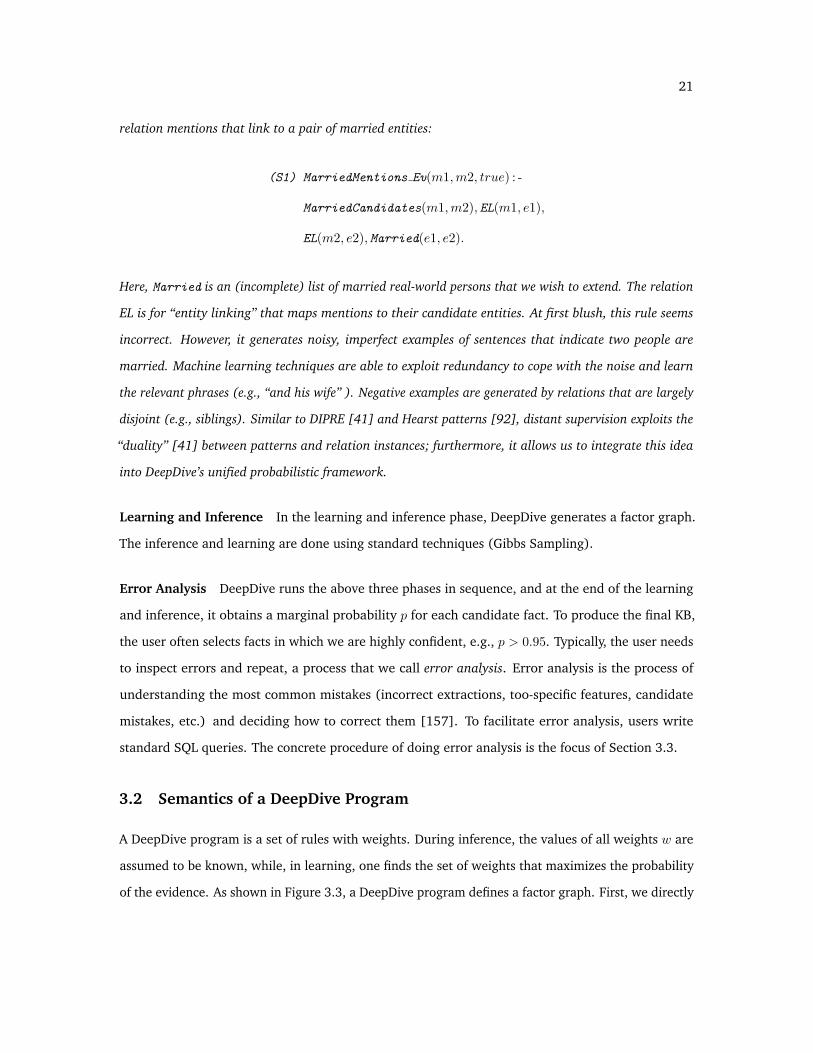
21
relation mentions that link to a pair of married entities:
(S1) MarriedMentions Ev(m1,m2, true) : -
MarriedCandidates(m1,m2), EL(m1, e1),
EL(m2, e2), Married(e1, e2).
Here, Married is an (incomplete) list of married real-world persons that we wish to extend. The relation
EL is for “entity linking” that maps mentions to their candidate entities. At first blush, this rule seems
incorrect. However, it generates noisy, imperfect examples of sentences that indicate two people are
married. Machine learning techniques are able to exploit redundancy to cope with the noise and learn
the relevant phrases (e.g., “and his wife” ). Negative examples are generated by relations that are largely
disjoint (e.g., siblings). Similar to DIPRE [41] and Hearst patterns [92], distant supervision exploits the
“duality” [41] between patterns and relation instances; furthermore, it allows us to integrate this idea
into DeepDive’s unified probabilistic framework.
Learning and Inference In the learning and inference phase, DeepDive generates a factor graph.
The inference and learning are done using standard techniques (Gibbs Sampling).
Error Analysis DeepDive runs the above three phases in sequence, and at the end of the learning
and inference, it obtains a marginal probability p for each candidate fact. To produce the final KB,
the user often selects facts in which we are highly confident, e.g., p > 0.95. Typically, the user needs
to inspect errors and repeat, a process that we call error analysis. Error analysis is the process of
understanding the most common mistakes (incorrect extractions, too-specific features, candidate
mistakes, etc.) and deciding how to correct them [157]. To facilitate error analysis, users write
standard SQL queries. The concrete procedure of doing error analysis is the focus of Section 3.3.
3.2 Semantics of a DeepDive Program
A DeepDive program is a set of rules with weights. During inference, the values of all weights w are
assumed to be known, while, in learning, one finds the set of weights that maximizes the probability
of the evidence. As shown in Figure 3.3, a DeepDive program defines a factor graph. First, we directly

22
User Relations
Inference Rules
Factor Graph
Variables VR S Q
Q(x) :- R(x,y)
Q(x) :- R(x,y), S(y)
F1 F2Factors F
Factor function corresponds toEquation 3.1 in Section 3.2.
Grounding
x ya 0a 1a 2
r1
r2
r3
s1
s2
y0
10
q1
xa r1 r2 r3 s1 s2 q1
F1
F2
Figure 3.3: Schematic illustration of grounding. Each tuple corresponds to a Boolean random variableand node in the factor graph. We create one factor for every set of groundings.
define the probability distribution for rules that involve weights, as it may help clarify our motivation.
Then, we describe the corresponding factor graph on which inference takes place.
Each possible tuple in the user schema–both IDB and EDB predicates–defines a Boolean random
variable (r.v.). Let V be the set of these r.v.’s. Some of the r.v.’s are fixed to a specific value, e.g.,
as specified in a supervision rule or by training data. Thus, V has two parts: a set E of evidence
variables (those fixed to a specific values) and a set Q of query variables whose value the system
will infer. The class of evidence variables is further split into positive evidence and negative evi-
dence. We denote the set of positive evidence variables as P, and the set of negative evidence
variables as N . An assignment to each of the query variables yields a possible world I that must
contain all positive evidence variables, i.e., I ⊇ P , and must not contain any negatives, i.e., I∩N = ∅.
Boolean Rules We first present the semantics of Boolean inference rules. For ease of exposition only,
we assume that there is a single domain D. A rule γ is a pair (q, w) such that q is a Boolean query
and w is a real number. An example is as follows:
q() : -R(x, y), S(y) weight = w.
We denote the body predicates of q as body(z) where z are all variables in the body of q(), e.g.,
z = (x, y) in the example above. Given a rule γ = (q, w) and a possible world I, we define the sign of

23
Semantics g(n)Linear nRatio log(1 + n)
Logical In>0
Table 3.1: Semantics for g in Equation 3.1.
γ on I as sign(γ, I) = 1 if q() ∈ I and −1 otherwise.
Given c ∈ D|z|, a grounding of q w.r.t. c is a substitution body(z/c), where the variables in z are
replaced with the values in c. For example, for q above with c = (a, b) then body(z/(a, b)) yields the
grounding R(a, b), S(b), which is a conjunction of facts. The support n(γ, I) of a rule γ in a possible
world I is the number of groundings c for which body(z/c) is satisfied in I:
n(γ, I) = |c ∈ D|z| : I |= body(z/c) |
The weight of γ in I is the product of three terms:
w(γ, I) = w sign(γ, I) g(n(γ, I)), (3.1)
where g is a real-valued function defined on the natural numbers. For intuition, if w(γ, I) > 0, it adds
a weight that indicates that the world is more likely. If w(γ, I) < 0, it indicates that the world is less
likely. As motivated above, we introduce g to support multiple semantics. Table 3.1 shows choices for
g that are supported by DeepDive, which we compare in an example below.
Let Γ be a set of Boolean rules, the weight of Γ on a possible world I is defined as
W(Γ, I) =∑γ∈Γ
w(γ, I).
This function allow us to define a probability distribution over the set J of possible worlds:
Pr[I] = Z−1exp(W(Γ, I)) where Z =∑I∈J
exp(W(Γ, I)), (3.2)
and Z is called the partition function. This framework is able to compactly specify much more
sophisticated distributions than traditional probabilistic databases [180].

24
Example 3.4. We illustrate the semantics by example. From the Web, we could extract a set of relation
mentions that supports “Barack Obama was born in Hawaii” and another set of relation mentions that
support “Barack Obama was born in Kenya.” These relation mentions provide conflicting information,
and one common approach is to “vote.” We abstract this as up or down votes about a fact q().
q() : - Up(x) weight = 1.
q() : - Down(x) weight = −1.
We can think of this as a having a single random variable q() in which the size of Up (resp. Down) is an
evidence relation that indicates the number of “Up” (resp. “Down”) votes. There are only two possible
worlds: one in which q() ∈ I (is true) and not. Let |Up| and |Down| be the sizes of Up and Down.
Following Equation 3.1 and 3.2, we have
Pr[q()] =eW
e−W + eW
where
W = g(|Up|)− g(|Down|).
Consider the case when |Up| = 106 and |Down| = 106 − 100. In some scenarios, this small number
of differing votes could be due to random noise in the data collection processes. One would expect a
probability for q() close to 0.5. In the linear semantics g(n) = n, the probability of q is (1 + e−200)−1 ≈
1 − e−200, which is extremely close to 1. In contrast, if we set g(n) = log(1 + n), then Pr[q()] ≈ 0.5.
Intuitively, the probability depends on their ratio of these votes. The logical semantics g(n) = 1n>0
gives exactly Pr[q()] = 0.5. However, it would do the same if |Down| = 1. Thus, logical semantics may
ignore the strength of the voting information. At a high level, ratio semantics can learn weights from
examples with different raw counts but similar ratios. In contrast, linear is appropriate when the raw
counts themselves are meaningful.
No semantic subsumes the other, and each is appropriate in some application. We have found that
in many cases the ratio semantics is more suitable for the application that the user wants to model.
Intuitively, sampling converges faster in the logical or ratio semantics because the distribution is less
sharply peaked, which means that the sampler is less likely to get stuck in local minima.

25
Extension to General Rules. Consider a general inference rule γ = (q, w), written as:
q(y) : - body(z) weight = w(x).
where x ⊆ z and y ⊆ z. This extension allows weight tying. Given b ∈ D|x∪y| where bx (resp. by)
are the values of b in x (resp. y), we expand γ to a set Γ of Boolean rules by substituting x ∪ y with
values from D in all possible ways.
Γ = (qby , wbx) | qby () : - body(z/b) and wbx = w(x/bx)
where each qby () is a fresh symbol for distinct values of bt, and wbx is a real number. Rules created
this way may have free variables in their bodies, e.g., q(x) : -R(x, y, z) with w(y) create |D|2 different
rules of the form qa() : -R(a, b, z), one for each (a, b) ∈ D2, and rules created with the same value of
b share the same weight. Tying weights allows one to create models succinctly.
Example 3.5. We use the following as an example:
Class(x) : -R(x, f) weight = w(f).
This declares a binary classifier as follows. Each binding for x is an object to classify as in Class or not.
The relation R associates each object to its features. E.g., R(a, f) indicates that object a has a feature f .
weight = w(f) indicates that weights are functions of feature f ; thus, the same weights are tied across
values for a. This rule declares a logistic regression classifier.
It is straightforward formal extension to let weights be functions of the return values of UDFs as
we do in DeepDive.
3.2.1 Inference on Factor Graphs
As in Figure 3.3, DeepDive explicitly constructs a factor graph for inference and learning using a set of
SQL queries. Recall that a factor graph is a triple (V, F, w) in which V is a set of nodes that correspond
to Boolean random variables, F is a set of hyperedges (for f ∈ F , f ⊆ V ), and w : F × 0, 1V → R
is a weight function. We can identify possible worlds with assignments since each node corresponds

26
Figure 3.4: Illustration of calibration plots automatically generated by DeepDive.
to a tuple; moreover, in DeepDive, each hyperedge f corresponds to the set of groundings for a rule
γ. In DeepDive, V and F are explicitly created using a set of SQL queries. These data structures are
then passed to the sampler, which runs outside the database, to estimate the marginal probability of
each node or tuple in the database. Each tuple is then reloaded into the database with its marginal
probability.
Example 3.6. Take the database instances and rules in Figure 3.3 as an example, each tuple in relation
R, S, and Q is a random variable, and V contains all random variables. The inference rules F1 and F2
ground factors with the same name in the factor graph as illustrated in Figure 3.3. Both F1 and F2 are
implemented as SQL in DeepDive.
To define the semantics, we use Equation 3.1 to define w(f, I) = w(γ, I), in which γ is the rule
corresponding to f . As before, we define W (F, I) =∑f∈F w(f, I), and then the probability of a
possible world is the following function:
Pr[I] = Z−1 expW (F, I)
where Z =
∑I∈J
expW (F, I)
The main task that DeepDive conducts on factor graphs is statistical inference, i.e., for a given node,
what is the marginal probability that this node takes the value 1? Since a node takes value 1 when a
tuple is in the output, this process computes the marginal probability values returned to users. In
general, computing these marginal probabilities is ]P-hard [188]. Like many other systems, DeepDive
uses Gibbs sampling to estimate the marginal probability of every tuple in the database.
27
3.3 Debugging and Improving a KBC System
A DeepDive system is only as good as its features, rules, and the quality of data sources. We found
in our experience that understanding which features to add is the most critical—but often the most
overlooked—step in the process. Without a systematic analysis of the errors of the system, developers
often add rules that do not significantly improve their KBC system, and they settle for suboptimal
quality. In this section, we describe our process of error analysis, which we decompose into two
stages: a macro-error analysis that is used to guard against statistical errors and gives an at-a-glance
description of the system and a fine-grained error analysis that actually results in new features and
code being added to the system.
3.3.1 Macro Error Analysis: Calibration Plots
In DeepDive, calibration plots are used to summarize the overall quality of the KBC results. Because
DeepDive uses a joint probability model, each random variable is assigned a marginal probability.
Ideally, if one takes all the facts to which DeepDive assigns a probability score of 0.95, then 95% of
these facts are correct. We believe that probabilities remove a key element: the developer reasons
about features, not the algorithms underneath. This is a type of algorithm independence that we
believe is critical.
DeepDive programs define one or more test sets for each relation, which are essentially a set of
labeled data for that particular relation. This set is used to produce a calibration plot. Figure 3.4
shows an example calibration plot for the Formation-Time relation for the paleontology application,
which provides an aggregated view of how the KBC system behaves. By reading each of the subplots,
we can get a rough assessment of the next step to improve our KBC system. We explain each
component below.
As shown in Figure 3.4, a calibration plot contains three components: (a) accuracy, (b) #
predictions (test set), which measures the number of extractions in the test set with a certain
probability; and (c) # predictions (whole set), which measures the number of extractions in the
whole set with a certain probability. The test set is assumed to have labels so that we can measure
accuracy, while the whole set does not.

28
(a) Accuracy. To create the accuracy histogram, we bin each fact extracted by DeepDive on
the test set by the probability score assigned to each fact; e.g., we round to the nearest value in
the set k/10 for k = 1, . . . , 10. For each bin, we compute the fraction of those predictions that is
correct. Ideally, this line would be on the (0,0)-(1,1) line, which means that the DeepDive-produced
probability value is calibrated, i.e., it matches the test-set accuracy. For example, Figure 3.4(a)
shows a curve for calibration. Differences in these two lines can be caused by noise in the training
data, quantization error due to binning, sparsity in the training data, or overfitting in the learning
algorithms.
(b) # Predictions (Testing Set). We also create a histogram of the number of predictions in
each bin. In a well-tuned system, the # Predictions histogram should have a “U” shape. That is, most
of the extractions are concentrated at high probability and low probability. We do want a number of
low-probability events, as this indicates DeepDive is considering plausible but ultimately incorrect
alternatives. Figure 3.4(b) shows a U-shaped curve with some masses around 0.5-0.6. Intuitively,
this suggests that there is some hidden type of example for which the system has insufficient
features. More generally, facts that fall into bins that are not in (0,0.1) or (0.9,1.0) are candidates for
improvements, and one goal of improving a KBC system is to “push” these probabilities into either
(0,0.1) or (0.9,1.0). To do this, we may want to sample from these examples and add more features
to resolve this uncertainty.
(c) # Predictions (Whole Set). The final histogram is similar to Figure 3.4(b), but illustrates
the behavior of the system, for which we do not necessarily have any training examples (generated
by human labelling and/or distant supervision). We can visually inspect that Figure 3.4(c) has a
similar shape to (b); If not, this would suggest possible overfitting or some bias in the selection of the
hold-out set.
3.3.2 Micro Error Analysis: Per-Example Analysis
Calibration plots provide a high-level summary of the quality of a KBC system, from which developers
can get an abstract sense of how to improve it. For developers to produce rules that can improve the
system, they need to actually look at data. We describe this fine-grained error analysis.

29
(a)
Ove
rall
Erro
r A
naly
sis
(b)
Rec
all E
rror
Ana
lysi
s(c
) Pr
ecis
ion
Erro
r A
naly
sis
Star
t Er
ror
Ana
lysi
s
End
Erro
r A
naly
sis
Find
all
erro
r ex
ampl
es
Insp
ectio
n
Any
new
ex
ampl
es?
No
Take
a lo
ok a
t the
ex
ampl
e
Wha
t typ
e of
err
or?
Fix
grou
nd
truth
Deb
ug
reca
ll er
ror
Deb
ug
prec
isio
n er
ror
Not
an
erro
r Fals
e N
eg.
Fals
e Po
s.
Mad
e En
ough
C
hang
es?
Rer
un
Pipe
line
Yes
Yes
No
Cor
rect
ion/
Fix
Lege
nd
Extr
acte
d as
ca
ndid
ate?
Find
rele
vant
fe
atur
es t
o th
e ex
ampl
e
Enou
gh
feat
ures
?
All
feat
ures
lo
ok
corr
ect?
Find
feat
ures
with
lo
w w
eigh
ts
Take
a lo
ok a
t tra
inin
g se
t
Why
did
a
feat
ure
get
low
wei
ght
Fix
extra
ctor
s to
ext
ract
the
ex
ampl
e as
ca
ndid
ate
Add
/fix
feat
ure
extra
ctor
s to
ex
tract
mor
e fe
atur
es
Fix
bug
in
feat
ure
extra
ctor
s
Add
dis
tant
su
perv
isio
n ru
les
Labe
l mor
e po
sitiv
e ex
ampl
es
Fix
feat
ure
extra
ctor
to
cove
r mor
e ca
ses
Yes
Yes
No
No
No
Find
rele
vant
fe
atur
es t
o th
e ex
ampl
e
All
feat
ures
lo
ok
corr
ect?
Find
feat
ures
with
hi
gh w
eigh
ts
Take
a lo
ok a
t tra
inin
g se
t
Why
did
a
feat
ure
get
high
wei
ght
Fix
bug
in
feat
ure
extra
ctor
s
Add
dis
tant
su
perv
isio
n ru
les
or
cons
train
ts
Labe
l mor
e ne
gativ
e ex
ampl
es
Yes
No
Figu
re3.
5:Er
ror
anal
ysis
wor
kflow
ofD
eepD
ive.

30
Figure 3.5(a) illustrates the overall workflow of error analysis. The process usually starts with
the developer finding a set of errors, which is a set of random variables having predictions that
are inconsistent with the training data. Then, for each random variable, the developer looks at the
corresponding tuples in the user relation (recall that each tuple in the user relation corresponds to a
random variable) and tries to identify the types of errors. We describe two broad classes of errors
that we think of as improving the recall and the precision, which we describe below.
Recall Error Analysis. A recall error, i.e., a false negative error, occurs when DeepDive is expected
to extract a fact but fails to do so. In DeepDive’s data model, this usually means that a random variable
has a low probability or that the corresponding fact is not extracted as a candidate. Figure 3.5(b)
illustrates the process of debugging a recall error.
First, it is possible that the corresponding fact that is expected to be extracted does not appear as
a candidate. In this case, there is no random variable associated with this fact, so it is impossible for
DeepDive to extract it. For example, this case might happen when the corresponding fact appears in
tables, but we only have a text-based extractor. In this case, the developer needs to write extractors
to extract these facts as candidates.
Another common scenario is when the corresponding fact appears as a candidate but is not
assigned a high enough probability by DeepDive. In this case, the developer needs to take a series of
steps, as shown in Figure 3.5(b), to correct the error. First, it is possible that this candidate is not
associated with any features or that the corresponding features have an obvious bug. In this case,
one needs to fix the extractors of the features. Second, it is possible that the corresponding features
have a relatively low weight learned by DeepDive. In that case, one needs to look at the training
data to understand the reason. For example, one might want to add more distant supervision rules to
increase the number of positive examples that share the same feature or even manually label more
positive examples. One might also want to change the feature extractors to collapse the current
features with other features to reduce the sparsity.
Precision Error Analysis. A precision error, i.e., a false positive error, occurs when DeepDive
outputs a high probability for a fact, but it is an incorrect one or not supported by the corresponding
document. Figure 3.5(c) illustrates the process of debugging a precision error. Similar to debugging
recall errors, for precision errors, the developer needs to look at the features associated with the

31
random variable. The central question to investigate is why some of these features happen to have
high weights. In our experience, this usually means that we do not have enough negative examples
for training. If this is the case, the developer adds more distant supervision rules or (less commonly)
manually labels more negative examples.
Avoiding Overfitting. One possible pitfall for the error analysis at the per-example level is overfit-
ting, in which the rules written by the developer overfit to the corpus or the errors on which the error
analysis is conducted. To avoid this problem, we have insisted that all our applications to generate
careful held-out sets to produce at least (1) a training set; (2) a testing set; and (3) an error analysis
set. In the error analysis process, the developer is only allowed to look at examples in the error
analysis set, and validate the score on the testing set.
3.4 Conclusion
In this chapter, we present the abstraction that DeepDive provides to the developer of KBC systems. To
build a KBC system with DeepDive, a developer writes a DeepDive program in a high-level declarative
language. We described the semantic of a DeepDive program, and a concrete iterative protocol of
debugging a DeepDive program to produce KBC systems with higher quality. The ultimate goal of
this abstraction is to be flexible and simple such that domain experts can deal with diverse types of
data and integrate domain knowledge easily.

32
4. Applications using DeepDive
It’s a little scary, the machines are getting that good.
— Mark Uhen (George Mason University) on PaleoDeepDive, Nature, 2015
I think it’s one of the best innovations that palaeontology has had in a very long time.
— Jonathan Tennant (Imperial College London) on PaleoDeepDive, Nature, 2015
In this chapter, we describe applications that have been built with DeepDive using the framework we
discussed in the previous chapter. This chapter is organized in two parts.
1. PaleoDeepDive. We describe a KBC system that we built called PaleoDeepDive. The goal is to
illustrate in details how DeepDive’s framework can be used to build a KBC system and describe
an intensive study on the quality of a KBC system built with DeepDive.
2. TAC-KBP. We describe a KBC system that we built for the TAC-KBP competition. In contrast
to PaleoDeepDive, which is targeted for a specific scientific domain, TAC-KBP is a popular
competition that attracts dozens of international teams to compete every year. The goal here
is to illustrate that, for this type of public benchmark, KBC systems built with DeepDive also
achieve high quality.
Many more KBC systems have been built with DeepDive by the users instead of the developers of
DeepDive. For these applications, the domain experts write the DeepDive programs on their own,
while the DeepDive team only provides technical support. In this dissertation, we do not describe
these works, but interested readers can find an up-to-date subset at the Showcase section on the
DeepDive Web site.1
1http://deepdive.stanford.edu/doc/showcase/apps.html
33
4.1 PaleoDeepdive
We describe PaleoDeepDive as an example of how a KBC system can be built with the DeepDive. In
this section, we first describe the use-case of PaleoDeepDive and the scientific questions enabled
by PaleoDeepDive; we then describe the relationship between PaleoDeepDive and the DeepDive
framework we introduced in previous sections. At the end, we report on intensive study of the quality
of PaleoDeepDive.
4.1.1 Motivation and Application
Palaeontology is based on the description and biological classification of fossils, an enterprise that
has played out in an untold number of scientific publications over the past four centuries. The
construction of synthetic databases that aggregate fossil data in a way that enables large-scale
questions to be addressed has expanded the intellectual reach of palaeontology [21,29,155,166]
and led to many fundamental new insights into macroevolutionary processes [8, 10, 98, 107] and
the timing and nature of biotic responses to global environmental change [35, 76]. Nevertheless,
palaeontologists remain data limited, both in terms of the pace of description of new fossils and in
terms of their ability to synthesize existing knowledge. Many other sciences, particularly those for
which physical samples and specimens are the source of data, face similar challenges.
One of the largest and most successful efforts to compile data on the fossil record to date is the
Paleobiology Database (PBDB). Founded nearly two decades ago by a small team of palaeontologists
and geoscientists who generated the first sampling-standardized global Phanerozoic biodiversity
curves [11,12], the PBDB has since grown to include an international team of more than 300 scientists
with diverse research agendas. Collectively, this group has spent nearly 10 continuous person years
entering more than 290,000 taxonomic names, 500,000 opinions on the status and classification
of those names, and 1.17 million fossil occurrences (i.e., temporally and geographically resolved
instances of taxonomically classified fossils). Some data derive from the fieldwork and taxonomic
studies of the contributors, but the majority of the data were acquired from some 40,000 publications.
Although the PBDB has enjoyed tremendous scientific success by yielding novel results for
more than 200 official publications, the database leverages only a small fraction of all published
palaeontological knowledge. One of the principal reasons for sparse representation of many parts of
the literature is that there is a vast and ever-growing body of published work, and manually finding

34
Journal Articles
Weights (Learning) Probability (Inference)
Calibration Plots
Relational Database
in
Entity1 Entity2 Feature
Namurian TsingyuanFm.
nn
Silesian TsingyuanFm.
SameRow
Relational Features Factor Graph
Factor Graph Construction(Logic rules)
Statistical Inference & Learning
Feature Extraction
Reporting
factorsvariables
Figure 2.2 Figure 4.2
Feature Weight
nn 5.0
SameRow 5.0
Variable Prob.
0.95
0.23
Figure 4.1: Illustration of the PaleoDeepDive workflow. PaleoDeepDive contains two phases: (1)Feature Extraction, and (2) Statistical Inference and Learning. For details of these two phases, seeFigure 2.2 and Figure 4.2.
and entering data into the database is labor intensive. Heterogeneous coverage of the literature and
incomplete extraction of data can also be attributed to the priorities of individual researchers and to
decisions made during database design, which predetermine the types of data that are accommodated.
Moreover, because the end product is a list of facts that are divorced from most, if not all, original
contexts, assessing the quality of the database and the reproducibility of its results is difficult and has
never before been done on a large scale.
This motivated PaleoDeepDive, a statistical machine reading and learning system developed
with DeepDive. The goal of PaleoDeepDive is to automatically extract fossil occurrence data from
the published literature. PaleoDeepDive’s goal is threefold. First, we aim to quantitatively test the
reproducibility of the PBDB and key macroevolutionary results that are used to frame much of our
understanding of the large-scale history of life. Second, we aim to improve upon previous generation
machine reading systems by overcoming challenges posed by ambiguity at a large scale and scope.
Third, we aim to develop a system that has the capacity to change the practice of science in many
disciplines by removing substantial time and cost barriers to large-scale data synthesis and integration.
In so doing, we hope to shift the balance of effort away from data compilation efforts and towards
creative hypothesis testing and the more efficient and focused generation of new primary data.

35
Entity1 Entity2 Feature
Namurian Tsingyuan Fm. nn
Silesian Tsingyuan Fm. SameRow
Relational Features
Factor Graph
Namurian
TsingyuanFormation Ningxia, China
Fm.-TemporalTsingyuan Fm.
Namurian
Fm.-LocationTsingyuan Fm.Ningxia, China
nn
prep:from
Fm.-TemporalTsingyuan Fm.
Silesian
Fm.-TemporalTsingyuan Fm.Carboniferous
Fm.-TemporalTsingyuan Fm.
Namurian
Random Variable (Query)f Factor (with feature f)
TsingyuanFormation
Silesian SameRow
Name Entities Mention-level Relations Entity-level Relations
Factor Graph Construction(Logic rules)
Entity1 Entity2
Namurian Tsingyuan Fm.
Knowledge Base
Random Variable (Evidence)
Distant Supervision(SQL+Python)
Figure 4.2: Illustration of the PaleoDeepDive workflow: Statistical Inference and Learning.
4.1.2 System Walkthrough
We walk through the PaleoDeepDive system as illustrated in Figure 4.1. The input to PaleoDeepDive is
a set of journal articles, e.g., PDF and HTML documents, and an (incomplete) knowledge base that we
would like to complete. One prominent feature of PaleoDeepDive is that the PaleoDeepDive approach
uses the text, tables, figures, and layout to extract information: We have found that some information
that PaleoDeepDive extracts have high quality non-textual feature, e.g., the taxonomy relation heavily
relies on layout-based information, e.g., section headers or their layout in tabular data. The output of
PaleoDeepDive is a set of tuples with a score. In PaleoDeepDive, the confidence score is the marginal
probability that PaleoDeepDive assigns based on its probability model (conditioned on all available
evidence). In PaleoDeepDive, we output all facts with the confidence higher than a threshold (say
0.95) to the user. In addition to estimated probabilities, PaleoDeepDive also outputs a real number
weight for each feature (defined later), which intuitively specifies how strongly a feature contributes
to predictions. These weights help the developer understand what factors the systems estimates are
useful in extracting tuples (we define them formally below). PaleoDeepDive also outputs a set of
statistics and plots for a developer to debug and improve the current version of PaleoDeepDive as
described in Section 3.3.

36
Layer Features
Name Entities
Dictionary (English dictionary, GeoNames, PaleoDB, Species2000, etc.)Part-of-speech tag from StanfordCoreNLPName-entity tag from StanfordCoreNLPName entity mentions in the same sentences/paragraphs/documents)
Mention-level Relations
Word sequence between name entitiesDependency path between name entitiesName-entity tag from StanfordCoreNLPTable caption-content associationTable cell-header associationSection headers (for Taxonomy)
Entity-level RelationsTemporal interval containment (e.g., Namurian ⊆ Carboniferous)Location containment (e.g., Ningxia, China ⊆ China)One formation does not likely span > 200 million years
Table 4.1: List of features and rules used in PaleoDeepDive.
To produce these outputs from the given input, PaleoDeepDive goes through three phases. These
three phases are consistent with the DeepDive framework that we described, and we focus on giving
concrete examples of these phases.
Feature Extraction In the feature extraction phase, PaleoDeepDive takes PDF documents and an
incomplete knowledge base, and produce a factor graph. In PaleoDeepDive, all features are encoded
as tables in a relational database as shown in Figure 2.2. For example, given the raw input PDF,
one extractor that invokes the OCR software will translate the PDF into a set of text snippets, and
PaleoDeepDive will store them one per row in a table in the database. Then, one extractor that
invokes natural language processing tools, e.g., Stanford CoreNLP, will take as input one text snippet,
and outputs a linguistic parse tree. Again, PaleoDeepDive will store each tree per row in another table.
These two examples, although simple, are representative of all feature extractors in PaleoDeepDive.
A feature extractor in PaleoDeepDive contains two components: (1) one SQL query; and (2) a
executable program that takes as input one row in a SQL query, and output a set of rows. By writing
a set of feature extractors in this unified representation, PaleoDeepDive is able to produce a set of
in-database relations. One can see more examples in Figure 2.2, and Table 4.1 shows the list of
features that are used in PaleoDeepDive. The simplicity of these features belies the difficulty in
finding the right simple features, which is an iterative process.
Distant Supervision One key challenge of PaleoDeepDive is how to generate training data for
learning. As we discussed before, training data is a set of random variables whose values are

37
Rel
atio
nTu
ple
inK
now
ledg
eB
ase
Posi
tive
Exam
ples
Neg
ativ
eEx
ampl
esTa
xono
my
(Tax
on,T
axon
)(t
1,t
2)
(t 1,t
2)
(t 1,t′ 2)
:t′ 26=t 2
Form
atio
n(T
axon
,Fm
.)(t,f
)(t,f
)Po
s.ex
ampl
esof
othe
rre
lati
ons
Fm.-A
ge(M
enti
on)
(Fm
.,Age
)(t,i
)(t,i′
):intersect(i,i′
)(t,i′
):¬intersect(i,i′
)Fm
.-Age
(Ent
ity)
(Fm
.,Age
)(t,i
)(t,i′
):intersect(i,i′
)∧¬contain
(i′ ,i)(t,i′
):¬intersect(i,i′
)Fm
.-Loc
.(M
enti
on)
(Fm
.,Loc
atio
n)(t,l
)(t,l′
):intersect(l,l′
)(t,l′
):¬intersect(l,l′
)Fm
.-Loc
.(E
ntit
y)(F
m.,L
ocat
ion)
(t,l
)(t,l′
):intersect(l,l′
)∧¬contain
(l′ ,l)(t,l′
):¬intersect(l,l′
)
Tabl
e4.
2:Li
stof
dist
ant
supe
rvis
ion
rule
sus
edin
Pale
oDee
pDiv
e.Fu
ncti
oncontain
(x,y
)an
dintersect(x,y
)re
turn
True
ifth
ein
terv
al(o
rlo
cati
ons)x
cont
ains
orin
ters
ects
wit
hy.

38
known. Traditional way of generating training data includes human expert annotation (e.g., the vast
amount of labeled data in LDC2) and crowd-sourcing [47]. We use these approaches, but they can
be expensive. In PaleoDeepDive, we make extensive use of a substantial generalization of Hearst
patterns called distant supervision [96,131,205] that we describe by example.
An Example To use distant supervision, PaleoDeepDive requires an (incomplete) knowledge
base. In PaleoDeepDive, this knowledge can be PaleoDB that is built by human volunteers. The
goal is to complete the knowledgebase (as much as possible). Let us assume that we know that
Tsingyuan Formation dates from Namurian. The first step of distant supervision is to provide a set
of rules to generate heuristic examples, e.g., Hearst patterns that involve a formation name and an
age. For example, if we know the fact that Tsingyuan Formation has the age Namurian, the developer
might provide a rule that all variables that assign Tsingyuan Formation to an age that overlaps with
Namurian, e.g., Silesian, should be considered as a positive examples; Otherwise, negative example,
whose value is always False. This rule will not be at the propositional level, but will be at the first-
order level: meaning all formations whose age overlaps with their recorded age will be considered as
positive examples. This rule is not perfect, and the statistical system will appropriately assign weights
to these samples. The developer writes more sophisticated inference rules to help refine the quality
of these heuristic examples. This addition of rules is a novel component of PaleoDeepDive.
As we can see, using this technique does not require expensive human annotation. In our recent
study, we showed that training data generated by distant supervision may have higher quality training
than paid human annotations from Amazon Mechanical Turk [205]. Table 4.2 shows a set of distant
supervision rules that we used in PaleoDeepDive.
Statistical Learning and Inference Given the rules specified in the previous phases, PaleoDeepDive
now produces a factor graph via grounding, and runs statistical inference and learning.
Factor Graph Construction After the user provides a set of feature extractors that produce
feature relations inside database, the next step is to generate a factor graph, on which PaleoDeepDive
will run statistical inference and learning to produce the output that we described before. For
example, in Figure 4.2, the tuple FormationTemporal(Tsingyuan Fm, Namurian) corresponds to a
random varaible, which takes the value 1 or true if Tsingyuan formation has the age Namurian.
2https://www.ldc.upenn.edu/

39
To specify a correlation, say that if FormationTemporal(Tsingyuan Fm, Namurian) is true, then it is
likely that FormationTemporal(Tsingyuan Fm, Silesian) is also true, then we could encode a factor that
connects these two random variables. This is only a statistical implication, and PaleoDeepDive will
estimate the strength of this implication on data.
Factor Graphs in PaleoDeepDive The final factor graph in PaleoDeepDive has an intuitive
structure. Our graph contains random variables that can be viewed as being in three layers as shown
in Figure 4.2. The first layer corresponds to the set of name entities detected from the text, which
contains a set of Boolean random variables, each of which corresponds to one name entity mention. If
one random variable has a value equal to true, it means that the corresponding name entity mention
is correct. The second layer corresponds to a set of relation candidates between mentions extracted
from text, and the third layer corresponds to a set of relation candidates between entities. One can
think of the second layer as a per document layer and the third layer as the “aggregation” of the
second layer cross all documents in the corpus. These layers are simply for software engineering
reasons: the statistical inference uses information from all layers at the inference and learning time.
Variables in PaleoDeepDive’s factor graph are connected by factors. Variables in the first and
second layers are connected by factors that indicate whether a mention-level relation candidate is true,
and variables in the second and third layers are connected by factors that “aggregate” mention-level
extractions to entity-level extractions. Variables in the third layer are also connected inside the same
layer, e.g., if one formation is extracted to be in Cambrian, then our confidence of that a formation
from the same document is also in Cambrian may increase.
High-performance Statistical Inference and Learning Given the factor graph, PaleoDeepDive
will then (1) learn the weight for each factor; and (2) run inference to decide the probability of
each random variable. In PaleoDeepDive, this factor graph contains more than 200 million random
variables and 300 million factors with 12 million distinct weights. Running inference and learning at
this scale is computationally challenging. To meet this challenge, we develop a set of techniques that
are the topic of Chapter 5 and Chapter 6.

40
4.1.3 Extension: Image Processing as Feature Extractors
We describe an extension of PaleoDeepDive to extract information from images. This extension is
more preliminary compared with the main functionality of PaleoDeepDive; however, it shows off
the ability of DeepDive to support a diverse set of KBC workload. As we will see in this section,
the image-processing tools are all act like feature extractors, and DeepDive’s framework is general
enough to accommodate these feature extractors.
We describe the approach that we used for extracting body size of taxons from images. An
example of such extraction is shown in Figure 1.1(d). To be concrete, the target relation that we
want to extract is
(Taxon, F igureName, F igureLabel,Magnification, ImageArea)
where ImageArea is one region on the PDF document with known DPI such that we can know its
actual size on a printed paper. The following table is an example of the extracted relation.
Vediproductus wedberensis Fig. 381 2a X1
Compressoproductus compressus Fig. 382 1a X0.8
Devonoproductus walcotti Fig. 383 1b X2.0
The PaleoDeepDive approach to body size extraction contains two components, namely (1) Image
processing, and (2) text extraction. In PaleoDeepDive, these two components are done jointly in the
same factor graph. We describe these two components.
Image Processing The goal of the image processing component is to associate each image area
with a figure label. To achieve this goal, PaleoDeepDive needs to (1) detect image areas and figure

41
1h
1g
1f
1g
1h
Edge
Det
ectio
nW
ater
shed
Seg
men
tatio
n
Image Dilation with Different Parameters
Connected Component Detection
OCR
DeepDive Prediction
Figure 4.3: Image Processing Component for Body Size Extraction. Note that this examples containsthe illustration of a partial body.
Fig. 38 7,la-c. *B. rara, Serpukhovian, Kazakhstan, Dzhezgazgandistrict; a,b, holotype, viewed ventrally, laterally, MGU 31/342, XI (Litvinovich, 1967); c, incomplete ventral valve internal mold, XI (Litvinovich & Vorontsova, 1991).
Fig. 38 7,la-c. *B. rara, Serpukhovian, Kazakhstan, Dzhezgazgandistrict; a,b, holotype, viewed ventrally, laterally, MGU 31/342, XI (Litvinovich, 1967); c, incomplete ventral valve internal mold, XI (Litvinovich & Vorontsova, 1991).
Figure Name Mention Figure Label Mention Taxon Mention
Magnification Mention
Figure Label Taxon Magnification
Fig. 387 1a B. rara X1
Fig. 387 1b B. rara X1
Fig. 387 1c B. rara X1
Nam
e En
tity
Rec
ogni
tion
Rel
atio
n Ex
trac
tion
Figure 4.4: Relation Extraction Component for Body Size Extraction.

42
labels from PDF documents, and (2) associate image areas with figure labels. Figure 4.3 illustrates
these two steps.
Detection of Image Areas and Figure Labels PaleoDeepDive extracts image areas and figure
labels from PDF documents using state-of-the-art image segmentation algorithms available in open-
source toolkits, e.g., OpenCV3, or scikit-image.4 As shown in Figure 4.3, these steps include (1)
Edge detection; (2) Watershed Segmentation; (3) Image Dilation; and (4) Connected-component
Detection. We did all these steps following standard online-tutorials of scikit-image, with one variant
for Image Dilation that we describe as follows. In the image dilation step, one needs to specify a
parameter for dilation. Instead of specifying one value for the parameter, we try a range of parameters
and generate different versions of segmentations. PaleoDeepDive then trains a logistic regression
classifiers to choose between these segments trained on a human-labeled corpus with a set of features
including segments containment and OCR results.
Associate Image Areas with Figure Labels After recognizing a set of image regions and their
corresponding OCR results, PaleoDeepDive tries to predict the association of figure labels and image
areas as shown in Figure 4.3. Similar for relation extraction, PaleoDeepDive introduces one Boolean
random variable for each pair of label and image area, and builds a logistic regression models.
Features used in this step include the distance between label and image areas, and whether a label is
nearest to an image area and vice versa.
Text Extraction PaleoDeepDive also extracts information from text as shown in Figure 4.4. The
extraction phase is similar to what we introduced before for extracting diversity-related relations.
In the name entity recognition component, PaleoDeepDive extracts different types of mentions,
including Figure name (e.g., “Fig. 387”), Figure labels (e.g., “1a-c”), Taxon (e.g., “B. rara”), and
magnitude (e.g., “X1”). Figure 4.4 shows an example of these mentions (raw text with OCR errors).
PaleoDeepDive then extracts relations between these mentions using the same set of features as other
diversity-related relations, and populate the target relation as shown in Figure 4.4.
3http://opencv.org/.4http://scikit-image.org/.

43
Joint Inference Both image processing component and text extraction component creates a factor
graph that populates two relations with schema
(FigureLabel, ImageArea)
and
(Taxon, F igureName, F igureLabel,Magnitude).
PaleoDeepDive joins these two intermediate relations to form a large factor graph to populate the
target relation, and run jointly inference on the whole factor graph.
4.1.4 Descriptive Statistics of PaleoDeepDive
In this section, we present descriptive statistics of PaleoDeepDive, e.g., the corpus on which Pale-
oDeepDive runs, and the number of extractions produced by PaleoDeepDive.
Corpus PaleoDeepDive is executed on two corpora, namely the (1) overlapping corpus and (2) the
whole corpus. The overlapping corpus contains journal articles that also appear in the human-built
PaleoDB, and we use it for comparison between PaleoDeepDive and PaleoDB. The whole corpus is our
best-effort corpus in collecting as many document as possible given our access to different publishers
and library, and we use it to illustrate the scaling behavior of PaleoDeepDive. We run exactly the
same operations, including feature extraction, and statistical learning and inference, on these two
corpora. In total, the overlapping corpus has 11,782 distinct references in total, and covers 25% of
all references in PaleoDB. The whole corpus contains In total, we have 277,309 PDF documents in
the whole corpus.
Factor Graph Table 4.3 shows the statistics of the factor graph generated using both overlapping
corpus and the whole corpus, and the ratio between the whole corpus and the overlapping corpus.
We see that the whole corpus contains more than 292 million random variables, 308 million factors,
and 12 million distinct weights.
We describe the scaling behavior by comparing the factor graph generated from the overlapping
corpus and the whole corpus. As shown in Table 4.3, the whole corpus contains 23× more PDF
documents, and we observe that the number of variables and factors scales in a similar factor (22×

44
Figure 4.5: Spatial distribution of PaleoDeepDive’s extraction (Overlapping Corpus).
and 20×). The whole corpus contains 13× more distinct features than the overlapping set, and it
is expected that this number has a sub-linear growth with the corpus size because adding a new
document may not necessarily introduces new features.
One interesting observation is that the whole corpus contains only 2× more evidence variables
than the overlapping corpus. This is expected because all these variables are generated using distant
supervision–the more overlap between the knowledge base and the corpus, the more evidence
variables that we can generate. For the overlapping corpus, the overlap between knowledge base and
the corpus is much better because the knowledge base is built using the same set of documents.
Extraction Result Table 4.4 shows the number of extractions after statistical inference and learning
for both overlapping corpus and the whole corpus. Figure 4.5 shows a spatial representation of these
extractions from the overlapping corpus and the whole corpus.
For the extraction results, we observe that the number of authorities scales 10× and the number
of taxon candidates scales 22× for a 23× larger data set (Table 4.4). This is expected because all
taxon mentions of the same authority will only contribute once for the authority extraction. The
number of occurrences scale sub-linearly (6×). The reason for the sub-linear-growth of occurrences
is not all documents in the whole corpus are related to occurrences.

45
Figure 4.6: Spatial distribution of PaleoDeepDive’s extraction (Whole Corpus).
Overlapping Corpus Whole Corpus Ratio (W./O.)# Variables 13,138,987 292,314,985 22×
# Evidence Variables 980,023 2,066,272 2×# Factors 15,694,556 308,943,168 20×
# Distinct Features (Weight) 945,117 12,393,865 13×Documents 11,782 280,280 23×
Table 4.3: Statistics of the factor graphs on different corpora. Ratio = Whole/Overlapping.
4.1.5 Quality of PaleoDeepDive
We validate that PaleoDeepDive achieves high precision and recall for extracting relations between
taxa, rock formations, temporal intervals, and locations.
End-to-end Quality The quality of PaleoDeepDive’s data extractions was assessed in three ways.
The first uses DeepDive’s pipeline, which produces internal measures of precision for every entity and
relationship. All of the extractions used here have a precision of ≥95% according to this criterion.
We also conducted blind assessment experiments of two types. In the first double blind experiment,
we randomly sampled 100 relations from the PaleoDB and PaleoDeepDive and then randomized
the combined 200 extractions into a single list. This list was then manually assessed for accuracy
relative to the source document. In this assessment, PaleoDeepDive achieves ≥92% accuracy in all
cases, which is as greater or greater than the accuracy estimated for the PaleoDB. In the second blind
experiment, eight scientists with different levels of investment in the PaleoDB were presented with

46
Overlapping Corpus Whole Corpus Ratio (W/O)
Mention-level
Taxon 6,049,257 133,236,518 22×Formation 523,143 23,250,673 44×
Interval 1,009,208 16,222,767 16×Location 1,096,079 76,688,898 76×Opinions 1,868,195 27,741,202 15×
Taxon-Formation 545,628 4,332,132 8×Formation-Temporal 208,821 3,049,749 14×Formation-Location 239,014 5,577,546 23×
Entity-level
Authorities 163,595 1,710,652 10×Opinions 192,365 6,605,921 34×
Collections 23,368 125,118 5×Occurrences 93,445 539,382 6×Documents 11,782 280,280 23×
Table 4.4: Extraction statistics. Ratio = Whole/Overlapping.
the same five documents and the same 481 randomly selected taxonomic facts, which were extracted
by both humans and PaleoDeepDive. No indication was given regarding which system generated
the facts. Humans measured a mean error frequency in the PaleoDeepDive-constructed database
of 10%, with a standard deviation of ±6%. This is comparable to the error rate of 14 ±5% they
estimated for those same documents in the human-constructed PaleoDB. Variability in the error rate
estimates between annotators reflects a combination of assessment error and divergent interpretations.
Although these blind experiments suggest that the error rate is comparable between the PaleoDB and
PaleoDeepDive, the comparisons are not strictly equivalent. For example, PaleoDeepDive currently
understands only parent-child relationships and synonymy, which comprise a large fraction (90%
and 5%, respectively) but not all of the opinions in the PaleoDB. Human data enterers also selectively
enter data that are deemed important or non-redundant with data in other documents because the
data entry process is time consuming.
The third approach we took to assessing the quality of PaleoDeepDive was conducted at the
aggregate level of Phanerozoic macroevolutionary patterns [77], which represent some of the key
synthetic results that motivated the manual construction of the PaleoDB [12]. After processing the
PaleoDB and PaleoDeepDive databases with the same algorithms in order to generate a working
taxonomy and a list of occurrences that meet the same threshold for temporal resolution, we find
good overall agreement in macroevolutionary quantities (Figure 4.7; data are binned into the same
52 time intervals, mean duration 10.4 Myr). Both long-term trends and interval-to-interval changes
in genus-level diversity and turnover rates are strongly positively correlated, indicating that both

47
500 400 300 200 100 0
0.0
0.5
1.0
1.5
rho = 0.81 , p < 1e-14
Ori
gina
tion
rate
NgPgKJTrPCDSOCm
500 400 300 200 100 0
0.0
0.5
1
.01.
5
rho = 0.73 , p= 2.3e-08
Extin
ctio
n ra
te
NgPgKJTrPCDSOCm
500 400 100 0
050
010
0015
0020
0025
0030
00
rho = 0.83 , p= 3.1e-14
300 200
Gen
us d
iver
sity
NgPgKJTrPCDSOCm
A
B
C
PaleoDB
PaleoDeepDive
PaleoDB
PaleoDB
PaleoDeepDive
PaleoDeepDive
Geologic time (Ma)
Figure 4.7: Machine- and human-generated macroevolutionary results for the overlapping documentset. Human-generated in red, machine-generated in black. Spearman rank order correlations for firstdifferences shown. (a) Per capita, per interval origination rates (27). (b) Per capita, per intervalextinction rates. (c) Total range-through diversity.

48
closely capture the same signal. The number of genus-level occurrences in each time interval, which
is important to sampling standardization approaches [9, 129], are also positively correlated (for
first differences, Spearman rho = 0.65; p = 5.7x10⁻⁷). The times of first and last occurrence of
6,708 taxonomically and temporally resolved genera common to both database are also congruent
(Figure 4.8).
Differences between synethic results (Fig. 4.7) can be attributed to a combination of errors
and inconsistencies in the human-constructed database, as well as to data recovery and inference
errors committed by PaleoDeepDive. For example, the human database contains typographical errors
introduced during data entry. But, there are more insidious inconsistencies in the PaleoDB that cause
most of the differences observed in Figure 4.7. For example, there are groups of occurrences in the
PaleoDB that derive from multiple documents, even though only one document is cited as the source
of data. Groups of occurrences in the PaleoDB are also sometimes attributed to a reference that
contains no data but that instead cites the PaleoDB or some other archive that we did not access. A
much more common source of discrepancy between the PaleoDeepDive and PaleoDB involves the
injection of facts and interpretations by humans during data entry. Most notably, approximately 50%
of the ages assigned to PaleoDB fossil occurrences are not mentioned in the cited reference. Although
problematic in some senses, this is well justified scientifically. The stated age for an fossil occurrence
is often not the best age that is available, and the PaleoDB has no capacity to dynamically assign
ages to fossil occurrences based on all evidence. Humans attempt to account for these limitations
by entering what they determine, on the basis of other sources, to be the best age for a fossil
occurrence in a given document. PaleoDeepDive replicated aspects of this behavior by inferring
across all documents the most precise and recently published age for a given geological unit and
location, but this is not sufficient to cover the full range of sources that were consulted by humans.
Thus, a disproportionate number of the occurrences extracted by PaleoDeepDive have a temporal
resolution (e.g., period-level) that results in exclusion from the macroevolutionary quantities shown
in Figure 4.7. Including occurrences with low-resolution causes the human- and machine-generated
diversity curves (Fig. 4.7c) to more closely converge.
Errors and limitations in the current PaleoDeepDive system also account for some divergence in
results (Fig. 4.7). For example, OCR-related document processing failures, often involving tables, are
among the leading causes of data omissions by PaleoDeepDive. The current version of PaleoDeepDive

49
Num
ber
of g
ener
a
-400 -300 300 400
010
0020
00
300
040
00
-400 -300 -200 -100 0 100 200
First occurrence offset in Myr300 400
0
Num
ber
of g
ener
a10
0020
00
30
0040
00
older PDD younger
-200 -100 0 100 200
Last occurrence offset in Myrolder PDD younger
A
B
Figure 4.8: Difference in genus range end points for 6,708 genera common to the PaleoDB andPaleoDeepDive. (a) Last occurrence differences. Median is 0 Myr, mean is +1.7 Myr. (b) Firstoccurrence offset. Median is 0 Myr, mean is -0.3 Myr.

50
0.5
0.9
1.0
Spea
rman
rho
0.
6 0.
7 0.
8
100 1000 10000
Training data volume
tuples
references
Figure 4.9: Effect of changing PBDB training database size on PDD quality. Spearman rho iscorrelation between human- and machine- generated time series of diversity, as in Figure 4.7c.
also has elements of design that cause some facts to be omitted, even though they are included in the
PaleoDB. For example, PaleoDeepDive now places great importance on formal geologic units, which
means that no occurrences are recognized in references that do not have well defined geologic units.
Because this situation is more prevalent in recent time intervals, the lower total diversity recovered by
PaleoDeepDive towards the recent (Fig. 4.7) is largely attributable to this design decision. Differences
between the PaleoDeepDive and PaleoDB databases also occur when a fact is correctly extracted by
PaleoDeepDive, but with a probability that is <0.95, the threshold used to generate the results shown
in Figure 4.7. This type of confidence-related error can be overcome by defining new features or
rules that remove sources of ambiguity.
Despite identification of errors in both the human- and machine-generated databases, the results
from the overlapping corpus demonstrate that PaleoDeepDive performs comparably to humans in
many complex data extraction tasks. This is an important result that demonstrates the reproducibility
of key results in the PaleoDB and that addresses several long-standing challenges in computer
science. However, it is also the case that macroevolutionary quantities, which are based on large
numbers of taxa, are robust to random errors introduced at the level of individual facts [3,19,168].
Thus, PaleoDeepDive’s macroevolutionary results (Fig. 4.7) could be interpreted as evidence for the
presence of a strong signal in the palaeontological literature that is readily recovered, regardless of

51
500 400 300 200 100 0
010
00
2
000
3
000
4000
5000
6000
Num
ber
of g
ener
a
NgPgKJTrPCDSOCm
A
500 400 300 200 100 0
050
0
100
0
1500
2000
2500
Geologic time (Ma)
Num
ber
of g
ener
a
NgPgKJTrPCDSOCm
B TrilobitaBrachiopodaCrinoideaAnthozoaBryozoaCephalopodaBivalviaGastropodaMammalia + Reptilia
PDD overlapping corpus
Sepkoski compendium
PDD overlapping corpus
Figure 4.10: Genus-level diversity generated by PaleoDeepDive for the whole document set. (a) Totalgenus diversity calculated as in Figure 4.7. For comparison, Sepkoski’s genus-level diversity curve(3) is plotted using his stage-level timescale. (b), Diversity partitioned by genera resolved to selectclasses by PDD.
the precision of the approach. The narrow distribution of range offsets on a per-genus basis (Fig. 4.8),
however, suggests that PDD’s precision is high even at the scale of individual facts.
Robustness to the Size of the Knowledge Base One important component in PaleoDeepDive is
distant supervision, which uses an existing knowledge base to produce labeled training data for
weight learning (Section 4.1.2). In this section, we validate that PaleoDeepDive’s quality is robust to

52
Percentage of KB # Evidence Variables Subject Entities0.1% 552 61
1% 9,056 55610% 97,286 5,48950% 515,593 27,825
100% 980,023 55,454
Table 4.5: Statistics of lesion study on the size of knowledge base.
0
500
1000
1500
2000
2500
3000
0100200300400500
0.1% 1%
10% 50%
100% Human
(a) Total Diversity
0
0.2
0.4
0.6
0.8
1
0.1% 1.0% 10.0% 100.0%
(b) Spearman’s Rank Correlation
Geological Time (M.A.)
Tota
l D
iver
sity
Knowledge Base Size
Spea
rman
’s rh
o
Figure 4.11: Lesion study of the size of knowledge base (random sample).
the size of the knowledge base used for distant supervision.
Random Sub-sampling of Knowledge Base The core question is: how large a Knolwedge
Base does one need to obtain high quality? To understand this question, we conduct the following
experiment.
We take the whole PaleoDB dump and produce a series of knowledge bases by uniformly random
sub-sampling each table, i.e., KB(0.1%), KB(1%), KB(10%), KB(50%). Let KB(100%) be the whole
PaleoDB knowledge base. For each sub-sampled knowledge base, we run PaleoDeepDive by only
using it for distant supervision, while all other components keep the same. We run all runs on the
overlapping corpus, and produce the biodiversity curve for each run that uses different knowledge
base, and report the total diversity curve and the Spearman’s rho tested with the human version. We
run this process three times for each knowledge base size, and report only one of them here (All runs
have similar result). Table 4.5 shows statistics of the training data produced by each knowledge base.
The smallest knowledge base KB(0.1%) produces 552 evidence random variables, which correspond
to relations related to 61 distinct entities. The largest knowledge base KB(100%) contains more than
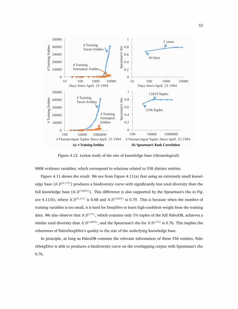
53
0
10000
20000
30000
40000
50000
10 100 1000 100000
0.2
0.4
0.6
0.8
1
10 100 1000 10000
Spea
rman
’s rh
o
Days Since April. 25 1994
60 days
2 years# Training Taxon Entities
# Training Formation Entities
Days Since April. 25 1994
0
10000
20000
30000
40000
50000
100 10000 10000000
0.2
0.4
0.6
0.8
1
100 10000 1000000
# Training Taxon Entities
# Human-input Tuples Since April. 25 1994
1296 Tuples
12839 Tuples
Spea
rman
’s rh
o
# Tr
aini
ng E
ntiti
es#
Trai
ning
Ent
ities
# Human-input Tuples Since April. 25 1994
(a) # Training Entities (b) Spearman’s Rank Correlation
# Training Formation Entities
Figure 4.12: Lesion study of the size of knowledge base (chronological).
980K evidence variables, which correspond to relations related to 55K distinct entities.
Figure 4.11 shows the result. We see from Figure 4.11(a) that using an extremely small knowl-
edge base (KB(0.1%)) produces a biodiversity curve with significantly less total diversity than the
full knowledge base (KB(100%)). This difference is also supported by the Spearman’s rho in Fig-
ure 4.11(b), where KB(0.1%) is 0.68 and KB(100%) is 0.79. This is because when the number of
training variables is too small, it is hard for DeepDive to learn high-confident weight from the training
data. We also observe that KB(1%), which contains only 1% tuples of the full PaleoDB, achieves a
similar total diversity than KB(100%), and the Spearman’s rho for KB(1%) is 0.76. This implies the
robustness of PaleoDeepDive’s quality to the size of the underlying knowledge base.
In principle, as long as PaleoDB contains the relevant information of these 556 entities, Pale-
oDeepDive is able to produces a biodiversity curve on the overlapping corpus with Spearman’s rho
0.76.

54
Chronological Replay of PaleoDB History The previous experiment uniformly samples the
knowledge base, and now we study one question that How long would it have taken for PaleoDB
volunteers to build a PaleoDB snapshot that is large enough to effectively construct PaleoDeepDive?.
To understand this question, we conduct the following experiment that “chronologically replay”
snapshots of PaleoDB.5
Each tuple in PaleoDB has a field called creation time, and we order all tuples by this field, and
create one snapshot every 30 days. This gives us a series of knowledge bases. For each knowledge
base, we use it to supervise PaleoDeepDive and report the results in Figure 4.12.
Figure 4.12(a) shows the statistics of the training data produced by this series of knowledge
bases. One see that as the number of days (since April 25 1994, the date of the first tuple) or the
number of human-input tuples grows, the number of entities appears in the training set grows.
Figure 4.12(b) shows the Spearman’s rho for each knowledge base. We find that the first non-empty
PaleoDeepDive training set happens after 60 days, when there are 1296 human-input tuples. This
achieves a Spearman’s rho of 0.65, which is much worse than the one we can get on the full PaleoDB
dump (0.79). However, with the dump on April 1996 (2 years), we can produce a diversity curve
with Spearman’s rho 0.76. This dumps only contains 12K human input tuple. The 2 year figure is
somewhat biased: the PaleoDB project did not have a large number of volunteers initially; in contrast,
by 2004 it would take only 1 month for volunteers to input a sufficient number of tuples.
4.2 TAC-KBP
We briefly describe another KBC application built with DeepDive. Different from PaleoDeepDive, this
application is built for a KBC competition called TAC-KBP, which is a public benchmark data set on
non-scientific applications.6 This allows us to compare the KBC system built with DeepDive not only
to human volunteers as we did in PaleoDeepDive, but also other state-of-the-art KBC systems. We first
describe the task of TAC-KBP, then describe the submission system we built that is the top-performing
system in TAC-KBP 2014 slot filling task among 18 teams and 65 submissions.
5One confounding effect that should be noted is that we use the same rules that we have constructed for the final system;and the extra information may have been helpful in debugging or creating these rules.
6http://www.nist.gov/tac/2014/KBP/

55
Entities Relations
Person-related Relations Organization-related Relations
alternate_namescity_of_headquarterscountry_of_headquartersdate_dissolveddate_foundedfounded_bymember_ofmembersnumber_of_employees_membersparentspolitical_religious_affiliationshareholdersstateorprovince_of_headquarterssubsidiariestop_members_employeeswebsite
agealternate_namescause_of_deathchargeschildrencountries_of_residencecountry_of_birthcountry_of_deathdate_of_birthdate_of_deathemployee_or_member_ofother_familystateorprovince_of_birthstateorprovince_of_deathstatesorprovinces_of_residence
parentsreligionschools_attendedsiblingsSpousetitlecities_of_residencecity_of_birthcity_of_deathorigin
Person
Location
Organization
Date
Cause of Death
Title
URL
Figure 4.13: The set of entities and relations in TAC-KBP competition.
4.2.1 Description of the Submission System
The slot filling task of TAC-KBP 2014 aims at extracting information from 1.8M news articles. The
target relation is similar to those appear in Freebase or Wikipedia’s information box. Figure 4.13
illustrates the set of entities and relations that a submission system needs to extract from news
articles. In totaly, there are totally 41 target relations for person entity or organization entity. We
describe system details of the two runs we submitted with DeepDive, with a focus on the lessons we
learned during the development of these systems.
Input Data Preparation The input to DeepDive is a text corpus with NLP-markups that are stored
as a database relation. The baseline system we built contains all NLP-markups produced by Stanford
CoreNLP. During our development, we find that in one system snapshot with recall=0.45, parsing-
related errors contribute to 31% of recall errors. A further analysis shows that some of these sentences
do have a correct parsing result in other parsers. Motivated by this observation, our final submission
contains the union of parsing result from three parsers, namely, Stanford CoreNLP [126], Malt
parser [143], and BBN’s SERIF [36]. Among these three parsers, we run Stanford CoreNLP and
Malt parser by ourselves, and the result of SERIF is shipped with the TAC 2014 KBP English Source
Corpus (LDC2014E13). We conduct post-processing on the result of Malt parser and SERIF to make
sure they share the same format as the output of Stanford CoreNLP. For Malt parser, we collapse

56
the dependency tree as in Stanford CoreNLP; for SERIF, we use Stanford CoreNLP to translate the
constitute parsing result into collapsed dependencies. These post-processing steps make sure we
can use exactly the same DeepDive program to process the output of all these three parsers, and
therefore, do not need to change the DeepDive program.
Feature Extraction The features we used in our submission largely follow state-of-the-art work.
Baseline features that we use include the dependency paths and word sequences between a mention
pair. For each baseline feature, we apply one or a conjunction of the following operations to generate
a new feature, including (1) replace a verb (resp. noun) with its POS or NER tag; (2) replace a verb
(resp. noun) with its WordNet synset; (3) replace a verb (resp. noun) with its WordNet hypernyms.
These are basic features that we used for a mention pair in the sentence. Another class of features that
we used involves a mention pair and a keyword (e.g., president, chair, marry, etc.) in the sentence.
Given two mentions m1, m2, and a keyword w, we create a feature that is a conjunction between
(1) (m1, w)’s feature; (2) (m2, w)’s feature; and (3) w’s lemma form. For (mi, w)’s feature, we use
the same feature extractor as we defined for a single mention pairs. The dictionary of keywords is
generated in a way described below.
Distant Supervision We follow the standard practice of distant supervision to produce positive
and negative examples. To improve upon this component, our goal is to harvest more (distantly)
labeled training examples. Therefore, our submission involves a labeling phase that is motivated by
the success of Hearst’s patterns [92] in harvesting high-quality taxonomic relations.
Our labeling effort starts from the result of standard distant supervision, which is a set of tuples
of mention pairs that are labeled as positive examples for relation R, denoted as R(m1,m2), and for
each mention pair, we have the set of features associated with it, denoted as a relation F (m1,m2, f).
Then, we pick all features f that (1) are associated with at least one mention pair in R, and (2)
appeared in the whole corpus at least twice for distinct sentences. For each feature, we manually label
it as an indicator of the relation or not. For features labeled as indicators, we only use them in the
following way–We include all mention pairs associated with this feature as newly generated positive
examples (and negative examples for other relations). One simple optimization we conducted is
that if a more general feature (e.g., the feature after substituting a noun to its POS tag) is labeled as
correct, then all features that are more specific than this feature should also be correct and do not

57
need a human label. We manually labeled 100K features in this way. Although 100K features sounds
like a large amount of features to label, we find that it only takes the author 2 days, and after getting
familiar with this task, the labeling speed could be as fast as one feature per second.
Error Analysis We conducted error analysis after the score and ground truth was released to classify
errors that our submission made into multiple categories. This error analysis is conducted on our
submission with F1=0.36 (Precision=0.54 and Recall=0.27) and focuses mainly on precision.
Out of all 509 proposed relations, 276 of them are labeled as correct, 154 wrong, 53 inexact, and
26 redundant. We mainly focus on the 154+54 wrong and inexact relations, which constitute 40
points of precision loss. Because this submission system uses a probability threshold 0.8 to propose
relations, 20 points of these errors are expected due to errors in relation extraction. In the remaining
20 points of precision loss, we find that entity linking errors contribute to 7 points of precision loss.
One common pattern is that DeepDive confuses entities which are different from the query entity but
share the same name. For example, if the query asks about “Barack Obama” and there are mentions
of “Barack Obama” and “Michelle Obama” in the same document, our system sometimes mistakenly
links a mention “Obama” referring to “Michelle Obama” to the query. Another 7 points of precision
loss are caused by normalizing answers that are of the type date, age, and title. For example, our
system did not normalize the date to the format “yyyy-mm-dd”, and these answers are labelled as
“incorrect” by the annotators. These two classes of errors require deeper understanding of entities
that appear in the corpus.

58
5. Batch Execution
But the speed was power,
and the speed was joy,
and the speed was pure beauty.
— Richard Bach, Jonathan Livingston Seagull, 1970
The thesis of this dissertation is that it is feasible to build DeepDive as a data management system
in which the user specifies what he wants to do in each phase instead of how these operations are
physically conducted. We have illustrated how DeepDive allows this declarative way of specifying a
KBC system. One question remains: Can we make the execution of DeepDive efficient and scalable?
The answer to this question is well-studied for some phases. For example, both the feature
extraction and probabilistic knowledge engineering phases rely on SQL with user-defined functions.
Because the data model of DeepDive is relational, the efficiency and scalability of these two phases
can be achieved by relying on modern (distributed) relational databases.
However, the statistical inference and learning phase requires more study. Because the operations
in this phase are not relational, making them scalable and efficient it is an active research problem
that has attracted intensive interests in recent years, as we will discuss in Chapter 7. This chapter
described two techniques that we developed for this topic. The first technique aims to scale up
one algorithm for statistical inference and learning, namely Gibbs sampling, over factor graphs
whose size exceeds tera-bytes and thus does not fit in main memory. The technical contribution is to
revisit the design of a buffer manager for statistical inference and learning algorithms. The second
technique aims to speed up statistical analytics algorithms when the problem fits in main memory.
The technical contribution is to study the system tradeoff of building an in-memory analytics system
on modern hardware. As we will see in this chapter, both techniques can lead to more than two
orders of magnitude speed up in some workloads. These techniques together allow DeepDive to
support a large range of statistical inference and learning tasks with different-sized problems and
different computational resources. Given these techniques, the user can focus more on constructing
a DeepDive program instead of worrying about how a statistical inference task could be done on
billions of random variables.

59
5.1 Scalable Gibbs Sampling
Factor graphs are the abstraction DeepDive uses for statistical inference and learning. Other than its
application in DeepDive, factor graphs also capture and unify a range of data-driven statistical tasks
in predictive analytics, and pricing and actuarial models that are used across many industries. For
example, Moody’s rating service uses Gibbs sampling and generalized linear models (GLMs) [174], as
do leading insurance actuaries [17,72]. Increasingly, more sophisticated factor graph models are used.
For example, Yahoo and Google use latent Dirichlet allocation (LDA) for topic modeling [34,122,173],
and Microsoft’s EntityCube uses Markov logic [69, 140, 163, 209]. Most inference or parameter
estimation problems for factor graphs are intractable to solve exactly [188]. To perform these tasks,
one often resorts to sampling. Arguably the most popular of these approaches, and the one on which
we focus, is Gibbs sampling [159].
Not surprisingly, frameworks that combine factor graphs and Gibbs sampling are popular and
widely used. For example, the OpenBUGS framework has been used widely since the 1980s [125].
More recent examples include PGibbs [82] and Factorie [128]. For any factor graph, given a fixed
time budget, an implementation of Gibbs sampling that produces samples at a higher throughput,
achieves higher-quality results [174]. Thus, a key technical challenge is to create an implementation
of high-throughput Gibbs samplers.
Achieving high throughput for Gibbs sampling is well studied for factor graphs that fit in main
memory, but there is a race to apply these approaches to larger amounts of data, e.g., in defense
and intelligence [136], enterprise [93], and web applications [173]. In DeepDive, the factor graph
produced for KBC can easily exceed terabytes, which does not always fit in main memory.
A key pain point of existing approaches on scalable Gibbs sampling is that for each specific model,
a scalable implementation is hand tuned, e.g., Greenplum’s MADlib [93] and Yahoo [173] implement
hand-tuned versions of LDA. High-performance implementations of Gibbs sampling often require a
tedious process of trial-and-error optimization. Further complicating an engineer’s job is that the
variety of storage backends has exploded in the last few years: traditional files, relational databases,
and HDFS-based key-value stores, like HBase or Accumulo. The lack of scalable Gibbs samplers
forces developers to revisit I/O tradeoffs for each new statistical model and each new data storage
combination. We first show that a baseline approach that picks classically optimal points in this
tradeoff space may lose almost two orders of magnitude of throughput.

60
We select three classical techniques that are used to improve query performance in database
storage managers: materialization, page-oriented layout, and buffer-replacement policy. These
techniques are simple to implement (so they may be implemented in practice), and they have stood
the test of four decades of use.1 Our study examines these techniques for a handful of popular storage
backends: main-memory based, traditional unix files, and key-value stores.
Applying these classical techniques is not as straightforward as one may think. The tradeoff
space for each technique has changed due to at least one of two new characteristics of sampling
algorithms (versus join data processing): (1) data are mutable during processing (in contrast to a
typical join algorithm), and (2) data are repeatedly accessed in an order that changes randomly across
executions, which means that we cannot precompute an ideal order. However, within any given
sampling session, the data is accessed in a fixed order. We consider the tradeoff space analytically,
and use our analysis of the tradeoff space to design a simple proof-of-concept storage manager. We
use this storage manager to validate our claimed tradeoff space in scaling Gibbs sampling.
As we show through experiments, our prototype system is competitive with even state-of-the-art,
hand-tuned approaches for factor graphs that are larger than main memory. Thus, it is possible to
achieve competitive performance using this handful of classical techniques.
5.1.0.1 Overview of Technical Contributions
The input to Gibbs sampling is a factor graph as we described in Chapter 2, which can be modeled as
a labeled bipartite graph G = (X,Y,E) where X and Y are sets of nodes and E ⊆ X × Y is a set of
edges. To obtain a sample for a single variable x, we perform three steps: (1) retrieve all neighboring
factors2 and the assignments for all variables in those factors, (2) evaluate these neighboring factors
with the retrieved assignments, and (3) aggregate the evaluation results to compute a conditional
distribution from which we select a new value for x. This operation, which we call the core operation,
is repeated for every variable in the factor graph (in a randomly selected order). We loop over the
variables many times to obtain a high-quality sample.
Since the bulk (often over 99%) of the execution time is spent in the core operation, we focus on
optimizing this operation. To this end, we identify three tradeoffs for the core operation of Gibbs
sampling: (1) materialization, (2) page-oriented layout, and (3) buffer-replacement policy. Note that
1Although sampling approaches have been integrated with data processing systems, notably the MCDB project [100], theabove techniques have not been applied to the area of high-throughput samplers.
2The set of neighboring factors are factors that connect a given variable and its Markov blanket.
61
all these three tradeoffs are among the most popular tradeoffs studied by the database community,
and our effort in adapting these general tradeoffs to more ad hoc workload is in a very similar spirit
to prior arts in database [185].
1. Materialization tradeoffs. During Gibbs sampling, we access the bipartite graph structure
many times. An obvious optimization is to materialize a portion of the graph to avoid repeated
accesses. A twist is that the value of a random variable is updated during the core operation.
Thus, materialization schemes that introduce redundancy may require many (random) writes.
This introduces a new cost in materialization schemes, and so we re-explore lazy and eager
materialization schemes, along with two co-clustering schemes [153, ch. 16]. The two co-
clustering schemes together analytically and empirically dominate both eager and lazy schemes
– but neither dominates the other. Thus, we design a simple optimizer based on statistics from
the data to choose between these two approaches.
2. Page-oriented layout. Once we have decided how to materialize or co-cluster, we are still
free to assign variables and factors to pages to minimize the number of page fetches from
the storage manager during the core operation. In cases in which the sampling is I/O bound,
minimizing the number of page fetches helps reduce this bottleneck. Since Gibbs sampling
proceeds through the variables in a random order, we want a layout that has good average-case
performance. Toward this goal, we describe a simple heuristic that outperforms a naıve random
layout by up to an order of magnitude. We then show that extending this heuristic is difficult:
assuming P 6= NP, no polynomial time algorithm has a constant-factor approximation for the
layout that minimizes page fetches during execution.
3. Buffer-Replacement Policy. A key issue, when dealing with data that is larger than available
main memory, is deciding which data to retain and which to discard from main memory, i.e.,
the buffer-replacement policy. Although the data is visited in random order, one will typically
perform many passes over the data in the same random order. Thus, after the first pass over the
data, we have a great deal of information about which pages will be selected during execution.
It turns out that this enables us to use a classical result from Belady in 1966 [26] to define a
theoretically optimal eviction strategy: evict the item that will be used latest in the future. We
implement this approach and show that it performs optimally, but that its improvement over
more traditional strategies based on MRU/LRU is only 5–10%. It also requires some non-trivial

62
implementation, and so it may be too complex for the performance gain. A technical serendipity
is that we use Belady’s result to characterize an optimal buffer-replacement strategy, which is
needed to establish our hardness result described in page-oriented layout.
We present our technical contributions in Section 5.1.1, and an empirical validation in Sec-
tion 5.1.2. We discuss related work together with other techniques in Chapter 7. We conclude in
Section 5.1.3.
5.1.1 Storage-Manager tradeoffs to Scale Gibbs Sampling
We show that Gibbs sampling essentially performs joins and updates on a view over several base
relations that represent the factor graph. Thus, we can apply classical data management techniques
(such as view materialization, page-oriented layout, and buffer-replacement policy) to achieve
scalability and high I/O efficiency.
5.1.1.1 Gibbs Sampling as a View
Given a database with a user schema and correlation schema as defined in Chapter 2, we define two
simple relations that represent the edge relation of the factor graph and the sampled possible world:
E(v, f) = (v, f)|f ∈ F, v ∈ vars(f) and A(v, a) ⊆ D× V
In Figure 2.3, E encodes the bipartite graph and each tuple in A corresponds to a possible assignment
of a label of a variable. Note that each variable is assigned a single value (so v is a key of A) and A
will be modified during Gibbs sampling.
The following view describes the input factor graph for Gibbs sampling:
Q(v, f, v′, a′)← E(v, f), E(v′, f), A(v′, a′), v 6= v′.
When running Gibbs sampling, we group Q by the first field v. Notice that the corresponding group of
tuples in Q contains all variables in the Markov blanket mb(v) along with all the factor IDs incident
to v. This is all the information we need to generate a sample. For each group, corresponding to
a variable v, we sample a new value (denoted by a) for v according to the conditional probability

63
Reads WritesStorage
from A from E ALazy |mb(v)| dv 1 O(|E|+ |A|)
V-CoC |mb(v)| 0 1 O(∑v |mb(v)|+ |A|)
F-CoC 0 dv dv O(|E|)Eager 0 0 |mb(v)| O(
∑v |mb(v)|)
Table 5.1: I/O costs for sampling one variable under different materialization strategies. For avariable v, dv is the number of factors in which v participates. Reads (resp. writes) are random reads(resp. random writes). The cost for each strategy is the total number of reads and writes.
View: Q(v, f, v’, a’) :- E(v, f), E(v, f), A(v’, a’), v ≠ v’
Base Relations: E(v, f), A(v, a)
Materialization Strategy V-CoC Materialization Strategy F-CoC
E(v, f) E(v’, f)
QV
E(v’, f) A(v’, a’)
QF
E(v, f)A(v’, a’)
⨝ ⨝
⨝ ⨝
Figure 5.1: Strategies V-CoC and F-CoC.
Pr[v|mb(v)]. The twist is that after we obtain a, we must update A before we proceed to the next
variable to be sampled. In our implementation, we proceed through the groups in a random order.3
After one pass through Q, we obtain a new possible world (represented by A). We repeat this
process to obtain multiple samples. By counting the number of occurrences of an event, e.g., a
variable taking a particular value, we can use these samples to perform marginal inference.
We describe how we optimize the data access to Q using classical data management techniques
such as view materialization and page-oriented layout. To study these tradeoffs, we implement a
simple storage system. We store E and A using slotted pages [153] and a single-pool buffer manager.4

64
5.1.1.2 Materializing the Factor Graph
The view Q involves a three-way join. All join operators perform an index nested-loop join (see
Figure 5.1) with a small twist: the join keys are also record IDs, hence we do not need to perform an
actual index look-up to find the appropriate page. We examine materialization strategies to improve
the performance of these joins.5
Materialization can reduce the number of random reads. However, a key twist is that the base
relation A is updated after we examine each group. Thus, if we replicate A we could incur many
random writes. We study this tradeoff by comparing four different materialization strategies in terms
of random read/write costs and space requirements of different strategies described as follows.
• Lazy: we only materialize base tables. This strategy incurs the most random reads for on-the-fly
joins, but the fewest random writes.
• V-CoC: we co-cluster on the variable side
QV (v, f, v′)← E(v, f), E(v′, f), v 6= v′
Compared to the lazy strategy, this strategy eliminates random reads on E and retains a single
copy of A.
• F-CoC: we co-cluster on the factor side
QF (f, v′, a)← E(v′, f), A(v′, a)
Compared to the lazy strategy, this strategy eliminates random reads on A at the cost of more
random writes to update A within QF .
• Eager: we eagerly materialize Q. This strategy eliminates all random reads at the cost of high
random writes during the core operation.
3Our strategy is independent of the order. The order, however, empirically does change the convergence rate, and it isfuture work to understand the tradeoff of order and convergence.
4We use variable and factor IDs as record IDs, and so can look up the column v or f in both E and A using one randomaccess (similar to RID lists [153, ch. 16]).
5Since we run many iterations of Gibbs sampling, the construction cost of materialized views is often smaller than the costof running Gibbs sampling in all strategies. (In all of our experiments, the construction cost is less than 25% of the total runtime.)

65
Figure 5.1 illustrates the two co-clustering strategies.
From Table 5.1, we see that V-CoC dominates Lazy and F-CoC dominates Eager in terms of random
accesses (Assuming each factor contains at least two variables, |mb(v)| ≥ 2dv). Our experiments
confirm these analytic models (see Section 5.1.2.3). Therefore, our system selects between V-CoC
and F-CoC. To determine which approach to use, our system selects the materialization strategy with
the smallest random I/O cost according to our cost model.
5.1.1.3 Page-oriented Layout
With either V-CoC or F-CoC, Q is an index nested-loop join between one relation clustered on
variables and another relation clustered on factors. How the data are organized into pages impacts
I/O efficiency in any environment.
We formalize the problem of page-oriented layout for Gibbs sampling as follows, GLAYOUT.
The input to the problem is a tuple (V, F,E, µ, S, P ) where (V, F,E) define a factor graph; that is,
V = v1, . . . , vN is a set of variables, F = f1, . . . , fM is the set of factors, and E = (v, f) | v ∈
vars(f) defines the edge relation. The order µ is a total order on the variables, V , which captures
the fact that at each iteration of Gibbs sampling, one scans the variables in V in a random order, and
S the page size (i.e., the maximum number of variables a page can store), and P the set of pages.
Any solution for GLAYOUT is a tuple (α, β, π) where α : V 7→ P (resp. β : F 7→ P ) map variables
(resp. factors) to pages. The order π = (e1, . . . , eL) defines the order of edges that the algorithm
visits. That is, given a fixed variable visit order µ = (v1, . . . , vN ), we only consider tuple orders π that
respect µ; we denote this set of orders as Π(µ).6
As we will see, it is possible in Gibbs sampling to construct an optimal page eviction strategy. For
the moment, to simplify our presentation, we assume that there are only two buffer pages: one for
variables and one for factors. We return to this point later. Then any ordering π = (e1, . . . , eL) would
incur an I/O cost (for fetching factors from disk):
cost(π, β) = 1 +
L∑i=2
I [β(ei.f) 6= β(ei−1.f)]
The goal is to find an ordering π ∈ Π(µ) and mapping β that minimizes the above I/O cost.
6 Π(µ) = π = (e1, . . . , eL) | ∀i, j.1 ≤ i ≤ j ≤ L, ei.v µ ej .v, where x µ y indicates that x precedes y in µ.

66
Algorithm We use the following simple heuristic to construct (α, β, π) ordering F : we sort the
factors in F in dictionary order by µ, that is, by the position of the earliest variable that occurs in a
given factor. We then greedily pack F -tuples onto disk pages in this order. We show empirically that
this layout has one order of magnitude improvement over randomly ordering and paging tuples.
We find that extending this heuristic for better performance is theoretically challenging:
Proposition 5.1. Assuming P 6=NP, an algorithm does not exist that runs in polynomial time to find the
optimal solution to GLAYOUT. More strongly, assuming P 6=NP, no polynomial time algorithm can even
guarantee a constant approximation factor for cost.
We prove this proposition in the Appendix A.1 by encoding the multi-cut partition problem [14].
Under slightly more strict complexity assumptions (about randomized complexity classes), it also
follows that getting a good layout on average is computationally difficult.
Multi-page Buffer We return to the issue of more than two buffer pages. Since variables are
accessed sequentially, MRU is optimal for the variable pages. One could worry that the additional
number of buffer pages could be used intelligently to lower the cost. We show that we are able to
reduce the multiple-page buffer case to the two-page case (and so an approximation result similar to
Proposition 5.1); intuitively, given the instance generated for the two-buffer case, we include extra
factors whose role in the reduction is to ensure that any optimal buffering strategy essentially incurs
I/O only on the sequence of buffer pages that it would in the two-buffer case. Our proof examines
the set of pages in Belady’s [26] optimal strategy, which we describe in the next section.
5.1.1.4 Buffer-Replacement Policy
When a data set does not fit in main memory, we must choose which page to evict from main memory.
A key twist here is that we will be going over the same data set many times. After the first pass, we
know the full reference sequence for the remainder of the execution. This enables us to use a classical
result from Belady in the 1960s [26] to define a theoretically optimal eviction strategy: evict the item
that will be used latest in the future.
Recall that we scan variables in sequential order, so MRU is optimal for those pages. However,
the factor pages require a bit more care. On the first pass of the data, we store the entire reference
sequence of factors in a file, i.e., sequence fi1 , fi2 , . . . , lists each factor. For each reference, we then

67
Systems LR CRF LDA Storage ParallelismElementary X X X Multiple Multi-thread
Factorie X X X RAM Single-threadPGibbs X X X RAM Multi-thread
OpenBUGS X X RAM Single-threadMADlib X Database Multi-thread
Table 5.2: Key features of each system that implements Gibbs sampling. OpenBUGS and MADlib donot support skip-chain CRFs. MADlib supports LR but not a full Bayesian (sampling) treatment; itssupport for LDA is via specialized UDFs.
do a pass over this log to compute when each factor is used next in the sequence. At the end of the
first scan, we have a log that consists of pairs of factor IDs and when each factor appears next. The
resulting file may be several GB in size. However, during the subsequent passes, we only need the
head of this log in main memory. We use this information to maintain, for each frame in the buffer
manager, when that frame will be used next.
In our experiments, we evaluate under what situations this optimal strategy is worth the extra
overhead. We find that the optimal strategy is close to the standard LRU in terms of run time–even if
we allow the potentially unfair advantage of holding the entire reference sequence in main memory.
In both cases, the number of page faults is roughly 5%–10% smaller using the optimal approach.
However, we found that simple schemes based on MRU/LRU are essentially optimal in two tasks
(LR and CRF in the next section), and in the third task (LDA in the next section) the variables share
factors that are far apart, and so even the optimal strategy cannot mitigate all random I/O.
5.1.2 Experiments
We validate that (1) our system is able to scale to factor graphs that are larger than main memory,
and (2) for inference on factor graphs that are larger than main memory, we achieve throughput that
is competitive with specialized approaches. We then validate the details of our technical claims about
materialization, page-oriented layout, and buffer-replacement policy that we described.
5.1.2.1 Experimental Setup
We run experiments on three popular statistical models: 1) logistic regression (LR), 2) skip-chain
conditional random field [182] (CRF), and 3) latent Dirichlet allocation (LDA). We use LR and CRF
for text chunking, and LDA for topic modeling. We select LR because it can be solved exactly and so

68
ModelsBench (1x) Perf (1,000x) Scale (100,000x)
|V | |F | Size |V | |F | Size |V | |F | SizeLR 47K 47K 2MB 47M 47M 2GB 5B 5B 0.19TB
CRF 47K 94K 3MB 47M 94M 3GB 5B 9B 0.3TBLDA 0.4M 12K 10M 0.4B 10M 9GB 39B 0.2B 0.9TB
Table 5.3: Data sets sizes. We omit the 10x, 100x, and 10,000x cases from this table.
can be used as a simple benchmark. We select CRF as it is widely used in text-related applications and
inference is often performed with Gibbs sampling, and LDA as it is intuitively the most challenging
model that is supported by all systems in our experiments.
Data Sets To compare the quality and efficiency with other systems, we use public data sets that we
call Bench. We run LR and CRF on CoNLL7 and LDA on AP.8 For scalability experiments and tradeoff
efficiency experiments, we scale up Bench from 1x to 100,000x by adding more documents which are
randomly selected from a one-day web crawl (5M documents, 400GB). We call the 1,000x data set
Perf and the 100,000x data set Scale. Table 5.3 shows the number of variables, factors, and size.
Metrics We use two metrics to measure the quality: (1) the F1 score of the final result for data
sets with ground truth (when ground truth is available) and (2) the squared loss [194] between the
marginal probabilities that are the output of each sampling system and a gold standard on each data
set (when there is no ground truth). For LR, we compute the gold standard using exact inference.
For CRF and LDA, it is intractable to compute the exact distribution; and the standard approach is to
use the results from Gibbs sampling after running many iterations beyond convergence [194]. In
particular, we get an approximate gold standard for both CRF and LDA on Bench by running Gibbs
sampling for 10M iterations. For efficiency, we measure the throughput as the number of samples
produced by a system per second.
Competitor Systems We compare our system with four state-of-the-art Gibbs sampling systems:
(1) PGibbs on GraphLab [82], (2) Factorie [128], and (3) OpenBUGS [125], which are main memory
systems, and MADlib [93], a scalable in-database implementation of LDA. PGibbs and MADlib9 are
implemented using C++, OpenBUGS is implemented using Pascal and C, and Factorie is implemented
7http://www.cnts.ua.ac.be/conll2000/chunking/8http://www.cs.princeton.edu/~blei/lda-c/9http://doc.madlib.net/v0.3/group__grp__plda.html

69
Setting Name Page Size Buffer SizeSp/Sb 4KB 40KBLp/Sb 4MB 40MBSp/Lb 4KB 4GBLp/Lb 4MB 4GB
Lp/MAXb 4MB 40GB
Table 5.4: Different configuration settings of Elementary. Sp (resp. Lp) means small (resp. large) pagesize; Sb (resp. Lb) means small (resp. large) buffer-size.
using Java. We use Greenplum 4.2.1.0 for MADlib. The key features of each system are shown in
Table 5.2. For each model (i.e., LR, CRF, and LDA), all systems take the same factor graph as their
input. We modify each system to output squared loss after each iteration, and we do not count this
time as part of the execution time.
Details of our Prototype We call our prototype system Elementary, and compare three variants
of our system by plugging in different storage backends: EleMM, EleFILE, and EleHBASE. We use
main memory, traditional unix files, and HBase,10 respectively, for these three variants. EleMM is
used to compare with other main memory systems. EleFILE and EleHBASE use different secondary
storage and are used to validate scalability and I/O tradeoffs.
Our system is implemented using C++ and bypasses the OS disk-page cache to support its own
buffer manager. We compile all C++ code using GCC 4.7.2 and all Java code using Java 1.7u4. All
experiments are run on a RHEL6.1 workstation with two 2.67GHz Intel Xeon CPUs (12 cores, 24
hyper-threaded), 128GB of RAM, and 12×2TB RAID0 drives. All data and temporary files are stored
on a RAID, and all software is installed on a separate disk. We use the latest HBase-0.94.1 on a single
machine11 and follow best practices to tune HBase.12
We use various page-size/buffer-size combinations, as shown in Table 5.4. These configuration
settings correspond to small/large page sizes and small/large buffer sizes. We explored more settings
but the high-level conclusions are similar to these four settings so we omit those results. The
Lp/MAXb setting is used for end-to-end experiments.
10http://hbase.apache.org11Our system can use HBase on multiple machines to get even higher scalability. We only discuss the one-machine case to
be fair to other systems.12http://hbase.apache.org/book/performance.html

70
# thread = 1 # threads = 20LR CRF LDA LR CRF LDA
EleMM 24 18 12 12x 9x 6xEleFILE 34 24 33 9x 6x 4x
EleHBASE 101 70 92 9x 7x 4xPGibbs 38 42 CRASH 9x 5x CRASHMADLib N/A N/A 17 N/A N/A 8xFactorie 95 120 6 N/A N/A N/A
OpenBUGS 150 N/A CRASH N/A N/A N/A
Table 5.5: The time in seconds (speedup for 20-threads case) needed to achieve squared loss below0.01 for Bench data set. N/A means that the task is not supported.
5.1.2.2 End-to-end Efficiency and Scalability
We validate that our system achieves state-of-the-art quality by demonstrating that it converges to
the gold-standard probability distribution on each task. We then compare our system’s efficiency and
scalability with that of our competitors.
Quality We validate that our system converges to the gold-standard probability distribution on
several tasks. We run all systems on Bench using the configuration Lp/MAXb. We take a snapshot
after each system produces a sample; we output the squared loss and F1 score of that snapshot.
Table 5.5 shows the time that each system needs to converge to a solution with a squared loss less
than 0.01. We chose 0.01 since a smaller loss does not improve the F1 score, i.e., when the loss is
less than 0.01, LR converges to F1=0.79 and CRF to F1=0.81, which are the gold-standard values
for these tasks. This validates that all systems achieve the same quality, and thus a more interesting
question is to understand the rate at which they achieve the quality.
Efficiency To understand the rate at which a system achieves the gold-standard quality, we run
PGibbs, MADlib, Factorie, and OpenBUGS and measure when they are within 0.01 of the optimal
loss. If a system can take advantage of multi-threading, we also run it with 20 threads and report the
speedup factor compared with one thread. We chose our materialization strategy to be consistent
with what is hard coded in state-of-the-art competitors, i.e., V-CoC for LR and CRF, and F-CoC for
LDA. Table 5.5 shows the results.
When there is one thread and all the data fit in main memory, we observe that all systems
converge to gold-standard probability distribution within roughly comparable times. This is likely due
to the fact that main memory Gibbs sampling uses a set of well-known techniques, which are widely

71
implemented. There are, however, some minor differences in runtime. On LR and CRF, EleMM has
comparable efficiency to PGibbs, but is slightly faster. After reviewing PGibbs’ code, we believe the
efficiency difference (<2x) is caused by the performance overhead of PGibbs explicitly representing
factor functions as a table. For LR and CRF, EleMM is 4–10x faster than Factorie, and we believe
that this is because Factorie is written in Java (not C++). OpenBUGS is more than one order of
magnitude slower than EleMM. This difference in OpenBUGS is due to the inefficiency in how it
records the samples of each variable. PGibbs requires explicit enumeration of all outcomes for each
factor, and so the input size to PGibbs is exponential in the size of the largest factor. As LDA involves
factors with hundreds or more variables, we could not run LDA on PGibbs. OpenBUGS crashed on
LDA while compiling the model and data with the error message “illegal memory read.” Elementary
with secondary storage backends has similar performance trends, but is overall 2–5x slower than
EleMM, due to the overhead of I/O.
For 20-thread cases, we observe speedups for all multi-threading systems. EleFILE and EleHBASE
gets smaller speedups compared with EleMM because of the overhead of I/O requests. PGibbs also
gets slightly smaller speedups than EleMM, and we believe that this marginal difference is caused by
the overhead of MPI, which is used by PGibbs.
Scalability We validate that our system can scale to larger data sets by using secondary storage
backends. We run all systems on data sets scaling from 1x (Bench) to 100,000x (Scale) using one
thread and Lp/MAXb. We let each system run for 24 hours and stop it afterwards. Figure 5.2 shows
the results for LR and LDA. We also run a baseline system, Baseline, that uses the file system as
storage and disables all of our optimizations (lazy materialization, and no buffer management).
Not surprisingly, only systems that use secondary storage backends, i.e., EleFILE, EleHBASE, and
MADlib (only for LDA), scale to the largest data sets; in contrast, main memory systems crash or
thrash at scaling factors of 10x or more. As the core operation is scan based, it also not surprising
that each system scales up almost linearly (if it is able to run).
However, the performance of the various approaches can be quite different. The Baseline system is
three orders of magnitude slower than EleMM (it does not finish the first iteration within 24 hours on
the 100x scale factor). This shows that buffer management is crucial to implementing an I/O-efficient
Gibbs sampler. Due to higher I/O overheads, EleHBASE is 3x slower than EleFILE.
MADlib uses PostgreSQL as the storage backend, and is 2x faster than EleFILE. However, MADlib

72
0.00
001
0.00
01
0.00
1
0.010.
1110
1x10
x10
0x1,
000x
10,0
00x
Throughput (#samples/second)
Dat
a se
t siz
e
0.00
0001
0.00
001
0.00
01
0.00
1
0.010.
1110
1x10
x10
0x1,
000x
10,0
00x
Dat
a se
t siz
e
Elle
MM
Elle
FILE
Elle
HBA
SE
Fact
orie
Pgib
bs
Ope
nBU
Gs
MA
Dlib
Bas
elin
e
Idea
l slo
pe fo
r lin
ear
scal
e-up
Doe
s no
t fin
ish
in 1
0 ho
urs
Doe
s no
t fin
ish
in 1
0 ho
urs
Idea
l slo
pe fo
r lin
ear
scal
e-up
(a)
LR(b
) LD
A
Figu
re5.
2:Sc
alab
ility
ofD
iffe
rent
Syst
ems.
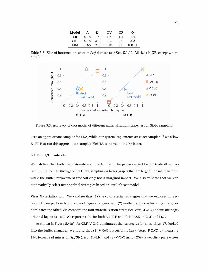
73
Model A E QV QF QLR 0.18 1.4 1.4 1.4 1.4
CRF 0.18 2.0 3.2 2.0 3.2LDA 1.66 9.0 100T+ 9.0 100T+
Table 5.6: Size of intermediate state in Perf dataset (see Sec. 5.1.1). All sizes in GB, except wherenoted.
Normalized estimated throughput
Nor
mal
ized
thr
ough
put
0
0.2
0.4
0.6
0.8
1
0 0.2 0.4 0.6 0.8 10
0.2
0.4
0.6
0.8
1
0 0.2 0.4 0.6 0.8 1
LAZY
EAGER
V-CoC
F-CoCIdealcost model
Idealcost model
(a) CRF (b) LDA
Figure 5.3: Accuracy of cost model of different materialization strategies for Gibbs sampling.
uses an approximate sampler for LDA, while our system implements an exact sampler. If we allow
EleFILE to run this approximate sampler, EleFILE is between 10-20% faster.
5.1.2.3 I/O tradeoffs
We validate that both the materialization tradeoff and the page-oriented layout tradeoff in Sec-
tion 5.1.1 affect the throughput of Gibbs sampling on factor graphs that are larger than main memory,
while the buffer-replacement tradeoff only has a marginal impact. We also validate that we can
automatically select near-optimal strategies based on our I/O cost model.
View Materialization We validate that (1) the co-clustering strategies that we explored in Sec-
tion 5.1.1 outperform both Lazy and Eager strategies, and (2) neither of the co-clustering strategies
dominates the other. We compare the four materialization strategies; our GLAYOUT heuristic page-
oriented layout is used. We report results for both EleFILE and EleHBASE on CRF and LDA.
As shown in Figure 5.4(a), for CRF, V-CoC dominates other strategies for all settings. We looked
into the buffer manager; we found that (1) V-CoC outperforms Lazy (resp. F-CoC) by incurring
75% fewer read misses on Sp/Sb (resp. Sp/Lb); and (2) V-CoC incurs 20% fewer dirty page writes

74
0
0.2
0.4
0.6
0.81
CR
F (E
lleFI
LE)
Normalized throughput
0
0.2
0.4
0.6
0.81
LDA
(El
leFI
LE)
0
0.2
0.4
0.6
0.81
CR
F (E
lleH
BASE
)
0
0.2
0.4
0.6
0.81
LDA
(El
leH
BASE
)
LAZY
EAG
ERV-
CoC
F-C
oCD
oes
not f
inis
h in
1 h
our
Doe
s no
t fin
ish
in 1
hou
r
0
0.2
0.4
0.6
0.81
0
0.2
0.4
0.6
0.81
0
0.2
0.4
0.6
0.81
Gre
edy
Shuf
fle
0
0.2
0.4
0.6
0.81
Doe
s no
t fin
ish
in 1
hou
r
0
0.2
0.4
0.6
0.81
0
0.2
0.4
0.6
0.81
0
0.2
0.4
0.6
0.81
Sp/S
bLp
/Sb
Sp/L
bLp
/Lb
Sp/S
bLp
/Sb
Sp/L
bLp
/Lb
Sp/S
bLp
/Sb
Sp/L
bLp
/Lb
Sp/S
bLp
/Sb
Sp/L
bLp
/Lb
Page
-siz
e/bu
ffer
-siz
e se
ttin
gs
(a)
Mat
eria
lizat
ion
(b)
Page
-ori
ente
d la
yout
(c)
Buf
fer
repl
acem
ent
polic
y0
0.2
0.4
0.6
0.81
Opt
imal
LRU
Rand
om
Figu
re5.
4:I/
Otr
adeo
ffs
onPe
rfda
tase
t.R
ecal
ltha
tSp
(res
p.Lp
)m
eans
smal
l(re
sp.
larg
e)pa
gesi
ze;S
b(r
esp.
Lb)
mea
nssm
all(
resp
.la
rge)
buffe
rsi
ze.
See
Tabl
e5.
4fo
rth
eex
act
defin
itio
nsof
page
and
buff
ersi
zese
ttin
gs

75
than Eager. The situation, however, is reversed in LDA. Here, F-CoC dominates, as both V-CoC and
Eager fail to run LDA as they would require 100TB+ of disk space for materialization. Thus, neither
co-clustering strategy dominates the other, but one always dominates both Eager and Lazy. The same
observation holds for both EleFILE and EleHBASE.
A key difference between these tasks is that the number of variables in most factors in LDA is much
larger (can be larger than 1,000) than LR and CRF (fewer than 3). Thus, some pre-materialization
strategies are expensive in LDA. On the other hand, for LR and CRF, the time needed to look up
factors is the bottleneck (which is optimized by V-CoC).
We then validate that one can automatically select between different materialization strategies by
using the cost model shown in Table 5.1. For each model and materialization strategy, we estimated
the throughput as the inverse of the estimated total amount of I/O. For each materialization strategy,
we plot its estimated and actual throughput. Figure 5.3 shows the results for EleFILE (Sp/Lb). We
can see that the throughput decreases when the estimated throughput decreases. Based on this cost
model, we can select the near-optimal materialization strategy.
Page-oriented Layout We validate that our heuristic ordering strategy can improve sampling
throughput over a random ordering. We focus on the F-CoC materialization strategy here because
the V-CoC setting has similar results. We compare two page-oriented layout strategies: (1) Shuffle,
in which we randomly shuffle the factor table, and (2) Greedy, which use our greedy heuristic to
layout the factor table. As shown in Figure 5.4(b), Greedy dominates Shuffle on all data sets in
both settings. For CRF, the heuristic can achieve two orders of magnitude of speedup. We found
that for Sp/Lb, heuristic ordering incurs two orders of magnitude fewer page faults than random
ordering. These results show that the tradeoff in page-oriented layout impacts the throughput of
Gibbs sampling on factor graphs that do not fit in memory.
Buffer-Replacement Policy We validate that the optimal buffer-replacement strategy can only
achieve a marginal improvement of sampling throughput over LRU. We compare three settings: (1)
Optimal, which uses the optimal caching strategy on tables with random access, (2) LRU, which
uses LRU on tables with random access; and (3) Random, which uses a random replacement policy.
We use MRU on tables with sequential scan. We use V-CoC for LR and CRF, F-CoC for LDA, and
Greedy for all page-oriented layouts because they are the optimal strategies for these tasks. As

76
shown in Figure 5.4(c), Optimal achieves 10% higher throughput than Random for CRF, and 5%
higher throughput than LRU for LDA. For CRF, the access pattern of factors is much like a sequence
scan, and therefore LRU is near-optimal. As Optimal requires non-trivial implementation and is not
implemented in existing data processing systems, an engineer may opt against implementing it in a
production system.
Discussion On this small set of popular tasks, experiments demonstrate that our prototype can
achieve competitive (and sometimes better) throughput and scalability than state-of-the-art systems
for Gibbs sampling from factor graphs that are larger than main memory. What is interesting to
us about this result is that we used a set of generic optimizations inspired by classical database
techniques. Of course, in any given problem, there may be problem-specific optimizations that can
dramatically improve throughput. For example, in higher-level languages like MCDB or Factorie, there
may be additional optimization opportunities. Our goal, however, is not to exhaustively enumerate
such optimizations; instead, we view the value of our work as articulating a handful of tradeoffs that
may be used to improve the throughput of either specialized or generic systems for Gibbs sampling
from factor graphs. These tradeoffs have not been systematically studied in previous work. Also,
our techniques are orthogonal to optimizations that choose between various sampling methods to
improve runtime performance, e.g., Wang et al. [189]. A second orthogonal direction is distributing
the data to many machines; such an approach would allow us to achieve higher scalability and
performance. We believe that the optimizations that we describe are still useful in the distributed
setting. However, there are new tradeoffs that may need to be considered, e.g., communication and
replication tradeoffs are obvious areas to explore.
5.1.3 Conclusion to Scalable Gibbs Sampling
We studied how to run Gibbs sampling over factor graphs, the abstraction DeepDive used for statistical
inference and learning phase. Our goal is to make a highly scalable Gibbs sampler. All other things
being equal, a Gibbs sampler that produces samples with higher throughput allows us to obtain
high quality more quickly. Thus, the central technical challenge is how to create a high-throughput
sampler. In contrast to previous approaches that optimize sampling by proposing new algorithms,
we examined whether or not traditional database optimization techniques could be used to improve
the core operation of Gibbs sampling. In particular, we study the impact of a handful of classical

77
data management tradeoffs on the throughput of Gibbs sampling on factor graphs that are larger
than main memory. Our work articulates a handful of tradeoffs that may be used to improve the
throughput of such systems, including materialization, page-oriented layout, and buffer-management
tradeoffs. After analytically examining the tradeoff space for each technique, we described novel
materialization strategies and a greedy page-oriented layout strategy.
Our experimental study found that our techniques allowed us to achieve up to two orders of
magnitude improvement in throughput over classical techniques. Using a classical result due to
Belady, we implemented the optimal page-replacement strategy, but found empirically that it offered
only modest improvement over traditional techniques. Overall, we saw that by optimizing for only
these classical tradeoffs, we were able to construct a prototype system that achieves competitive (and
sometimes much better) throughput than prior Gibbs sampling systems for factor graphs.
5.2 Efficient In-memory Statistical Analytics
We now focus on the task of running statistical inference and learning when the data fit in main
memory. In this section, we extend our scope boarder to not only consider factor graph, but also a
more general class of problem called statistical analytics, that contains more (sometimes simpler)
models such as linear regression, support vector machines, or logistic regression. As we will show in
Section 5.2.4, this study allows us to apply what we learned from statistical analytics to factor graph.
Statistical analytics is one of the hottest topics in data-management research and practice. Today,
even small organizations have access to machines with large main memories (via Amazon’s EC2)
or for purchase at $5/GB. As a result, there has been a flurry of activity to support main-memory
analytics in both industry (Google Brain [116], Impala, and Pivotal) and research (GraphLab [123],
and MLlib [176]). Each of these systems picks one design point in a larger tradeoff space. The goal
of this section is to define and explore this space. We find that today’s research and industrial systems
under-utilize modern hardware for analytics—sometimes by two orders of magnitude. We hope that
our study identifies some useful design points for the next generation of such main-memory analytics
systems.
Throughout, we use the term statistical analytics to refer to those tasks that can be solved by
first-order methods–a class of iterative algorithms that use gradient information; these methods are
the core algorithm in systems such as MLlib, GraphLab, and Google Brain. Our study examines

78
analytics on commodity multi-socket, multi-core, non-uniform memory access (NUMA) machines,
which are the de facto standard machine configuration and thus a natural target for an in-depth
study. Moreover, our experience with several enterprise companies suggests that, after appropriate
preprocessing, a large class of enterprise analytics problems fit into the main memory of a single,
modern machine. While this architecture has been recently studied for traditional SQL-analytics
systems [51], it has not been studied for statistical analytics systems.
Statistical analytics systems are different from traditional SQL-analytics systems. In comparison
to traditional SQL-analytics, the underlying methods are intrinsically robust to error. On the other
hand, traditional statistical theory does not consider which operations can be efficiently executed.
This leads to a fundamental tradeoff between statistical efficiency (how many steps are needed until
convergence) and hardware efficiency (how efficiently those steps can be carried out).
To describe such tradeoffs more precisely, we describe the setup of the analytics tasks that we
consider in this section. The input data is a matrix in RN×d and the goal is to find a vector x ∈ Rd
that minimizes some (convex) loss function, say the logistic loss or the hinge loss (SVM). Typically,
one makes several complete passes over the data while updating the model; following conventions,
we call each such pass an epoch. There may be some communication at the end of the epoch, e.g., in
bulk-synchronous parallel systems such as Spark [201]. We identify three tradeoffs that have not
been explored in the literature: (1) access methods for the data, (2) model replication, and (3) data
replication. Current systems have picked one point in this space; we explain each space and discover
points that have not been previously considered. Using these new points, we can perform 100×
faster than previously explored points in the tradeoff space for several popular tasks.
Access Methods Analytics systems access (and store) data in either row-major or column-major
order. For example, systems that use stochastic gradient descent methods (SGD) access the data
row-wise; examples include MADlib [93] in Impala and Pivotal, Google Brain [116], and MLlib in
Spark [176]; and stochastic coordinate descent methods (SCD) access the data column-wise; examples
include GraphLab [123], Shogun [175], and Thetis [177]. These methods have essentially identical
statistical efficiency, but their wall-clock performance can be radically different due to hardware
efficiency. However, this tradeoff has not been systematically studied. We introduce a storage
abstraction that captures the access patterns of popular statistical analytics tasks and a prototype
called DimmWitted. In particular, we identify three access methods that are used in popular analytics

79
tasks, including standard supervised machine learning models such as SVMs, logistic regression, and
least squares; and more advanced methods such as neural networks and Gibbs sampling on factor
graphs. For different access methods for the same problem, we find that the time to converge to a
given loss can differ by up to 100×.
We also find that no access method dominates all others, so an engine designer may want to
include both access methods. To show that it may be possible to support both methods in a single
engine, we develop a simple cost model to choose among these access methods. We describe a simple
cost model that selects a nearly optimal point in our data sets, models, and different machines.
Data and Model Replication We study two sets of tradeoffs: the level of granularity, and the
mechanism by which mutable state and immutable data are shared in analytics tasks. We describe
the tradeoffs we explore in both (1) mutable state sharing, which we informally call model replication,
and (2) data replication.
(1) Model Replication During execution, there is some state that the task mutates (typically an
update to the model). We call this state, which may be shared among one or more processors, a
model replica. We consider three different granularities at which to share model replicas:
• The PerCPU approach treats a NUMA machine as a distributed system in which every core is
treated as an individual machine, e.g., in bulk-synchronous models such as MLlib on Spark
or event-driven systems such as GraphLab. These approaches are the classical shared-nothing
and event-driven architectures, respectively. In PerCPU, the part of the model that is updated
by each core is only visible to that core until the end of an epoch. This method is efficient
and scalable from a hardware perspective, but it is less statistically efficient, as there is only
coarse-grained communication between cores.
• The PerMachine approach acts as if each processor has uniform access to memory. This approach
is taken in Hogwild! [141] and Google Downpour [66]. In this method, the hardware takes
care of the coherence of the shared state. The PerMachine method is statistically efficient due to
high communication rates, but it may cause contention in the hardware, which may lead to
suboptimal running times.

80
• A natural hybrid is PerNode, in which a node is a NUMA node that contains multiple CPU cores;
this method uses the fact that PerCPU communication through the last-level cache (LLC) is
dramatically faster than communication through remote main memory. This method is novel;
for some models, PerNode can be an order of magnitude faster.
Because model replicas are mutable, a key question is how often should we synchronize model replicas?
We find that it is beneficial to synchronize the models as much as possible—so long as we do not
impede throughput to data in main memory. A natural idea, then, is to use PerMachine sharing,
in which the hardware is responsible for synchronizing the replicas. However, this decision can
be suboptimal, as the cache-coherence protocol may stall a processor to preserve coherence, but
this information may not be worth the cost of a stall from a statistical efficiency perspective. We
find that the PerNode method, coupled with a simple technique to batch writes across sockets, can
dramatically reduce communication and processor stalls. The PerNode method can result in an over
10× runtime improvement. This technique depends on the fact that we do not need to maintain the
model consistently: we are effectively delaying some updates to reduce the total number of updates
across sockets (which lead to processor stalls).
(2) Data Replication The data for analytics is immutable, so there are no synchronization issues
for data replication. The classical approach is to partition the data to take advantage of higher
aggregate memory bandwidth. However, each partition may contain skewed data, which may slow
convergence. Thus, an alternate approach is to replicate the data fully (say, per NUMA node). In this
approach, each node accesses that node’s data in a different order, which means that the replicas
provide non-redundant statistical information; in turn, this reduces the variance of the estimates
based on the data in each replicate. We find that for some tasks, fully replicating the data four ways
can converge to the same loss almost 4× faster than the sharding strategy.
Summary of Contributions Westudy the three tradeoffs listed above for main-memory statistical
analytics systems. These tradeoffs are not intended to be an exhaustive set of optimizations, but
they demonstrate our main conceptual point: treating NUMA machines as distributed systems or SMP
is suboptimal for statistical analytics. We design a storage manager, DimmWitted, that shows it is
possible to exploit these ideas on real data sets. Finally, we evaluate our techniques on multiple real
datasets, models, and architectures.

81
N
d
(a) Memory Model for DimmWitted
Data A Model x
Machine
Node 1
L3 Cache
RAM
Core1
(d) NUMA Architecture(c) Access Methods
Row-wise Col.-wise Col.-to-row
Read set of dataWrite set of model
(b) Pseudocode of SGD
Procedure:m <-- initial modelwhile not converge
foreach row z in A:m <-- m – α grad(z, m)
test convergence
Input: Data matrix A, stepsize αGradient function grad.
Output: Model m.
Epoch
L1/L2
d
L1/L2
Core2
Node 2
L3 Cache
RAM
Core3
L1/L2 L1/L2
Core4
Figure 5.5: Illustration of (a) DimmWitted’s Memory Model, (b) Pseudocode for SGD, (c) DifferentStatistical Methods in DimmWitted and Their Access Patterns, and (d) NUMA Architecture.
5.2.1 Background
In this section, we describe the memory model for DimmWitted, which provides a unified memory
model to implement popular analytics methods. Then, we recall some basic properties of modern
NUMA architectures.
Data for Analytics The data for an analytics task is a pair (A, x), which we call the data and the
model, respectively. For concreteness, we consider a matrix A ∈ RN×d. In machine learning parlance,
each row is called an example. Thus, N is often the number of examples and d is often called the
dimension of the model. There is also a model, typically a vector x ∈ Rd. The distinction is that
the data A is read-only, while the model vector, x, will be updated during execution. From the
perspective of this section, the important distinction we make is that data is an immutable matrix,
while the model (or portions of it) are mutable data.

82
First-Order Methods for Analytic Algorithms DimmWitted considers a class of popular algorithms
called first-order methods. Such algorithms make several passes over the data; we refer to each such
pass as an epoch. A popular example algorithm is stochastic gradient descent (SGD), which is widely
used by web-companies, e.g., Google Brain and VowPal Wabbit [4], and in enterprise systems such
as Pivotal, Oracle, and Impala. Pseudocode for this method is shown in Figure 5.5(b). During each
epoch, SGD reads a single example z; it uses the current value of the model and z to estimate the
derivative; and it then updates the model vector with this estimate. It reads each example in this
loop. After each epoch, these methods test convergence (usually by computing or estimating the
norm of the gradient); this computation requires a scan over the complete dataset.
5.2.1.1 Memory Models for Analytics
We design DimmWitted’s memory model to capture the trend in recent high-performance sampling
and statistical methods. There are two aspects to this memory model: the coherence level and the
storage layout.
Coherence Level Classically, memory systems are coherent: reads and writes are executed atomi-
cally. For analytics systems, we say that a memory model is coherent if reads and writes of the entire
model vector are atomic. That is, access to the model is enforced by a critical section. However, many
modern analytics algorithms are designed for an incoherent memory model. The Hogwild! method
showed that one can run such a method in parallel without locking but still provably converge. The
Hogwild! memory model relies on the fact that writes of individual components are atomic, but it
does not require that the entire vector be updated atomically. However, atomicity at the level of the
cacheline is provided by essentially all modern processors. Empirically, these results allow one to
forgo costly locking (and coherence) protocols. Similar algorithms have been proposed for other pop-
ular methods, including Gibbs sampling [103,173], stochastic coordinate descent (SCD) [158,175],
and linear systems solvers [177]. This technique was applied by Dean et al. [66] to solve convex
optimization problems with billions of elements in a model. This memory model is distinct from the
classical, fully coherent database execution [153].
The DimmWitted prototype allows us to specify that a region of memory is coherent or not. This
region of memory may be shared by one or more processors. If the memory is only shared per thread,

83
Algorithm Access Method ImplementationStochastic Gradient Descent Row-wise MADlib, Spark, Hogwild!
Stochastic Coordinate DescentColumn-wise
GraphLab, Shogun, ThetisColumn-to-row
Table 5.7: Algorithms and Their Access Methods.
then we can simulate a shared-nothing execution. If the memory is shared per machine, we can
simulate Hogwild!.
Access Methods We identify three distinct access paths used by modern analytics systems, which
we call row-wise, column-wise, and column-to-row. They are graphically illustrated in Figure 5.5(c).
Our prototype supports all three access methods. All of our methods perform several epochs, that is,
passes over the data. However, the algorithm may iterate over the data row-wise or column-wise.
• In row-wise access, the system scans each row of the table and applies a function that takes
that row, applies a function to it, and then updates the model. This method may write to all
components of the model. Popular methods that use this access method include stochastic
gradient descent, gradient descent, and higher-order methods (such as l-BFGS).
• In column-wise access, the system scans each column j of the table. This method reads just the j
component of the model. The write set of the method is typically a single component of the
model. This method is used by stochastic coordinate descent.
• In column-to-row access, the system iterates conceptually over the columns. This method is
typically applied to sparse matrices. When iterating on column j, it will read all rows in which
column j is non-zero. This method also updates a single component of the model. This method
is used by non-linear support vector machines in GraphLab and is the de facto approach for
Gibbs sampling.
DimmWitted is free to iterate over rows or columns in essentially any order (although typically some
randomness in the ordering is desired). Table 5.7 classifies popular implementations by their access
method.

84
Name (abbrv.) #Node #Cores/Node RAM/Node (GB) CPU Clock (GHz) LLC (MB)local2 (l2) 2 6 32 2.6 12local4 (l4) 4 10 64 2.0 24local8 (l8) 8 8 128 2.6 24ec2.1 (e1) 2 8 122 2.6 20ec2.2 (e2) 2 8 30 2.6 20
Table 5.8: Summary of Machines. Tested with STREAM [30], local2 has intra-node bandwidth 6GB/sand inter-node QPI 12 GB/s.
Machine
Data A
Model x
Optimizer
Execution Plan
……
Data Replica Worker Model Replica
Read Update
Figure 5.6: Illustration of DimmWitted’s engine.
5.2.1.2 Architecture of NUMA Machines
We briefly describe the architecture of a modern NUMA machine. As illustrated in Figure 5.5(d), a
NUMA machine contains multiple NUMA nodes. Each node has multiple cores and processor caches,
including the L3 cache. Each node is directly connected to a region of DRAM. NUMA nodes are
connected to each other by buses on the main board; in our case, this connection is the Intel Quick
Path Interconnects (QPIs), which has a bandwidth as high as 25.6GB/s. To access DRAM regions of
other NUMA nodes, data is transferred across NUMA nodes using the QPI. These NUMA architectures
are cache coherent, and the coherency actions use the QPI. Table 5.8 describes the configuration
of each machine that we use in this section. Machines controlled by us have names with the prefix
“local”; the other machines are Amazon EC2 configurations.

85
Tradeoff Strategies Existing Systems
Access MethodsRow-wise SP, HW
Column-wise GLColumn-to-row GL
Model ReplicationPer Core GL, SPPer Node
Per Machine HW
Data ReplicationSharding GL, SP, HW
Full Replication
Table 5.9: A Summary of DimmWitted’s Tradeoffs and Existing Systems (GraphLab (GL), Hogwild!(HW), Spark (SP)).
5.2.2 The DimmWitted Engine
We describe the tradeoff space that DimmWitted’s optimizer considers, namely (1) access method
selection, (2) model replication, and (3) data replication. To help understand the statistical-versus-
hardware tradeoff space, we present some experimental results in a Tradeoffs paragraph within each
subsection. We describe implementation details for DimmWitted in Appendix A.2.
5.2.2.1 System Overview
We describe analytics tasks in DimmWitted and the execution model of DimmWitted.
System Input For each analytics task that we study, we assume that the user provides data A ∈
RN×d and an initial model that is a vector of length d. In addition, for each access method listed
above, there is a function of an appropriate type that solves the same underlying model. For example,
we provide both a row- and column-wise way of solving a support vector machine. Each method
takes two arguments; the first is a pointer to a model.
• frow captures the the row-wise access method, and its second argument is the index of a single
row.
• fcol captures the column-wise access method, and its second argument is the index of a single
column.
• fctr captures the column-to-row access method, and its second argument is a pair of one column
index and a set of row indexes. These rows correspond to the non-zero entries in a data matrix
for a single column.13
13Define S(j) = i : aij 6= 0. For a column j, the input to fctr is a pair (j, S(j)).

86
Algorithm Read Write (Dense) Write (Sparse)Row-wise
∑i ni dN
∑i ni
Column-wise∑i ni d d
Column-to-row∑i n
2i d d
Table 5.10: Per Epoch Execution Cost of Row- and Column-wise Access. The Write column is for asingle model replica. Given a dataset A ∈ RN×d, let ni be the number of non-zero elements ai.
Each of the functions modifies the model to which they receive a pointer in place. However, in our
study, frow can modify the whole model, while fcol and fctr only modify a single variable of the
model. We call the above tuple of functions a model specification. Note that a model specification
contains either fcol or fctr but typically not both.
Execution Given a model specification, our goal is to generate an execution plan. An execution
plan, schematically illustrated in Figure 5.6, specifies three things for each CPU core in the machine:
(1) a subset of the data matrix to operate on, (2) a replica of the model to update, and (3) the access
method used to update the model. We call the set of replicas of data and models locality groups,
as the replicas are described physically; i.e., they correspond to regions of memory that are local
to particular NUMA nodes, and one or more workers may be mapped to each locality group. The
data assigned to distinct locality groups may overlap. We use DimmWitted’s engine to explore three
tradeoffs:
(1) Access methods, in which we can select between either the row or column method to access
the data.
(2) Model replication, in which we choose how to create and assign replicas of the model to each
worker. When a worker needs to read or write the model, it will read or write the model replica
that it is assigned.
(3) Data replication, in which we choose a subset of data tuples for each worker. The replicas may
be overlapping, disjoint, or some combination.
Table 5.9 summarizes the tradeoff space. In each section, we illustrate the tradeoff along two axes,
namely (1) the statistical efficiency, i.e., the number of epochs it takes to converge, and (2) hardware
efficiency, the time that each method takes to finish a single epoch.

87
0.01
0.1
1
10
0.1 1 10
Tim
e/Ep
och
(sec
onds
)
Cost Ratio
Row-wise
Column-wise
(a) Number of Epochs to Converge (b) Time for Each Epoch
1
10
100
SVM1 SVM2 LP1 LP2
# Ep
och
Models and Data Sets
Column-wiseRow-wise
Figure 5.7: Illustration of the Method Selection Tradeoff. (a) These four datasets are RCV1, Reuters,Amazon, and Google, respectively. (b) The “cost ratio” is defined as the ratio of costs estimated forrow-wise and column-wise methods: (1 +α)
∑i ni/(
∑i n
2i +αd), where ni is the number of non-zero
elements of ith row of A and α is the cost ratio between writing and reads. We set α = 10 to plot thisgraph.
5.2.2.2 Access Method Selection
In this section, we examine each access method: row-wise, column-wise, and column-to-row. We find
that the execution time of an access method depends more on hardware efficiency than on statistical
efficiency.
Tradeoffs We consider the two tradeoffs that we use for a simple cost model (Table 5.10). Let ni
be the number of non-zeros in row i; when we store the data as sparse vectors/matrices in CSR
format, the number of reads in a row-wise access method is∑Ni=1 ni. Since each example is likely to
be written back in a dense write, we perform dN writes per epoch. Our cost model combines these
two costs linearly with a factor α that accounts for writes being more expensive, on average, because
of contention. The factor α is estimated at installation time by measuring on a small set of datasets.
The parameter α is in 4 to 12 and grows with the number of sockets; e.g., for local2, α ≈ 4, and for
local8, α ≈ 12. Thus, α may increase in the future.
Statistical Efficiency. We observe that each access method has comparable statistical efficiency.
To illustrate this, we run all methods on all of our datasets and report the number of epochs that one
method converges to a given error to the optimal loss, and Figure 5.7(a) shows the result on four
datasets with 10% error. We see that the gap in the number of epochs across different methods is
small (always within 50% of each other).

88
Hardware Efficiency. Different access methods can change the time per epoch by up to a factor
of 10×, and there is a cross-over point. To see this, we run both methods on a series of synthetic
datasets where we control the number of non-zero elements per row by subsampling each row on
the Music dataset (see Section 5.2.3 for more details). For each subsampled dataset, we plot the
cost ratio on the x-axis, and we plot their actual running time per epoch in Figure 5.7(b). We see
a cross-over point on the time used per epoch: when the cost ratio is small, row-wise outperforms
column-wise by 6×, as the column-wise method reads more data; on the other hand, when the ratio is
large, the column-wise method outperforms the row-wise method by 3×, as the column-wise method
has lower write contention. We observe similar cross-over points on our other datasets.
Cost-based Optimizer DimmWitted estimates the execution time of different access methods using
the number of bytes that each method reads and writes in one epoch, as shown in Table 5.10. For
writes, it is slightly more complex: for models such as SVM, each gradient step in row-wise access
only updates the coordinates where the input vector contains non-zero elements. We call this scenario
a sparse update; otherwise, it is a dense update.
DimmWitted needs to estimate the ratio of the cost of reads to writes. To do this, it runs a simple
benchmark dataset. We find that, for all the eight datasets, five statistical models, and five machines
that we use in the experiments, the cost model is robust to this parameter: as long as writes are 4×
to 100× more expensive than reading, the cost model makes the correct decision between row-wise
and column-wise access.
5.2.2.3 Model Replication
In DimmWitted, we consider three model replication strategies. The first two strategies, namely
PerCPU and PerMachine, are similar to traditional shared-nothing and shared-memory architecture,
respectively. We also consider a hybrid strategy, PerNode, designed for NUMA machines.
Granularity of Model Replication The difference between the three model replication strategies is
the granularity of replicating a model. We first describe PerCPU and PerMachine and their relationship
with other existing systems (Table 5.9). We then describe PerNode, a simple, novel hybrid strategy
that we designed to leverage the structure of NUMA machines.

89
1. PerCPU. In the PerCPU strategy, each core maintains a mutable state, and these states are
combined to form a new version of the model (typically at the end of each epoch). This is
essentially a shared-nothing architecture; it is implemented in Impala, Pivotal, and Hadoop-
based frameworks. PerCPU is popularly implemented by state-of-the-art statistical analytics
frameworks such as Bismarck, Spark, and GraphLab. There are subtle variations to this
approach: in Bismarck’s implementation, each worker processes a partition of the data, and its
model is averaged at the end of each epoch; Spark implements a minibatch-based approach
in which parallel workers calculate the gradient based on examples, and then gradients are
aggregated by a single thread to update the final model; GraphLab implements an event-based
approach where each different task is dynamically scheduled to satisfy the given consistency
requirement. In DimmWitted, we implement PerCPU in a way that is similar to Bismarck,
where each worker has its own model replica, and each worker is responsible for updating its
replica.14 As we will show in the experiment section, DimmWitted’s implementation is 3-100×
faster than either GraphLab and Spark. Both systems have additional sources of overhead that
DimmWitted does not, e.g., for fault tolerance in Spark and a distributed environment in both.
We are not making an argument about the relative merits of these features in applications, only
that they would obscure the tradeoffs that we study in this section.
2. PerMachine. In the PerMachine strategy, there is a single model replica that all workers update
during execution. PerMachine is implemented in Hogwild! and Google’s Downpour. Hogwild!
implements a lock-free protocol, which forces the hardware to deal with coherence. Although
different writers may overwrite each other and readers may have dirty reads, Niu et al. [141]
prove that Hogwild! converges.
3. PerNode. The PerNode strategy is a hybrid of PerCPU and PerMachine. In PerNode, each NUMA
node has a single model replica that is shared among all cores on that node.
Model Synchronization Deciding how often the replicas synchronize is key to the design. In
Hadoop-based and Bismarck-based models, they synchronize at the end of each epoch. This is a
shared-nothing approach that works well in user-defined aggregations. However, we consider finer
14We implemented MLlib’s minibatch in DimmWitted. We find that the Hogwild!-like implementation always dominatesthe minibatch implementation. DimmWitted’s column-wise implementation for PerMachine is similar to GraphLab, with theonly difference that DimmWitted does not schedule the task in an event-driven way.

90
1
10
100
1000
10000
0.01 0.1 1
PerCore#
Epoc
h
Error to Optimal Loss
(a) Number of Epochs to Converge
PerNode
PerMachine
(b) Time for Each Epoch
0.1
1
10
PerMachine PerNode PerCPU
Tim
e/Ep
och
(sec
ond)
Model Replication Strategies
Figure 5.8: Illustration of Model Replication Tradeoff in DimmWitted.
granularities of sharing. In DimmWitted, we chose to have one thread that periodically reads models
on all other cores, averages their results, and updates each replica.
One key question for model synchronization is how frequently should the model be synchronized?
Intuitively, we might expect that more frequent synchronization will lower the throughput; on the
other hand, the more frequently we synchronize, the fewer number of iterations we might need to
converge. However, in DimmWitted, we find that the optimal choice is to communicate as frequently
as possible. The intuition is that the QPI has staggering bandwidth (25GB/s) compared to the
small amount of data we are shipping (megabytes). As a result, in DimmWitted, we implement an
asynchronous version of the model averaging protocol: a separate thread averages models, with the
effect of batching many writes together across the cores into one write, reducing the number of stalls.
Tradeoffs We observe that PerNode is more hardware efficient, as it takes less time to execute an
epoch than PerMachine; PerMachine might use fewer number of epochs to converge than PerNode.
Statistical Efficiency. We observe that PerMachine usually takes fewer epochs to converge to the
same loss compared to PerNode, and PerNode uses fewer number of epochs than PerCPU. To illustrate
this observation, Figure 5.8(a) shows the number of epochs that each strategy requires to converge
to a given loss for SVM (RCV1). We see that PerMachine always uses the least number of epochs
to converge to a given loss: intuitively, the single model replica has more information at each step,
which means that there is less redundant work. We observe similar phenomena when comparing
PerCPU and PerNode.

91
1
10
100
1000
10000
100000
1% 10% 100%
Sharding
FullReplication
(a) Number of Epochs to Converge (b) Time for Each Epoch
0.0001
0.001
0.01
local2 local4 local8
Sharding
FullReplication
Tim
e/Ep
och
(sec
onds
)
# Ep
och
Error to Optimal Loss Different Machines
Figure 5.9: Illustration of Data Replication Tradeoff in DimmWitted.
Hardware Efficiency. We observe that PerNode uses much less time to execute an epoch than
PerMachine. To illustrate the difference in the time that each model replication strategy uses to
finish one epoch, we show in Figure 5.8(b) the execution time of three strategies on SVM (RCV1).
We see that PerNode is 23× faster than PerMachine and that PerCPU is 1.5× faster than PerNode.
PerNode takes advantage of the locality provided by the NUMA architecture. Using PMUs, we find
that PerMachine incurs 11× more cross-node DRAM requests than PerNode.
Rule of Thumb For SGD-based models, PerNode usually gives optimal results, while for SCD-based
models, PerMachine does. Intuitively, this is caused by the fact that SGD has a denser update pattern
than SCD, so, PerMachine suffers from hardware efficiency.
5.2.2.4 Data Replication
In DimmWitted, each worker processes a subset of data and then updates its model replica. To assign
a subset of data to each worker, we consider two strategies.
1. Sharding. Sharding is a popular strategy implemented in systems such as Hogwild!, Spark, and
Bismarck, in which the dataset is partitioned, and each worker only works on its partition of
data. When there is a single model replica, Sharding avoids wasted computation, as each tuple
is processed once per epoch. However, when there are multiple model replicas, Sharding might
increase the variance of the estimate we form on each node, lowering the statistical efficiency.
In DimmWitted, we implement Sharding by randomly partitioning the rows (resp. columns) of

92
a data matrix for the row-wise (resp. column-wise) access method. In column-to-row access,
we also replicate other rows that are needed.
2. FullReplication. A simple alternative to Sharding is FullReplication, in which we replicate the
whole dataset many times (PerCPU or PerNode). In PerNode, each NUMA node will have a
full copy of the data. Each node accesses its data in a different order, which means that the
replicas provide non-redundant statistical information. Statistically, there are two benefits of
FullReplication: (1) averaging different estimates from each node has a lower variance, and (2)
the estimate at each node has lower variance than in the Sharding case, as each node’s estimate
is based on the whole data. From a hardware efficiency perspective, reads are more frequent
from local NUMA memory in PerNode than in PerMachine. The PerNode approach dominates
the PerCPU approach, as reads from the same node go to the same NUMA memory. Thus, we
do not consider PerCPU replication from this point on.
Tradeoffs Not surprisingly, we observe that FullReplication takes more time for each epoch than
Sharding. However, we also observe that FullReplication uses fewer epochs than Sharding, especially
to achieve low error. We illustrate these two observations by showing the result of running SVM on
Reuters using PerNode in Figure 5.9.
Statistical Efficiency. FullReplication uses fewer epochs, especially to low-error tolerance. Fig-
ure 5.9(a) shows the number of epochs that each strategy takes to converge to a given loss. We see
that, for within 1% of the loss, FullReplication uses 10× fewer epochs on a two-node machine. This
is because each model replica sees more data than Sharding, and therefore has a better estimate.
Because of this difference in the number of epochs, FullReplication is 5× faster in wall-clock time than
Sharding to converge to 1% loss. However, we also observe that, at high-error regions, FullReplication
uses more epochs than Sharding and causes a comparable execution time to a given loss.
Hardware Efficiency. Figure 5.9(b) shows the time for each epoch across different machines with
different numbers of nodes. Because we are using the PerNode strategy, which is the optimal choice
for this dataset, the more nodes a machine has, the slower FullReplication is for each epoch. The
slow-down is roughly consistent with the number of nodes on each machine. This is not surprising
because each epoch of FullReplication processes more data than Sharding.

93
Model Dataset #Row #Col. NNZ Size (Sparse) Size (Dense) Sparse
SVM, LR, LS
RCV1 781K 47K 60M 914MB 275GB XReuters 8K 18K 93K 1.4MB 1.2GB XMusic 515K 91 46M 701MB 0.4GBForest 581K 54 30M 490MB 0.2GB
LPAmazon 926K 335K 2M 28MB >1TB XGoogle 2M 2M 3M 25MB >1TB X
QPAmazon 1M 1M 7M 104MB >1TB XGoogle 2M 2M 10M 152MB >1TB X
Gibbs Paleo 69M 30M 108M 2GB >1TB XNN MNIST 120M 800K 120M 2GB >1TB X
Table 5.11: Dataset Statistics. NNZ refers to the Number of Non-zero elements. The # columns isequal to the number of variables in the model.
5.2.3 Experiments
We validate that exploiting the tradeoff space that we described enables DimmWitted’s orders of
magnitude speedup over state-of-the-art competitor systems. We also validate that each tradeoff
discussed in this section affects the performance of DimmWitted.
5.2.3.1 Experiment Setup
Datasets and Statistical Models We validate the performance and quality of DimmWitted on a
diverse set of statistical models and datasets. For statistical models, we choose five models that
are among the most popular models used in statistical analytics: (1) Support Vector Machine
(SVM), (2) Logistic Regression (LR), (3) Least Squares Regression (LS), (4) Linear Programming
(LP), and (5) Quadratic Programming (QP). For each model, we choose datasets with different
characteristics, including size, sparsity, and under- or over-determination. For SVM, LR, and LS, we
choose four datasets: Reuters15, RCV116, Music17, and Forest.18 Reuters and RCV1 are datasets for
text classification that are sparse and underdetermined. Music and Forest are standard benchmark
datasets that are dense and overdetermined. For QP and LR, we consider a social-network application,
i.e., network analysis, and use two datasets from Amazon’s customer data and Google’s Google+
social networks.19 Table 5.11 shows the dataset statistics.
15archive.ics.uci.edu/ml/datasets/Reuters-21578+Text+Categorization+Collection16about.reuters.com/researchandstandards/corpus/17archive.ics.uci.edu/ml/datasets/YearPredictionMSD18archive.ics.uci.edu/ml/datasets/Covertype19snap.stanford.edu/data/

94
Dat
aset
Wit
hin
1%of
the
Opt
imal
Loss
Wit
hin
50%
ofth
eO
ptim
alLo
ssG
raph
Lab
Gra
phC
hiM
Llib
Hog
wild
!D
WG
raph
Lab
Gra
phC
hiM
Llib
Hog
wild
!D
W
SVM
Reu
ters
58.9
56.7
15.5
0.1
0.1
13.6
11.2
0.6
0.01
0.01
RC
V1
>30
0.0
>30
0.0
>300
61.4
26.8
>300.0
>300.0
58.
00.
710.
17M
usic
>30
0.0
>30
0.0
156
33.3
223
.731.2
27.1
7.7
0.17
0.14
Fore
st16.2
15.8
2.7
00.
230.
011.
91.4
0.15
0.03
0.01
LRR
eute
rs36.3
34.2
19.2
0.1
0.1
13.2
12.5
1.2
0.03
0.03
RC
V1
>30
0.0
>30
0.0
>300.0
38.7
19.8
>300.0
>300.0
68.
00.
820.
20M
usic
>30
0.0
>30
0.0
>300.0
35.7
28.6
30.2
28.9
8.9
0.56
0.34
Fore
st29
.228
.73.7
40.
290.
032.
32.
50.
17
0.02
0.01
LSR
eute
rs13
2.9
121.2
92.5
4.1
3.2
16.3
16.7
1.9
0.17
0.09
RC
V1
>30
0.0
>30
0.0
>300
27.5
10.5
>300.0
>300.0
32.
01.
300.
40M
usic
>30
0.0
>30
0.0
221
40.1
25.8
>300.0
>300.0
11.
20.
780.
52Fo
rest
25.5
26.5
1.0
10.
330.
022.
72.
90.
15
0.04
0.01
LPA
maz
on2.
72.
4>
120.0
>120.0
0.94
2.7
2.1
120.0
1.86
0.94
Goo
gle
13.4
11.9
>120.0
>120.0
12.5
62.
32.
0120.0
3.04
2.02
QP
Am
azon
6.8
5.7
>120.0
>120.0
1.8
6.8
5.7
>120.0
>120.0
01.
50G
oogl
e12
.410
.1>
120.0
>120.0
4.3
9.9
8.3
>120.0
>120.0
03.
70
Tabl
e5.
12:
End-
to-E
ndC
ompa
riso
n(t
ime
inse
cond
s).
The
colu
mn
DW
refe
rsto
Dim
mW
itte
d.W
eta
ke5
runs
onlo
cal2
and
repo
rtth
eav
erag
e(s
tand
ard
devi
atio
nfo
ral
lnum
bers<
5%of
the
mea
n).
Entr
ies
wit
h>
indi
cate
ati
meo
ut.

95
Metrics We measure the quality and performance of DimmWitted and other competitors. To
measure the quality, we follow prior art and use the loss function for all functions. For end-to-end
performance, we measure the wall-clock time it takes for each system to converge to a loss that is
within 100%, 50%, 10%, and 1% of the optimal loss.20 When measuring the wall-clock time, we do
not count the time used for data loading and result outputting for all systems. We also use other
measurements to understand the details of the tradeoff space, including (1) local LLC request, (2)
remote LLC request, and (3) local DRAM request. We use Intel Performance Monitoring Units (PMUs)
and follow the manual21 to conduct these experiments.
Experiment Setting We compare DimmWitted with four competitor systems: GraphLab [123],
GraphChi [113], MLlib [176] over Spark [201], and Hogwild! [141]. GraphLab is a distributed graph
processing system that supports a large range of statistical models. GraphChi is similar to GraphLab
but with a focus on multi-core machines with secondary storage. MLlib is a package of machine
learning algorithms implemented over Spark, an in-memory implementation of the MapReduce
framework. Hogwild! is an in-memory lock-free framework for statistical analytics. We find that all
four systems pick some points in the tradeoff space that we considered in DimmWitted. In GraphLab
and GraphChi, all models are implemented using stochastic coordinate descent (column-wise access);
in MLlib and Hogwild!, SVM and LR are implemented using stochastic gradient descent (row-wise
access). We use implementations that are provided by the original developers whenever possible.
For models without code provided by the developers, we only change the corresponding gradient
function.22 For GraphChi, if the corresponding model is implemented in GraphLab but not GraphChi,
we follow GraphLab’s implementation.
We run experiments on a variety of architectures. These machines differ in a range of config-
urations, including the number of NUMA nodes, the size of last-level cache (LLC), and memory
bandwidth. See Table 5.8 for a summary of these machines. DimmWitted, Hogwild!, GraphLab, and
GraphChi are implemented using C++, and MLlib/Spark is implemented using Scala. We tune both
GraphLab and MLlib according to their best practice guidelines.23 For both GraphLab, GraphChi,
20We obtain the optimal loss by running all systems for one hour and choosing the lowest.21software.intel.com/en-us/articles/performance-monitoring-unit-guidelines22For sparse models, we change the dense vector data structure in MLlib to a sparse vector, which only improves its
performance.23 MLlib:spark.incubator.apache.org/docs/0.6.0/tuning.html;
GraphLab: graphlab.org/tutorials-2/fine-tuning-graphlab-performance/;For GraphChi, we tune the memory buffer size to ensure all data fit in memory and that there are no disk I/Os.

96
110
100
1000
1%10
%10
0%
110100
1000
1%10
%10
0%
0.11
10100
1000
1%10%
100%
0.11
10100
1%10%
100%
0.010.
11
10
1%10
%10
0%
0.010.1110
1%10%
100%
0.11
10100
1%10
%10
0%
0.11
10100
1%10
%10
0%
SVM
(R
CV
1)
Erro
r to
Opt
imal
Los
s
SVM
(M
usic
)LP
(A
maz
on)
LP (
Goo
gle)
PerN
odePe
rMac
hine
(a) Access Method Sel.
Time (seconds)
Row
-wis
e
Col
umn-
wis
e
PerC
ore
Time (seconds)
(b) Model Replication
Figu
re5.
10:
Trad
eoff
sin
Dim
mW
itte
d.M
issi
ngpo
ints
tim
eout
in12
0se
cond
s.

97
and MLlib, we try different ways of increasing locality on NUMA machines, including trying to use
numactl and implementing our own RDD for MLlib. Systems are compiled with g++ 4.7.2 (-O3),
Java 1.7, or Scala 2.9.
5.2.3.2 End-to-End Comparison
We validate that DimmWitted outperforms competitor systems in terms of end-to-end performance
and quality. Note that both MLlib and GraphLab have extra overhead for fault tolerance, distributing
work, and task scheduling. Our comparison between DimmWitted and these competitors is intended
only to demonstrate that existing work for statistical analytics has not obviated the tradeoffs that we
study here.
Protocol For each system, we grid search their statistical parameters, including step size (100.0,
10.0, ..., 0.0001) and mini-batch size for MLlib (1%, 10%, 50%, 100%); we always report the best
configuration, which is essentially the same for each system. We measure the time it takes for each
system to find a solution that is within 1%, 10%, and 50% of the optimal loss. Table 5.12 shows the
results for 1% and 50%; the results for 10% are similar. We report end-to-end numbers from local2,
which has two nodes and 24 logical cores, as GraphLab does not run on machines with more than 64
logical cores. Table 5.14 shows the DimmWitted’s choice of point in the tradeoff space on local2.
As shown in Table 5.12, DimmWitted always converges to the given loss in less time than the
other competitors. On SVM and LR, DimmWitted could be up to 10× faster than Hogwild!, and more
than two orders of magnitude faster than GraphLab and Spark. The difference between DimmWitted
and Hogwild! is greater for LP and QP, where DimmWitted outperforms Hogwild! by more than
two orders of magnitude. On LP and QP, DimmWitted is also up to 3× faster than GraphLab and
GraphChi, and two orders of magnitude faster than MLlib.
Tradeoff Choices We dive more deeply into these numbers to substantiate our claim that there
are some points in the tradeoff space that are not used by GraphLab, GraphChi, Hogwild!, and
MLlib. Each tradeoff selected by our system is shown in Table 5.14. For example, GraphLab and
GraphChi uses column-wise access for all models, while MLlib and Hogwild! use row-wise access for
all models and allow only PerMachine model replication. These special points work well for some
but not all models. For example, for LP and QP, GraphLab and GraphChi are only 3× slower than

98
DimmWitted, which chooses column-wise and PerMachine. This factor of 3 is to be expected, as
GraphLab also allows distributed access and so has additional overhead. However there are other
points: for SVM and LR, DimmWitted outperforms GraphLab and GraphChi, because the column-wise
algorithm implemented by GraphLab and GraphChi is not as efficient as row-wise on the same dataset.
DimmWitted outperforms Hogwild! because DimmWitted takes advantage of model replication, while
Hogwild! incurs 11× more cross-node DRAM requests than DimmWitted; in contrast, DimmWitted
incurs 11× more local DRAM requests than Hogwild! does.
For SVM, LR, and LS, we find that DimmWitted outperforms MLlib, primarily due to being
located at a different point in the tradeoff space. In particular, MLlib uses batch-gradient-descent
with a PerCPU implementation, while DimmWitted uses stochastic gradient and PerNode. We find
that, for the Forest dataset, DimmWitted takes 60× fewer number of epochs to converge to 1%
loss than MLlib. For each epoch, DimmWitted is 4× faster. These two factors contribute to the
240× speed-up of DimmWitted over MLlib on the Forest dataset (1% loss). MLlib has overhead for
scheduling, so we break down the time that MLlibuses for scheduling and computation. We find that,
for Forest, out of the total 2.7 seconds of execution, MLlib uses 1.8 seconds for computation and 0.9
seconds for scheduling. We also implemented a batch-gradient-descent and PerCPU implementation
inside DimmWitted to remove these and C++ versus Scala differences. The 60× difference in the
number of epochs until convergence still holds, and our implementation is only 3× faster than MLlib.
This implies that the main difference between DimmWitted and MLlib is the point in the tradeoff
space—not low-level implementation differences.
For LP and QP, DimmWitted outperforms MLlib and Hogwild! because the row-wise access
method implemented by these systems is not as efficient as column-wise access on the same data
set. GraphLab does have column-wise access, so DimmWitted outperforms GraphLab and GraphChi
because DimmWitted finishes each epoch up to 3× faster, primarily due to low-level issues. This
supports our claims that the tradeoff space is interesting for analytic engines and that no one system
has implemented all of them.
Throughput We compare the throughput of different systems for an extremely simple task: parallel
sums. Our implementation of parallel sum follows our implementation of other statistical models
(with a trivial update function), and uses all cores on a single machine. Table 5.13 shows the through-
put on all systems on different models on one dataset. We see from Table 5.13 that DimmWitted

99
SVM LR LS LP QP Parallel(RCV1) (RCV1) (RCV1) (Google) (Google) Sum
GraphLab 0.2 0.2 0.2 0.2 0.1 0.9GraphChi 0.3 0.3 0.2 0.2 0.2 1
MLlib 0.2 0.2 0.2 0.1 0.02 0.3Hogwild! 1.3 1.4 1.3 0.3 0.2 13
DimmWitted 5.1 5.2 5.2 0.7 1.3 21
Table 5.13: Comparison of Throughput (GB/seconds) of Different Systems on local2.
Model and Dataset Access Method Model Replication Data Replication
SVM, LR, LSReuters
Row-wise PerNode FullReplicationRCV1Music
LP, QPAmazon
Column-wise PerMachine FullReplicationGoogle
Table 5.14: Plans that DimmWitted Chooses for Each Dataset on Machine local2.
achieves the highest throughput of all the systems. For parallel sum, DimmWitted is 1.6× faster
than Hogwild!, and we find that DimmWitted incurs 8× fewer LLC cache misses than Hogwild!.
Compared with Hogwild!, in which all threads write to a single copy of the sum result, DimmWitted
maintains one single copy of the sum result per NUMA node, so the workers on one NUMA node do
not invalidate the cache on another NUMA node. When running on only a single thread, DimmWitted
has the same implementation as Hogwild!. Compared with GraphLab and GraphChi, DimmWitted
is 20× faster, likely due to the overhead of GraphLab and GraphChi dynamically scheduling tasks
and/or maintaining the graph structure. To compare DimmWitted with MLlib, which is written
in Scala, we implemented a Scala version, which is 3× slower than C++; this suggests that the
overhead is not just due to the language. If we do not count the time that MLlibuses for scheduling
and only count the time of computation, we find that DimmWitted is 15× faster than MLlib.
5.2.3.3 Tradeoffs of DimmWitted
We validate that all the tradeoffs described in this section have an impact on the efficiency of
DimmWitted. We report on a more modern architecture, local4 with four NUMA sockets, in this
section. We describe how the results change with different architectures.
Access Method Selection We validate that different access methods have different performance,
and that no single access method dominates the others. We run DimmWitted on all statistical models

100
0.01
0.1
1
10
100
0.01
0.1
1
10
100
Rat
io o
f Exe
cutio
n Ti
me
per
Epoc
h (ro
w-w
ise/
col-w
ise)
(a) SVM (RCV1) (b) LP (Amazon)
[e1] [e2] [l2] [l4] [l8]8x2 8x2 6x2 10x4 8x8
#Cores/Socket # Sockets [Machine Name]
[e1] [e2] [l2] [l4] [l8]8x2 8x2 6x2 10x4 8x8
Figure 5.11: Ratio of Execution Time per Epoch (row-wise/column-wise) on Different Architectures.A number larger than 1 means that row-wise is slower. l2 means local2, e1 means ec2.1, etc.
and compare two strategies, row-wise and column-wise. In each experiment, we force DimmWitted to
use the corresponding access method, but report the best point for the other tradeoffs. Figure 5.10(a)
shows the results as we measure the time it takes to achieve each loss. The more stringent loss
requirements (1%) are on the left-hand side. The horizontal line segments in the graph indicate that
a model may reach, say, 50% as quickly (in epochs) as it reaches 100%.
We see from Figure 5.10(a) that the difference between row-wise and column-to-row access could
be more than 100× for different models. For SVM on RCV1, row-wise access converges at least 4×
faster to 10% loss and at least 10× faster to 100% loss. We observe similar phenomena for Music;
compared with RCV1, column-to-row access converges to 50% loss and 100% loss at a 10× slower
rate. With such datasets, the column-to-row access simply requires more reads and writes. This
supports the folk wisdom that gradient methods are preferable to coordinate descent methods. On
the other hand, for LP, column-wise access dominates: row-wise access does not converge to 1%
loss within the timeout period for either Amazon or Google. Column-wise access converges at least
10-100× faster than row-wise access to 1% loss. We observe that LR is similar to SVM and QP is
similar to LP. Thus, no access method dominates all the others.
The cost of writing and reading are different and is captured by a parameter that we called
α in Section 5.2.2.2. We describe the impact of this factor on the relative performance of row-
and column-wise strategies. Figure 5.11 shows the ratio of the time that each strategy uses (row-
wise/column-wise) for SVM (RCV1) and LP (Amazon). We see that, as the number of sockets on a

101
machine increases, the ratio of execution time increases, which means that row-wise becomes slower
relative to column-wise, i.e., with increasing α. As the write cost captures the cost of a hardware-
resolved conflict, we see that this constant is likely to grow. Thus, if next-generation architectures
increase in the number of sockets, the cost parameter α and consequently the importance of this
tradeoff are likely to grow.
Cost-based Optimizer We observed that, for all datasets, our cost-based optimizer selects row-
wise access for SVM, LR, and LS, and column-wise access for LP and QP. These choices are consistent
with what we observed in Figure 5.10.
Model Replication We validate that there is no single strategy for model replication that dominates
the others. We force DimmWitted to run strategies in PerMachine, PerNode, and PerCPU and choose
other tradeoffs by choosing the plan that achieves the best result. Figure 5.10(b) shows the results.
We see from Figure 5.10(b) that the gap between PerMachine and PerNode could be up to 100×.
We first observe that PerNode dominates PerCPU on all datasets. For SVM on RCV1, PerNode
converges 10× faster than PerCPU to 50% loss, and for other models and datasets, we observe
a similar phenomenon. This is due to the low statistical efficiency of PerCPU, as we discussed in
Section 5.2.2.3. Although PerCPU eliminates write contention inside one NUMA node, this write
contention is less critical. For large models and machines with small caches, we also observe that
PerCPU could spill the cache.
These graphs show that neither PerMachine nor PerNode dominates the other across all datasets
and statistical models. For SVM on RCV1, PerNode converges 12× faster than PerMachine to 50% loss.
However, for LP on Amazon, PerMachine is at least 14× faster than PerNode to converge to 1% loss.
For SVM, PerNode converges faster because it has 5× higher throughput than PerMachine, and for LP,
PerNode is slower because PerMachine takes at least 10× fewer epochs to converge to a small loss.
One interesting observation is that, for LP on Amazon, PerMachine and PerNode do have comparable
performance to converge to 10% loss. Compared with the 1% loss case, this implies that PerNode’s
statistical efficiency decreases as the algorithm tries to achieve a smaller loss. This is not surprising,
as one must reconcile the PerNode estimates.
We observe that the relative performance of PerMachine and PerNode depends on (1) the number
of sockets used on each machine and (2) the sparsity of the update.
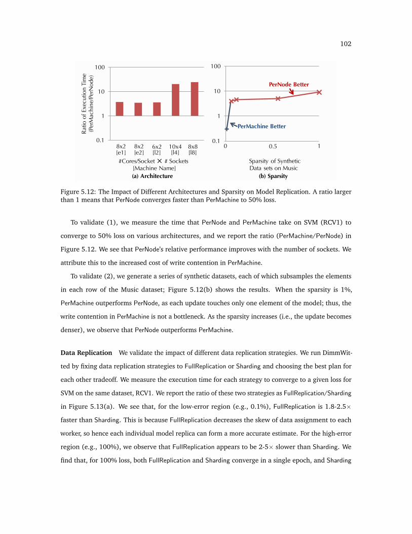
102
0.1
1
10
100
0.1
1
10
100
(a) Architecture
#Cores/Socket # Sockets [Machine Name]
Rat
io o
f Exe
cutio
n Ti
me
(Per
Mac
hine
/Per
Nod
e)
(b) Sparsity
Sparsity of SyntheticData sets on Music
PerMachine Better
PerNode Better
[e1] [e2] [l2] [l4] [l8]8x2 8x2 6x2 10x4 8x8 0 0.5 1
Figure 5.12: The Impact of Different Architectures and Sparsity on Model Replication. A ratio largerthan 1 means that PerNode converges faster than PerMachine to 50% loss.
To validate (1), we measure the time that PerNode and PerMachine take on SVM (RCV1) to
converge to 50% loss on various architectures, and we report the ratio (PerMachine/PerNode) in
Figure 5.12. We see that PerNode’s relative performance improves with the number of sockets. We
attribute this to the increased cost of write contention in PerMachine.
To validate (2), we generate a series of synthetic datasets, each of which subsamples the elements
in each row of the Music dataset; Figure 5.12(b) shows the results. When the sparsity is 1%,
PerMachine outperforms PerNode, as each update touches only one element of the model; thus, the
write contention in PerMachine is not a bottleneck. As the sparsity increases (i.e., the update becomes
denser), we observe that PerNode outperforms PerMachine.
Data Replication We validate the impact of different data replication strategies. We run DimmWit-
ted by fixing data replication strategies to FullReplication or Sharding and choosing the best plan for
each other tradeoff. We measure the execution time for each strategy to converge to a given loss for
SVM on the same dataset, RCV1. We report the ratio of these two strategies as FullReplication/Sharding
in Figure 5.13(a). We see that, for the low-error region (e.g., 0.1%), FullReplication is 1.8-2.5×
faster than Sharding. This is because FullReplication decreases the skew of data assignment to each
worker, so hence each individual model replica can form a more accurate estimate. For the high-error
region (e.g., 100%), we observe that FullReplication appears to be 2-5× slower than Sharding. We
find that, for 100% loss, both FullReplication and Sharding converge in a single epoch, and Sharding

103
(b)
1
10
100
Gibbs NN
Classic ChoiceDimmWitted
0
1
2
3
4
5
0.1% 1.0% 10.0% 100.0%
(a)
FullRepl. Better
Sharding Better
# V
aria
bles
/sec
ond
(Mill
ion)
Rat
io o
f Exe
c. T
ime
(Ful
lRep
l./Sh
ardi
ng)
Error to Optimal Loss Applications
Figure 5.13: (a) Tradeoffs of Data Replication. A ratio smaller than 1 means that FullReplication isfaster. (b) Performance of Gibbs Sampling and Neural Networks Implemented in DimmWitted.
may therefore be preferred, as it examines less data to complete that single epoch. In all of our
experiments, FullReplication is never substantially worse and can be dramatically better. Thus, if there
is available memory, the FullReplication data replication seems to be preferable.
5.2.4 Gibbs Sampling
We briefly describe how to run Gibbs sampling (which uses a column-to-row access method). Using
the same tradeoffs, we achieve a significant increase in speed over the classical implementation
choices of these algorithms.
Gibbs sampling is one of the most popular algorithms to solve statistical inference and learning
over probabilistic graphical models [159]. We briefly observe that its main step is a column-to-row
access. A factor graph can be thought of as a bipartite graph of a set of variables and a set of
factors. To run Gibbs sampling, the main operation is to select a single variable, and calculate the
conditional probability of this variable, which requires the fetching of all factors that contain this
variable and all assignments of variables connected to these factors. This operation corresponds to
the column-to-row access method. Similar to first-order methods, recently, a Hogwild! algorithm for
Gibbs was established [103]. As shown in Figure 5.13(b), applying the technique in DimmWitted to
Gibbs sampling achieves 4× the throughput of samples as the PerMachine strategy.

104
5.2.5 Conclusion to In-memory Statsitical Analytics
For statistical analytics on main-memory, NUMA-aware machines, we studied tradeoffs in access
methods, model replication, and data replication. We found that using novel points in this tradeoff
space can have a substantial benefit: our DimmWitted prototype engine can run at least one popular
task at least 100× faster than other competitor systems. This comparison demonstrates that this
tradeoff space may be interesting for current and next-generation statistical analytics systems.
5.3 Conclusion
In this chapter, we focus on speeding up the execution of statistical inference over a range of models,
e.g., logistic regression, support vector machines, and factor graphs. Our study considers two cases:
(1) the data fit in main memory and (2) the data does not fit in main memory. For both cases, we
study the system tradeoff of conducting statistical inference and learning, and our experiments show
that our study of the tradeoff contributes to up to two orders of magnitude speed up compared with
existing tools. The techniques we designed in this chapter helps the user of DeepDive to focus more
on integrating high-level knowledge, instead of low-level efficiency and scalability details.

105
6. Incremental Execution
We need to face up to the need for iterative procedures in data analysis. It is nice to plan to make
but a single analysis... it is also nice to be able to carry out an individual analysis in a single
straightforward step to avoid iteration and repeated computation. But it is not realistic to believe
that good data analysis is consistent with either of these niceties.
— John W. Tukey, The Future of Data Analysis, 1962
In previous chapters, we described how to write a DeepDive program to specify a KBC system and
how to execute it in an efficient and scalable way given a batch of documents. However, as we
described in Chapter 3, developing this KBC program is not an one-shot process; instead, it requires
the user to follow an iterative protocol to deciding on the right features, external sources, domain
knowledge, and supervision rules to use in a KBC program. This iterative protocol requires the user
to execute a series of KBC systems that differ only slightly from the others. In this chapter, we focus
on a different question that the previous chapter; instead of focusing on how to efficiently execute a
KBC system over a batch of documents and a given KBC program, we focus on the following question:
Can we make the execution of a series of KBC systems with slightly different KBC programs efficient?
We study this question in two ways. First, we focus on a problem called feature selection, in which
the user already knows a set of candidate features but wants to select a subset from these features.
By allowing the user to select a subset of features, we help her to better explain the KBC systems she
built and also help avoid overfitting. One observation is that the process of feature selection is often a
human-in-the-loop iterative process using automatic feature selection algorithms. The first technique
that we developed is a DSL language that enables iterative feature selection for a range of popular
statistical models, and we study how to make this process efficient. Our second focus is on how to
develop a set of new features, supervision rules, or domain knowledge rules instead of just selecting a
subset, which we call feature engineering. The second technique that we developed is a technique to
incrementally maintain the inference and learning results over factor graphs and validate it over five
KBC systems we built. As we will see, both techniques achieve up to two orders of magnitude speed
up on their target workloads. We describe these two techniques in this chapter.

106
6.1 Incremental Feature Selection
One of the most critical stages in the data analytics process is feature selection; in feature selection, an
analyst selects the inputs or features of a model to help improve modeling accuracy or to help an
analyst understand and explore their data. These features could come from a KBC system, e.g., to
select the subset of dependency paths between mention pairs that are actual indicators of relations;
or could come from other analytics tasks, e.g., bioinformatics, genomics, or business intelligence.
With the increased interest in data analytics, a pressing challenge is to improve the efficiency of
the feature selection process. In this work, we propose Columbus, the first data-processing system
designed to support the feature-selection process.
To understand the practice of feature selection, we interviewed analysts in enterprise settings.
This included an insurance company, a consulting firm, a major database vendor’s analytics customer,
and a major e-commerce firm. Uniformly, analysts agreed that they spend the bulk of their time on
the feature selection process. Confirming the literature on feature selection [89, 104], we found
that features are selected (or not) for many reasons: their statistical performance, their real-world
explanatory power, legal reasons,1 or for some combination. Thus, feature selection is practiced as
an interactive process with an analyst in the loop. Analysts use feature selection algorithms, data
statistics, and data manipulations as a dialogue that is often specific to their application domain.
Nevertheless, the feature selection process has structure: analysts often use domain-specific cookbooks
that outline best practices for feature selection [89].
Although feature selection cookbooks are widely used, the analyst must still write low-level code,
increasingly in R, to perform the subtasks in the cookbook that comprise a feature selection task.
In particular, we have observed that such users are forced to write their own custom R libraries to
implement simple routine operations in the feature selection literature (e.g., stepwise addition or
deletion [89]). Over the last few years, database vendors have taken notice of this trend, and now,
virtually every major database engine ships a product with some R extension: Oracle’s OR, IBM’s
SystemML [80], SAP HANA, and Revolution Analytics on Hadoop and Teradata. These R-extension
layers (RELs) transparently scale operations, such as matrix-vector multiplication or the determinant,
to larger sets of data across a variety of backends, including multicore main memory, database
engines, and Hadoop. We call these REL operations ROPs.
1Using credit score as a feature is considered a discriminatory practice by the insurance commissions in both Californiaand Massachusetts.
107
However, we observed that one major source of inefficiency in analysts’ code is not addressed by
ROP optimization: missed opportunities for reuse and materialization across ROPs. Our first contri-
bution is to demonstrate a handful of materialization optimizations that can improve performance
by orders of magnitude. Selecting the optimal materialization strategy is difficult for an analyst, as
the optimal strategy depends on the reuse opportunities of the feature selection task, the error the
analyst is willing to tolerate, and properties of the data and compute node, such as parallelism and
data size. Thus, an optimal materialization strategy for an R script for one dataset may not be the
optimal strategy for the same task on another data set. As a result, it is difficult for analysts to pick
the correct combination of materialization optimizations.
To study these tradeoffs, we introduce Columbus, an R language extension and execution frame-
work designed for feature selection. To use Columbus, a user writes a standard R program. Columbus
provides a library of several common feature selection operations, such as stepwise addition, i.e., “add
each feature to the current feature set and solve.” This library mirrors the most common operations
in the feature selection literature [89] and what we observed in analysts’ programs. Columbus’s
optimizer uses these higher-level, declarative constructs to recognize opportunities for data and
computation reuse. To describe the optimization techniques that Columbus employs, we introduce
the notion of a basic block.
A basic block is Columbus’s main unit of optimization. A basic block captures a feature selection
task for generalized linear models, which captures models like linear and logistic regression, support
vector machines, lasso, and many more; see Def. 6.1. Roughly, a basic block B consists of a data
matrix A ∈ RN×d , where N is the number of examples and d is the number of features, a target
b ∈ RN , several feature sets (subsets of the columns of A), and a (convex) loss function. A basic
block defines a set of regression problems on the same data set (with one regression problem for
each feature set). Columbus compiles programs into a sequence of basic blocks, which are optimized
and then transformed into ROPs. Our focus is not on improving the performance of ROPs, but on
how to use widely available ROPs to improve the performance of feature selection workloads.
We describe the opportunities for reuse and materialization that Columbus considers in a basic
block. As a baseline, we implement classical batching and materialization optimizations. In addition,
we identify three novel classes of optimizations, study the tradeoffs each presents, and then describe
a cost model that allows Columbus to choose between them. These optimizations are novel in that

108
Materialization Strategy Error Tolerance Sophistication of Tasks ReuseLazy
Low (Exact Solution)Medium
LowEager
Naıve Sampling High (Without Guarantee)HighCoreset Medium-High (With Guarantee) Small
QR Low (Exact Solution) Large
Table 6.1: A summary of tradeoffs in Columbus.
they have not been considered in traditional SQL-style analytics (but all the optimizations have been
implemented in other areas).
Subsampling Analysts employ subsampling to reduce the amount of data the system needs to
process to improve runtime or reduce overfitting. These techniques are a natural choice for analytics,
as both the underlying data collection process and solution procedures are only reliable up to some
tolerance. Popular sampling techniques include naıve random sampling and importance sampling
(coresets). Coresets [38,114] is a relatively recent importance-sampling technique; when d N ,
coresets allow one to create a sample whose size depends on d (the number of features)–as opposed
to N (the number of examples)–and that can achieve strong approximation results: essentially,
the loss is preserved on the sample for any model. In enterprise workloads (as opposed to web
workloads), we found that the overdetermined problems (d N), well-studied in classical statistics,
are common. Thus, we can use a coreset to optimize the result with provably small error. However,
computing a coreset requires computing importance scores that are more expensive than a naıve
random sample. We study the cost-benefit tradeoff for sampling-based materialization strategies. Of
course, sampling strategies have the ability to improve performance by an order of magnitude. On
a real data set, called Census,2 we found that d was 1000x smaller than N, as well as that using a
coreset outperforms a baseline approach by 89x, while still getting a solution that is within 1% of the
loss of the solution on the entire dataset.
Transformation Materialization Linear algebra has a variety of decompositions that are analogous
to sophisticated materialized views. One such decomposition, called a (thin) QR decomposition [81],
is widely used to optimize regression problems. Essentially, after some preprocessing, a QR decompo-
sition allows one to solve a class of regression problems in a single scan over the matrix. In feature
selection, one has to solve many closely related regression problems, e.g., for various subsets of
2https://archive.ics.uci.edu/ml/datasets/Census+Income

109
features (columns of A). We show how to adapt QR to this scenario as well. When applicable, QR
can outperform a baseline by more than 10×; QR can also be applied together with coresets, which
can result in 5× more speed up. Of course, there is a cost-benefit tradeoff that one must make when
materializing QR, and Columbus develops a simple cost model for this choice.
Model Caching Feature selection workloads require that analysts solve many similar problems.
Intuitively, it should be possible to reuse these partial results to “warmstart” a model and improve its
convergence behavior. We propose to cache several models, and we develop a technique that chooses
which model to use for a warmstart. The challenge is to be able to find “nearby” models, and we
introduce a simple heuristic for model caching. Compared with the default approach in R (initializing
with a random start point or all 0’s), our heuristic provides a 13x speedup; compared with a simple
strategy that selects a random model in the cache, our heuristic achieves a 6x speedup. Thus, the
cache and the heuristic contribute to our improved runtime.
We tease apart the optimization space along three related axes: error tolerance, the sophistication
of the task, and the amount of reuse (see Section 6.1.2). Table 6.1 summarizes the relationship
between these axes and the tradeoffs. Of course, the correct choice also depends on computational
constraints, notably parallelism. We describe a series of experiments to validate this tradeoff space
and find that no one strategy dominates another. Thus, we develop a cost-based optimizer that
attempts to select an optimal combination of the above materialization strategies. We validate that
our heuristic optimizer has performance within 10% of the optimal optimization strategy (found
offline by brute force) on all our workloads. Many of the subproblems of the optimizer are classically
NP-hard, justifying heuristic optimizers.
Contributions This section makes three contributions: (1) We propose Columbus, which is the
first data processing system designed to support the feature selection dialogue; (2) we are the first
to identify and study both existing and novel optimizations for feature selection workloads as data
management problems; and (3) we use the insights from (2) to develop a novel cost-based optimizer.
We validate our results on several real-world programs and datasets patterned after our conversations
with analysts. Additionally, we validate Columbus across two backends from main memory and REL
for an RDBMS. We argue that these results suggest that feature selection is a promising area for

110
1 e = SetErrorTolerance(0.01) # Set Error Tolerance2 d1 = Dataset(“USCensus”) # Register the dataset3 s1 = FeatureSet(“NumHouses”, ...) # Population-related features4 l1 = CorrelationX(s1, d1) # Get mutual correlations5 s1 = Remove(s1, “NumHouses”) # Drop the feature “NumHouses”6 l2 = CV(lsquares_loss, s1, d1, k=5) # Cross validation (least squares)7 d2 = Select(d1,“Income >= 10000”) # Focus on high-income areas8 s2 = FeatureSet(“Income”, ...) # Economic features9 l3 = CV(logit_loss, s2, d2, k=5) # Cross validation with (logit loss)
10 s3 = Union(s1, s2) # Use both sets of features11 s4 = StepAdd(logit_loss, s3, d1) # Add in one other feature12 Final(s4) # Session ends with chosen features
Figure 6.1: Example snippet of a Columbus program.
future data management research. Additionally, we are optimistic that the technical optimizations we
pursue apply beyond feature selection to areas like scientific databases and tuning machine learning.
Outline The rest of this section is organized as follows. In Section 6.1.1, we provide an overview
of the Columbus system. In Section 6.1.2, we describe the tradeoff space for executing a feature
selection program and our cost-based optimizer. We describe experimental results in Section 6.1.3.
We discuss related work in Chapter 7.
The key task of Columbus is to compile and optimize an extension of the R language for feature
selection. We compile this language into a set of REL operations, which are R-language constructs
implemented by today’s language extenders, including ORE, Revolution Analytics, etc. One key
design decision in Columbus is not to optimize the execution of these REL operators; these have
already been studied intensively and are the subjects of major ongoing engineering efforts. Instead,
we focus on how to compile our language into the most common of these REL operations (ROPs).
Figure 6.3 shows all ROPs that are used in Columbus.
6.1.1 System Overview
6.1.1.1 Columbus Programs
In Columbus, a user expresses their feature selection program against a set of high-level constructs
that form a domain specific language for feature selection. We describe these constructs next, and
we selected these constructs by talking to a diverse set of analysts and following the state-of-the-art

111
Logical OperatorsData Transform Select, Join, Union, ...
EvaluateMean, Variance, Covariance, Pearson Correlation
Cross Validation, AICRegression Least Squares, Lasso, Logistic Regression
ExploreFeature Set Operation
Stepwise Addition, Stepwise DeletionForward Selection, Backward Selection
Table 6.2: A summary of operators in Columbus.
ROPs
A=DataSet(“A”)fs1=FeatureSet(f1, f2)fs2=FeatureSet(f3)fs3=StepDrop(A, fs1)fs4=UNION(fs3, fs2)
fs1=f1,f2fs2=f3fs3=f1fs4=f1, f3
Parser
Basic BlocksColumbus Program Execution Result
Optimizer Executor
A, loss=LR, εF1=f1, F2=f2
UNION
fs4
Basic BlockStandard ROP
qr(A[,fs1])
backsolve(…)
backsolve(…)
UNION
fs2
Figure 6.2: Architecture of Columbus.
literature in feature selection. Columbus’s language is a strict superset of R, so the user still has access
to the full power of R.3 We found that this flexibility was a requirement for most of the analysts
surveyed. Figure 6.1 shows an example snippet of a Columbus program. For example, the 9th line of
the program executes logistic regression and reports its score using cross validation.
Columbus has three major datatypes: A data set, which is a relational table R(A1, . . . , Ad).4 A
feature set F for a dataset R(A1, . . . , Ad) is a subset of the attributes F ⊆ A1, . . . , Ad. A model
for a feature set is a vector that assigns each feature a real-valued weight. As shown in Table 6.2,
Columbus supports several operations. We classify these operators based on what types of output
an operator produces and order the classes in roughly increasing order of the sophistication of
optimization that Columbus is able to perform for such operations (see Table 6.2 for examples):
(1) Data Transformation Operations, which produce new data sets; (2) Evaluate Operations, which
evaluate data sets and models; (3) Regression Operations, which produce a model given a feature set;
and (4) Explore Operations, which produce new feature sets:
(1) Data Transform. These operations are standard data manipulations to slice and dice the
3We also have expressed the same language over Python, but for simplicity, we stick to the R model in this section.4Note that the table itself can be a view; this is allowed in Columbus, and the tradeoffs for materialization are standard,
so we omit the discussion of them in the section.

112
dataset. In Columbus, we are aware only of the schema and cardinality of these operations; these
operations are executed and optimized directly using a standard RDBMS or main-memory engine. In
R, the frames can be interpreted either as a table or an array in the obvious way. We map between
these two representations freely.
(2) Evaluate. These operations obtain various numeric scores given a feature set including
descriptive scores for the input feature set, e.g., mean, variance, or Pearson correlations and scores
computed after regression, e.g., cross-validation error (e.g., of logistic regression), and Akaike
Information Criterion (AIC) [89]. Columbus can optimize these calculations by batching several
together.
(3) Regression. These operations obtain a model given a feature set and data, e.g., models
trained by using logistic regression or linear regression. The result of a regression operation is often
used by downstream explore operations, which produces a new feature set based on how the previous
feature set performs. These operations also take a termination criterion (as they do in R): either the
number of iterations or until an error criterion is met. Columbus supports either of these conditions
and can perform optimizations based on the type of model (as we discuss).
(4) Explore. These operations enable an analyst to traverse the space of feature sets. Typically,
these operations result in training many models. For example, a STEPDROP operator takes as input a
data set and a feature set, and outputs a new feature set that removes one feature from the input by
training a model on each candidate feature set. Our most sophisticated optimizations leverage the
fact that these operations operate on features in bulk. The other major operation is STEPADD. Both
are used in many workloads and are described in Guyon et al. [89].
Columbus is not intended to be comprehensive. However, it does capture the workloads of several
analysts that we observed, so we argue that it serves as a reasonable starting point to study feature
selection workloads.
6.1.1.2 Basic Blocks
In Columbus, we compile a user’s program into a directed-acyclic-dataflow graph with nodes of two
types: R functions and an intermediate representation called a basic block. The R functions are opaque
to Columbus, and the central unit of optimization is the basic block (extensible optimizers [85]).
Definition 6.1. A task is a tuple t = (A, b, `, ε, F,R) where A ∈ RN×d is a data matrix, b ∈ RN is a

113
label (or target), ` : R2 → R+ is a loss function, ε > 0 is an error tolerance, F ⊆ [d] is a feature set, and
R ⊆ [N ] is a subset of rows. A task specifies a regression problem of the form:
Lt(x) =∑i∈R
`(zi, bi) s.t. z = AΠFx
Here ΠF is the axis-aligned projection that selects the columns or feature sets specified by F .5 Denote an
optimal solution of the task x∗(t) defined as
x∗(t) = argminx∈Rd
Lt(x)
Our goal is to find an x(t) that satisfies the error6
‖Lt(x(t))− Lt(x∗(t))‖2 ≤ ε
A basic block, B, is a set of tasks with common data (A, b) but with possibly different feature sets F and
subsets of rows R.
Columbus supports a family of popular non-linear models, including support vector machines,
(sparse and dense) logistic regression, `p regression, lasso, and elastic net regularization. We give an
example to help clarify the definition.
Example 6.2. Consider the 6th line in Figure 6.1, which specifies a five-fold cross validation operator
with least squares over data set d1 and feature set s1. Columbus will generate a basic block B with five
tasks, one for each fold. Let ti = (A, b, l, ε, F,R). Then, A and b are defined by the data set d1 and
l(x, b) = (x − b)2. The error tolerance ε is given by the user in the 1st line. The projection of features
F = s1 is found by a simple static analysis. Finally, R corresponds to the set of examples that will be
used by the ith fold.
The basic block is the unit of Columbus’s optimization. Our design choice is to combine several
operations on the same data at a high-enough level to facilitate bulk optimization, which is our focus
in the next section.
5For F ⊆ [d], ΠF ∈ Rd×d where (ΠF )ii = 1 if i ∈ F and all other entries are 0.6We allow termination criteria via a user-defined function or the number of iterations. The latter simplifies reuse
calculations in Section 6.1.2, while arbitrary code is difficult to analyze (we must resort to heuristics to estimate reuse). Wepresent the latter as the termination criterion to simplify the discussion and as it brings out interesting tradeoffs.

114
Columbus’s compilation process creates a task for each regression or classification operator in
the program; each of these specifies all of the required information. To enable arbitrary R code, we
allow black box code in this work flow, which is simply executed. Selecting how to both optimize and
construct basic blocks that will execute efficiently is the subject of Section 6.1.2.
REL Operations To execute a program, we compile it into a sequence of REL Operations (ROPs).
These are operators that are provided by the R runtime, e.g., R and ORE. Figure 6.3 summarizes the
host-level operators that Columbus uses, and we observe that these operators are present in both R
and ORE. Our focus is how to optimize the compilation of language operators into ROPs.
6.1.1.3 Executing a Columbus Program
To execute a Columbus program, our prototype contains three standard components, as shown in
Figure 6.2: (1) parser; (2) optimizer; and (3) executor. At a high-level, these three steps are similar
to the existing architecture of any data processing system. The output of the parser can be viewed as
a directed acyclic graph, in which the nodes are either basic blocks or standard ROPs, and the edges
indicate data flow dependency. The optimizer is responsible for generating a “physical plan.” This
plan defines which algorithms and materialization stategies are used for each basic block; the relevant
decisions are described in Sections 6.1.2.1 and 6.1.2.2. The optimizer may also merge basic blocks
together, which is called multiblock optimization, which is described in Section 6.1.2.4. Finally, there
is a standard executor that manages the interaction with the REL and issues concurrent requests.
6.1.2 The Columbus Optimizer
We begin with optimizations for a basic block that has a least-squares cost, which is the simplest
setting in which Columbus’s optimizations apply. We then describe how to extend these ideas to
basic blocks that contain nonlinear loss functions and then describe a simple technique called model
caching.
Optimization Axes To help understand the optimization space, we present experimental results on
the CENSUS data set using Columbus programs modeled after our experience with insurance analysts.

115
ROPs Semantic Cost
A <- B[1:n,1:d] matrix sub-selection DN+dn
A %*% C matrix multiplication dnm
A * E element-wise multiplication dn
solve(W [,b]) calculate W-1 or W-1b d3
qr(A) QR decomposition of A d2n
sample(V, prob) Sample element in V with prob n
backsolve(W [,b]) solve() for triangular matrix W d2
A: nd B: ND C: dmE: nd V: n1 W: dd
Materialization Strategies Materialization ROPs Execution ROPs
Lazy N/A <-, %*%, solve
Eager <- %*%, solve
Naïve Sampling <-, sample %*%, solve
Coreset <-, %*%, solve, sample, * %*%, solve
QR <-, qr backsolve
The cost of an op. with black font face dominates the cost of any green op. for that ROP.
(b) Materialization Strategies and ROPs Used by Each Strategy
(a) ROPs Used in Columbus and Their Running Times
Legend
Figure 6.3: (a) ROPs used in Columbus and their costs; (b) Cost model of materializations inColumbus. When data are stored in main memory, the cost for matrix sub-selection (a← B[1 : n, 1 :d]) is only dn. In (b), Materialization ROPs are the set of ROPs used in the materialization phasefor an operator, while Execution ROPs are those ROPs used during execution (i.e., while solving themodel). The materialization cost and execution cost for each strategy can be estimated by summingthe cost of each ROPs they produce in (a).
Figure 6.4 illustrates the crossover points for each optimization opportunity along three axes that we
will refer to throughout this section:7
(1) Error tolerance depends on the analyst and task. For intuition, we think of different types of
error tolerances, with two extremes: error tolerant ε = 0.5 and high quality ε = 10−3. In Figure 6.4,
we show ε ∈ 0.001, 0.01, 0.1, 0.5.
(2) Sophistication of the feature selection task, namely the loss function (linear or not), the
number of feature sets or rows selected, and their degree of overlap. In Figure 6.4, we set the number
of features as 10, 100, 161 and the number of tasks in each block as 1, 10, 20, 50.7For each combination of parameters below, we execute Columbus and record the total execution time in a main memory
R backend. This gives us about 40K data points, and we only summarize the best results in this section. Any omitted datapoint is dominated by a shown data point.

116
0
10
20
30
40
0 5 100
5
10
0.001 0.01 0.1 10
5
10
15
20
0 100 2000
10
20
30
0 0.5 10
10
20
30
40
0 10 20
Tota
l Tim
e (s
econ
ds)
(a) Error Tolerance (ε) (b) # Features (c) Size of Overlapping Feature Sets
(e) # Threads
LazyQR
Coreset+QR Coreset
Error Tolerance Sophistication of Task and Reuse Computation
Coreset+QR
Lazy
Coreset+QR
Coreset+QR
QR
Lazy
(d) # Iterations
Lazy
QR
Figure 6.4: An Illustration of the Tradeoff Space of Columbus, which is defined in Section 6.1.2.
(3) Reuse is the degree to which we can reuse computation (and that it is helpful to do so).
The key factors are the amount of overlap in the feature sets in the workloads8 and the number of
available threads that Columbus uses, which we set here to 1, 5, 10, 20.9
We discuss these graphs in paragraphs marked Tradeoff.
6.1.2.1 A Single, Linear Basic Block
We consider three families of optimizations: (1) classical database optimizations, (2) sampling-based
optimizations, and (3) transformation-based optimizations. The first optimization is essentially
unaware of the feature-selection process; in contrast, the last two of these leverage the fact that we
are solving several regression problems. Each of these optimizations can be viewed as a form of
precomputation (materialization). Thus, we describe the mechanics of each optimization, the cost it
incurs in materialization, and its cost at runtime. Figure 6.3 summarizes the cost of each ROP and
the dominant ROP in each optimization. Because each ROP is executed once, one can estimate the
cost of each materialization from this figure.10
To simplify our presentation, in this subsection, we let `(x, b) = (x− b)2, i.e., the least-squares
loss, and suppose that all tasks have a single error ε. We return to the more general case in the next
subsection. Our basic block can be simplified to B = (A, b, F , R, ε), for which we compute:
x(R,F ) = argminx∈Rd
‖ΠR (AΠFx− b) ‖22 where R ∈ R, F ∈ F
8Let G = (∪F∈FF,E) be a graph, in which each node corresponds to a feature. An edge (f1, f2) ∈ E if there existsF ∈ F such that f1, f2 ∈ F . We use the size of the largest connected component in G as a proxy for overlap.
9Note that Columbus supports two execution models, namely batch mode and interactive mode.10We ran experiments on three different types of machines to validate that the cost we estimated for each operator is close
to the actual running time.

117
Our goal is to compile the basic block into a set of ROPs. We explain the optimizations that we
identify below.
Classical Database Optimizations We consider classical eager and lazy view materialization
schemes. Denote F∪ = ∪F∈FF and R∪ = ∪R∈R in the basic block. It may happen that A contains
more columns than F∪ and more rows than R∪. In this case, one can project away these extra rows
and columns—analogous to materialized views of queries that contain selections and projections. As
a result, classical database materialized view optimizations apply. Specially, Columbus implements
two strategies, namely Lazy and Eager. The Lazy strategy will compute these projections at execution
time, and Eager will compute these projections at materialization time and use them directly at
execution time. When data are stored on disk, e.g., as in ORE, Eager could save I/Os versus Lazy.
Tradeoff Not surprisingly, Eager has a higher materialization cost than Lazy, while Lazy has a
slightly higher execution cost than Eager, as one must subselect the data. Note that if there is ample
parallelism (at least as many threads as feature sets), then Lazy dominates. The standard tradeoffs
apply, and Columbus selects between these two techniques in a cost-based way. If there are disjoint
feature sets F1 ∩ F2 = ∅, then it may be more efficient to materialize these two views separately. The
general problem of selecting an optimal way to split a basic block to minimize cost is essentially a
weighted set cover, which is NP-hard. As a result, we use a simple heuristic: split disjoint feature
sets. With a feature selection workload, we may know the number of times a particular view will be
reused, which Columbus can use to more intelligently chose between Lazy and Eager (rather than
not having this information). These methods are insensitive to error and the underlying loss function,
which will be major concerns for our remaining feature-selection-aware methods.
Sampling-Based Optimizations Subsampling is a popular method to cope with large data and long
runtimes. This optimization saves time simply because one is operating on a smaller dataset. This
optimization can be modeled by adding a subset selection (R ∈ R) to a basic block. In this section, we
describe two popular methods: naıve random sampling and a more sophisticated importance-sampling
method called coresets [38,114]; we describe the tradeoffs these methods provide.
Naıve Sampling Naıve random sampling is widely used, and in fact, analysts often ask for it
by name. In naıve random sampling, one selects some fraction of the data set. Recall that A has N

118
rows and d columns; in naıve sampling, one selects some fraction of the N rows (say 10%). The
cost model for both materialization and its savings of random sampling is straightforward, as one
performs the same solve—only on a smaller matrix. We perform this sampling using the ROP SAMPLE.
Coresets A recent technique called coresets allows one to sample from an overdetermined system
A ∈ RN×d with a sample size that is proportional to d and independent of N with much stronger
guarantees than naıve sampling. In some enterprise settings, d (the number of features) is often
small (say 40), but the number of data points is much higher, say millions, and coresets can be a
large savings. We give one such result:
Proposition 6.3 (Boutsidis et al. [38]). For A ∈ RN×d and b ∈ RN . Define s(i) = aTi(ATA
)−1ai.
Let A and b be the result of sampling m rows, where row i is selected with probability proportional to
s(i). Then, for all x ∈ Rd, we have
Pr
[∣∣∣∣‖Ax− b‖22 − N
m‖Ax− b‖22
∣∣∣∣ < ε‖Ax− b‖22]>
1
2
So long as m > 2ε−2d log d.
This guarantee is strong.11 To understand how strong, observe that naıve sampling cannot meet
this type of guarantee, without sampling proportional to N . To see this, consider the case in which a
feature occurs in only a single example, e.g., A1,1 = 1 and Ai,1 = 0 for i = 2, . . . , N . It is not hard to
see that the only way to achieve a similar guarantee is to make sure the first row is selected. Hence,
naıve sampling will need roughly N samples to guarantee this is selected. Note that Prop 6.3 does
not use the value b. Columbus uses this fact later to optimize basic blocks with changing b.
Tradeoff Looking at Figure 6.4, one can see a clear tradeoff space: coresets require two passes
over the data to compute the sensitivity scores. However, the smaller sample size (proportional to d)
can be a large savings when the error ε is moderately large. But as either d or ε−1 grows, coresets
become less effective, and there is a cross-over point. In fact, coresets are useless when N = d.
One benefit of coresets is that they have explicit error guarantees in terms of ε. Thus, our current
implementation of Columbus will not automatically apply Naıve Sampling unless the user requests it.
With optimal settings for sample size, naıve sampling can get better performance than coresets.
11Note that one can use log2 δ−1 independent trials to boost the probability of success to 1− δ.

119
Transformation-Based Optimizations In linear algebra, there are decomposition methods to solve
(repeated) least-squares efficiently; the most popular of these is called the QR decomposition [81]. At
a high level, we use the QR decomposition to transform the data matrix A so that many least-squares
problems can be solved efficiently. Typically, one uses a QR to solve for many different values of b
(e.g., in Kalman filter updates). However, in feature selection, we use a different property of the QR:
that it can be used across many different feature sets. We define the QR factorization (technically the
thin QR), describe how Columbus uses it, and then describe its cost model.
Definition 6.4 (Thin QR Factorization). The QR decomposition of a matrix A ∈ RN×d is a pair of
matrices (Q,R) where Q ∈ RN×d, R ∈ Rd×d, and A=QR. Q is an orthogonal matrix, i.e., QTQ = I
and R is upper triangular.
We observe that since Q−1 = QT and R is upper triangular, one can solve Ax = b by setting
QRx = b and multiplying through by the transpose of Q so that Rx = QT b. Since R is upper
triangular, one can solve can this equation with back substitution; back substitution does not require
computing the inverse of R, and its running time is linear in the number of entries of R, i.e., O(d2).
Columbus leverages a simple property of the QR factorization: upper triangular matrices are
closed under multiplication, i.e., if U is upper triangular, then so is RU . Since ΠF is upper triangular,
we can compute many QR factorizations by simply reading off the inverse of RΠF .12 This simple
observation is critical for feature selection. Thus, if there are several different row selectors, Columbus
creates a separate QR factorization for each.
Tradeoff As summarized in Figure 6.3, QR’s materialization cost is similar to importance
sampling. In terms of execution time, Figure 6.4 shows that QR can be much faster than coresets:
solving the linear system is quadratic in the number of features for QR but cubic for coresets (without
QR). When there are a large number of feature sets and they overlap, QR can be a substantial win
(this is precisely the case when coresets are ineffective). These techniques can also be combined,
which further modifies the optimal tradeoff point. An additional point is that QR does not introduce
error (and is often used to improve numerical stability), which means that QR is applicable in error
tolerance regimes when sampling methods cannot be used.
12Notice that ΠRQ is not necessarily orthogonal, so ΠRQ may be expensive to invert.

120
Discussion of Tradeoff Space Figure 6.4 shows the crossover points for the tradeoffs we described
in this section for the CENSUS dataset. We describe why we assert that each of the following aspects
affects the tradeoff space.
Error For error-tolerant computation, naıve random sampling provides dramatic performance
improvements. However, when low error is required, then one must use classical database optimiza-
tions or the QR optimization. In between, there are many combinations of QR, coresets, and sampling
that can be optimal. As we can see in Figure 6.4(a), when the error tolerance is small, coresets are
significantly slower than QR. When the tolerance is 0.01, the coreset we need is even larger than the
original data set, and if we force Columbus to run on this large coreset, it would be more than 12x
slower than QR. For tolerance 0.1, coreset is 1.82x slower than QR. We look into the breakdown of
materialization time and execution time, and we find that materialization time contributes to more
than 1.8x of this difference. When error tolerance is 0.5, Coreset+QR is 1.37x faster than QR. We
ignore the curve for Lazy and Eager because they are insensitive to noises and are more than 1.24x
slower than QR.
Sophistication One measure of sophistication is the number of features the analyst is consider-
ing. When the number of features in a basic block is much smaller than the data set size, coresets
create much smaller but essentially equivalent data sets. As the number of features, d, increases,
or the error decreases, coresets become less effective. On the other hand, optimizations, like QR,
become more effective in this regime: although materialization for QR is quadratic in d, it reduces
the cost to compute an inverse from roughly d3 to d2.
As shown in Figure6.4(b), as the number of features grows, CoreSet+QR slows down. With 161
features, the coreset will be larger than the original data set. However, when the number of features
is small, the gap between CoreSet+QR and QR will be smaller. When the number of features is 10,
CoreSet+QR is 1.7x faster than QR. When the number of feature is small, the time it takes to run a
QR decomposition over the coreset could be smaller than over the original data set, hence, the 1.7x
speedup of CoreSet+QR over QR.
Reuse In linear models, the amount of overlap in the feature sets correlates with the amount of
reuse. We randomly select features but vary the size of overlapping feature sets. Figure6.4(c) shows
the result. When the size of the overlapping feature sets is small, Lazy is 15x faster than CoreSet+QR.

121
This is because CoreSet wastes time in materializing for a large feature set. Instead, Lazy will solve
these problems independently. On the other hand, when the overlap is large, CoreSet+QR is 2.5x
faster than Lazy. Here, CoreSet+QR is able to amortize the materialization cost by reusing it on
different models.
Available Parallelism If there is a large amount of parallelism and one needs to scan the data
only once, then a lazy materialization strategy is optimal. However, in feature selection workloads
where one is considering hundreds of models or repeatedly iterating over data, parallelism may be
limited, so mechanisms that reuse the computation may be optimal. As shown by Figure 6.4(e), when
the number of threads is large, Lazy is 1.9x faster than CoreSet+QR. The reason is that although the
reuse between models is high, all of these models could be run in parallel in Lazy. Thus, although
CoreSet+QR does save computation, it does not improve the wall-clock time. On the other hand,
when the number of threads is small, CoreSet+QR is 11x faster than Lazy.
6.1.2.2 A Single, Non-linear Basic Block
We extend our methods to non-linear loss functions. The same tradeoffs from the previous section
apply, but there are two additional techniques we can use. We describe them below.
Recall that a task solves the problem
minx∈Rd
N∑i=1
`(zi, bi) subject to z = Ax
where ` : R2 → R+ is a convex function.
Iterative Methods We select two methods: stochastic gradient descent (SGD) [31,37,169], and
iterative reweighted least squares (IRLS), which is implemented in R’s generalized linear model
package.13 We describe an optimization, warmstarting, that applies to such models as well as to
ADMM.
ADMM There is a classical, general purpose method that allows one to decompose such a problem
into a least-squares problem and a second simple problem. The method we explore is one of the most
popular, called the Alternating Direction Method of Multipliers (ADMM) [39], which has been widely
13stat.ethz.ch/R-manual/R-patched/library/stats/html/glm.html

122
used since the 1970s. We explain the details of this method to highlight a key property that allows us
to reuse the optimizations from the previous section.
ADMM is iterative and defines a sequence of triples (xk, zk, uk) for k = 0, 1, 2, . . . . It starts
by randomly initializing the three variables (x0, z0, u0), which are then updated by the following
equations:
x(k+1) = argminx
ρ
2||Ax− z(k) + u(k)||22
z(k+1) = argminz
N∑i=1
l(zi, bi) +ρ
2||Ax(k+1) − z + u(k)||22
u(k+1) = u(k) +Ax(k+1) − z(k+1)
The constant ρ ∈ (0, 2) is a step size parameter that we set by a grid search over five values.
There are two key properties of the ADMM equations that are critical for feature selection
applications:
(1) Repeated Least Squares The solve for x(k+1) is a linear basic block from the previous section
since z and u are fixed and the A matrix is unchanged across iteration. In nonlinear basic blocks,
we solve multiple feature sets concurrently, so we can reuse the transformation optimizations of the
previous section for each such update. To take advantage of this, Columbus logically rewrites ADMM
into a sequence of linear basic blocks with custom R functions.
(2) One-dimensional z We can rewrite the update for z into a series of independent, one-
dimensional problems. That is,
z(k+1)i = argmin
zi
l(zi, bi) +ρ
2(qi − zi)2, where q = Ax(k+1) + u(k)
This one-dimensional minimization can be solved by fast methods, such as bisection or Newton. To
update x(k+1), the bottleneck is the ROP “solve,” whose cost is in Figure 6.3. The cost of updating z
and u is linear in the number of rows in A, and can be decomposed into N problems that may be
solved independently.

123
Tradeoffs In Columbus, ADMM is our default solver for non-linear basic blocks. Empirically, on
all of our applications in our experiments, if one first materializes the QR computation for the least-
squares subproblem, then we find that ADMM converges faster than SGD to the same loss. Moreover,
there is sharing across feature sets that can be leveraged by Columbus in ADMM (using our earlier
optimization about QR). One more advanced case for reuse is when we must fit hyperparameters,
like ρ above or regularization parameters; in this case, ADMM enables opportunities for high degrees
of sharing.
6.1.2.3 Warmstarting by Model-Caching
In feature selection workloads, our goal is to solve a model after having solved many similar models.
For iterative methods like gradient descent or ADMM, we should be able to partially reuse these
similar models. We identify three situations in which such reuse occurs in feature-selection workloads:
(1) We downsample the data, learn a model on the sample, and then train a model on the original
data. (2) We perform stepwise removal of a feature in feature selection, and the “parent” model with
all features is already trained. (3) We examine several nearby feature sets interactively. In each case,
we should be able to reuse the previous models, but it would be difficult for an analyst to implement
effectively in all but the simplest cases. In contrast, Columbus can use warmstart to achieve up to
13x performance improvement for iterative methods without user intervention.
Given a cache of models, we need to choose a model: we observe that computing the loss of each
model on the cache on a sample of the data is inexpensive. Thus, we select the model with the lowest
sampled loss. To choose models to evict, we simply use an LRU strategy. In our workloads, the cache
does not become full, so we do not discuss it. However, if one imagines several analysts running
workloads on similar data, the cache could become a source of challenges and optimizations.
6.1.2.4 Multiblock Optimization
There are two tasks we need to do across blocks: (1) We need to decide on how coarse or fine to
make a basic block, and (2) we need to execute the sequence of basic blocks across the backend.
Multiblock Logical Optimization Given a sequence of basic blocks from the parser, Columbus
must first decide how coarse or fine to create individual blocks. Cross validation is, for example,
merged into a single basic block. In Columbus, we greedily improve the cost using the obvious

124
Features Tuples Size# Basic # Tasks # Lines Type ofBlocks /Basic Blocks of Code Basic Blocks
KDD 481 191 K 235 MB 6 10 28 6 LR BlocksCensus 161 109 K 100 MB 4 0.2 K 16 3 LS, 1 LRMusic 91 515 K 1 GB 4 0.1 K 16 3 LS, 1 LRFund 16 74 M 7 GB 1 2.5 K 4 1 LSHouse 10 2 M 133 MB 1 1.0 K 4 1 LS
Table 6.3: Dataset and Program Statistics. LS refers to Least Sqaures. LR refers to Logistic Regression.
estimates from Figure 6.3. The problem of deciding the optimal partitioning of many feature sets
is NP-hard by a reduction to WEIGHTEDSETCOVER. The intuition is clear, as one must cover all the
different features with as few basic blocks as possible. However, the heuristic merging can have large
wins, as operations like cross validation and grid searching parameters allow one to find opportunities
for reuse.
Cost-based Execution Recall that the executor of Columbus executes ROPs by calling the required
database or main-memory backend. The executor is responsible for executing and coordinating
multiple ROPs that can be executed in parallel; Columbus executor simply creates one thread to
manage each of these ROPs. The actual execution of each physical operator is performed by the
backend statistical framework, e.g., R or ORE. Nevertheless, we need to decide how to schedule these
ROPs for a given program. We experimented with the tradeoff of how coarsely or finely to batch the
execution. Many of the straightforward formulations of the scheduling problems are, not surprisingly,
NP-hard. Nevertheless, we found that a simple greedy strategy (to batch as many operators as
possible, i.e., operators that do not share data flow dependencies) was within 10% of the optimal
schedule obtained by a brute-force search. After digging into this detail, we found that many of the
host-level substrates already provide sophisticated data processing optimizations (e.g. sharing scans).
6.1.3 Experiments
Using the materialization tradeoffs we have outlined, we validate that Columbus is able to speed up
the execution of feature selection programs by orders of magnitude compared to straightforward
implementations in state-of-the-art statistical analytics frameworks across two different backends: R
(in-memory) and a commercial RDBMS. We validate the details of our technical claims about the
tradeoff space of materialization and our (preliminary) multiblock optimizer.

125
1
10
100
1000
10000
KDD Census Music Fund House1
10
100
1000
10000
100000
KDD Census Music Fund House
Exec
utio
n Ti
me
(sec
onds
) VanilladbOPT
Columbus Slowdown
Lazy 4.3x
Eager 1.1x
CoreSet 1.9x
QR 37.2x
(a) R Backend (b) DB-R Backend (c) Lesion Study on Census1.49x
183x
Figure 6.5: End-to-end Performance of Columbus. All approaches return a loss within 1% optimalloss.
6.1.3.1 Experiment Setting
Based on conversations with analysts, we selected a handful of datasets and created programs that
use these datasets to mimic analysts’ tasks in different domains. We describe these programs and
other experimental details.
Datasets and Programs To compare the efficiency of Columbus with baseline systems, we select
five publicly available data sets: (1) Census, (2) House, (3) KDD, (4) Music, and (5) Fund.14 These
data sets have different sizes, and we show the statistics in Table 6.3. We categorize them by the
number of features in each data set.
Both House, a dataset for predicting household electronic usage, and Fund, a dataset for predict-
ing the donation that a given agency will receive each year, have a small number of features (fewer
than 20). In these data sets, it is feasible to simply try and score almost all combinations of features.
We mimic this scenario by having a large basic block that regresses a least-squares model on feature
sets of sizes larger than 5 on House and 13 on Fund and then scores the results using AIC. These
models reflect a common scenario in current enterprise analytics systems.
At the other extreme, KDD has a large number of features (481), and it is infeasible to try many
combinations. In this scenario, the analyst is guided by automatic algorithms, like Lasso [184] (that
selects a few sparse features), manual intervention (moving around the feature space), and heavy use
of cross-validation techniques.15 Census is a dataset for the task of predicting mail responsiveness of
people in different Census blocks, each of which contains a moderate number of features (161). In
14These data sets are publicly available on Kaggle (www.kaggle.com/) or the UCI Machine Learning Repository. (archive.ics.uci.edu/ml/)
15 The KDD program contains six basic blocks, each of which is a 10-fold cross-validation. These six different basic blockswork on non-overlappings set of features specified by the user manually.

126
this example, analysts use a mix of automatic and manual specification tasks that are interleaved.16
This is the reason that we select this task for our running example. Music is similar to Census, and
both programs contain linear models (least squares) and non-linear models (logistic regression) to
mimic the scenario in which an analyst jointly explores the feature set to select and the model to use.
R Backends We implemented Columbus on multiple backends and report on two: (1) R, which is
the standard, main-memory R and (2) DB-R, commercial R implementation over RDBMS. We use R
2.15.2, and the most recent available versions of the commercial systems.
For all operators, we use the result of the corresponding main memory R function as the gold
standard. All experiments are run on instances on Amazon EC2 (cr1.8xlarge), which has 32 vCPU,
244 GB RAM, and 2x120GB SSD and runs Ubuntu 12.04.17
6.1.3.2 End-to-End Efficiency
We validate that Columbus improves the end-to-end performance of feature selection programs.
We construct two families of competitor systems (one for each backend): VANILLA, and DBOPT.
VANILLA is a baseline system that is a straightforward implementation of the corresponding feature
selection problem using the ROPs; thus it has the standard optimizations. DBOPT is Columbus, but
we enable only the optimizations that have appeared in classical database literature, i.e., Lazy, Eager,
and batching. DBOPT and Columbus perform scheduling in the same way to improve parallelism to
isolate the contributions of the materialization. Figure 6.5 shows the result of running these systems
over all five data sets with error tolerance ε set to 0.01.
On the R-based backend, Columbus executes the same program using less time than R on all
datasets. On Census, Columbus is two orders of magnitude faster, and on Music and Fund, Columbus
is one order of magnitude faster. On Fund and House, Columbus chooses to use CoreSet+QR as the
materialization strategy for all basic blocks and chooses to use QR for other data sets. This is because
for data sets that contain fewer rows and more columns, QR dominates CoreSet-based approaches,
as described in the previous Section. One reason that Columbus improves more on Census than on
Music and Fund is that Census has more features than Music and Fund; therefore, operations like
StepDrop produce more opportunities for reuse than Census.
16 The Census program contains four basic blocks, each of which is a STEPDROP operation on the feature set output by theprevious basic block.
17We also run experiments on other dedicated machines. The tradeoff space is similar to what we report in this section.

127
To understand the classical points in the tradeoff space, compare the efficiency of DBOPT with
the baseline system, VANILLA. When we use R as a backend, the difference between DBOPT and R is
less than 5%. The reason is that R holds all data in memory, and accessing a specific portion of the
data does not incur any IO cost. In contrast, we observe that when we use the DB backend, DBOPT is
1.5x faster than VANILLA on House. However, this is because the underlying database is a row store,
so the time difference is due to IO and deserialization of database tuples.
We can also see that the new forms of reuse we outline are significant. If we compare the
execution time of Census and Music, we see a difference between the approaches. While Census is
smaller than Music, baseline systems, e.g., VANILLA, are slower on Census than on Music. In contrast,
Columbus is faster on Census than on Music. This is because Census contains more features than
Music; therefore, the time that VANILLA spent on executing complex operators like STEPDROP is
larger in CENSUS. In contrast, by exploiting the new tradeoff space of materialization, Columbus is
able to reuse computation more efficiently for feature selection workloads.
6.1.3.3 Linear Basic Blocks
We validate that all materialization tradeoffs that we identified affect the efficiency of Columbus. In
Section 6.1.2, we designed experiments to understand the tradeoff between different materialization
strategies with respect to three axes, i.e., error tolerance, sophistication of tasks and reuse, and
computation. Here, we validate that each optimization contributes to the final results in a full
program (on Census). We then validate our claim that the cross-over points for optimizations change
based on the dataset but that the space essentially stays the same. We only show results on the
main-memory backend.
Lesion Study We validate that each materialization strategy has an impact on the performance
of Columbus. For each parameter setting used to create Figure 6.4, we remove a materialization
strategy. Then, we measure the maximum slowdown of an execution with that optimization removed.
We report the maximum slowdown across all parameters in Figure 6.5(c) in main memory on Census.
We see that Lazy, QR, and CoreSet all have significant impacts on quality, ranging from 1.9x to 37x.
This means that if we drop any of them from Columbus, one would expect a 1.9x to 37x slowdown on
the whole Columbus system. Similar observations hold for other backends. The only major difference
is that our DB-backend is a row store, and Eager has a larger impact (1.5x slowdown).

128
0.1x 0.5x 1x0.01 0.1 0.50.001 0.1 0.5 1
Q Q Q C
Q Q Q C
Q Q C C
Q C C C
Q C C C
C Q Q
C Q Q
C C Q
C C C
C C C
L L C
L C C
C C C
C C C
C C C
C C L
C C L
C C L
C C L
C C L
Census
KDD
Music
Fund
House
Error Tolerance # Features Overlapping # Threads
Few
er N
um
ber
o
f Fea
ture
s
1 5 20
Figure 6.6: Robustness of Materialization Tradeoffs Across Datasets. For each parameter setting (onecolumn in the table), we report the materialization strategy that has the fastest execution time giventhe parameter setting. Q refers to QR, C refers to CoreSet+QR, and L refers to Lazy. The protocol isthe same as Figure 6.4 in Section 6.1.2.
We validate our claim that the high-level principles of the tradeoffs remain the same across
datasets, but we contend that the tradeoff points change across data sets. Thus, our work provides a
guideline about these tradeoffs, but it is still difficult for an analyst to choose the optimal point. In
particular, for each parameter setting, we report the name of the materialization strategy that has the
fastest execution time. Figure 6.6 shows that across different data sets, the same pattern holds, but
with different crossover points. Consider the error tolerance. On all data sets, for high error tolerance,
CoreSet+QR is always faster than QR. On Census and KDD, for the lowest three error tolerances, QR
is faster than CoreSet+QR, while on Music, only for the lowest two error tolerance is QR faster than
CoreSet+QR. While on Fund and House, for all error tolerances except the lowest one, CoreSet+QR
is faster than QR. Thus, the cross-over point changes.
6.1.3.4 Non-Linear Basic Blocks with ADMM
Columbus uses ADMM as the default non-linear solver, which requires that one solves a least-squares
problem that we studied in linear basic blocks. Compared with linear basic blocks, one key twist with
ADMM is that it is iterative–thus, it has an additional parameter, the number of iterations to run. We
validate that tradeoffs similar to the linear case still apply to non-linear basic blocks, and we describe
how convergence impacts the tradeoff space. For each data set, we vary the number of iterations
to run for ADMM and try different materialization strategies. For CoreSet-based approaches, we
grid search the error tolerance, as we did for the linear case. As shown in Figure 6.4(d), when the
number of iterations is small, QR is 2.24x slower than Lazy. Because there is only one iteration, the
least-squares problem is only solved once. Thus, Lazy is the faster strategy compared with QR.
However, when the number of iterations grows to 10, QR is 3.8x faster than Lazy. This is not

129
02468
10
Difference of Feature Sets
Exec
utio
n Ti
me
(sec
onds
) Random
SameModelLowestLoss
OPT
(a) ADMM (b) SGD and IRLS
% to Optimal Loss
10% 100%
SGD 4x 1x
IRLS 12x 3x
Figure 6.7: (a) The Impact of Model Caching for ADMM. The execution time is measured by thetime needed to converge to 1% optimal loss. (b) The Speed-up of Model Caching. Different iterativeapproaches are compared to a given loss with a random initial model.
surprising based on our study for linear cases–by running more iterations, the opportunities for reuse
increase. We expect an even larger speedup if we run more iterations.
Warmstart Using Model Caching We validate the model-caching tradeoff for different iterative
models, including ADMM, SGD, and IRLS. We use logistic regression as an example throughout (as it
is the most common non-linear loss).
Given a feature set F , we construct seven feature sets to mimic different scenarios of model
caching, and we call them F−All, F−10%, F−1, F 0 F+1, F+10%, F+All. Where F−All mimics the
cold start problem when the analyst has not trained any models for this data set, we initialize with
a random data point (this is RANDOM); F+All means that the analyst has a “super parent” model
trained for all features and has selected some features for warmstart; F−10% (resp. F+10%) is when
we warmstart with a model different from F by removing (resp. adding) 10%|F | of randomly picked
features; F+1 and F−1 mimic models generated by StepDrop or StepAdd, which are different from F
by removing or adding only a single feature. F 0 is when we have the same F (we call it SAMEMODEL).
For each data set, we run ADMM with the initial model set to the model obtained from training
different F s. Then, we measure the time needed to converge to 1%, 10%, and 2x of the optimal
loss for F . Our heuristic, LOWESTLOSS, chooses a single model based on which has the lowest loss,
and OPT chooses the lowest execution time among all F s, except F 0. Because the process relies on
randomly selecting features to add or remove, we randomly select 10 feature sets and train a model
for each them and report the average.
We first consider this for ADMM, and Figure 6.7(a) shows the result. We see that LOWESTLOSS

130
1
10
100
1000
KDD Census Music Fund House
Exec
utio
n Ti
me
(sec
onds
)
OPT Columbus
1.08x
Figure 6.8: Greedy versus optimal optimizer
is 13x faster than RANDOM. Also, if we disable our heuristic and just pick a random feature set to
use for warmstart, we could be 11x slower in the worst case. Compared with OPT, LOWESTLOSS
is 1.03x slower. This validates the effectiveness of our warmstart heuristic. Another observation is
that when we use a feature set that is a superset of F (F+1, F+10%), we can usually expect better
performance than using a subset (F−1, F−10%). This is not surprising because the superset contains
more information relevant to all features in F .
Other Iterative Approaches We validate that warmstart also works for other iterative approaches,
namely SGD and IRLS (the default in R). We run all approaches and report the speedup using our
proposed lowest-loss-heuristic compared with RANDOM. As shown in Figure 6.7(b), we see that both
SGD and IRLS are able to take advantage of warmstarting to speed up their convergence by up to
12x.
6.1.3.5 Multiblock Optimization
We validate that our greedy optimizer for multi-block optimization has comparable performance to
the optimal. We compare the plan that is picked by the Columbus optimizer, which uses a greedy
algorithm to choose between different physical plans, and the optimal physical plan that we find by
brute-force search.18 We call the optimal physical plan OPT and show the result in Figure 6.8.
As shown in Figure 6.8, Columbus’s greedy optimizer is slower than OPT on KDD, Census, and
Music; however, it is slower within a range of less than 10%. For Fund and House, OPT has the same
performance as Columbus’s greedy optimizer, because there is only one basic block, and the optimal
strategy is picked by Columbus’s greedy optimizer. When OPT selects a better plan than our greedy
optimizer, we found that the greedy optimizer does not accurately estimate the amount of reuse.
18For each physical plan, we terminate the plan if it runs longer than the plan picked by the greedy scheduler.

131
6.1.4 Conclusion to Interative Feature Selection
Columbus is the first system to treat the feature selection dialogue as a database systems problem.
Our first contribution is a declarative language for feature selection, informed by conversations with
analysts over the last two years. We observed that there are reuse opportunities in analysts’ workloads
that are not addressed by today’s R backends. To demonstrate our point, we showed that simple
materialization operations could yield orders of magnitude performance improvements on feature
selection workloads. As analytics grows in importance, we believe that feature selection will become
a pressing data management problem.
6.2 Incremental Feature Engineering
The ultimate goal of KBC is to obtain high-quality structured data from unstructured information.
These databases are richly structured with tens of different entity types in complex relationships.
Typically, quality is assessed using two complementary measures: precision (how often a claimed
tuple is correct) and recall (of the possible tuples to extract, how many are actually extracted). These
systems can ingest massive numbers of documents–far outstripping the document counts of even
well-funded human curation efforts. Industrially, KBC systems are constructed by skilled engineers
in a months-long process–not a one-shot algorithmic task. Arguably, the most important question
in such systems is how to best use skilled engineers’ time to rapidly improve data quality. In its
full generality, this question spans a number of areas in computer science, including programming
languages, systems, and HCI. We focus on a narrower question, with the axiom that the more rapid
the programmer moves through the KBC construction loop, the more quickly she obtains high-quality
data.
This section describes how DeepDive enables this fast KBC construction loop. Recall that Deep-
Dive’s execution model go through two main phases: (1) grounding, in which one evaluates a
sequence of SQL queries to produce a data structure called a factor graph that describes a set of
random variables and how they are correlated. Essentially, every tuple in the database or result of
a query is a random variable (node) in this factor graph; (2) the inference phase takes the factor
graph from grounding and performs statistical inference using standard techniques, e.g., Gibbs sam-
pling [195,206]. The output of inference is the marginal probability of every tuple in the database. As
with Google’s Knowledge Vault [70] and others [142], DeepDive also produces marginal probabilities

132
that are calibrated: if one examined all facts with probability 0.9, we would expect that approximately
90% of these facts would be correct. To calibrate these probabilities, DeepDive estimates (i.e., learns)
parameters of the statistical model from data. Inference is a subroutine of the learning procedure and
is the critical loop. Inference and learning are computationally intense (hours on 1TB RAM/48-cores).
In our experience with DeepDive, we found that KBC is an iterative process. In the past few years,
DeepDive has been used to build dozens of high-quality KBC systems by a handful of technology
companies, a number law enforcement agencies via DARPA’s MEMEX, and scientists in fields such as
paleobiology, drug repurposing, and genomics. In all cases, we have seen the process of developing
KBC systems is iterative: quality requirements change, new data sources arrive, and new concepts are
needed in the application. This led us to develop techniques to make the entire pipeline incremental
in the face of changes both to the data and to the DeepDive program. Our primary technical
contributions are to make the grounding and inference phases more incremental.
Incremental Grounding Grounding and feature extraction are performed by a series of SQL queries.
To make this phase incremental, we adapt the algorithm of Gupta, Mumick, and Subrahmanian [88].
In particular, DeepDive allows one to specify “delta rules” that describe how the output will change
as a result of changes to the input. Although straightforward, this optimization has not been applied
systematically in such systems and can yield up to 360× speedup in KBC systems.
Incremental Inference Due to our choice of incremental grounding, the input to DeepDive’s
inference phase is a factor graph along with a set of changed data and rules. The goal is to
compute the output probabilities computed by the system. Our approach is to frame the incremental
maintenance problem as one of approximate inference. Previous work in the database community
has looked at how machine learning data products change in response to both to new labels [110]
and to new data [52,53]. In KBC, both the program and data change on each iteration. Our proposed
approach can cope with both types of change simultaneously.
The technical question is which approximate inference algorithms to use in KBC applications. We
choose to study two popular classes of approximate inference techniques: sampling-based materializa-
tion (inspired by sampling-based probabilistic databases such as MCDB [100]) and variational-based
materialization (inspired by techniques for approximating graphical models [187]). Applying these
techniques to incremental maintenance for KBC is novel, and it is not theoretically clear how the

133
techniques compare. Thus, we conducted an experimental evaluation of these two approaches on a
diverse set of DeepDive programs.
We found these two approaches are sensitive to changes along three largely orthogonal axes: the
size of the factor graph, the sparsity of correlations, and the anticipated number of future changes.
The performance varies by up to two orders of magnitude in different points of the space. Our
study of the tradeoff space highlights that neither materialization strategy dominates the other. To
automatically choose the materialization strategy, we develop a simple rule-based optimizer.
Experimental Evaluation Highlights We used DeepDive programs developed by our group and
DeepDive users to understand whether the improvements we describe can speed up the iterative
development process of DeepDive programs. To understand the extent to which DeepDive’s techniques
improve development time, we took a sequence of six snapshots of a KBC system and ran them
with our incremental techniques and completely from scratch. In these snapshots, our incremental
techniques are 22× faster. The results for each snapshot differ at most by 1% for high-quality facts
(90%+ accuracy); fewer than 4% of facts differ by more than 0.05 in probability between approaches.
Thus, essentially the same facts were given to the developer throughout execution using the two
techniques, but the incremental techniques delivered them more quickly.
Outline The rest of the section is organized as follows. We discuss the different techniques for
incremental maintenance in Section 6.2.1. We also present the results of the exploration of the
tradeoff space and the description of our optimizer. Our experimental evaluation is presented in
Section 6.2.2.
6.2.1 Incremental KBC
To help the KBC system developer be more efficient, we developed techniques to incrementally
perform the grounding and inference step of KBC execution.
Problem Setting Our approach to incrementally maintaining a KBC system runs in two phases. (1)
Incremental Grounding. The goal of the incremental grounding phase is to evaluate an update of
the DeepDive program to produce the “delta” of the modified factor graph, i.e., the modified variables
∆V and factors ∆F . This phase consists of relational operations, and we apply classic incremental

134
view maintenance techniques. (2) Incremental Inference. The goal of incremental inference is
given (∆V,∆F ) run statistical inference on the changed factor graph.
6.2.1.1 Standard Techniques: Delta Rules
Because DeepDive is based on SQL, we are able to take advantage of decades of work on incremental
view maintenance. The input to this phase is the same as the input to the grounding phase, a set of
SQL queries and the user schema. The output of this phase is how the output of grounding changes,
i.e., a set of modified variables ∆V and their factors ∆F . Since V and F are simply views over the
database, any view maintenance techniques can be applied to incremental grounding. DeepDive uses
DRED algorithm [88] that handles both additions and deletions. Recall that in DRED, for each relation
Ri in the user’s schema, we create a delta relation, Rδi , with the same schema as Ri and an additional
column count. For each tuple t, t.count represents the number of derivations of t in Ri. On an update,
DeepDive updates delta relations in two steps. First, for tuples in Rδi , DeepDive directly updates the
corresponding counts. Second, a SQL query called a “delta rule”19 is executed which processes these
counts to generate modified variables ∆V and factors ∆F . We found that the overhead DRED is
modest and the gains may be substantial, and so DeepDive always runs DRED–except on initial load.
6.2.1.2 Novel Techniques for Incremental Maintenance of Inference
We present three techniques for the incremental inference phase on factor graphs: given the set of
modified variables ∆V and modified factors ∆F produced in the incremental grounding phase, our
goal is to compute the new distribution. We split the problem into two phases. In the materialization
phase, we are given access to the entire DeepDive program, and we attempt to store information
about the original distribution, denoted Pr(0). Each approach will store different information to use
in the next phase, called the inference phase. The input to the inference phase is the materialized
data from the preceding phase and the changes made to the factor graph, the modified variables ∆V
and factors ∆F . Our goal is to perform inference with respect to the changed distribution, denoted
Pr(∆). For each approach, we study its space and time costs for materialization and the time cost for
inference. We also analyze the empirical tradeoff between the approaches.
19 For example, for the grounding procedure illustrated in Figure 3.3, the delta rule for F1 is qδ(x) : −Rδ(x, y).

135
Strawman: Complete Materialization The strawman approach, complete materialization, is
computationally expensive and often infeasible. We use it to set a baseline for other approaches.
Materialization Phase We explicitly store the value of the probability Pr[I] for every possible
world I. This approach has perfect fidelity, but storing all possible worlds takes an exponential
amount of space and time in the number of variables in the original factor graph. Thus, the strawman
approach is often infeasible on even moderate-sized graphs.20
Inference Phase We use Gibbs sampling: even if the distribution has changed to Pr(∆), we
only need access to the new factors in ∆ΠF and to Pr[I] to perform the Gibbs update. The speed
improvement arises from the fact that we do not need to access all factors from the original graph
and perform a computation with them, since we can look them up in Pr[I].
Sampling Approach The sampling approach is a standard technique to improve over the strawman
approach by storing a set of possible worlds sampled from the original distribution instead of storing
all possible worlds. However, as the updated distribution Pr(∆) is different from the distribution used
to draw the stored samples, we cannot reuse them directly. We use a (standard) Metropolis-Hastings
scheme to ensure convergence to the updated distribution.
Materialization Phase In the materialization phase, we store a set of possible worlds drawn
from the original distribution. For each variable, we store the set of samples as a tuple bundle, as
in MCDB [100]. A single sample for one random variable only requires 1 bit of storage. Therefore,
the sampling approach can be efficient in terms of materialization space. In the KBC systems we
evaluated, 100 samples require less than 5% of the space of the original factor graph.
Inference Phase We use the samples to generate proposals and adapt them to estimate the up-
to-date distribution. This idea of using samples from similar distributions as proposals is standard in
statistics, e.g., importance sampling, rejection sampling, and different variants of Metropolis-Hastings
methods. After investigating these approaches, in DeepDive, we use the independent Metropolis-
Hastings approach [15,159], which generates proposal samples and accepts these samples with an
20Compared with running inference from scratch, the strawman approach does not materialize any factors. Therefore, it isnecessary for strawman to enumerate each possible world and save their probability because we do not know a priori whichpossible world will be used in the inference phase.

136
Procedure 1 Variational Approach (Materialization)Input: Factor graph FG = (V, F ), regularization parameter λ, number of samples N for approxima-
tion.Output: An approximated factor graph FG′ = (V, F ′)
1: I1, ..., IN ← N samples drawn from FG.2: NZ ← (vi, vj): vi and vj are in some factor in FG.3: M ← covariance matrix estimated using I1, ..., IN , such that Mij is the covariance between
variable i and variable j. Set Mij = 0 if (vi, vj) 6∈ NZ.4: Solve the following optimization problem using gradient descent [22], and let the result be X
arg maxX log detX
s.t., Xkk = Mkk + 1/3,
|Xkj −Mkj | ≤ λXkj = 0 if (vk, vj) 6∈ NZ
5: for all i, j s.t. Xij 6= 0 do6: Add in F ′ a factor from (vi, vj) with weight Xij .7: end for8: return FG′ = (V, F ′).
acceptance test. We choose this method only because the acceptance test can be evaluated using the
sample, ∆V , and ∆F–without the entire factor graph. Thus, we may fetch many fewer factors than
in the original graph, but we still converge to the correct answer.
The fraction of accepted samples is called the acceptance rate, and it is a key parameter in the
efficiency of this approach. The approach may exhaust the stored samples, in which case the method
resorts to another evaluation method or generates fresh samples.
Variational Approach The intuition behind our variational approach is as follows: rather than
storing the exact original distribution, we store a factor graph with fewer factors that approximates
the original distribution. On the smaller graph, running inference and learning is often faster.
Materialization Phase The key idea of the variational approach is to approximate the distribu-
tion using simpler or sparser correlations. To learn a sparser model, we use Procedure 1 which is a
log-determinant relaxation [187] with a `1 penalty term [22]. We want to understand its strengths
and limitations on KBC problems, which is novel. This approach uses standard techniques for learning
that are already implemented in DeepDive [207].
The input is the original factor graph and two parameters: the number of samples N to use for

137
Strawman Sampling Variational
Mat.Phase
Space 2na Sina/ρ na2
Cost 2naSM ×C(na, f)
SIC(na, f)/ρna
2+SMC(na, f)
InferencePhase Cost SI ×
C(na+nf, 1+f’)SIna/ρ+
SIC(nf, f’)/ρSI ×
C(na+nf, na2+f’)
Sensitivity
Size of the Graph High Low Mid
Amount of Change Low High Low
Sparsity of Correlation Low Low High
na: # original varsnf: # modified vars
f: # original factorsf’: # modified factors
ρ: acceptance rateSI: # samples for inference
C(#v, #f): Cost of Gibbs with #v vars, and #f factorsSM: # samples for materialization
0.000010.00010.0010.010.1110100
1 10 100 1000
0.00001
0.001
0.1
10
1000
1 10 100 1000
0.001
0.01
0.1
1
10
0.0010.010.11
0.001
0.01
0.1
1
10
100
1000
0.0010.010.11
0.001
0.01
0.1
1
0.11
0.001
0.01
0.1
1
10
100
1000
0.11
Mat
eria
lizat
ion
Tim
e (s
econ
ds)
Exec
utio
n Ti
me
(sec
onds
)
(a) Size of the Graph (b) Acceptance Rate (c) Sparsity
Sampling
Variational
StrawmanSampling
Variational
Sampling
Variational
Sampling
Variational
Sampling
Variational
Sampling
Variational
Strawman
Figure 6.9: A Summary of the tradeoffs. Top: An analytical cost model for different approaches;Bottom: Empirical examples that illustrate the tradeoff space. All converge to <0.1% loss, and thus,have comparable quality.
approximating the covariance matrix, and the regularization parameter λ, which controls the sparsity
of the approximation. The output is a new factor graph that has only binary potentials. The intuition
for this procedure comes from graphical model structure learning: an entry (i, j) is present in the
inverse covariance matrix only if variables i and j are connected in the factor graph. Given these
inputs, the algorithm first draws a set of N possible worlds by running Gibbs sampling on the original
factor graph. It then estimates the covariance matrix based on these samples (Lines 1-3). Using the
estimated covariance matrix, our algorithms solves the optimization problem in Line 4 to estimate
the inverse covariance matrix X. Then, the algorithm creates one factor for each pair of variables
such that the corresponding entry in X is non-zero, using the value in X as the new weight (Line

138
5-7). These are all the factors of the approximated factor graph (Line 8).
Inference Phase Given an update to the factor graph (e.g., new variables or new factors), we
simply apply this update to the approximated graph, and run inference and learning directly on the
resulting factor graph. As shown in Figure 6.9(c), the execution time of the variational approach is
roughly linear in the sparsity of the approximated factor graph. Indeed, the execution time of running
statistical inference using Gibbs sampling is dominated by the time needed to fetch the factors for
each random variable, which is an expensive operation requiring random access. Therefore, as the
approximated graph becomes sparser, the number of factors decreases and so does the running time.
Parameter Tuning We are among the first to use these methods in KBC applications, and there
is little literature about tuning λ. Intuitively, the smaller λ is, the better the approximation is–but the
less sparse the approximation is. To understand the impact of λ on quality, we show in Figure 6.10 the
quality F1 score of a DeepDive program called News (see Section 6.2.2) as we vary the regularization
parameter. As long as the regularization parameter λ is small (e.g., less than 0.1), the quality does
not change significantly. In all of our applications we observe that there is a relatively large “safe”
region from which to choose λ. In fact, for all five systems in Section 6.2.2, even if we set λ at 0.1 or
0.01, the impact on quality is minimal (within 1%), while the impact on speed is significant (up to
an order of magnitude). Based on Figure 6.10, DeepDive supports a simple search protocol to set λ.
We start with a small λ, e.g., 0.001, and increase it by 10× until the KL-divergence is larger than a
user-specified threshold, specified as a parameter in DeepDive.
Tradeoffs We studied the tradeoff between different approaches and summarize the empirical
results of our study in Figure 6.9. The performance of different approaches may differ by more than
two orders of magnitude, and neither of them dominates the other. We use a synthetic factor graph
with pairwise factors21 and control the following axes:
(1) Number of variables in the factor graph. In our experiments, we set the number of variables to
values in 2, 10, 17, 100, 1000, 10000.21In Figure 6.9, the numbers are reported for a factor graph whose factor weights are sampled at random from [−0.5, 0.5].
We also experimented with different intervals ([−0.1, 0.1], [−1, 1], [−10, 10]), but these had no impact on the tradeoff

139
(2) Amount of change. How much the distribution changes affects efficiency, which manifests itself
in the acceptance rate: the smaller the acceptance rate is, the more difference there will be in
the distribution. We set the acceptance rate to values in 1.0, 0.5, 0.1, 0.01.
(3) Sparsity of correlations. This is the ratio between the number of non-zero weights and the
total weight. We set the sparsity to values in 0.1, 0.2, 0.3, 0.4, 0.5, 1.0 by selecting uniformly
at random a subset of factors and set their weight to zero.
We now discuss the results of our exploration of the tradeoff space, presented in Figure 6.9(a-c).
Size of the Factor Graph Since the materialization cost of the strawman is exponential in the
size of the factor graph, we observe that, for graphs with more than 20 variables, the strawman is
significantly slower than either the sampling approach or the variational approach. Factor graphs
arising from KBC systems usually contain a much larger number of variables; therefore, from now on,
we focus on the tradeoff between sampling and variational approaches.
Amount of Change As shown in Figure 6.9(b), when the acceptance rate is high, the sampling
approach could outperform the variational one by more than two orders of magnitude. When the
acceptance rate is high, the sampling approach requires no computation and so is much faster than
Gibbs sampling. In contrast, when the acceptance rate is low, e.g., 0.1%, the variational approach
could be more than 5× faster than the sampling approach. An acceptance rate lower than 0.1%
occurs for KBC operations when one updates the training data, adds many new features, or concept
drift happens during the development of KBC systems.
Sparsity of Correlations As shown in Figure 6.9(c), when the original factor graph is sparse, the
variational approach can be 11× faster than the sampling approach. This is because the approximate
factor graph contains less than 10% of the factors than the original graph, and it is therefore much
faster to run inference on the approximate graph. On the other hand, if the original factor graph is
too dense, the variational approach could be more than 7× slower than the sampling one, as it is
essentially performing inference on a factor graph with a size similar to that of the original graph.
Discussion: Theoretical Guarantees We discuss the theoretical guarantee that each materi-
alization strategy provides. Each materialization method inherits the guarantee of that inference

140
00.050.1
0.150.2
0.250.3
0.350.4
0.001 0.1 10
Qua
lity
(F1)
Different Regularization Parameters
-1.E+08
1.E+08
3.E+08
5.E+08
7.E+08
9.E+08
1.E+09
1.E+09
2.E+09
0.001 0.1 10
# Fa
ctor
s
Figure 6.10: Quality and number of factors of the News corpus with different regularization parame-ters for the variational approach.
technique. The strawman approach retains the same guarantees as Gibbs sampling; For the sampling
approach use standard Metropolis-Hasting scheme. Given enough time, this approach will converge
to the true distribution. For the variational approach, the guarantees are more subtle and we point
the reader to the consistency of structure estimation of Gaussian Markov random field [156] and
log-determinate relaxation [187]. These results are theoretically incomparable, motivating our
empirical study.
6.2.1.3 Choosing Between Different Approaches
From the study of the tradeoff space, neither the sampling approach nor the variational approach
dominates the other, and their relative performance depends on how they are being used in KBC.
We propose to materialize the factor graph using both the sampling approach and the variational
approach, and defer the decision to the inference phase when we can observe the workload.
Materialization Phase Both approaches need samples from the original factor graph, and this is
the dominant cost during materialization. A key question is “How many samples should we collect?”
We experimented with several heuristic methods to estimate the number of samples that are needed,
which requires understanding how likely future changes are, statistical considerations, etc. These
approaches were difficult for users to understand, so DeepDive takes a best-effort approach: it
generates as many samples as possible when idle or within a user-specified time interval.

141
System # Docs # Rels # Rules # vars # factorsAdversarial 5M 1 10 0.1B 0.4B
News 1.8M 34 22 0.2B 1.2BGenomics 0.2M 3 15 0.02B 0.1BPharma. 0.6M 9 24 0.2B 1.2B
Paleontology 0.3M 8 29 0.3B 0.4B
Table 6.4: Statistics of KBC systems we used in experiments. The # vars and # factors are for factorgraphs that contain all rules.
Rule Description
A1Calculate marginal probability for variablesor variable pairs.
FE1 Shallow NLP features (e.g., word sequence)FE2 Deeper NLP features (e.g., dependency path)I1 Inference rules (e.g., symmetrical HasSpouse).S1 Positive examplesS2 Negative examples
Table 6.5: The set of rules in News. See Section 6.2.2.1
Inference Phase Based on the tradeoffs analysis, we developed a rule-based optimizer with the
following set of rules:
• If an update does not change the structure of the graph, choose the sampling approach.
• If an update modifies the evidence, choose the variational approach.
• If an update introduces new features, choose the sampling approach.
• Finally, if we run out of samples, use the variational approach.
This simple set of rules is used in our experiments.
6.2.2 Experiments
We conducted an experimental evaluation of DeepDive for incremental maintenance of KBC systems.
6.2.2.1 Experimental Settings
To evaluate DeepDive, we used DeepDive programs developed by our users over the last three years
from paleontologists, geologists, biologists, a defense contractor, and a KBC competition. These are
high-quality KBC systems: two of our KBC systems for natural sciences achieved quality comparable
to (and sometimes better than) human experts, as assessed by double-blind experiments, and our

142
KBC system for a KBC competition is the top system among all 45 submissions from 18 teams as
assessed by professional annotators.22 To simulate the development process, we took snapshots of
DeepDive programs at the end of every development iteration, and we use this dataset of snapshots
in the experiments to understand our hypothesis that incremental techniques can be used to improve
development speed.
Datasets and Workloads To study the efficiency of DeepDive, we selected five KBC systems, namely
(1) News, (2) Genomics, (3) Adversarial, (4) Pharmacogenomics, and (5) Paleontology. Their names
refers to the specific domains on which they focus. Table 6.4 illustrates the statistics of these KBC
systems and of their input datasets. We group all rules in each system into six rule templates with
four workload categories. We focus on the News system below.
The News system builds a knowledge base between persons, locations, and organizations, and
contains 34 different relations, e.g., HasSpouse or MemberOf. The input to the KBC system is a
corpus that contains 1.8 million news articles and Web pages. We use four types of rules in News in
our experiments, as shown in Table 6.5, error analysis (rule A1), candidate generation and feature
extraction (FE1, FE2), supervision (S1, S2), and inference (I1), corresponding to the steps where
these rules are used.
Other applications are different in terms of the quality of the text. We choose these systems as
they span a large range in the spectrum of quality: Adversarial contains advertisements collected from
websites where each document may have only 1-2 sentences with grammatical errors; in contrast,
Paleontology contains well-curated journal articles with precise, unambiguous writing and simple
relationships. Genomics and Pharma have precise texts, but the goal is to extract relationships that
are more linguistically ambiguous compared to the Paleontology text. News has slightly degraded
writing and ambiguous relationships, e.g., “member of.” Rules with the same prefix, e.g., FE1 and
FE2, belong to the same category, e.g., feature extraction.
DeepDive Details DeepDive is implemented in Scala and C++, and we use Greenplum to handle
all SQL. All feature extractors are written in Python. The statistical inference and learning and the
incremental maintenance component are all written in C++. All experiments are run on a machine
with four CPUs (each CPU is a 12-core 2.40 GHz Xeon E5-4657L), 1 TB RAM, and 12×1TB hard
22http://surdeanu.info/kbp2014/index.php

143
Ru
leA
dver
sari
alN
ews
Gen
omic
sPh
arm
a.Pa
leon
tolo
gyR
erun
Inc.
×R
erun
Inc.
×R
erun
Inc.
×R
erun
Inc.
×R
erun
Inc.
×A
11.
00.
0333×
2.2
0.02
112×
0.3
0.01
30×
3.6
0.11
33×
2.8
0.3
10×
FE1
1.1
0.2
7×2.
70.
310×
0.4
0.07
6×3.
80.
312×
3.0
0.4
7×FE
21.
20.
26×
3.0
0.3
10×
0.4
0.07
6×4.
20.
312×
3.3
0.4
8×I1
1.3
0.2
6×3.
60.
310×
0.5
0.09
6×4.
41.
43×
3.8
0.5
8×S1
1.3
0.2
6×3.
60.
48×
0.6
0.1
6×4.
71.
73×
4.0
0.5
7×S2
1.3
0.3
5×3.
60.
57×
0.7
0.1
7×4.
82.
33×
4.1
0.6
7×
Tabl
e6.
6:En
d-to
-end
effic
ienc
yof
incr
emen
tali
nfer
ence
and
lear
ning
.A
llex
ecut
ion
tim
esar
ein
hour
s.Th
eco
lum
n×
refe
rsto
the
spee
dup
ofIN
CR
EM
EN
TAL
(Inc
.)ov
erR
ER
UN
.

144
00.050.1
0.150.2
0.250.3
0.350.4
1 100 10000
Qua
lity
(F1
Scor
e)
Total Execution Time (seconds)
Rerun
Incremental
(a) Quality Improvement Over Time (b) Quality (F1) of Different Semantics
Adv News Gen Pha Pale
Linear 0.33 0.32 0.47 0.52 0.74
Logical 0.33 0.34 0.53 0.56 0.80
Ratio 0.33 0.34 0.53 0.57 0.81
Figure 6.11: (a) Quality improvement over time; (b) Quality for different semantics.
drives and running Ubuntu 12.04. For these experiments, we compiled DeepDive with Scala 2.11.2,
g++-4.9.0 with -O3 optimization, and Python 2.7.3. In Genomics and Adversarial, Python 3.4.0 is
used for feature extractors.
6.2.2.2 End-to-end Performance and Quality
We built a modified version of DeepDive called RERUN, which when given an update on the KBC
system, runs the DeepDive program from scratch. DeepDive, which uses all techniques, is called
INCREMENTAL. The results of our evaluation show that DeepDive is able to speed up the development
of high-quality KBC systems through incremental maintenance with little impact on quality. We set
the number of samples to collect during execution to 10, 100, 1000 and the number of samples to
collect during materialization to 1000, 2000. We report results for (1000, 2000), as results for other
combinations of parameters are similar.
Quality Over Time We first compare RERUN and INCREMENTAL in terms of the wait time that
developers experience to improve the quality of a KBC system. We focus on News because it is a well-
known benchmark competition. We run all six rules sequentially for both RERUN and INCREMENTAL,
and after executing each rule, we report the quality of the system measured by the F1 score and
the cumulative execution time. Materialization in the INCREMENTAL system is performed only once.
Figure 6.11(a) shows the results. Using INCREMENTAL takes significantly less time than RERUN to
achieve the same quality. To achieve an F1 score of 0.36 (a competition-winning score), INCREMENTAL
is 22× faster than RERUN. Indeed, each run of RERUN takes ≈ 6 hours, while a run of INCREMENTAL

145
takes at most 30 minutes.
We further compare the facts extracted by INCREMENTAL and RERUN and find that these two
systems not only have similar end-to-end quality, but are also similar enough to support common
debugging tasks. We examine the facts with high-confidence in RERUN (> 0.9 probability), 99%
of them also appear in INCREMENTAL, and vice versa. High confidence extractions are used by
the developer to debug precision issues. Among all facts, we find that at most 4% of them have a
probability that differs by more than 0.05. The similarity between snapshots suggests, our incremental
maintenance techniques can be used for debugging.
Efficiency of Evaluating Updates We now compare RERUN and INCREMENTAL in terms of their
speed in evaluating a given update to the KBC system. To better understand the impact of our technical
contribution, we divide the total execution time into parts: (1) the time used for feature extraction
and grounding; and (2) the time used for statistical inference and learning. We implemented classical
incremental materialization techniques for feature extraction and grounding, which achieves up to a
360× speedup for rule FE1 in News. We get this speedup for free using standard RDBMS techniques,
a key design decision in DeepDive.
Table 6.6 shows the execution time of statistical inference and learning for each update on
different systems. We see from Table 6.6 that INCREMENTAL achieves a 7× to 112× speedup for
News across all categories of rules. The analysis rule A1 achieves the highest speedup – this is not
surprising because, after applying A1, we do not need to rerun statistical learning, and the updated
distribution does not change compared with the original distribution, so the sampling approach
has a 100% acceptance rate. The execution of rules for feature extraction (FE1, FE2), supervision
(S1, S2), and inference (I1) has a 10× speedup. For these rules, the speedup over RERUN is to be
attributed to the fact that the materialized graph contains only 10% of the factors in the full original
graph. Below, we show that both the sampling approach and variational approach contribute to the
speed-up. Compared with A1, the speedup is smaller because these rules produce a factor graph
whose distribution changes more than A1. Because the difference in distribution is larger, the benefit
of incremental evaluation is lower.
The execution of other KBC applications showed similar speedups, but there are also several
interesting data points. For Pharmacogenomics, rule I1 speeds-up only 3×. This is caused by the fact
that I1 introduces many new factors, and the new factor graph is 1.4× larger than the original one.

146
1
10
100
1000
10000
100000NoSampling
All
NoWorkloadInfoNoRelaxation
A1 F1 F2 I1 S1 S2
Infe
renc
e Ti
me
(sec
onds
)
Figure 6.12: Study of the tradeoff space on News.
In this case, DeepDive needs to evaluate those new factors, which is expensive. For Paleontology,
we see that the analysis rule A1 gets a 10× speed-up because as illustrated in the corpus statistics
(Table 6.4), the Paleontology factor graph has fewer factors for each variable than other systems.
Therefore, executing inference on the whole factor graph is cheaper.
Materialization Time One factor that we need to consider is the materialization time for INCRE-
MENTAL. INCREMENTAL took 12 hours to complete the materialization (2000 samples), for each of the
five systems. Most of this time is spent in getting 2× more samples than for a single run of RERUN.
We argue that paying this cost is worthwhile given that it is a one-time cost and the materialization
can be used for many successive updates, amortizing the one-time cost.
6.2.2.3 Lesion Studies
We conducted lesion studies to verify the effect of the tradeoff space on the performance of DeepDive.
In each lesion study, we disable a component of DeepDive, and leave all other components untouched.
We report the execution time for statistical inference and learning.
We evaluate the impact of each materialization strategy on the final end-to-end performance. We
disabled either the sampling approach or the variational approach and left all other components of the
system untouched. Figure 6.12 shows the results for News. Disabling either the sampling approach
or the variational approach slows down the execution compared to the “full” system. For analysis
rule A1, disabling the sampling approach leads to a more than 11× slow down, because the sampling
approach has, for this rule, a 100% acceptance rate because the distribution does not change. For

147
feature extraction rules, disabling the sampling approach slows down the system by 5× because it
forces the use of the variational approach even when the distribution for a group of variables does
not change. For supervision rules, disabling the variational approach is 36× slower because the
introduction of training examples decreases the acceptance rate of the sampling approach.
Optimizer Using different materialization strategies for different groups of variables positively
affects the performance of DeepDive. We compare INCREMENTAL with a strong baseline NOWORK-
LOADINFO which, for each group, first runs the sampling approach. After all samples have been
used, we switch to the variational approach. Note that this baseline is stronger than the strategy that
fixes the same strategy for all groups. Figure 6.12 shows the results of the experiment. We see that
with the ability to choose between the sampling approach and variational approach according to the
workload, DeepDive can be up to 2× faster than NOWORKLOADINFO.
6.2.3 Conclusion to Incremental Feature Engineering
We described the DeepDive approach to incremental execution a series of KBC programs. By building
on SQL, DeepDive is able to use classical techniques to provide incremental processing for the SQL
components. However, these classical techniques do not help with statistical inference, and we
described a novel tradeoff space for approximate inference techniques. We used these approximate
inference techniques to improve end-to-end execution time in the face of changes both to the program
and the data; they improved system performance by two orders of magnitude in five real KBC
scenarios while keeping the quality high enough to aid in the development process.
6.3 Conclusion
In this chapter, we focus on speeding up the execution of a series of similar KBC systems to support a
popular development pattern that we observe from users, i.e., the iterative exploration process to
find or engineer the suitable set features to use in the system. We focus on two workloads, namely,
feature selection and feature engineering, and develop techniques of materializing information that
can be reused for a range of statistical models. With these materialization techniques, we obtain up
to two to three orders of magnitude speedup on tasks that we collected from users.

148
7. Related Work
“The honour of the ancient authors stands firm, and so does everyones honour; we are not
introducing a comparison of minds but a comparison of ways; and we are not taking the role of a
judge but of a guide.”
— Francis Bacon, Novum Organum Scientiarum, 1620
We present survey on two lines of related work to DeepDive. The first line is prior arts on knowledge
base construction and information extraction. The second line is on speeding up and scaling up
statistical inference and learning.
7.1 Knowledge Base Construction
KBC has been an area of intense study over the last decade [23,32,48,54,70,71,83,105,112,134,
134,149,170,179,199,200,209], moving from pattern matching [92] and rule-based systems [120]
to systems that use machine learning for KBC [32,48,71]. We survey these approaches by classifying
them into two classes.
Rule-based Systems The earliest KBC systems used pattern matching to extract relationships from
text. The most famous such example is the “Hearst Pattern” proposed by Hearst [92] in 1992. In
her seminal work, Hearst observed that a large amount of hyponyms can be discovered by simple
patterns, e.g., “X, such as Y”. Hearst’s technique forms the basis of many further techniques that
attempt to extract high quality patterns from text. In industry, rule-based (pattern-matching-based)
KBC systems, such as IBM’s SystemT [112,120], have been built to develop high quality patterns.
These systems provide the user a (usually declarative) interface to specify a set of rules and patterns
to derive relationships. These systems have achieved state-of-the-art quality after careful engineering
effort as shown by Li et al. [120].
Statistical Approaches One limitation of rule-based systems is that the developer of a KBC system
needs to ensure that all rules she provides to the system have high precision. For the last decade,
probabilistic (or machine learning) approaches have been proposed to allow the system select

149
between a range of features provided by the developers automatically. For these approaches, the
extracted tuple is associated with a marginal probability of that tuple to be true (i.e., appears in the
KB). DeepDive, Google’s knowledge graph, and IBM’s Watson are built on this line of work. Within
this space there are three styles of systems:
• Classification-based Frameworks One line of work uses traditional classifiers that assign each
tuple a probability score, e.g., naıve Bayes classifier, and logistic regression classifier. For
example, KnowItAll [71] and TextRunner [23,200] use the naıve Bayes classifier and CMU’s
NELL [32,48] uses logistic regression. Large-scale systems typically have used these types of
approaches in sophisticated combinations, e.g., NELL or Watson.
• Maximum a Posteriori (MAP) One approach is to use the probabilistic approach but select
the MAP or most likely world (which do differ slightly). Notable examples include the YAGO
system [105],which uses a PageRank-based approach to assign the confident score. Other
examples include the SOFIE [179] and Prospera [134] systems designed by researchers using
an approach based on constraint satisfication.
• Graphical Model Approaches The classification-based methods ignore the interaction among
predictions, and there is a hypothesis that modeling these correlations yields higher quality
systems more quickly. There has been research that tries to use a generic graphical model
to model the probabilistic distribution among all possible extractions. For example, Poon et
al. [149] did work in using Markov logic networks (MLN) [69] for information extraction.
Microsoft’s StatisticalSnowBall/EntityCube [209] also uses an MLN-based approach. A key
challenge with these systems is scalability. For example, Poon et al. approach was limited to
1.5K citations.
DeepDive is inspired by this line of work, however, is able to scale to a much larger databases.
We also argue that probabilistic systems are easy to debug and to understand their results, as their
answers can be meaningfully interpreted.
Knowledge bases have also been used wildly in supporting decision making, and related work
include knowledge base model construction [191] and knowledge base compilation [95]. These
work are orthogonal to our effort and we hope the knowledge bases constructed by DeepDive could
also be used by these works.

150
7.1.1 Improving the Quality of KBC Systems
We survey recent efforts in knowledge base construction that focus on the methodology of how to
improve the quality of a KBC system.
Rich Features In recent years, different researchers have noticed the importance of combining and
using a rich set of features and signals to the quality of a KBC system.
Both two famous efforts, the Netflix challenge [45], and IBM’s Watson [73] that won the Jeopardy
gameshow, have identified the importance of features and signals:
Ferrucci et al. [73]: For the Jeopardy Challenge, we use more than 100 different techniques
for analyzing natural language, identifying sources, finding and generating hypotheses,
finding and scoring evidence, and merging and ranking hypotheses. What is far more
important than any particular technique we use is how we combine them in DeepQA such
that overlapping approaches can bring their strengths to bear and contribute to improvements
in accuracy, confidence, or speed.
Buskirk [45]: The top two teams beat the challenge by combining teams and their algorithms
into more complex algorithms incorporating everybody’s work. The more people joined, the
more the resulting team’s score would increase.
For both efforts, the rich set of features and signals contribute the high-quality of the corresponding
system. Apart from these two efforts, other researches also notice similar phenomenon. For example,
Mintz et al. [131] finds that although both surface features and deep NLP features have similar
quality for relation extraction tasks, combining both features achieves significant improvement over
using either of these systems in isolation. Similar “feature-based” approach is also used in other
domain, e.g., Finkel et al. [75] uses a diverse set of features to build a NLP parser with state-of-the-art
quality. Also, in our own work [84], we also find that integrating a diverse set of deep NLP features
can improve a table-extraction system significantly.
Joint Inference Another recent trend in building KBC system is to take advantage of joint infer-
ence [58, 59, 84, 127, 130, 142, 149, 150]. Different from traditional models [132], e.g., logistic
regression or SVM, joint inference approaches have the emphasis of learning multiple targets together.
For example, Poon et al. [149,150] find that learning segmentation and extraction together in the

151
same Markov logic network significantly improves the quality of information extraction. Similar
observations have been made by Min et al. [130] and McCallum [127] for information extraction.
Our recent researches also show the empirical improvement of joint inference on the diverse set of
tasks, including relation extraction [142] and table extraction [84].
Deep Learning and Joint Inference There has also been a recent emerging effort in the
machine learning community to try to build a fully-joint model for NLP tasks [58,59]. The dream is to
build a single joint model for NLP tasks from the lowest level, e.g., POS tagging, to the highest level,
e.g., semantic role labeling. DeepDive is built in a similar spirit that tries to build a joint model for
low-level tasks, e.g., optical character recognition, to high-level tasks, e.g., cross-document inference
of relation extraction.
7.2 Performant and Scalable Statistical Analytics
Another line of work related to this dissertation is the work on speeding up and scaling up statistical
inference and learning. We describe this line of related work in this section.
7.2.1 Probabilistic Graphical Models and Probabilistic Databases
Probabilistic graphical models [111] and factor graphs [188], in particular, are popular frameworks
for statistical modeling. Gibbs sampling has been applied to a wide range of probabilistic models
and applications [15], e.g., risk models in actuarial science [17], conditional random fields for
information extraction [74], latent Dirichlet allocation for topic modeling [86,93], and Markov logic
for text applications [69,140].
There are several recent general-purpose systems in which a user specifies a factor graph model
and the system performs sampling-based inference. For example, Factorie [128] allows a user to
specify arbitrary factor functions in Java; OpenBUGS [125] provides an interface for a user to specify
arbitrary Bayes nets (which are also factor graphs) and performs Gibbs sampling on top of them;
PGibbs [82] performs parallel Gibbs sampling over factor graphs on top of GraphLab [124].
To deploy sophisticated statistical analysis over increasingly data-intensive applications, there
is a push to combine factor graphs and databases [165, 194]. Wick et al. [194] studies how to

152
construct a probabilistic database with factor graph, and perform blocked Gibbs sampling and exploit
a connection to materialized view maintenance.
There is a rich literature on pushing probabilistic models and algorithms into database sys-
tems [5, 18, 62, 99, 144, 147, 162, 165, 189, 194]. Factor graphs are one of the most popular and
general formalisms [165,189,194]. Although many of these systems rely on factor graph as their
underlying representations, these probabilistic database systems usually contain high-level logic rules
to specify a factor graph, which provides more information on the inference and learning process
and enables optimization techniques like lifted inference [109]. There are also alternative represen-
tation frameworks to factor graphs. For example, BayesStore [190] uses Bayes nets; Trio [5,162],
MayBMS [18], and MystiQ [62] use c-tables [97]; MCDB [99] uses VG functions; and Markov logic
systems such as Tuffy [140] use grounded-clause tables. We focus on factor graphs but speculate that
our techniques could apply to other probabilistic frameworks as well. PrDB [165] uses factor graphs
and casts SQL queries as inference problems in factor graphs.
7.2.2 In-database Statistical Analytics
There is a trend to integrate statistical analytics into data processing systems. Database vendors
have recently put out new products in this space, including Oracle, Pivotal’s MADlib [93], IBM’s
SystemML [80], SAP’s HANA, and the RIOT project [208]. These systems support statistical analytics
in existing data management systems. A key challenge for statistical analytics is performance. A
handful of data processing frameworks have been developed in the last few years to support statistical
analytics, including Mahout for Hadoop, MLI for Spark [176], GraphLab [123]. These systems have
increased the performance of corresponding statistical analytics tasks significantly. The technique
developed in the dissertation studies the tradeoff formed by the design decision made by these tools.
Other than statistical analytics, there has also been an intense effort to scale up individual linear
algebra operations in data processing systems [33, 60, 208]. Constantine et al. [60] propose a
distributed algorithm to calculate QR decomposition using MapReduce, while ScaLAPACK [33] uses
a distributed main memory system to scale up linear algebra. The RIOT [208] system optimizes the
I/O costs incurred during matrix calculations.

153
7.2.3 More Specific Related Work
Other than the related work that are boardly related as we described above, each prototype system is
also related to more specific work. We survey these work in this section.
Efficient Gibbs Sampling Gibbs sampling is often optimized for specific applications of factors. For
example, a popular technique for implementing Gibbs sampling for latent Dirichlet allocation [86,
122,151,173] is to only maintain the sum of a set of Boolean random variables instead of individual
variable assignments. A more aggressive parallelization strategy allows non-atomic updates to
the variables to increase throughput (possibly at the expense of sample quality) [122, 173]. Our
Elementary prototype allows these optimization, but focuses on the scalability aspect of Gibbs
sampling for general factor graphs.
Scalable Statistical Inference and Learning Three are work tries to scale up these main-memory
systems to support analytics on data sets that are larger than main memory. For example, the Ricardo
system [64] integrates R and Hadoop to process terabytes of data stored on HDFS. However, Ricardo
spawns R processes on Hadoop worker nodes, and still assumes that statistical analytics happen in
main memory on a single node. Our Elementary prototype studies how to scale up Gibbs sampling
using both main memory and secondary storage. Systems like Ricardo could take advantage of our
results to get higher scalability by improving single-node scalability. The MCDB system [100] is
the seminal work of integrating sampling-based approaches into a database. MCDB scales up the
sampling process using an RDBMS. However, it assumes that the classic I/O tradeoffs for an RDBMS
work in the same way for sampling. Our work revisits these classical tradeoffs, and we hope that our
study contributes to this line of work.
Shared-memory Multiprocessor Optimization. Performance optimization on shared-memory
multiprocessors machines is a classical topic. Anderson and Lam [13] and Carr et al.’s [49] seminal
work used complier techniques to improve locality on shared-memory multiprocessor machines.
DimmWitted’s locality group is inspired by Anderson and Lam’s discussion of computation decomposi-
tion and data decomposition. These locality groups are the centerpiece of the Legion project [25].
Main-memory Databases. The database community has recognized that multi-socket, large-
memory machines have changed the data processing landscape, and there has been a flurry of

154
recent work about how to build in-memory analytics systems [7, 20, 51, 108, 119, 152, 154, 186].
Classical tradeoffs have been revisited on modern architectures to gain significant improvement:
Balkesen et al. [20], Albutiu et al. [7], Kim et al. [108], and Li [119] study the tradeoff for joins and
shuffling, respectively. This work takes advantage of modern architectures, e.g., NUMA and SIMD,
to increase memory bandwidth. We study a new tradeoff space for statistical analytics in which
the performance of the system is affected by both hardware efficiency and statistical efficiency. The
DimmWitted study is based on these related work but apply them to workload of statistical analytics.
Data Mining Algorithms DimmWitted focues on studying the impact of modern hardware on
statistical analytics. The effort of applying modern hardware has also been studied for data mining
algorithms. Probably the most related work is by Jin et al. [102], who consider how to take
advantage of replication and different locking-based schemes with different caching behavior and
locking granularity to increase the performance (hardware efficiency performance) for a range of
data mining tasks including K-means, frequent pattern mining, and neural networks. Ghoting et
al. [79] optimize cache-behavior of frequent pattern mining using novel cache-conscious techniques,
including spatial and temporal locality, prefetching, and tiling. Tatikonda et al. [183] considers
improving the performance of mining tree-structured data multicore systems by decreasing the spatial
and temporal locality, and the technique they use is by careful study of different granularity and
types of task and data chunking. Chu et al. [56] apply the MapReduce to a large range of statistical
analytics tasks that fit into the statistical query model, and implements it on a multicore system
and shows almost linear speed-up to the number of cores. Zaki et al. [202] study how to speed up
classification tasks using decision trees on SMP machines, and their technique takes advantage data
parallelism and task parallelism with lockings. Buehrer and Parthasarathy et al. [43] study how
to build a distributed system for frequent pattern mining with terabytes of data. Their focus is to
minimize the I/O cost and communication cost by optimizing the data placement and the number of
passes over the dataset. Buehrer et al. [44] study implementing efficient graph mining algorithms
over CMP and SMP machines with the focus on load balance, memory usage (i.e., size), spatial
locality, and the tradeoff of pre-computing and re-computing. Zaki et al. [145,203] study on how
to implement parallel associated rule mining algorithms on shared memory systems by optimizing
reference memory locality and data placement in the granularity of cachelines. This work also
considers how to minimize the cost of coherent maintenance between multiple CPU caches. All of
155
these techniques are related and relevant to DimmWitted, but none consider optimizing first-order
methods and the affect of these optimizations on their efficiency.
High Performance Computation DimmWitted’s efficient implementation is borrowed from a wide
range of literature in high performance computation, database, and systems. Locality is a classical
technique: worker and data collocation technique has been advocated since at least 90s [13,49] and
is a common systems design principle [172].
The role of dense and sparse computation is well studied in the by the HPC community. For
example, efficient computation kernels for matrix-vector and matrix-matrix multiplication [27,28,65,
196]. In this work, we only require dense-dense and dense-sparse matrix-vector multiplies. There is
recent work on mapping sparse-sparse multiplies to GPUs and SIMD [198], which is useful for other
data mining models beyond what we consider here. The row- vs. column-storage has been intensively
studied by database community over traditional relational database [6] or Hadoop [91]. DimmWitted
implements these techniques to make sure our study of hardware efficiency and statistical efficiency
reflects the status of modern hardware, and we hope that future development on these topics can be
applied to DimmWitted.
Domain Specific Languages In recent years, there have been a variety of domain specific languages
(DSLs) to help the user extract parallelism; two examples of these DSLs include Galois [137,138] and
OptiML [181] for Delite [50]. With these DSLs, it is easier for the user to generate high-performant
code by writing high-level specifications. To be effective, DSLs require the knowledge about the
trade-off of the target domain to apply their compilation optimization, and we hope the insights from
DimmWitted can be applied to these DSLs.
Array Databases Array databases were initiated by Sarawagi et al. [161], who studied how to
efficiently organize multidimensional arrays in an RDBMS. Since then, there has been a recent
resurgence in arrays as first-class citizens [42,57,178]. For example, Stonebraker et al. [178] recently
envisioned the idea of using carefully optimized C++ code, e.g., ScaLAPACK, in array databases
for matrix calculations. Many of these linear-algebra operations could also be used in Columbus,
however, our Columbus system is complementary to these efforts, as we focus on how to optimize
the execution of multiple operations to facilitate reuse. The materialization tradeoffs we explore are
(largely) orthogonal to these lower-level tradeoffs.

156
Mathematical Optimization Many statistical analytics tasks are mathematical optimization prob-
lems. Recently, the mathematical optimization community has been looking at how to parallelize
optimization problems [121,141,210]. For example, Niu et al. [141] for SGD and Shotgun [40] for
SCD. A lock-free asynchronous variant was recently established by Ji et al. [121]. Using decomposi-
tions and subsampling-based approaches to solve linear algebra operations is not new. As far back as
1965, Golub [81] applied QR-decomposition to solve least squares problems. Coresets have also been
intensively studied by different authors including Boutsidis et al. [38] and Langberg et al. [114].
These optimizations could be used in Columbus, whose focus in on studying how these optimizations
impact the efficiency in terms of materialization and reuse.
Incremental Maintenance of Statistical Inference and Learning The task of incremental main-
taining statistical inference and learning result over factor graphs is not new. Related work has focused
on incremental inference for specific classes of graphs (tree-structured [67] or low-degree [1, 2]
graphical models). Our focus instead is on the class of factor graphs that arise from the KBC process,
which is much more general than the ones examined in previous approaches. Nath and Domin-
gos [135] studied how to extend belief propagation on factor graphs with new evidence, but without
any modification to the structure of the graph. Wick and McCallum [193] proposed a “query-aware
MCMC” method. They designed a proposal scheme so that query variables tend to be sampled more
frequently than other variables. We frame our problem as approximate inference, which allows us to
handle changes to the program and the data in a single approach.
Our work also build on decades of study of incremental view maintenance [55,87]: we rely on
the classic incremental maintenance techniques to handle relational operations. Recently, others
have proposed different approaches for incremental maintenance for individual analytics workflows
like iterative linear algebra problems [139], classification as new training data arrived [110], or
segmentation as new data arrives [52].

157
8. Conclusion and Future Work
It is just the fact that computers do not get confused by emotional factors, do not get bored with a
lengthy problem, do not pursue hidden motives opposed to ours, that makes them safer agents than
men for carrying out certain tasks.
— Edwin Thompson Jaynes, Probability Theory: The Logic of Science, 2002
In this dissertation, we introduce DeepDive, a data management system to make knowledge base
construction easier. We describe a declarative language and an iterative debugging protocol that
a user can use to build KBC systems, a set of high-quality KBC systems built with DeepDive, and
techniques that we developed to make DeepDive scalable and efficient. These techniques optimize
both batch execution and iterative execution, both of which are necessary, according to our experience
observing users using DeepDive. With DeepDive, we hope to free domain experts from manually
constructing knowledge bases, which is often tedious, expensive, and time consuming.
In future work on DeepDive, we shall continue to focus on tedious tasks that users are currently
performing manually for their research and seek clean ways to automate them. With this goal in
mind, we describe three possible directions as future work for DeepDive.
8.1 Deeper Fusion of Images and Text
As shown in Section 4.1.3, DeepDive is able to take advantage of state-of-the-art image-processing
tools as feature extractors. This allows DeepDive to fuse text processing with the output of existing
tools to jointly make predictions. One interesting direction is to study how to fuse image processing
and text processing more deeply, which we call feature-level fusion and fully-joint fusion.
Feature-level Fusion Our work in extracting body size in Chapter 4 only uses image processing
toolkits as a black box to generate prediction. One possible improvement is to take advantage of the
features used in the image processing toolkits instead of just its outputs. For example, one future work
would be to take both continuous features extracted by a convolutional neural network (CNN) [117]
and high-level knowledge rules to improve the quality of a classic vision task. We are collaborating

158
Figure 8.1: A sample pathway in a diagram.
with researchers in the vision community on applying this idea to a classic vision challenge, namely
scene recognition.
Fully-joint Fusion Another natural step after the feature-level fusion is to fuse both features and
predictions into the same framework. That is, some variables in the factor graph might correspond
to visual predictions, while some variables in the factors might correspond to text predictions; and
DeepDive allows the user to add factors cross all these variables. This system, if successfully, would
allow us to build a fully-joint pipeline starting from OCR and ending at entity-level relation extraction.
To show off the benefit of this proposal, we consider genomic texts that often contain rich higher-
level knowledge, but it is expressed only in diagrams and charts and so sits beyond the reach of
today’s text-only machine reading systems. Indeed, most fact-finding papers in biomedicine conclude
with one or more diagrams featuring an updated model showing how their finding(s) fit into the
broader scheme of the pathways and processes they study.
Example 8.1. Figure 8.1 illustrates a diagram that contains a metabolic pathway [115]. This diagram
expresses a relationship between the metabolites Tramadol and M1 via CYP2D6. In particular, it contains
a pathway, which can be represented as Pathway(Tramadol, CY P2D6,M1). In the same document,
the text only reveals that there exists a pathway between Tramadol and M1 without the explicit mention
of the role of CYP2D6.
One challenge from the above example is the missing information that says metabolites linked
with an→ indicate they participate in a Pathway. As an analogy to extracting information from text,
for this task we need at least two elements: (1) a set of “visual” words, and (2) a set of spatial
relationships between those words. Such a formalism exists from Rosenfeld’s seminal book Picture

159
Languages [160], in which an image is represented as a set of segments (as visual words), and their
relationship specified as a two-dimensional context free grammar (2D-CFG). One possible future
work is to exploit Rosenfeld’s idea as the formal model to extend a machine reading system built with
DeepDive to parsing diagrams. The 2D-CFG could be applied to extraction tasks for other tasks that
rely on spatial relationships.
8.2 Effective Solvers for Hard Constraints
The current DeepDive engine relies on Gibbs sampling for statistical inference and learning. Gibbs
sampling works well in models that do not have constraints. When there are hard constraints (e.g.,
from the domain), our current system struggles. However, in scientific domain, it is not uncommon for
the user to specify hard constriants that must hold like “C as in benzene can only make four chemical
bonds.” One future work is to study how to enhance DeepDive with richer types of reasoning.
One direction of future work is to study how to integrate sampling strategies based on SAT-
solver [164], which respects hard constraints, into DeepDive. Prior arts have already show potential
solutions such as WalkSAT and MaxWalkSAT implemented in Alchemy [69] and Tuffy [140]. Our
hope is that our study of speeding up and scaling up Gibbs sampling [206,207] can be applied to
these SAT-based samplers.
8.3 Performant and Scalable Image Processing
In recent years, image processing has been dominated by a resurgence of CNNs. On the other
hand, to speed up DeepDive, we conduct a series of work of speeding up operations over factor
graphs [206,207]. Mathematically, neural networks and factor graphs are very close, to the point
that it is possible to perform the underlying learning and inference tasks on them with the same
engine, and we do so [207]. We propose to integrate these approaches at the application level.
Our preliminary work [90] indicates that to get peak performance from CNNs, one may want to
re-explore subtle systems ideas about caching and batching. We show that by revisit these classic
system ideas, we are able to get up to 4× speed up over popular CNN engine on CPU with a single
machine. One natural future direction is to scale up this engine to multiple machines, and integrate
it with DeepDive as first class citizen.

160
8.4 Conclusion
In this dissertation, we focus on supporting a workload called Knowledge base construction (KBC),
the process of populating a knowledge base from unstructured inputs. One of the key challenge we
aims at solving is how to help the developer of a KBC system to deal with data that are both diverse
in type and large in size. After building more than ten KBC systems for a range of domain experts,
we build DeepDive, a data management system to support KBC.
The thesis of DeepDive is that it is feasible to build an efficient and scalable data management system
for the end-to-end workflow of building KBC systems. In DeepDive, we designed a declarative language
to specify a KBC system and a concrete protocol that iteratively improves the quality of KBC systems.
However, the flexibility of DeepDive introduces challenges of scalability and performance–Many KBC
systems built with DeepDive contain statistical inference and learning tasks over terabytes of data, and
the iterative protocol also requires executing similar inference problems multiple times. Motivated
by these challenges, we designed techniques that make both the batch execution and incremental
execution of a KBC program up to two orders of magnitude more efficient and/or scalable. In this
dissertation, we described the DeepDive framework, its applications, and techniques to speed up and
scale up statistical inference and learning. Our ultimate goal is that DeepDive can help scientists
to build a KBC system by declaratively specifying domain knowledge without worrying about any
algorithmic, performance, or scalability issues.

161
Bibliography
[1] U. A. Acar, A. Ihler, R. Mettu, and O. Sumer. Adaptive Bayesian inference. In Annual Conferenceon Neural Information Processing Systems (NIPS), 2007.
[2] U. A. Acar, A. Ihler, R. Mettu, and O. Sumer. Adaptive inference on general graphical models.
In Conference on Uncertainty in Artificial Intelligence (UAI), 2008.
[3] J. M. Adrain and S. R. Westrop. An empirical assessment of taxic paleobiology. Science,
289(5476), Jul 2000.
[4] A. Agarwal, O. Chapelle, M. Dudık, and J. Langford. A reliable effective terascale linear
learning system. ArXiv e-prints, 2011.
[5] P. Agrawal, O. Benjelloun, A. D. Sarma, C. Hayworth, S. Nabar, T. Sugihara, and J. Widom.
Trio: A system for data, uncertainty, and lineage. In International Conference on Very LargeData Bases (VLDB).
[6] A. Ailamaki, D. J. DeWitt, M. D. Hill, and M. Skounakis. Weaving relations for cache perfor-
mance. In International Conference on Very Large Data Bases (VLDB), 2001.
[7] M.-C. Albutiu, A. Kemper, and T. Neumann. Massively parallel sort-merge joins in main
memory multi-core database systems. Proceedings of the VLDB Endowment (PVLDB), 2012.
[8] J. Alroy. Cope’s rule and the dynamics of body mass evolution in North American fossil
mammals. Science, 280(5364), May 1998.
[9] J. ALROY. Geographical, environmental and intrinsic biotic controls on phanerozoic marine
diversification. Palaeontology, 53(6), 2010.
[10] J. Alroy. The shifting balance of diversity among major marine animal groups. Science,
329(5996), Sep 2010.
[11] J. Alroy, M. Aberhan, D. J. Bottjer, M. Foote, F. T. Fursich, P. J. Harries, A. J. Hendy, S. M.
Holland, L. C. Ivany, W. Kiessling, M. A. Kosnik, C. R. Marshall, A. J. McGowan, A. I. Miller,
T. D. Olszewski, M. E. Patzkowsky, S. E. Peters, L. Villier, P. J. Wagner, N. Bonuso, P. S. Borkow,
B. Brenneis, M. E. Clapham, L. M. Fall, C. A. Ferguson, V. L. Hanson, A. Z. Krug, K. M. Layou,
E. H. Leckey, S. Nurnberg, C. M. Powers, J. A. Sessa, C. Simpson, A. Tomasovych, and C. C.
Visaggi. Phanerozoic trends in the global diversity of marine invertebrates. Science, 321(5885),
Jul 2008.
[12] J. Alroy, C. R. Marshall, R. K. Bambach, K. Bezusko, M. Foote, F. T. Fursich, T. A. Hansen, S. M.
Holland, L. C. Ivany, D. Jablonski, D. K. Jacobs, D. C. Jones, M. A. Kosnik, S. Lidgard, S. Low,
162
A. I. Miller, P. M. Novack-Gottshall, T. D. Olszewski, M. E. Patzkowsky, D. M. Raup, K. Roy, J. J.
Sepkoski, M. G. Sommers, P. J. Wagner, and A. Webber. Effects of sampling standardization on
estimates of Phanerozoic marine diversification. Proc. Natl. Acad. Sci., 98(11), May 2001.
[13] J. M. Anderson and M. S. Lam. Global optimizations for parallelism and locality on scal-
able parallel machines. In ACM SIGPLAN Conference on Programming Language Design andImplementation (PLDI), 1993.
[14] K. Andreev and H. Racke. Balanced graph partitioning. In SPAA, 2004.
[15] C. Andrieu, N. De Freitas, A. Doucet, and M. I. Jordan. An introduction to MCMC for machine
learning. Machine Learning, 2003.
[16] G. Angeli, S. Gupta, M. J. Premkumar, C. D. Manning, C. Re, J. Tibshirani, J. Y. Wu, S. Wu, and
C. Zhang. Stanford’s distantly supervised slot filling systems for KBP 2014. In Text AnalysisConference (TAC-KBP), 2015.
[17] K. Antonio and J. Beirlant. Actuarial statistics with generalized linear mixed models. In
Insurance: Mathematics and Economics, 2006.
[18] L. Antova, C. Koch, and D. Olteanu. Query language support for incomplete information in
the MayBMS system. In International Conference on Very Large Data Bases (VLDB), 2007.
[19] W. I. Ausich and S. E. Peters. A revised macroevolutionary history for Ordovician–Early
Silurian crinoids. Paleobiology, 31(3), 2005.
[20] C. Balkesen, G. Alonso, J. Teubner, and M. T. Ozsu. Multi-core, main-memory joins: Sort vs.
hash revisited. Proceedings of the VLDB Endowment (PVLDB), 2013.
[21] R. K. Bambach. Species richness in marine benthic habitats through the phanerozoic. Paleobi-ology, 3(2), 1977.
[22] O. Banerjee, L. El Ghaoui, and A. d’Aspremont. Model selection through sparse maximum
likelihood estimation for multivariate Gaussian or binary data. Journal of Machine LearningResearch, 2008.
[23] M. Banko, M. J. Cafarella, S. Soderland, M. Broadhead, and O. Etzioni. Open information
extraction from the web. In International Joint Conference on Artificial Intelligence (IJCAI),
2007.
[24] D. Barber. Bayesian Reasoning and Machine Learning. Cambridge University Press, 2012.
[25] M. Bauer, S. Treichler, E. Slaughter, and A. Aiken. Legion: expressing locality and independence
with logical regions. In International Conference for High Performance Computing, Networking,Storage and Analysis (SC), 2012.
[26] L. A. Belady. A study of replacement algorithms for a virtual-storage computer. IBM Syst. J.,1966.

163
[27] N. Bell and M. Garland. Efficient sparse matrix-vector multiplication on CUDA. Technical
report, NVIDIA Corporation, 2008.
[28] N. Bell and M. Garland. Implementing sparse matrix-vector multiplication on throughput-
oriented processors. In International Conference for High Performance Computing, Networking,Storage and Analysis (SC), 2009.
[29] M. J. Benton. Diversification and extinction in the history of life. Science, 268(5207), Apr
1995.
[30] L. Bergstrom. Measuring NUMA effects with the STREAM benchmark. ArXiv e-prints, 2011.
[31] D. Bertsekas. Nonlinear Programming. Athena Scientific, 1999.
[32] J. Betteridge, A. Carlson, S. A. Hong, E. R. Hruschka, E. L. M. Law, T. M. Mitchell, and S. H.
Wang. Toward never ending language learning. In AAAI Spring Symposium, 2009.
[33] L. S. Blackford, J. Choi, A. Cleary, A. Petitet, R. C. Whaley, J. Demmel, I. Dhillon, K. Stanley,
J. Dongarra, S. Hammarling, G. Henry, and D. Walker. ScaLAPACK: A portable linear algebra
library for distributed memory computers - design issues and performance. In SuperComputing,
1996.
[34] D. M. Blei, A. Y. Ng, and M. I. Jordan. Latent Dirichlet allocation. J. Mach. Learn. Res., 2003.
[35] J. L. Blois, P. L. Zarnetske, M. C. Fitzpatrick, and S. Finnegan. Climate change and the past,
present, and future of biotic interactions. Science, 341(6145), 2013.
[36] E. Boschee, R. Weischedel, and A. Zamanian. Automatic information extraction. 2005.
[37] L. Bottou and O. Bousquet. The tradeoffs of large scale learning. In Annual Conference onNeural Information Processing Systems (NIPS), 2007.
[38] C. Boutsidis, P. Drineas, and M. Magdon-Ismail. Near-optimal coresets for least-squares
regression. IEEE Transactions on Information Theory, 2013.
[39] S. Boyd, N. Parikh, E. Chu, B. Peleato, and J. Eckstein. Distributed optimization and statistical
learning via the alternating direction method of multipliers. Foundations and Trends in MachineLearning, 2011.
[40] J. K. Bradley, A. Kyrola, D. Bickson, and C. Guestrin. Parallel coordinate descent for l1-
regularized loss minimization. In International Conference on Machine Learning (ICML), 2011.
[41] S. Brin. Extracting patterns and relations from the world wide web. In International Workshopon the Web and Databases (WebDB), 1999.
[42] P. G. Brown. Overview of sciDB: Large scale array storage, processing and analysis. In ACMSIGMOD International Conference on Management of Data (SIGMOD), 2010.

164
[43] G. Buehrer, S. Parthasarathy, and Y.-K. Chen. Adaptive parallel graph mining for CMP
architectures. In IEEE International Conference on Data Mining (ICDM), 2006.
[44] G. Buehrer, S. Parthasarathy, S. Tatikonda, T. Kurc, and J. Saltz. Toward terabyte pattern
mining: An architecture-conscious solution. In ACM SIGPLAN Symposium on Principles &Practice of Parallel Programming (PPOPP), 2007.
[45] E. V. Buskirk. How the Netflix prize was won. Wired, 2009.
[46] E. Callaway. Computers read the fossil record. Nature, 523, Jun 2015.
[47] C. Callison-Burch and M. Dredze. Creating speech and language data with Amazon’s Mechani-
cal Turk. In NAACL HLT 2010 Workshop on Creating Speech and Language Data with Amazon’sMechanical Turk (CSLDAMT), 2010.
[48] A. Carlson, J. Betteridge, B. Kisiel, B. Settles, E. R. Hruschka, and T. M. Mitchell. Toward an
architecture for never-ending language learning. In AAAI Conference on Artificial Intelligence(AAAI), 2010.
[49] S. Carr, K. S. McKinley, and C.-W. Tseng. Compiler optimizations for improving data locality.
In International Conference on Architectural Support for Programming Languages and OperatingSystems (ASPLOS), 1994.
[50] H. Chafi, A. K. Sujeeth, K. J. Brown, H. Lee, A. R. Atreya, and K. Olukotun. A domain-specific
approach to heterogeneous parallelism. In ACM SIGPLAN Symposium on Principles & Practiceof Parallel Programming (PPOPP), 2011.
[51] C. Chasseur and J. M. Patel. Design and evaluation of storage organizations for read-optimized
main memory databases. Proceedings of the VLDB Endowment (PVLDB), 2013.
[52] F. Chen, A. Doan, J. Yang, and R. Ramakrishnan. Efficient information extraction over evolving
text data. In IEEE International Conference on Data Engineering (ICDE), 2008.
[53] F. Chen, X. Feng, C. Re, and M. Wang. Optimizing statistical information extraction programs
over evolving text. In IEEE International Conference on Data Engineering (ICDE), 2012.
[54] Y. Chen and D. Z. Wang. Knowledge expansion over probabilistic knowledge bases. In ACMSIGMOD International Conference on Management of Data (SIGMOD), 2014.
[55] R. Chirkova and J. Yang. Materialized views. Foundations and Trends in Databases, 2012.
[56] C. Chu, S. K. Kim, Y. Lin, Y. Yu, G. R. Bradski, A. Y. Ng, and K. Olukotun. Map-reduce for
machine learning on multicore. In Annual Conference on Neural Information Processing Systems(NIPS), 2006.
[57] J. Cohen, B. Dolan, M. Dunlap, J. M. Hellerstein, and C. Welton. MAD skills: New analysis
practices for big data. Proceedings of the VLDB Endowment (PVLDB), 2009.

165
[58] R. Collobert and J. Weston. A unified architecture for natural language processing: Deep
neural networks with multitask learning. In International Conference on Machine Learning(ICML), 2008.
[59] R. Collobert, J. Weston, L. Bottou, M. Karlen, K. Kavukcuoglu, and P. Kuksa. Natural language
processing (almost) from scratch. Journal of Machine Learning Research, 2011.
[60] P. G. Constantine and D. F. Gleich. Tall and skinny QR factorizations in MapReduce architec-
tures. In MapReduce, 2011.
[61] M. Craven and J. Kumlien. Constructing biological knowledge bases by extracting information
from text sources. In International Conference on Intelligent Systems for Molecular Biology,
1999.
[62] N. Dalvi, C. Re, and D. Suciu. Queries and materialized views on probabilistic databases.
Journal of Computer and System Sciences (JCSS), 2011.
[63] N. Dalvi and D. Suciu. The dichotomy of probabilistic inference for unions of conjunctive
queries. J. ACM, 2013.
[64] S. Das, Y. Sismanis, K. S. Beyer, R. Gemulla, P. J. Haas, and J. McPherson. Ricardo: Integrating
R and Hadoop. In ACM SIGMOD International Conference on Management of Data (SIGMOD),
2010.
[65] E. F. D’Azevedo, M. R. Fahey, and R. T. Mills. Vectorized sparse matrix multiply for compressed
row storage format. In International Conference on Computational Science (ICCS), 2005.
[66] J. Dean, G. Corrado, R. Monga, K. Chen, M. Devin, Q. V. Le, M. Z. Mao, M. Ranzato, A. W.
Senior, P. A. Tucker, K. Yang, and A. Y. Ng. Large scale distributed deep networks. In AnnualConference on Neural Information Processing Systems (NIPS), 2012.
[67] A. L. Delcher, A. Grove, S. Kasif, and J. Pearl. Logarithmic-time updates and queries in
probabilistic networks. J. Artif. Intell. Res., 1996.
[68] F. den Hollander. Probability Theory: The Coupling Method. 2012.
[69] P. Domingos and D. Lowd. Markov Logic: An Interface Layer for Artificial Intelligence. Synthesis
Lectures on Artificial Intelligence and Machine Learning. Morgan & Claypool Publishers, 2009.
[70] X. L. Dong, E. Gabrilovich, G. Heitz, W. Horn, K. Murphy, S. Sun, and W. Zhang. From data
fusion to knowledge fusion. In International Conference on Very Large Data Bases (VLDB),
2014.
[71] O. Etzioni, M. Cafarella, D. Downey, S. Kok, A.-M. Popescu, T. Shaked, S. Soderland, D. S.
Weld, and A. Yates. Web-scale information extraction in KnowItAll: (preliminary results). In
International Conference on World Wide Web (WWW), 2004.

166
[72] N. Fenton and M. Neil. Combining evidence in risk analysis using Bayesian networks. Agena,
2004.
[73] D. A. Ferrucci, E. W. Brown, J. Chu-Carroll, J. Fan, D. Gondek, A. Kalyanpur, A. Lally, J. W.
Murdock, E. Nyberg, J. M. Prager, N. Schlaefer, and C. A. Welty. Building Watson: An overview
of the DeepQA project. AI Magazine, 2010.
[74] J. Finkel, T. Grenager, and C. Manning. Incorporating non-local information into information
extraction systems by Gibbs sampling. In Annual Meeting of the Association for ComputationalLinguistics (ACL), 2005.
[75] J. R. Finkel, A. Kleeman, and C. D. Manning. Efficient, feature-based, conditional random field
parsing. In Annual Meeting of the Association for Computational Linguistics (ACL), 2008.
[76] S. Finnegan, N. A. Heim, S. E. Peters, and W. W. Fischer. Climate change and the selective
signature of the late ordovician mass extinction. Proc. Natl. Acad. Sci., 109(18), 2012.
[77] M. Foote. Origination and extinction components of taxonomic diversity: general problems.
Paleobiology, 26(sp4), 2014/07/11 2000.
[78] J. a. Gama, I. Zliobaite, A. Bifet, M. Pechenizkiy, and A. Bouchachia. A survey on concept drift
adaptation. ACM Comput. Surv., 2014.
[79] A. Ghoting, G. Buehrer, S. Parthasarathy, D. Kim, A. Nguyen, Y.-K. Chen, and P. Dubey. Cache-
conscious frequent pattern mining on modern and emerging processors. The VLDB Journal,2007.
[80] A. Ghoting, R. Krishnamurthy, E. Pednault, B. Reinwald, V. Sindhwani, S. Tatikonda, Y. Tian,
and S. Vaithyanathan. SystemML: Declarative machine learning on MapReduce. In IEEEInternational Conference on Data Engineering (ICDE), 2011.
[81] G. Golub. Numerical methods for solving linear least squares problems. Numerische Mathe-matik, 1965.
[82] J. Gonzalez, Y. Low, A. Gretton, and C. Guestrin. Parallel Gibbs sampling: From colored
fields to thin junction trees. In International Conference on Artificial Intelligence and Statistics(AISTATS), 2011.
[83] G. Gottlob, C. Koch, R. Baumgartner, M. Herzog, and S. Flesca. The Lixto data extraction
project: Back and forth between theory and practice. In ACM Symposium on Principles ofDatabase Systems (PODS), 2004.
[84] V. Govindaraju, C. Zhang, and C. Re. Understanding tables in context using standard NLP
toolkits. In Annual Meeting of the Association for Computational Linguistics (ACL), 2013.
[85] G. Graefe and W. J. McKenna. The Volcano optimizer generator: Extensibility and efficient
search. In IEEE International Conference on Data Engineering (ICDE), 1993.

167
[86] T. L. Griffiths and M. Steyvers. Finding scientific topics. Proc. Natl. Acad. Sci., 2004.
[87] A. Gupta and I. S. Mumick, editors. Materialized Views: Techniques, Implementations, andApplications. MIT Press, Cambridge, MA, USA, 1999.
[88] A. Gupta, I. S. Mumick, and V. S. Subrahmanian. Maintaining views incrementally. SIGMODRec., 1993.
[89] I. Guyon and A. Elisseeff. An introduction to variable and feature selection. Journal of MachineLearning Research, 2003.
[90] S. Hadjis, F. Abuzaid, C. Zhang, and C. Re. Caffe con Troll: Shallow ideas to speed up deep
learning. In Workshop on Data analytics in the Cloud (DanaC), 2015.
[91] Y. He, R. Lee, Y. Huai, Z. Shao, N. Jain, X. Zhang, and Z. Xu. RCFile: A fast and space-efficient
data placement structure in MapReduce-based warehouse systems. In IEEE InternationalConference on Data Engineering (ICDE), 2011.
[92] M. A. Hearst. Automatic acquisition of hyponyms from large text corpora. In InternationalConference on Computational Linguistics (COLING), 1992.
[93] J. M. Hellerstein, C. Re, F. Schoppmann, D. Z. Wang, E. Fratkin, A. Gorajek, K. S. Ng, C. Welton,
X. Feng, K. Li, and A. Kumar. The MADlib analytics library: Or MAD skills, the SQL. Proceedingsof the VLDB Endowment (PVLDB), 2012.
[94] M. Hewett, D. E. Oliver, D. L. Rubin, K. L. Easton, J. M. Stuart, R. B. Altman, and T. E. Klein.
PharmGKB: The Pharmacogenetics Knowledge Base. Nucleic Acids Res., 2002.
[95] F. D. Highland and C. T. Iwaskiw. Knowledge base compilation. In International JointConference on Artificial Intelligence (IJCAI), 1989.
[96] R. Hoffmann, C. Zhang, X. Ling, L. Zettlemoyer, and D. Weld. Knowledge-based weak
supervision for information extraction of overlapping relations. In Annual Meeting of theAssociation for Computational Linguistics (ACL), 2011.
[97] T. Imielinski and W. Lipski, Jr. Incomplete information in relational databases. J. ACM, 1984.
[98] D. Jablonski, K. Roy, and J. W. Valentine. Out of the tropics: Evolutionary dynamics of the
latitudinal diversity gradient. Science, 314(5796), Oct 2006.
[99] R. Jampani, F. Xu, M. Wu, L. Perez, C. Jermaine, and P. J. Haas. The Monte Carlo database
system: Stochastic analysis close to the data. ACM Transactions on Database Systems (TODS),
2011.
[100] R. Jampani, F. Xu, M. Wu, L. L. Perez, C. Jermaine, and P. J. Haas. MCDB: A Monte
Carlo approach to managing uncertain data. In ACM SIGMOD International Conference onManagement of Data (SIGMOD), 2008.

168
[101] M. Jerrum and A. Sinclair. Polynomial-time approximation algorithms for the Ising model.
SIAM J. Comput., 1993.
[102] R. Jin, G. Yang, and G. Agrawal. Shared memory parallelization of data mining algorithms:
Techniques, programming interface, and performance. IEEE Transactions on Knowledge andData Engineering (TKDE), 2005.
[103] M. J. Johnson, J. Saunderson, and A. S. Willsky. Analyzing Hogwild parallel Gaussian Gibbs
sampling. In Annual Conference on Neural Information Processing Systems (NIPS), 2013.
[104] S. Kandel, A. Paepcke, J. M. Hellerstein, and J. Heer. Enterprise data analysis and visualization:
An interview study. IEEE Trans. Vis. Comput. Graph., 2012.
[105] G. Kasneci, M. Ramanath, F. Suchanek, and G. Weikum. The YAGO-NAGA approach to
knowledge discovery. SIGMOD Rec., 2009.
[106] I. Katakis, G. Tsoumakas, E. Banos, N. Bassiliades, and I. Vlahavas. An adaptive personalized
news dissemination system. J. Intell. Inf. Syst., 2009.
[107] W. Kiessling. Long-term relationships between ecological stability and biodiversity in phanero-
zoic reefs. Nature, 433(7024), 01 2005.
[108] C. Kim, T. Kaldewey, V. W. Lee, E. Sedlar, A. D. Nguyen, N. Satish, J. Chhugani, A. Di Blas,
and P. Dubey. Sort vs. hash revisited: Fast join implementation on modern multi-core CPUs.
Proceedings of the VLDB Endowment (PVLDB), 2009.
[109] A. Kimmig, L. Mihalkova, and L. Getoor. Lifted graphical models: a survey. Maching Learning,
99, 2015.
[110] M. L. Koc and C. Re. Incrementally maintaining classification using an RDBMS. Proceedings ofthe VLDB Endowment (PVLDB), 2011.
[111] D. Koller and N. Friedman. Probabilistic Graphical Models: Principles and Techniques. MIT
Press, 2009.
[112] R. Krishnamurthy, Y. Li, S. Raghavan, F. Reiss, S. Vaithyanathan, and H. Zhu. SystemT: A
system for declarative information extraction. SIGMOD Rec., 2009.
[113] A. Kyrola, G. Blelloch, and C. Guestrin. GraphChi: Large-scale graph computation on just a
PC. In USENIX Symposium on Operating Systems Design and Implementation (OSDI), 2012.
[114] M. Langberg and L. J. Schulman. Universal ε-approximators for integrals. In Annual ACM-SIAMSymposium on Discrete Algorithms (SODA), 2010.
[115] S. Laugesen et al. Paroxetine, a cytochrome P450 2D6 inhibitor, diminishes the stereoselective
O-demethylation and reduces the hypoalgesic effect of tramadol. Clin. Pharmacol. Ther., 2005.

169
[116] Q. V. Le, M. Ranzato, R. Monga, M. Devin, G. Corrado, K. Chen, J. Dean, and A. Y. Ng. Building
high-level features using large scale unsupervised learning. In International Conference onMachine Learning (ICML), 2012.
[117] Y. LeCun, L. Bottou, Y. Bengio, and P. Haffner. Gradient-based learning applied to document
recognition. In Intelligent Signal Processing. 2001.
[118] D. A. Levin, Y. Peres, and E. L. Wilmer. Markov Chains and Mixing Times. American Mathemat-
ical Society, 2006.
[119] Y. Li, I. Pandis, R. Muller, V. Raman, and G. M. Lohman. NUMA-aware algorithms: the case of
data shuffling. In Biennial Conference on Innovative Data Systems Research (CIDR), 2013.
[120] Y. Li, F. R. Reiss, and L. Chiticariu. SystemT: A declarative information extraction system.
In Conference of the North American Chapter of the Association for Computational Linguistics:Human Language Technologies (NAACL), 2011.
[121] J. Liu, S. Wright, C. Re, V. Bittorf, and S. Sridhar. An asynchronous parallel stochastic
coordinate descent algorithm. International Conference on Machine Learning (ICML), 2014.
[122] Z. Liu, Y. Zhang, E. Y. Chang, and M. Sun. PLDA+: Parallel latent Dirichlet allocation with data
placement and pipeline processing. ACM Transactions on Intelligent Systems and Technology,
2011.
[123] Y. Low, D. Bickson, J. Gonzalez, C. Guestrin, A. Kyrola, and J. M. Hellerstein. Distributed
GraphLab: A framework for machine learning in the cloud. Proceedings of the VLDB Endowment(PVLDB), 2012.
[124] Y. Low, J. Gonzalez, A. Kyrola, D. Bickson, C. Guestrin, and J. M. Hellerstein. Graphlab: A new
parallel framework for machine learning. In Conference on Uncertainty in Artificial Intelligence(UAI), 2010.
[125] D. Lunn, D. Spiegelhalter, A. Thomas, and N. Best. The BUGS project: Evolution, critique and
future directions. Statistics in Medicine, 2009.
[126] C. D. Manning, M. Surdeanu, J. Bauer, J. Finkel, S. J. Bethard, and D. McClosky. The
Stanford CoreNLP natural language processing toolkit. In Annual Meeting of the Association forComputational Linguistics (ACL), 2014.
[127] A. McCallum. Joint inference for natural language processing. In Conference on ComputationalNatural Language Learning (CONLL), 2009.
[128] A. McCallum, K. Schultz, and S. Singh. Factorie: Probabilistic programming via imperatively
defined factor graphs. In Annual Conference on Neural Information Processing Systems (NIPS),
2009.

170
[129] A. I. Miller, M. Foote, and A. I. Miller. Calibrating the Ordovician Radiation of marine life:
Implications for Phanerozoic diversity trends. Paleobiology, 22(2), 1996.
[130] B. Min, R. Grishman, L. Wan, C. Wang, and D. Gondek. Distant supervision for relation
extraction with an incomplete knowledge base. In Conference of the North American Chapter ofthe Association for Computational Linguistics: Human Language Technologies (NAACL), 2013.
[131] M. Mintz, S. Bills, R. Snow, and D. Jurafsky. Distant supervision for relation extraction without
labeled data. In Annual Meeting of the Association for Computational Linguistics (ACL), 2009.
[132] T. M. Mitchell. Machine Learning. McGraw-Hill, USA, 1997.
[133] K. Murphy. From big data to big knowledge. In ACM International Conference on Conference onInformation and Knowledge Management (CIKM), New York, NY, USA, 2013. ACM.
[134] N. Nakashole, M. Theobald, and G. Weikum. Scalable knowledge harvesting with high
precision and high recall. In WSDM, 2011.
[135] A. Nath and P. Domingos. Efficient belief propagation for utility maximization and repeated
inference. In AAAI Conference on Artificial Intelligence (AAAI), 2010.
[136] D. Newman, P. Smyth, and M. Steyvers. Scalable parallel topic models. Journal of IntelligenceCommunity Research and Development, 2006.
[137] D. Nguyen, A. Lenharth, and K. Pingali. A lightweight infrastructure for graph analytics. In
ACM SIGOPS Symposium on Operating Systems Principles (SOSP), 2013.
[138] D. Nguyen, A. Lenharth, and K. Pingali. Deterministic Galois: On-demand, portable and
parameterless. In International Conference on Architectural Support for Programming Languagesand Operating Systems (ASPLOS), 2014.
[139] M. Nikolic, M. ElSeidy, and C. Koch. LINVIEW: incremental view maintenance for complex
analytical queries. In ACM SIGMOD International Conference on Management of Data (SIGMOD),
2014.
[140] F. Niu, C. Re, A. Doan, and J. Shavlik. Tuffy: Scaling up statistical inference in Markov logic
networks using an RDBMS. Proceedings of the VLDB Endowment (PVLDB), 2011.
[141] F. Niu, B. Recht, C. Re, and S. J. Wright. Hogwild: A lock-free approach to parallelizing
stochastic gradient descent. In Annual Conference on Neural Information Processing Systems(NIPS), 2011.
[142] F. Niu, C. Zhang, C. Re, and J. W. Shavlik. Elementary: Large-scale knowledge-base construc-
tion via machine learning and statistical inference. Int. J. Semantic Web Inf. Syst., 2012.
[143] J. Nivre, J. Hall, and J. Nilsson. MaltParser: A data-driven parser-generator for dependency
parsing. In International Conference on Language Resources and Evaluation (LREC), 2006.

171
[144] D. Olteanu, J. Huang, and C. Koch. Sprout: Lazy vs. eager query plans for tuple-independent
probabilistic databases. In IEEE International Conference on Data Engineering (ICDE), 2009.
[145] S. Parthasarathy, M. J. Zaki, M. Ogihara, and W. Li. Parallel data mining for association rules
on shared memory systems. Knowl. Inf. Syst., 2001.
[146] J. Pearl. Probabilistic Reasoning in Intelligent Systems: Networks of Plausible Inference. Morgan
Kaufmann, 1988.
[147] L. Peng, Y. Diao, and A. Liu. Optimizing probabilistic query processing on continuous uncertain
data. Proceedings of the VLDB Endowment (PVLDB), 2011.
[148] S. E. Peters, C. Zhang, M. Livny, and C. Re. A machine reading system for assembling synthetic
paleontological databases. PLoS ONE, 2014.
[149] H. Poon and P. Domingos. Joint inference in information extraction. In AAAI Conference onArtificial Intelligence (AAAI), 2007.
[150] H. Poon and L. Vanderwende. Joint inference for knowledge extraction from biomedical
literature. In Conference of the North American Chapter of the Association for ComputationalLinguistics: Human Language Technologies (NAACL), Stroudsburg, PA, USA, 2010.
[151] I. Porteous, D. Newman, A. Ihler, A. Asuncion, P. Smyth, and M. Welling. Fast collapsed Gibbs
sampling for latent Dirichlet allocation. In ACM SIGKDD International Conference on KnowledgeDiscovery and Data Mining (KDD), 2008.
[152] L. Qiao, V. Raman, F. Reiss, P. J. Haas, and G. M. Lohman. Main-memory scan sharing for
multi-core CPUs. Proceedings of the VLDB Endowment (PVLDB), 2008.
[153] R. Ramakrishnan and J. Gehrke. Database Management Systems. Osborne/McGraw-Hill, 2000.
[154] V. Raman, G. Attaluri, R. Barber, N. Chainani, D. Kalmuk, V. KulandaiSamy, J. Leenstra,
S. Lightstone, S. Liu, G. M. Lohman, T. Malkemus, R. Mueller, I. Pandis, B. Schiefer, D. Sharpe,
R. Sidle, A. Storm, and L. Zhang. DB2 with BLU acceleration: So much more than just a
column store. Proceedings of the VLDB Endowment (PVLDB), 2013.
[155] D. M. Raup. Species diversity in the phanerozoic: A tabulation. Paleobiology, 2(4), 1976.
[156] P. D. Ravikumar, G. Raskutti, M. J. Wainwright, and B. Yu. Model selection in Gaussian
graphical models: High-dimensional consistency of `1-regularized MLE. In Annual Conferenceon Neural Information Processing Systems (NIPS), 2008.
[157] C. Re, A. A. Sadeghian, Z. Shan, J. Shin, F. Wang, S. Wu, and C. Zhang. Feature engineering
for knowledge base construction. IEEE Data Eng. Bull., 2014.
[158] P. Richtarik and M. Takac. Parallel coordinate descent methods for big data optimization.
ArXiv e-prints, 2012.

172
[159] C. P. Robert and G. Casella. Monte Carlo Statistical Methods (Springer Texts in Statistics).
Springer-Verlag New York, Inc., 2005.
[160] A. Rosenfeld. Picture Languages: Formal Models for Picture Recognition. Academic Press, Inc.,
1979.
[161] S. Sarawagi and M. Stonebraker. Efficient organization of large multidimensional arrays. In
IEEE International Conference on Data Engineering (ICDE), 1994.
[162] A. D. Sarma, O. Benjelloun, A. Halevy, S. Nabar, and J. Widom. Representing uncertain data:
Models, properties, and algorithms. The VLDB Journal, 2009.
[163] S. Satpal, S. Bhadra, S. Sellamanickam, R. Rastogi, and P. Sen. Web information extraction
using Markov logic networks. In International Conference on World Wide Web (WWW), 2011.
[164] U. Schoning and J. Toran. The Satisfiability Problem: Algorithms and Analyses. Mathematik fur
Anwendungen. Lehmanns Media, 2013.
[165] P. Sen, A. Deshpande, and L. Getoor. PrDB: Managing and exploiting rich correlations in
probabilistic databases. The VLDB Journal, 2009.
[166] J. J. Sepkoski and J. J. Sepkoski, Jr. Rates of speciation in the fossil record. Philos. Trans. R.Soc. Lond., B, Biol. Sci., 353(1366), Feb 1998.
[167] J. J. Sepkoski, Jr. A factor analytic description of the phanerozoic marine fossil record.
Paleobiology, 1981.
[168] J. J. Sepkoski, Jr. Ten years in the library: New data confirm paleontological patterns.
Paleobiology, 19(1), 1993.
[169] S. Shalev-Shwartz and N. Srebro. SVM optimization: Inverse dependence on training set size.
In International Conference on Machine Learning (ICML), 2008.
[170] W. Shen, A. Doan, J. F. Naughton, and R. Ramakrishnan. Declarative information extraction
using datalog with embedded extraction predicates. In International Conference on Very LargeData Bases (VLDB), 2007.
[171] J. Shin, S. Wu, F. Wang, C. D. Sa, C. Zhang, and C. Re. Incremental knowledge base
construction using DeepDive. Proceedings of the VLDB Endowment (PVLDB), 2015.
[172] A. Silberschatz, J. L. Peterson, and P. B. Galvin. Operating System Concepts (3rd Ed.). Addison-
Wesley Longman Publishing Co., Inc., 1991.
[173] A. Smola and S. Narayanamurthy. An architecture for parallel topic models. Proceedings of theVLDB Endowment (PVLDB), 2010.
[174] J. R. Sobehart, R. Stein, V. Mikityanskaya, and L. Li. Moody’s public firm risk model: A hybrid
approach to modeling short term default risk. Moody’s Investors Service, Global Credit Research,Rating Methodology, 2000.

173
[175] S. Sonnenburg, G. Ratsch, S. Henschel, C. Widmer, J. Behr, A. Zien, F. D. Bona, A. Binder,
C. Gehl, and V. Franc. The SHOGUN machine learning toolbox. Journal of Machine LearningResearch, 2010.
[176] E. R. Sparks, A. Talwalkar, V. Smith, J. Kottalam, X. Pan, J. Gonzalez, M. J. Franklin, M. I.
Jordan, and T. Kraska. MLI: An API for distributed machine learning. In IEEE InternationalConference on Data Mining (ICDM), 2013.
[177] S. Sridhar, S. J. Wright, C. Re, J. Liu, V. Bittorf, and C. Zhang. An approximate, efficient LP
solver for LP rounding. In Annual Conference on Neural Information Processing Systems (NIPS),
2013.
[178] M. Stonebraker, S. Madden, and P. Dubey. Intel “Big Data” science and technology center
vision and execution plan. SIGMOD Rec., 2013.
[179] F. M. Suchanek, M. Sozio, and G. Weikum. SOFIE: A self-organizing framework for information
extraction. In International Conference on World Wide Web (WWW), 2009.
[180] D. Suciu, D. Olteanu, C. Re, and C. Koch. Probabilistic Databases. Morgan & Claypool, 2011.
[181] A. K. Sujeeth, H. Lee, K. J. Brown, T. Rompf, H. Chafi, M. Wu, A. R. Atreya, M. Odersky, and
K. Olukotun. OptiML: An Implicitly Parallel Domain-Specific Language for Machine Learning.
In International Conference on Machine Learning (ICML), 2011.
[182] C. Sutton and A. McCallum. Collective segmentation and labeling of distant entities in
information extraction. Technical report, U. Mass, 2004.
[183] S. Tatikonda and S. Parthasarathy. Mining tree-structured data on multicore systems. Proceed-ings of the VLDB Endowment (PVLDB), 2009.
[184] R. Tibshirani. Regression shrinkage and selection via the Lasso. Journal of the Royal StatisticalSociety (Series B), 58:267–288, 1996.
[185] M. M. Tsangaris and J. F. Naughton. A stochastic approach for clustering in object bases. In
ACM SIGMOD International Conference on Management of Data (SIGMOD), 1991.
[186] S. Tu, W. Zheng, E. Kohler, B. Liskov, and S. Madden. Speedy transactions in multicore
in-memory databases. In ACM SIGOPS Symposium on Operating Systems Principles (SOSP),
2013.
[187] M. Wainwright and M. Jordan. Log-determinant relaxation for approximate inference in
discrete Markov random fields. Trans. Sig. Proc., 2006.
[188] M. J. Wainwright and M. I. Jordan. Graphical models, exponential families, and variational
inference. Foundations and Trends in Machine Learning, 2008.

174
[189] D. Z. Wang, M. J. Franklin, M. Garofalakis, J. M. Hellerstein, and M. L. Wick. Hybrid in-
database inference for declarative information extraction. In ACM SIGMOD InternationalConference on Management of Data (SIGMOD), 2011.
[190] D. Z. Wang, E. Michelakis, M. Garofalakis, and J. M. Hellerstein. BayesStore: Managing
large, uncertain data repositories with probabilistic graphical models. Proceedings of the VLDBEndowment (PVLDB), 2008.
[191] M. P. Wellman, J. S. Breese, and R. P. Goldman. From knowledge bases to decision models.
The Knowledge Engineering Review, 7, 1992.
[192] R. West, E. Gabrilovich, K. Murphy, S. Sun, R. Gupta, and D. Lin. Knowledge base completion
via search-based question answering. In International Conference on World Wide Web (WWW),
New York, NY, USA, 2014. ACM.
[193] M. Wick and A. McCallum. Query-aware MCMC. In Annual Conference on Neural InformationProcessing Systems (NIPS), 2011.
[194] M. Wick, A. McCallum, and G. Miklau. Scalable probabilistic databases with factor graphs and
MCMC. Proceedings of the VLDB Endowment (PVLDB), 2010.
[195] M. L. Wick, A. McCallum, and G. Miklau. Scalable probabilistic databases with factor graphs
and MCMC. Proceedings of the VLDB Endowment (PVLDB), 2010.
[196] S. Williams, L. Oliker, R. Vuduc, J. Shalf, K. Yelick, and J. Demmel. Optimization of sparse
matrix-vector multiplication on emerging multicore platforms. In International Conference forHigh Performance Computing, Networking, Storage and Analysis (SC), 2007.
[197] T. Xu and A. T. Ihler. Multicore Gibbs sampling in dense, unstructured graphs. InternationalConference on Artificial Intelligence and Statistics (AISTATS), 2011.
[198] X. Yang, S. Parthasarathy, and P. Sadayappan. Fast sparse matrix-vector multiplication on
gpus: Implications for graph mining. Proceedings of the VLDB Endowment (PVLDB), 2011.
[199] L. Yao, S. Riedel, and A. McCallum. Collective cross-document relation extraction without
labelled data. In Conference on Empirical Methods in Natural Language Processing (EMNLP),
2010.
[200] A. Yates, M. Cafarella, M. Banko, O. Etzioni, M. Broadhead, and S. Soderland. TextRunner:
Open information extraction on the Web. In Conference of the North American Chapter of theAssociation for Computational Linguistics: Human Language Technologies (NAACL), 2007.
[201] M. Zaharia, M. Chowdhury, T. Das, A. Dave, J. Ma, M. McCauley, M. J. Franklin, S. Shenker,
and I. Stoica. Resilient distributed datasets: A fault-tolerant abstraction for in-memory cluster
computing. In USENIX Symposium on Networked Systems Design and Implementation (NSDI),
2012.

175
[202] M. J. Zaki, C. Ho, and R. Agrawal. Parallel classification for data mining on shared-memory
multiprocessors. In IEEE International Conference on Data Engineering (ICDE), 1999.
[203] M. J. Zaki, S. Parthasarathy, M. Ogihara, and W. Li. New algorithms for fast discovery of
association rules. In ACM SIGKDD International Conference on Knowledge Discovery and DataMining (KDD), 1997.
[204] C. Zhang, A. Kumar, and C. Re. Materialization optimizations for feature selection workloads.
In ACM SIGMOD International Conference on Management of Data (SIGMOD), 2014.
[205] C. Zhang, F. Niu, C. Re, and J. Shavlik. Big data versus the crowd: Looking for relationships
in all the right places. In Annual Meeting of the Association for Computational Linguistics (ACL),
2012.
[206] C. Zhang and C. Re. Towards high-throughput Gibbs sampling at scale: a study across storage
managers. In ACM SIGMOD International Conference on Management of Data (SIGMOD), 2013.
[207] C. Zhang and C. Re. DimmWitted: A study of main-memory statistical analytics. Proceedingsof the VLDB Endowment (PVLDB), 2014.
[208] Y. Zhang, W. Zhang, and J. Yang. I/O-efficient statistical computing with RIOT. In IEEEInternational Conference on Data Engineering (ICDE), 2010.
[209] J. Zhu, Z. Nie, X. Liu, B. Zhang, and J.-R. Wen. StatSnowball: A statistical approach to
extracting entity relationships. In International Conference on World Wide Web (WWW), 2009.
[210] M. Zinkevich, M. Weimer, A. J. Smola, and L. Li. Parallelized stochastic gradient descent. In
Annual Conference on Neural Information Processing Systems (NIPS), 2010.
176
A. Appendix
A.1 Scalable Gibbs Sampling
A.1.1 Theoretical Hardness of I/O Optimization
We prove the following proposition which appears in Chapter 5.1.
Proposition A.1. Assuming |F | ≥ 2S and all factor pages must be full (|F | = kS for some integer
k), there exist factor graphs (V, F,E) and variable orders µ such that there is no polynomial time
approximation algorithm with finite approximation ratio for the following I/O optimization problem
unless P=NP:
argminπ∈S(µ),β:F 7→1,...,k
cost(π, β).
Proof. Balanced Graph Partitioning (BGP) [14] has been proven to have no polynomial time ap-
proximation algorithm with finite approximation ratio unless P=NP. We reduce BGP to the I/O
optimization problem in two steps: (1) we reduce BGP to a Eulerian-graph BGP problem; and (2) we
reduce the Eulerian-graph BGP problem to the above I/O optimization problem.
First, let G = (W,C) be a graph such that k divides |W |. There is no polynomial time algorithm
with finite approximation ratio to partition W into k components of equal sizes with minimum
cut size, a problem called BGP [14]. Let G′ = (W ′, C ′) be a copy of G; i.e., there is a bijection
σ : W 7→ W ′ such that w′ = σ(w) ∈ W ′ for each w ∈ W . Let H = (W ∪W ′, C ∪ C ′ ∪D) where D
contains 2|C|+ deg(w) copies of (w,w′) for each corresponding w ∈W and w′ = σ(w) ∈W ′; deg(w)
denotes the degree of w in G. If there is an P-Time θ-approx algorithm to compute a k-way balanced
partitioning of H, then the same algorithm would approximates BGP with the same ratio: it is easy
to see that any partitioning of H that cuts (resp. does not cut) edges in D have cost at least 2|C|+ 1
(resp. at most 2|C|). Therefore, an optimal partitioning of H does not cut edges in D, which together
with the balance requirement implies that the projection of this partitioning on G is also a optimal
k-way balanaced partitioning for G. Noting that H is an Eulerian graph (each node an even degree),
we conclude that BSG on Eulerian graphs is as hard as BSG in general.
Next we reduce Eulerian-graph BSG to the I/O minimization problem. Let H = (W,C) be an

177
Eulerian graph, c1, . . . , cn be an Eulerian path in H, and denote by w0, w1, . . . , wn the corresponding
sequence of nodes being visited (i.e., ci = (wi−1, wi)). We can construct a disk layout problem
as follows. Let variables V = C and c1, . . . , cn the required variable order (i.e., µ). Let factors
F = W and E = (ci, wi−1), (ci, wi) | 1 ≤ i ≤ n. To minize I/O for this factor graph, it is not
hard to see that (1) The visiting order of F is the same as w0, w1, . . . , wn (otherwise, the same page
mapping β would result in higher or the same I/O cost); and (2) β maps F to exactly k pages
(because every factor page must be full). Thus, β must also be a balanced partitioning of H. Let
π = (. . . , (ci, wi−1), (ci, wi), (ci+1, wi), . . .). Among the two types of edges, (ci+1, wi) edges do not
incur any I/O cost since wi was just visited; (ci, wi) incurs an I/O fetch if and only if wi−1 and wi are
on different pages, i.e., when ci is cut by β. Thus, cost(π, β) is equal to the cut size of β on H. If we
can solve arg minπ,β cost(π, β), we would be able to solve Eulerian graph BSG and thereby BSG just
as efficiently. The approximability result is based on the facts that (1) the above construction is in
polynomial time; and (2) the costs in all three problems are affinely related.
A.1.2 Buffer Management
When a data set does not fit in memory, a classical challenge is to choose the replacement policy for
the buffer manager. A key twist here is that we will be going over the same data set many times, and
so we have access to the full reference stream. Thus, we can use a classical result from Belady in
60s [26] to define a theoretical optimal eviction strategy: evict the item that will be used latest in the
future.
Recall that for each iteration our system performs a scan over E = (v, f)|v ∈ vars(f) in an
order π = (e1, ..., eL). Therefore, we know an access order of all factors πf = (fγ1 , ..., fγL), where
ej .f = fγj . Given the set of factors F , we assume that we have a fixed-size buffer B ⊆ F (let K be
the size of the buffer). We define two operations over B:
1. Evict f . B ← B − f.
2. Insert f . B ← B ∪ f.
Before we process fγj , the buffer is in the state B(j−1) (let B(0) = ∅). We pay an I/O cost
if fγj 6∈ B(j−1). We then insert fγj into B(j−1), and if |B(j−1) ∪ fγj| > K select one factor

178
f (j) ∈ B(j−1) ∪ fγj to evict, to get B(j). We want to optimize the selection of f (j) to minimize the
I/O cost:
minf(1),...f(L)
∑j
I(fγj 6∈ B(j−1)).
where I(fγj 6∈ B(j−1)) = 1 if fγj 6∈ B(j−1) evaluates to true; otherwise 0. This problem has been stud-
ied by Belady [26] and we construct an algorithm that forms the optimal solution of this optimization
problem. First, for each fγj we associate a number ρj = min (γt|t > j ∧ fγj = fγt ∪ L+ 1). In
other words, ρj is the index of the nearest next usage of factor fγj . The smaller the ρj , the sooner
that factor fγj will be used later. The optimal strategy of selecting a factor in the buffer to evict is to
select a factor with largest ρ value.
We implement this buffer manager in our system and run experiments to validate its efficiency. To
implement this buffer manager, we maintain the ρ numbers in an array. We go through the data set
by one pass to calculate these ρ’s. When we process an (v, f) pair, we also fetch its ρ value. The array
of ρ is stored on disk and we need one sequential scan over the array for every epoch of sampling.
A.2 Implementation Details of DimmWitted
In DimmWitted (Chapter 5.2), we implement optimizations that are part of scientific computation
and analytics systems. While these optimizations are not new, they are not universally implemented
in analytics systems. We briefly describes each optimization and its impact.
Data and Worker Collocation We observe that different strategies of locating data and workers
affect the performance of DimmWitted. One standard technique is to collocate the worker and the
data on the same NUMA node. In this way, the worker in each node will pull data from its own DRAM
region, and does not need to occupy the node-DRAM bandwidth of other nodes. In DimmWitted, we
tried two different placement strategies for data and workers. The first protocol, called OS, relies
on the operating system to allocate data and threads for workers. The operating system will usually
locate data on one single NUMA node, and worker threads to different NUMA nodes using heuristics
that are not exposed to the user. The second protocol, called NUMA, evenly distributes worker
threads across NUMA nodes, and for each worker, replicates the data on the same NUMA node. We
find that for SVM on RCV1, the strategy NUMA can be up to 2× faster than OS. Here are two reasons

179
for this improvement. First, by locating data on the same NUMA node to workers, we achieve 1.24×
improvement on the throughput of reading data. Second, by not asking the operating system to
allocate workers, we actually have a more balanced allocation of workers on NUMA nodes.
Dense and Sparse For statistical analytics workloads, it is not uncommon for the data matrix A to
be sparse, especially for applications such as information extraction and text mining. In DimmWitted,
we implement two protocols, Dense and Sparse, which store the data matrix A as a dense or sparse
matrix, respectively. A Dense storage format has two advantages: (1) if storing a fully dense vector, it
requires 12 the space as a sparse representation, and (2) Dense is able to leverage hardware SIMD
instructions, which allows multiple floating point operations to be performed in parallel. A Sparse
storage format can use a BLAS-style scatter-gather to incorporate SIMD, which can improve cache
performance and memory throughput; this approach has the additional overhead for the gather
operation. We find on a synthetic dataset in which we vary the sparsity from 0.01 to 1.0, Dense can
be up to 2× faster than Sparse (for sparsity=1.0) while Sparse can be up to 4× faster than Dense (for
sparsity=0.01).
The dense vs. sparse tradeoff might change on newer CPUs with VGATHERDPD intrinsic designed
to specifically speed up the gather operation. However, our current machines do not support this
intrinsics and how to optimize sparse and dense computation kernel is orthogonal to the main goals
of this paper.
Row-major and Column-major Storage There are two well-studied strategies to store a data
matrix A: Row-major and Column-major storage. Not surprisingly, we observed that choosing an
incorrect data storage strategy can cause a large slowdown. We conduct a simple experiment where
we multiply a matrix and a vector using row-access method, where the matrix is stored in column-
and row-major order. We find that the Column-major could resulting 9× more L1 data load misses
than using Row-major for two reasons: (1) our architectures fetch four doubles in a cacheline, only
one of which is useful for the current operation. The prefetcher in Intel machines does not prefetch
across page boundaries, and so it is unable to pick up significant portions of the strided access; (2)
On the first access, the Data cache unit (DCU) prefetcher also gets the next cacheline compounding
the problem, and so it runs 8× slower. Therefore, DimmWitted always stores the dataset in a way
that is consistent with the access method—no matter how the input data is stored

180
A.3 Additional Details of Incremental Feature Engineering
A.3.1 Additional Theoretical Details
We find that the three semantics that we defined, namely, Linear, Logical, and Ratio, have impact to
the convergence speed of the sampling procedure. We describe these results in Section A.3.1.1 and
provide proof in Section A.3.1.2.
A.3.1.1 Convergence Results
We describe our results on convergence rates, which are summarized in Figure A.1. We first describe
results for the Voting program from Example 3.4, and summarize those results in a theorem. We now
introduce the standard metric of convergence in Markov Chain theory [101].
Definition A.2. The total variation distance between two probability measures P and P′ over the same
sample space Ω is defined as
‖P− P′‖tv = supA⊂Ω|P(A)− P′(A)|,
that is, it represents the largest difference in the probabilities that P and P′ assign to the same event.
In Gibbs sampling, the total variation distance is a metric of comparison between the actual
distribution Pk achieved at some timestep k and the equilibrium distribution π.
Types of Programs We consider two families of programs motivated by our work in KBC: voting
programs and hierarchical programs. The voting program is used to continue the example, but
some KBC programs are hierarchical (13/14 KBC systems from the literature). We consider some
enhancements that make our programs more realistic. We allow every tuple (IDB or EDB) to have its
own weight, i.e., we allow every ground atom R(a) to have a rule wa : R(a). Moreover, we allow
any atom to be marked as evidence (or not), which means its value is fixed. We assume that all
weights are not functions of the number of variables (and so are O(1)). Finally, we consider two
types of programs. The first we call voting programs, which are a generalization of Example 3.4 in
which any subset of variables may be evidence and the weights may be distinct.
Proposition A.3. Let ε > 0. Consider Gibbs sampling running on a particular factor graph with n
variables, there exists a τ(n) that satisfies the upper bounds in Figure A.1 and such that ‖Pk − π‖tv ≤ ε

181
Problem OR Semantic Upper Bound Lower Bound
VotingLogical O(n log n) Ω(n log n)
Ratio O(n log n) Ω(n log n)Linear 2O(n) 2Ω(n)
Figure A.1: Bounds on τ(n). The O notation hides constants that depend the query and the weights.
after τ(n) log(1 + ε−1) steps. Furthermore, for each of the classes, we can construct a graph on which
the minimum time to achieve total variation distance ε is at least the lower bound in Figure A.1.
For example, for the voting example with logical semantics, τ(n) = O(n log n). The lower bounds
are demonstrated with explicit examples and analysis. The upper bounds use the special form of
Gibbs sampling on these factor graphs, and then use a standard argument based on coupling [68]
and an analysis very similar to a generalized coupon collector process. This argument is sufficient to
analyze the voting program in all three semantics.
We consider a generalization of the voting program in which each tuple is a random variable
(possibly with a weight); specifically, the program consists of a variable Q, a set of “Up” variables U ,
and a set of “Down” variables D. Experimentally, we compute how different semantics converges
on the voting program as illustrated in Figure A.2. In this figure, we vary the size of |U |+ |D| with
|U | = |D| and all variables to be non-evidence variables and measure the time that Gibbs sampling
converges to 1% within the correct marginal probability of Q. We see that empirically, these semantics
do have an effect on Gibbs sampling performance (Linear converges much slower than either Ratio
or Logical) and we seek to give some insight into this phenomenon for KBC programs.
We analyze more general hierarchical programs in an asymptotic setting.
Definition A.4. A rule q(x) : - p1(x1), . . . , pk(xk) is hierarchical if either x = ∅ or there is a single
variable x ∈ x such that x ∈ xi for i = 1, . . . , k. A set of rules (or a Datalog program) is hierarchical if
each rule is hierarchical and they can be stratified.
Evaluation of hierarchical programs is ]P-hard, e.g., any Boolean query is hierarchical, but there
are ]P-hard Boolean queries [180]. Using a similar argument, we show that any set of hierarchical
rules that have non-overlapping bodies converges in time O(N logN log(1 + ε−1)) for either Logical
or Ratio semantics, where N is the number of factors. This statement is not trivial, as we show that
Gibbs sampling on the simplest non-hierarchical programs may take exponential time to converge.
Our definition is more general than the typical notions of safety [63]: we consider multiple rules with

182
110100100010000100000
1 10 100 100010000U+D
# It
erat
ions
Logical
RatioLinear
Figure A.2: Convergence of different semantics.
rich correlations rather than a single query over a tuple independent database. However, we only
provide guarantees about sampling (not exact evaluation) and have no dichotomy theorem.
We also analyze an asymptotic setting, in which the domain size grows, and we show that
hierarchical programs also converge in polynomial time in the Logical semantics. This result is a
theoretical example that suggests that the more data we have, the better Gibbs sampling will behave.
The key technical idea is that for the hierarchical programs no variable has unbounded influence on
the final result, i.e., no variable contributes an amount depending on N to the final joint probability.
A.3.1.2 Proofs of Convergence Rates
Here, we prove the convergence rates stated in Proposition A.3. The strategy for the upper bound
proofs involves constructing a coupling between the Gibbs sampler and another process that attains
the equilibrium distribution at each step. First, we define a coupling [68,118].
Definition A.5 (Coupling). A coupling of two random variables X and X ′ defined on some separate
probability spaces P and P′ is any new probability space P over which there are two random variables X
and X ′ such that X has the same distribution as X and X ′ has the same distribution as X ′.
Given a coupling of two sequences of random variables Xk and X ′k, the coupling time is defined
as the first time T when Xk = X ′k. The following theorem lets us bound the total variance distance
in terms of the coupling time.
Theorem A.6. For any coupling (Xk, X′k) with coupling time T ,
‖P(Xk ∈ ·)− P′(X ′k ∈ ·)‖tv ≤ 2P(T > k).

183
All of the coupling examples in this section use a correlated flip coupler, which consists of two
Gibbs samplers X and X ′, each of which is running with the same random inputs. Specifically, both
samplers choose to sample the same variable at each timestep. Then, if we define p as the probability
of sampling 1 for X, and p′ similarly, it assigns both variables to 1 with probability min(p, p′), both
variables to 0 with probability min(1− p, 1− p′), and assigns different values with probability |p− p′|.
If we initialize X with an arbitrary distribution and X ′ with the stationary distribution π, it is trivial
to check that Xk has distribution Pk, and X ′k always has distribution π. Applying Theorem A.6 results
in
‖Pk − π‖tv ≤ 2P(T > k).
Now, we prove the bounds in Figure A.1.
Theorem A.7 (UB for Voting: Logical and Ratio). For the voting example, if all the weights on the
variables are bounded independently of the number of variables n, and |U | = Ω(n), and |D| = Ω(n),
then for either the logical or ratio projection semantics, there exists a τ(n) = O(n log n) such that for
any ε > 0, ‖Pk − π‖tv ≤ ε for any k ≥ τ(n) log(ε−1).
Proof. For the voting problem, if we let f denote the projection semantic we are using, then for any
possible world I the weight can be written as
W =∑
u∈U∩Iwu +
∑d∈D∩I
wd + wσf(|U ∩ I|)− wσf(|D ∩ I|),
where σ = sign(Q, I). Let I denote the world at the current timestep, I ′ be the world at the next
timestep, and I− be I with the variable we choose to sample removed. Then if we sample a variable
u ∈ U , and let mU = |U ∩ I−|, then
P (u ∈ I ′) =exp (wu + wσf(mU + 1))
exp (wu + wσf(mU + 1)) + exp (wσf(mU ))
= (1 + exp (−wu − wσ(f(mU + 1)− f(mU ))))−1.
Since f(x+ 1)− f(x) < 1 for any x, it follows that σ(f(mU + 1)− f(mU )) ≥ −1. Furthermore, since
wu is bounded independently of n, we know that wu ≥ wmin for some constant wmin. Substituting

184
this results in
P (u ∈ I ′) ≥ 1
1 + exp (−wmin + w)= pmin,
for some constant pmin independent of n. The same argument will show that, if we sample d ∈ D,
P (d ∈ I ′) ≥ pmin.
Now, if |U∩I| > pmin|U |2 , it follows that, for both the logical and ratio semantics, f(mU+1)−f(mU ) ≤
2pmin|U | . Under these conditions, then if we sample u, we will have
1
1 + exp(−wu + w 2
pmin|U |
)≤ P (u ∈ I ′)
≤ 1
1 + exp(−wu − w 2
pmin|U |
) ,The same argument applies to sampling d.
Next, consider the situation if we sample Q.
P (Q ∈ I ′) = (1 + exp (−2wf(|U ∩ I|) + 2wf(|D ∩ I|)))−1.
Under the condition that |U ∩ I| > pmin|U |2 , and similarly for D, this is bounded by
(1 + exp
(−2wf
(pmin|U |
2
)+ 2wf(|D|)
))−1
≤ P (Q ∈ I ′)
≤(
1 + exp
(2wf
(pmin|D|
2
)− 2wf(|U |)
))−1
.
But, for both logical and ratio semantics, we have that f(cn)− f(n) = O(1), and so for some q+ and
q− independent of n,
q− ≤ P (Q ∈ I ′) ≤ q+.
Now, consider a correlated-flip coupler running for 4n log n steps on the Gibbs sampler. Let E1 be
the event that, after the first 2n log n steps, each of the variables has been sampled at least once. (This

185
will have probability at least 12 by the coupon collector’s problem.) Let EU be the event that, after the
first 2n log n steps, |U ∩ I| ≥ pmin|U |2 for the next 2n log n steps for both samplers, and similarly for
ED. After all the entries have been sampled, |U ∩ I| and |D ∩ I| will each be bounded from below by
a binomial random variable with parameter pmin at each timestep, so from Hoeffding’s inequality,
the probability that this constraint will be violated by a sampler at any particular step is less than
exp(− 12pmin|U |). Therefore,
P(EU |E1) ≥(
1− exp
(−1
2pmin|U |
))4n logn
= Ω(1).
The same argument shows that ED = Ω(1). Let E2 be the event that all the variables are resampled
at least once between time 2n log n and 4n log n. Again this event has probability at least 12 . Finally,
let C be the event that coupling occurs at time 4n log n. Given E1, E2, EU , and ED, this probability
is equal to the probability that each variable coupled individually the last time it was sampled. For u,
this probability is
1− 1
1 + exp(−wu − w 2
pminn
) +1
1 + exp(−wu + w 2
pminn
) ,and similarly for d. We know this probability is 1−O( 1
n ) by Taylor’s theorem. Meanwhile, for Q, the
probability of coupling is 1− q+ + q−, which is always Ω(1). Therefore,
P(C|E1, E2, EU , ED) ≥ Ω(1)
(1−O
(1
n
))n−1
= Ω(1),
and since
P(C) = P(C|E1, E2, EU , ED)P(EU |E1)P(ED|E1)P(E2|E1)P(E1),
we can conclude that P(C) = Ω(1).
Therefore, this process couples with at least some constant probability pC after 4n log n steps.
Since we can run this coupling argument independently an arbitrary number of times, it follows that,
after 4Ln log n steps, the probability of coupling will be at least 1− (1− pC)L. Therefore,
‖P4Ln logn − π‖tv ≤ P(T > 4Ln log n) ≤ (1− pC)L.

186
This will be less than ε when L ≥ log(ε)log(1−pC) , which occurs when k ≥ 4n log n log(ε)
log(1−pC) . Letting
τ(n) = 4n logn− log(1−pC) proves the theorem.
Theorem A.8 (LB for Voting: Logical and Ratio). For the voting example, using either the logical or
ratio projection semantics, the minimum time to achieve total variation distance ε is O(n log n).
Proof. At a minimum, in order to converge, we must sample all the variables. From the coupon
collector’s problem, this requires O(n log n) time.
Theorem A.9 (UB for Voting: Linear). For the voting example, if all the weights on the variables are
bounded independently of n, then for linear projection semantics, there exists a τ(n) = 2O(n) such that
for any ε > 0, ‖Pk − π‖tv ≤ ε for any k ≥ τ(n) log(ε−1).
Proof. If at some timestep we choose to sample variable u,
P (u ∈ I ′) =exp (wu + wq)
exp (wu + wq) + exp(0)= Ω(1),
where q = sign(Q, I). The same is true for sampling d. If we choose to sample Q,
P (Q ∈ I ′)
=exp (w|U ∩ I| − w|D ∩ I|)
exp (w|U ∩ I| − w|D ∩ I|) + exp (−w|U ∩ I|+ w|D ∩ I|)
= (1 + exp (−2w(|U ∩ I| − |D ∩ I|)))−1= exp(−O(n)).
Therefore, if we run a correlated-flip coupler for 2n log n timesteps, the probability that coupling will
have occured is greater the probability that all variables have been sampled (which is Ω(1)) times
the probability that all variables were sampled as 1 in both samplers. Thus if pC is the probability of
coupling,
pC ≥ Ω(1) (exp(−O(n)))2
(Ω(1))2O(n)
= exp(−O(n)).
Therefore, if we run for some τ(n) = 2O(n) timesteps, coupling will have occurred at least once with
high probability. The statements in terms of total variance distance follow via the same argument
used in the previous lower bound proof.

187
Theorem A.10 (LB for Voting: Linear). For the voting example using linear projection semantics, the
minimum time to achieve total variation distance ε is 2O(n).
Proof. Consider a sampler with unary weights all zero that starts in the state I = Q ∪ U . We will
show that it takes an exponential amount of time until Q /∈ I. From above, the probability of flipping
Q will be
P (Q /∈ I ′) = (1 + exp (2w(|U ∩ I| − |D ∩ I|)))−1.
Meanwhile, the probability to flip any u while Q ∈ I is
P (u /∈ I ′) =exp (0)
exp (w) + exp(0)= (exp (w) + 1)
−1= p,
for some p, and the probability of flipping d is similarly
P (d ∈ I ′) =exp (−w)
exp (−w) + exp(0)= p.
Now, consider the following events which could happen at any timestep. While Q ∈ I, let EU be
the event that |U ∩ I| ≤ (1 − 2p)n, and let ED be the event that |D ∩ I| ≥ 2pn. Since |U ∩ I| and
|D ∩ I| are both bounded by binomial random variables with parameters 1 − p and p respectively,
Hoeffding’s inequality states that, at any timestep,
P (|U ∩ I| ≤ (1− 2p)n) ≤ exp(−2p2n),
and similarly
P (|D ∩ I| ≥ 2pn) ≤ exp(−2p2n).
Now, while these bounds are satisfied, let EQ be the event that Q /∈ I ′. This will be bounded by
P (EQ) = (1 + exp (2w(1− 4p)n))−1 ≤ exp(−2w(1− 4p)n).
It follows that at any timestep, P (EU ∨ ED ∨ EQ) = exp(−Ω(n)). So, at any timestep k, P (Q ∈ I) =
k exp(−Ω(n)). However, by symmetry the stationary distribution π must have π (Q ∈ I) = 12 .

188
Therefore, the total variation distance is bounded by
‖Pk − π‖tv ≥1
2− k exp(−Ω(n)).
So, for convergence to less than ε, we must require at least 2O(n) steps.
A.3.2 Additional System Details
A.3.2.1 Decomposition with Inactive Variables
Our system also uses the following heuristic. The intuition behind this heuristic is that, the fewer
variables we materialize, the faster all approaches are. DeepDive allows the user to specify a set of
rules (the “interest area”) that identify a set of relations that she will focus on in the next iteration
of the development. Given the set of rules, we use the standard dependency graph to find relations
that could be changed by the rules. We call variables in the relations that the developer wants to
improve active variables, and we call inactive variables those that are not needed in the next KBC
iteration. Our previous discussion assumes that all the variables are active. The intuition is that we
only require the active variables, but we first need to marginalize out the inactive variables to create
a new factor graph. If done naively, this new factor graph can be excessively large. The observation
that serves as the basis of our optimization is as follows: conditioning on all active variables, we can
partition all inactive variables into sets that are conditionally independent from each other. Then,
by appropriately grouping together some of the sets, we can create a more succinct factor graph to
materialize.
Procedure We now describe in detail our procedure to decompose a graph in the presence of
inactive variables, as illustrated in Algorithm 2. Let V(i)j be the collection of all the sets of inactive
variables that are conditionally independent for all other inactive variables, given the active variables.
This is effectively a partitioning of all the inactive variables (Line 1). For each set V(i)j , let V(a)
j be
the minimal set of active variables conditioning on which the variables in V(i)j are independent of
all other inactive variables (Line 2). Consider now the set G of pairs (V(i)j ,V(a)
j ). It is easy to see
that we can materialize each pair separately from other pairs. Following this approach to the letter,
some active random variables may be materialized multiple times, once for each pair they belong
to, with an impact on performance. This can be avoided by grouping some pairs together, with the

189
Procedure 2 Heuristic for Decomposition with Inactive Variables
Input: Factor graph FG = (V,F), active variables V(a), and inactive variables V(i).Output: Set of groups of variables G = (V(i)
i ,V(a)i ) that will be materialized independently with
other groups.
1: V(i)j ← connected components of the factor graph after removing all active variables, i.e.,
V − V(a).2: V(a)
j ← minimal set of active variables conditioned on which V(i)j is independent of other inactive
variables.3: G ← (V(i)
j ,V(a)j ).
4: for all j 6= k s.t. |V(a)j ∪ V(a)
k | = max|V(a)j |, |V
(a)k | do
5: G ← G ∪ (V(i)j ∪ V
(i)k ,V(a)
j ∪ V(a)k )
6: G ← G − (V(i)j ,V(a)
j ), (V(i)k ,V(a)
k )7: end for
1
10
100
1000
10000 AllNoDecomposition
A1 F1 F2 I1 S1 S2
Infe
renc
e Ti
me
(s
econ
ds)
Figure A.3: The Lesion Study of Decomposition.
goal of minimizing the runtime of inference on the materialized graph. Finding the optimal grouping
is actually NP-hard, even if we make the simplification that each group g = (V(i),V(a)) has a cost
function c(g) that specifies the inference time, and the total inference time is the sum of the cost of all
groups. The key observation concerning the NP-hardness is that two arbitrary groups g1 = (V(i)1 ,V(a)
1 )
and g2 = (V(i)2 ,V(a)
2 ) can be materialized together to form a new group g3 = (V(i)1 ∪ V
(i)2 ,V(a)
1 ∪ V(a)2 ),
and c(g3) could be smaller than c(g1) + c(g2) when g1 and g2 share most of the active variables.
This allows us to reduce the problem to WEIGHTEDSETCOVER. Therefore, we use a greedy heuristic
that starts with groups, each containing one inactive variable, and iteratively merges two groups
(V(i)1 ,V(a)
1 ) and (V(i)2 ,V(a)
2 ) if |V(a)1 ∪ V(a)
2 | = max|V(a)1 |, |V
(a)2 | (Line 4-6). The intuition behind this
heuristic is that, according to our study of the tradeoff between different materialization approaches,
the fewer variables we materialize, the greater the speedup for all materialization approaches will be.

190
Adv. News Gen. Pharma. Paleo.# Samples 2083 3007 22162 1852 2375
Figure A.4: Number of Samples We can Materialize in 8 Hours.
Experimental Validation We also verified that using the decomposition technique has a positive
impact on the performance of the system. We built NODECOMPOSITION that does not decompose
the factor graph and select either the sampling approach or the variational approach for the whole
factor graph. We report the best of these two strategies as the performance of NODECOMPOSITION in
Figure A.3. We found that, for A1, removing structural decomposition does not slow down compared
with DeepDive, and it is actually 2% faster because it involves less computation for determining
sample acceptance. However, for both feature extraction and supervision rules, NODECOMPOSITION
is at least 6× slower. For both types of rules, the NODECOMPOSITION costs corresponds to the cost of
the variational approach. In contrast, the sampling approach has near-zero acceptance rate because
of a large change in the distribution.
A.3.2.2 Materialization Time
We show how materialization time changes across different systems. In the following experiment,
we set the total materialization time to 8 hours, a common time budget that our users often used
for overnight runs. We execute the whole materialization phase of DeepDivefor all systems, which
will materialize both the sampling approach and the variational approach, and we require the whole
process to finish in 8 hours. Figure A.4 shows how many samples we can collect given this 8-hour
budget: for all five systems, in 8 hours, we can store more than 2000 samples, from which to generate
1000 samples during inference if the acceptance rate for the sampling approach is 0.5.
A.3.2.3 Incremental Learning
Rerunning learning happens when one labels new documents (typically an analyst in the loop),
so one would like this to be an efficient procedure. One interesting observation is that a popular
technique called distant supervision (used in DeepDive) is able to label new documents heuristically
using rules, so that new labeled data is created without human intervention. Thus, we study how to
incrementally perform learning. This is well studied in the online learning community, and here we
adapt essentially standard techniques. We essentially get this for free because we choose to adapt

191
0
10
20
30
40
0 200 400% W
ithin Op*
mal Loss
Time (seconds)
SGD+Warmstart
SGD-Warmstart
Gradient Descent + Warmstart
Figure A.5: Convergence of Different Incremental Learning Strategies.
standard online methods, such as stochastic gradient descent with warmstart, for our training system.
Here, warmstart means that DeepDiveuses the learned model in the last run as the starting point
instead of initializing the model to start randomly.
Experimental Validation We validate that, by adapting standard online learning methods, DeepDi-
veis able to outperform baseline approaches. We compare DeepDivewith two baseline approaches,
namely (1) stochastic gradient descent without warmstart and (2) gradient descent with warmstart.
We run on the dataset News with rules F2 and S2, introduces both new features and new training
examples with labels. We obtain a proxy for the optimal loss by running both stochastic gradient
descent and gradient descent separately for 24 hours and picking the lowest loss. For each learning
approach, we grid search its step size in 1.0, 0.1, 0.01, 0.001, 0.0001, run for 1 hour, and pick
the fastest one to reach a loss that is within 10% of the optimal loss. We estimate the loss after each
learning epoch and report the percentage within the optimal loss in Figure A.5.
As shown in Figure A.5, the loss of all learning approaches decrease, with more learning epochs.
However, DeepDive’s SGD+Warmstart approach reaches a loss that achieves a loss within 10%
optimal loss faster than other approaches. Compared with SGD-Warmstart, SGD+Warmstart is 2×
faster in reaching a loss that is within 10% of the optimal loss because it starts with a model that has
lower loss because of warmstart. Compared with gradient descent, SGD+Warmstart is about 10×
faster. Although SGD+Warmstart and gradient descent with warmstart have the same initial loss,
SGD converges faster than gradient descent in our example.

192
00.10.20.30.40.5
0.1 1 10Loss
Time (seconds)
Incremental
Rerun
Figure A.6: Impact of Concept Drifts.
A.3.2.4 Discussion of Concept Drift
Concept drift [78,106] refers to the scenario that arises in online learning when the training examples
become available as a stream, and the distribution from which these examples are generated keeps
changing overtime. Therefore, the key technique in how to resolve the problem of concept drift
is premarily in how to design a machine learning system to automatically detect and adapt to the
changes. The design needs to consider how to not only update the model incrementally, but also
“forget the old information” [78]. Although we have not observed quality issues caused by concept
drift in our KBC applications, it is possible for DeepDive to encounter this issue in other applications.
Thus, we study the impact of concept drift to our incremental inference and learning approach.
Impact on Performance In this work, we solely focus on the efficiency of updating the model
incrementally. When concept drift happens, the new distribution and new target model would be
significantly different from the materialized distribution as well as the learned model from last
iteration. From our previous analysis, we hypothesize there are two impacts of concept drift that
require consideration in DeepDive. First, the difference between materialized distribution and the
target distributed is modeled as the amount of change, and therefore, in the case of concept drift, we
expect our system favors variational approach more than sampling approach. Second, because the
difference between the learned model and target model is large, it is not clear whether the warmstart
scheme we discussed in Section A.3.2.3 will work.
Experimental Validation As our workloads do not have concept drift, we follow prior art [106],
we use its dataset that contains 9,324 emails ordered chronologically, and predict exactly the same

193
task that for each email predict whether it is spam or not. We implement a logistic regression classifier
in DeepDive with a rule similar to Example 3.5. We use the first 10% emails and first 30% emails as
training sets, respectively, and use the remaining 70% as the testing set. We construct two systems in
a similar way as Section 6.2.2: RERUN that trains directly on 30% emails, and INCREMENTAL that
materialize using 10% emails and incrementally train on 30% emails. We run both systems and
measure the test set loss after each learning epoch.
Figure A.6 shows the result. We see that even with concept drift, both systems converge to the
same loss. INCREMENTAL converges faster than RERUN, and it is because even with concept drift,
warmstart still allows INCREMENTAL to start from a lower loss at the first iteration. In terms of the
time used for each iteration, INCREMENTAL and RERUN uses roughly the same amount of time for
each iteration. This is expected because INCREMENTAL rejects almost all samples due to the large
difference between distributions and switch to variational approach, which, for a logistic regression
model where all variables are active and all weights have been changed, is very similar to the original
model. From these result we see that, even with concept drifts, INCREMENTAL still provides benefit
over rerunning the system from scratch due to warmstart; however, as expected, the benefit from
incremental inference is smaller.