deep learning techniques for magnetic flux leakage
TRANSCRIPT

DEEP LEARNING TECHNIQUES FOR MAGNETIC FLUX LEAKAGE INSPECTION WITH
UNCERTAINTY QUANTIFICATION
By
Zi Li
A THESIS
Submitted to
Michigan State University
in partial fulfillment of the requirements
for the degree of
Electrical Engineering – Master of Science
2019
ABSTRACT
DEEP LEARNING TECHNIQUES FOR MAGNETIC FLUX LEAKAGE INSPECTION WITH
UNCERTAINTY QUANTIFICATION
By
Zi Li
Magnetic flux leakage (MFL), one of the most popular electromagnetic nondestructive
evaluation (NDE) methods, is a crucial inspection technique of pipeline safety to prevent long-
term failures. The important problems in MFL inspection is to detect and characterize defects in
terms of shape and size. In industry, the collected MFL data amount is quite large, Convolutional
neural networks (CNNs), one of the main categories in deep learning applying to images
classification problems, are considered as good approaches to make the classification. In solving
the inverse problem to characterize the metal loss defects, the collected MFL signals are
represented by three-axis signals in terms of three groups of matrices which are consistent in the
form of images. Therefore, this M.S thesis proposed a novel CNN model to estimate the size and
shape of defects fed by simulated MFL signals. Some comparative results of the proposed model
prove that the method is robust for distortion and variances of input MFL signals and can be
applied in other NDE problems with high classification accuracy. Besides, the prediction results
are correlated and affected by the systematic and random uncertainties in the MFL inspection
process. The proposed CNN is then combined with a Bayesian inference method to analyze the
final classification results and make uncertainty estimation on defect identification in MFL
inspection. The influences of data and model variation on aleatoric and epistemic uncertainties
are addressed in my work. Further, the relationship between the classification accuracy and the
uncertainties are described, which provide more hints to further research in MFL inspection.

iii
ACKNOWLEDGMENTS
During my M.S. program, I met a lot of people who helped and encouraged me. First, I
would like to thank my advisor Dr. Yiming Deng who gives me a great opportunity to do the
research in his group as master student. I am very grateful to his encouragement, inspiration
and knowledge support through my entire master program. I would also like to thank my
committee member Dr. Mi Zhang and Dr. Latita Udpa for their constructive guidance and
valuable feedback.
I also appreciate all the members from our Nondestructive Evaluation Laboratory, and they
provide a lot of technic supports and suggestions while doing the experiment.
Finally, special thanks to my friends and my lovely family for their unconditional supports
and encouragements.
Thank you!

iv
TABLE OF CONTENTS
LIST OF TABLES ......................................................................................................................... vi
LIST OF FIGURES ...................................................................................................................... vii
Chapter 1: Introduction ................................................................................................................... 1
1.1 Introduction ........................................................................................................................... 1
1.2 Motivation ............................................................................................................................. 2
1.3 Contribution .......................................................................................................................... 4
Chapter 2: Theory ........................................................................................................................... 5
2.1 Magnetic Flux Leakage Theory ............................................................................................ 5
2.1.1 Principle of Magnetic Flux Leakage Detection .............................................................. 5
2.1.2 Defect Inversion Methods from MFL signals ................................................................ 7
2.2 Machine Learning, Deep Learning, and Neural Network ..................................................... 9
2.2.1 Machine Learning and Deep Learning ........................................................................... 9
2.2.2 Neural Network for Deep Learning .............................................................................. 10
2.2.3 Convolutional Neural Network..................................................................................... 12
2.3 Uncertainty Quantification .................................................................................................. 14
2.3.1 Probabilistic Modelling and Variational Inference....................................................... 14
2.3.2 Dropout as approximating variational inference .......................................................... 16
2.3.3 Source of Uncertainties................................................................................................. 17
Chapter 3: Magnetic Flux Leakage Simulation ............................................................................ 21
3.1 Finite Element Modeling..................................................................................................... 21
3.2 Simulation Environment ..................................................................................................... 22
3.3 Simulation Parameter .......................................................................................................... 24
Chapter 4: Convolutional Neural Network in NDE ..................................................................... 26
4.1 Proposed CNN model ......................................................................................................... 26
4.2 Validation of the proposed CNN in other NDE application ............................................... 28
4.2.1 Concrete Crack Detection ............................................................................................. 28
4.2.2 Surface Defect Detection .............................................................................................. 30
4.2.3 Defect Detection on Eddy Current Testing .................................................................. 32
4.3 CNN Classification Result in MFL ..................................................................................... 35
4.4 Comparison with Other Machine Learning Methods.......................................................... 41
4.4.1 Support Vector Machine ............................................................................................... 42
4.4.2 Decision Tree ................................................................................................................ 43
4.4.3 Comparison Results ...................................................................................................... 44
Chapter 5: Uncertainty Estimation in MFL NDE ......................................................................... 46
5.1 Aleatoric Uncertainty and Epistemic Uncertainty in CNN ................................................. 46
5.2 Uncertainty Estimation on MFL ......................................................................................... 48
5.2.1 Uncertainty estimation in the proposed CNN on MFL ...................................................... 48
5.2.2 Uncertainty Estimation Result on MFL ............................................................................... 49

v
CONCLUSIONS .......................................................................................................................... 58
FUTURE WORK.......................................................................................................................... 60
BIBLIOGRAPHY......................................................................................................................... 61

vi
LIST OF TABLES
Table 3. 1 MFL simulation defect parameters .............................................................................. 25
Table 4. 1 Comparison result in Concrete Crack Data ................................................................. 29
Table 4. 2 Classification accuracy for MFL signals ..................................................................... 36
Table 4. 3 Network comparison result in MFL ............................................................................ 44
Table 5. 1 Comparison of accuracy, averages of total aleatoric and epistemic uncertainties ...... 51
Table 5. 2 Comparison of aleatoric and epistemic uncertainties of each shape ........................... 52

vii
LIST OF FIGURES
Figure 2. 1 Surface plot of the amplitude for the magnetic flux density ........................................ 6
Figure 2. 2 The flow diagram of the entire NDE UQ system ....................................................... 18
Figure 2. 3 The diagram of NDE uncertainties............................................................................. 20
Figure 3. 1 3D model geometry of MFL inspection in ANSYS ................................................... 23
Figure 3. 2 3-D profiles of each shaped defect ............................................................................. 24
Figure 3. 3 𝐵𝑥 component of each shaped defect (L, W, D = 5mm) ........................................... 25
Figure 4. 1 The proposed CNN architecture ................................................................................. 26
Figure 4. 2 Concrete image with crack (left) and without crack (right) ....................................... 29
Figure 4. 3 NEU surface defect sample image ............................................................................. 30
Figure 4. 4 Comparison model accuracy in reference work117 ................................................... 31
Figure 4. 5 Model accuracy of the proposed network .................................................................. 32
Figure 4. 6 One initial ECT sample image (left) and its sparse component with ROIs (right) ... 33
Figure 4. 7 Comparison model accuracy in reference work80 ..................................................... 34
Figure 4. 8 Example model accuracy and model loss of the proposed network .......................... 34
Figure 4. 9 Magnetic fields corresponding to different located defect. ........................................ 38
Figure 4. 10 Noise influence on different defect classification tasks ........................................... 39
Figure 4. 11 Location influence on different defect classification tasks ...................................... 40
Figure 5. 1 Epistemic and aleatoric uncertainty in MFL size classification tasks ........................ 50
Figure 5. 2 Epistemic and aleatoric uncertainty in MFL shape classification task ...................... 52
Figure 5. 3 Aleatoric and Epistemic uncertainty are computed on the MFL signal with
different percentage noise............................................................................................................. 53
Figure 5. 4 Aleatoric, epistemic uncertainty and average uncertainties are computed on each
shaped defect under different data size ........................................................................................ 56

1
Chapter 1: Introduction
1.1 Introduction
Nondestructive Evaluation (NDE) methods are widely applied techniques to assure the
structural and mechanical components functional well in a safe and reliable manner. NDE
techniques allow for a thorough evaluation of engineering components and structure without the
need for deconstruction and damage1. Specifically, probing mechanisms are applied in NDE
testing to identify material properties and demonstrate anomalies in material based on the
variation in physical properties of the material. Several electromagnetic NDE techniques have
shown great advance for metallic components evaluations in the oil, gas, nuclear, energy and
petrochemical industries2, which involving Magnetic Flux Leakage (MFL) method3, Pulsed
Magnetic Flux Leakage (PMFL) method4, Eddy Current (EC) method5, Pulsed Eddy Current
(PEC) method6, etc.
In modern industry, petrochemical, oil, gas and power generation are important materials
which are transported through millions of miles of pipelines. Pipelines are the most economical
and widely installed components in subsea and underground infrastructure. The inevitably
attacks from external and internal corrosion, cracking and manufacturing flaws will affect the
transportation safety, therefore, it is necessary to locate the defects in the pipeline at regular
intervals before they become a cause to concern. MFL technique is one of the most popular
electromagnetic NDE methods to detect metal-loss defects of oil and gas caused by corrosion,
fatigue, erosion and abrasive wear in ferromagnetic pipelines since 1960s7-9. The capability and
application of MFL have undergone a tremendous improvement, and over 80% of pipeline
inspection relies on MFL technique3 while others rely on ultrasonic inspection techniques10,
eddy current inspection techniques11 and some combinational techiniques12, 13. The MFL
2
inspection tool consists of a permanent magnet to magnetize the pipe wall and a series of hall
sensors around the circumference of the probe to detect leakage flux where there is corrosion or
material loss14. In MFL based pipe inspection and NDE systems, various magnetic circuits are
formed between the part and probe to induce the magnetic field. After the field saturates, if there
is no defect in the material, most magnetic flux lines will pass through the inside of the
ferromagnetic material; otherwise, some three dimensional magnetic flux leak out of the pipe
wall since the magnetic permeability of the defect area is much smaller than that of the
ferromagnetic material itself, magnetic resistance will increase in the defect area to form a
distorted magnetic field region. The overflowing signals are then acquired by the magnetic
detector to make further damaged areas identification and characterization15.
The important problems in MFL analysis are to realize the reconstruction of practical cracks
from the measured signals. Traditionally a defect is characterized associated with primary
parameters16—length, width and percentage wall loss (%WL) which are obtained from the
measured three-axis MFL signals in terms of the flux intensity. Besides, for defects with
irregular and complex shapes, profiling is necessary for a good estimation of pipeline severity17.
Generally, the accurate identification of the defect shape and size of MFL inspection is of great
importance in ensuring pipeline safety.
1.2 Motivation
Usually, the process of identifying the characteristics of metal loss defects in transmission
pipelines from MFL signals is referred to the inversion problem. The solutions to the defect
inversion problem are normally classified either as non-model-based direct methods or the
model-based iterative methods18. The model-based methods employ a physical model in the

3
forward model to simulate the measured signals to update the parameter continuously in the
inversion problem. The involving numerical computation could provide higher confidence
defect profile reconstruction. However, they are computationally expensive. Contrast to that,
the result of a direct mapping method is a rough approximation to the defect parameters by
establishing a relationship between the signal and the geometry of the defect19. This modeling
network is fast and of less complexity.
In the pipeline inspection, more than thousands of groups of MFL signals are collected, and it
will take a long time for iterative methods to optimizing model, therefore, the direct mapping
methods, such as neural networks are more suitable to process massive amount data. Besides,
in this thesis work, the defect identification in terms of the profile classification problem
concerning defect shape and size is based on MFL measurements. As a result, a direct mapping
method with a good performance in large scale data classification is needed. The convolutional
neural network (CNN), which is a key element of modern deep learning technologies, has shown
a great advance in extracting features from large amounts of data and has been successfully
adopted in image and objective classification tasks20, 21. The previous study has applied CNNs
to identify the injurious or non-injurious defect from MFL images with high accuracy22. Despite
the input in my work are signals, they consist of three groups of matrices corresponding to the
three-axis components in MFL measurements, which are in identical form to images. Therefore,
it is quite promising to deal with MFL defect classification problem using CNNs.
The uncertainties existing in the inspection process affect prediction capabilities and therefore,
the measurements to uncertainty are critical to assess the reliability of the result. The errors of
the measurements could be systematic and randomly, and they reflect the effects of these factors
on the value of uncertainty of the results23. The problems that uncertainty quantification (UQ)

4
addresses are derived from probability theory24, dynamical systems25, and numerical
simulations26, while the methods used usually rely on statistics, machine learning27, and
functions approximation28. In NDE inspection, the measurement results are quite sensitive to
the environmental conditions as well as the signal processing methods29. Therefore, a quantified
uncertainty estimation in NDE is indispensable.
1.3 Contribution
This M.S. thesis work focuses on addressing the problem of the defects shape and size
identification for ferromagnetic pipe inspection, and a novel CNN model is proposed to classify
defects from the simulated MFL signals directly. The well-trained network can efficiently and
automatically learn defect features from the MFL signals, which could provide information on
defects’ shape and size to undergo further inspection. The proposed model is further applied in
other NDE related classification problems, and the network performances on simulated MFL
signals are compared with conventional machine learning methods Support Vector Machine and
Decision tree. The comparison results prove that the proposed method is robust for distortion
variances of input MFL signals and versatile in other classification tasks with high accuracy.
Furthermore, a Bayesian inference method is addressed in the proposed convolutional neural
network to provide assistance in analyzing the final classification results with uncertainty
estimations. The uncertainties in the physical model, as well as the applied classification model,
have been clarified in this MFL defect identification task. The relationship between the variation
in data and model and uncertainties are addressed in my work. Further, the classification
accuracy is proven to be related to uncertainty.

5
Chapter 2: Theory
2.1 Magnetic Flux Leakage Theory
The detection principle of MFL is when the ferromagnetic material is magnetized close to
saturation under the applied magnetics field, if there is a defect area in the material, a smaller
magnetic permeability will be formed and the magnetic resistance will increase, therefore,
magnetic field in the region will be distorted and the leakage flux arises. The flux lines that pass
off the ferromagnetic material are detected by magnetic sensitive sensors as the electrical
leakage signals30-32. Once the magnetic flux leakage is detected, it is easy to verify the
occurrence of a defect. Besides, MFL signals could provide valuable information to exploit the
existence and characteristic of metal loss defect.
2.1.1 Principle of Magnetic Flux Leakage Detection
When there is a defect in the pipeline, the defect leakage field is generated (Figure 2.1a). The
information contained in the measurement of the magnetic flux density �� has been well
evaluated so that the status of the defect can be determined 15, 33, 34. The leakage signals are split
into three vector distributions: 𝐵𝑥 , 𝐵𝑦
, 𝐵𝑧 , which represent the axial, tangential (circumferential)
and radial components of the magnetic flux density fields, respectively (Fig 2.1b-d). The
horizontal x and y-axis represent the length and width of the defect; the vertical axis is the
intensity of the magnetic induction. The surface plot of the axial component 𝐵𝑥 is with one
positive peak and two negative peaks, while the tangential component 𝐵𝑦 always has two
positive peaks and two negative peaks, which are divided along the defect width-direction from

6
the center. The surface plot of the radial component 𝐵𝑧 has one positive peak and one negative
peak. The peak-to-peak separation midpoint is at the defect center.
Figure 2. 1 Surface plot of the amplitude for the magnetic flux density
The applied permanent-magnet excitation ensures all the involved process are static, so the
static Maxwell’s equations can describe this problem appropriately35:
∇ × �� = 0 (1)
∇ ∙ B = 0 (2)
where �� is the magnetic field intensity vector and B represents the magnetic flux density. The
relationship between magnetic field intensity vector and magnetic flux density is represented as
follow:
�� = 𝜇�� (3)
where μ is the spatial permeability distribution. Then H can be expressed by the gradient of a
magnetic scalar potential U:

7
�� = −∇𝑈 (4)
When combining eq.2-4 together and assuming the region is homogeneous and isotropic, the
Laplace’s equation is obtained:
𝜇∇2𝑈 = 0 (5)
In practical calculation, a direct solution to the above electromagnetic model is quite difficult,
so a numerical technique: finite element model (FEM) is applied to compute the distribution of
magnetic flux density for the system. FEM discretizes the computed region into a finite number
of rectangular elements and solve the corresponding variational problem. In this thesis work,
the MFL data are generated through FEM simulation software – ANSYS, which will be
introduced and discussed in Chap 3.
2.1.2 Defect Inversion Methods from MFL signals
As mentioned in Chap.1, both the model-based methods and the non-model based methods
have been developed to solve the MFL inversion problem. Model-based methods are
advantageous to make accurate inversions by applying a forward model to solve the well-
behaved forward problem iteratively. It starts with an initial estimation of the defect and
involved extra iterative inverse algorithms to update defect profile by minimizing the error
between the predicted and original profiles19. Finite-element method (FEM)36, 37, analytical
models38 and neural networks14, 39 are generally used as the forward models. In the previous
work, a novel iterative method was proposed to combine with the parallel radial wavelet basis
function with a finite-element neural network to accomplish the forward and iterative backward
algorithms, respectively40. Space mapping (SM) is another optimization method which could
provide a satisfactory result in an iterative manner following the FEM forward41. This SM-based
8
algorithm has shown good results in crack parameter estimation from FEM simulated MFL
signals42.
The forward training and backpropagation parameter updating scheme in the model-based
network could provide higher confidence defect profiles, but they are computationally expensive.
Besides, if there is no prior knowledge of the estimated shape, a large number of parameters
need to be optimized, which affect the whole algorithm’s efficiency. Under these circumstances,
some non-model based approaches, typically as the neural networks43, 44, have shown great
advances in this defect inversion problem. This procedure is to establish a functional relationship
between the signal and the geometry of the defect through a large training amount. Though only
a rough approximation to the defect parameters could be obtained, these models are fast and the
networks are of higher efficiency19. Some novel function-approximation methods, such as
radial-basis function neural network (RBFNN), wavelet-basis function neural network
(WBFNN)14, 45 and finite element neural network (FEN)46, generic algorithm47, support vector
machine (SVM)48 are applied to establish the relationship from the signal to the defect space.
Like other traditional neural networks, convolutional neural networks use several groups of
learnable parameters and effectively extract input features to make further classification and
recognition. Although the MFL signals inputs are not actual images, CNNs can still extract
required effective features and then after training, the relationship between input MFL signals
and the corresponding defect size and shape can be well established. The results will be fully
presented and discussed in Chap 4.

9
2.2 Machine Learning, Deep Learning, and Neural Network
2.2.1 Machine Learning and Deep Learning
With the increasing amount of data available in high-performance computing and storage
centers, machine learning (ML) technique49 is the study of computer algorithms capable of
learning to improve their performance of a task based on their previous experience learned the
massive data. Given the sample data, ML algorithms use statistical methods to provide high-
level information aids in decision-making processes without being programmed specifically.
The field is closely related to pattern recognition and statistical inference. ML technology
consists of supervised learning, unsupervised learning, and reinforcement learning50. Supervised
learning is implemented in the classification or regression tasks; in other words, which is a task-
driven method. The model learns from the labeled data which provide the features that the model
must learn. Therefore, supervised learning is best suited to problems with prior ground truth
knowledge or available references points, such as maximum entropy51, classification and
regression trees52, support vector machines52, 53 and wavelet analysis54. Unsupervised learning
is a data-driven task that machine learning models learn from unlabeled data without any human
intervention, and it is used to reveal patterns in the ecological data, including self-organizing
maps55 and Hopfield neural networks56. Reinforcement learning refers to goal-oriented
algorithms that learn a sequence of successful decisions by trial and error, to find the best
solution, like on-policy Sarsa57 and off-policy Q learning58.
Deep learning (DL) is a specific technique for implementing Machine Learning based on
Artificial Neural Networks, but DL can automatically discover the features to be used for
classification while ML requires these features to be provided manually. DL techniques model
hierarchical representations in data using deep networks of supervised or unsupervised learning
10
algorithms. The multiple processing layers in the models could learn a better abstract
representation of data59. DL works in continuously iterative manners to adjust the model
parameters until meeting the stopping condition. In recent years, deep learning has excellent
performance not only in academic communities, such as image recognition and restoration60, 61,
speech recognition62, natural language processing63, posts or products with users’ interests64,
also it has gained attractions in industry products like Googles translator and image search
engine, Apple’s Siri and Amazon’s Alexa and other companies such as Facebook and IBM59.
2.2.2 Neural Network for Deep Learning
Neural Networks (NNs) is a biologically inspired network of artificial neurons, which is
configured to perform specific tasks. Neurons in NNs apply mathematical functions on the given
inputs and produce an output. The output of each neuron is computed by some non-linear
function of the sum of its input. The collection of neurons is called layer and each produces a
sequence of activations. There are three different layers in a typical Neural Network: input layer
(fed with inputs), output layer (fed with processed data) and hidden layer (processing the data
from input layers). The learning target is to find suitable weights and connections to the neurons,
that make the NN realize desired behavior. This process requires long chains of computational
stages where each of them transforms the aggregate activation of the network (often in a non-
linear manner)65. The successive layers in deep learning enable the network to accurately learn
the deeper intermediate feature representation of the input and thus provide a more reliable
network.
The iterative learning process of NNs enables the network to have the robustness to noise in
data and superior classification ability in untrained networks. The learning process is described
11
as follows: The initial values of each neuron are multiplied with some weights and summed with
all other values into the same neuron. The initial prediction results are then compared with the
expected label values and calculate the loss between them. The propagation stage is then
performed to propagate this loss to update every parameter aiming at reducing the total loss in
the neural network. Those parameters are updated each time with the new inputs. The whole
iterative process is repeated until all the cases are fed into the network or a better model is
obtained.
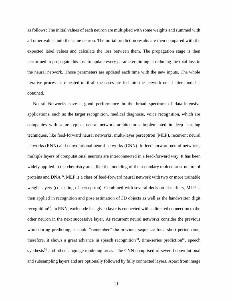
Neural Networks have a good performance in the broad spectrum of data-intensive
applications, such as the target recognition, medical diagnosis, voice recognition, which are
companies with some typical neural network architectures implemented in deep learning
techniques, like feed-forward neural networks, multi-layer perceptron (MLP), recurrent neural
networks (RNN) and convolutional neural networks (CNN). In feed-forward neural networks,
multiple layers of computational neurons are interconnected in a feed-forward way. It has been
widely applied in the chemistry area, like the modeling of the secondary molecular structure of
proteins and DNA66. MLP is a class of feed-forward neural network with two or more trainable
weight layers (consisting of perceptron). Combined with several decision classifiers, MLP is
then applied in recognition and pose estimation of 3D objects as well as the handwritten digit
recognition67. In RNN, each node in a given layer is connected with a directed connection to the
other neuron in the next successive layer. As recurrent neural networks consider the previous
word during predicting, it could “remember” the previous sequence for a short period time,
therefore, it shows a great advance in speech recognition68, time-series prediction69, speech
synthesis70 and other language modeling areas. The CNN comprised of several convolutional
and subsampling layers and are optionally followed by fully connected layers. Apart from image

12
recognition, CNNs have been successful in identifying faces71, objects 72 and traffic signs apart
from powering vision in self-driving cars73.
2.2.3 Convolutional Neural Network
The huge computational cost is a typical drawback in traditional neural networks, that is due
to the matrix multiplication operations involved massive parameters. CNNs easily tackle this
problem by introducing convolutions which make the local spatial coherence in the input ideal
for extracting relevant information with a lower computational cost.
The typical operations in CNN structure are introduced as follows:
a) Convolutional Step: a filter matrix is used to convolute with the original input matrix with
learnable kernels to get the ‘feature map’. Convolution preserves the spatial relationship
between pixels by learning image features using small squares of input data. By increasing the
number of filters, more matrix features can be extracted so that the network performs better in
recognizing patterns or classification to invisible matrices or images.
b) Activation Function: It is used to determine the outputs of the neural network by mapping
the resulting values to some certain range. As neural networks are used to implement complex
functions, sigmoid74, hyperbolic tangent (Tanh)75, rectified linear unit (ReLU)71 are the
commonly used non-linear activation functions. Both sigmoid and Tanh are saturating non-
linear functions where the output gradient decreases close to zero as the input increases.
Different from these two, ReLU is a non-saturating function, that the output returns 0 if it
receives negative input, otherwise the input will be returned. It can be written as 𝑓(𝑥) =
max (0, 𝑥). Previous works show that ReLU has become the default activation function for many

13
types of neural networks, as it greatly shortens the network converge period and improve
classification performance in deep neural network applications76, 77.
c) Pooling: Spatial Pooling (also called sub-sampling or down-sampling) summarizes feature
responses across neighboring pixels. It makes the feature dimension smaller so that the
computation load can be reduced, therefore, controls the overfitting problem. Besides, it helps
to retain the most important information.
d) Dropout: Dropout is that some units are chosen randomly to be abandoned during a
particular forward or backward pass. In the process of training, neuron interdependent learning
exists, which leads to the over-fitting problem. Dropout is a typical regularization method to
solve the problem by forcing a neural network to learn more robust features that are useful in
conjunction with many different random subsets of the other neurons.
Receptive fields, local connectivity, and shared weights are three structural characteristics in
CNN, which ensure the network to be robust enough for the shift, scale, and distortion variance
of the input data, as well as the noise. Normally, CNN is applied as a standard neural network
with some novel structures to tackle specific problems in various areas. H. Nam et al. used a
pre-trained CNN to obtain generic target representations from a set of labeled videos and applied
in visual tracking tasks78. Later, an automatic brain tumor segmentation method is proposed
which applied a novel two-pathway architecture to model both the local details and global
context and two CNNs are stacked to model local label dependencies. Even though the
distribution of the label is unbalanced, it can effectively solve medical segmentation problem79.
In NDE literature, P. Zhu et al. developed a CNN classification model with weighted loss
function in for eddy current testing defect detection with high classification result80. A novel
14
CNN model with ReLUs activation function is employed in the MFL response segments
classification81. The applied CNN model in this work is presented and explained in Chap 4.
2.3 Uncertainty Quantification
Quantification of uncertainties in models and measurements requires identification of sources
of error that lead to the uncertainties. The forward problem involves the use of a calibrated
model for probabilistic prediction, e.g., classification and segmentation, which has been widely
used in the computer vision, medical image and NDE fields82-85. This section will review
probabilistic modeling and variational inference, which is the foundations of derivations in the
Bayesian method, and the uncertainty sources in NDE area are clarified.
2.3.1 Probabilistic Modelling and Variational Inference
The uncertainty quantification tries to determine how likely certain outcomes are if some
aspects of the system are not exactly known. In Bayesian theory, the posterior distribution is
usually used to describe this relationship. Let 𝑋 = [𝑥𝑖]𝑖=1𝑁 ∈ 𝑅𝑑 be the training inputs and the
corresponding one-hot encoded categorical outputs 𝑌 = [𝑦𝑖]𝑖=1𝑁 ∈ [0,1]𝐾 , where 𝑁 is the
sample size, 𝑑 denotes the input variable dimension and 𝐾 is the number of categories. In the
Bayesian probabilistic modeling, posterior 𝑃(𝑤|𝑋, 𝑌) is computed over the weights 𝑤, which
captures the set of uncertainty model parameter vectors, given the data. The corresponding
posterior distribution can be expressed as:
𝑃(𝑤|𝑋, 𝑌) =𝑃(𝑌|𝑋, 𝑤)𝑃(𝑤)
𝑃(𝑌|𝑋) (6)

15
This distribution describes the most likely function based on the given information. Afterward,
the predictive distribution of the output for a new input point 𝑥∗ and a new output point 𝑦∗ can
be derived as:
𝑃(𝑦∗|𝑥∗, 𝑋, 𝑌) = ∫ 𝑃(𝑦∗|𝑥∗, 𝑤)𝑃(𝑤|𝑋, 𝑌)𝑑𝑤 (7)Ω
As the learning process of the posterior distribution is usually hard to evaluate analytically,
Radford M Neal investigated the Hamiltonian Monte Carlo, a Markov Chain Monte Carlo
(MCMC) sampling approach using Hamiltonian dynamics to approximate the posterior
distribution as calculated by Bayes Neural network86. The results consist of a set of posterior
samples without direct calculation but computationally complicated. Besides, the variational
inference method transforms the standard Bayesian learning from integration to optimization
problem. Tractable approximating variational distribution 𝑞𝜃(𝑤) indexed by a variational
parameter 𝜃, is applied to fit the posterior distribution 𝑃(𝑤|𝑋, 𝑌) that obtained from the original
model87, 88. The closeness to the optimal variational distribution and the posterior distribution is
measured by the Kullback–Leibler (KL) divergence, which is defined as
𝐾𝐿(𝑞𝜃(𝑤)||𝑃(𝑤|𝑋, 𝑌)), to find the optimal parameters 𝜃. Minimizing the Kullback–Leibler
divergence between 𝑞𝜃(𝑤) and 𝑃(𝑤|𝑋, 𝑌) is equivalent to maximizing the log evidence lower
bound,
𝐿 = ∫ 𝑞𝜃(𝑤)log P(𝑦|𝑥, 𝑤) 𝑑𝑤 − 𝐾𝐿((𝑞𝜃(𝑤)||𝑃(𝑤|𝑋, 𝑌)) (8)
with respect to the variational parameters 𝑞𝜃(𝑤). This is known as variational inference, a
general method applied in the Bayesian modeling.

16
2.3.2 Dropout as approximating variational inference
The uncertainty prediction in Neural Networks is accomplished by introducing Bayesian
inference methods for training recurring neural networks89 and convolutional network90, 91.
Several studies have demonstrated that Dropout92 and Gaussian Dropout 93applied before the
weighted layer can be used as approximating variational reasoning schemes in the deep
Gaussian process as they are marginalized over its covariance function parameters94.
Gal and Ghahramani implemented the dropout training in CNN as the Bayesian approximation
and developed the approximate variational inference in Bayesian NNs using Bernoulli
approximating variational distributions and relate this to dropout training95. In Neural Network,
normally the 𝐿2 regularization term is used to optimize the dropout process with weight decay
𝜆, resulting in a minimization objective:
𝐿𝑑𝑟𝑜𝑝𝑜𝑢𝑡 =1
𝑁∑ 𝐸(𝑦𝑖 , 𝑦��) +𝑁
𝑖=1 𝜆 ∑ (||𝑊𝑖||22+ ||𝑏𝑖||2
2)𝐿
𝑖=1 (9)
where 𝑦�� is the output with L layers in the network. 𝐸(. , . ) represents the loss function, such as
the softmax loss or the Euclidean loss (squared loss) with weighted matrices 𝑊 and bias vector
𝑏 . In the Bayesian Neural Networks with dropout, the tractable approximating variational
distribution 𝑞(𝑊𝑖) for every layer is defined as:
𝑊𝑖 = 𝑀𝑖 ∗ 𝑑𝑖𝑎𝑔 ([𝑧𝑖,𝑗]𝑗=1
𝐾𝑖) (10)
Here 𝑧𝑖,𝑗are Bernoulli distributed random variables with some probabilities𝑝𝑖 , and 𝑀𝑖 are
variational parameters need to be optimized. As the variational inference defined in the last
section cannot be evaluated analytically for approximating distribution, an unbiased estimator
to 𝐿 is proposed as:

17
�� =1
𝑁∑ 𝐸 (𝑦𝑖 , 𝑓(𝑥𝑖,��𝑖)) −𝑁
𝑖=1 𝐾𝐿((𝑞(𝑤)||𝑃(𝑤|𝑋, 𝑌)) (11)
The softmax loss is applied to normalize the network predictions, which are interpreted as
probabilities. As sampling from 𝑞(𝑊𝑖) is identical to performing dropout operation in a network.
The second term in eq.8 can be approximated as ∑ (𝑝𝑖𝑙
2
2||𝑊𝑖||2
2 +𝑙2
2||𝑏𝑖||2
2)𝐿𝑖=1 with prior length
scale 𝑙 which is derived in the previous work96. With the Monte Carlo integration, the
approximating predictive posterior distribution can be rewritten as 𝑃(𝑦∗|𝑥∗, 𝑋, 𝑌) ≈
1
𝑇∑ 𝑝(𝑦∗|𝑥∗, ��𝑖))
𝑇𝑡=1 . Therefore, it has proven that 𝐿 is an approximation to 𝐿𝑑𝑟𝑜𝑝𝑜𝑢𝑡, resulting
dropout is the approximating variational inference in Bayesian NNs.
2.3.3 Source of Uncertainties
In general, the sources of uncertainty in the context of modeling, based on the character of
uncertainties, can be categorized as:
• Aleatoric uncertainty: the intrinsic randomness of a phenomenon.
• Epistemic uncertainty: the reducible uncertainty caused by lack of knowledge.
However, in most cases, it is difficult to determine the uncertainty category in a more general
way, which should depend on the specific context and application23. In the Bayesian methods
that are applied in Neural Network, epistemic uncertainty is modeled by placing a prior
distribution over a model’s weights and then trying to capture how much these weights vary
given some data while aleatoric uncertainty, on the other hand, is modeled by placing a
distribution over the output of the model. Epistemic uncertainty, often referred to model
uncertainty, accounts for uncertainty in the parameters of the machine learning model which
could be improved by given enough data. On the other hand, aleatoric uncertainty captures

18
inherent noise in the data, such as sensor noise or motion noise, resulting in uncertainty which
cannot be reduced even if more data were to be collected. Normally, aleatoric uncertainty can
be categorized into homoscedastic uncertainty, which assumes identical observation noise for
every input, and heteroscedastic uncertainty where different extents of noise for each input97.
Generally, in NDE area, the data are generated by the physics model based on the selected
defect parameters, material properties, etc., and then passed through the machine learning model
to obtain the output. The final predicted outputs are collected to estimate the uncertainties
brought by data and the machine learning model. The flow diagram of the whole process is
shown in Fig 2.2.
Figure 2. 2 The flow diagram of the entire NDE UQ system
In this thesis work, the uncertainty quantification to MFL is based on the Bayesian inference
method. According to the previous definitions, the uncertainties could be divided into the data
related and the machine learning model-related uncertainties, while the former can be
understood as the aleatoric uncertainty and the latter as the epistemic uncertainty. In this case,
data are generated from the physical model, thus the inherent noise in data is considered as

19
coming from the physics model. In the Bayesian approach, only the uncertainties directly related
to data and model are taken into consideration, the specific uncertainty quantification to this
physical model needs further investigation.
To be specific, the sources of aleatoric uncertainties are physics properties, data-producing
method, and noise:
• Physics properties: piping material properties such as grain size, fracture toughness, chemical
composition, yield strength, and ultimate tensile strength; loading/pressure, e.g., operating
pressure; geometry such as outer diameter, thickness, defect shape, size, and location.
• Data producing method: the data can be collected from the real field testing/experiments or
simulation platforms, like ANSYS, ANSOFT, and COMSOL. Even with the same experiment
settings, different software results may vary from each other. In this work, ANSYS is adopted
to generate MFL data.
• Noise: experimental device may have various measurement noise to contaminate measured
signals, i.e., sensor lift-off variation noise, that the distance between the pipe wall and the
detector sensors always varies throughout the whole detection process due to the surface
discontinuity and vibration of the detector98; seamless pipe noise, which contributes to a helical
variation in the grain properties of the seamless pipe99; system noise, which is referred as
inherent noise in on-board electronics100. During the experiment, these noises can be modeled
as additive white Gaussian noise in the data, which presented most of the high-frequency
noise101.
The sources of epistemic uncertainties are related to the model structure and hyperparameters:
• Model structure: Different applying NNs bring uncertainties to the whole process. In this
thesis work, only CNN is implemented as the machine learning model.

20
• Hyperparameters: uncertainties are from various parameters and functions in the model, for
example in CNN, differences in the number of convolutional layers, kinds of activation
functions and loss functions will bring uncertainties.
Figure 2. 3 The diagram of NDE uncertainties
Fig 2.3 shows the diagram of the NDE uncertainties and their sources for this study.
According to the analysis above, the uncertainties are involved from multiple sources. In this
MFL defect classification work, the variation in defect shape, size, location, noise and data
amount are considered as the main sources and their influences on defect detection will be
explicitly investigated in Chap 5.

21
Chapter 3: Magnetic Flux Leakage Simulation
3.1 Finite Element Modeling
Three-dimensional (3-D) finite element method (FEM) is a widely adopted approach in
analyzing and modeling the accurate 3-D defects and detailed MFL signals102. 3-D FEM has
been used as a general discretization technique for many physical problems in various
engineering fields, such as structure analysis, heat transfer, fluid flow, electromagnetic potential.
In a structural simulation, FEM helps to predict the deformation of a structure and providing
stiffness and strength visualizations103. R. W. Lewis et al. applied an adaptive finite element
analysis (FEA) with an error estimation technique in heat conduction problem and provided
satisfactory results for non-linear transient heat diffusion problems and steady incompressible
flow problems104. FEM also provides an effective solution to the 3D electromagnetic forward-
modeling problem in the frequency domain accompanied vector and scalar potentials and
unstructured grids105.
The physical interpretation of FEM is to subdivide the mathematical model into disjoint (non-
overlapping) components called finite elements of simple geometry. The degrees of freedom are
used to represent the response of each element, which is characterized by the value of an
unknown function or function at a set of nodes106. In general, the number of degrees of freedom
equals to the product of the number of nodes and the number of values of the field variables,
possibly their derivatives, that must be calculated at each node. The analytical solution at each
element is converted to solve the boundary value problems for differential algebraical equations
at selected elements. All elements are then assembled to form a discrete model in terms of a
system of equations, which is an approximation to the original mathematical model. The

22
variational methods are used to approximate a solution by minimizing an associated error
function.
In 3-D finite element computation of MFL numerical models, the geometry is constructed with
the specified material properties and boundary conditions. It is then discretized into small
regions which create the equations to be solved. As discussed in Chap 2, the simplified
Maxwell’s equations could describe the electromagnetic phenomena in MFL with permanent-
magnet excitation. Based on Maxwell’s theory accompanied by eq.1 and eq.3 in Chap 2:
∇ × 𝐴 = �� (12)
∇ ×1
𝜇∇ × 𝐴 = 𝐽 (13)
where A is the vector magnetic potential vector, B is the magnetic flux density vector, μ is the
spatial permeability107. In the finite element model, the equations can be expressed as108:
[𝐾]𝐴 = 𝑆 (14)
where [𝐾] is a global stiff matrix, 𝐴 is an unknown column vector about magnetic vector
potential and S is a column vector of the excitation source. With proper boundary conditions,
the magnetic potential vector 𝐴 can be solved from this formula and the distribution of magnetic
flux density is then obtained. As FEM is usually used in MFL signals analysis by correlating
MFL signals and the defect geometry parameter, in this work, ANSYS finite element software
is used to obtain the three-dimensional MFL signals.
3.2 Simulation Environment
The 3-D model defines the simulation geometry in ANSYS, shown in Fig 3.1. The defects are
set to locate in the center area of the specimen, while the size of the specimen is of 400 mm long,

23
200 mm width and 10 mm thick. The depth of the defect is set to be 5 mm, 8 mm, and 10 mm.
In other words, the flaw depth is of 50%, 80% and 100% to the sample. The York, magnets,
brushes and the specimen compose the whole MFL 3-D finite element simulation model. The
permanent magnets work as the magnetic flux induction to activate the magnetic circuit, and also
are load. Brushes act as a transmitter of magnetic flux from the tool into the piping material, and
strategically placed tri-axial Hall effect sensor heads can accurately measure the 3-D MFL vector
fields. In ANSYS, the chosen permanent magnets, are translated into equivalent current and
apply on every element and node of the model102. The material of magnet is NdFe30, and that of
York and brushes are all nickel, while the specimen is made with iron. Huang et al. proved that
the MFL peak to peak value is inversely proportional to the lift-off value9. In order to obtain a
precise result in the experiment, a 20 mm 𝑋 20 mm measured area is selected around the center
of the specimen with 1 mm lift-off to receive the output MFL signals.
Figure 3. 1 3D model geometry of MFL inspection in ANSYS
24
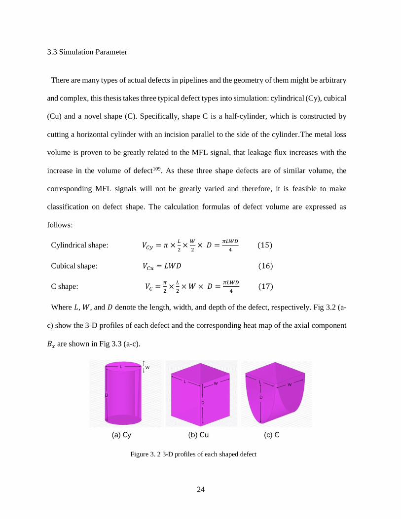
3.3 Simulation Parameter
There are many types of actual defects in pipelines and the geometry of them might be arbitrary
and complex, this thesis takes three typical defect types into simulation: cylindrical (Cy), cubical
(Cu) and a novel shape (C). Specifically, shape C is a half-cylinder, which is constructed by
cutting a horizontal cylinder with an incision parallel to the side of the cylinder. The metal loss
volume is proven to be greatly related to the MFL signal, that leakage flux increases with the
increase in the volume of defect109. As these three shape defects are of similar volume, the
corresponding MFL signals will not be greatly varied and therefore, it is feasible to make
classification on defect shape. The calculation formulas of defect volume are expressed as
follows:
Cylindrical shape: 𝑉𝐶𝑦 = 𝜋 ×𝐿
2×
𝑊
2× 𝐷 =
𝜋𝐿𝑊𝐷
4 (15)
Cubical shape: 𝑉𝐶𝑢 = 𝐿𝑊𝐷 (16)
C shape: 𝑉𝐶 =𝜋
2×
𝐿
2× 𝑊 × 𝐷 =
𝜋𝐿𝑊𝐷
4 (17)
Where 𝐿, 𝑊, and 𝐷 denote the length, width, and depth of the defect, respectively. Fig 3.2 (a-
c) show the 3-D profiles of each defect and the corresponding heat map of the axial component
𝐵𝑥 are shown in Fig 3.3 (a-c).
Figure 3. 2 3-D profiles of each shaped defect

25
Figure 3. 3 𝐵𝑥 component of each shaped defect (L, W, D = 5mm)
For each shape defect, different length, width, and depth are assigned and combined together
to enrich the dataset, which will be applied in the CNN to classify the defect shape and size. The
specific defect parameters are explained in Table 3.1 and it can be seen that there are 27 kinds
of size defects under each shape and totally, 81 kinds of defects are simulated to achieve a
balanced dataset. In one simulation, the acquired axial, tangential and radial component signals
are referred to a group of MFL signals and there will be three groups of MFL signals of every
defect. Generally, 243 groups of MFL signals are simulated, while 170 groups are used as the
training data and the others are the test data in defect classification tasks.
Table 3. 1 MFL simulation defect parameters
Cy Cu C
Length 5mm/8mm/10mm 5mm/8mm/10mm 5mm/8mm/10mm
Width 5mm/8mm/10mm 5mm/8mm/10mm 5mm/8mm/10mm
Depth 5mm/8mm/10mm 5mm/8mm/10mm 5mm/8mm/10mm

26
Chapter 4: Convolutional Neural Network in NDE
4.1 Proposed CNN model
In general, the Convolutional Neural Network is considered as a hierarchical feature extractor,
which extracts features of different abstract levels and maps the input image or matrix into a
feature vector by several fully connected layers. The overall architecture and detailed settings
of the proposed network are illustrated in Fig 4.1. All convolutional filter kernel elements are
trained from the data in a supervised fashion by learning from the labeled MFL data.
Figure 4. 1 The proposed CNN architecture
In the proposed architecture, four convolutional layers are employed and each of them is
activated by ReLU, which enable the network to extract the important features of the input. The
first two convolutional layers with 32 kernels of 3 × 3 sized filters to obtain the corresponding
feature maps of the input matrix. The number of kernels is selected according to the principle

27
that keeps the total number of activations (number of feature maps times number of pixel
positions) to be non-decreasing from one layer to the next. Maxpooling layer takes the largest
element from each feature maps within the 2x2 window, which helps to reduces the
dimensionality of our feature map. These two connected convolutions with a pooling layer act
as the feature extractors from the input and in this case, produce 32 feature maps. Then 25% of
neurons are dropout to increase the validation accuracy and decrease the loss initially before the
trend starts to go down.
The previous layers are employed again to deeper the network and therefore, more detailed
features of the input image or matrix can be extracted. As the output of previous layers
represents high-level features of the input image, a fully connected layer is added to combine
features to create a model. Finally, the softmax activation function is applied to classify the
inputs into various classes. It is a widely applied function in various multiclass classification
methods by taking a vector of arbitrary real-valued scores and squashing the feature maps to a
vector of values that sum to one110, 111. In this way, the output probability distribution over
predicted output classes can be specified. All parameters are jointly optimized through
minimization of the misclassification error over the training process. The entire experiment was
implemented on the Google Cloud high-performance computing platform, with 8 virtual CPUs
and an NVIDIA Tesla K80 as computing resources. The project is based on Keras and
Tensorflow neural networks libraries. The performance of the proposed CNN will be validated
on some other NDE applications and the simulated MFL detection data, which will be shown in
the following two sections.

28
4.2 Validation of the proposed CNN in other NDE application
In order to validate the generality and robustness of the proposed network, three different NDE
related datasets are tested in the proposed CNN and some of the results are compared with
previously published work. The comparison results showed that the proposed CNN is effective
in solving different defect detection and recognition problems in NDE area.
4.2.1 Concrete Crack Detection
In transportation infrastructure maintenance, automatic detection of pavement cracks is an
important task for driving safety assurance. The objective of the crack detection problem is to
determine whether a specific pixel in pavement images can be classified and grouped as a crack.
Zhang et al. used a supervised deep convolutional neural network to detect the crack in each
image patch and compared the classification performances with other two conventional machine
learning methods: Support Vector Machine and the Boosting method. The results showed that
compared with CNNs, SVM and boosting method cannot correctly distinguish the crack from
the background112. Inspired by this, my proposed CNN is trained to classify image patch from
the open-sourced concrete images.
458 high-resolution concrete surface images with various cracks are collected from various
Middle East Technical University (METU) campus buildings113. Following the sampling
methods proposed in 112, 40000 annotated RGB images with 227 x 227 pixels are generated and
are divided into two classes as negative and positive crack images. The numbers of crack and
non-crack patches are set to equal in this dataset. Fig 4.2 shows sample images with crack and
without crack.

29
Figure 4. 2 Concrete image with crack (left) and without crack (right)
Noted that the number of background patches is far more than that of crack patches in an
image, the accuracy calculated in CNN may overestimate the possibility of crack. Therefore, the
precision (P), recall (R) and F1 score are applied as performance criteria, which defined as
follows:
𝑃 =𝑡𝑟𝑢𝑒 𝑝𝑜𝑠𝑖𝑡𝑖𝑣𝑒
𝑡𝑟𝑢𝑒 𝑝𝑜𝑠𝑖𝑡𝑖𝑣𝑒 + 𝑓𝑎𝑙𝑠𝑒 𝑝𝑜𝑠𝑖𝑡𝑖𝑣𝑒
𝑅 =𝑡𝑟𝑢𝑒 𝑝𝑜𝑠𝑖𝑡𝑖𝑣𝑒
𝑡𝑟𝑢𝑒 𝑝𝑜𝑠𝑖𝑡𝑖𝑣𝑒 + 𝑓𝑎𝑙𝑠𝑒 𝑛𝑒𝑔𝑎𝑡𝑖𝑣𝑒
𝐹1 =2𝑃𝑅
𝑃 + 𝑅
Table 4.1 shows the performance of the proposed CNN in this concrete crack classification task.
It can be seen that CNN can learn the deep features from the concrete crack images and the cracks
can be distinguished from the backgrounds with high accuracy.
Table 4. 1 Comparison result in Concrete Crack Data
Method Precision Recall F1 Score
Proposed CNN 0.9987 0.9967 0.9971

30
4.2.2 Surface Defect Detection
The inspection to the steel surface is an important research area114, 115 and a surface defect
database, constructed by Northeastern University (NEU), has been applied in feature extraction
methods for defect recognition116-118. In this database, six kinds of typical surface defects of the
hot-rolled steel strip are collected, i.e., rolled-in scale (RS), patches (Pa), crazing (Cr), pitted
surface (PS), inclusion (In) and scratches (Sc). The database includes 1,800 grayscale images,
where each typical surface defect has 300 samples. Fig 4.3 shows the sample images of six kinds
of typical surface defects. Each image consists of 200 × 200 pixels. In this NEU surface
database, both the intra-class defects of one type and the inter-class defects exist large differences
in appearance. For instance, there are horizontal, vertical and slanting scratches among the Sc
surface defects while RS, Cr, and PS typed defects are varied. Besides, the changes in
illumination and material influence the defect images.
Figure 4. 3 NEU surface defect sample image

31
In surface inspection, a large amount of training dataset is obtained which is costly for feature
extraction. Therefore, Ren et al. utilized a pre-trained deep learning network: Decaf119 to extract
patch features from input images and multinomial logistic regression (MLR) classifier is chosen
to generate the defect heat map based on patch features, and predicted the defect area by
thresholding and segmenting the heat map117. Decaf is previously trained on the ImageNet
challenge to predict 1000 classes of objects and its weights and model structure are reused as the
feature extractor to the small data in another domain120-122. Comparison results of the proposed
model and other benchmark methods are shown in Fig 4.4:
Figure 4. 4 Comparison model accuracy in reference work117

32
Figure 4. 5 Model accuracy of the proposed network
The results in Fig 4.4 indicated that the proposed Decaf model with MLR classifier provided
the highest accuracy: 99.27% and in Fig 4.5, the classification accuracy of my proposed CNN
can reach up to 99.30% within 500 epochs. Although training CNN requires a large amount of
time, it shows great performance in classifying surface defects on this NEU dataset. In dealing
with image classification problems, it is common to use a deep learning model pre-trained for a
large and challenging image classification task, but the choice of the appropriate source data or
source model is an open problem.
4.2.3 Defect Detection on Eddy Current Testing
Eddy Current Testing (ECT) is another typical electromagnetic testing method in NDE to
detect and characterize defects in conductive materials. The electromagnetic induction is used to
produce the alternating current and perturbations in the induced eddy current indicate the
presence of defects80. An eddy current testing dataset, obtained from EPRI (Electric Power
Research Institute, USA), consists of multi-frequency ECT data from inspection of 37 steam

33
generator (SG) tubes using array probes under four frequencies, i.e., 70 kHz, 250 kHz, 450 kHz,
and 650 kHz123. In previous work, robust principal component analysis (RPCA) is utilized to
preprocess the initial data to detect and enhance the potential flaw region, referred as the region
of interests (ROIs), and separate the background. Fig 4.6 shows an example of segmented initial
image samples and its sparse component with enhanced defect area (ROIs) and suppressed
background. Then subsampling is performed to divide the individual raw image into 374 defect
images and 374 non-defect images and each of them is of 32 × 200 pixels. Among the total 748
sample images, 648 are used for training the CNN model while the others are used for testing the
performance80.
Figure 4. 6 One initial ECT sample image (left) and its sparse component with ROIs (right)
In the reference work80, a classical CNN structure with a proper weighted loss function is
adopted by applying larger weight of errors resulted from defect samples to improve the
performance of their CNN model. A five-fold validation technique is implemented to verify the
network by setting different threshold values. Five training datasets are used separately to train
five CNN models and the results showed 𝜆6 dataset is of higher accuracy, shown in Fig 4.7. From
the reference result plot, the x-axis represents the threshold 𝜃 which is involved in assigning
penalty in the proposed weighted loss function. When 𝜃 is 0.5, either the defect or the non-defect

34
images are of the same penalty. The performance of the proposed CNN trained on this ECT
datasets with threshold 𝜃 = 0.5 and no weighted loss function are shown in Fig 4.8.
Figure 4. 7 Comparison model accuracy in reference work80
Figure 4. 8 Example model accuracy and model loss of the proposed network

35
The above graphs show that the accuracy in both networks is quite good when assigning no
penalty to the defect and non-defect ECT images. My proposed CNN is a little unstable in
convergence, which is because the network is not specifically finetuned on this ECT defect
classification tasks. However, its high classification accuracies prove that the defect area in ECT
images can be distinguished from the background, in other words, the versatility of the proposed
CNN is addressed.
4.3 CNN Classification Result in MFL
The simulated MFL signals described in Chap.3 are trained and tested in the proposed CNN,
and each CNN model for different MFL classification tasks converges within 150 epochs. In
different classification tasks, the MFL signals are assigned with corresponding labels. To be
specific, Cu, Cy, and C are marked in the defect shape classification task, while 5mm, 8mm,
and 10mm are marked in the defect size classification task. Each group of MFL signals consists
of three 81 × 81 sized matrices, representing the axial, tangential and radial components,
respectively. Similar to how RGB images are processed, these three MFL matrices are stacked
together to be passed through CNN. After a series of convolution, pooling and dropout
operations, the MFL defect features can be extracted and combined to make the classification
and the results will be discussed as follows:
Experiment 1: Defect shape and size classification tasks to MFL data in proposed CNN model.

36
Table 4. 2 Classification accuracy for MFL signals
Accuracy Shape Length Width Depth
Proposed CNN 100% 97.26% 95.89% 94.53%
From Table 4.2, it can be seen that the proposed network has shown superior performances in
shape and size classification task for MFL signal data, especially when classifying different
defect shapes. Among the defect size classification, depth is the “hardest” one to deal with. The
main characteristics of defect depth are represented from the axial peak and vale values of
magnetic leakage field, which will also be affected by length and width15. Although CNNs are
most commonly applied in visual imagery, in this case, the essential defect shape and size
features can still be learned from 3-D MFL signals with high classification accuracy.
Experiment 2: CNN performance on distorted MFL data
During the MFL defect detection, various measurement noise such as mechanical vibrations,
velocity effect, sensor lift-off variation, etc., greatly distorted MFL signals. To simulate this
noise-degraded MFL data generation, Gaussian noise is generated to contaminate the MFL
signals and its probability density function 𝑝 is:
𝑝 =1
𝜎√2𝜋𝑒
−(𝑥−𝜇)2
2𝜎2 (18)
where 𝑥 represents the Gaussian noise level, 𝜇 and 𝜎2 represents the mean value and variance.
In this case, different percentage of signal points among each group of MFL matrices are
randomly assigned with the additive Gaussian noise with the mean value of 0.005 and variance
of 0.001. Therefore, each new noisy MFL signal point 𝑑𝑖𝑛 can be expressed as:
𝑑𝑖𝑛 = 𝑑𝑖 + 𝑥𝑖 , 𝑖 ∈ [0, 𝜖 × 19682] (19)

37
Where 𝜖 represent how much points is randomly selected among the 3-D MFL matrices to add
noise and 𝑖 is the specific chosen position, where each matrix composed of 6561 points. 𝑑𝑖 and
𝑥𝑖 are the original MFL signal point and gaussian noise point. Three noisy MFL datasets are
generated by setting 𝜖 equals to 1%, 5%, and 10% respectively, which are then put into the
proposed CNN to figure out how noisy MFL data affect the defect shape and size classification
accuracy.
Besides, during the MFL testing, the variation in defect location changes the measured
magnetic field as well. To simulate this variance, different amounts of defects described in
Chap3, are selected to be moved randomly away from the previous places (center of the
measured area). Their new locations are set within 5mm from the previous spot, while the
measurement area is fixed. Among the whole MFL data, 5%, 10%, 15%, and 20% defects are
evenly chosen to be randomly relocated, respectively, and then, four new MFL defect datasets
with location variation are generated. The relationship between the altered defect location and
the defect classification performance of the proposed network can be found by putting these
four MFL datasets into CNN respectively and following the same training and testing process
in the previous section. Fig 4.9 presents examples of two groups of magnetic fields affected by
different defect positions. Defect in the first row is placed on the left side of the original position,
while the defect in the second row is on the lower right side.

38
Figure 4. 9 Magnetic fields corresponding to different located defect.
The variation in data increases the difficulty of the applied classification technique but in
another aspect, represents this CNN’s robustness in MFL inspection. The comparative accuracy
results are shown in Fig 4.10 and Fig 4.11.

39
Figure 4. 10 Noise influence on different defect classification tasks
40
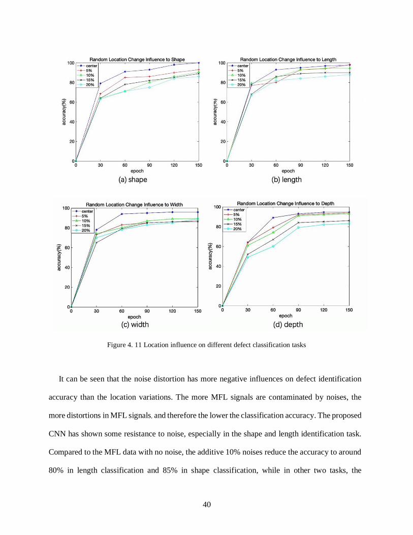
Figure 4. 11 Location influence on different defect classification tasks
It can be seen that the noise distortion has more negative influences on defect identification
accuracy than the location variations. The more MFL signals are contaminated by noises, the
more distortions in MFL signals, and therefore the lower the classification accuracy. The proposed
CNN has shown some resistance to noise, especially in the shape and length identification task.
Compared to the MFL data with no noise, the additive 10% noises reduce the accuracy to around
80% in length classification and 85% in shape classification, while in other two tasks, the
41
classification accuracies fell almost by half. The variation in defect location affect the CNN’s
performance, but the influence is quite small when compared with noise. It can be seen that, when
20% of defects are relocated, the variation in accuracies is less than 20% compared to the result
of original MFL data. Therefore, the proposed defect identification network has good robustness
in position variance and noise distortions.
4.4 Comparison with Other Machine Learning Methods
In previous works, feature-based techniques are proposed to accomplish the defect
identification in MFL measurements22, 45, 47. Support vector machine (SVM) and tree-based
techniques, e.g., decision tree (DT), are also popular tools in building the prediction models and
solving the classification and regression problem 124-127. SVM is based on the statistical learning
theory while DT is built following a multistage or hierarchical decision scheme. They have both
shown great advances in multiple areas: an alternative procedure to the Fisher kernel is used in
SVM and applied in the multimedia classification task128; Y. Bazi and F. Melgani designed an
optimal SVM classification system for hyperspectral imagery129. P. Ye applied the DT on the
visual expression identification and it shows comprehensive and accurate recognition results130.
In this section, the principle of those two methods is introduced and used as the direct inversion
models to present the comparison results with the proposed algorithms in this thesis on the MFL
simulation data.
42
4.4.1 Support Vector Machine
Similar to neural networks, Support Vector Machine (SVM) is one of the powerful kernel-
based learning algorithms that analyze data for classification and regression. When the input
data is not linearly separable, the non-linear SVM transforms the input space into a high-
dimensional output space. Different distributions in the feature space could fit a linear
hypersurface to separate all samples into the classes131. This transformation can be performed
by kernel function which allows more simplified representations of the data, such as polynomial,
sigmoidal, and Gaussian (RBF)132-134. The various regularization algorithms and the kernel
functions enable SVM to have better performance in generalization and reduce the risk of over-
fitting based on the rigorous statistical learning theory. In MFL defect detection area, SVM has
proven to be an effective technique in the reconstruction of defects shape features in 48, while a
least-square SVM model is used to correlate the physics-based geometric and feature parameters
to realize a fast reconstruction of 3-D defect profiles135.
The main idea behind SVM is to find a hyperplane that can correctly separate the sample data
points. Given the input data points 𝑥𝑖 and the corresponding class label 𝑦𝑖 , the classifying
hyperplane is constructed as:
𝑤𝑇𝜑(𝑥) + 𝑏 = 0 (20)
where 𝜑(∙)is a non-linear function and similar to neural networks, this function maps the input
space to a high, possibly infinite, dimensional feature space. The boundary condition should
satisfy:
𝑦𝑖[𝑤𝑇𝜑(𝑥𝑖) + 𝑏] ≥ 𝛾, 𝑖 = 1, … , 𝑁 (21)

43
The optimization problem is then transferred to choose weights 𝑤 and bias 𝑏, and select the
proper kernel functions.
SVM performs well when dealing with evenly unstructured and semi-structured data with low
overfitting risk and high generalization136-138. However, it is quite difficult to choose a perfect
kernel function. In multi-class classification problems, it needs a long training period, so their
training on a large dataset is still a bottleneck.
4.4.2 Decision Tree
Decision Tree (DT) is another widely used supervised machine learning technique by building
a classification or regression models in the form of a tree-like structure139. The final result is a
tree with decision nodes and leaf nodes. Decision nodes represent where the data to be split and
each leaf node represents a class label or a decision. The complexity of the decision rules
increases along with the depth of the tree. DT can learn from the data to approximate a sinusoid
function based on specific decision rules. Unlike the black-box algorithms, e.g., SVM and NN,
DT interprets the data by following a strict logic. It is a non-parametric method without the
assumption of the distribution of the data and the structure of the real model140. The steps
involved in the DT construction process are splitting, pruning and selecting the tree.
a) Splitting: The decision tree is built by dividing training data into smaller subsets repeatedly
according to predictor variables.
b) Pruning: To avoid the extra calculation in the searching process, branches of the tree are
shortened by converting some branch nodes to leaf nodes and deleting the leaf nodes under the
original branch. It is an effective strategy to solve the overfitting problem.

44
c) Selecting Tree: It is the process of finding the smallest and the most efficient tree to fit the
data according to various decision rules. Normally the lowest cross-validated error is set as the
evaluation index.
In the NDT area, DT approach is commonly applied as the comparison feature-based network
to provide comparable results. D'Angelo and Rampone proposed a content-based image retrieval
(CBIR) solution to classify the aerospace structure defects detected by eddy current non-
destructive testing and the J48 Decision Tree are used to evaluate the proposed system’s
performance in defect recognition141. Later, DT and other feature-based networks are used to
compare with the proposed neural networks in MFL defect detection task22. In general, Decision
Tree is easy to understand and is considered as the fastest way to identify the most significant
variables and the relation between the variables. However, in multi-class problems, the
probability of overfitting is relatively high and prediction accuracy is low.
4.4.3 Comparison Results
In MFL defect detection task, the proposed CNN network is compared with two feature-based
machine learning models: SVM and Decision Tree. SVM is trained with the Sigmoid kernel, while
in DT, ID3 (Iterative Dichotomiser 3) algorithm is used to generate the tree.
Table 4. 3 Network comparison result in MFL
Accuracy Shape Length Width Depth
Proposed CNN 100% 97.26% 95.89% 94.53%
SVM 65.75% 71.23% 83.56% 89.04%
Decision Tree 90.41% 87.67% 93.15% 86.30%

45
The comparative results are presented in Table 4.3. The accuracy of the proposed CNN is much
better than the other models. In this simulated MFL defect dataset, there exist data variations in
each classification task. Take the shape detection, for example, although there are 81 groups of
MFL signals under each label, the corresponding defect size are not fixed. To SVM and DT, the
extracted features are sensitive to variation in data, especially for small defects; however, CNN
can suppress the adverse interference of this variation and therefore, outperformance in pinpointing
the distinguishing features of MFL signals.

46
Chapter 5: Uncertainty Estimation in MFL NDE
Based on the discussion in section 2.3, this chapter explicitly explains how the Bayesian
variance inference applied in CNN to obtain the aleatoric and epistemic uncertainties, which is
proposed by the reference work142. Then this uncertainty estimation approach is applied in my
proposed CNN to MFL defect detection, which helps to explain the relationship between data
and model variation and aleatoric and epistemic uncertainties
5.1 Aleatoric Uncertainty and Epistemic Uncertainty in CNN
In the neural network, as explained before in section 2.3, the dropout result is of Gaussian
distributions 𝒩(𝑤|𝜇, 𝜎2), where 𝑞𝜃(𝑤) are learned with the training dataset. Since most of the
classification problems are discrete and finite, with the Monte Carlo integration, the
approximating variational predictive posterior distribution can be constructed as:
𝑞��(𝑦∗|𝑥∗) =
1
𝑇∑𝑃(𝑦∗|𝑥∗, ��𝑡) (22)
𝑇
𝑡=1
where 𝜃 is the optimized variational parameter to minimize eq.8 and T is the number of samples
are set to obtain the distribution, [��𝑡]𝑡=1𝑇 are the realized weight vectors derived from variational
distribution. 𝑥∗ and 𝑦∗ represent the new input and corresponding one hot encode output. As there
is no explicit function between the categorical result and Gaussian distributions, the variance of
the variational predictive distribution allows us to evaluate how much the model is confident in
its prediction, that is to say, the uncertainty can be quantified. According to the definition, the
variance is given by
𝑉𝑎𝑟𝑞��(𝑦∗) = 𝐸𝑞��
(𝑦∗⊗2) − 𝐸𝑞��(𝑦∗)⊗2 (23)

47
Based on a variant of law of the total variance, eq.23 can be derived as142:
𝑉𝑎𝑟𝑞��(𝑦∗) = ∫[𝑑𝑖𝑎𝑔(𝐸𝑝[𝑦
∗]) − 𝐸𝑝[𝑦∗]𝐸𝑝[𝑦
∗]𝑇]𝑞��(𝑤|𝑋, 𝑌)𝑑𝑤
+∫(𝐸𝑝[𝑦∗] − 𝐸𝑞[𝑦
∗]) (𝐸𝑝[𝑦∗] − 𝐸𝑞[𝑦
∗])𝑇𝑞��(𝑤|𝑋, 𝑌)𝑑𝑤
= 𝐸[𝑑𝑖𝑎𝑔(𝑝(𝑤)) − 𝑝(𝑤)⊗2] + 𝐸[𝑝(𝑤) − 𝐸(𝑝(𝑤))]⊗2 (24)
𝑑𝑖𝑎𝑔(𝑣) is a diagonal matrix with the element of the vector 𝑣 and 𝑥⊗2 = 𝑥𝑥𝑇 . 𝑝(𝑤) =
𝑠𝑜𝑓𝑡𝑚𝑎𝑥(𝑓𝑤(𝑥∗)), where a new output 𝑦∗is made for a given input 𝑥∗, different features are
generated with randomly assigned 𝑤 , and each feature is weighted differently to produce the
posterior distribution. The first term in eq.24 is defined as the aleatoric uncertainty as its
expectation is over 𝑞��(𝑤), which captures the inherent randomness of an output. The second term
in eq.24 is epistemic uncertainty as its expectation is only related to the network weight parameter
𝑤, which is related to the model only. To estimate uncertainties in CNN classification task, based
on the previous derivation, Kwon defined the predictive uncertainty estimators as:
Aleatoric: 1
𝑇∑ 𝑑𝑖𝑎𝑔(��𝑡) − ��𝑡
⨂2𝑇𝑡=1 (25)
Epistemic: 1
𝑇∑ (��𝑡 − ��)⨂2𝑇
𝑡=1 (26)
where ��𝑡 = 𝑠𝑜𝑓𝑡𝑚𝑎𝑥(𝑓𝑤(𝑥∗)) and �� =1
𝑇∑ ��𝑡
𝑇𝑡=1 . With increasing T, the summation of these
two terms converges in probability to eq.24142. Each output element of softmax function has a
certain probability and consist to a vector, thus the variability of the predictive distribution can
be obtained by T times calculations.
To be more specific, in aleatoric uncertainty estimator, the diagonal matrix of expected output
𝑦∗ is subtracted by the inner product of the softmax-generated vectors. This operation is repeated
T times and then being averaged by T to make it tractable. The variability of the output is

48
considered to be from the inherent noise in data., therefore, the aleatoric uncertainty is
considered to be related to the data variation. In the MFL inspection, this variance is from the
physical model which generated the simulated MFL signals. In the epistemic estimator, based
on the variational distribution 𝑞(𝑦∗|𝑥∗), the expected outcome 𝑦∗ is represented by the average
of the softmax-generated vectors of T samples. Then this average is subtracted from the softmax-
generated output. Afterward, for each element, the subtraction is multiplied by its transpose and
the summation of the output matrix make the process tractable. As the variability of the output
coming from the model, referred as the proposed CNN model in this thesis, the epistemic
uncertainty is considered to capture the model variation and is not proportional to the validation
accuracy. In this way, the underlying distribution of the outcome can describe the inherent
variability of data and model and has numerical stability as well.
5.2 Uncertainty Estimation on MFL
5.2.1 Uncertainty estimation in the proposed CNN on MFL
The proposed uncertainty quantification method142 has performed well in ischemic stroke
lesion segmentation task by providing additional assistance to a more informed decision.
Inspired by this, I involved the predictive estimator (eq.26 and eq.27) and utilized the various
outputs of a Dropout function to define a distribution in my convolutional network. In the next
section, the epistemic and aleatoric uncertainty will be estimated in my MFL classification task
based on the predictive estimator and reasonable interpretations will be explained for each
uncertainty.

49
The principle is applying the variability in modeling the last layer of the neural network in
order to divide the uncertainty into aleatoric and epistemic uncertainty respectively based on the
predictive estimator formula. In my proposed CNN, the softmax activation function is already
assigned to produce the final output. Besides, previous reviews in Chap 2 have justified that
dropout is an approximate inference process. To obtain the variability distribution of the output,
during the prediction stage, each group of testing data is fed into every dropout layer for 100
times and the output will be normalized every 10 times (which is T in the predictive estimator
formula). Therefore, for each testing MFL sample, there are 10 aleatoric uncertainty results and
10 epistemic uncertainty results respectively, which could provide a tractable distribution to
describe those two uncertainties.
5.2.2 Uncertainty Estimation Result on MFL
Two-thirds of the MFL data are used to train the network and in the prediction stage, the others
are used to test my proposed network and evaluate the inherent uncertainties in data and model
through their uncertainty distribution. The uncertainty maps are considered to provide extra
information in addition to the MFL defect detection. Noted that, in each uncertainty plot, x-axis
and y-axis represent the uncertainty values and occurrences to the corresponding uncertainty
respectively.
Experiment 1: Uncertainties in MFL defect size classification tasks.
In this experiment, the uncertainty estimation is applied to evaluate the defect size classification
results and to explore the influence of different sizes on uncertainties. The uncertainty distributions
are shown in Fig 5.1.

50
Figure 5. 1 Epistemic and aleatoric uncertainty in MFL size classification tasks

51
It can be seen from the results that: in each size classification task of length, width, and depth,
the size parameters bring no difference in aleatoric or epistemic uncertainties. However, different
tasks bring some variances in uncertainties. Further, the average values of aleatoric and epistemic
uncertainties are computed for each classification task, which are compared with the corresponding
classification accuracies. The results are described in Table 5.1.
Table 5. 1 Comparison of accuracy, averages of total aleatoric and epistemic uncertainties
Length Width Depth
Accuracy 97.89% 95.89% 94.53%
Aleatoric Uncertainty 0.0142 0.0197 0.0547
Epistemic Uncertainty 0.0021 0.0048 0.0066
The results show that the classification accuracy is related to uncertainty. It can be seen that the
accuracy is negatively correlated with aleatoric uncertainty, that the better classification
performance is, the less aleatoric uncertainty is, but the epistemic uncertainty is not proportional
to this change.
Experiment 2: Uncertainties in MFL defect shape classification tasks.
The uncertainty estimation is then applied to evaluate the influence of different defect shapes on
aleatoric and epistemic uncertainties. The uncertainty distribution and their corresponding
average values are presented in Fig 5.2 and Table 5.2.
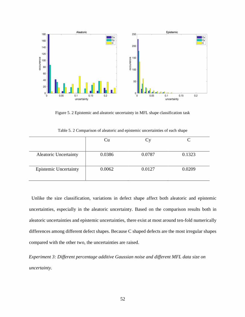
52
Figure 5. 2 Epistemic and aleatoric uncertainty in MFL shape classification task
Table 5. 2 Comparison of aleatoric and epistemic uncertainties of each shape
Cu Cy C
Aleatoric Uncertainty 0.0386 0.0787 0.1323
Epistemic Uncertainty 0.0062 0.0127 0.0209
Unlike the size classification, variations in defect shape affect both aleatoric and epistemic
uncertainties, especially in the aleatoric uncertainty. Based on the comparison results both in
aleatoric uncertainties and epistemic uncertainties, there exist at most around ten-fold numerically
differences among different defect shapes. Because C shaped defects are the most irregular shapes
compared with the other two, the uncertainties are raised.
Experiment 3: Different percentage additive Gaussian noise and different MFL data size on
uncertainty.

53
Here, 0%, 1%, 5% and 10% Gaussian Noise is added to the whole MFL dataset and applied in
the shape and size classification task. In order to clearly and intuitively reflect the noise impacts
on uncertainties, the classification results under one label are chosen to estimate uncertainties,
which are the cubical shaped defect, defects of length 5mm, defects of width 5mm, and defects of
depth 5mm.
Figure 5. 3 Aleatoric and Epistemic uncertainty are computed on the MFL signal with different percentage
noise

54
Figure 5. 3 (cont’d)
It can be seen from the Fig 5.3, no matter in which classification task, noise in data brings much
more uncertainties to the aleatoric part than that to the epistemic part: with the noise inferences,
the average values of aleatoric uncertainties are almost twice larger than previous average values.
In general, the more noises added to MFL data, the larger the aleatoric uncertainty is, but the
epistemic uncertainty is barely changed. This result is consistent with the theory that aleatoric
uncertainty captures the data inherent variation.

55
Besides, different sized MFL data sets are tested in the proposed CNN and Fig 5.4 shows the
corresponding uncertainty results. Original MFL data consists of 243 groups of MFL signals which
is the marked as Data 1. Data 2 is generated by increasing the amount of original MFL data to 324
groups of MFL signal while Data 3 are of 405 groups. Notably, the added MFL data are the
previous MFL data with location alteration. To some extent, the increasing sized data brings
variation (noise) to data as well.

56
Figure 5. 4 Aleatoric, epistemic uncertainty and average uncertainties are computed on each shaped defect
under different data size
From the uncertainty distributions and the trends in average uncertainty values of each shaped
defect in Fig 5.4, it can be seen that with the increased data size, the aleatoric and epistemic
uncertainties are barely changed. Because, in this case, the size of the dataset is not greatly
increased, it is difficult to directly explore the relationship between epistemic uncertainty and the

57
CNN model. However, it has been proved that the aleatoric uncertainty is related with data and in
this experiment the aleatoric uncertainty does not change greatly, therefore, these increased MFL
data don’t bring much data variances. Combined with previous performances that epistemic
uncertainties are barely affected by data intrinsic randomness, in turn, epistemic uncertainty
accounts for the model variation.
58
CONCLUSIONS
To address the problem of defect feature identification in MFL, this thesis work proposed a
novel method based on CNN. Although characteristics of general CNN make it well suited to deal
with images and objects recognition and classification problems, the proposed CNN is applied to
extract defect features directly from the simulated MFL signals and to classify the size and shape
of defects. Further, in the MFL inspection, either the uncertainty in data or model affect prediction
capabilities. Therefore, in order to assess the reliability of the classification results, a Bayesian
inference method is involved in the proposed Convolutional Neural Network to describe the
aleatoric and epistemic uncertainties in physical and machine learning model on defect
identification in MFL inspection. The following conclusions are obtained:
1. Although CNNs are most commonly applied in visual imagery, the proposed CNN provided
good performances in recognizing defect shape and size directly from 3-D MFL signals.
Besides, the proposed CNN has good robustness in position variance and noise distortions on
MFL inspection, especially compared with the traditional machine learning approaches.
2. The comparable performances of the proposed method with previous work in three different
NDT datasets show that the proposed CNN shows great versatility in defect detection in NDE
related areas.
3. The proposed CNN is then combined with a Bayesian inference method to analyze the final
classification results and make the uncertainty estimation to the physical model as well as the
applied classification model on defect identification in MFL inspection.
4. The intrinsic variances in data are proven to be related to the aleatoric uncertainty while the
model variations are described through epistemic uncertainty. In size classification tasks, the

59
different size brings identical uncertainties. Besides, the classification accuracy of the proposed
CNN model is addressed to be negative correlated with the aleatoric uncertainty.

60
FUTURE WORK
To address the problem of defect feature identification in MFL, this thesis work proposed a
novel method based on CNN. According to previous work, the CNN model is a useful tool to
detect and characterize defects in MFL inspection. However, in practical applications, the
defect shape and size vary and normally, there is more than one defect in a measurement area,
therefore, it is necessary to increase the defect variety to explore CNN’s performances on this
problem. Besides, in industry, there are large amounts of MFL signals collected in the pipeline
inspection, and CNNs are good at processing ‘big’ data, it is promising to apply CNN in
classifying practical MFL data.
In addition, the uncertainty estimation approach applied in this thesis only focus on the data
and model. As mentioned before, there exist different kinds of uncertainties in the physical
model, it is necessary to clarify how these uncertainties affect the produced data. If successful,
a reliable MFL defect detection and characterization system could be established and could be
further applied in other NDT techniques, such as ECT.

61
BIBLIOGRAPHY

62
BIBLIOGRAPHY
1. Cartz, L., Nondestructive testing. 1995.
2. Okolo, C. Modelling and experimental investigation of magnetic flux leakage
distribution for hairline crack detection and characterization. Cardiff University,
2018.
3. Rao, B., Magnetic flux leakage technique: basics. J Non Destr Test Eval 2012,
11 (3), 7-17.
4. Okolo, C. K.; Meydan, T., Pulsed magnetic flux leakage method for hairline
crack detection and characterization. AIP Advances 2018, 8 (4), 047207.
5. Zeng, Z.; Udpa, L.; Udpa, S. S.; Chan, M. S. C., Reduced magnetic vector
potential formulation in the finite element analysis of eddy current nondestructive
testing. IEEE transactions on magnetics 2009, 45 (3), 964-967.
6. Piao, G.; Guo, J.; Hu, T.; Deng, Y.; Leung, H., A novel pulsed eddy current
method for high-speed pipeline inline inspection. Sensors and Actuators A: Physical
2019.
7. Snarskii, A.; Zhenirovskyy, M.; Meinert, D.; Schulte, M., An integral
equation model for the magnetic flux leakage method. NDT & E International 2010,
43 (4), 343-347.
8. Wang, Y.; Liu, X.; Wu, B.; Xiao, J.; Wu, D.; He, C., Dipole modeling of
stress-dependent magnetic flux leakage. NDT & E International 2018, 95, 1-8.
9. Zuoying, H.; Peiwen, Q.; Liang, C., 3D FEM analysis in magnetic flux
leakage method. Ndt & E International 2006, 39 (1), 61-66.
10. Alobaidi, W. M.; Alkuam, E. A.; Al-Rizzo, H. M.; Sandgren, E.,
Applications of ultrasonic techniques in oil and gas pipeline industries: a review.
American Journal of Operations Research 2015, 5 (04), 274.
11. Nestleroth, J. B.; Davis, R. J., Application of eddy currents induced by
permanent magnets for pipeline inspection. NDT & E International 2007, 40 (1), 77-
84.

63
12. Xi, G.; Tan, F.; Yan, L.; Huang, C.; Shang, T., Design of an oil pipeline
nondestructive examination system based on ultrasonic testing and magnetic flux
leakage. Revista de la Facultad de Ingeniería 2016, 31 (5), 132-140.
13. Buonsanti, M.; Cacciola, M.; Calcagno, S.; Morabito, F.; Versaci, M. In
Ultrasonic pulse-echoes and eddy current testing for detection, recognition and
characterisation of flaws detected in metallic plates, Proceedings of the 9th European
Conference on Non-Destructive Testing, Citeseer: 2006.
14. Joshi, A.; Udpa, L.; Udpa, S.; Tamburrino, A., Adaptive wavelets for
characterizing magnetic flux leakage signals from pipeline inspection. IEEE
transactions on magnetics 2006, 42 (10), 3168-3170.
15. Shi, Y.; Zhang, C.; Li, R.; Cai, M.; Jia, G., Theory and application of
magnetic flux leakage pipeline detection. Sensors 2015, 15 (12), 31036-31055.
16. Mukhopadhyay, S.; Srivastava, G., Characterisation of metal loss defects
from magnetic flux leakage signals with discrete wavelet transform. Ndt & E
International 2000, 33 (1), 57-65.
17. Mukherjee, D.; Saha, S.; Mukhopadhyay, S., Inverse mapping of magnetic
flux leakage signal for defect characterization. NDT & E International 2013, 54,
198-208.
18. Chen, Z.; Yusa, N.; Miya, K., Some advances in numerical analysis
techniques for quantitative electromagnetic nondestructive evaluation.
Nondestructive testing and evaluation 2009, 24 (1-2), 69-102.
19. Ravan, M.; Amineh, R. K.; Koziel, S.; Nikolova, N. K.; Reilly, J. P., Sizing
of 3-D arbitrary defects using magnetic flux leakage measurements. IEEE
transactions on magnetics 2009, 46 (4), 1024-1033.
20. Chen, Y.; Jiang, H.; Li, C.; Jia, X.; Ghamisi, P., Deep feature extraction and
classification of hyperspectral images based on convolutional neural networks. IEEE
Transactions on Geoscience and Remote Sensing 2016, 54 (10), 6232-6251.
21. He, K.; Zhang, X.; Ren, S.; Sun, J., Spatial pyramid pooling in deep
convolutional networks for visual recognition. IEEE transactions on pattern analysis
and machine intelligence 2015, 37 (9), 1904-1916.

64
22. Feng, J.; Li, F.; Lu, S.; Liu, J.; Ma, D., Injurious or noninjurious defect
identification from MFL images in pipeline inspection using convolutional neural
network. IEEE Transactions on Instrumentation and Measurement 2017, 66 (7),
1883-1892.
23. Der Kiureghian, A.; Ditlevsen, O., Aleatory or epistemic? Does it matter?
Structural Safety 2009, 31 (2), 105-112.
24. Hansen, E., Measure Theory. 4th ed.; 2006.
25. Pijush K. Kundu, I. M. C., David R. Dowling, Fluid Mechanics. Elsevier Inc:
2012.
26. Cook, R. D., Concepts and applications of finite element analysis. John Wiley
& Sons: 2007.
27. Bishop, C. M., Pattern recognition and machine learning. springer: 2006.
28. Segura, J., Orthogonal Polynomials: Computation and Approximation.
JSTOR: 2006.
29. Jäggi, S. B.; Elsener, B., Macrocell Corrosion of Steel in Concrete:
Experiments and numerical modelling. In Corrosion of reinforcement in concrete:
mechanisms, monitoring, inhibitors and rehabilitation techniques, CRC Press: 2007;
Vol. 38, pp 75-104.
30. Zhang, Y.; Ye, Z.; Wang, C., A fast method for rectangular crack sizes
reconstruction in magnetic flux leakage testing. Ndt & E International 2009, 42 (5),
369-375.
31. Keshwani, R. T., Analysis of magnetic flux leakage signals of instrumented
pipeline inspection gauge using finite element method. IETE Journal of Research
2009, 55 (2), 73-82.
32. Pechenkov, A.; Shcherbinin, V.; Smorodinskiy, J., Analytical model of a pipe
magnetization by two parallel linear currents. Ndt & E International 2011, 44 (8),
718-720.
33. Silvester, P. P.; Ferrari, R. L., Finite elements for electrical engineers.
Cambridge university press: 1996.

65
34. Zhou, P.-b., Numerical analysis of electromagnetic fields. Springer Science &
Business Media: 2012.
35. Lord, W.; Udpa, L., Imaging of electromagnetic NDT phenomena. 1986.
36. Schifini, R.; Bruno, A., Experimental verification of a finite element model
used in a magnetic flux leakage inverse problem. Journal of Physics D: Applied
Physics 2005, 38 (12), 1875.
37. Chen, Z.; Preda, G.; Mihalache, O.; Miya, K., Reconstruction of crack shapes
from the MFLT signals by using a rapid forward solver and an optimization
approach. IEEE transactions on magnetics 2002, 38 (2), 1025-1028.
38. Mandache, C.; Clapham, L., A model for magnetic flux leakage signal
predictions. Journal of Physics D: Applied Physics 2003, 36 (20), 2427.
39. Ramuhalli, P.; Udpa, L.; Udpa, S. S., Electromagnetic NDE signal inversion
by function-approximation neural networks. IEEE transactions on magnetics 2002,
38 (6), 3633-3642.
40. Xu, C.; Wang, C.; Ji, F.; Yuan, X., Finite-element neural network-based
solving 3-D differential equations in MFL. IEEE Transactions on Magnetics 2012,
48 (12), 4747-4756.
41. Echeverrĭa, D.; Hemker, P. W., Space mapping and defect correction.
Computational Methods in Applied Mathematics Comput. Methods Appl. Math.
2005, 5 (2), 107-136.
42. Amineh, R. K.; Koziel, S.; Nikolova, N. K.; Bandler, J. W.; Reilly, J. P., A
space mapping methodology for defect characterization from magnetic flux leakage
measurements. IEEE Transactions on Magnetics 2008, 44 (8), 2058-2065.
43. Hoole, S. R. H., Artificial neural networks in the solution of inverse
electromagnetic field problems. IEEE transactions on Magnetics 1993, 29 (2), 1931-
1934.
44. Ramuhalli, P.; Udpa, L.; Udpa, S., Neural network algorithm for
electromagnetic NDE signal inversion. In Electromagnetic Nondestructive
Evaluation (V), IOS: 2001; pp 121-128.

66
45. Joshi, A., Wavelet transform and neural network based 3D defect
characterization using magnetic flux leakage. International Journal of Applied
Electromagnetics and Mechanics 2008, 28 (1-2), 149-153.
46. Priewald, R. H.; Magele, C.; Ledger, P. D.; Pearson, N. R.; Mason, J. S.,
Fast magnetic flux leakage signal inversion for the reconstruction of arbitrary defect
profiles in steel using finite elements. IEEE Transactions on Magnetics 2012, 49 (1),
506-516.
47. Hari, K.; Nabi, M.; Kulkarni, S., Improved FEM model for defect-shape
construction from MFL signal by using genetic algorithm. IET science,
measurement & technology 2007, 1 (4), 196-200.
48. Lijian, Y.; Gang, L.; Guoguang, Z.; Songwei, G. In Oil-gas pipeline magnetic
flux leakage testing defect reconstruction based on support vector machine, 2009
Second International Conference on Intelligent Computation Technology and
Automation, IEEE: 2009; pp 395-398.
49. Mitchell, T., Machine Learning’. McGraw-Hill, New York. NY: 1997.
50. Olden, J. D.; Lawler, J. J.; Poff, N. L., Machine learning methods without
tears: a primer for ecologists. The Quarterly review of biology 2008, 83 (2), 171-
193.
51. Phillips, S. J.; Anderson, R. P.; Schapire, R. E., Maximum entropy modeling
of species geographic distributions. Ecological modelling 2006, 190 (3-4), 231-259.
52. De'ath, G.; Fabricius, K. E., Classification and regression trees: a powerful
yet simple technique for ecological data analysis. Ecology 2000, 81 (11), 3178-3192.
53. Drake, J. M.; Randin, C.; Guisan, A., Modelling ecological niches with
support vector machines. Journal of applied ecology 2006, 43 (3), 424-432.
54. Cho, E.; Chon, T.-S., Application of wavelet analysis to ecological data.
Ecological Informatics 2006, 1 (3), 229-233.
55. Bação, F.; Lobo, V.; Painho, M. In Self-organizing maps as substitutes for k-
means clustering, International Conference on Computational Science, Springer:
2005; pp 476-483.

67
56. Hopfield, J. J., Neural networks and physical systems with emergent
collective computational abilities. Proceedings of the national academy of sciences
1982, 79 (8), 2554-2558.
57. Grounds, M.; Kudenko, D., Parallel reinforcement learning with linear
function approximation. In Adaptive Agents and Multi-Agent Systems III.
Adaptation and Multi-Agent Learning, Springer: 2005; pp 60-74.
58. Tsitsiklis, J. N., Asynchronous stochastic approximation and Q-learning.
Machine learning 1994, 16 (3), 185-202.
59. Mousavi, S. S.; Schukat, M.; Howley, E. In Deep reinforcement learning: an
overview, Proceedings of SAI Intelligent Systems Conference, Springer: 2016; pp
426-440.
60. CireşAn, D.; Meier, U.; Masci, J.; Schmidhuber, J., Multi-column deep
neural network for traffic sign classification. Neural networks 2012, 32, 333-338.
61. Schmidt, U.; Roth, S. In Shrinkage fields for effective image restoration,
Proceedings of the IEEE Conference on Computer Vision and Pattern Recognition,
2014; pp 2774-2781.
62. Graves, A.; Eck, D.; Beringer, N.; Schmidhuber, J. In Biologically plausible
speech recognition with LSTM neural nets, International Workshop on Biologically
Inspired Approaches to Advanced Information Technology, Springer: 2004; pp 127-
136.
63. Gers, F. A.; Schmidhuber, E., LSTM recurrent networks learn simple context-
free and context-sensitive languages. IEEE Transactions on Neural Networks 2001,
12 (6), 1333-1340.
64. Tkachenko, Y., Autonomous CRM control via CLV approximation with deep
reinforcement learning in discrete and continuous action space. arXiv preprint
arXiv:1504.01840 2015.
65. Schmidhuber, J., Deep learning in neural networks: An overview. Neural
networks 2015, 61, 85-117.
66. Zupan, J.; Gasteiger, J., Neural networks for chemists: an introduction. John
Wiley & Sons, Inc.: 1993.

68
67. Khotanzad, A.; Chung, C., Application of multi-layer perceptron neural
networks to vision problems. Neural Computing & Applications 1998, 7 (3), 249-
259.
68. Graves, A.; Schmidhuber, J., Framewise phoneme classification with
bidirectional LSTM and other neural network architectures. Neural networks 2005,
18 (5-6), 602-610.
69. Schmidhuber, J.; Wierstra, D.; Gomez, F. J. In Evolino: Hybrid
neuroevolution/optimal linear search for sequence prediction, Proceedings of the
19th International Joint Conferenceon Artificial Intelligence (IJCAI), 2005.
70. Anumanchipalli, G. K.; Chartier, J.; Chang, E. F., Speech synthesis from
neural decoding of spoken sentences. Nature 2019, 568 (7753), 493.
71. Lawrence, S.; Giles, C. L.; Tsoi, A. C.; Back, A. D., Face recognition: A
convolutional neural-network approach. IEEE transactions on neural networks 1997,
8 (1), 98-113.
72. Ren, S.; He, K.; Girshick, R.; Sun, J. In Faster r-cnn: Towards real-time
object detection with region proposal networks, Advances in neural information
processing systems, 2015; pp 91-99.
73. Siam, M.; Elkerdawy, S.; Jagersand, M.; Yogamani, S. In Deep semantic
segmentation for automated driving: Taxonomy, roadmap and challenges, 2017
IEEE 20th International Conference on Intelligent Transportation Systems (ITSC),
IEEE: 2017; pp 1-8.
74. Ito, Y., Representation of functions by superpositions of a step or sigmoid
function and their applications to neural network theory. Neural Networks 1991, 4
(3), 385-394.
75. Maas, A. L.; Hannun, A. Y.; Ng, A. Y. In Rectifier nonlinearities improve
neural network acoustic models, Proc. icml, 2013; p 3.
76. Glorot, X.; Bordes, A.; Bengio, Y. In Deep sparse rectifier neural networks,
Proceedings of the fourteenth international conference on artificial intelligence and
statistics, 2011; pp 315-323.

69
77. Ramachandran, P.; Zoph, B.; Le, Q. V., Searching for activation functions.
arXiv preprint arXiv:1710.05941 2017.
78. Nam, H.; Han, B. In Learning multi-domain convolutional neural networks
for visual tracking, Proceedings of the IEEE conference on computer vision and
pattern recognition, 2016; pp 4293-4302.
79. Havaei, M.; Davy, A.; Warde-Farley, D.; Biard, A.; Courville, A.; Bengio,
Y.; Pal, C.; Jodoin, P.-M.; Larochelle, H., Brain tumor segmentation with deep
neural networks. Medical image analysis 2017, 35, 18-31.
80. Zhu, P.; Cheng, Y.; Banerjee, P.; Tamburrino, A.; Deng, Y., A novel
machine learning model for eddy current testing with uncertainty. NDT & E
International 2019, 101, 104-112.
81. Li, F.; Feng, J.; Lu, S.; Liu, J.; Yao, Y. In Convolution neural network for
classification of magnetic flux leakage response segments, 2017 6th Data Driven
Control and Learning Systems (DDCLS), IEEE: 2017; pp 152-155.
82. Urbina, A., Uncertainty quantification and decision making in hierarchical
development of computational models. 2009; Vol. 73.
83. Ma, Y.; Wang, L.; Zhang, J.; Xiang, Y.; Peng, T.; Liu, Y., Hybrid
uncertainty quantification for probabilistic corrosion damage prediction for aging
RC bridges. Journal of Materials in Civil Engineering 2014, 27 (4), 04014152.
84. Hemez, F. M.; Roberson, A.; Rutherford, A. C. In Uncertainty quantification
and model validation for damage prognosis, the Proceedings of the 4th International
Workshop on Structural Health Monitoring, Stanford University, Stanford,
California, 2003.
85. Alberts, E.; Rempfler, M.; Alber, G.; Huber, T.; Kirschke, J.; Zimmer, C.;
Menze, B. H. In Uncertainty quantification in brain tumor segmentation using CRFs
and random perturbation models, 2016 IEEE 13th International Symposium on
Biomedical Imaging (ISBI), IEEE: 2016; pp 428-431.
86. Neal, R. M. In Bayesian learning via stochastic dynamics, Advances in neural
information processing systems, 1993; pp 475-482.

70
87. Graves, A. In Practical variational inference for neural networks, Advances in
neural information processing systems, 2011; pp 2348-2356.
88. Blundell, C.; Cornebise, J.; Kavukcuoglu, K.; Wierstra, D., Weight
uncertainty in neural networks. arXiv preprint arXiv:1505.05424 2015.
89. Fortunato, M.; Blundell, C.; Vinyals, O., Bayesian recurrent neural networks.
arXiv preprint arXiv:1704.02798 2017.
90. Shridhar, K.; Laumann, F.; Liwicki, M., A comprehensive guide to bayesian
convolutional neural network with variational inference. arXiv preprint
arXiv:1901.02731 2019.
91. Neklyudov, K.; Molchanov, D.; Ashukha, A.; Vetrov, D., Variance networks:
When expectation does not meet your expectations. arXiv preprint
arXiv:1803.03764 2018.
92. Srivastava, N.; Hinton, G.; Krizhevsky, A.; Sutskever, I.; Salakhutdinov, R.,
Dropout: a simple way to prevent neural networks from overfitting. The journal of
machine learning research 2014, 15 (1), 1929-1958.
93. Wang, S.; Manning, C. In Fast dropout training, international conference on
machine learning, 2013; pp 118-126.
94. Kingma, D. P.; Salimans, T.; Welling, M. In Variational dropout and the local
reparameterization trick, Advances in Neural Information Processing Systems, 2015;
pp 2575-2583.
95. Gal, Y.; Ghahramani, Z., Bayesian convolutional neural networks with
Bernoulli approximate variational inference. arXiv preprint arXiv:1506.02158 2015.
96. Gal, Y.; Ghahramani, Z. In Dropout as a Bayesian approximation: Insights
and applications, Deep Learning Workshop, ICML, 2015; p 2.
97. Kendall, A.; Gal, Y. In What uncertainties do we need in bayesian deep
learning for computer vision?, Advances in neural information processing systems,
2017; pp 5574-5584.
98. Feng, J.; Lu, S.; Liu, J.; Li, F., A sensor liftoff modification method of
magnetic flux leakage signal for defect profile estimation. IEEE Transactions on
Magnetics 2017, 53 (7), 1-13.

71
99. Lu, S.; Feng, J.; Li, F.; Liu, J.; Zhang, H. In Extracting defect signal from
the MFL signal of seamless pipeline, 2017 29th Chinese Control And Decision
Conference (CCDC), IEEE: 2017; pp 5209-5212.
100. Afzal, M.; Polikar, R.; Udpa, L.; Udpa, S. In Adaptive noise cancellation
schemes for magnetic flux leakage signals obtained from gas pipeline inspection,
2001 IEEE International Conference on Acoustics, Speech, and Signal Processing.
Proceedings (Cat. No. 01CH37221), IEEE: 2001; pp 3389-3392.
101. Chen, L.; Li, X.; Qin, G.; Lu, Q., Signal processing of magnetic flux leakage
surface flaw inspect in pipeline steel. Russian Journal of Nondestructive Testing
2008, 44 (12), 859-867.
102. Ji, F.; Wang, C.; Sun, S.; Wang, W., Application of 3-D FEM in the
simulation analysis for MFL signals. Insight-Non-Destructive Testing and Condition
Monitoring 2009, 51 (1), 32-35.
103. Langton, C.; Pisharody, S.; Keyak, J., Comparison of 3D finite element
analysis derived stiffness and BMD to determine the failure load of the excised
proximal femur. Medical engineering & physics 2009, 31 (6), 668-672.
104. Lewis, R.; Huang, H.; Usmani, A.; Cross, J., Finite element analysis of heat
transfer and flow problems using adaptive remeshing including application to
solidification problems. International journal for numerical methods in engineering
1991, 32 (4), 767-781.
105. Ansari, S.; Farquharson, C. G., 3D finite-element forward modeling of
electromagnetic data using vector and scalar potentials and unstructured grids.
Geophysics 2014, 79 (4), E149-E165.
106. Martin, H. C.; Carey, G. F., Introduction to finite element analysis: theory and
application. McGraw-Hill College: 1973.
107. Yang, S., Finite element modeling of current perturbation method of
nondestructive evaluation application. 2000.
108. Jianming, J., The Finite Element Method of the Electromagnetic [M]. Xidian
University Press: Xi’an, 1998; p
.

72
109. Gupta, A.; Chandrasekaran, K., Finite element modeling of magnetic flux
leakage from metal loss defects in steel pipeline. Journal of Failure Analysis and
Prevention 2016, 16 (2), 316-323.
110. Wolfe, J.; Jin, X.; Bahr, T.; Holzer, N., Application of softmax regression
and its validation for spectral-based land cover mapping. The International Archives
of Photogrammetry, Remote Sensing and Spatial Information Sciences 2017, 42,
455.
111. Martins, A.; Astudillo, R. In From softmax to sparsemax: A sparse model of
attention and multi-label classification, International Conference on Machine
Learning, 2016; pp 1614-1623.
112. Zhang, L.; Yang, F.; Zhang, Y. D.; Zhu, Y. J. In Road crack detection using
deep convolutional neural network, 2016 IEEE international conference on image
processing (ICIP), IEEE: 2016; pp 3708-3712.
113. Özgenel, Ç. F., Concrete Crack Images for Classification. 2018.
114. Li, W.-b.; Lu, C.-h.; Zhang, J.-c., A lower envelope Weber contrast detection
algorithm for steel bar surface pit defects. Optics & Laser Technology 2013, 45,
654-659.
115. Martin, D.; Guinea, D. M.; García-Alegre, M. C.; Villanueva, E.; Guinea,
D., Multi-modal defect detection of residual oxide scale on a cold stainless steel strip.
Machine Vision and Applications 2010, 21 (5), 653-666.
116. Song, K.; Hu, S.; Yan, Y., Automatic recognition of surface defects on hot-
rolled steel strip using scattering convolution network. Journal of Computational
Information Systems 2014, 10 (7), 3049-3055.
117. Ren, R.; Hung, T.; Tan, K. C., A generic deep-learning-based approach for
automated surface inspection. IEEE transactions on cybernetics 2017, 48 (3), 929-
940.
118. He, Y.; Song, K.; Meng, Q.; Yan, Y., An End-to-end Steel Surface Defect
Detection Approach via Fusing Multiple Hierarchical Features. IEEE Transactions
on Instrumentation and Measurement 2019.

73
119. Donahue, J.; Jia, Y.; Vinyals, O.; Hoffman, J.; Zhang, N.; Tzeng, E.; Darrell,
T. In Decaf: A deep convolutional activation feature for generic visual recognition,
International conference on machine learning, 2014; pp 647-655.
120. Cimpoi, M.; Maji, S.; Kokkinos, I.; Mohamed, S.; Vedaldi, A. In Describing
textures in the wild, Proceedings of the IEEE Conference on Computer Vision and
Pattern Recognition, 2014; pp 3606-3613.
121. Yosinski, J.; Clune, J.; Bengio, Y.; Lipson, H. In How transferable are
features in deep neural networks?, Advances in neural information processing
systems, 2014; pp 3320-3328.
122. Sharif Razavian, A.; Azizpour, H.; Sullivan, J.; Carlsson, S. In CNN features
off-the-shelf: an astounding baseline for recognition, Proceedings of the IEEE
conference on computer vision and pattern recognition workshops, 2014; pp 806-
813.
123. Virkkunen, I.; Koskinen, T.; Jessen-Juhler, O.; Rinta-Aho, J., Augmented
Ultrasonic Data for Machine Learning. arXiv preprint arXiv:1903.11399 2019.
124. Pal, M.; Mather, P. M., An assessment of the effectiveness of decision tree
methods for land cover classification. Remote sensing of environment 2003, 86 (4),
554-565.
125. Srivastava, A.; Han, E.-H.; Kumar, V.; Singh, V., Parallel formulations of
decision-tree classification algorithms. In High Performance Data Mining, Springer:
1999; pp 237-261.
126. Mathur, A.; Foody, G. M., Multiclass and binary SVM classification:
Implications for training and classification users. IEEE Geoscience and remote
sensing letters 2008, 5 (2), 241-245.
127. Foody, G. M.; Mathur, A., Toward intelligent training of supervised image
classifications: directing training data acquisition for SVM classification. Remote
Sensing of Environment 2004, 93 (1-2), 107-117.
128. Moreno, P. J.; Ho, P. P.; Vasconcelos, N. In A Kullback-Leibler divergence
based kernel for SVM classification in multimedia applications, Advances in neural
information processing systems, 2004; pp 1385-1392.

74
129. Bazi, Y.; Melgani, F., Toward an optimal SVM classification system for
hyperspectral remote sensing images. IEEE Transactions on geoscience and remote
sensing 2006, 44 (11), 3374-3385.
130. Ye, P. In The decision tree classification and its application research in
personnel management, Proceedings of 2011 International Conference on
Electronics and Optoelectronics, IEEE: 2011; pp V1-372-V1-375.
131. Nazari, Z.; Kang, D., Density based support vector machines for classification.
International Journal of Advacnced Research in Artificial Intelligence (IJARAI)
2015, 4 (4).
132. Kecman, V., Learning and soft computing: support vector machines, neural
networks, and fuzzy logic models. MIT press: 2001.
133. Abe, S., Support vector machines for pattern classification. Springer: 2005;
Vol. 2.
134. Vapnik, V.; Vapnik, V., Statistical learning theory Wiley. New York 1998,
156-160.
135. Piao, G.; Guo, J.; Hu, T.; Leung, H.; Deng, Y., Fast reconstruction of 3-D
defect profile from MFL signals using key physics-based parameters and SVM.
NDT & E International 2019, 103, 26-38.
136. Pradhan, S. S.; Ward, W. H.; Hacioglu, K.; Martin, J. H.; Jurafsky, D. In
Shallow semantic parsing using support vector machines, Proceedings of the Human
Language Technology Conference of the North American Chapter of the
Association for Computational Linguistics: HLT-NAACL 2004, 2004; pp 233-240.
137. Barghout, L., Spatial-taxon information granules as used in iterative fuzzy-
decision-making for image segmentation. In Granular Computing and Decision-
Making, Springer: 2015; pp 285-318.
138. Statnikov, A.; Hardin, D.; Aliferis, C., Using SVM weight-based methods to
identify causally relevant and non-causally relevant variables. sign 2006, 1 (4).
139. Sharma, P.; Kaur, M., Classification in pattern recognition: A review.
International Journal of Advanced Research in Computer Science and Software
Engineering 2013, 3 (4).

75
140. Kamavisdar, P.; Saluja, S.; Agrawal, S., A survey on image classification
approaches and techniques. International Journal of Advanced Research in
Computer and Communication Engineering 2013, 2 (1), 1005-1009.
141. D'Angelo, G.; Rampone, S. In Shape-based defect classification for non
destructive testing, 2015 IEEE Metrology for Aerospace (MetroAeroSpace), IEEE:
2015; pp 406-410.
142. Kwon, Y.; Won, J.-H.; Kim, B. J.; Paik, M. C., Uncertainty quantification
using bayesian neural networks in classification: Application to ischemic stroke
lesion segmentation. 2018.