Deep Learning in Microsoft with CNTK

Alexey Kamenev

Microsoft Research

S6843

Deep Learning in the company

•Bing • Cortana

• Ads

• Relevance

• Multimedia

• …

•Skype

•HoloLens

•Research • Speech, image, text

2

2015 System

Human Error Rate 4%

ImageNet: Microsoft 2015 ResNet

28.2 25.8

16.4

11.7

7.3 6.7 3.5

ILSVRC2010 NECAmerica

ILSVRC2011 Xerox

ILSVRC2012

AlexNet

ILSVRC2013 Clarifi

ILSVRC2014 VGG

ILSVRC2014

GoogleNet

ILSVRC2015 ResNet

ImageNet Classification top-5 error (%)

Microsoft had all 5 entries being the 1-st places this year: ImageNet classification,

ImageNet localization, ImageNet detection, COCO detection, and COCO segmentation

CNTK Overview •A deep learning tool that balances

• Efficiency: Can train production systems as fast as possible • Performance: Can achieve state-of-the-art performance on

benchmark tasks and production systems • Flexibility: Can support various tasks such as speech, image, and

text, and can try out new ideas quickly

• Inspiration: Legos • Each brick is very simple and performs a specific function • Create arbitrary objects by combining many bricks

•CNTK enables the creation of existing and novel models by combining simple functions in arbitrary ways. •Historical facts:

• Created by Microsoft Speech researchers (Dong Yu et al.) 4 years ago • Was quickly extended to handle other workloads (image/text)

• Open-sourced (CodePlex) in early 2015 • Moved to GitHub in Jan 2016

5

Functionality • Supports

• CPU and GPU with a focus on GPU Cluster • GPU (CUDA): uses NVIDIA libraries, including cuDNN v5.

• Windows and Linux • automatic numerical differentiation • efficient static and recurrent network training through batching • data parallelization within and across machines with 1-bit

quantized SGD • memory sharing during execution planning

• Modularized: separation of • computational networks • execution engine • learning algorithms • model description • data readers

• Models can be described and modified with • Network definition language (NDL) and model editing language (MEL) • Python, C++ and C# (in progress)

6

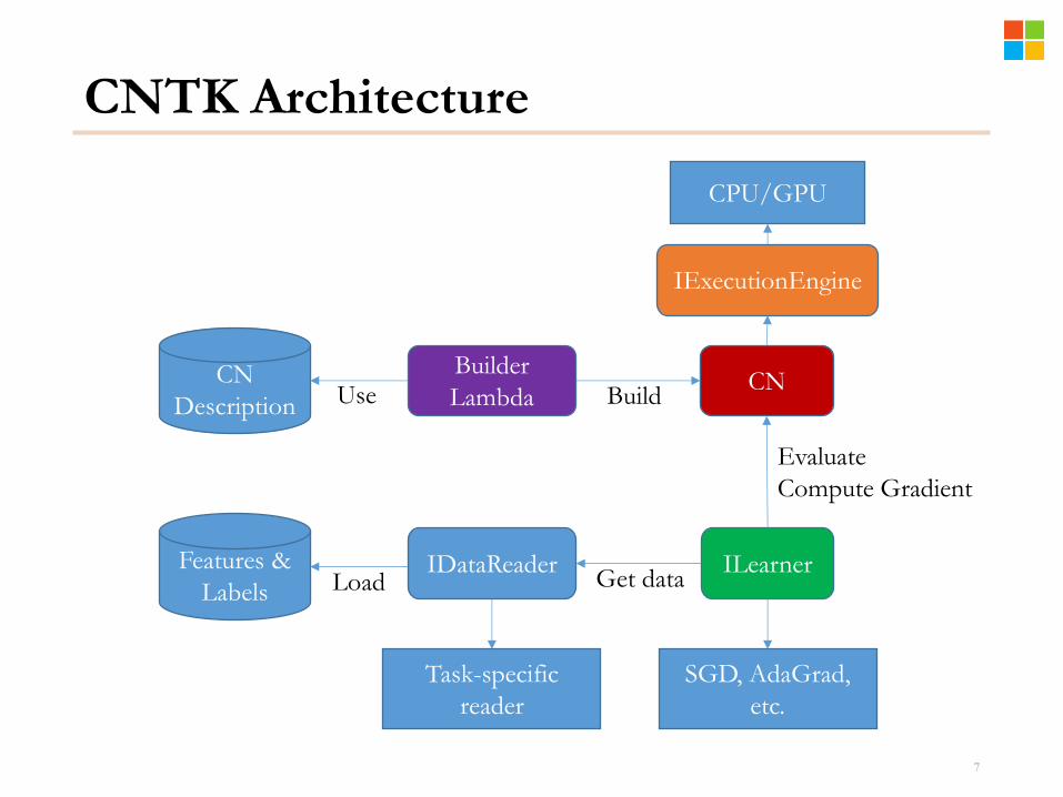
CNTK Architecture

7

CN Builder

Lambda CN

Description Use Build

ILearner IDataReader Features &

Labels Load Get data

IExecutionEngine

CPU/GPU

Task-specific

reader

SGD, AdaGrad,

etc.

Evaluate

Compute Gradient

Main Operations

•Train a model with the train command

•Evaluate a model with the eval command

•Edit models (e.g., add nodes, remove nodes, change the flag of a node) with the edit command

•Write outputs of one or more nodes in the model to files with the write command

•Finer operation can be controlled through script languages (beta)

8

At the Heart: Computational Networks

•A generalization of machine learning models that can be described as a series of computational steps. • E.g., DNN, CNN, RNN, LSTM, DSSM, Log-linear model

•Representation: • A list of computational nodes denoted as n = {node name : operation name} • The parent-children relationship describing the operands {n : c1, · · · , cKn }

• Kn is the number of children of node n. For leaf nodes Kn = 0.

• Order of the children matters: e.g., XY is different from YX

• Given the inputs (operands) the value of the node can be computed.

•Can flexibly describe deep learning models. • Adopted by many other popular tools as well

9

Example: One Hidden Layer NN

10

O

P(1)

X

W(1), b(1)

W(2), b(2)

S(1)

Sigmoid

P(2)

Softmax

Hidden

Layer

Output

Layer

Example: CN with Multiple Inputs

11

Example: CN with Recurrence

12

Usage Example (with Config File) • cntk configFile=yourConfigFile DeviceNumber=1

13

command=Train:Test

Train=[

action = "train"

deviceId=$DeviceNumber$

modelPath=“$your_model_path$

NDLNetworkBuilder=[…]

SGD=[…]

reader=[…]

]

String Replacement

CPU: CPU

GPU: >=0 or auto

• You can also use C++, Python and C# (work in progress) to directly instantiate related objects.

Network Definition with NDL (LSTM)

14

Network Definition with NDL

15

LSTMComponent(inputDim, outputDim, inputVal) = [

Wxo = Parameter(outputDim, inputDim)

Wxi = Parameter(outputDim, inputDim)

Wxf = Parameter(outputDim, inputDim)

Wxc = Parameter(outputDim, inputDim)

bo = Parameter(outputDim, 1, init=fixedvalue, value=-1.0)

bc = Parameter(outputDim, 1, init=fixedvalue, value=0.0)

bi = Parameter(outputDim, 1, init=fixedvalue, value=-1.0)

bf = Parameter(outputDim, 1, init=fixedvalue, value=-1.0)

Whi = Parameter(outputDim, outputDim)

Wci = Parameter(outputDim , 1)

Whf = Parameter(outputDim, outputDim)

Wcf = Parameter(outputDim , 1)

Who = Parameter(outputDim, outputDim)

Wco = Parameter(outputDim , 1)

Whc = Parameter(outputDim, outputDim)

parameters

Wrapped as a macro and

can be reused

Network Definition with NDL

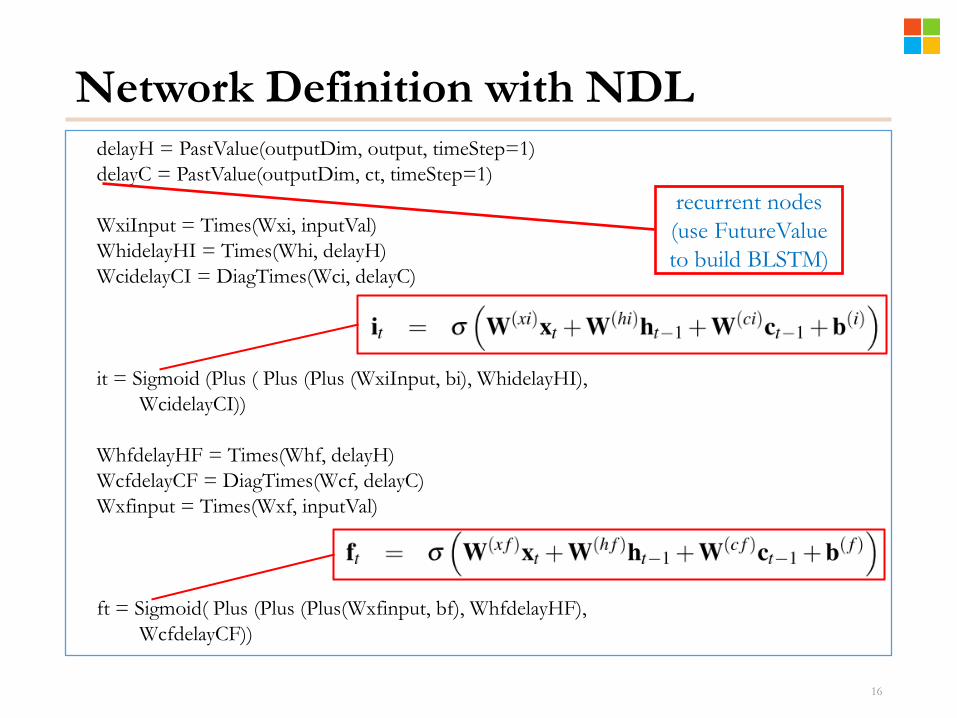
16

delayH = PastValue(outputDim, output, timeStep=1)

delayC = PastValue(outputDim, ct, timeStep=1)

WxiInput = Times(Wxi, inputVal)

WhidelayHI = Times(Whi, delayH)

WcidelayCI = DiagTimes(Wci, delayC)

it = Sigmoid (Plus ( Plus (Plus (WxiInput, bi), WhidelayHI),

WcidelayCI))

WhfdelayHF = Times(Whf, delayH)

WcfdelayCF = DiagTimes(Wcf, delayC)

Wxfinput = Times(Wxf, inputVal)

ft = Sigmoid( Plus (Plus (Plus(Wxfinput, bf), WhfdelayHF),

WcfdelayCF))

recurrent nodes

(use FutureValue

to build BLSTM)

Network Definition with NDL

17

•Convolutions (2D and ND)

•Simple Syntax for 2D convolutions:

ConvReLULayer(inp, outMap, inWCount, kW, kH, hStride, vStride, wScale, bValue)

[ W = LearnableParameter(outMap, inWCount, init = Gaussian, initValueScale = wScale)

b = ImageParameter(1, 1, outMap, init = fixedValue, value = bValue)

c = Convolution(W, inp, kW, kH, outMap, hStride, vStride, zeroPadding = true) p = Plus(c, b)

y = RectifiedLinear(p)

]

# conv2

kW2 = 5

kH2 = 5

map2 = 32

hStride2 = 1

vStride2 = 1 conv2 = ConvReLULayer(pool1, map2, 800, kW2, kH2, hStride2, vStride2, conv2WScale, conv2BValue)

Macro usage

Reusable macro

Network Definition with NDL

18

•Powerful syntax for ND convolutions: Convolution(w, input,

{kernel dimensions},

mapCount = {map dimensions},

stride = {stride dimensions},

sharing = {sharing},

autoPadding = {padding (boolean)},

lowerPad = {lower padding (int)},

upperPad = {upper padding (int)})

ConvLocalReLULayer(inp, outMap, outWCount, inMap, inWCount, kW, kH, hStride, vStride, wScale, bValue)

[

W = LearnableParameter(outWCount, inWCount, init = Gaussian, initValueScale = wScale)

b = ImageParameter(1, 1, outMap, init = fixedValue, value = bValue)

c = Convolution(W, inp,

{kW, kH, inMap},

mapCount = outMap,

stride = {hStride, vStride, inMap},

sharing = {false, false, false})

p = Plus(c, b)

y = RectifiedLinear(p)

]

Sharing is disabled –

enables locally

connected convolutions

Network Definition with NDL

19

•Same engine and syntax for pooling: Pooling(input, poolKind

{kernel dimensions},

stride = {stride dimensions},

autoPadding = {padding (boolean)},

lowerPad = {lower padding (int)},

upperPad = {upper padding (int)})

MaxoutLayer(inp, kW, kH, kC, hStride, vStride, cStride)

[

c = Pooling(inp, “max”,

{kW, kH, kC},

stride = {hStride, vStride, cStride})

]

Pool and stride in any

way you like

Model Editing with MEL

X

CE.S=Softmax(CE.P) CE.P=Plus(CE.T,bO) CE.T=Times(WO,L1.S)

L1.S=Sigmoid(CE.P) L1.P=Plus(L1.T,b1) L1.T=Times(W1,X)

X

L2.S=Sigmoid(L2.P) L2.P=Plus(L2.T,bO) L2.T=Times(W2,L1.S)

L1.S=Sigmoid(CE.P) L1.P=Plus(L1.T,b1) L1.T=Times(W1,X)

CE.S=Softmax(CE.P) CE.P=Plus(CE.T,bO) CE.T=Times(WO*L2.S)

MO

DIF

Y

CR

EA

TE

MEL

20

Insert a new layer (e.g., for

discriminative pretraining)

Computation: Without Loops

•Given the root node, the computation order can be determined by a depth-first traverse of the directed acyclic graph (DAG).

•Only need to run it once and cache the order

•Can easily parallelize on the whole minibatch to speed up computation

21

With Loops (Recurrent Connections)

• Naive solution: • Unroll whole graph over time

• Compute sample by sample

22

Implemented with

Delay (PastValue or

FutureValue) node

Very important in many interesting models

With Loops (Recurrent Connections)

•We developed a smart algorithm to analyze the computational network so that we can • Find loops in arbitrary computational networks

• Do whole minibatch computation on everything except nodes inside loops

• Group multiple sequences with variable lengths (better convergence property than tools that only support batching of same length sequences)

23

[CATEGORY NAME], Single

Sequence, [VALUE]

[CATEGORY NAME], multi

sequence >[VALUE]

0 5 10 15 20 25

Naïve

Optimized

Speed comparison on RNNs

Users just describe

computation steps.

Speed up is automatic

Data Parallelization: 1-Bit Quantized SGD

•Bottleneck for distributed learning: Communication cost

• Solution: reduce the amount of data need to be communicated by quantizing gradients to just 1 bit • It’s a lot safer to quantize gradients than model parameters and

outputs (gradients are small and noisy anyway) • Carry quantization residue to next minibatch (important)

• Further hide communication with double-buffering: send one while processing the other

• Use an O(1) communication scheduler to sync gradients • Increase minibatch size to fully utilize each GPU as early as

possible

24

0 5 10 15 20 25 30 35

1-bit

float

Transferred Gradient (bits/value), smaller is better

1-Bit Stochastic Gradient Descent and its Application to Data-Parallel Distributed Training of Speech DNNs, InterSpeech

2014, F. Seide, H. Fu, J. Droppo, G. Li, D. Yu

O(1) Aggregation

25

1 1 1 2 2 2 3 3 3

1+3 1 1 2 1+2 2 3 3 2+3

1+2+

3 1 1 2

1+2+

3 2 3 3

3+2+

1

CNTK = Cinderella NTK?

26

[CATEGORY NAME] only

supports 1 GPU

Achieved with 1-bit gradient quantization algorithm

0

10000

20000

30000

40000

50000

60000

70000

80000

CNTK Theano TensorFlow Torch 7 Caffe

Speed Comparison (Frames/Second, The Higher the Better)

1 GPU 1 x 4 GPUs 2 x 4 GPUs (8 GPUs)

CNTK Computational Performance

Memory Sharing

•Use same memory across minibatches: don’t destroy and reallocate memory at each minibatch.

•Share memory across computation nodes when possible • Analyze the execution plan and release the memory to a

pool to be reused by other nodes or computation if possible

• E.g., when a node finished computing all its children’s gradients, the matrices owned by that node can all be released.

• Can reduce memory by 1/3 to 1/2 for training in most cases

• Can reduce memory even more if gradients are not needed.

27

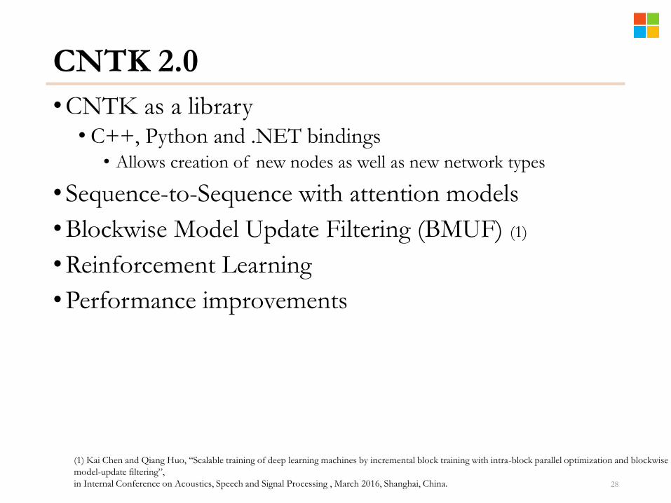
CNTK 2.0

•CNTK as a library • C++, Python and .NET bindings

• Allows creation of new nodes as well as new network types

•Sequence-to-Sequence with attention models

•Blockwise Model Update Filtering (BMUF) (1)

•Reinforcement Learning

•Performance improvements

28

(1) Kai Chen and Qiang Huo, “Scalable training of deep learning machines by incremental block training with intra-block parallel optimization and blockwise

model-update filtering”,

in Internal Conference on Acoustics, Speech and Signal Processing , March 2016, Shanghai, China.

Summary

•CNTK is a powerful tool that supports CPU/GPU and runs under Windows/Linux

•CNTK is extensible with the low-coupling modular design: adding new readers and new computation nodes is easy with a new reader design

•Network definition language, macros, and model editing language (as well as Python and C++ bindings in the future) makes network design and modification easy

•Compared to other tools CNTK has a great balance between efficiency, performance, and flexibility

29

Azure GPU Lab (Project Philly) - Coming

•High performance deep learning platform on Azure

•Scalable to hundreds of NVIDIA GPUs

•Rapid, no-hassle, deep learning experimentation

•Larger models and training data sets

•Multitenant

•Fault tolerant

•Open source friendly

•CNTK optimized

•3rd party accessible (coming)

• The project has been running internally for 6+ months with great success

30

Project Philly Architecture

31

HDFS (Distributed Storage)

YARN (Job/Container Scheduling,

Resource Management)

CoreOS

CNTK

JobA User0

Node0

GPU0,1,2,3

CNTK

JobA User0

Node1

GPU0,1,2,3

Docker (Ubuntu Distribution)

CNTK

JobC User2

Node2

GPU2

… CNTK

JobB User1

Node2

GPU1

Web

Portal

Samba

REST

API

FUSE

Project Philly Job Monitoring

32

Project Philly Cluster Monitoring

33

Additional Resources

•CNTK: • https://github.com/Microsoft/CNTK

• Contains all the source code and example setups

• You may understand better how CNTK works by reading the source code

• New features are added constantly

•How to contact: • CNTK team: ask a question on CNTK GitHub!

• Alexey: • Email: alexey.kamenev@microsoft.com

• : https://www.linkedin.com/in/alexeykamenev

34