deep learning in agriculture: a survey
TRANSCRIPT

1
Deep Learning in Agriculture: A Survey
Andreas Kamilaris1 and Francesc X. Prenafeta-Boldú
Institute for Food and Agricultural Research and Technology (IRTA)
Abstract: Deep learning constitutes a recent, modern technique for image processing and
data analysis, with promising results and large potential. As deep learning has been
successfully applied in various domains, it has recently entered also the domain of
agriculture. In this paper, we perform a survey of 40 research efforts that employ deep
learning techniques, applied to various agricultural and food production challenges. We
examine the particular agricultural problems under study, the specific models and
frameworks employed, the sources, nature and pre-processing of data used, and the
overall performance achieved according to the metrics used at each work under study.
Moreover, we study comparisons of deep learning with other existing popular techniques,
in respect to differences in classification or regression performance. Our findings indicate
that deep learning provides high accuracy, outperforming existing commonly used image
processing techniques.
Keywords: Deep learning, Agriculture, Survey, Convolutional Neural Networks, Recurrent
Neural Networks, Smart Farming, Food Systems.
1 Corresponding Author. Email: [email protected]

2
1. Introduction
Smart farming (Tyagi, 2016) is important for tackling the challenges of agricultural
production in terms of productivity, environmental impact, food security and sustainability
(Gebbers & Adamchuk, 2010). As the global population has been continuously increasing
(Kitzes, et al., 2008), a large increase on food production must be achieved (FAO, 2009),
maintaining at the same time availability and high nutritional quality across the globe,
protecting the natural ecosystems by using sustainable farming procedures.
To address these challenges, the complex, multivariate and unpredictable agricultural
ecosystems need to be better understood by monitoring, measuring and analyzing
continuously various physical aspects and phenomena. This implies analysis of big
agricultural data (Kamilaris, Kartakoullis, & Prenafeta-Boldú, A review on the practice of
big data analysis in agriculture, 2017), and the use of new information and communication
technologies (ICT) (Kamilaris, Gao, Prenafeta-Boldú, & Ali, 2016), both for short-scale
crop/farm management as well as for larger-scale ecosystems’ observation, enhancing the
existing tasks of management and decision/policy making by context, situation and
location awareness. Larger-scale observation is facilitated by remote sensing
(Bastiaanssen, Molden, & Makin, 2000), performed by means of satellites, airplanes and
unmanned aerial vehicles (UAV) (i.e. drones), providing wide-view snapshots of the
agricultural environments. It has several advantages when applied to agriculture, being a
well-known, non-destructive method to collect information about earth features while data
may be obtained systematically over large geographical areas.
A large subset of the volume of data collected through remote sensing involve images.
Images constitute, in many cases, a complete picture of the agricultural environments and
could address a variety of challenges (Liaghat & Balasundram, 2010), (Ozdogan, Yang,
Allez, & Cervantes, 2010). Hence, imaging analysis is an important research area in the
agricultural domain and intelligent data analysis techniques are being used for image
3
identification/classification, anomaly detection etc., in various agricultural applications
(Teke, Deveci, Haliloğlu, Gürbüz, & Sakarya, 2013), (Saxena & Armstrong, 2014), (Singh,
Ganapathysubramanian, Singh, & Sarkar, 2016). The most popular techniques and
applications are presented in Appendix I, together with the sensing methods employed to
acquire the images. From existing sensing methods, the most common one is satellite-
based, using multi-spectral and hyperspectral imaging. Synthetic aperture radar (SAR),
thermal and near infrared (NIR) cameras are being used in a lesser but increasing extent
(Ishimwe, Abutaleb, & Ahmed, 2014), while optical and X-ray imaging are being applied in
fruit and packaged food grading. The most popular techniques used for analyzing images
include machine learning (ML) (K-means, support vector machines (SVM), artificial neural
networks (ANN) amongst others), linear polarizations, wavelet-based filtering, vegetation
indices (NDVI) and regression analysis (Saxena & Armstrong, 2014), (Singh,
Ganapathysubramanian, Singh, & Sarkar, 2016).
Besides the aforementioned techniques, a new one which is recently gaining momentum is
deep learning (DL) (LeCun, Bengio, & Hinton, 2015), (LeCun & Bengio, 1995). DL belongs
to the machine learning computational field and is similar to ANN. However, DL is about
“deeper” neural networks that provide a hierarchical representation of the data by means
of various convolutions. This allows larger learning capabilities and thus higher
performance and precision. A brief description of DL is attempted in Section 3.
The motivation for preparing this survey stems from the fact that DL in agriculture is a
recent, modern and promising technique with growing popularity, while advancements and
applications of DL in other domains indicate its large potential. The fact that today there
exists at least 40 research efforts employing DL to address various agricultural problems
with very good results, encouraged the authors to prepare this survey. To the authors’
knowledge, this is the first such survey in the agricultural domain, while a small number of
more general surveys do exist (Deng & Yu, 2014), (Wan, et al., 2014), (Najafabadi, et al.,

4
2015), covering related work in DL in other domains.
2. Methodology
The bibliographic analysis in the domain under study involved two steps: a) collection of
related work and b) detailed review and analysis of this work. In the first step, a keyword-
based search for conference papers or journal articles was performed from the scientific
databases IEEE Xplore and ScienceDirect, and from the web scientific indexing services
Web of Science and Google Scholar. As search keywords, we used the following query:
["deep learning"] AND ["agriculture" OR ”farming"]
In this way, we filtered out papers referring to DL but not applied to the agricultural domain.
From this effort, 47 papers had been initially identified. Restricting the search for papers
with appropriate application of the DL technique and meaningful findings2, the initial
number of papers reduced to 40.
In the second step, the 40 papers selected from the previous step were analyzed one-by-
one, considering the following research questions:
1. Which was the agricultural- or food-related problem they addressed?
2. Which was the general approach and type of DL-based models employed?
3. Which sources and types of data had been used?
4. Which were the classes and labels as modeled by the authors? Were there any
variations among them, observed by the authors?
5. Any pre-processing of the data or data augmentation techniques used?
6. Which has been the overall performance depending on the metric adopted?
7. Did the authors test the performance of their models on different datasets?
8. Did the authors compare their approach with other techniques and, if yes, which
was the difference in performance?
Our main findings are presented in Section 4 and the detailed information per paper is
2 A small number of papers claimed of using DL in some agricultural-related application, but they did not show any results nor provided performance metrics that could indicate the success of the technique used.
5
listed in Appendix II.
3. Deep Learning
DL extends classical ML by adding more "depth" (complexity) into the model as well as
transforming the data using various functions that allow data representation in a
hierarchical way, through several levels of abstraction (Schmidhuber, 2015), (LeCun &
Bengio, 1995). A strong advantage of DL is feature learning, i.e. the automatic feature
extraction from raw data, with features from higher levels of the hierarchy being formed by
the composition of lower level features (LeCun, Bengio, & Hinton, 2015). DL can solve
more complex problems particularly well and fast, because of more complex models used,
which allow massive parallelization (Pan & Yang, 2010). These complex models employed
in DL can increase classification accuracy or reduce error in regression problems,
provided there are adequately large datasets available describing the problem. DL
consists of various different components (e.g. convolutions, pooling layers, fully connected
layers, gates, memory cells, activation functions, encode/decode schemes etc.),
depending on the network architecture used (i.e. Unsupervised Pre-trained Networks,
Convolutional Neural Networks, Recurrent Neural Networks, Recursive Neural Networks).
The highly hierarchical structure and large learning capacity of DL models allow them to
perform classification and predictions particularly well, being flexible and adaptable for a
wide variety of highly complex (from a data analysis perspective) challenges (Pan & Yang,
2010). Although DL has met popularity in numerous applications dealing with raster-based
data (e.g. video, images), it can be applied to any form of data, such as audio, speech,
and natural language, or more generally to continuous or point data such as weather data
(Sehgal, et al., 2017), soil chemistry (Song, et al., 2016) and population data (Demmers T.
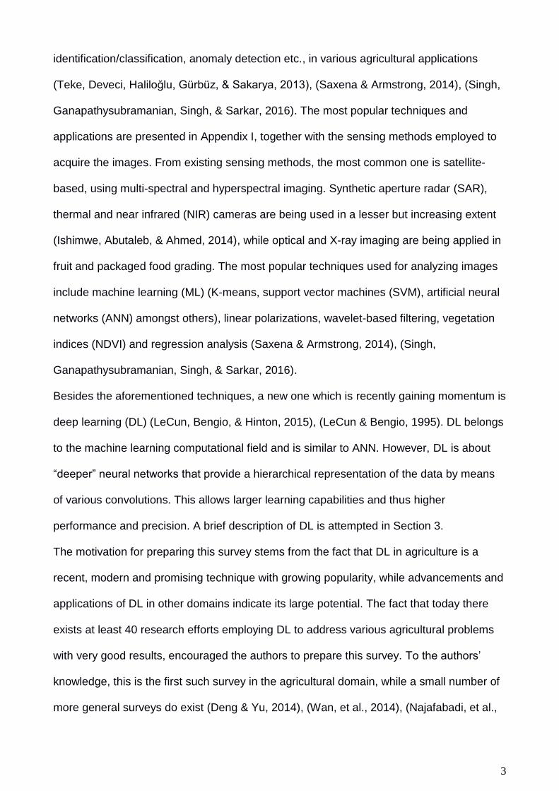
G., Cao, Parsons, Gauss, & Wathes, 2012). An example DL architecture is displayed in
Figure 1, illustrating CaffeNet (Jia, et al., 2014), an example of a convolutional neural
network, combining convolutional and fully connected (dense) layers.

6
Figure 1: CaffeNet, an example CNN architecture. Source: (Sladojevic, Arsenovic, Anderla,
Culibrk, & Stefanovic, 2016)
Convolutional Neural Networks (CNN) constitute a class of deep, feed-forward ANN, and
they appear in numerous of the surveyed papers as the technique used (17 papers, 42%).
As the figure shows, various convolutions are performed at some layers of the network,
creating different representations of the learning dataset, starting from more general ones
at the first larger layers, becoming more specific at the deeper layers. The convolutional
layers act as feature extractors from the input images whose dimensionality is then
reduced by the pooling layers. The convolutional layers encode multiple lower-level
features into more discriminative features, in a way that is spatially context-aware. They
may be understood as banks of filters that transform an input image into another,
highlighting specific patterns. The fully connected layers, placed in many cases near the
output of the model, act as classifiers exploiting the high-level features learned to classify
input images in predefined classes or to make numerical predictions. They take a vector
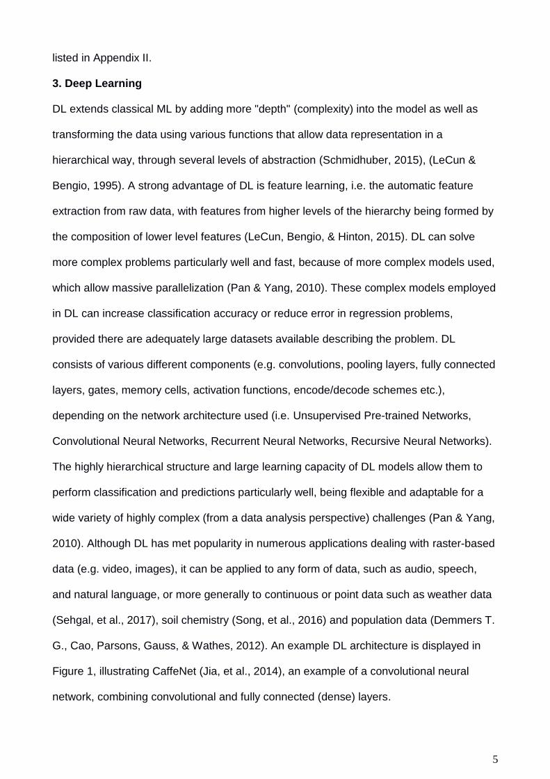
as input and produce another vector as output. An example visualization of leaf images
after each processing step of the CaffeNet CNN, at a problem of identifying plant diseases,
is depicted in Figure 2. We can observe that after each processing step, the particular
elements of the image that reveal the indication of a disease become more evident,
especially at the final step (Pool5).

7
Figure 2: Visualization of the output layers images after each processing step of the CaffeNet CNN
(i.e. convolution, pooling, normalization) at a plant disease identification problem based on leaf
images. Source: (Sladojevic, Arsenovic, Anderla, Culibrk, & Stefanovic, 2016)
One of the most important advantages of using DL in image processing is the reduced
need of feature engineering (FE). Previously, traditional approaches for image
classification tasks had been based on hand-engineered features, whose performance
affected heavily the overall results. FE is a complex, time-consuming process which needs
to be altered whenever the problem or the dataset changes. Thus, FE constitutes an
expensive effort that depends on experts’ knowledge and does not generalize well (Amara,
Bouaziz, & Algergawy, 2017). On the other hand, DL does not require FE, locating the
important features itself through training.
A disadvantage of DL is the generally longer training time. However, testing time is
generally faster than other methods ML-based methods (Chen, Lin, Zhao, Wang, & Gu,
2014). Other disadvantages include problems that might occur when using pre-trained
models on datasets that are small or significantly different, optimization issues because of
the models’ complexity, as well as hardware restrictions.
In Section 5, we discuss over advantages and disadvantages of DL as they reveal through
the surveyed papers.
8
3.1 Available Architectures, Datasets and Tools
There exist various successful and popular architectures, which researchers may use to
start building their models instead of starting from scratch. These include AlexNet
(Krizhevsky, Sutskever, & Hinton, 2012), CaffeNet (Jia, et al., 2014) (displayed in Figure
1), VGG (Simonyan & Zisserman, 2014), GoogleNet (Szegedy, et al., 2015) and Inception-
ResNet (Szegedy, Ioffe, Vanhoucke, & Alemi, 2017), among others. Each architecture has
different advantages and scenarios where it is more appropriate to be used (Canziani,
Paszke, & Culurciello, 2016). It is also worth noting that almost all of the aforementioned
models come along with their weights pre-trained, which means that their network had
been already trained by some dataset and has thus learned to provide accurate
classification for some particular problem domain (Pan & Yang, 2010). Common datasets
used for pre-training DL architectures include ImageNet (Deng, et al., 2009) and PASCAL
VOC (PASCAL VOC Project, 2012) (see also Appendix III).
Moreover, there exist various tools and platforms allowing researchers to experiment with
DL (Bahrampour, Ramakrishnan, Schott, & Shah, 2015). The most popular ones are
Theano, TensorFlow, Keras (which is an application programmer's interface on top of
Theano and TensorFlow), Caffe, PyTorch, TFLearn, Pylearn2 and the Deep Learning
Matlab Toolbox. Some of these tools (i.e. Theano, Caffe) incorporate popular architectures
such as the ones mentioned above (i.e. AlexNet, VGG, GoogleNet), either as libraries or
classes. For a more elaborate description of the DL concept and its applications, the
reader could refer to existing bibliography (Schmidhuber, 2015), (Deng & Yu, 2014), (Wan,
et al., 2014), (Najafabadi, et al., 2015), (Canziani, Paszke, & Culurciello, 2016),
(Bahrampour, Ramakrishnan, Schott, & Shah, 2015).
4. Deep Learning Applications in Agriculture
In Appendix II, we list the 40 identified relevant works, indicating the agricultural-related

9
research area, the particular problem they address, DL models and architectures
implemented, sources of data used, classes and labels of the data, data pre-processing
and/or augmentation employed, overall performance achieved according to the metrics
adopted, as well as comparisons with other techniques, wherever available.
4.1 Areas of Use
Sixteen areas have been identified in total, with the popular ones being identification of
weeds (5 papers), land cover classification (4 papers), plant recognition (4 papers), fruits
counting (4 papers) and crop type classification (4 papers).
It is remarkable that all papers, except from (Demmers T. G., et al., 2010), (Demmers T.
G., Cao, Parsons, Gauss, & Wathes, 2012) and (Chen, Lin, Zhao, Wang, & Gu, 2014),
were published during or after 2015, indicating how recent and modern this technique is, in
the domain of agriculture. More precisely, from the remaining 37 papers, 15 papers have
been published in 2017, 15 in 2016 and 7 in 2015.
The large majority of the papers deal with image classification and identification of areas of
interest, including detection of obstacles (e.g. (Steen, Christiansen, Karstoft, & Jørgensen,
2016), (Christiansen, Nielsen, Steen, Jørgensen, & Karstoft, 2016)) and fruit counting (e.g.
(Rahnemoonfar & Sheppard, 2017), (Sa, et al., 2016)). Some papers focus on predicting
future parameters, such as corn yield (Kuwata & Shibasaki, 2015) soil moisture content at
the field (Song, et al., 2016) and weather conditions (Sehgal, et al., 2017).
From another perspective, most papers (20) target crops, while few works consider issues
such as weed detection (8 papers), land cover (4 papers), research on soil (2 papers),
livestock agriculture (3 papers), obstacle detection (3 papers) and weather prediction (1
paper).
4.2 Data Sources
Observing the sources of data used to train the DL model at every paper, large datasets of
images are mainly used, containing thousands of images in some cases, either real ones
10
(e.g. (Mohanty, Hughes, & Salathé, 2016), (Reyes, Caicedo, & Camargo, 2015),
(Dyrmann, Karstoft, & Midtiby, 2016 )), or synthetic produced by the authors
(Rahnemoonfar & Sheppard, 2017), (Dyrmann, Mortensen, Midtiby, & Jørgensen, 2016).
Some datasets originate from well-known and publicly-available datasets such as
PlantVillage, LifeCLEF, MalayaKew, UC Merced and Flavia (see Appendix III), while
others constitute sets of real images collected by the authors for their research needs (e.g.
(Sladojevic, Arsenovic, Anderla, Culibrk, & Stefanovic, 2016), (Bargoti & Underwood,
2016), (Xinshao & Cheng, 2015), (Sørensen, Rasmussen, Nielsen, & Jørgensen, 2017)).
Papers dealing with land cover, crop type classification and yield estimation, as well as
some papers related to weed detection employ a smaller number of images (e.g. tens of
images), produced by UAV (Lu, et al., 2017), (Rebetez, J., et al., 2016), (Milioto, Lottes, &
Stachniss, 2017), airborne (Chen, Lin, Zhao, Wang, & Gu, 2014), (Luus, Salmon, van den
Bergh, & Maharaj, 2015) or satellite-based remote sensing (Kussul, Lavreniuk, Skakun, &
Shelestov, 2017), (Minh, et al., 2017), (Ienco, Gaetano, Dupaquier, & Maurel, 2017),
(Rußwurm & Körner, 2017). A particular paper investigating segmentation of root and soil
uses images from X-ray tomography (Douarre, Schielein, Frindel, Gerth, & Rousseau,
2016). Moreover, some papers use text data, collected either from repositories (Kuwata &
Shibasaki, 2015), (Sehgal, et al., 2017) or field sensors (Song, et al., 2016), (Demmers T.
G., et al., 2010), (Demmers T. G., Cao, Parsons, Gauss, & Wathes, 2012). In general, the
more complicated the problem to be solved, the more data is required. For example,
problems involving large number of classes to identify (Mohanty, Hughes, & Salathé,
2016), (Reyes, Caicedo, & Camargo, 2015), (Xinshao & Cheng, 2015) and/or small
Variation among the classes (Luus, Salmon, van den Bergh, & Maharaj, 2015), (Rußwurm
& Körner, 2017), (Yalcin, 2017 ), (Namin, Esmaeilzadeh, Najafi, Brown, & Borevitz, 2017),
(Xinshao & Cheng, 2015), require large number of input images to train their models.

11
4.3 Data Variation
Variation between classes is necessary for the DL models to be able to differentiate
features and characteristics, and perform accurate classifications3. Hence, accuracy is
positively correlated with variation among classes. Nineteen papers (47%) revealed some
aspects of poor data variation. Luus et al. (Luus, Salmon, van den Bergh, & Maharaj,
2015) observed high relevance between some land cover classes (i.e. medium density
and dense residential, buildings and storage tanks) while Ienko et al. (Ienco, Gaetano,
Dupaquier, & Maurel, 2017) found that tree crops, summer crops and truck farming were
classes highly mixed. A confusion between maize and soybeans was evident in (Kussul,
Lavreniuk, Skakun, & Shelestov, 2017) and variation was low in botanically related crops,
such as meadow, fallow, triticale, wheat, and rye (Rußwurm & Körner, 2017). Moreover,
some particular views of the plants (i.e. flowers and leaf scans) offer different classification
accuracy than branches, stems and photos of the entire plant. A serious issue in plant
phenology recognition is the fact that appearances change very gradually and it is
challenging to distinguish images falling into the growing durations that are in the middle of
two successive stages (Yalcin, 2017 ), (Namin, Esmaeilzadeh, Najafi, Brown, & Borevitz,
2017). A similar issue appears when assessing the quality of vegetative development
(Minh, et al., 2017). Furthermore, in the challenging problem of fruit counting, the models
suffer from high occlusion, depth variation, and uncontrolled illumination, including high
color similarity between fruit/foliage (Chen, et al., 2017), (Bargoti & Underwood, 2016).
Finally, identification of weeds faces issues with respect to lighting, resolution, and soil
type, and small variation between weeds and crops in shape, texture, color and position
(i.e. overlapping) (Dyrmann, Karstoft, & Midtiby, 2016 ), (Xinshao & Cheng, 2015),
(Dyrmann, Jørgensen, & Midtiby, 2017). In the large majority of the papers mentioned
above (except from (Minh, et al., 2017)), this low variation has affected classification
3 Classification accuracy is defined in Section 4.7 and Table 1.

12
accuracy significantly, i.e. more than 5%.
4.4 Data Pre-Processing
The large majority of related work (36 papers, 90%) involved some image pre-processing
steps, before the image or particular characteristics/features/statistics of the image were
fed as an input to the DL model. The most common pre-processing procedure was image
resize (16 papers), in most cases to a smaller size, in order to adapt to the requirements of
the DL model. Sizes of 256x256, 128x128, 96x96 and 60x60 pixels were common. Image
segmentation was also a popular practice (12 papers), either to increase the size of the
dataset (Ienco, Gaetano, Dupaquier, & Maurel, 2017), (Rebetez, J., et al., 2016), (Yalcin,
2017 ) or to facilitate the learning process by highlighting regions of interest (Sladojevic,
Arsenovic, Anderla, Culibrk, & Stefanovic, 2016), (Mohanty, Hughes, & Salathé, 2016),
(Grinblat, Uzal, Larese, & Granitto, 2016), (Sa, et al., 2016), (Dyrmann, Karstoft, & Midtiby,
2016 ), (Potena, Nardi, & Pretto, 2016) or to enable easier data annotation by experts and
volunteers (Chen, et al., 2017), (Bargoti & Underwood, 2016). Background removal
(Mohanty, Hughes, & Salathé, 2016), (McCool, Perez, & Upcroft, 2017), (Milioto, Lottes, &
Stachniss, 2017), foreground pixel extraction (Lee, Chan, Wilkin, & Remagnino, 2015) or
non-green pixels removal based on NDVI masks (Dyrmann, Karstoft, & Midtiby, 2016 ),
(Potena, Nardi, & Pretto, 2016) were also performed to reduce the datasets’ overall noise.
Other operations involved the creation of bounding boxes (Chen, et al., 2017), (Sa, et al.,
2016), (McCool, Perez, & Upcroft, 2017), (Milioto, Lottes, & Stachniss, 2017) to facilitate
detection of weeds or counting of fruits. Some datasets were converted to grayscale
(Santoni, Sensuse, Arymurthy, & Fanany, 2015), (Amara, Bouaziz, & Algergawy, 2017) or
to the HSV color model (Luus, Salmon, van den Bergh, & Maharaj, 2015), (Lee, Chan,
Wilkin, & Remagnino, 2015).
Furthermore, some papers used features extracted from the images as input to their
models, such as shape and statistical features (Hall, McCool, Dayoub, Sunderhauf, &

13
Upcroft, 2015), histograms (Hall, McCool, Dayoub, Sunderhauf, & Upcroft, 2015), (Xinshao
& Cheng, 2015), (Rebetez, J., et al., 2016), Principal Component Analysis (PCA) filters
(Xinshao & Cheng, 2015), Wavelet transformations (Kuwata & Shibasaki, 2015) and Gray
Level Co-occurrence Matrix (GLCM) features (Santoni, Sensuse, Arymurthy, & Fanany,
2015). Satellite or aerial images involved a combination of pre-processing steps such as
orthorectification (Lu, et al., 2017), (Minh, et al., 2017) calibration and terrain correction
(Kussul, Lavreniuk, Skakun, & Shelestov, 2017), (Minh, et al., 2017) and atmospheric
correction (Rußwurm & Körner, 2017).
4.5 Data Augmentation
It is worth-mentioning that some of the related work under study (15 papers, 37%)
employed data augmentation techniques (Krizhevsky, Sutskever, & Hinton, 2012), to
enlarge artificially their number of training images. This helps to improve the overall
learning procedure and performance, and for generalization purposes, by means of
feeding the model with varied data. This augmentation process is important for papers that
possess only small datasets to train their DL models, such as (Bargoti & Underwood,
2016), (Sladojevic, Arsenovic, Anderla, Culibrk, & Stefanovic, 2016), (Sørensen,
Rasmussen, Nielsen, & Jørgensen, 2017), (Mortensen, Dyrmann, Karstoft, Jørgensen, &
Gislum, 2016), (Namin, Esmaeilzadeh, Najafi, Brown, & Borevitz, 2017) and (Chen, et al.,
2017). This process was especially important in papers where the authors trained their
models using synthetic images and tested them on real ones (Rahnemoonfar & Sheppard,
2017) and (Dyrmann, Mortensen, Midtiby, & Jørgensen, 2016). In this case, data
augmentation allowed their models to generalize and be able to adapt to the real-world
problems more easily.
Transformations are label-preserving, and included rotations (12 papers), dataset
partitioning/cropping (3 papers), scaling (3 papers), transposing (Sørensen, Rasmussen,
Nielsen, & Jørgensen, 2017), mirroring (Dyrmann, Karstoft, & Midtiby, 2016 ), translations

14
and perspective transform (Sladojevic, Arsenovic, Anderla, Culibrk, & Stefanovic, 2016),
adaptations of objects’ intensity in an object detection problem (Steen, Christiansen,
Karstoft, & Jørgensen, 2016) and a PCA augmentation technique (Bargoti & Underwood,
2016).
Papers involving simulated data performed additional augmentation techniques such as
varying the HSV channels and adding random shadows (Dyrmann, Mortensen, Midtiby, &
Jørgensen, 2016) or adding simulated roots to soil images (Douarre, Schielein, Frindel,
Gerth, & Rousseau, 2016).
4.6 Technical Details
From a technical side, almost half of the research works (17 papers, 42%) employed
popular CNN architectures such as AlexNet, VGG16 and Inception-ResNet. From the rest,
14 papers developed their own CNN models, 2 papers adopted a first-order Differential
Recurrent Neural Networks (DRNN) model, 5 papers preferred to use a Long Short-Term
Memory (LSTM) model (Gers, Schmidhuber, & Cummins, 2000), one paper used deep
belief networks (DBN) and one paper employed a hybrid of PCA with auto-encoders (AE).
Some of the CNN approaches combined their model with a classifier at the output layer,
such as logistic regression (Chen, Lin, Zhao, Wang, & Gu, 2014), Scalable Vector
Machines (SVM) (Douarre, Schielein, Frindel, Gerth, & Rousseau, 2016), linear regression
(Chen, et al., 2017), Large Margin Classifiers (LCM) (Xinshao & Cheng, 2015) and
macroscopic cellular automata (Song, et al., 2016).
Regarding the frameworks used, all the works that employed some well-known CNN
architecture had also used a DL framework, with Caffe being the most popular (13 papers,
32%), followed by Tensor Flow (2 papers) and deeplearning4j (1 paper). Ten research
works developed their own software, while some authors decided to build their own
models on top of Caffe (5 papers), Keras/Theano (5 papers), Keras/TensorFlow (4
papers), Pylearn2 (1 paper), MatConvNet (1 paper) and Deep Learning Matlab Toolbox (1

15
paper). A possible reason for the wide use of Caffe is that it incorporates various CNN
frameworks and datasets, which can be used then easily and automatically by its users.
Most of the studies divided their dataset between training and testing/verification data
using a ratio of 80-20 or 90-10 respectively. In addition, various learning rates have been
recorded, from 0.001 (Amara, Bouaziz, & Algergawy, 2017) and 0.005 (Mohanty, Hughes,
& Salathé, 2016) up to 0.01 (Grinblat, Uzal, Larese, & Granitto, 2016). Learning rate is
about how quickly a network learns. Higher values help avoid the solver being stuck in
local minima, which can reduce performance significantly. A general approach used by
many of the evaluated papers is to start out with a high learning rate and lower it as the
training goes on. We note that learning rate is very dependent on the network architecture.
Moreover, most of the research works that incorporated popular DL architectures took
advantage of transfer learning (Pan & Yang, 2010), which concerns leveraging the already
existing knowledge of some related task or domain in order to increase the learning
efficiency of the problem under study by fine-tuning pre-trained models. As sometimes it is
not possible to train a network from scratch due to having a small training data set or
having a complex multi-task network, it is required that the network be at least partially
initialized with weights from another pre-trained model. A common transfer learning
technique is the use of pre-trained CNN, which are CNN models that have been already
trained on some relevant dataset with possibly different number of classes. These models
are then adapted to the particular challenge and dataset. This method was followed
(among others) in (Lu, et al., 2017), (Douarre, Schielein, Frindel, Gerth, & Rousseau,
2016), (Reyes, Caicedo, & Camargo, 2015), (Bargoti & Underwood, 2016), (Steen,
Christiansen, Karstoft, & Jørgensen, 2016), (Lee, Chan, Wilkin, & Remagnino, 2015), (Sa,
et al., 2016), (Mohanty, Hughes, & Salathé, 2016), (Christiansen, Nielsen, Steen,
Jørgensen, & Karstoft, 2016), (Sørensen, Rasmussen, Nielsen, & Jørgensen, 2017), for
the VGG16, DenseNet, AlexNet and GoogleNet architectures.

16
4.7 Outputs
Finally, concerning the 31 papers that involved classification, the classes as used by the
authors ranged from 2 (Lu, et al., 2017), (Pound, M. P., et al., 2016), (Douarre, Schielein,
Frindel, Gerth, & Rousseau, 2016), (Milioto, Lottes, & Stachniss, 2017) up to 1,000
(Reyes, Caicedo, & Camargo, 2015). A large number of classes was observed in (Luus,
Salmon, van den Bergh, & Maharaj, 2015) (21 land-use classes), (Rebetez, J., et al.,
2016) (22 different crops plus soil), (Lee, Chan, Wilkin, & Remagnino, 2015) (44 plant
species) and (Xinshao & Cheng, 2015) (91 classes of common weeds found in agricultural
fields). In these papers, the number of outputs of the model was equal to the number of
classes respectively. Each output was a different probability for the input image, segment,
blob or pixel to belong to each class, and then the model picked the highest probability as
its predicted class.
From the rest 9 papers, 2 performed predictions of fruits counted (scalar value as output)
(Rahnemoonfar & Sheppard, 2017), (Chen, et al., 2017), 2 identified regions of fruits in the
image (multiple bounding boxes) (Bargoti & Underwood, 2016), (Sa, et al., 2016), 2
predicted animal growth (scalar value) (Demmers T. G., et al., 2010), (Demmers T. G.,
Cao, Parsons, Gauss, & Wathes, 2012), one predicted weather conditions (scalar value)
(Sehgal, et al., 2017), one crop yield index (scalar value) (Kuwata & Shibasaki, 2015) and
one paper predicted percentage of soil moisture content (scalar value) (Song, et al., 2016).
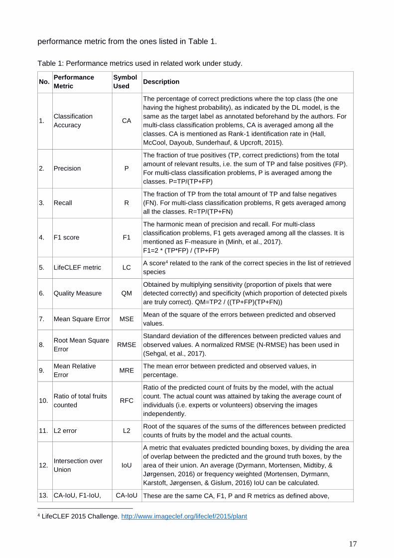
4.8 Performance Metrics
Regarding methods used to evaluate performance, various metrics have been employed
by the authors, each being specific to the model used at each study. Table 1 lists these
metrics, together with their definition/description, and the symbol we use to refer to them in
this survey. In some papers where the authors referred to accuracy without specifying its
definition, we assumed they referred to classification accuracy (CA, first metric listed in
Table 1). From this point onwards, we refer to “DL performance” as its score in some
17
performance metric from the ones listed in Table 1.
Table 1: Performance metrics used in related work under study.
No. Performance
Metric Symbol
Used Description
1. Classification
Accuracy CA
The percentage of correct predictions where the top class (the one
having the highest probability), as indicated by the DL model, is the
same as the target label as annotated beforehand by the authors. For
multi-class classification problems, CA is averaged among all the
classes. CA is mentioned as Rank-1 identification rate in (Hall,
McCool, Dayoub, Sunderhauf, & Upcroft, 2015).
2. Precision P
The fraction of true positives (TP, correct predictions) from the total
amount of relevant results, i.e. the sum of TP and false positives (FP).
For multi-class classification problems, P is averaged among the
classes. P=TP/(TP+FP)
3. Recall R
The fraction of TP from the total amount of TP and false negatives
(FN). For multi-class classification problems, R gets averaged among
all the classes. R=TP/(TP+FN)
4. F1 score F1
The harmonic mean of precision and recall. For multi-class
classification problems, F1 gets averaged among all the classes. It is
mentioned as F-measure in (Minh, et al., 2017).
F1=2 * (TP*FP) / (TP+FP)
5. LifeCLEF metric LC A score4 related to the rank of the correct species in the list of retrieved
species
6. Quality Measure QM
Obtained by multiplying sensitivity (proportion of pixels that were
detected correctly) and specificity (which proportion of detected pixels
are truly correct). QM=TP2 / ((TP+FP)(TP+FN))
7. Mean Square Error MSE Mean of the square of the errors between predicted and observed
values.
8. Root Mean Square
Error RMSE
Standard deviation of the differences between predicted values and
observed values. A normalized RMSE (N-RMSE) has been used in
(Sehgal, et al., 2017).
9. Mean Relative
Error MRE
The mean error between predicted and observed values, in
percentage.
10. Ratio of total fruits
counted RFC
Ratio of the predicted count of fruits by the model, with the actual
count. The actual count was attained by taking the average count of
individuals (i.e. experts or volunteers) observing the images
independently.
11. L2 error L2 Root of the squares of the sums of the differences between predicted
counts of fruits by the model and the actual counts.
12. Intersection over
Union IoU
A metric that evaluates predicted bounding boxes, by dividing the area
of overlap between the predicted and the ground truth boxes, by the
area of their union. An average (Dyrmann, Mortensen, Midtiby, &
Jørgensen, 2016) or frequency weighted (Mortensen, Dyrmann,
Karstoft, Jørgensen, & Gislum, 2016) IoU can be calculated.
13. CA-IoU, F1-IoU, CA-IoU These are the same CA, F1, P and R metrics as defined above,
4 LifeCLEF 2015 Challenge. http://www.imageclef.org/lifeclef/2015/plant
18
P-IoU or R-IoU F1-IoU
P-IoU
R-IoU
combined with IoU in order to consider true/false positives/negatives. Used in problems involving bounding boxes. This is done by putting a minimum threshold on IoU, i.e. any value above this threshold would be considered as positive by the metric (and the model involved). Thresholds of 20% (Bargoti & Underwood, 2016), 40% (Sa, et al., 2016) and 50% (Steen, Christiansen, Karstoft, & Jørgensen, 2016), (Christiansen, Nielsen, Steen, Jørgensen, & Karstoft, 2016), (Dyrmann, Jørgensen, & Midtiby, 2017) have been observed5.
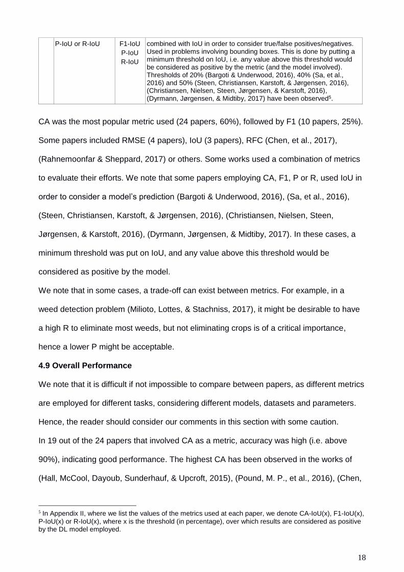
CA was the most popular metric used (24 papers, 60%), followed by F1 (10 papers, 25%).
Some papers included RMSE (4 papers), IoU (3 papers), RFC (Chen, et al., 2017),
(Rahnemoonfar & Sheppard, 2017) or others. Some works used a combination of metrics
to evaluate their efforts. We note that some papers employing CA, F1, P or R, used IoU in
order to consider a model’s prediction (Bargoti & Underwood, 2016), (Sa, et al., 2016),
(Steen, Christiansen, Karstoft, & Jørgensen, 2016), (Christiansen, Nielsen, Steen,
Jørgensen, & Karstoft, 2016), (Dyrmann, Jørgensen, & Midtiby, 2017). In these cases, a
minimum threshold was put on IoU, and any value above this threshold would be
considered as positive by the model.
We note that in some cases, a trade-off can exist between metrics. For example, in a
weed detection problem (Milioto, Lottes, & Stachniss, 2017), it might be desirable to have
a high R to eliminate most weeds, but not eliminating crops is of a critical importance,
hence a lower P might be acceptable.
4.9 Overall Performance
We note that it is difficult if not impossible to compare between papers, as different metrics
are employed for different tasks, considering different models, datasets and parameters.
Hence, the reader should consider our comments in this section with some caution.
In 19 out of the 24 papers that involved CA as a metric, accuracy was high (i.e. above
90%), indicating good performance. The highest CA has been observed in the works of
(Hall, McCool, Dayoub, Sunderhauf, & Upcroft, 2015), (Pound, M. P., et al., 2016), (Chen,
5 In Appendix II, where we list the values of the metrics used at each paper, we denote CA-IoU(x), F1-IoU(x),
P-IoU(x) or R-IoU(x), where x is the threshold (in percentage), over which results are considered as positive by the DL model employed.
19
Lin, Zhao, Wang, & Gu, 2014), (Lee, Chan, Wilkin, & Remagnino, 2015), (Minh, et al.,
2017), (Potena, Nardi, & Pretto, 2016) and (Steen, Christiansen, Karstoft, & Jørgensen,
2016), with values of 98% or more, constituting remarkable results. From the 10 papers
using F1 as metric, 5 had values higher than 0.90 with the highest F1 observed in
(Mohanty, Hughes, & Salathé, 2016) and (Minh, et al., 2017) with values higher than 0.99.
The works of (Dyrmann, Karstoft, & Midtiby, 2016 ), (Rußwurm & Körner, 2017), (Ienco,
Gaetano, Dupaquier, & Maurel, 2017), (Mortensen, Dyrmann, Karstoft, Jørgensen, &
Gislum, 2016), (Rebetez, J., et al., 2016), (Christiansen, Nielsen, Steen, Jørgensen, &
Karstoft, 2016) and (Yalcin, 2017 ) were among the ones with the lowest CA (i.e. 73-79%)
and/or F1 scores (i.e. 0.558 - 0.746), however state of the art work in these particular
problems has shown lower CA (i.e. SVM, RF, Naïve- Bayes classifier). Particularly in
(Rußwurm & Körner, 2017), the three-unit LSTM model employed provided 16.3% better
CA than a CNN, which belongs to the family of DL. Besides, the above can be considered
as “harder” problems, because of the use of satellite data (Ienco, Gaetano, Dupaquier, &
Maurel, 2017), (Rußwurm & Körner, 2017) large number of classes (Dyrmann, Karstoft, &
Midtiby, 2016 ), (Rußwurm & Körner, 2017), (Rebetez, J., et al., 2016), small training
datasets (Mortensen, Dyrmann, Karstoft, Jørgensen, & Gislum, 2016), (Christiansen,
Nielsen, Steen, Jørgensen, & Karstoft, 2016) or very low variation among the classes
(Yalcin, 2017 ), (Dyrmann, Karstoft, & Midtiby, 2016 ), (Rebetez, J., et al., 2016).
4.10 Generalizations on Different Datasets
It is important to examine whether the authors had tested their implementations on the
same dataset (e.g. by dividing the dataset into training and testing/validation sets) or used
different datasets to test their solution. From the 40 papers, only 8 (20%) used different
datasets for testing than the one for training. From these, 2 approaches trained their
models by using simulated data and tested on real data (Dyrmann, Mortensen, Midtiby, &
Jørgensen, 2016), (Rahnemoonfar & Sheppard, 2017) and 2 papers tested their models
20
on a dataset produced 2-4 weeks after, with a more advanced growth stage of plants and
weeds (Milioto, Lottes, & Stachniss, 2017), (Potena, Nardi, & Pretto, 2016). Moreover, 3
papers used different fields for testing than the ones used for training (McCool, Perez, &
Upcroft, 2017), with a severe degree of occlusion compared to the other training field
(Dyrmann, Jørgensen, & Midtiby, 2017), or containing other obstacles such as people and
animals (Steen, Christiansen, Karstoft, & Jørgensen, 2016). Sa et al. (Sa, et al., 2016)
used a different dataset to evaluate whether the model can generalize on different fruits.
From the other 32 papers, different trees were used in training and testing in (Chen, et al.,
2017), while different rooms for pigs (Demmers T. G., Cao, Parsons, Gauss, & Wathes,
2012) and chicken (Demmers T. G., et al., 2010) were considered. Moreover, Hall et al.
applied condition variations in testing (i.e. translations, scaling, rotations, shading and
occlusions) (Hall, McCool, Dayoub, Sunderhauf, & Upcroft, 2015) while scaling for a
certain range translation distance and rotation angle was performed on the testing dataset
in (Xinshao & Cheng, 2015). The rest 27 papers did not perform any changes between the
training/testing datasets, a fact that lowers the overall confidence for the results presented.
Finally, it is interesting to observe how these generalizations affected the performance of
the models, at least in cases where both data from same and different datasets were used
in testing. In (Sa, et al., 2016), F1-IoU(40) was higher for the detection of apples (0.938),
strawberry (0.948), avocado (0.932) and mango (0.942), than in the default case of sweet
pepper (0.838). In (Rahnemoonfar & Sheppard, 2017), RFC was 2% less in the real
images than in the synthetic ones. In (Potena, Nardi, & Pretto, 2016), CA was 37.6% less
at the dataset involving plants of 4-weeks more advanced growth. According to the
authors, the model was trained based on plants that were in their first growth stage, thus
without their complete morphological features, which were included in the testing dataset.
Moreover, in (Milioto, Lottes, & Stachniss, 2017) P was 2% higher at the 2-weeks more
advanced growth dataset, with 9% lower R.

21
Hence, in the first case there was improvement in performance (Sa, et al., 2016), and in
the last three cases a reduction, slight one in (Rahnemoonfar & Sheppard, 2017) and
(Milioto, Lottes, & Stachniss, 2017) but considerable in (Potena, Nardi, & Pretto, 2016).
From the other papers using different testing datasets, as mentioned above, high
percentages of CA (94-97.3%), P-IoU (86.6%) and low values of MRE (1.8 -10%) have
been reported. These show that the DL models were able to generalize well to different
datasets. However, without more comparisons, this is only a speculation that can be
figured out of the small number of observations available.
4.11 Performance Comparison with Other Approaches
A critical aspect of this survey is to examine how DL performs in relation to other existing
techniques. The 14th column of Appendix II presents whether the authors of related work
compared their DL-based approach with other techniques used for solving their problem
under study. We focus only on comparisons between techniques used for the same
dataset at the same research paper, with the same metric.
In almost all cases, the DL models outperform other approaches implemented for
comparison purposes. CNN show 1-8% higher CA in comparison to SVM (Chen, Lin,
Zhao, Wang, & Gu, 2014), (Lee, Chan, Wilkin, & Remagnino, 2015), (Grinblat, Uzal,
Larese, & Granitto, 2016), (Pound, M. P., et al., 2016), 41% improvement of CA when
compared to ANN (Lee, Chan, Wilkin, & Remagnino, 2015) and 3-8% higher CA when
compared to RF (Kussul, Lavreniuk, Skakun, & Shelestov, 2017), (Minh, et al., 2017),
(McCool, Perez, & Upcroft, 2017), (Potena, Nardi, & Pretto, 2016), (Hall, McCool, Dayoub,
Sunderhauf, & Upcroft, 2015). CNN also seem to be superior than unsupervised feature
learning with 3-11% higher CA (Luus, Salmon, van den Bergh, & Maharaj, 2015), 2-44%
improved CA in relation to local shape and color features (Dyrmann, Karstoft, & Midtiby,
2016 ), (Sørensen, Rasmussen, Nielsen, & Jørgensen, 2017), and 2% better CA (Kussul,
Lavreniuk, Skakun, & Shelestov, 2017) or 18% less RMSE (Song, et al., 2016) compared
22
to multilayer perceptrons. CNN had also superior performance than Penalized
Discriminant Analysis (Grinblat, Uzal, Larese, & Granitto, 2016), SVM Regression (Kuwata
& Shibasaki, 2015), area-based techniques (Rahnemoonfar & Sheppard, 2017), texture-
based regression models (Chen, et al., 2017), LMC classifiers (Xinshao & Cheng, 2015),
Gaussian Mixture Models (Santoni, Sensuse, Arymurthy, & Fanany, 2015) and Naïve-
Bayes classifiers (Yalcin, 2017 ).
In cases where Recurrent Neural Networks (RNN) (Mandic & Chambers, 2001)
architectures were employed, the LSTM model had 1% higher CA than RF and SVM in
(Ienco, Gaetano, Dupaquier, & Maurel, 2017), 44% improved CA than SVM in (Rußwurm
& Körner, 2017) and 7-9% better CA than RF and SVM in (Minh, et al., 2017).
In only one case, DL showed worse performance against another technique, and this was
when a CNN was compared to an approach involving local descriptors to represent
images together with KNN as the classification strategy (20% worse LC) (Reyes, Caicedo,
& Camargo, 2015).
5. Discussion
Our analysis has shown that DL offers superior performance in the vast majority of related
work. When comparing the performance of DL-based approaches with other techniques at
each paper, it is of paramount importance to adhere to the same experimental conditions
(i.e. datasets and performance metrics). From the related work under study, 28 out of the
40 papers (70%) performed direct, valid and correct comparisons among the DL-based
approach employed and other state-of-art techniques used to solve the particular problem
tackled at each paper. Due to the fact that each paper involved different datasets, pre-
processing techniques, metrics, models and parameters, it is difficult if not impossible to
generalize and perform comparisons between papers. Thus, our comparisons have been
strictly limited among the techniques used at each paper. Thus, based on these
23
constraints, we have observed that DL has outperformed traditional approaches used such
as SVM, RF, ANN, LMC classifiers and others. It seems that the automatic feature
extraction performed by DL models is more effective than the feature extraction process
through traditional approaches such as Scale Invariant Feature Transform (SIFT), GLCM,
histograms, area-based techniques (ABT), statistics-, texture-, color- and shape-based
algorithms, conditional random fields to model color and visual texture features, local de-
correlated channel features and other manual feature extraction techniques. This is
reinforced by the combined CNN+LSTM model employed in (Namin, Esmaeilzadeh, Najafi,
Brown, & Borevitz, 2017), which outperformed a LSTM model which used hand crafted
feature descriptors as inputs by 25% higher CA. Interesting attempts to combine hand-
crafted features and CNN-based features were performed in (Hall, McCool, Dayoub,
Sunderhauf, & Upcroft, 2015) and (Rebetez, J., et al., 2016).
Although DL has been associated with computer vision and image analysis (which is also
the general case in this survey), we have observed 5 related works where DL-based
models have been trained based on field sensory data (Kuwata & Shibasaki, 2015),
(Sehgal, et al., 2017) and a combination of static and dynamic environmental variables
(Song, et al., 2016), (Demmers T. G., et al., 2010), (Demmers T. G., Cao, Parsons, Gauss,
& Wathes, 2012). These papers indicate the potential of DL to be applied in a wide variety
of agricultural problems, not only those involving images.
Examining agricultural areas where DL techniques have been applied, leaf classification,
leaf and plant disease detection, plant recognition and fruit counting have some papers
which present very good performance (i.e. CA > 95%, F1 > 0.92 or RFC > 0.9). This is
probably because of the availability of datasets in these domains, as well as the distinct
characteristics of (sick) leaves/plants and fruits in the image. On the other hand, some
papers in land cover classification, crop type classification, plant phenology recognition
and weed detection showed average performance (i.e. CA < 87% or F1 < 0.8). This could
24
be due to leaf occlusion in weed detection, use of noise-prone satellite imagery in land
cover problems, crops with low variation and botanical relationship or the fact that
appearances change very gradually while plants grow in phenology recognition efforts.
Without underestimating the quality of any of the surveyed papers, we highlight some that
claim high performance (CA > 91%, F1-IoU(20) > 0.90 or RFC > 0.91), considering the
complexity of the problem in terms of its definition or the large number of classes involved
(more than 21 classes). These papers are the following: (Mohanty, Hughes, & Salathé,
2016), (Luus, Salmon, van den Bergh, & Maharaj, 2015), (Lee, Chan, Wilkin, &
Remagnino, 2015), (Rahnemoonfar & Sheppard, 2017), (Chen, et al., 2017), (Bargoti &
Underwood, 2016), (Xinshao & Cheng, 2015) and (Hall, McCool, Dayoub, Sunderhauf, &
Upcroft, 2015). We also highlight papers that trained their models on simulated data, and
tested them on real data, which are (Dyrmann, Mortensen, Midtiby, & Jørgensen, 2016),
(Rahnemoonfar & Sheppard, 2017), and (Douarre, Schielein, Frindel, Gerth, & Rousseau,
2016). These works constitute important efforts in the DL community, as they attempt to
solve the problem of inexistent or not large enough datasets in various problems.
Finally, as discussed in Section 4.10, most authors used the same datasets for training
and testing their implementation, a fact that lowers the confidence in the overall findings,
although there have been indications that the models seem to generalize well, with only
small reductions in performance.
5.1 Advanced Deep Learning Applications
Although the majority of papers used typical CNN architectures to perform classification
(23 papers, 57%), some authors experimented with more advanced models in order to
solve more complex problems, such as crop type classification from UAV imagery (CNN +
HistNN using RGB histograms) (Rebetez, J., et al., 2016), estimating number of tomato
fruits (Modified Inception-ResNet CNN) (Rahnemoonfar & Sheppard, 2017) and estimating
number of orange or apple fruits (CNN adapted for blob detection and counting + Linear
25
Regression) (Chen, et al., 2017). Particularly interesting were the approaches employing
the Faster Region-based CNN + VGG16 model (Bargoti & Underwood, 2016), (Sa, et al.,
2016), in order not only to count fruits and vegetables, but also to locate their placement in
the image by means of bounding boxes. Similarly, the work in (Dyrmann, Jørgensen, &
Midtiby, 2017) used the DetectNet CNN to detect bounding boxes of weed instances in
images of cereal fields. These approaches (Faster Region-based CNN, DetectNet CNN)
constitute a very promising research direction, since the task of identifying the bounding
box of fruits/vegetables/weeds in an image has numerous real-life applications and could
solve various agricultural problems
Moreover, considering not only space but also time series, some authors employed RNN-
based models in land cover classification (one-unit LSTM model + SVM) (Ienco, Gaetano,
Dupaquier, & Maurel, 2017), crop type classification (three-unit LSTM) (Rußwurm &
Körner, 2017), classification of different accessions of Arabidopsis thaliana based on
successive top-view images (CNN+ LSTM) (Namin, Esmaeilzadeh, Najafi, Brown, &
Borevitz, 2017), mapping winter vegetation quality coverage (Five-unit LSTM, Gated
Recurrent Unit) (Minh, et al., 2017), estimating the weight of pigs or chickens (DRNN)
(Demmers T. G., et al., 2010), (Demmers T. G., Cao, Parsons, Gauss, & Wathes, 2012)
and for predicting weather based on previous year’s conditions (LSTM) (Sehgal, et al.,
2017). RNN-based models offer higher performance, as they can capture the time
dimension, which is impossible to be exploited by simple CNN. RNN architectures tend to
exhibit dynamic temporal behavior, being able to record long-short temporal
dependencies, remembering and forgetting after some time or when needed (i.e. LSTM).
Differences in performance between RNN and CNN are distinct in the related work under
study, as shown in Table 2. This 16% improvement in CA could be attributed to the
additional information provided by the time series. For example, in the crop type
classification case (Rußwurm & Körner, 2017), the authors mention, “crops change their

26
spectral characteristics due to environmental influences and can thus not be monitored
effectively with classical mono-temporal approaches. Performance of temporal models
increases at the beginning of vegetation period”. LSTM-based approaches work well also
for low represented and difficult classes, as demonstrated in (Ienco, Gaetano, Dupaquier,
& Maurel, 2017).
Table 2: Difference in Performance between CNN and RNN.
No. Application in
Agriculture Performan
ce Metric Difference in Performance
Reference
1. Crop type classification
considering time series CA, F1
Three-unit LSTM: 76.2% (CA),
0.558 (F1)
CNN: 59.9% (CA), 0.236 (F1)
(Rußwurm & Körner, 2017)
2.
Classify the phenotyping
of Arabidopsis in four
accessions
CA CNN+ LSTM: 93%
CNN: 76.8%
(Namin, Esmaeilzadeh,
Najafi, Brown, & Borevitz,
2017)
Finally, the critical aspect of fast processing of DL models in order to be easily used in
robots for real-time decision making (e.g. detection of weeds) was examined in (McCool,
Perez, & Upcroft, 2017), and it is worth-mentioning. The authors have showed that a
lightweight implementation had only a small penalty in CA (3.90%), being much faster (i.e.
processing of 40.6 times more pixels per second). They proposed the idea of “teacher and
student networks”, where the teacher is the more heavy approach that helps the student
(light implementation) to learn faster and better.
5.2 Advantages of Deep Learning
Except from improvements in performance of the classification/prediction problems in the
surveyed works (see Sections 4.9 and 4.11), the advantage of DL in terms of reduced
effort in feature engineering was demonstrated in many of the papers. Hand-engineered
components require considerable time, an effort that takes place automatically in DL.
Besides, sometimes manual search for good feature extractors is not an easy and obvious
task. For example, in the case of estimating crop yield (Kuwata & Shibasaki, 2015),
extracting manually features that significantly affected crop growth was not possible. This
27
was also the case of estimating the soil moisture content (Song, et al., 2016).
Moreover, DL models seem to generalize well. For example, in the case of fruit counting,
the model learned explicitly to count (Rahnemoonfar & Sheppard, 2017). In the banana
leaf classification problem (Amara, Bouaziz, & Algergawy, 2017), the model was robust
under challenging conditions such as illumination, complex background, different
resolution, size and orientation of the images. Also in the fruits counting papers (Chen, et
al., 2017), (Rahnemoonfar & Sheppard, 2017), the models were robust to occlusion,
variation, illumination and scale. The same detection frameworks could be used for a
variety of circular fruits such as peaches, citrus, mangoes etc. As another example, a key
feature of the DeepAnomaly model was the ability to detect unknown objects/anomalies
and not just a set of predefined objects, exploiting the homogeneous characteristics of an
agricultural field to detect distant, heavy occluded and unknown objects (Christiansen,
Nielsen, Steen, Jørgensen, & Karstoft, 2016). Moreover, in the 8 papers mentioned in
Section 4.10 where different datasets were used for testing, the performance of the model
was generally high, with only small reductions in performance in comparison with the
performance when using the same dataset for training and testing.
Although DL takes longer time to train than other traditional approaches (e.g. SVM, RF), its
testing time efficiency is quite fast. For example, in detecting obstacles and anomaly
(Christiansen, Nielsen, Steen, Jørgensen, & Karstoft, 2016), the model took much longer
to train, but after it did, its testing time was less than the one of SVM and KNN. Besides, if
we take into account the time needed to manually design filters and extract features, “the
time used on annotating images and training the CNN becomes almost negligible”
(Sørensen, Rasmussen, Nielsen, & Jørgensen, 2017).
Another advantage of DL is the possibility to develop simulated datasets to train the
model, which could be properly designed in order to solve real-world problems. For
example, in the issue of detecting weeds and maize in fields (Dyrmann, Mortensen,

28
Midtiby, & Jørgensen, 2016), the authors overcame the plant foliage overlapping problem
by simulating top-down images of overlapping plants on soil background. The trained
network was then capable of distinguish weeds from maize even in overlapping conditions.
5.3 Disadvantages and Limitations of Deep Learning
A considerable drawback and barrier in the use of DL is the need of large datasets, which
would serve as the input during the training procedure. In spite of data augmentation
techniques which augment some dataset with label-preserving transformations, in reality at
least some hundreds of images are required, depending on the complexity of the problem
under study (i.e. number of classes, precision required etc.). For example, the authors in
(Mohanty, Hughes, & Salathé, 2016) and (Sa, et al., 2016) commented that a more diverse
set of training data was needed to improve CA. A big problem with many datasets is the
low variation among the different classes (Yalcin, 2017 ), as discussed in Section 4.3, or
the existence of noise, in the form of low resolution, inaccuracy of sensory equipment
(Song, et al., 2016), crops’ occlusions, plants overlapping and clustering, and others.
As data annotation is a necessary operation in the large majority of cases, some tasks are
more complex and there is a need for experts (who might be difficult to involve) in order to
annotate input images. As mentioned in (Amara, Bouaziz, & Algergawy, 2017), there is a
limited availability of resources and expertise on banana pathology worldwide. In some
cases, experts or volunteers are susceptible to errors during data labeling, especially when
this is a challenging task e.g. fruit count (Chen, et al., 2017), (Bargoti & Underwood, 2016)
or to determine if images contain weeds or not (Sørensen, Rasmussen, Nielsen, &
Jørgensen, 2017), (Dyrmann, Jørgensen, & Midtiby, 2017).
Another limitation is the fact that the DL models can learn some problem particularly well,
even generalize in some aspects as mentioned in Section 5.2, but they cannot generalize
beyond the “boundaries of the dataset’s expressiveness”. For example, classification of
single leaves, facing up, on a homogeneous background is performed in (Mohanty,

29
Hughes, & Salathé, 2016). A real world application should be able to classify images of a
disease as it presents itself directly on the plant. Many diseases do not present
themselves on the upper side of leaves only. As another example, plant recognition in
(Lee, Chan, Wilkin, & Remagnino, 2015) was noticeably affected by environmental factors
such as wrinkled surface and insect damages. The model for counting tomatoes in
(Rahnemoonfar & Sheppard, 2017) could count ripe and half-ripe fruits, however, “it failed
to count green fruits because it was not trained for this purpose”. If an object size in a
testing image was significantly less than that of a training set, the model missed the
detection in (Sa, et al., 2016). Difficulty in detecting heavily occluded and distant objects
was observed in (Christiansen, Nielsen, Steen, Jørgensen, & Karstoft, 2016). Occlusion
was a serious issue also in (Hall, McCool, Dayoub, Sunderhauf, & Upcroft, 2015).
A general issue in computer vision, not only in DL, is that data pre-processing is
sometimes a necessary and time-consuming task, especially when satellite or aerial
photos are involved, as we saw in Section 4.4. A problem with hyperspectral data is their
high dimensionality and limited training samples (Chen, Lin, Zhao, Wang, & Gu, 2014).
Moreover, sometimes the existing datasets do not describe completely the problem they
target (Song, et al., 2016). As an example, for estimating corn yield (Kuwata & Shibasaki,
2015), it was necessary to consider also external factors other than the weather by
inputting cultivation information such as fertilization and irrigation.
Finally, in the domain of agriculture, there do not exist many publicly available datasets for
researchers to work with, and in many cases, researchers need to develop their own sets
of images. This could require many hours or days of work.
5.4 Future of Deep Learning in Agriculture
Observing Appendix I, which lists various existing applications of computer vision in
agriculture, we can see that only the problems of land cover classification, crop type
estimation, crop phenology, weed detection and fruit grading have been approximated
30
using DL. It is interesting to see how DL would behave also in other agricultural-related
problems listed in Appendix I, such as seeds identification, soil and leaf nitrogen content,
irrigation, plants’ water stress detection, water erosion assessment, pest detection,
herbicide use, identification of contaminants, diseases or defects on food, crop hail
damage and greenhouse monitoring. Intuitively, since many of the aforementioned
research areas employ data analysis techniques (see Appendix I) with similar concepts
and comparable performance to DL (i.e. linear and logistic regression, SVM, KNN, K-
means clustering, Wavelet-based filtering, Fourier transform) (Singh,
Ganapathysubramanian, Singh, & Sarkar, 2016), then it could be worth to examine the
applicability of DL on these problems too.
Other possible application areas could be the use of aerial imagery (i.e. by means of
drones) to monitor the effectiveness of the seeding process, to increase the quality of wine
production by harvesting grapes at the right moment for best maturity levels, to monitor
animals and their movements to consider their overall welfare and identify possible
diseases, and many other scenarios where computer vision is involved.
In spite of the limited availability of open datasets in agriculture, In Appendix III, we list
some of the most popular, free to download datasets available on the web, which could be
used by researchers to start testing their DL architectures. These datasets could be used
to pre-train DL models and then adapt them to more specific future agricultural challenges.
In addition to these datasets, remote sensing data containing multi-temporal, multi-spectral
and multi-source images that could be used in problems related to land and crop cover
classification are available from satellites such as MERIS, MODIS, AVHRR, RapidEye,
Sentinel, Landsat etc.
More approaches adopting LSTM or other RNN models are expected in the future,
exploiting the time dimension to perform higher performance classification or prediction.
An example application could be to estimate the growth of plants, trees or even animals
31
based on previous consecutive observations, to predict their yield, assess their water
needs or avoid diseases from occurring. These models could find applicability in
environmental informatics too, for understanding climatic change, predicting weather
conditions and phenomena, estimating the environmental impact of various physical or
artificial processes (Kamilaris, Assumpcio, Blasi, Torrellas, & Prenafeta-Boldú, 2017) etc.
Related work under study involved up to a five-unit LSTM model (Minh, et al., 2017). We
expect in the future to see more layers stacked together in order to build more complex
LSTM architectures (Ienco, Gaetano, Dupaquier, & Maurel, 2017). We also believe that
datasets with increasing temporal sequence length will appear, which could improve the
performance of LSTM (Rußwurm & Körner, 2017).
Moreover, more complex architectures would appear, combining various DL models and
classifiers together, or combining hand-crafted features with automatic features extracted
by using various techniques, fused together to improve the overall outcome, similar to
what performed in (Hall, McCool, Dayoub, Sunderhauf, & Upcroft, 2015) and (Rebetez, J.,
et al., 2016). Researchers are expected to test their models using more general and
realistic dataset, demonstrating the ability of the models to generalize to various real-world
situations. A combination of popular performance metrics, such as the ones mentioned in
Table 1, are essential to be adopted by the authors for comparison purposes. It would be
desirable if researchers made their datasets publicly available, for use also by the general
research community.
Finally, some of the solutions discussed in the surveyed papers could have a commercial
use in the near future. The approaches incorporating Faster Region-based CNN and
DetectNet CNN (Bargoti & Underwood, 2016), (Chen, et al., 2017), (Rahnemoonfar &
Sheppard, 2017) would be extremely useful for automatic robots that collect crops, remove
weeds or for estimating the expected yields of various crops. A future application of this
technique could be also in microbiology for human or animal cell counting (Chen, et al.,

32
2017). The DRNN model controlling the daily feed intake of pigs or chicken, predicting
quite accurately the required feed intake for the whole of the growing period, would be
useful to farmers when deciding on a growth curve suitable for various scenarios.
Following some growth patterns would have potential advantages for animal welfare in
terms of leg health, without compromising the idea animals’ final weight and total feed
intake requirement (Demmers T. G., et al., 2010), (Demmers T. G., Cao, Parsons, Gauss,
& Wathes, 2012).
6. Conclusion
In this paper, we have performed a survey of deep learning-based research efforts applied
in the agricultural domain. We have identified 40 relevant papers, examining the particular
area and problem they focus on, technical details of the models employed, sources of data
used, pre-processing tasks and data augmentation techniques adopted, and overall
performance according to the performance metrics employed by each paper. We have
then compared deep learning with other existing techniques, in terms of performance. Our
findings indicate that deep learning offers better performance and outperforms other
popular image processing techniques. For future work, we plan to apply the general
concepts and best practices of deep learning, as described through this survey, to other
areas of agriculture where this modern technique has not yet been adequately used. Some
of these areas have been identified in the discussion section.
Our aim is that this survey would motivate more researchers to experiment with deep
learning, applying it for solving various agricultural problems involving classification or
prediction, related to computer vision and image analysis, or more generally to data
analysis. The overall benefits of deep learning are encouraging for its further use towards
smarter, more sustainable farming and more secure food production.
33
Acknowledgments
We would like to thank the reviewers, whose valuable feedback, suggestions and
comments increased significantly the overall quality of this survey. This research has been
supported by the P-SPHERE project, which has received funding from the European
Union’s Horizon 2020 research and innovation programme under the Marie Skodowska-
Curie grant agreement No 665919.
References
Amara, J., Bouaziz, B., & Algergawy, A. (2017). A Deep Learning-based Approach for Banana
Leaf Diseases Classification. (págs. 79-88). Stuttgart: BTW workshop.
Bahrampour, S., Ramakrishnan, N., Schott, L., & Shah, M. (2015). Comparative study of deep
learning software frameworks. arXiv preprint arXiv, 1511(06435).
Bargoti, S., & Underwood, J. (2016). Deep Fruit Detection in Orchards. arXiv preprint arXiv,
1610(03677).
Bastiaanssen, W., Molden, D., & Makin, I. (2000). Remote sensing for irrigated agriculture:
examples from research and possible applications. Agricultural water management, 46(2),
137-155.
Canziani, A., Paszke, A., & Culurciello, E. (2016). An Analysis of Deep Neural Network Models
for Practical Applications. arXiv preprint arXiv, 1605(07678).
Chen, S. W., Shivakumar, S. S., Dcunha, S., Das, J., Okon, E., Qu, C., & Kumar, V. (2017).
Counting Apples and Oranges With Deep Learning: A Data-Driven Approach. IEEE
Robotics and Automation Letters, 2(2), 781-788.
Chen, Y., Lin, Z., Zhao, X., Wang, G., & Gu, Y. (2014). Deep Learning-Based Classification of
Hyperspectral Data. IEEE Journal of Selected topics in applied earth observations and
remote sensing, 7(6), 2094-2107.
Chi, M., Plaza, A., Benediktsson, J. A., Sun, Z., Shen, J., & Zhu, Y. (2016). Big data for remote
sensing: challenges and opportunities. Proceedings of the IEEE, 104(11), 2207-2219.
Christiansen, P., Nielsen, L. N., Steen, K. A., Jørgensen, R. N., & Karstoft, H. (2016).
DeepAnomaly: Combining Background Subtraction and Deep Learning for Detecting
Obstacles and Anomalies in an Agricultural Field. Sensors , 16(11), 1904.
Demmers, T. G., Cao, Y., Gauss, S., Lowe, J. C., Parsons, D. J., & Wathes, C. M. (2010). Neural
Predictive Control of Broiler Chicken Growth. IFAC Proceedings Volumes, 43(6), 311-316.
Demmers, T. G., Cao, Y., Parsons, D. J., Gauss, S., & Wathes, C. M. (2012). Simultaneous
Monitoring and Control of Pig Growth and Ammonia Emissions. IX International Livestock
Environment Symposium (ILES IX). Valencia, Spain: American Society of Agricultural and
Biological Engineers.
Deng, J., Dong, W., Socher, R., Li, L. J., Li, K., & Fei-Fei, L. (2009). Imagenet: A large-scale
hierarchical image database. (págs. 248-255). Miami, FL, USA: IEEE Conference on
Computer Vision and Pattern Recognition (CVPR).
Deng, L., & Yu, D. (2014). Deep learning: methods and applications. Foundations and Trends in
Signal Processing, 7(3-4), 197-387.
Douarre, C., Schielein, R., Frindel, C., Gerth, S., & Rousseau, D. (2016). Deep learning based root-
soil segmentation from X-ray tomography. bioRxiv, 071662.
Dyrmann, M., Jørgensen, R. N., & Midtiby, H. S. (2017). RoboWeedSupport - Detection of weed
locations in leaf occluded cereal crops using a fully convolutional neural network. 11th
34
European Conference on Precision Agriculture (ECPA). Edinburgh, Scotland.
Dyrmann, M., Karstoft, H., & Midtiby, H. S. (2016 ). Plant species classification using deep
convolutional neural network. Biosystems Engineering, 151, 72-80.
Dyrmann, M., Mortensen, A. K., Midtiby, H. S., & Jørgensen, R. N. (2016). Pixel-wise
classification of weeds and crops in images by using a fully convolutional neural network.
International Conference on Agricultural Engineering. Aarhus, Denmark.
FAO. (2009). How to Feed the World in 2050. Rome: Food and Agriculture Organization of the
United Nations.
Gebbers, R., & Adamchuk, V. I. (2010). Precision agriculture and food security. Science,
327(5967), 828-831.
Gers, F. A., Schmidhuber, J., & Cummins, F. (2000). Learning to forget: Continual prediction with
LSTM. Neural Computation, 12(10), 2451-2471.
Grinblat, G. L., Uzal, L. C., Larese, M. G., & Granitto, P. M. (2016). Deep learning for plant
identification using vein morphological patterns. Computers and Electronics in Agriculture,
127, 418-424.
Hall, D., McCool, C., Dayoub, F., Sunderhauf, N., & Upcroft, B. (2015). Evaluation of features for
leaf classification in challenging conditions. Winter Conference on Applications of
Computer Vision (WACV) (págs. 797-804). Waikoloa Beach, Hawaii: IEEE.
Hashem, I., Yaqoob, I., Anuar, N., Mokhtar, S., Gani, A., & Khan, S. (2015). The rise of “big data”
on cloud computing: Review and open research issues. Information Systems, 47, 98-115.
Ienco, D., Gaetano, R., Dupaquier, C., & Maurel, P. (2017). Land Cover Classification via Multi-
temporal Spatial Data by Recurrent Neural Networks. arXiv preprint arXiv:1704.04055.
Ishimwe, R., Abutaleb, K., & Ahmed, F. (2014). Applications of thermal imaging in agriculture—A
review. Advances in Remote Sensing, 3(3), 128.
Jia, Y., Shelhamer, E., Donahue, J., Karayev, S., Long, J., Girshick, R., . . . Darrell, T. (2014).
Caffe: Convolutional architecture for fast feature embedding. Proceedings of the 22nd
International Conference on Multimedia (págs. 675-678). Orlando, FL, USA: ACM.
Kamilaris, A., Assumpcio, A., Blasi, A. B., Torrellas, M., & Prenafeta-Boldú, F. X. (2017).
Estimating the Environmental Impact of Agriculture by Means of Geospatial and Big Data
Analysis: The Case of Catalonia. From Science to Society (págs. 39-48). Luxembourg:
Springer.
Kamilaris, A., Gao, F., Prenafeta-Boldú, F. X., & Ali, M. I. (2016). Agri-IoT: A semantic
framework for Internet of Things-enabled smart farming applications. 3rd World Forum on
Internet of Things (WF-IoT) (págs. 442-447). Reston, VA, USA: IEEE.
Kamilaris, A., Kartakoullis, A., & Prenafeta-Boldú, F. X. (2017). A review on the practice of big
data analysis in agriculture. Computers and Electronics in Agriculture, 143(1), 23-37.
Kitzes, J., Wackernagel, M., Loh, J., Peller, A., Goldfinger, S., Cheng, D., & Tea, K. (2008). Shrink
and share: humanity's present and future Ecological Footprint. Philosophical Transactions
of the Royal Society of London B: Biological Sciences, 363(1491), 467-475.
Krizhevsky, A., Sutskever, I., & Hinton, G. E. (2012). Imagenet classification with deep
convolutional neural networks. Advances in neural information processing systems, 1097-
1105.
Kussul, N., Lavreniuk, M., Skakun, S., & Shelestov, A. (2017). Deep Learning Classification of
Land Cover and Crop Types Using Remote Sensing Data. IEEE Geoscience and Remote
Sensing Letters, 14(5), 778-782.
Kuwata, K., & Shibasaki, R. (2015). Estimating crop yields with deep learning and remotely sensed
data. (págs. 858-861). Milan, Italy: IEEE International Geoscience and Remote Sensing
Symposium (IGARSS).
LeCun, Y., & Bengio, Y. (1995). Convolutional networks for images, speech, and time series. The
handbook of brain theory and neural networks, 3361(10).
LeCun, Y., Bengio, Y., & Hinton, G. (2015). Deep learning. Nature, 521(7553), 436-444.
Lee, S. H., Chan, C. S., Wilkin, P., & Remagnino, P. (2015). Deep-plant: Plant identification with

35
convolutional neural networks. (págs. 452-456). Quebec city, Canada: IEEE International
Conference on Image Processing (ICIP).
Liaghat, S., & Balasundram, S. K. (2010). A review: The role of remote sensing in precision
agriculture. American journal of agricultural and biological sciences, 5(1), 50-55.
Lu, H., Fu, X., Liu, C., Li, L. G., He, Y. X., & Li, N. W. (2017). Cultivated land information
extraction in UAV imagery based on deep convolutional neural network and transfer
learning. Journal of Mountain Science, 14(4), 731-741.
Luus, F. P., Salmon, B. P., van den Bergh, F., & Maharaj, B. T. (2015). Multiview deep learning for
land-use classification. IEEE Geoscience and Remote Sensing Letters, 12(12), 2448-2452.
Mandic, D. P., & Chambers, J. A. (2001). Recurrent neural networks for prediction: learning
algorithms, architectures and stability. New York: John Wiley.
McCool, C., Perez, T., & Upcroft, B. (2017). Mixtures of Lightweight Deep Convolutional Neural
Networks: Applied to Agricultural Robotics. IEEE Robotics and Automation Letters, 2(3),
1344-1351.
Milioto, A., Lottes, P., & Stachniss, C. (2017). Real-time blob-wise sugar beets vs weeds
classification for monitoring fields using convolutional neural networks. Proceedings of the
International Conference on Unmanned Aerial Vehicles in Geomatics. Bonn, Germany.
Minh, D. H., Ienco, D., Gaetano, R., Lalande, N., Ndikumana, E., Osman, F., & Maurel, P. (2017).
Deep Recurrent Neural Networks for mapping winter vegetation quality coverage via multi-
temporal SAR Sentinel-1. arXiv preprint arXiv:1708.03694.
Mohanty, S. P., Hughes, D. P., & Salathé, M. (2016). Using deep learning for image-based plant
disease detection. Frontiers in plant science, 7.
Mortensen, A. K., Dyrmann, M., Karstoft, H., Jørgensen, R. N., & Gislum, R. (2016). Semantic
segmentation of mixed crops using deep convolutional neural network. International
Conference on Agricultural Engineering. Aarhus, Denmark.
Najafabadi, M. M., Villanustre, F., Khoshgoftaar, T. M., Seliya, N., Wald, R., & Muharemagic, E.
(2015). Deep learning applications and challenges in big data analytics. Journal of Big Data,
2(1), 1.
Namin, S. T., Esmaeilzadeh, M., Najafi, M., Brown, T. B., & Borevitz, J. O. (2017). Deep
Phenotyping: Deep Learning For Temporal Phenotype/Genotype Classification. bioRxiv,
134205.
Ozdogan, M., Yang, Y., Allez, G., & Cervantes, C. (2010). Remote sensing of irrigated agriculture:
Opportunities and challenges. Remote sensing, 2(9), 2274-2304.
Pan, S. J., & Yang, Q. (2010). A survey on transfer learning. IEEE Transactions on knowledge and
data engineering , 22(10), 1345-1359.
PASCAL VOC Project. (2012). The PASCAL Visual Object Classes. Obtenido de
http://host.robots.ox.ac.uk/pascal/VOC/
Potena, C., Nardi, D., & Pretto, A. (2016). Fast and accurate crop and weed identification with
summarized train sets for precision agriculture. International Conference on Intelligent
Autonomous Systems (págs. 105-121). Shanghai, China: Springer, Cham.
Pound, M. P., et al. (2016). Deep Machine Learning provides state-of-the-art performance in
image-based plant phenotyping. bioRxiv, 053033.
Rahnemoonfar, M., & Sheppard, C. (2017). Deep Count: Fruit Counting Based on Deep Simulated
Learning. Sensors, 17(4), 905.
Rebetez, J., et al. (2016). Augmenting a convolutional neural network with local histograms—a
case study in crop classification from high-resolution UAV imagery. European Symposium
on Artificial Neural Networks, Computational Intelligence and Machine Learning. Bruges,
Belgium.
Reyes, A. K., Caicedo, J. C., & Camargo, J. E. (2015). Fine-tuning Deep Convolutional Networks
for Plant Recognition. Toulouse: CLEF (Working Notes).
Rußwurm, M., & Körner, M. (2017). Multi-Temporal Land Cover Classification with Long Short-
Term Memory Neural Networks. International Archives of the Photogrammetry, Remote

36
Sensing & Spatial Information Sciences, 42.
Sa, I., Ge, Z., Dayoub, F., Upcroft, B., Perez, T., & McCool, C. (2016). Deepfruits: A fruit
detection system using deep neural networks. Sensors, 16(8), 1222.
Santoni, M. M., Sensuse, D. I., Arymurthy, A. M., & Fanany, M. I. (2015). Cattle Race
Classification Using Gray Level Co-occurrence Matrix Convolutional Neural Networks.
Procedia Computer Science, 59, 493-502.
Saxena, L., & Armstrong, L. (2014). A survey of image processing techniques for agriculture.
Perth, Australia: Proceedings of Asian Federation for Information Technology in
Agriculture, Australian Society of Information and Communication Technologies in
Agriculture.
Schmidhuber, J. (2015). Deep learning in neural networks: An overview. Neural networks, 61, 85-
117.
Sehgal, G., Gupta, B., Paneri, K., Singh, K., Sharma, G., & Shroff, G. (2017). Crop Planning using
Stochastic Visual Optimization. arXiv preprint arXiv:1710.09077.
Simonyan, K., & Zisserman, A. (2014). Very deep convolutional networks for large-scale image
recognition. arXiv preprint arXiv, 1409(1556).
Singh, A., Ganapathysubramanian, B., Singh, A. K., & Sarkar, S. (2016). Machine Learning for
High-Throughput Stress Phenotyping in Plants. Trends in Plant Science, 21(2), 110-124.
Sladojevic, S., Arsenovic, M., Anderla, A., Culibrk, D., & Stefanovic, D. (2016). Deep neural
networks based recognition of plant diseases by leaf image classification. Computational
intelligence and neuroscience, 2016.
Song, X., Zhang, G., Liu, F., Li, D., Zhao, Y., & Yang, J. (2016). Modeling spatio-temporal
distribution of soil moisture by deep learning-based cellular automata model. Journal of
Arid Land, 8(5), 734-748.
Sørensen, R. A., Rasmussen, J., Nielsen, J., & Jørgensen, R. (2017). Thistle detection using
convolutional neural networks. Montpellier, France: EFITA Congress.
Steen, K. A., Christiansen, P., Karstoft, H., & Jørgensen, R. N. (2016). Using Deep Learning to
Challenge Safety Standard for Highly Autonomous Machines in Agriculture. Journal of
Imaging, 2(1), 6.
Szegedy, C., Ioffe, S., Vanhoucke, V., & Alemi, A. A. (2017). Inception-v4, Inception-ResNet and
the Impact of Residual Connections on Learning. (págs. 4278-4284). AAAI.
Szegedy, C., Liu, W., Jia, Y., Sermanet, P., Reed, S., Anguelov, D., & Rabinovich, A. (2015).
Going deeper with convolutions. (págs. 1-9). Boston, MA, USA: IEEE conference on
computer vision and pattern recognition.
Teke, M., Deveci, H. S., Haliloğlu, O., Gürbüz, S. Z., & Sakarya, U. (2013). A short survey of
hyperspectral remote sensing applications in agriculture. Istanbul, Turkey: 6th International
Conference on Recent Advances in Space Technologies (RAST), IEEE.
Tyagi, A. C. (2016). Towards a Second Green Revolution. Irrigation and Drainage, 65(4), 388-
389.
Waga, D., & Rabah, K. (2014). Environmental conditions’ big data management and cloud
computing analytics for sustainable agriculture. World Journal of Computer Application and
Technology, 2(3), 73-81.
Wan, J., Wang, D., Hoi, S. C., Wu, P., Zhu, J., Zhang, Y., & Li, J. (2014). Deep learning for
content-based image retrieval: A comprehensive study. (págs. 157-166). Orlando, FL:
Proceedings of the 22nd ACM international conference on Multimedia, ACM.
Weber, R. H., & Weber, R. (2010). Internet of Things (Vol. 12). New York, NY, USA: Springer.
Xinshao, W., & Cheng, C. (2015). Weed seeds classification based on PCANet deep learning
baseline. (págs. 408-415). IEEE Signal and Information Processing Association Annual
Summit and Conference (APSIPA).
Yalcin, H. (2017 ). Plant phenology recognition using deep learning: Deep-Pheno. 6th International
Conference on Agro-Geoinformatics. Fairfax VA, USA.

37
Appendix I: Applications of computer vision in agriculture and popular techniques used.
No. Application in
Agriculture Remote sensing Techniques for data analysis
1. Soil and
vegetation/crop
mapping
Hyperspectral imaging
(satellite and airborne),
multi‐spectral imaging
(satellite), synthetic
aperture radar (SAR)
Image fusion, SVM, end-member extraction algorithm,
co-polarized phase differences (PPD), linear
polarizations (HH, VV, HV), distance-based
classification, decision trees, linear mixing models,
logistic regression, ANN, NDVI
2. Leaf area index
and crop canopy
Hyperspectral imaging
(airborne), multi‐spectral
imaging (airborne) Linear regression analysis, NDVI
3. Crop phenology Satellite remote sensing
(general) Wavelet-based filtering, Fourier transforms, NDVI
4.
Crop height,
estimation of
yields, fertilizers'
effect and
biomass
Light Detection and
Ranging (LIDAR),
hyperspectral and multi-
spectral imaging, SAR,
red-edge camera,
thermal infrared
Linear and exponential regression analysis, linear polarizations (VV), wavelet-based filtering, vegetation
indices (NDVI, ICWSI), ANN
5. Crop monitoring
Satellite remote sensing,
(hyperspectral and multi-
spectral imaging), NIR
camera, SAR
Stepwise discriminate analysis (DISCRIM) feature
extraction, linear regression analysis, co-polarized phase
differences (PPD), linear polarizations (HH, VV, HV, RR
and RL), classification and regression tree analysis
6.
Identification of
seeds and
reorganization of
species
Remote sensing in
general, cameras and
photo-detectors,
hyperspectral imaging
Principal component analysis, feature extraction, linear
regression analysis
7.
Soil and leaf
nitrogen content
and treatment,
salinity detection
Hyperspectral and multi-
spectral imaging, thermal
imaging
Linear and exponential regression analysis
8. Irrigation
Satellite remote sensing
(hyperspectral and multi-
spectral imaging), red-
edge camera, thermal
infrared
Image classification techniques (unsupervised
clustering, density slicing with thresholds), decision
trees, linear regression analysis, NDVI
9.
Plants water
stress detection
and drought
conditions
Satellite remote sensing
(hyperspectral and multi-
spectral imaging, radar
images), thermal
imaging, NIR camera,
red-edge camera
Fraunhofer Line Depth (FLD) principle, linear regression
analysis, NDVI
10. Water erosion
assessment
Satellite remote sensing
(optical and radar
images), SAR, NIR
camera
Interferometric SAR image processing, linear and
exponential regression analysis, contour tracing, linear
polarizations (HH, VV)

38
11. Pest detection
and
management
Hyperspectral and multi-
spectral imaging,
microwave remote
sensing, thermal camera
Image processing using sample imagery, linear and
exponential regression analysis, statistical analysis,
CEM nonlinear signal processing, NDVI
12. Weed detection
Remote sensing in
general, optical cameras
and photo-detectors,
hyperspectral and multi-
spectral imaging
Pixel classification based on k-means clustering and
Bayes classifier, feature extraction techniques with FFT
and GLCM, wavelet-based classification and Gabor
filtering, genetic algorithms, fuzzy techniques, artificial
neural networks, erosion and dilation segmentation,
logistic regression, edge detection, color detection,
principal component analysis
13. Herbicide
Remote sensing in
general, optical cameras
and photo-detectors
Fuzzy techniques, discriminant analysis
14. Fruit grading
Optical cameras and
photo-detectors,
monochrome images
with different
illuminations
K-means clustering, image fusion, color histogram
techniques, machine learning (esp. SVM), Bayesian
discriminant analysis, Bayes filtering, linear discriminant
analysis
15.
Packaged food
and food
products –
identification of
contaminants,
diseases or
defects, bruise
detection
X-ray imaging (or
transmitted light), CCD
cameras, monochrome
images with different
illuminations, thermal
cameras, multi-spectral
and hyperspectral NIR-
based imaging
3D vision, invariance, pattern recognition and image
modality, multivariate image analysis with principal
component analysis, K-mean clustering, SVM, linear
discriminant analysis, classification trees, K-nearest
neighbors, decision trees, fusion, feature extraction
techniques with FFT, standard Bayesian discriminant
analysis, feature analysis, color, shape and geometric
features using discrimination analysis, pulsed-phase
thermography
16. Crop hail
damage
Multi-spectral imaging,
polarimetric radar
imagery
Linear and exponential regression analysis,
unsupervised image classification
17. Agricultural
expansion and
intensification
Satellite remote sensing
in general Wavelet-based filtering
18. Greenhouse
monitoring
Optical and thermal
cameras
Linear and exponential regression analysis,
unsupervised classification, NDVI, IR thermography

39
Appendix II: Applications of deep learning in agriculture.
No. Agri
Area Problem
Description Data Used
Classes and
Labels
Variation
among
Classes
DL
Model
Used
FW
Used
Data Pre-
Processing
Data
augmenta
tion
Data for
Training
vs.
Testing
Perfor
mance
Metric
Used
Value of
Metric
Used
Comparison
with other
technique
Ref.
1.
Leaf cla
ssific
atio
n
Classify
leaves of
different
plant species
Flavia dataset,
consisting of 1,907
leaf images of 32
species with at
least 50 images
per species and at
most 77 images.
32 classes: 32
Different plant
species
N/A
Author-defined CNN +
RF classifier
Caffe
Feature
extraction
based on
Histograms of
Curvature
over Scale
(HoCS),
shape and
statistical
features, use
of normalized
excessive
green (NExG)
vegetative
index, white
border
doubling
image size,
segmentation
N/A
Same.
(condition
variations
applied in
testing:
translations,
scaling,
rotations,
shading and
occlusions)
CA 97.3% ±0.6%
Feature
extraction
(shape and
statistical
features) and
RF classifier
(91.2% ±
1.6%)
(Hall,
McCool,
Dayoub,
Sunderha
uf, &
Upcroft,
2015)
2.
Leaf
dis
ease d
ete
ction
13 different
types of
plant
diseases out
of healthy
leaves
Authors-created
database
containing 4,483
images.
15 classes:
Plant diseases
(13), healthy
leaves (1) and
background
images (1)
N/A CaffeNet
CNN Caffe
Cropping,
square around
the leaves to
highlight
region of
interest,
resized to
256×256 pix,
dupl. image
removal
Affine
transform
(translation,
rotation),
perspective
transform,
and image
rotations.
Same CA 96.30%
Better results
than SVM (no
more details)
(Sladojevi
c,
Arsenovic
, Anderla,
Culibrk, &
Stefanovi
c, 2016)

40
3.
Pla
nt d
isease
dete
ctio
n
Identify 14
crop species
and 26
diseases
PlantVillage public
dataset of 54,306
images of
diseased and
healthy plant
leaves collected
under controlled
conditions.
38 class labels
as crop-
disease pairs
N/A
AlexNet, GoogleNet CNNs
Caffe
Resized to
256×256 pix.,
segmentation,
background
Information
removal, fixed
color casts
N/A
Same. Also
tested on a
dataset of
downloaded
images
from Bing
Image
Search and
IPM Images
F1 0.9935
Substantial
margin in
standard
benchmarks
with
approaches
using hand-
engineered
features
(Mohanty,
Hughes,
&
Salathé,
2016)
4.
Classify
banana
leaves’
diseases
Dataset of 3,700
images of banana
diseases obtained
from the
PlantVillage
dataset.
3 classes:
healthy,
black sigatoka
and black
speckle
N/A LeNet CNN
deeplear
ning4j
Resized to
60x60 pix.,
converted to
grayscale
N/A Same CA, F1
96+% (CA), 0.968 (F1)
Methods
using hand-
crafted
features not
generalize
well
(Amara,
Bouaziz,
&
Algergaw
y, 2017)
5.
Land
cover
cla
ssific
ation
Identify 13
different
land-cover
classes in
KSC and 9
different
classes in
Pavia
A mixed
vegetation site
over Kennedy
Space Center
(KSC), FL, USA
(Dataset 1), and
an urban site over
the city of Pavia,
Italy (Dataset 2).
Hyperspectral
datasets.
13 different
land-cover
classes
(Dataset 1), 9
land cover
classes trees
(Dataset 2):
Soil, meadow,
water,
shadows,
different
materials
N/A
Hybrid of PCA,
autoencoder (AE), and
logistic regressi
on
Develop
ed by
the
authors
Some bands
removed due
to noise
N/A Same CA 98.70%
1% more
precise than
RBF-SVM
(Chen,
Lin, Zhao,
Wang, &
Gu, 2014)
6.
Identify 21
land-use
classes
containing a
variety of
spatial
patterns
UC Merced land-
use data set.
Aerial ortho-
imagery with a
0.3048-m pixel
resolution. Dataset
compiled from a
selection of 100
images/class.
21 land-use
classes:
Agricultural,
airplane,
sports, beach,
buildings,
residential,
forest, freeway,
harbor, parking
lot, river etc.
High relevance
between
medium density
and dense
residential, as
well as between
buildings and
storage tanks
Author-defined CNN +
multiview model
averaging
Theano
From RGB to
HSV (hue-
saturation-
value) color
model,
resized to
96×96 pix.,
creation of
multiscale
views
Views
flipped
horizontally
or vertically
with a
probability
of 0.5
Same CA 93.48%
Unsupervised
feature
learning
(UFL): 82-
90%
SIFT: 85%
(Luus,
Salmon,
van den
Bergh, &
Maharaj,
2015)

41
7.
Extract
information
about
cultivated
land
Images from UAV
at the areas
Pengzhou County
and Guanghan
County, Sichuan
Province, China.
2 classes:
Cultivated vs.
non-cultivated
The cultivated
land samples
and part of
forest land
samples were
easily confused
Author-defined CNN
N/A
Orthorectificati
on, image
matching,
linear land
elimination,
correct
distortion,
zoomed to
40×40 pix.
N/A Same CA 88-91% N/A (Lu, et al.,
2017)
8.
Land cover
classification
considering
time series
First dataset
generated using a
time series of
Pléiades VHSR
images at THAU
Basin. Second
dataset generated
from an annual
time series of 23
Landsat 8 images
acquired in 2014
above Reunion
Island.
11 classes
(dataset 1),
9 classes
(dataset 2).
Land cover
classes such
as trees, crops,
forests, water,
soils, urban
areas,
grasslands,
etc. (Image
object or pixel)
Tree Crops,
Summer crops
and Truck
Farming were
classes highly
mixed
One-unit LSTM +
RFF, One-unit LSTM +
SVM
Keras/
Theano
Multiresolution
segmentation
technique,
feature
extraction,
pixel-wise
multi-temporal
linear
interpolation,
various
radiometric
indices
calculated
N/A Same CA, F1
First Dataset: 75.34% (CA), 0.7463 (F1) Second Dataset: 84.61% (CA), 0.8441 (F1)
RF and SVM
(best of both):
First Dataset:
74.20% (CA),
0.7158 (F1)
Second
Dataset:
83.82% (CA),
0.8274 (F1)
(Ienco,
Gaetano,
Dupaquie
r, &
Maurel,
2017)
9.
Cro
p type c
lassific
ation
Classificatio
n of crops
wheat,
maize,
soybeans
sunflower
and sugar
beet
19 multi-temporal
scenes acquired
by Landsat-8 and
Sentinel-1A RS
satellites from a
test site in
Ukraine.
11 classes:
water, forest,
grassland,
bare land,
wheat, maize,
rapeseed,
cereals, sugar
beet,
sunflowers and
soybeans.
General
confusion
between maize
and soybeans
Author-defined CNN
Develop
ed by
the
authors
Calibration,
multi-looking,
speckle
filtering (3×3
window with
Refined Lee
algorithm),
terrain
correction,
segmentation,
restoration of
missing data
N/A Same CA 94.60%
Multilayer
perceptron:
92.7%,
RF: 88%
(Kussul,
Lavreniuk
, Skakun,
&
Shelestov
, 2017)

42
10.
Classificatio
n of crops oil
radish,
barley,
seeded
grass, weed
and stump
36 plots at Foulum
Research Center,
Denmark
containing oil
radish as a catch
crop and amounts
of barley, grass,
weed and stump.
352 patches in
total.
7 classes: oil
radish, barley,
weed, stump,
soil, equipment
and unknown
(pixel of the
image)
Coarse features
(radish leafs and
soil) were
predicted quite
well. Finer
features (barley,
grass or stump)
not so much.
Adapted version
of VGG16
CNN
Develop
ed by
the
authors
Resized to
1600x1600
pix. centered
on the sample
areas, division
into 400x400
pix. patches
Rotations 0,
90, 180 and
270
degrees,
flipped
diagonally
and same
set of
rotations
Same CA, IoU 79% (CA),
0.66 (IoU)
N/A
(Mortens
en,
Dyrmann,
Karstoft,
Jørgense
n, &
Gislum,
2016)
11.
Crop type
classification
considering
time series
A raster dataset of
26 SENTINEL 2A
images, acquired
between 2015
2016 at Munich
Germany.
Shortwave infrared
1 and 2 bands
were selected.
19 classes:
corn, meadow,
asparagus,
rape, hop,
summer oats,
winter spelt,
fallow, wheat,
barley, winter
rye, beans and
others
Some classes
represent
distinct
cultivated crops,
others (such as
meadow, fallow,
triticale, wheat,
and rye) are
botanically
related.
Three-unit
LSTM
TensorFl
ow
Atmospherical
ly corrected N/A Same CA, F1
76.2% (CA), 0.558 (F1)
CNN: 59.9%
(CA), 0.236
(F1)
SVM: 31.7
(CA), 84.8%
0.317 (F1)
(Rußwur
m &
Körner,
2017)
12.
Crop type
classification
from UAV
imagery
Aerial images of
experimental farm
fields issued from
a series of
experiments
conducted by the
Swiss
Confederation’s
Agroscope
research center.
23 classes: 22
different crops
plus soil (pixel
of the image)
Lin and Simplex
have very
similar
histograms
CNN + HistNN (using RGB
histograms)
Keras Image
segmentation N/A Same F1
0.90 (experime
nt 0), 0.73
(experiment 1)
CNN: 0.83
(experiment
0), 0.70
(experiment 1)
HistNN: 0.86
(experiment
0), 0.71
(experiment 1)
(Rebetez,
J., et al.,
2016)
13..
Pla
nt re
co
gnitio
n
Recognize 7
views of
different
plants: entire
plant,
branch,
flower, fruit,
LifeCLEF 2015
plant dataset,
which has 91,759
images distributed
in 13,887 plant
observations.
Each observation
captures the
1,000 classes:
Species that
include trees,
herbs, and
ferns, among
others.
Images of
flowers and leaf
scans offer
higher accuracy
than the rest of
the views
AlexNet CNN
Caffe N/A N/A Same LC 48.60%
20% worse
than local
descriptors to
represent
images and
KNN, dense
SIFT and a
Gaussian
(Reyes,
Caicedo,
&
Camargo,
2015)

43
leaf, stem
and scans
appearance of the
plant from various
points of view:
entire plant, leaf
branch, fruit, stem
scan, flower.
Mixture Model
14.
Root and
shoot feature
identification
and
localisation
The first dataset
contains 2,500
annotated images
of whole root
systems. The
second hand-
annotated 1,664
images of wheat
plants, labeling
leaf tips, leaf
bases, ear tips,
and ear bases.
2 classes:
Prediction if a
root tip is
present or not
(first dataset)
5 classes: Leaf
tips and bases,
ear tips and
bases, and
negative
(second
dataset)
N/A
Author-defined CNN
Caffe
Image
cropping at
annotated
locations
128x128 pix.,
resized to
64x64 for use
in the network
N/A Same CA
98.4% (first
dataset)97.3%
(second dataset)
Sparse coding
approach
using SIFT +
SVM: 80-90%
(Pound,
M. P., et
al., 2016)
15. Recognize
44 different
plant species
MalayaKew (MK)
Leaf Dataset
which consists of
44 classes,
collected at the
Royal Botanic
Gardens, Kew,
England.
44 classes:
Species such
as acutissima,
macranthera,
rubra, robur f.
purpurascens
etc.
N/A AlexNet
CNN Caffe
Foreground
pixels
extracted
using HSV
color space,
image
cropping
within leaf
area
Rotation in
7 different
orientations
Same CA 99.60% SVM: 95.1%,
ANN: 58%
(Lee,
Chan,
Wilkin, &
Remagni
no, 2015)
16.
Identify
plants from
leaf vein
patterns of
white, soya
and red
beans
866 leaf images
provided by INTA
Argentina. Dataset
divided into three
classes: 422
images
correspond to
soybean leaves,
272 to red bean
leaves and 172 to
white bean leaves.
3 classes:
Legume
species white
bean,
red bean and
soybean
At soybean,
informative
regions are in
the central vein.
For white and
red bean, outer
and smaller
veins are also
relevant.
Author-defined CNN
Pylearn2
Vein
segmentation,
central patch
extraction
N/A Same CA 96.90%
Penalized
Discriminant
Analysis
(PDA): 95.1%
SVM and RF
slightly worse
(Grinblat,
Uzal,
Larese, &
Granitto,
2016)

44
17.
Pla
nt p
he
nolo
gy r
ecog
nitio
n
Classify
phenological
stages of
several
types of
plants purely
based on the
visual data
Dataset collected
through TARBIL
Agro-informatics
Research Center
of ITU, for which
over a thousand
agrostations are
placed throughout
Turkey. Different
images of various
plants, at different
phenological
stages.
9 classes:
Different
growth stages
of plants,
starting from
plowing to
cropping, for
the plants
wheat, barley,
lentil, cotton,
pepper and
corn. (image
segment)
Appearances
change very
gradually and it
is challenging to
distinguish
images falling
into the growing
durations that
are in the middle
of two
successive
stages. Some
plants from
different classes
have
similar color and
texture
distributions
AlexNet CNN
Develop
ed by
the
authors
Image
segmentation
Images are
divided into
large
patches and
features are
extracted
for each
patch.
227x227
pix. patches
are carved
from the
original
images
Same CA, F1
73.76 – 87.14 (CA),
0.7417 – 0.8728
(F1)
Hand crafted
feature
descriptors
(GLCM and
HOG) through
a Naïve-
Bayes
classifier:
68.97 – 82.41
(CA), 0.6931
– 0.8226 (F1)
(Yalcin,
2017 )
18.
Classify the
phenotyping
of
Arabidopsis
in four
accessions
Dataset composed
of sequences of
images captured
from the plants in
different days
while they grow,
successive top-
view images of
different
accessions of
Arabidopsis
thaliana.
4 classes: 4
different
accessions of
Arabidopsis:
Genotype
states SF-2,
CVI, Landsberg
(Ler) and
Columbia (Col)
Plants change in
size rapidly
during their
growth, the
decomposed
images from the
plant sequences
are not
sufficiently
consistent
CNN+ LSTM
Keras/
Theano
Camera
distortion
removal, color
correction,
temporal
matching,
plant
segmentation
through the
GrabCut
algorithm
Image
rotations by
90, 180 and
270
degrees
around its
center
Same CA 93%
Hand crafted
feature
descriptors +
LSTM: 68%
CNN: 76.8%
(Namin,
Esmaeilz
adeh,
Najafi,
Brown, &
Borevitz,
2017)
19.
Seg
men
tation
of ro
ot
and
soil
Identify roots
from soils
Soil images
coming from X-ray
tomography.
2 classes: Root
or soil (pixel of
the image)
Soil/root
contrast is
sometimes very
low
Author-defined CNN with
SVM for classific
ation
MatCon
vNet
Image
segmentation
Simulated
roots added
to soil
images
Same QM
0.23 (simulati
on) 0.57 (real roots)
N/A
(Douarre,
Schielein,
Frindel,
Gerth, &
Roussea
u, 2016)

45
20.
Cro
p y
ield
estim
ation
Estimate
corn yield of
county level
in U.S.
Corn yields from
2001 to 2010 in
Illinois U.S.,
downloaded from
Climate Research
Unit (CRU), plus
MODIS Enhanced
Vegetation Index.
Crop yield
index (scalar
value)
N/A
Author-defined CNN
Caffe
Enhanced
Vegetation
Index (EVI),
hard threshold
algorithm,
Wavelet
transformation
for detecting
crop
phenology
N/A Same RMSE 6.298
Support
Vector
Regression
(SVR): 8.204
(Kuwata
&
Shibasaki
, 2015)
21.
Mapping
winter
vegetation
quality
coverage
considering
time series
Sentinel-1 dataset
including 13
acquisitions in
TOPS mode from
October 2016 to
February 2017,
with a temporal
baseline of 12
days. Dual-
polarization
(VV+VH) data in
26 images.
5 classes:
Estimations of
the quality of
vegetative
development
as bare soil,
very low, low,
average, high
“Low” class
intersects the
temporal profiles
of all the other
classes multiple
times. A
misclassification
rate exists
between the
“low” and “bare
soil” classes
Five-unit LSTM, Gated
Recurrent Unit (GRU)
Keras/
Theano
Intensity
image gen.,
radiometrical
calibration,
temporal
filtering for
noise
reduction,
orthorectificati
on into map
coordinates,
transformed to
logarithm
scale,
normalized
N/A Same CA, F1 99.05% (CA),
0.99 (F1)
RF and SVM
(best of both):
91.77% (CA),
0.9179 (F1)
(Minh, et
al., 2017)
22.
Fru
it c
ou
nting
Predict
number of
tomatoes in
the images
24,000 synthetic
images produced
by the authors.
Estimated
number of
tomato fruits
(scalar value)
N/A
Modified Inceptio
n-ResNet
CNN
TensorFl
ow
Blurred
synthetic
images by a
Gaussian filter
Generated
synthetic
128x128
pix. images
to train the
network,
colored
circles to
simulate
background
and tomato
plant/crops.
Trained
entirely on
synthetic
data and
tested on
real data
RFC,
RMSE
91% (RFC) 1.16
(RMSE) on real images,
93% (RFC) 2.52
(RMSE) on
synthetic images
ABT: 66.16%
(RFC), 13.56
(RMSE)
(Rahnem
oonfar &
Sheppard
, 2017)

46
23.
Map from
input images
of apples
and oranges
to total fruit
counts
71 1280×960
orange images
(day time) and 21
1920×1200 apple
images (night
time).
Number of
orange or
apple fruits
(scalar value)
High variation in
CA. For orange,
dataset has high
occlusion, depth
variation, and
uncontrolled
illumination. For
apples, data set
has high color
similarity
between
fruit/foliage
CNN (blob
detection and
counting) + Linear
Regression
Caffe
Image
segmentation
for easier data
annotation by
users,
creation of
bounding
boxes around
image blobs
Training set
partitioned
into 100
randomly
cropped
and flipped
320×240
pix. sub-
images
Same (but
different
trees used
in training
and testing)
RFC,
L2
0.968 (RFC),
13.8 (L2) for
oranges 0.913 (RFC),
10.5 (L2) for apples
Best texture-
based
regression
model: 0.682
(RFC)
(Chen, et
al., 2017)
24.
Fruit
detection
in orchards,
including
mangoes,
almonds and
apples
Images of three
fruit varieties:
apples (726),
almonds (385) and
mangoes (1,154),
captured at
orchards in
Victoria and
Queensland,
Australia.
Sections of
apples,
almonds and
mangoes at the
image
(bounding box)
Within class
variations due to
distance to fruit
illumination, fruit
clustering, and
camera view-
point. Almonds
similar in color
and texture to
the foliage
Faster Region-based CNN with
VGG16 model
Caffe
Image
segmentation
for easier data
annotation
Flip, scale,
flip-scale
and the
PCA
augmentati
on
technique
presented
in AlexNet
Same F1-IoU
(20)
0.904 (apples)
0.908 (mango)
0.775 (almonds)
ZF network:
0.892
(apples)
0.876
(mango)
0.726
(almonds)
(Bargoti &
Underwo
od, 2016)
25.
Detection of
sweet
pepper and
rock melon
fruits
122 images
obtained from two
modalities: color
(RGB) and Near-
Infrared (NIR).
Sections of
sweet red
peppers and
rock melons on
the image
(bounding box)
Variations to
camera setup,
time and
locations of data
acquisition.
Time for data
collection is day
and night, sites
are different.
Varied fruit
ripeness.
Faster Region-based CNN with
VGG16 model
Caffe
Early/late
fusion
techniques for
combining the
classification
info from color
and NIR
imagery,
bounding box
segmentation,
pairwise IoU
N/A
Same
(authors
demonstrat
e by using a
small
dataset that
the model
can
generalize)
F1-IoU
(40) 0.838
Conditional
Random Field
to model color
and visual
texture
features:
0.807
(Sa, et
al., 2016)
26.
Obsta
cle
dete
ction
Identify ISO
barrel-
shaped
obstacles in
437 images from
authors'
experiments and
recordings, 1,925
positive and
Identify if a
barrel-shaped
object is
present in the
image
N/A AlexNet
CNN Caffe
Resized to
114×114 pix.,
bounding
boxes of the
object created
Various
rotations at
13 scales,
intensity of
the object
Testing in
different
fields (row
crops, grass
mowing),
CA-IoU
(50)
99.9% in row crops and 90.8% in
N/A
(Steen,
Christians
en,
Karstoft,
&

47
row crops
and grass
mowing
11,550 negative
samples.
(bounding box) adapted containing
other
obstacles
(people and
animals)
grass mowing
Jørgense
n, 2016)
27.
Detect
obstacles
that are
distant,
heavily
occluded
and
unknown
Background data
of 48 images and
test data of 48
images from
annotations of
humans, houses,
barrels, wells and
mannequins.
Classify each
pixel as either
foreground
(contains a
human) or
background
(anomaly
detection)
N/A
AlexNet and VGG CNNs
Caffe
Image
cropping,
resized by a
factor of 0.75
N/A Same F1-IoU
(50) 0.72
Local de-
correlated
channel
features:
0.113
(Christian
sen,
Nielsen,
Steen,
Jørgense
n, &
Karstoft,
2016)
28.
Identification o
f w
eeds
Classify 91
weed seed
types
Dataset of 3,980
images containing
91 types of weed
seeds.
91 classes:
Different
common
weeds found in
agricultural
fields
Similarity
between some
classes is very
high (only slight
differences in
shape, texture,
and color)
PCANet + LMC
classifiers
Develop
ed by
the
authors
Image filter
extraction
through PCA
filters bank,
binarization
and
histograms’
counting
N/A
Same (also
scaling for a
certain
range
translation
distance
and rotation
angle
CA 90.96%
Manual
feature
extraction
techniques +
LMC
classifiers:
64.80%
(Xinshao
& Cheng,
2015)
29.
Classify
weed from
crop species
based on 22
different
species in
total.
Dataset of 10,413
images, taken
mainly from BBCH
12-16 containing
22 weed and crop
species at early
growth stages.
22 classes:
Different
species of
weeds and
crops at early
growth stages
e.g.
chamomile,
knotweed,
cranesbill,
chickweed and
veronica
Variations with
respect to
lighting,
resolution, and
soil type. Some
species
(Veronica, Field
Pancy) were
very similar and
difficult to
classify
Variation of
VGG16
Theano-
based
Lasagne
library
for
Python
Green
segmentation
to detect
green pixels,
non-green
pixels
removal,
padding
added to
make images
square,
resized to
128x128 pix.
Image
mirroring
and rotation
in 90
degree
increments
Same CA 86.2%
Local shape
and color
features:
42.5% and
12.2%
respectively
(Dyrmann
, Karstoft,
& Midtiby,
2016 )
30. Identify
thistle in
4,500 images from
10, 20, 30, and
50m of altitude
2 classes:
Whether the
image contains
Small variations
in some images
depending on
DenseNet CNN
Caffe Image
cropping
Random flip
both
horizontally
Same (extra
tests for the
case of
CA 97%
Color feature-
based Thistle-
Tool: 95%
(Sørense
n,
Rasmuss

48
winter wheat
and spring
barley
images
captured by a
Canon PowerShot
G15 camera.
thistle in winter
wheat or not
(Heatmap of
classes is
generated at
the output)
the percentage
of thistles they
contain
and
vertically,
random
transposing
winter
barley)
en,
Nielsen,
&
Jørgense
n, 2017)
31.
Weed
segmentatio
n for robotic
platforms
Crop/Weed Field
Image Dataset
(CW-FID), consists
of 20 training and
40 testing images.
A dataset of 60
top-down field
images of a
common culture
(organic carrots)
with the presence
of intra-row and
close-to-crop
weeds.
2 classes:
carrot plants
and weeds
(image region)
N/A
Adapted version of Inception-
v3 + lightweight DCNN + set of K
lightweight models
as a mixture model
(MixDCNN)
TensorFl
ow
Image up-
sampling to
299x299 pix.,
NDVI-based
vegetation
masks,
extracting
regions based
on a sliding
window on the
color image
N/A
Same
(different
carrot fields
used for
testing)
CA 93.90%
Feature
extraction
(shape and
statistical
features) and
RF classifier:
85.9%
(McCool,
Perez, &
Upcroft,
2017)
32.
Automating
weed
detection in
color images
despite
heavy leaf
occlusion
1,427 images from
winter wheat
fields, of which
18,541 weeds
have been
annotated,
collected using a
camera mounted
on an all-terrain
vehicle.
Detect single
weed instances
in images of
cereal fields
(bounding box).
A coverage
map is
produced.
Large parts of
the weeds
overlap with
wheat plants
Based on DetectNet
CNN (which is based on GoogLeNet CNN)
Develop
ed by
the
authors
Resized to
1224×1024
pix.
N/A
Different
field used
for testing.
This field
has a
severe
degree of
occlusion
compared
to the
others
IoU
P- IoU
(50)
R-IoU
(50)
0.64 (IoU), 86.6%
(P- IoU), 46.3% (R-IoU)
N/A
(Dyrmann
,
Jørgense
n, &
Midtiby,
2017)

49
33.
Cro
p/w
eed d
ete
ction
an
d c
lassific
ation
Detecting
sugar beet
plants and
weeds in the
field based
on image
data
1,969 RGB+NIR
images captured
using a JAI
camera in nadir
view placed on a
UAV.
Identify if an
image patch
belongs to
weed or sugar
beet (image
region)
N/A Author-defined CNN
TensorFl
ow
Separated
vegetation/
background
based on
NDVI, binary
mask to
describe
vegetation,
blob
segmentation,
resized to
64x64 pix.,
normalized
and centered
64 even
rotations
Same (also
generalized
to a second
dataset
produced 2-
weeks after,
at a more
advanced
growth
stage)
P, R
Dataset A: 97%
(P), 98% (R)
Dataset B: 99%
(P), 89% (R)
N/A
(Milioto,
Lottes, &
Stachniss
, 2017)
34.
Detecting
and
classifying
sugar beet
plants and
weeds
1,600 4-channels
RGB+NIR images
captured before
(700 images) and
after (900 images)
a 4-week period,
provided by a
multispectral JAI
camera mounted
on a BOSCH
Bonirob farm
robot.
Identifies if a
blob belongs to
sugar beet
crop, weeds or
soil (image
blob)
N/A Author-defined CNN
TensorFl
ow
Pixel-wise
segmentation
between
green
vegetation
and soil based
on NDVI and
light CNN,
unsupervised
dataset
summariz.
N/A
Same (also
generalized
to a second
dataset
produced 4-
weeks after,
at a more
advanced
growth
stage)
CA
98% (Dataset
A), 59.4%
(Dataset B)
Feature
extraction
(shape and
statistical
features) and
RF classifier:
95%
(Potena,
Nardi, &
Pretto,
2016)
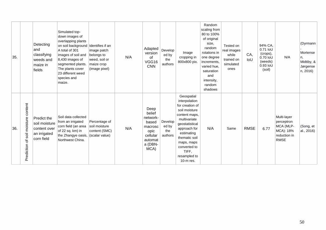
50
35.
Detecting
and
classifying
weeds and
maize in
fields
Simulated top-
down images of
overlapping plants
on soil background
A total of 301
images of soil and
8,430 images of
segmented plants.
The plants cover
23 different weed
species and
maize.
Identifies if an
image patch
belongs to
weed, soil or
maize crop
(image pixel)
N/A
Adapted version
of VGG16
CNN
Develop
ed by
the
authors
Image
cropping in
800x800 pix.
Random
scaling from
80 to 100%
of original
size,
random
rotations in
one degree
increments,
varied hue,
saturation
and
intensity,
random
shadows
Tested on
real images
while
trained on
simulated
ones
CA,
IoU
94% CA, 0.71 IoU (crops), 0.70 IoU (weeds) 0.93 IoU
(soil)
N/A
(Dyrmann
,
Mortense
n,
Midtiby, &
Jørgense
n, 2016)
36.
Pre
dic
tio
n o
f so
il m
ois
ture
conte
nt
Predict the
soil moisture
content over
an irrigated
corn field
Soil data collected
from an irrigated
corn field (an area
of 22 sq. km) in
the Zhangye oasis,
Northwest China.
Percentage of
soil moisture
content (SMC)
(scalar value)
N/A
Deep belief
network-based
macroscopic
cellular automata (DBN-MCA)
Develop
ed by
the
authors
Geospatial
interpolation
for creation of
soil moisture
content maps,
multivariate
geostatistical
approach for
estimating
thematic soil
maps, maps
converted to
TIFF,
resampled to
10-m res.
N/A Same RMSE 6.77
Multi-layer
perceptron
MCA (MLP-
MCA): 18%
reduction in
RMSE
(Song, et
al., 2016)

51
37.
Anim
al re
searc
h
Practical and
accurate
cattle
identification
from 5
different
races
1,300 images
collected by the
authors.
5 classes:
Cattle races,
Bali
Onggole or
Pasuruan,
Aceh
Madura and
Pesisir
N/A GLCM –
CNN
Deep
Learning
Matlab
Toolbox
GLCM
features
extraction
(contrast,
energy and
homogeneity),
saliency maps
to accelerate
feature
extraction
N/A Same CA 93.76%
CNN without
extra inputs:
89.68%
Gaussian
Mixture
Model
(GMM): 90%
(Santoni,
Sensuse,
Arymurth
y, &
Fanany,
2015)
38.
Predict
growth of
pigs
160 pigs, housed
in two climate
controlled rooms,
four pens/room, 10
pigs/pen.
Ammonia, ambient
and indoor air
temperature and
humidity, feed
dosage and
ventilation
measured at 6-
minute intervals.
Estimation of
the weight of
pigs (scalar
value)
N/A First-order DRNN
Develop
ed by
the
authors
N/A N/A
Tested on
different
rooms of
pigs than
the ones
which were
used for
training
MSE,
MRE
0.002
(MSE) on
same
dataset),
10%
(MRE) in
relation to
a
controller
N/A
(Demmer
s T. G.,
Cao,
Parsons,
Gauss, &
Wathes,
2012)
39.
Control of
the growth of
broiler
chickens
Collecting data
from 8 rooms,
each room
housing 262
broilers,
measuring bird
weight, feed
amount, light
intensity and
relative humidity.
Estimation of
the weight of
chicken (scalar
value)
N/A First-order DRNN
Develop
ed by
the
authors
N/A N/A
Tested on
different
rooms of
chicken
than the
ones which
were used
for training
MSE,
MRE
0.02
(MSE),
1.8%
(MRE) in
relation to
a
controller
N/A
(Demmer
s T. G., et
al., 2010)
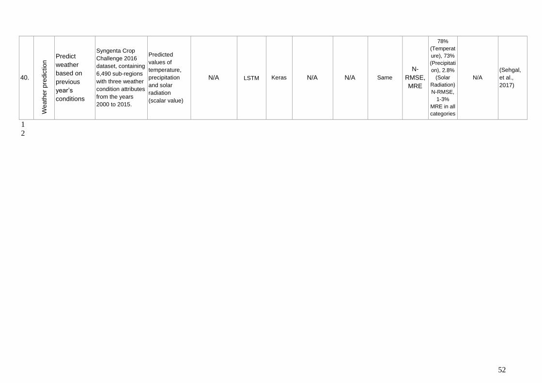
52
40.
Wea
ther
pre
dic
tion
Predict
weather
based on
previous
year’s
conditions
Syngenta Crop
Challenge 2016
dataset, containing
6,490 sub-regions
with three weather
condition attributes
from the years
2000 to 2015.
Predicted
values of
temperature,
precipitation
and solar
radiation
(scalar value)
N/A LSTM Keras N/A N/A Same
N-
RMSE,
MRE
78%
(Temperat
ure), 73%
(Precipitati
on), 2.8%
(Solar
Radiation)
N-RMSE,
1-3%
MRE in all
categories
N/A
(Sehgal,
et al.,
2017)
1
2

53
Appendix III: Publicly-available datasets related to agriculture.
No. Organization/Dataset Description of dataset Source
1. Image-Net Dataset Images of various plants (trees, vegetables, flowers) http://image-net.org/explore?wnid=n07707451
2. ImageNet Large Scale Visual
Recognition Challenge (ILSVRC) Images that allow object localization and detection
http://image-net.org/challenges/LSVRC/2017/#det
3. University of Arcansas, Plants
Dataset Herbicide injury image database
https://plants.uaex.edu/herbicide/
http://www.uaex.edu/yard-garden/resource-library/diseases/
4. EPFL, Plant Village Dataset Images of various crops and their diseases https://www.plantvillage.org/en/crops
5. Leafsnap Dataset Leaves from 185 tree species from the Northeastern
United States.
http://leafsnap.com/dataset/
6. LifeCLEF Dataset Identity, geographic distribution and uses of plants http://www.imageclef.org/2014/lifeclef/plant
7. PASCAL Visual Object Classes
Dataset
Images of various animals (birds, cats, cows, dogs,
horses, sheep etc.)
http://host.robots.ox.ac.uk/pascal/VOC/
8. Africa Soil Information Service
(AFSIS) dataset Continent-wide digital soil maps for sub-Saharan Africa
http://africasoils.net/services/data/
9. UC Merced Land Use Dataset A 21 class land use image dataset http://vision.ucmerced.edu/datasets/landuse.html
10. MalayaKew Dataset Scan-like images of leaves from 44 species classes. http://web.fsktm.um.edu.my/~cschan/downloads_MKLeaf_d
ataset.html
11. Crop/Weed Field Image Dataset Field images, vegetation segmentation masks and
crop/weed plant type annotations.
https://github.com/cwfid/dataset
https://pdfs.semanticscholar.org/58a0/9b1351ddb447e6abd
ede7233a4794d538155.pdf
12. University of Bonn
Photogrammetry, IGG
Sugar beets dataset for plant classification as well as
localization and mapping.
http://www.ipb.uni-bonn.de/data/
13. Flavia leaf dataset Leaf images of 32 plants. http://flavia.sourceforge.net/
14. Syngenta Crop Challenge 2017
2,267 of corn hybrids in 2,122 of locations between
2008 and 2016, together with weather and soil
conditions
https://www.ideaconnection.com/syngenta-crop-
challenge/challenge.php
1