deep learning for early detection, identification, and
TRANSCRIPT
Claremont Colleges Claremont Colleges
Scholarship @ Claremont Scholarship @ Claremont
CGU Theses & Dissertations CGU Student Scholarship
Spring 2021
Deep Learning for Early Detection, Identification, and Deep Learning for Early Detection, Identification, and
Spatiotemporal Monitoring of Plant Diseases Using Multispectral Spatiotemporal Monitoring of Plant Diseases Using Multispectral
Aerial Imagery Aerial Imagery
Joseph Kimani Mbugua Claremont Graduate University
Follow this and additional works at: https://scholarship.claremont.edu/cgu_etd
Recommended Citation Recommended Citation Mbugua, Joseph Kimani. (2021). Deep Learning for Early Detection, Identification, and Spatiotemporal Monitoring of Plant Diseases Using Multispectral Aerial Imagery. CGU Theses & Dissertations, 218. https://scholarship.claremont.edu/cgu_etd/218. doi: 10.5642/cguetd/218
This Open Access Dissertation is brought to you for free and open access by the CGU Student Scholarship at Scholarship @ Claremont. It has been accepted for inclusion in CGU Theses & Dissertations by an authorized administrator of Scholarship @ Claremont. For more information, please contact [email protected].

Deep Learning for Early Detection, Identification,
and Spatiotemporal Monitoring of Plant Diseases
Using Multispectral Aerial Imagery
By
Joseph Kimani Mbugua
Claremont Graduate University
2021

©Copyright Joseph Kimani Mbugua, 2021.
All rights reserved

APPPROVAL OF THE REVIEW COMMITTEE
This dissertation has been duly read, reviewed, and critiqued by the Committee listed
below, which hereby approves the manuscript of Joseph Kimani Mbugua as fulfilling the
scope and quality requirements for meriting the degree of Doctor of Philosophy in
Information Systems & Technology.
Dr. Brian Hilton, Chair
Claremont Graduate University
Clinical Full Professor of GIS
Dr. Lorne Olfman, Member
Claremont Graduate University
Professor and Director
Dr. Zachary Dodds, Member
Harvey Mudd College
Professor of Computer Science

Abstract
Deep Learning for Early Detection, Identification, and Spatiotemporal Monitoring of
Plant Diseases Using Multispectral Aerial Imagery
By
Joseph Kimani Mbugua
Claremont Graduate University: 2021
Production of food crops is hampered by the proliferation of crop diseases which cause
huge harvest losses. Current crop-health monitoring programs involve the deployment
of scouts and experts to detect and identify crop diseases through visual observation.
These monitoring schemes are expensive and too slow to offer timely remedial
recommendations for preventing the spread of these crop-damaging diseases. There is
thus a need for the development of cheaper and faster methods for identifying and
monitoring crop diseases.
Recent advances in deep learning have enabled the development of automatic and
accurate image classification systems. These advances coupled with the widespread
availability of multispectral aerial imagery provide a cost-effective method for
developing crop-diseases classification tools. However, large datasets are required to
train deep learning models, which may be costly and difficult to obtain. Fortunately,
models trained on one task can be repurposed for different tasks (with limited data)
using transfer learning technique. The purpose of this research was to develop and

implement an end-to-end deep learning framework for early detection and continuous
monitoring of crop diseases using transfer learning and high resolution, multispectral
aerial imagery.
In the first study, the technique was used to compare the performance of five pre-
trained deep learning convolutional neural networks (VGG16, VGG19, ResNet50,
Inception V3, and Xception) in classifying crop diseases for apples, grapes, and
tomatoes. The results of the study show that the best performing crop-disease
classification models were those trained on the VGG16 network, while those trained on
the ResNet50 network had the worst performance.
The other studies compared the performance of using transfer learning and different
three-band color combinations to train single- and multiple-crop classification models.
The results of these studies show that models combining red, near infrared, and blue
bands performed better than models trained with the traditional visible spectral band
combination of red, green, and blue. The worst performing models were those
combining near infrared, green, and blue bands.
This research recommends that further studies be undertaken to determine the best
band combinations for training single- and multi-label classification models for both
crops and plants and diseases that affect them.
DEDICATION
This dissertation is dedicated to my wife:
Hellen Wanjiku Kimani
And my children:
Jeivis Wanjiku Kimani
&
Jeremy Mbugwa Kimani
Yes, I know I have been ‘away’ for too long.
Thank you for your sacrifice, support, and understanding.
All Together Now!!
Baba is finally back!

vii
ACKNOWLEGDEMENTS
I would like to first offer my unreserved and special thanks to the members of my
dissertation committee. Thank you, Dr. Brian Hilton, for chairing the committee and
providing reading materials, professional and technical support, guidance, and feedback
throughout the dissertation period. Thank you, Dr. Lorne Olfman, for providing insights
and for your detailed reviews of my draft manuscripts. And thank you, Dr Zach Dodds,
for your support on Python programming language and for offering detailed insights
and guidance on the nuances of computer vision.
I would like to thank Pamela M. Mullin for awarding me the Dream and Believe Award
in 2018. Echoing the words of Jonas Salk that you quoted on the award certificate, I
sincerely thank you for helping make my dreams into reality.
I would also like to thank the following institutions for their support which enabled me
to finance and complete this research on a timely basis: The Microsoft Corporation for
awarding me the AI for Earth Sponsorship that provided tools and GPU compute time
on the company’s Azure cloud computing platform. Special thanks also to ESRI for
offering me the spatial processing software on the Microsoft’s Azure platform for free.
Finally, thanks to Claremont Graduate University for granting me the 2018 dissertation
award. Your awards are highly appreciated for relieving my financial burdens.

viii
Table of Contents
Table of Figures ............................................................................................ xi
List of Tables .............................................................................................. xiv
List of Abbreviations ................................................................................... xv
Chapter 1: Introduction .............................................................. 1
Chapter 2: Literature Review ...................................................... 7
2.1 Low-Level Image Descriptors ................................................................................. 13
2.2 Neural Networks ..................................................................................................... 14
2.3 Deep Learning ......................................................................................................... 15
2.4 Convolutional Neural Networks (CNNs) ................................................................. 17
2.4.1 CNN Layers ...................................................................................................... 18
2.4.2 ImageNet ......................................................................................................... 20
2.4.3 CNN Performance ........................................................................................... 20
2.5 Transfer Learning.................................................................................................... 22
Chapter 3: Methodology ............................................................ 27
3.1 Proposed Framework for Crop Disease Monitoring ............................................... 27
3.1.1 Spectral Behavior of Leaves and Canopies ...................................................... 28

ix
3.1.2 Early Disease Detection ................................................................................... 29
3.2 Transfer Learning Using the Keras Python Library ............................................... 35
3.3 Model Selection ....................................................................................................... 35
3.3.1 VGG16 and VGG19 ........................................................................................... 36
3.3.2 Inception V3 ................................................................................................... 37
3.3.3 ResNet50 ......................................................................................................... 38
3.3.4 Xception ........................................................................................................... 39
3.3.5 Summary of Model Selection .......................................................................... 40
3.4 Transfer Learning Workflow in Azure .................................................................... 41
3.5 Comparing the Performance of Pre-Trained Deep Learning Models in Classifying
Crop Diseases........................................................................................................... 41
3.5.1 The Fine-Tuning Process ................................................................................. 45
3.6 Comparing the Performance of Crop Classification Models Trained on Different
Three-Band Combination Images ........................................................................... 50
3.6.1 Cropland Data Layer (CDL) ............................................................................. 51
3.6.2 National Agriculture Imagery Program (NAIP) Imagery ............................... 53
3.6.3 Procedure for Extracting Training Data for Each Crop .................................. 53
3.6.4 Training Single and Multi-Crop Classification Models .................................. 56
3.7 Using the Best-Performing Multi-Crop Classification Model to Classify NAIP
Imagery .................................................................................................................... 60
3.8 Data Analysis ........................................................................................................... 63
x
3.9 Summary ................................................................................................................. 64
Chapter 4: Data Analysis and Results ........................................ 66
4.1 Comparing the Performance of Pre-Trained Deep Learning Networks ................. 70
4.2 Comparing the Performance of Different Band Combination Crop Classification
Models...................................................................................................................... 78
4.2.1 Using Three-Band Combination Models to Classify Single Crops ................. 78
4.2.2 Using Three-Band Combination Models to Classify Three Crops ................. 80
4.2.3 Using Three-Band Combination Models to Classify Four Crops ................... 83
4.4 Making Inferences from Unseen NAIP Imagery .................................................... 84
4.5 Summary ................................................................................................................. 85
Chapter 5: Discussion and Conclusions .................................... 87
5.1 Conclusions .............................................................................................................. 94
5.1.1 Crop Disease Classification .............................................................................. 94
5.1.2 Band Combination Classification Models ....................................................... 95
5.2 Significance of Research Findings .......................................................................... 96
5.3 Limitations of Research .......................................................................................... 97
5.4 Recommendations for Future Research ................................................................. 98
Appendix ................................................................................. 107

xi
Table of Figures
Figure 2.1: Classic Machine Learning Classification for Cassava Mosaic Disease (CMD)
........................................................................................................................................... 14
Figure 2.2: A simple Neural Network with One Hidden Layer ........................................ 15
Figure 2.3: Learning Differences Between Classic and Deep Learning Methods ............ 16
Fig 2.4: AlexNet Convolutional Neural Network Architecture......................................... 19
Figure 2.5: Recent Improvements in ImageNet ............................................................... 21
Classification Accuracy Using Deep Learning Models ..................................................... 21
Figure 2.6: Differences in Learning Processes ................................................................. 24
Between Traditional Machine Learning and Transfer Learning ...................................... 24
Figure 2.7: Transfer Learning Data Size-Similarity Matrix and Decision Map ............... 26
Figure 3.1: Spectral Reflectance from a Living Leaf ......................................................... 29
Figure 3.2: Early Disease Detection: Collect Pre-Disease Training Data Task ................ 31
Figure 3.3: Framework for Early Detection and Continuous Monitoring of Crop Diseases
........................................................................................................................................... 32
Figure 3.4: Visualization of VGG Architecture ................................................................. 37
Figure 3.5: Original Inception Module as used in GoogleNet .......................................... 38
Figure 3.6: Residual Learning Building Block .................................................................. 39
Figure 3.7: The Xception Architecture. ............................................................................. 40
Figure 3.8: Transfer Learning Workflow in Azure ........................................................... 41
Figure 3.10: Fine-Tuning a Pre-Trained VGG16 Network ............................................... 49
Figure 3.11: California Cropland Data Layers (CDLs) Areas of Interest (AOI) ................ 52
Figure 3.12: Four-Band NAIP Mosaic for Grapes AOI ..................................................... 55

xii
Figure 3.13: Extracting Grapes Training Samples from Four 3-Band Raster Layers ...... 56
Figure 3.14: Extracted Training Data for the Three Crops RGB Classification Model .... 60
Figure 3.15: Map of Areas of Interest (AOIs) for Separate and Combined Crops ........... 62
Figure 3.16: All 3 Crops AOI CDL layers over the NAIP Mosaic Layer ........................... 62
Figure 4.1: Screenshot Jupyter Notebook Python Code for Splitting Datasets ............... 68
Figure 4.2: Screenshot Jupyter Notebook Python Code for Data Augmentation and ..... 69
Model Training .................................................................................................................. 69
Figure 4.3: Training and Validation Accuracies and Losses for VGG16 Models ............. 72
Figure 4.4: Training and Validation Accuracies and Losses for ResNet50 Models ......... 73
Figure 4.5: Training and Validation Accuracies and Losses for VGG19 Models ............. 73
Figure 4.6: Training and Validation Accuracies and Losses for Inception Models ......... 74
Figure 4.7: Training and Validation Accuracies and Losses for Xception Models .......... 74
Figure 4.8: Confusion Matrices for VGG16 Single Crop Disease Classification Models . 75
Figure 4.9: Confusion Matrix for VGG16 All Crops Disease Classification Model .......... 76
Figure 4. 10: VGG16 Model Predictions............................................................................ 77
Figure 4.11: Confusion Matrices for Single Crop Classification Models .......................... 80
Using Different Band Combinations ................................................................................. 80
Figure 4.12: Confusion Matrices for Three Crops Classification Models ......................... 82
Figure 4.13: Confusion Matrices for Four Crops Classification Models .......................... 84
Figure 4.14: RGB Three Crops Model Predictions ........................................................... 85
Figure 5.1: Visual Similarities of Early and Late Blight Tomato Diseases ....................... 91
Figure A1: Confusion Matrices for VGG19 Single Crop Disease Classification Models . 107
Figure A2: Confusion Matrix for VGG19 All Crops Disease Classification Model ......... 108

xiii
Figure A3: Confusion Matrices for ResNet50 Single Crop Disease Classification Models
......................................................................................................................................... 108
Figure A4: Confusion Matrix for ResNet50 All Crops Disease Classification Model .... 109
Figure A5: Confusion Matrices for Inception Single Crop Disease Classification Models
......................................................................................................................................... 109
Figure A6: Confusion Matrix for Inception All Crops Disease Classification Model ...... 110
Figure A8: Confusion Matrix for Xception All Crops Disease Classification Model ...... 112
xiv
List of Tables
Table 3.1: Crop Health/Disease Classes Labels and Training Data Summary ................ 44
Table 3.2: Fine-Tuned Layers, Type and Number of Fine-Tuned Parameters for each
Pre-Trained Network ........................................................................................................ 47
Table 3.3: Three-Band Combinations Classes Training Data Summary ......................... 58
Table 4.1: Models Training Results .................................................................................... 71
Table 4.2: Training Results for Three-Band Combination Single Crop Models .............. 79
Table: 4.3: Training Results for Three-Band Combination Three Crops Models ............ 81
Table: 4.4: Training Results for Three-Band Combination Four Crops Models ............. 83
Table 5.1: Fine-Tuned Parameters as a Percentage of Total Parameters ......................... 90
xv
List of Abbreviations
ANN Artificial Neural Network
AOI Area of Interest
BLS Brown Leaf Spot
CBSD Cassava Brown Streak Disease
CDL Cropland Data Layer
CMD Cassava Mosaic Disease
CNN Convolutional Neural Network
ConvNet Convolutional Neural Network
DCNN Deep Convolutional Neural Network
GeoAI VM Geo Artificial Intelligence Virtual Machine
HOG Histogram of Oriented Gradients
ILSVRC ImageNet Large Scale Visual Recognition Challenge
KNN K-Nearest Neighbor
NAIP National Agriculture Imagery Program
NDVI Normalized Difference Vegetation Index
ReLU Rectified Linear Unit
RGB Red, Green, and Blue
RGBI Red, Green, Blue, and Near Infrared
SIFT Scale Invariant Feature Transform
SURF Speed Up Robust Feature
SVM Support Vector Machine
UAVs Unmanned Aerial Vehicles

xvi
USDA United States Department of Agriculture
1
Chapter 1: Introduction
Various types of crop, plant, and fruit diseases can significantly reduce the quality and
yield of produce. According to a report by Food and Agriculture organization of the
United Nations (F.A.O, 2019b), plants are crucial contributors to global food security
and constitute 80% of the human diet. The essential contribution of plants to food
security is however threatened by plant pests and diseases which damage crops and
cause food shortages by, thereby reducing the amounts of food available and access to
food. The damages caused by plant pests and diseases thus lead to increased food costs
and they may also affect the palatability of the food. The report also notes that plant
pests and diseases cause losses of 20 to 40% of the food produced worldwide with an
estimated value of more than $ 220 billion. In sub-Saharan Africa, for example, cassava
mosaic disease (CMD) and cassava brown streak disease (CBSD) are viral diseases
responsible for cassava losses of more than 1 billion US dollars annually (Ramcharan et
al., 2017).
To detect and monitor plant health and other field conditions, developed countries
employ expensive and time-consuming ground surveys and monitoring programs (Xiao
& Mcpherson, 2005). For example, the detection and monitoring component of the US
forest health monitoring program, which collects data on the prevailing conditions of
the forest ecosystem, is conducted annually (Alexander & Palmer, 1999). The
evaluation-monitoring component of the program is only activated if a problem or
abnormality is observed after analyzing the detection monitoring data. This phase of
monitoring involves the evaluation of the extent, severity, and probable causes of any of
2
the health abnormality observed. Such a monitoring program takes too long to identify
the forest condition and may result in misplaced and costly application of remedial
actions since the conditions are detected at very low spatial and temporal resolutions.
Furthermore, this scouting approach and the use of experts to detect and identify plant
diseases by visual observation is slow, expensive, and labor-intensive (Dubey & Jalal,
2014). Moreover, poor countries lack the means and technical capacities to implement
such monitoring programs.
To meet the food requirements of the world’s increasing population, which the F.A.O
estimates will be about 9.1 billion people by the year 2050 (F.A.O, 2019a), there is a
need to increase food production by more than 70% of the current levels. To fulfil this
increasing need, the agricultural industry uses chemicals such as bactericides,
fungicides, and nematicides to control plant pests and diseases. The use of these
chemicals causes adverse effect on the agro-ecosystem and the environment. To control
and manage the spread of crop diseases and avert the food security crisis they portend,
particularly in sub-Saharan Africa, there is thus a need to develop new environmental-
friendly methods for early detection and identification of the diseases.
The proliferation of unmanned aerial vehicles (UAVs), public, and private satellites, has
enabled the imaging of almost all locations on earth at high temporal, spectral, and
spatial resolutions at relatively low cost. The availability of high-resolution multispectral
aerial imagery provides an opportunity for the continuous monitoring of crop diseases
and plant health globally at a relatively lower cost than would be incurred by deploying
the more expensive traditional methods.

3
The development of novel tools for early detection, identification, and mapping of crop
diseases will reduce the cost, damage, and time taken to monitor and control the
diseases. Early detection of crop diseases improves productivity by enabling the early
application of measures that prevent the spreading of the diseases. This is more effective
than applying curative treatments because diseased plants may develop disease
symptoms when it is too late for the such treatments to be effective (Fahrentrapp et al.,
2019). Besides improving productivity, the tools will also enable the deployment of
efficient management practices to control the diseases. Moreover, early detection of the
diseases will eliminate the need to use excessive amounts of pesticides and chemicals to
manage them, thus ensuring that the dangers of contaminating ground water and
accumulating toxic residues in agricultural products due to excessive usage of pesticides
and chemicals can be avoided (Dubey & Jalal, 2014; Mohanty et al., 2016).
Whereas object detection and identification methods have been developed to detect and
identify objects in traditional images, no documented methods for the automatic
detection, identification, and mapping of crop diseases using high resolution
multispectral aerial images of crop fields have been developed so far in sub-Saharan
Africa. This research uses the deep learning approach to develop and implement a
framework for the near-real time ingestion of multispectral aerial and satellite imagery
to detect, identify, monitor, and map crop diseases in agricultural fields at regional
levels.
The main purpose of this research was to contribute to the understanding of how
multispectral aerial imagery can be used to build deep learning models for early

4
detection and identification of crop diseases before their symptoms become visible to
the naked eye. The specific objectives of this study were:
1. To develop a deep learning framework for early detection and continuous
monitoring of crop diseases.
2. To investigate the viability of using pre-trained deep learning networks to train
crop disease classification models and evaluate the trained models’ performance to
determine the best-suited network for training such models.
3. To evaluate the combination of spectral bands (natural and false-color composites)
that are best suited for training classification models for detecting and identifying
different crops jointly and severally.
Deep learning models require the use of large datasets of imagery during training to
ensure that the model developed can generalize to unseen data. One of the main data
challenges experienced in undertaking this research was the unavailability of adequate
labelled aerial imagery to train the deep learning models. To address this challenge, data
augmentation techniques, which are analogous to synthetic generation of more data
from the available training data, were used. Another technique that was used to address
this problem was the implementation of transfer learning (Karpathy, 2017), where pre-
trained deep learning models were repurposed and used to train classification models
for the studies undertaken in this research.
Current research on the use of machine learning and imagery to monitor crop health has
mostly relied on the use of leaf images of crops captured using smartphones and hand-
held digital cameras (Aduwo et al., 2010; Hughes & Salathé, 2015; Mwebaze &
5
Owomugisha, 2016). No known or published research has used whole crop canopy aerial
imagery to detect and identify crop diseases in sub-Saharan Africa. While the use of leaf
images is appropriate for the use case where farmers capture images of the diseased
leaves and pass them to a phone application to diagnose the disease, the use of whole
canopy images, which are investigated this research, will enable the development of an
automated and smart-device accessible diagnosis monitoring system for large land areas
that ingests new aerial images and processes them to detect, identify, and map crops
and crop diseases at their early stages.
Whereas the original idea of this research was to use whole canopy aerial images of
healthy and diseased cassava images, this research was unable to acquire high
resolution whole canopy cassava images during the duration of the study. Thus, leaf
images of apples, corn, grapes, and tomatoes were used instead to demonstrate how the
workflow proposed in the developed framework could be implemented. However, for
future implementation of the developed framework, this study suggests that whole
canopy crop images be used instead of leaf images.
This research is significant because it has developed a new algorithm for the early
detection of crop diseases using high resolution multispectral imagery. Previous
research on crop disease detection has concentrated on the use of imagery captured in
the visible spectrum. Thus, the machine learning models developed so far can only be
applied to identify diseases whose symptoms are already visible to the naked eye in the
red, green, and blue (RGB) visible bands of the spectrum. Although only crop diseases
images captured in RGB bands were used in this study, it is proposed that the developed
framework be implemented using composite images derived from different band

6
combinations from all the available bands in the multispectral aerial imagery. One of the
original goals of this research was to investigate whether a deep learning neural network
model could be trained to detect and identify crops and crop diseases before they
became visible to the naked eye by using composite imagery of bands in the visible and
the invisible parts of the spectrum. However, this novel technique was only used to
develop crop classification models in this research due to the unavailability of
multispectral crop diseases imagery that incorporate bands in the invisible parts of the
spectrum. In this regard, this research is also significant because the early disease
detection and monitoring method it has developed will facilitate the mapping of crop
diseases before they can be visually observed, hence enabling the deployment of efficient
and environment-friendly crop disease management practices.
The remainder of this dissertation is organized as follows. Chapter 2 presents a
literature review of the advances made in the use of machine learning methods to
monitor crop diseases and their limitations; Chapter 3 details the transfer learning
methodology, deep learning model selection, data acquisition and processing, and the
proposed data analysis methods; Chapter 4 presents the findings of the various studies
undertaken in this research; and Chapter 5 offers detailed discussions, conclusions,
limitations, applications of the research findings, and suggestions for future research.

7
Chapter 2: Literature Review
To diagnose cassava diseases, crop disease experts visit cassava fields and identify the
diseases by visually observing the leaves for symptoms of the diseases (Mwebaze &
Owomugisha, 2016). In forest health monitoring, for example, the USDA Forest Service
conducts an annual aerial survey using aerial observers who sketch maps of their
observation showing the estimated number and species or genus of damaged trees, and
the types of damages observed (United States Department of Agriculture, 2017). This
method of visual identification of plant diseases is subjective and unreliable given that
even experts do not always agree on their diagnoses. Moreover, the method is slow and
is highly dependent on the availability of trained experts who may not be available in
many developing countries.
Although advances in machine learning have led to an increase in the automation of
expert tasks in various domains, the application of machine learning in agriculture for
monitoring crop and plant health is fledgling compared to other domains where the
technique is widely applied for various computer vision tasks. Despite the limited
application in agriculture, some research has nevertheless been undertaken to identify
and classify diseases in cassava and other crops. Most of the research undertaken in this
area has, however, treated the issue of crop disease detection as a binary classification
problem, where low-level image features are hand-extracted and used to differentiate
between healthy and diseased crops. Most of these studies have also used small samples
of leaf images of healthy and diseased crops and plants that were captured mainly in
controlled background and lighting conditions. Research on disease detection and
8
identification in cassava and other crops is mainly based on automated image
recognition through low-level image feature extraction, whereas machine learning
methods have demonstrated promising results as shown in the studies highlighted
below.
In a study aimed at detecting and identifying crop diseases, Aduwo et al. (2010) used
standard classification methods and low-level image features (color and shape)
extracted from cassava leaf images in Uganda to develop an automated and accurate
method for diagnosing Cassava Mosaic Disease (CMD) on cluttered images captured in
the field using a standard digital camera.
In a similar study, Mwebaze and Owomugisha (2016) used cassava leaf images captured
in situ in Uganda using smartphones to develop a smartphone-based diagnostic system
for detecting and classifying four cassava diseases and five severity levels of the diseases
(healthy to severely diseased plants). This study, unlike most of the other studies
discussed here, used a large dataset of images (>7K images) that were captured with a
smartphone in the field. The application enables farmers to capture cassava leaf images
with their smartphones and upload them to a back-end remote server. A score
indicating the disease and the severity level of the uploaded image is then returned to
the farmer immediately. Their study showed that using different feature extraction
methods affected the accuracy of the classifier.
Researchers have also conducted studies to detect and identify diseases in other crops.
For example, Gibson et al. (2015) developed an automated and scalable classifier system
for detecting major wheat diseases in noisy and cluttered field imagery. The system uses
a high-dimensional texture image descriptor together with a randomized forest
9
approach for primary leaf recognition. Tests of the system using a dataset of standard
smartphone-captured field imagery of wheat leaves showed that it could accurately
detect and identify the type of the disease in a leaf image. In another study on wheat,
Siricharoen et al. (2016) developed a lightweight mobile phone system for monitoring
non-diseased leaves and five wheat diseases (brown rust, Septoria, yellow rust, powdery
mildew, and tan spots). The standalone system uses the built-in smartphone capability
to capture and pre-process the image of the main leaf of wheat for quality and
consistency. Nine low-level image feature descriptors based on color, texture, and shape
(including disease shapes) are extracted from the leaf image and used to classify the
image on the mobile system within seconds after capturing the image, with an accuracy
of about 88%.
Other researchers have undertaken studies for monitoring and detection of diseases
using shallow neural networks. In one such study, Abdullakasim et al. (2011) developed
an image analysis technique for automated monitoring and detection of brown leaf spot
(BLS) disease in cassava under field conditions. They trained a binary classifier with a
fully connected, feed-forward Artificial Neural Network (ANN) with an input of 10 color
indices (used as color descriptors) using cassava leaf images that were taken with a
digital camera in Thailand. They evaluated different network architectures of the ANN,
which differed depending on the number neurons in the hidden layer. Using this
technique, the best architectures attained classification accuracies of 79% and 90% for
diseased and healthy plants, respectively. Though the image-analysis technique
developed in this study was deemed to be feasible for in-field detection of visible
10
symptoms of BLS, the researchers suggested that it could be improved further by using
better-illuminated and segmented images.
Similar studies have also been conducted to identify diseases in fruits. In one study,
Dubey and Jalal (2014) developed and evaluated a machine learning framework that
uses images to identify fruit diseases. In this method, images of the diseased fruits are
first segmented using K-Means clustering followed by extraction of color and texture
features (statistical color and texture descriptors). Finally, a multi-class support vector
machine (SVM) is used to classify the diseases. The researchers evaluated their
approach by applying the framework in the identification of three apple diseases,
namely: apple scab, apple blotch, and apple rot. Their results showed that the
framework could be used to detect and identify the diseases tested with an accuracy of
up to 93%.
The application of machine learning in agriculture can also help farmers employ
precision agriculture production systems, which enable the application of management
practices that vary across a field based on differences in in-field conditions (Seelan et al.,
2003). Such management systems increase the productivity and returns of farms by
enabling farmers to use reduced amounts of resources such as fertilizers, water,
pesticides, etc. and apply them to only those sections of the field where they are needed.
Monitoring of differences in crop vigor within fields can be achieved by using high-
resolution multi-spectral imagery. In wheat fields, for example, Franke and Menz
(2007) investigated the potential of using high-resolution, multi-spectral remote
sensing imagery for a time series analysis of crop diseases aimed at detecting differences
in crop vitality within the fields to enable site-specific application of fungicides based on
11
observed differences. They used three high-resolution remote sensing images to analyze
the spatial-temporal infection dynamics of a wheat plot at various pathogen-infection
stages of two wheat diseases, powdery mildew (Blumeria graminis) and leaf rust
(Puccinia recondita). Using a decision-tree filtering method and the Normalized
Difference Vegetation Index (NDVI), they were able to accurately classify different areas
of the plot based on disease severity.
Unmanned aerial vehicles (UAVs) are increasingly being used as platforms for acquiring
multispectral aerial imagery for monitoring crop health in precision agriculture
production systems. Puig et al. (2015), for example, explored the use of a combination of
unmanned aerial vehicles (UAVs), remote sensing, and machine learning techniques to
monitor, and assess near real-time crop damage caused by agricultural pests. The
monitoring enables the application of optimal in-field site-specific treatments that
reduce crop losses and pest management costs. They used an orthoimage created from
high-resolution RGB images of a sorghum crop that was severely damaged by white
grubs (Coleoptera: Scarabaeidae) collected in Australia using an UAV platform. The
authors used an unsupervised machine learning approach to classify the crop damage
into three crop health levels, namely: bare soil with no plants, transition zones, and
healthy canopy areas. Using Gaussian convolution kernels and K-means clustering, their
study showed that it was possible to consistently classify the sorghum field into the three
clusters of crop health, and to create class-membership maps that could be used to
estimate the area of each crop health level based on the class membership of each
individual pixel.

12
Training a deep learning model to solve problems for a specific domain requires a large
amount of data. When such data is not readily available, alternative approaches, e.g.,
transfer learning, are used to address the problem. Using transfer learning, models
trained on one task can be reused to solve different problems in the same domain or
similar problems in a different domain. For example, Ramcharan et al. (2017) applied
transfer learning to train the GoogleNet Inception v3 deep convolutional neural network
model (Christian Szegedy, Liu, et al., 2015b) to identify three cassava diseases and two
pest damages using a dataset of healthy and diseased cassava leaf images taken in the
field in Tanzania. They also analyzed the performance of three classifiers (SoftMax,
SVM, and KNN) on the transfer learning model in identifying the presence or absence of
the diseases in the images. Their results showed that transfer learning approach could
successfully be used on the pre-trained GoogleNet model (as a featurizer/feature
extractor) to achieve a high classification accuracy of cassava diseases without requiring
a large dataset of cassava-leaf images taken in the field. They also observed that
augmenting the image dataset by cropping the original leaf images into individual
leaflets improved the detection accuracy. Their analysis also showed that the SVM
classifier attained higher accuracies in identifying most of the diseases in the study
compared to the other two classifiers. They concluded that the transfer learning
approach can be successfully deployed as an accurate, fast, and affordable digital system
for the in-field detection of plant diseases.
Deep learning has also been used to identify crops and for crop health monitoring.
Mohanty et al. (2016) trained a deep convolution neural network to identify 14 different
crops species and 26 diseases or their absence using a public dataset of images from
13
PlantVillage (Hughes & Salathé, 2015) of diseased and healthy plant leaves that were
taken under controlled conditions. They used the AlexNet (Krizhevsky et al., 2012) and
GoogleNet(Christian Szegedy, Liu, et al., 2015a) deep convolutional neural networks
models and the open-source Caffe deep learning framework (Jia et al., 2014) to train
their model in two ways: using the two models’ architecture to train their model from
scratch, and by using the transfer learning approach of reusing already pre-trained
models of the two networks that had been trained on the ImageNet Large Scale Visual
Recognition Challenge (ILSVRC) dataset (Deng et al., 2009). Their best model was able
to correctly identify crop-disease pairs with an accuracy of 99%. However, the models
performed poorly on images captured under conditions that were different from the
ones in the PlantVillage dataset, implying that the training dataset may have overfitted
the model. According to the researchers, one of the main limitations of practical
application of their model was the use of up-facing single-leaf images captured on a
homogeneous background to train the model instead of using images of the diseases as
they naturally appear on plants.
Some of these limitations were addressed in this research by, for example, training crop
classification models using aerial imagery that captured the whole crop canopies as they
naturally appear rather than capturing isolated images of single leaves.
2.1 Low-Level Image Descriptors
Hand-engineered features extracted from images have traditionally been used with
machine learning approaches for computer vision tasks such as image classification and
detection of plant diseases. The hand-engineered image features are extracted using
methods such as SURF (Bay et al., 2008), SIFT (Lowe, 2004), and HOG (Dalal &

14
Triggs, 2005; Schmidhuber, 2015). Examples of other image processing techniques used
to detect, quantify severity of, and classify plant diseases are documented in a survey by
Barbedo (2013). The hand-engineered process of feature extraction and image
enhancement is complex, computationally expensive, time-consuming, difficult to
optimize, and requires domain expert knowledge to engineer the best image features
that differentiate one image class from another. The process also needs to be repeated
each time there is a considerable change in the problem or the dataset being addressed
(Mohanty et al., 2016). Furthermore, the quality of the results obtained through this
approach varies depending on which predefined features are extracted. An example of
the workflow of this classic approach is shown in Figure 2.1.
Figure 2.1: Classic Machine Learning Classification for Cassava Mosaic Disease (CMD)
(adapted from Goodfellow et al. 2016)
2.2 Neural Networks
Artificial neural networks (ANN) are inspired by the human brain which comprises a
network of interconnected neurons. Simple neural networks typically consist of an input

15
layer, one or two hidden layers, and one output layer of neurons. For example, the ANN
used by (Abdullakasim et al., 2011) to recognize brown leaf spot in cassava has only one
hidden layer with a variable number of neurons. In this type of a neural network, every
node in one layer is connected to every node in the next layer as shown in Figure 2.2.
Figure 2.2: A simple Neural Network with One Hidden Layer
Models trained on these simple networks usually have only a few layers because
increasing the number of layers in such a network increases the number of weights that
must be learned, making it arduous to train the network. This led to the development of
deep learning.
2.3 Deep Learning
Advances in machine learning witnessed in recent years can be mainly attributed to the
use of an approach known as deep learning. Deep learning is a field of machine learning

16
that transforms the representation of the input data by leveraging the learning obtained
from sequential layers of increasingly meaningful representation of the data (F Chollet,
2017). A deep learning network is a type of an artificial neural network composed of an
input layer, output layer, and many hidden layers of neurons. Thus, deep learning
derives its name from the sequential layering of data representation and not the depth
of understanding. The increase in computational power of hardware achieved in recent
years, combined with the availability of large datasets and the use of robust training
algorithms, have made it possible to train deep neural networks that outperform the
earlier networks by orders of magnitude. The deep learning approach has been very
successful recently, especially in image classification, speech recognition, and natural
language processing tasks.
Unlike the traditional approach of manual feature extraction, deep learning approaches
do not need to be provided with hand-engineered features since they are able to learn
the features from the large datasets provided during model training. The general
differences in learning between the two systems are shown in Figure 2.3.
Figure 2.3: Learning Differences Between Classic and Deep Learning Methods
(Adapted from Goodfellow et al., 2016)

17
Deep learning has particularly been successful in solving computer vision tasks using a
type of deep learning network called convolutional neural networks (ConvNet or CNN),
which are described in detail in the following section.
2.4 Convolutional Neural Networks (CNNs)
Just like ordinary neural networks, convolutional neural networks (CNNs) consist of
neurons with learnable weights and biases (Karpathy, 2017). Like other neural
networks, CNNs receive an input of raw data (e.g., image pixels in an image
classification task) and give an output of class scores at the end of the network. In
convolutional neural networks, however, each layer has several filters where nodes in
one layer are only connected to a few nodes in a small region of the next layer. The
reduction of the number of connections makes it possible to train deeper networks, with
each layer learning hierarchical concepts of the input data while maintaining the spatial
cohesion of the input (Collins et al., 2017). Additionally, unlike ordinary neural
networks, CNNs assume that the spatial aspect of the input data, such as an image, is
important (Karpathy, 2017). Each filter detects different features or parts of features (of
the image) in the first layers of the CNN, but these features are usually combined in the
deeper layers of the network. A convolution is defined as the element by element
multiplication of the filter and the input image at each image position, while the output
of the convolution is known as a feature map.

18
2.4.1 CNN Layers
A CNN is made of different types of the layers, which are usually stacked together to
form a full CNN architecture. The layers in a generic CNN are stacked such that the
input layer is followed by a series of one or more convolutional layers which are followed
by a pooling layer. The final pooling layer is connected to one or more fully connected
layers, which are finally connected to a classifier, such as Softmax (Rosebrock, 2017) ,
which classifies the input image into the categories on which the network is trained, and
outputs the probabilities for each category. The types of CNN layers are described
below:
1. Input layer: This network entry layer contains the input image which can be
represented by the raw pixel values of the image.
2. Convolutional layer: This layer consists of a set of spatially small learnable filters
that extend through the depth (channels/bands) of the input volume. During the
forward pass of the training process, each filter is moved as a sliding window
across the width and height of the input image and the dot products of the filter’s
values and the values of the small region of the input they are connected to
(convolved) at every position are computed. The output of sliding each filter
across the width and height of the input each image is a 2-dimensional feature
map that represents the response of each filter at every spatial position. The
convolutional layer has the following parameters:
• Number of filters (depth) – Each filter learns to look for a different feature
in the input
• Kernel (filter) size –This controls the pixel dimensions of the filter

19
• Stride – This is the number of pixels the filter is moved during each slide
• Padding – This determines the size of padding (with zeros) that is added
around the borders of the input image to control the spatial size of the
output from the layers.
3. Activation layer: The activation layer applies an activation function such as the
Rectified Linear Unit (ReLU) without changing the size of the previous layer.
4. Pooling layer: A pooling layer is used to down-sample the output of the previous
layer with the goal of reducing the number of operations in the following layers,
but still passes the representative information from the previous layer. For
example, in max pooling, the convolutional filter is run over an image and only
the pixel with the highest value is taken as the output (Karpathy, 2017).
5. Fully connected layer: This layer computes the class scores for all the classes the
network has been trained to classify. Each node in this layer is connected to all
the nodes in the previous layer. Figure 2.4 shows an example of a CNN
architecture, AlexNet (Krizhevsky et al., 2012), which is composed of a
convolutional base of five convolutional layers (Conv), followed by three fully
connected layers (FC) .
Fig 2.4: AlexNet Convolutional Neural Network Architecture

20
(Source: Krizhevsky et al., 2012)
2.4.2 ImageNet
The ImageNet project contains a dataset of more than 14 million images that are
manually labelled and hierarchically organized into 22,000 object categories and
released as open source content (ImageNet, 2018). The goal of developing and releasing
the dataset was to promote research and development in computer vision. The
ImageNet Large Scale Visual Recognition Challenge is based on imagery from this
dataset. The purpose of the ILSVRC challenge is to train a model to accurately classify
an input image into one of 1,000 different common-object classes (Geitgey, 2017). A
subset of the ImageNet dataset containing about 1.2 million images for training,
100,000 for testing, and 50,000 for validation was released for this challenge.
The ImageNet challenge has recently become the standard platform for comparing
computer vision classification algorithms. Since 2012, entries based on Convolutional
Neural Network models, and other deep learning techniques, have dominated the
leaderboard of the challenges. The top-performing researchers and organizations who
take part in these competitions often release their winning models as open source
content for reuse by other researchers, who can download and integrate them into their
own models and datasets.
2.4.3 CNN Performance
The performance of convolutional neural networks in image classification, object
detection, and object identification tasks has improved tremendously in recent years
(Krizhevsky et al., 2012; Long et al., 2015; Simonyan & Zisserman, 2014; Zeiler &

21
Fergus). As Figure 2.5 shows, the top-5 classification errors attained by models trained
on the ImageNet Large Scale Visual Recognition Challenge (ILSVRC) (Deng et al., 2009)
dataset improved from 28.2% in 2010 to 3.5% in 2015.
Figure 2.5: Recent Improvements in ImageNet
Classification Accuracy Using Deep Learning Models
Source: (Deng et al., 2009)
Recent research in the diagnosis and identification of plant diseases has taken
advantage of the advances made in deep learning to detect and classify plant diseases
from images. Deep convolutional neural networks (DCNN) have, for example, been
deployed to identify and classify plant diseases using digital images of diseased plants to
train machine learning models (Mohanty et al., 2016). Though most deep learning
models require the use of more powerful computers and take more time to train due to
model complexity, results from such studies have shown an improvement in the
accuracy of the tasks studied. In a recent study, Sladojevic et al. (2016) used leaf images

22
to develop a DCNN plant disease recognition model capable of distinguishing 13
different plant diseases from healthy leaves with an average classification accuracy of
about 96%.
2.5 Transfer Learning
Training a deep learning model to solve problems for a specific domain requires a large
amount of data. It is usually very challenging to obtain the large datasets required to
train such models (Brownlee, 2017) and costly to hire experts to label such large
datasets (Pan & Yang, 2010). For example, the ImageNet dataset, a dataset that most
researchers have used to make the recent advances in image classification, has, as stated
earlier, more than 14 million images divided into 1000 categories ("Imagenet," 2018).
Fortunately, models trained on one task can be reused to solve different problems in the
same domain or similar problems in a different domain. The technique of reusing a
model that has been pre-trained on a large dataset is known as transfer learning. Studies
have shown that transfer learning is an effective means of transferring large amounts of
visual knowledge already learned from the training performed on such large-scale image
datasets to new image datasets (Mohanty et al., 2016).
Using this technique, a model that is trained for one task is adapted (repurposed) for
another related task (Brownlee, 2017), as shown in Figure 2.6 (Pan & Yang, 2010). What
is learned from one task is thus utilized to improve generalization in another task. The
transfer of knowledge from one task to another essentially acts as an optimization
technique that leads to an improved performance in the modeling of the second task.

23
Transfer learning is widely used for deep training because it is computationally
expensive to train deep learning models from scratch because the training process for
large datasets can take weeks, even when implemented on powerful hardware
configurations. Because of the transfer of knowledge, transfer learning has lower
computational costs since learning does not start from scratch, but instead starts with
already trained weights rather than the randomly initialized weights of a new base
model. Furthermore, small-size datasets are not suited for training deep neural network
architectures (which are known to perform better), thus limiting the performance of
deep models trained on small datasets to the levels that can be attained using shallower-
network architectures. Transfer learning helps overcome this challenge by enabling, for
example, the training of an image classifier on a small image dataset using the weights
obtained in a network that has been trained on a larger image dataset. Transfer learning
in deep learning, however, is only effective when the features learned in the first task are
general (not specific to the task) and are also applicable to the second task.

24
Figure 2.6: Differences in Learning Processes
Between Traditional Machine Learning and Transfer Learning
Source: (Pan & Yang, 2010)
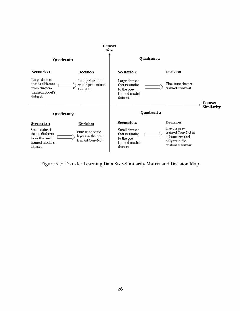
Two main factors should be considered when choosing the type of transfer learning to
perform on a new dataset. These factors are the size of the dataset and its similarity to
the original datasets on which the repurposed models were trained (Karpathy, 2017).
For small new datasets, the ConvNet should not be fine-tuned to avoid overfitting but
large datasets can be fine-tuned without the risk of overfitting. The various scenarios for
new datasets can be summarized as follows (Karpathy, 2017):
a) A small new dataset that is similar to the pre-trained ConvNet dataset- Due
to data similarity, the higher-level features in the ConvNet will be relevant to the
new dataset. The best approach in this case would be to use the pre-trained
ConvNet as a featurizer and only train a new linear classifier, i.e., freeze all the
other trainable layers.
25
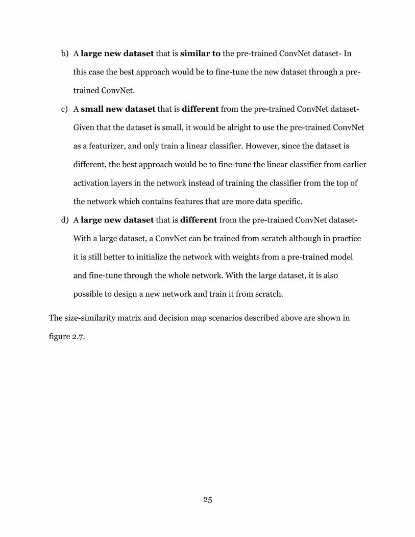
b) A large new dataset that is similar to the pre-trained ConvNet dataset- In
this case the best approach would be to fine-tune the new dataset through a pre-
trained ConvNet.
c) A small new dataset that is different from the pre-trained ConvNet dataset-
Given that the dataset is small, it would be alright to use the pre-trained ConvNet
as a featurizer, and only train a linear classifier. However, since the dataset is
different, the best approach would be to fine-tune the linear classifier from earlier
activation layers in the network instead of training the classifier from the top of
the network which contains features that are more data specific.
d) A large new dataset that is different from the pre-trained ConvNet dataset-
With a large dataset, a ConvNet can be trained from scratch although in practice
it is still better to initialize the network with weights from a pre-trained model
and fine-tune through the whole network. With the large dataset, it is also
possible to design a new network and train it from scratch.
The size-similarity matrix and decision map scenarios described above are shown in
figure 2.7.
26
Figure 2.7: Transfer Learning Data Size-Similarity Matrix and Decision Map
27
Chapter 3: Methodology
The purpose of this chapter is to discuss the development of a deep learning framework
for the early detection and continuous monitoring of crop diseases and its
implementation using high-resolution multispectral imagery and the transfer learning
methodology of deep learning. This approach enabled the use of small datasets to train
deep learning models. The selection of the best performing pre-trained deep learning
network for training crop and crop disease models for early detection and continuous
monitoring of crop diseases is also discussed.
The applicability and the rationale of using transfer learning for the studies undertaken
in this research are described in detail in this chapter. The model selection, data
collection, and data analysis methods are also described in this chapter.
3.1 Proposed Framework for Crop Disease Monitoring
Methods used in previous research to train crop and crop disease classification models
have mostly depended on the use of leaf images taken using hand-held digital cameras
and smartphones. Even though these types of images are easy to acquire, they are
inconsistent due to differences in camera angle and image background. The
development of models using leaf images is appropriate for the use-case where farmers
will eventually ingest such images of their diseased crops into their smartphones and
obtain an immediate diagnosis of the identified disease using a smartphone application.
The approach proposed for this framework is to use high-resolution and multispectral
whole canopy images of healthy and diseased crops taken from aerial platforms without

28
segmenting them into single-leaf images. The use of whole canopy images enables the
development of an automated diagnosis system that ingests new images as soon as they
are acquired (at the temporal resolution of the aerial imagery acquisition) and processes
them to detect, identify, and monitor crop and crop diseases continuously without
requiring the intervention of the farmer.
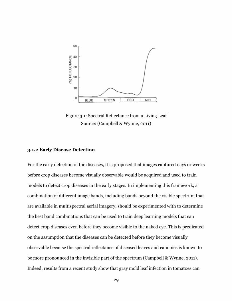
3.1.1 Spectral Behavior of Leaves and Canopies
Chlorophyll molecules in plants absorb up to 90% of incident sunlight in the blue and
red region of the visible spectrum for photosynthesis. The plants, however, reflect most
of the green light and only a small amount is absorbed in the visible region, hence the
appearance of green as the color of living plants to a human observer (Campbell &
Wynne, 2011). Although the reflectance of plant canopies is lower than that observed for
individual leaves, the relative decrease of the reflectance is considerably lower in the
infrared region than in the visible region of the spectrum. The spectral characteristics of
plants may, however, be affected by age, moisture availability, and diseases. Although
these changes occur in both the visible and the near infrared regions of the spectrum,
they are more pronounced in the near infrared region, as shown in Figure 3.1.
Reflectance changes in the near infrared region have been used to map the presence of
crop diseases and insect infestations (Campbell &. Wynne, 2011)
Given these differences in the spectral characteristics of healthy and diseased crops and
plants in the visible and invisible regions of the spectrum, the implementation of this
framework will enable the use of different reflectance characteristics of crop canopies
combined with machine learning to discriminate between healthy and diseased plants
even before the symptoms of the diseases become visually observable.
29
Figure 3.1: Spectral Reflectance from a Living Leaf
Source: (Campbell & Wynne, 2011)
3.1.2 Early Disease Detection
For the early detection of the diseases, it is proposed that images captured days or weeks
before crop diseases become visually observable would be acquired and used to train
models to detect crop diseases in the early stages. In implementing this framework, a
combination of different image bands, including bands beyond the visible spectrum that
are available in multispectral aerial imagery, should be experimented with to determine
the best band combinations that can be used to train deep learning models that can
detect crop diseases even before they become visible to the naked eye. This is predicated
on the assumption that the diseases can be detected before they become visually
observable because the spectral reflectance of diseased leaves and canopies is known to
be more pronounced in the invisible part of the spectrum (Campbell & Wynne, 2011).
Indeed, results from a recent study show that gray mold leaf infection in tomatoes can

30
be detected as early as nine hours after infection (long before visual symptoms appear)
using near infrared and red edge sensors (Fahrentrapp et al., 2019). The pre-disease
imagery should be categorized according to the time steps (e.g., number of days) they
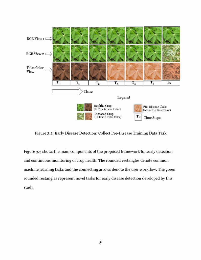
were captured before the diseases became visually observable, as shown in Figure 3.2.
The figure illustrates how the healthy and diseased crops would appear in natural color
and possibly in a hypothetical false color composite of bands extracted from an aerial
image. The first row (RGB View 1) shows images of a healthy crop, while the images in
the second row (RGB View 2) also show a healthy crop except the last image (TN) which
shows an image of a diseased crop as it would appear in natural color (RGB). The third
row (False Color View) is an example of how the second row would look like in a
hypothetical false color band combination where a pre-disease class exists. In this view,
the first three images (T0 to T2) represent the view of the healthy crop, the next three
images (T3 to T5) represent a pre-disease class as it would appear in the false color, while
the last image (TN) represents the same diseased crop shown in the second row as it
would appear in this hypothetical false color view.
Although only one pre-disease class is shown as an example here, many more classes
may be identified during model experimentation and training. The trained disease
classification models should be continuously updated to include any ‘newly-discovered’
early stage diseases classes.
31
Figure 3.2: Early Disease Detection: Collect Pre-Disease Training Data Task
Figure 3.3 shows the main components of the proposed framework for early detection
and continuous monitoring of crop health. The rounded rectangles denote common
machine learning tasks and the connecting arrows denote the user workflow. The green
rounded rectangles represent novel tasks for early disease detection developed by this
study.

32
Figure 3.3: Framework for Early Detection and Continuous Monitoring of Crop Diseases
This framework is intended for use by, for example, regional and national government
agencies to monitor crop health in large areas. Such agencies are expected to monitor
continuously the crop health of different crops during the crop-growing season for
seasonal crops and annually for perennial crops. The agencies should use trained crop
classification models at the beginning of the growing season to identify and map the
areas where specific crops are sown, and then deploy trained crop diseases classification
models to images covering only those areas planted with the identified crops. The
detailed description of the major components of the framework are as follows.
Collect Training Data. In order to train the crop and crop disease classification
models, the user should first collect training data. The data should be curated and
labeled by domain experts before training crop and crop disease classification models.

33
Train Models. The crop and crop disease classification models should be trained using
the latest and the best performing deep learning networks and the best band
combinations extracted from multispectral images as determined through continuous
experimentations to compare their performances.
Extract Crop Layers. The trained crop model is used to extract and map crop layers
from high resolution multispectral aerial imagery to depict areas planted with specific
crops. These crop areas should be continuously verified and updated to match ground-
truth data.
Deploy Crop Disease Trained Model. This trained model is deployed on the
extracted crop layers to predict the presence or absence of crop diseases in aerial
images. The model should be run each time a new set of aerial imagery is acquired
during the crop-growing season.
Detect Crop Disease. The trained model is used to detect the presence of crop
diseases.
Take Remedial Action. Remedial action is taken as soon as a disease is detected to
prevent crop damage and the spread of the disease. The mitigation actions taken should
be guided by crop disease experts.
Monitor/Improve Crop and Crop Disease Models. The models’ performance
should be continuously improved by adding new training data gathered through the
monitoring of the models’ predictions against the ground truth data.
Collect Pre-Disease Training Data. Once a crop disease is detected in an area, the
area’s imagery captured days or weeks prior to the time the disease was detected should
34
be used to train a pre-disease classification model. The pre-disease stage may exist in
situations where a disease may be present but not visible to the naked eye, which detects
the red, green, and blue bands (RGB). Since the original crop disease model was trained
on images with observable diseases, it is important to experiment and test whether some
diseases can be identified with band combinations other than RGB. An illustration of
this process is shown in Figure 3.2. The pre-disease training data may be collected in
time steps (T0 to TN as shown in Figures 3.2 and 3.3), where T0 occurs after the crop
disease model is deployed and TN occurs just before the disease is detected. The time
steps for collecting the data may vary from days to weeks based the frequency of
acquisition of new imagery and on expert knowledge on how specific crop disease
symptoms manifest themselves in the field.
Create New Pre-Disease Class/Classes. The number of new pre-disease classes
should be based on the time steps chosen for collecting pre-disease training data. These
classes represent the time-periods for early detection of diseases.
Train Pre-Disease Classification Model/Models. The number of models to train
should be determined based on the number of pre-disease classes that were created.
These models should be tested to determine whether the classes can be distinguished
from the healthy crop class and from each other. The earliest pre-disease image class
that could be distinguished from the healthy class should then be used as an indicator of
the possible time to detect a disease before it is visible to the naked eye.
Re-Train Crop Disease Classification Model to Include New Class/Classes.
Only those models that are distinct from the healthy class and from each other should be
35
used in the re-training process and hence be incorporated into the future crop-disease
classification model as new pre-disease class/classes.
3.2 Transfer Learning Using the Keras Python Library
The transfer learning technique of repurposing pre-trained deep convolutional neural
networks for custom tasks was used to train classification models in the studies
described in this chapter. The training of the deep learning networks was implemented
using the Keras Python deep learning API running on top of the TensorFlow
computational engine backend. Keras is a Python-based high-level deep learning
framework that provides an API to other deep learning frameworks to facilitate the
building of deep neural networks (François Chollet, 2015).
The architecture and weights of several pre-trained deep convolutional neural networks,
some of which were selected from previous winners of the ILSVRC challenge, are
integrated in the Keras library and new models are continuously added to the API. Most
of the winning networks of the ILSVRC challenge have been shown to generalize well to
images from outside the ImageNet dataset. These pre-trained networks can be used for
custom tasks such as predicting, extracting features, and fine-tuning other imagery
datasets (François Chollet, 2015).
3.3 Model Selection
Five convolutional neural networks, which were pre-trained on the ImageNet dataset
and made available through the Keras library, were selected for this study. The

36
performances of these models on the task of classifying crop diseases were compared in
the first study and the best performing network was selected and used in all the other
studies described in this chapter. The following is a brief description of the five selected
networks.
3.3.1 VGG16 and VGG19
The VGG network, which took the second position in the 2014 ILSVRC competition, was
developed by (Simonyan & Zisserman, 2014). The VGG network consists of 3x3
convolutional filters placed on top of each other and increasing in depth from 64 to 512.
The two VGG networks (VGG16 and VGG19) have very similar architectures that only
differ in the number of weight layers, where the VGG16 network has 16 while the VGG19
network has 19. Maximum pooling layers of size 2x2 are used to reduce the volume of
the input image through the depth of the network. Each of the final two fully connected
layers of the network has 4,096 nodes and the last one is finally connected to a Softmax
classifier, which outputs the probabilities of each class label. Due to the depth of the two
VGG networks and their many connected nodes, the models are relatively big in terms of
disk size (533MB for VGG16 and 574MB for VGG19) making it slow to train and deploy.
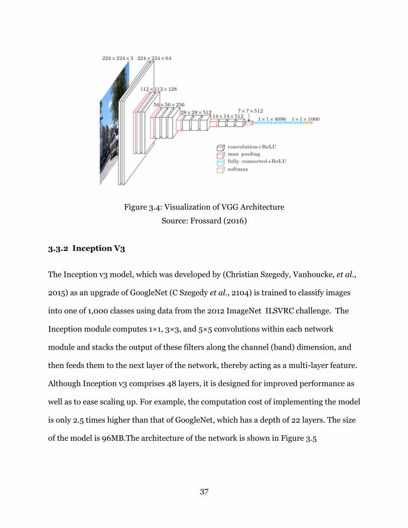
A visualization of the VGG16 network is shown in Figure 3.4.
37
Figure 3.4: Visualization of VGG Architecture
Source: Frossard (2016)
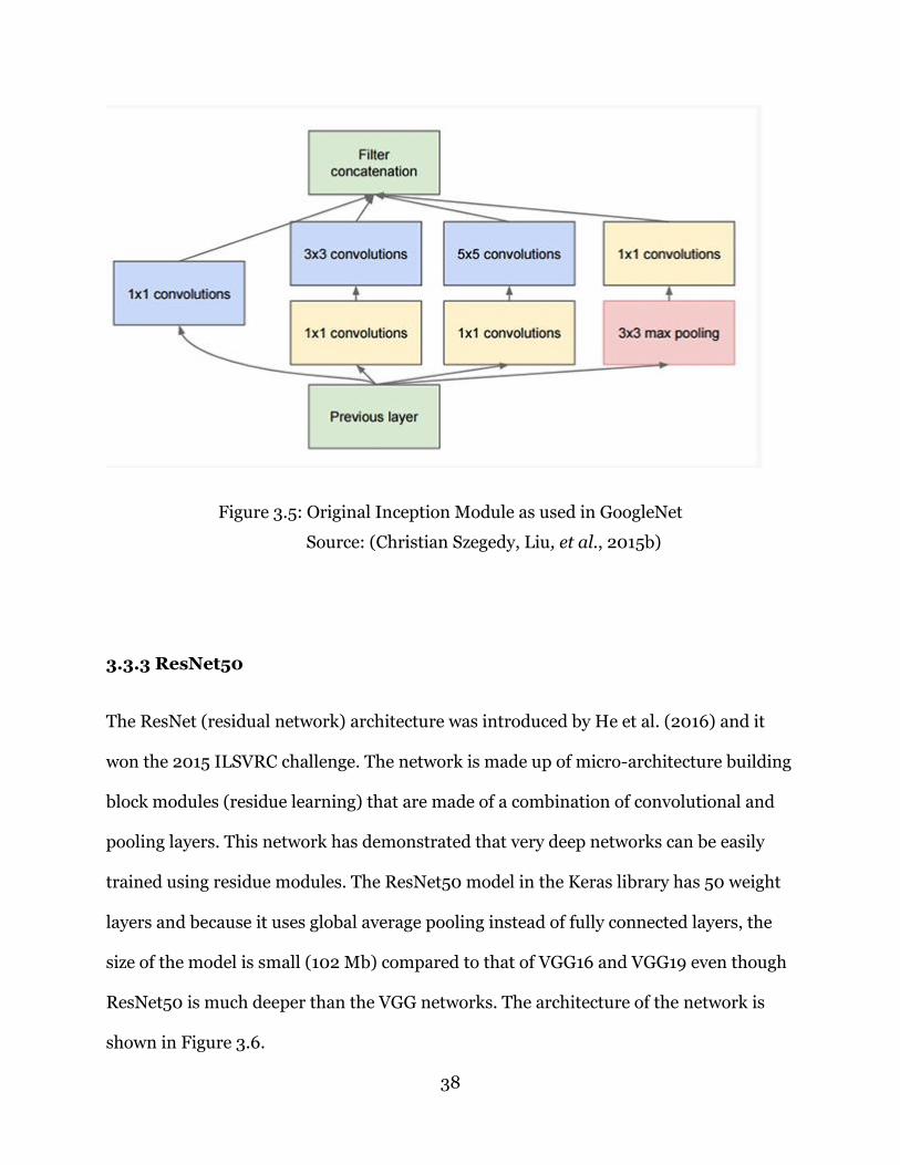
3.3.2 Inception V3
The Inception v3 model, which was developed by (Christian Szegedy, Vanhoucke, et al.,
2015) as an upgrade of GoogleNet (C Szegedy et al., 2104) is trained to classify images
into one of 1,000 classes using data from the 2012 ImageNet ILSVRC challenge. The
Inception module computes 1×1, 3×3, and 5×5 convolutions within each network
module and stacks the output of these filters along the channel (band) dimension, and
then feeds them to the next layer of the network, thereby acting as a multi-layer feature.
Although Inception v3 comprises 48 layers, it is designed for improved performance as
well as to ease scaling up. For example, the computation cost of implementing the model
is only 2.5 times higher than that of GoogleNet, which has a depth of 22 layers. The size
of the model is 96MB.The architecture of the network is shown in Figure 3.5
38
Figure 3.5: Original Inception Module as used in GoogleNet
Source: (Christian Szegedy, Liu, et al., 2015b)
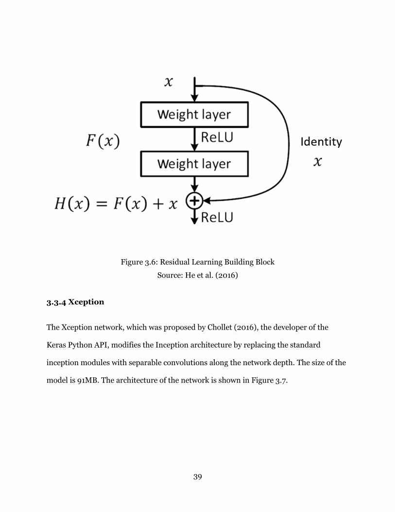
3.3.3 ResNet50
The ResNet (residual network) architecture was introduced by He et al. (2016) and it
won the 2015 ILSVRC challenge. The network is made up of micro-architecture building
block modules (residue learning) that are made of a combination of convolutional and
pooling layers. This network has demonstrated that very deep networks can be easily
trained using residue modules. The ResNet50 model in the Keras library has 50 weight
layers and because it uses global average pooling instead of fully connected layers, the
size of the model is small (102 Mb) compared to that of VGG16 and VGG19 even though
ResNet50 is much deeper than the VGG networks. The architecture of the network is
shown in Figure 3.6.
39
Figure 3.6: Residual Learning Building Block
Source: He et al. (2016)
3.3.4 Xception
The Xception network, which was proposed by Chollet (2016), the developer of the
Keras Python API, modifies the Inception architecture by replacing the standard
inception modules with separable convolutions along the network depth. The size of the
model is 91MB. The architecture of the network is shown in Figure 3.7.

40
Figure 3.7: The Xception Architecture.
Source: Chollet (2016)
3.3.5 Summary of Model Selection
These five pre-trained deep learning networks were used to train crop disease
classification models in the first study described in the following section. Model
performance was compared based on several metrics, as described in the data analysis
section later in this chapter, and the winning network was selected to train models for
all the other studies conducted in this dissertation.
The following is a description of the methods and procedures used to implement the
developed deep learning framework.
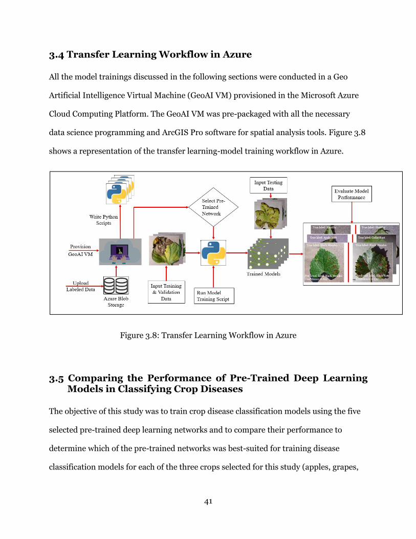
41
3.4 Transfer Learning Workflow in Azure
All the model trainings discussed in the following sections were conducted in a Geo
Artificial Intelligence Virtual Machine (GeoAI VM) provisioned in the Microsoft Azure
Cloud Computing Platform. The GeoAI VM was pre-packaged with all the necessary
data science programming and ArcGIS Pro software for spatial analysis tools. Figure 3.8
shows a representation of the transfer learning-model training workflow in Azure.
Figure 3.8: Transfer Learning Workflow in Azure
3.5 Comparing the Performance of Pre-Trained Deep Learning Models in Classifying Crop Diseases
The objective of this study was to train crop disease classification models using the five
selected pre-trained deep learning networks and to compare their performance to
determine which of the pre-trained networks was best-suited for training disease
classification models for each of the three crops selected for this study (apples, grapes,
42
and tomatoes) both individually and jointly. The best performing pre-trained model was
then used in the other studies described later in this chapter.
The crop diseases imagery dataset used for this study was curated by PlantVillage
("Plantvillage," 2017) and was downloaded from the CrowdAI data challenges platform
("Plantvillage Disease Classification Challenge," 2016) which hosted a “PlantVillage
Disease Classification Challenge” in 2016, whose goal was to use the plant disease
images to develop algorithms for diagnosing plant diseases. The dataset contains images
of crop leaves that were taken from leaves plucked from different experimental fields at
research stations in several Land Grant Universities in the USA. The leaves were placed
on gray or black paper backgrounds and positioned outside (Hughes & Salathé, 2015)
where their images were taken under full light using a point and shoot camera (Sony
DSC - Rx100/13 20.2 megapixels) set on automatic mode. Additional images of the
leaves were taken under a range of outside conditions (sunny to cloudy) to mimic the
conditions under which crop growers would normally take their images using a
smartphone. The images are released under the Creative Commons license ("Creative
Commons," 2018) which requires that algorithms developed using the data be freely
shared.
This study used only a subset of the PlantVillage imagery dataset to train models for
classifying diseases of apples, grapes, and tomatoes. This subset dataset contained
13,860 RGB color images of healthy and diseased leaves of the crops each measuring
256 X 256 pixels. A sample of the images is shown in Figure 3.9. Although the pre-
trained deep learning networks selected for this study were originally trained using
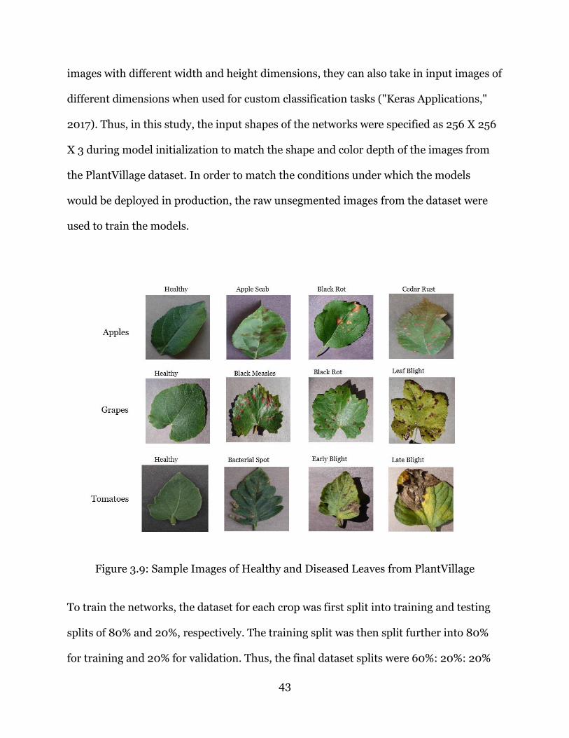
43
images with different width and height dimensions, they can also take in input images of
different dimensions when used for custom classification tasks ("Keras Applications,"
2017). Thus, in this study, the input shapes of the networks were specified as 256 X 256
X 3 during model initialization to match the shape and color depth of the images from
the PlantVillage dataset. In order to match the conditions under which the models
would be deployed in production, the raw unsegmented images from the dataset were
used to train the models.
Figure 3.9: Sample Images of Healthy and Diseased Leaves from PlantVillage
To train the networks, the dataset for each crop was first split into training and testing
splits of 80% and 20%, respectively. The training split was then split further into 80%
for training and 20% for validation. Thus, the final dataset splits were 60%: 20%: 20%

44
for training, validation, and testing, respectively for each crop. The summary of the total
number of healthy and diseased leaf images and the number of training images per
health/disease class for each of the three selected crops is shown in Table 3.1.
Table 3.1: Crop Health/Disease Classes Labels and Training Data Summary
As Table 3.1 shows, the health and disease classes were not equally represented in the
dataset as some classes had more images than other classes. This class imbalance can
lead to trained models that are biased toward overfitting into the classes that have more
training data. For the studies carried out in this dissertation, the problem of class
imbalance, and hence model bias, was addressed by computing class weights and
apportioning proportionately more weight to the underrepresented classes during
model training.
45
The fine-tuning method of transfer learning was selected to train the pre-trained
networks in this study because the data available was considered small and dissimilar to
the ImageNet dataset on which the pre-trained networks were trained. This is because
the ImageNet dataset falls into the Quadrant 3 of the size-similarity matrix scenarios
described in Section 2.5 and as shown in Figure 2.7 in Chapter 2. The fine-tuning
process implemented for this study is described in the following section.
3.5.1 The Fine-Tuning Process
The fine-tuning of the pre-trained networks was implemented according to the following
steps.
1) Remove the fully connected (dense) layers at the top of the pre-trained network
(classifier) and load the convolutional base of the network.
2) Replace the removed network’s top with a new custom classifier of randomly
initialized fully connected layers.
3) Freeze the convolutional base of the network. Freezing ensures that the weights of the
convolutional base of the pre-trained network do not change during the fine-tuning
process.
4) Train the newly added custom classifier layers using end-to-end training with a data
augmentation method, where the images are augmented and passed through the
whole network during training.
5) Unfreeze some top layers of the convolutional base of the network and perform a
second end-to-end training pass until a satisfactory classification model is achieved.
46
This step ensures that the unfrozen convolutional base layers will now be jointly
trained with the fully connected layers that were initially trained in step four.
6) Save the trained model. In this final step, the trained model is saved and can then be
used for inference to classify crop disease on new, previously unseen, imagery.
The added custom classifier (step 2) for this study consisted of a dense layer with 256
nodes, a rectified linear unit (ReLU) activation layer, and a dropout rate of 0.5. The
specifications for this added classifier were a slight modification of the one proposed by
(F Chollet, 2017). The number of output classes was set to the number of disease and
health classes for the crops in the dataset used in this study.
Since the custom classifier layers added on top of the network are randomly initialized,
it is crucial to freeze the convolutional base before training the custom classifier to
prevent the propagation of large weights through the network, as this would destroy the
data patterns that the base of the pre-trained network had previously learned. Thus, the
purpose of freezing the convolutional base of the pre-trained network was to ensure that
the weights that the layers in the base had previously learned were not updated during
the process of fine-tuning the custom classifier added on top of the base.
To ensure a fair comparison of the performances of the five pre-trained networks, the
number of layers that were unfrozen in the convolution base of each pre-trained
network were chosen such that they contained approximately the same total number of
parameters. This was done to guarantee that an almost equal number of parameters
were fine-tuned in each network. However, due to the differences in the pre-trained
networks’ architecture, it was not possible to match layers in the different networks such
that the number of parameters available for fine tuning in each network was exactly
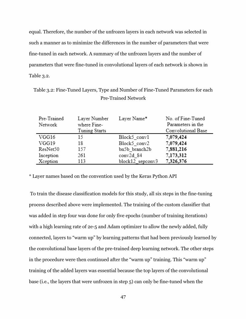
47
equal. Therefore, the number of the unfrozen layers in each network was selected in
such a manner as to minimize the differences in the number of parameters that were
fine-tuned in each network. A summary of the unfrozen layers and the number of
parameters that were fine-tuned in convolutional layers of each network is shown in
Table 3.2.
Table 3.2: Fine-Tuned Layers, Type and Number of Fine-Tuned Parameters for each
Pre-Trained Network
* Layer names based on the convention used by the Keras Python API
To train the disease classification models for this study, all six steps in the fine-tuning
process described above were implemented. The training of the custom classifier that
was added in step four was done for only five epochs (number of training iterations)
with a high learning rate of 2e-5 and Adam optimizer to allow the newly added, fully
connected, layers to “warm up” by learning patterns that had been previously learned by
the convolutional base layers of the pre-trained deep learning network. The other steps
in the procedure were then continued after the “warm up” training. This “warm up”
training of the added layers was essential because the top layers of the convolutional
base (i.e., the layers that were unfrozen in step 5) can only be fine-tuned when the
48
classifier on top of them has had some training (i.e., not randomly initialized).
Otherwise the patterns that the layers had previously learned would be destroyed by the
large error signal that would be propagated through the network by the un-trained
classifier during the second training pass in step 5 (F Chollet, 2017).
During this second training pass of the fine-tuning process, each network was trained
for 15 epochs using a learning rate of 1e-5, which was lower than the learning rate that
was used in step four. It was necessary to use a lower learning rate in this step to limit
the size of the modifications made to the previously-learned weights of the layers that
were being fine-tuned since large updates to those previously-learned representations
would destroy them (F Chollet, 2017). Figure 3.10 represents the process of fine-tuning
the pre-trained networks undertaken in this study using the VGG16 network as an
example.
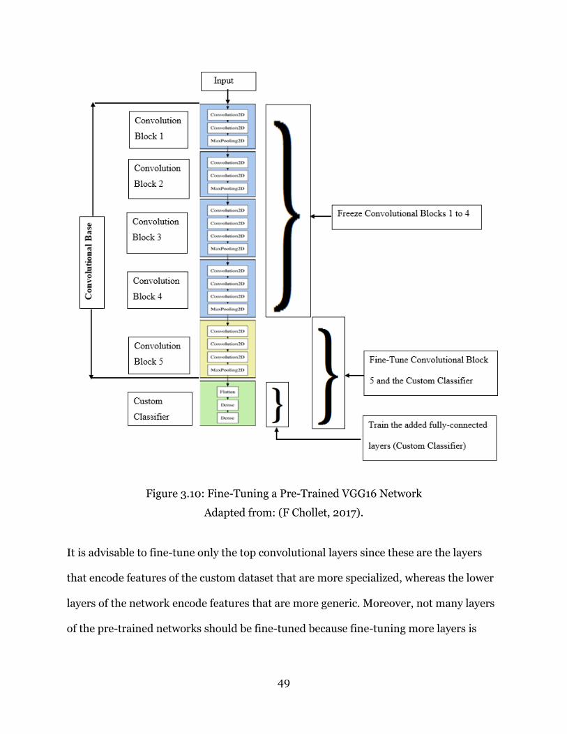
49
Figure 3.10: Fine-Tuning a Pre-Trained VGG16 Network
Adapted from: (F Chollet, 2017).
It is advisable to fine-tune only the top convolutional layers since these are the layers
that encode features of the custom dataset that are more specialized, whereas the lower
layers of the network encode features that are more generic. Moreover, not many layers
of the pre-trained networks should be fine-tuned because fine-tuning more layers is

50
computationally costly and it also increases the risk of overfitting because it means more
parameters would be trained with the small custom dataset (F Chollet, 2017).
To further prevent the risk of overfitting during model training, considering that the
datasets obtained for these studies were small, Keras data augmentation techniques
were used to randomly transform the original training data on-the-fly during model
training. Because of these random transformations, the network “sees” different
variations of the original data at every epoch during model training. This type of data
augmentation is analogous to generating additional training data to ensure that the
network does not “see” the same images over and over, to the extent that it captures
even spurious patterns of the training data but fails to generalize to unseen data, thus
leading to less accurate predictions (F Chollet, 2017). In this study, data augmentation
was implemented by applying a range of the following random geometric
transformations to the input images: rotation, shear, zoom, horizontal shift, width, and
height shift. The Keras Image Data generator method was used to make these
transformations yield batches of images from disk storage, eliminating the need for
holding the entire dataset in memory, which is desirable, especially if the training
computer has limited memory.
3.6 Comparing the Performance of Crop Classification Models Trained on Different Three-Band Combination Images
The purpose of this study was to train crop classification models using different three-
band combination training images extracted from four-band imagery and to compare
their performances to determine which band-combination model was best suited for:

51
(i) Classifying each single crop (apples, corn, grapes, and tomatoes) separately, and
(ii) Classifying three crops (corn, grapes, and tomatoes), and four crops (apples, corn,
grapes, and tomatoes) together.
The following is a description of the sources and the preparation processes for the data
used in this study.
3.6.1 Cropland Data Layer (CDL)
The Cropland Data Layer (CDL) is a geo-referenced, raster layer that provides a crop-
specific land cover map for the continental USA. The data layer is created annually using
moderate-resolution satellite imagery and is verified against the ground-truth through
an extensive agricultural network of data collection agencies. The CDL data is hosted by
the United States Department of Agriculture’s (USDA) National Agricultural Statistics
Service at CropScape (United States Department of Agriculture, 2018).
The CDLs by State (2007 – 2017) for California were downloaded from the USDA
Geospatial Data Gateway ("Geospatial Data Gateway," 2018). The raster layers
contained pixels for all the crops cultivated in the state for the years 2007 to 2017, but
only the layers for years 2014 and 2016 were used in this study. The raster masks for
each crop of interest in this study (apples, corn, grapes, and tomatoes) were extracted
from the downloaded layer. Each crop’s raster layer was then visually examined and
areas that had large acreages under each crop were randomly selected as Areas of
Interest (AOI) for each crop, as shown in Figure 3.11. The 2016 CDL layers were used for
corn, grapes, and tomatoes, while for apples, the 2014 layer was used because the 2016
CDL layer for apples showed only very few areas under the crop during that year.

52
The selected Apples AOI is in Kern county; the corn AOI is in San Joaquin, Contra
Costa, Solano, and Sacramento counties; the grapes AOI in San Joaquin county; and the
tomatoes AOI is in Fresno county.
Figure 3.11: California Cropland Data Layers (CDLs) Areas of Interest (AOI)

53
3.6.2 National Agriculture Imagery Program (NAIP) Imagery
The National Agriculture Imagery Program’s (NAIP) “leaf-on” aerial imagery is collected
annually in the continental United States during the crop-growing season. Currently the
highest spatial resolution of California NAIP imagery is 0.6 meters, while the highest
spectral resolution is 4 bands. These bands are Red, Green, Blue, and Near Infrared
(RGBI). An individual NAIP image tile covers 3.75 x 3.75 minutes with an additional
300-meter buffer on the sides (Farm Service Agent, 2018), which is approximately 7.5
km X 6.5 km ground area. The selection of the NAIP imagery to download was guided by
AOI as determined by the CDL layer.
Data for training the classification models to compare the performance of the 3-band
combination classification models were extracted from the NAIP imagery in ArcGIS
Desktop 10.6.1 and ArcGIS Pro 2.4.1 according to the procedure in Section 3.6.3. All the
NAIP images were downloaded from the ("California Natural Resources Agency," 2019).
3.6.3 Procedure for Extracting Training Data for Each Crop
1. Use the CDL layer to select and define an Area of Interest for each crop.
2. Download the four-band NAIP imagery for the AOI and the year of interest (years
2014 for apples, and 2016 for the other 3 crops NAIP images were downloaded for
this study).
3. Create a four-band mosaic raster layer covering the AOI from the downloaded NAIP
imagery.
54
4. Extract the four unique three-band color combinations (RGB, IGB, RGI, and RIB
raster layers) from the four-band NAIP mosaic raster layer.
5. Use the CDL for the crop and the extracted RGB mosaic layer to map and create a
training samples layer representing polygons of randomly selected areas on the
ground that are covered by the crop (the RGB layer represents the natural color layer
and thus was used as a guide to identify the crop on the ground in the NAIP images).
6. Use the training samples layer as a clip layer to extract training samples from each of
the four three-band layers.
7. Convert the training samples into training data (image chips) and extract the data for
deep learning.
8. Repeat the above process for the other crops in the study.
Figure 3.12 shows the four-band mosaic layer that was created from NAIP images
covering the selected AOI for grapes in this study, while the process of extracting grapes
training samples using the procedure described above is shown in Figure 3.13.

55
Figure 3.12: Four-Band NAIP Mosaic for Grapes AOI
The following are the four unique three-band color-combination raster layers that were
extracted from the four-band NAIP mosaic raster layer in step 4 above.
(i) IGB- Near Infrared, Green, and Blue
(ii) RGB- Red, Green, and Blue
(iii) RGI- Red, Green, and Near Infrared
(iv) RIB- Red, Near Infrared, and Blue

56
Figure 3.13: Extracting Grapes Training Samples from Four 3-Band Raster Layers
3.6.4 Training Single and Multi-Crop Classification Models
To help make random selections of areas on the ground that were covered by a
particular crop, the extracted RGB layer (natural color layer) and the CDL layer for that
crop were zoomed-in and toggled on/off to reveal and match the ground-truth areas that
were covered by the crop to the image in the RGB layer. Thus, the CDL layer was used in
this process as the reference map, that is, the ground-truth to show the exact areas
covered by the crop. To create a training samples map for each crop, only areas covered
with mature canopies of the crop were selected and mapped on the RGB layer; areas
with newly planted or pruned crops were avoided.

57
The images extracted from each of the 3-band raster layers were converted into smaller
image chips with a resolution of 256 X 256 pixels to meet the shape requirements of the
inputs to the pre-trained deep learning networks. After the chips for the RGB raster
layer were extracted, the above procedure was repeated using the same training samples
map for the crop to extract and convert the images for the other three-band raster
layers. Since the chips were created using the same training samples map for each crop,
the image for an area covered by any one chip was thus extracted four times with four
different band combinations.
After the chips were extracted, they were examined manually and those that contained
extraneous material such as roads, pathways and fences were removed from the chip’s
dataset. The extracted training data was then split into train, validation, and testing sets
using the same ratios as those described in Section 3.4. A summary of the extracted data
is shown in Table 3.3.

58
Table 3.3: Three-Band Combinations Classes Training Data Summary
Note: Red (R), Green (G), Blue (B), and Near Infrared (I)
Based on the number of training images per class, this dataset is also considered small.
However, the data was deemed similar to the ImageNet dataset, which includes images
of plant, flora, and plant-life categories. Thus, the dataset for this study lies in Quadrant
4 of the size similarity matrix decision map shown in Figure 2.7 in Chapter 2.
Accordingly, a fine-tuning method known as feature extraction with data augmentation
(Chollet, 2017), was applied. Using this end-to-end training method, augmented data
was passed through the entire pre-trained network (VGG16) but only the added top fully
connected layers were fine-tuned. To achieve acceptable model accuracies, training of
the added custom classifier was conducted for 10 epochs, instead of the 5 epochs in step

59
4 of the fine-tuning process in the previous study as described in Section 3.5.1. However,
the same optimizer and learning rate (Adam optimizer, learning rate of 2e-5) were used.
After the training in this stage was completed, the next step (5) of the fine-tuning
process was skipped because only the custom classifier requires training in this fine-
tuning method. The trained model was then saved.
Once all the training samples were extracted and converted, crop classification models
were trained as follows:
(i) Single crop classifiers – image chips from each of the four three-band
combinations were treated as separate classes and used to train four single
crop classification models, one for each of the four crops— apples, corn,
grapes, and tomatoes. For example, the classification model for apples
consisted of the four classes: Apples IGB, Apples RGB, Apples RGI, and
Apples RIB.
(ii) Multi-crop classifiers – image chips from each of the corresponding three-
band color combination for each crop were treated as separate classes and
used to train multi-crop classification models for three crops (corn, grapes,
and tomatoes), and four crops (apples, corn, grapes, and tomatoes). For
example, the three classes for one of the four multi-crop classification models
(for three crops) were: Corn RGB, Grapes RGB, and Tomatoes RGB as shown
in Figure 3.14. This was repeated for the other remaining three-band
combinations (IGB, RGI, and RIB) and for the classification models for four
crops.

60
The performances of the separate classifiers were then compared to determine which
three-band combination was best suited for classifying single and multiple crops,
respectively.
Figure 3.14: Extracted Training Data for the Three Crops RGB Classification Model
The best-performing three-band combination model for the three crops multi-crop
classifier (corn, grapes, and tomatoes) was then used to classify previously unseen NAIP
images as described in the following section.
3.7 Using the Best-Performing Multi-Crop Classification Model to Classify NAIP Imagery
Using the 2016 California CDL layers for corn, grapes, and tomatoes, a separate AOI
located in San Joaquin and Stanislaus counties (All 3 Crops AOI) containing the three
crops (corn, grapes, and tomatoes) was selected. The NAIP images for this AOI were
then downloaded. Next, the best-performing band combination layer for the three-
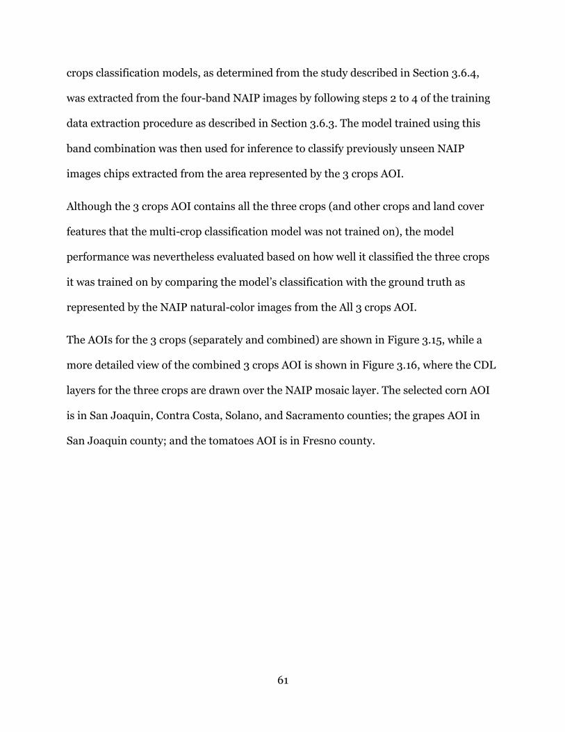
61
crops classification models, as determined from the study described in Section 3.6.4,
was extracted from the four-band NAIP images by following steps 2 to 4 of the training
data extraction procedure as described in Section 3.6.3. The model trained using this
band combination was then used for inference to classify previously unseen NAIP
images chips extracted from the area represented by the 3 crops AOI.
Although the 3 crops AOI contains all the three crops (and other crops and land cover
features that the multi-crop classification model was not trained on), the model
performance was nevertheless evaluated based on how well it classified the three crops
it was trained on by comparing the model’s classification with the ground truth as
represented by the NAIP natural-color images from the All 3 crops AOI.
The AOIs for the 3 crops (separately and combined) are shown in Figure 3.15, while a
more detailed view of the combined 3 crops AOI is shown in Figure 3.16, where the CDL
layers for the three crops are drawn over the NAIP mosaic layer. The selected corn AOI
is in San Joaquin, Contra Costa, Solano, and Sacramento counties; the grapes AOI in
San Joaquin county; and the tomatoes AOI is in Fresno county.

62
Figure 3.15: Map of Areas of Interest (AOIs) for Separate and Combined Crops
Figure 3.16: All 3 Crops AOI CDL layers over the NAIP Mosaic Layer
63
3.8 Data Analysis
The performances of the networks were compared based on the performance metrics
listed below. The models that displayed well-fit characteristics during training and
achieved the highest scores in Precision, Recall, Accuracy, and F1 scores on the test
datasets, were considered as the best performing.
1) Precision – Measures the correctly classified images as a fraction of all the images
predicted to belong to a specific class and is expressed mathematically as:
Precision = True Positives / (True Positives + False Positives).
2) Recall – Measures the correctly classified images as a fraction of all the images
that belong to a specific class and is expressed mathematically as:
Recall = True Positives/ (True Positives + False Negatives).
3) Classification Accuracy – Measures the correctly classified images as a fraction of
the total number of predictions made and is expressed mathematically as:
Classification Accuracy = Number of Correct Predictions / Total Number of
Predictions.
4) F1 Score – Measures the harmonic mean of Precision and Recall and it can be
used as a single score to summarize the model performance. The score is
expressed mathematically as:
F1 Score = (2 * Precision * Recall) / (Precision + Recall)
5) Confusion Matrix – Confusion matrices show the number (or percentage for
normalized confusion matrices) of correctly and incorrectly predicted labels for
each class and they are used to show whether a classifier has a bias toward certain
classes.
64
6) Training and Validation Curves – The training and validation accuracy and loss
curves are used to diagnose whether trained models are under-fit, over-fit, or
well-fit.
Both precision (Type I error) and recall (Type II error) were considered equally
important for all the models. As such, models with high precision values were desirable
to minimize the misclassification of healthy crops as diseased (and thus would
recommend the need to apply mitigation solutions to healthy crops) in the case of crop
disease models, and to minimize misclassification of bands and crops in the case of crop
classification models. Similarly, models with high recall values were desirable to
minimize the misclassification of diseased crops as healthy (and thus fail to recommend
the need to apply mitigation solutions to diseased crops) in the case of crop disease
models, and to minimize misclassification of bands and crops in the case of crop
classification models.
3.9 Summary
The purpose of this chapter was to outline the research methodology and methods used
to investigate the research objectives. A framework for the continuous monitoring of
crop diseases was developed and implemented using the transfer learning methodology
of deep learning to train crop and crop diseases classification models. A description of
methods and procedures for deep learning model selection, data acquisition, data pre-
processing, and models training gave the detailed specifics of how the studies in this
dissertation were conducted. The goal of the following chapter is to present the results

65
of these studies and to demonstrate how the methodology and procedures described in
this chapter were followed.
66
Chapter 4: Data Analysis and Results
This chapter presents the results of the studies that were implemented following the
proposed deep learning framework and using transfer learning methods to train deep
learning classification models. The studies were conducted to answer the following
research questions.
1: Which of the five selected pre-trained deep learning models is best suited for training
crop diseases classification models?
2. Which three-band combination extracted from four-band multispectral images is best
suited for classifying single crops?
3. Which three-band combination extracted from four-band multispectral images is best
suited for classifying multiple crops?
4. How well does the best three-band combination multi-crop classifier generalize in
classifying new imagery?
For all the studies described here, the models were trained on a GPU powered by an
NVIDIA Tesla K80 card and Intel Xeon E5-2690 v3 (Haswell) processor with 12 CPU
cores and 24 vCPUs running on a Windows Virtual Machine (VM) instance in the
Microsoft Azure cloud platform. The training was done with the Keras Python API
running on top of a TensorFlow backend. All the models were trained using Adam
Optimizer, a categorical cross-entropy loss function, and batch sizes of 30. The
performance of the models was evaluated based on the performance metrics described
in Section 3.7.

67
All the Cropland data and NAIP imagery processing were done using ArcGIS 10.6.1
Desktop and ArcGIS Pro 2.4.1.
Figure 4.1 shows a screen shot of the Jupyter Notebook Python code used to split the
original datasets into training, validation, and testing datasets, while Figure 4.2 shows
the screenshot for the code used for data augmentation and model training. The
complete Jupyter Notebooks containing markup annotations and the computer code
used to train the models for all the studies undertaken in this research can be accessed
through the following GitHub link: https://github.com/kimanim/DissCode/.

68
Figure 4.1: Screenshot Jupyter Notebook Python Code for Splitting Datasets
(Inset shows the resultant directory structure after apples dataset split)
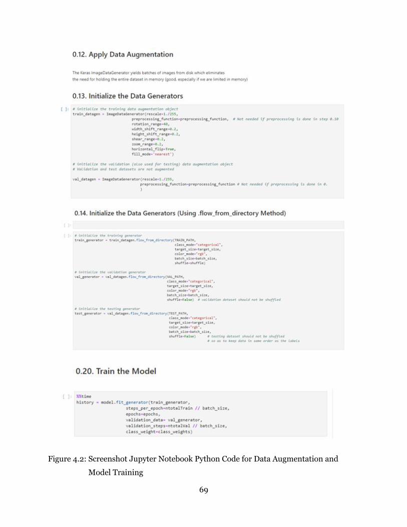
69
Figure 4.2: Screenshot Jupyter Notebook Python Code for Data Augmentation and
Model Training

70
4.1 Comparing the Performance of Pre-Trained Deep Learning Networks
The fine-tuning method of transfer learning was used to compare performance of five
pre-trained networks (VGG16, VGG19, ResNet50, InceptionV3, and Xception) in
classifying crop diseases of apples, grapes, and tomatoes using the PlantVillage dataset.
Using this method, the convolutional base of each pre-trained network was frozen, and a
custom classifier of fully connected layers was added on top of the frozen base. The
custom classifier was trained for 5 epochs with a learning rate of 2e-5. Some layers of
the convolutional base were then unfrozen and fine-tuned together with the added
classifier for 15 epochs with a lower learning rate of 1e-5.
Based on the performance metrics results shown in Table 4.1, the models trained on the
VGG16 network outperformed all the other models in classifying the diseases and health
classes of all the three crops separately and jointly except in the testing accuracy for
grapes where the VGG19 model achieved a testing accuracy (measured using the test
dataset) of 99.11% compared to 98.98% for VGG16. However, the two models were tied
on the other performance metrics where they each achieved values of 0.99 for each of
the metrics. The worst performing network was ResNet50, which attained the lowest
scores for all the metrics across all the trained models.
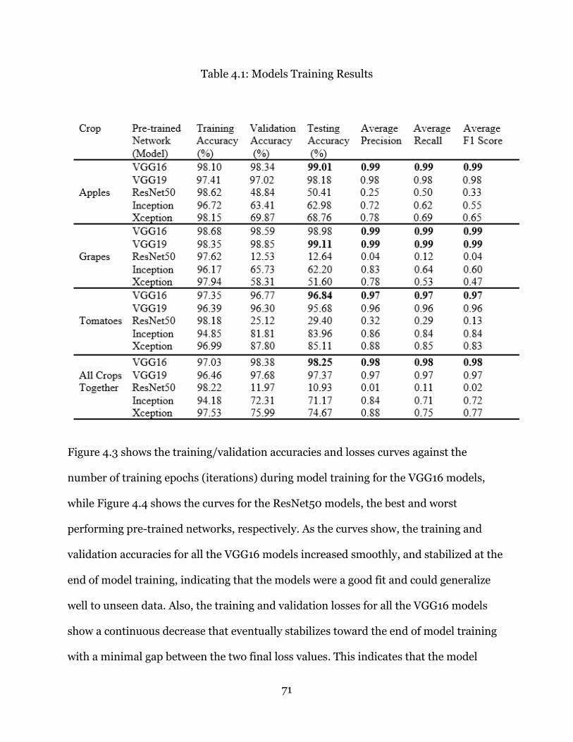
71
Table 4.1: Models Training Results
Figure 4.3 shows the training/validation accuracies and losses curves against the
number of training epochs (iterations) during model training for the VGG16 models,
while Figure 4.4 shows the curves for the ResNet50 models, the best and worst
performing pre-trained networks, respectively. As the curves show, the training and
validation accuracies for all the VGG16 models increased smoothly, and stabilized at the
end of model training, indicating that the models were a good fit and could generalize
well to unseen data. Also, the training and validation losses for all the VGG16 models
show a continuous decrease that eventually stabilizes toward the end of model training
with a minimal gap between the two final loss values. This indicates that the model
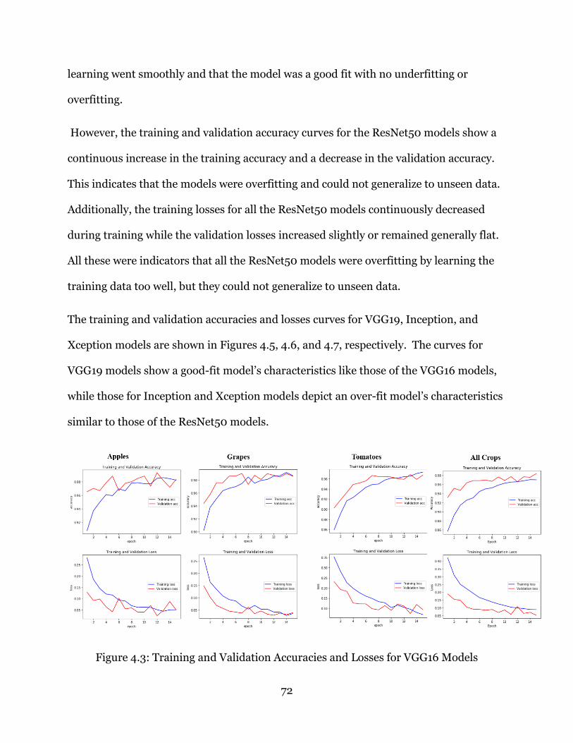
72
learning went smoothly and that the model was a good fit with no underfitting or
overfitting.
However, the training and validation accuracy curves for the ResNet50 models show a
continuous increase in the training accuracy and a decrease in the validation accuracy.
This indicates that the models were overfitting and could not generalize to unseen data.
Additionally, the training losses for all the ResNet50 models continuously decreased
during training while the validation losses increased slightly or remained generally flat.
All these were indicators that all the ResNet50 models were overfitting by learning the
training data too well, but they could not generalize to unseen data.
The training and validation accuracies and losses curves for VGG19, Inception, and
Xception models are shown in Figures 4.5, 4.6, and 4.7, respectively. The curves for
VGG19 models show a good-fit model’s characteristics like those of the VGG16 models,
while those for Inception and Xception models depict an over-fit model’s characteristics
similar to those of the ResNet50 models.
Figure 4.3: Training and Validation Accuracies and Losses for VGG16 Models
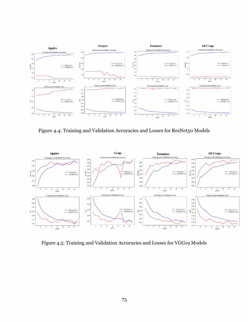
73
Figure 4.4: Training and Validation Accuracies and Losses for ResNet50 Models
Figure 4.5: Training and Validation Accuracies and Losses for VGG19 Models

74
Figure 4.6: Training and Validation Accuracies and Losses for Inception Models
Figure 4.7: Training and Validation Accuracies and Losses for Xception Models
A more detailed view of the models’ performance can be obtained by examining the
confusion matrices that show, for example, the classes which were difficult for the
trained models to confuse or distinguish from other classes. The rows in a confusion
matrix correspond to the true labels (classes), while the columns show the predicted

75
labels. The diagonal cells show the percentage of the samples the trained model
predicted correctly (percentage of samples in which true and predicted labels are equal).
The confusion matrices for the VGG16 single-crop disease classification models are
shown in Figure 4.8, while the matrix for VGG16 all crops disease classification model is
shown in Figure 4.9. Figure 4.8 shows that the VGG16 model correctly identified (100%)
all the healthy and black rot images in apples, and all the black rot and leaf blight
images in grapes. The model was, however, only able to identify correctly 86% of all
early blight leaf images in tomatoes and it tended to confuse that disease with late blight
in 12% of the cases.
Figure 4.8: Confusion Matrices for VGG16 Single Crop Disease Classification Models
(See Table 3.1 for the full names of the labels)
The VGG16 all crops disease classification model confusion matrix (Figure 4.9) shows
only slight variations in classification accuracy from those attained by the single crop
classification models. The figure also shows that this model (unlike some of the other
all-crops models) did not confuse diseases across crops, with all the misclassifications

76
occurring only among diseases of the same crop as shown by the overlain colored
rectangles.
Figure 4.9: Confusion Matrix for VGG16 All Crops Disease Classification Model
Some of the other network models (VGG19, Inception, and Xception) confused diseases
across crops, while the ResNet50 model classifications were not established due to poor
training performance as shown in the confusion matrices for the all the other networks’
single and all-crops disease classification models (see Appendix).
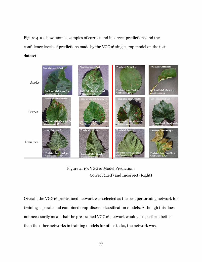
77
Figure 4.10 shows some examples of correct and incorrect predictions and the
confidence levels of predictions made by the VGG16 single crop model on the test
dataset.
Figure 4. 10: VGG16 Model Predictions
Correct (Left) and Incorrect (Right)
Overall, the VGG16 pre-trained network was selected as the best performing network for
training separate and combined crop-disease classification models. Although this does
not necessarily mean that the pre-trained VGG16 network would also perform better
than the other networks in training models for other tasks, the network was,

78
nevertheless, selected for use in the all the other transfer learning studies undertaken in
this research. Those results are presented in the following sections.
4.2 Comparing the Performance of Different Band Combination Crop Classification Models
The crop classification models in this study were trained using the four unique three-
band color combinations training images extracted from four-band NAIP imagery. Their
performances were then compared to determine the band combination model was best
suited for classifying single and multiple crops. The models in this study were trained
using the VGG16 pre-trained network, the best-performing network in the training of
crop-disease classification models as shown in the results presented in Section 4.1.
Given that the NAIP images used in this study have four bands, and the images in the
ImageNet dataset that were used to train the pre-trained networks have only three
bands (RGB), it was necessary to investigate whether better-performing crop
classification models could be achieved by fine-tuning the pre-trained network using
images of other band combinations. The results would then be used to recommend the
best band combinations for future training of crop classification models.
4.2.1 Using Three-Band Combination Models to Classify Single Crops
Table 4.2 shows the performance results of the three-band combination single crop
classification models. The results show that RGI and RIB band combination models
were the best performing for apples, grapes, and tomatoes with precision, recall, and F1
scores of between 0.97 and 0.98 for apples, and 1.00 scores for grapes and tomatoes. All
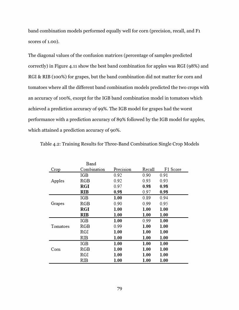
79
band combination models performed equally well for corn (precision, recall, and F1
scores of 1.00).
The diagonal values of the confusion matrices (percentage of samples predicted
correctly) in Figure 4.11 show the best band combination for apples was RGI (98%) and
RGI & RIB (100%) for grapes, but the band combination did not matter for corn and
tomatoes where all the different band combination models predicted the two crops with
an accuracy of 100%, except for the IGB band combination model in tomatoes which
achieved a prediction accuracy of 99%. The IGB model for grapes had the worst
performance with a prediction accuracy of 89% followed by the IGB model for apples,
which attained a prediction accuracy of 90%.
Table 4.2: Training Results for Three-Band Combination Single Crop Models

80
Figure 4.11: Confusion Matrices for Single Crop Classification Models
Using Different Band Combinations
4.2.2 Using Three-Band Combination Models to Classify Three Crops
The performance results of the three-band combination models for classifying three
crops (corn, grapes, and tomatoes) are shown in Table 4.3. The results show that the
models trained on the RGB and RIB band combinations performed better than the other
band combinations achieving 98.48% accuracy, 0.99 average precision, and 0.98 for
average recall and F1 for the RGB; and 98.48% accuracy, 0.98 average precision, and
0.98 for average recall and F1 scores for the RIB model.

81
The confusion matrices shown in Figure 4.12 show that the most accurate models for
corn were RGB, RGI, and RIB (98%); RGB and RIB for grapes (98%); RGB and RGI
(100%) for tomatoes. The RGB and RIB models confused corn and grapes with tomatoes
at (2%) or less, while the RGI model confused grapes with tomatoes in 4% of the cases.
The worst performing model was the IGB model, which confused corn with tomatoes at
7% and grapes with tomatoes in 4% of the cases.
Table: 4.3: Training Results for Three-Band Combination Three Crops Models

82
Figure 4.12: Confusion Matrices for Three Crops Classification Models
Using Different Band Combinations
The confusion matrices show that the best models for corn were RGB and RGI attaining
a classification accuracy of 98%. For grapes, the best models were RGB and RIB with a
classification accuracy of 98%, while RGB and RGI were the best-performing models for
tomatoes with a classification accuracy of 100%. Overall, the RGB band combination
model was selected as the best performing for classifying three crops (corn, grapes, and
tomatoes).
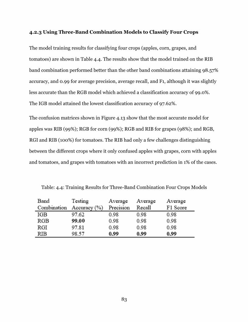
83
4.2.3 Using Three-Band Combination Models to Classify Four Crops
The model training results for classifying four crops (apples, corn, grapes, and
tomatoes) are shown in Table 4.4. The results show that the model trained on the RIB
band combination performed better than the other band combinations attaining 98.57%
accuracy, and 0.99 for average precision, average recall, and F1, although it was slightly
less accurate than the RGB model which achieved a classification accuracy of 99.0%.
The IGB model attained the lowest classification accuracy of 97.62%.
The confusion matrices shown in Figure 4.13 show that the most accurate model for
apples was RIB (99%); RGB for corn (99%); RGB and RIB for grapes (98%); and RGB,
RGI and RIB (100%) for tomatoes. The RIB had only a few challenges distinguishing
between the different crops where it only confused apples with grapes, corn with apples
and tomatoes, and grapes with tomatoes with an incorrect prediction in 1% of the cases.
Table: 4.4: Training Results for Three-Band Combination Four Crops Models

84
Figure 4.13: Confusion Matrices for Four Crops Classification Models
Using Different Band Combinations
The confusion matrices (Figure 4.13) also show that the RIB model mostly performed
better for each crop (considered separately) than the other models, with its lowest
classification accuracy of 98% for corn and grapes, and a 100% classification accuracy
for tomatoes.
4.4 Making Inferences from Unseen NAIP Imagery
The RGB model, which was selected as the best performing three crops classifier in
Section 4.2.2 was used to classify previously unseen NAIP imagery extracted from a
study area containing three crops (corn, grapes, and tomatoes). A total of 856 inference

85
image chips were extracted and their labels were generated using the CDL layers as the
ground-truth for the inference imagery area of interest. The RGB model achieved an
inference accuracy of 98.55%.
Figure 4.14 shows some examples of correct and incorrect predictions, and the
confidence levels of predictions made by the RGB three crops classifier on the inference
dataset.
Figure 4.14: RGB Three Crops Model Predictions
Correct (Left) and Incorrect (Right)
4.5 Summary
This chapter presented the detailed findings of implementing the proposed deep
learning framework for early detection and continuous monitoring of crop diseases. The
use of the transfer learning approach in deep learning to train deep learning models
86
with limited data was demonstrated, with the results showing that the VGG16 pre-
trained network performed better in classifying crop diseases than the other pre-trained
networks examined in this study. The results also show that using other bands outside
the visible spectrum improved the single and multiple crop classification accuracies of
deep learning models, with models incorporating the Near Infrared band generally
performing better than models trained with the traditional visible spectrum band
combination of RGB. Overall, the best performing models for single and multiple crops
were those trained on RGB and RIB band combinations, and the worst were those
trained on the IGB band combination.

87
Chapter 5: Discussion and Conclusions
Advances made in deep learning have made it possible to train highly accurate image
classification models using large datasets. Although recent studies have shown that deep
models are more accurate and can be trained efficiently (Huang et al., 2016), they are
costly and difficult to train because of challenges such as vanishing gradients and
internal covariate shifts which emerge as the model depth increases (Nielsen, 2015).
Some of the strategies that have been proposed for dealing with such challenges include
batch normalization (Christian Szegedy et al., 2016), skip connections (He et al., 2016),
and optimization methods (Le et al., 2011).
Training deep learning models is also challenging because they require large amounts of
training data, which may be unavailable and/or costly to acquire. This challenge can be
addressed by using a transfer learning strategy (Pan & Yang, 2010), which entails the re-
use of deep learning models which have been pre-trained on large datasets for a specific
task (for example, classify plants), to transfer the knowledge gained by the models
during the pre-training process to other tasks (for example, classify crop diseases) where
large amounts of data may be unavailable. By using transfer learning, accurate crop
disease classification models can be trained and deployed quickly thus enabling the
monitoring and early application of mitigating factors to control crop diseases and avert
food crises at regional and national levels.
Various image processing methods such as low-level feature extraction (Aduwo et al.
(2010), traditional machine learning (Dubey & Jalal, 2011), shallow neural networks
88
(Abdullakasim et al., 2011), and deep learning (Mohanty et al., 2016) have been applied
over time to identify and classify crop diseases, with each new method achieving better
performance than the previous ones. Deep learning crop-disease classification models
have particularly attained high classification accuracies in recent studies (Mohanty et
al., 2016). The application of transfer learning to train deep neural networks for crop
disease classification has also been tried recently, and studies show that the strategy
improves classification accuracy and reduces model training time (Ramcharan et al.
(2017); (Too et al., 2019).
The first study in this dissertation extends previous research on transfer learning by
fine-tuning only a few layers of five state-of-the-art deep learning pre-trained networks
(VGG16, VGG19, ResNet50, Inception, and Xception) instead of fine-tuning the entire
network, as in previous studies, and comparing their performance in classifying crop
diseases.
The results show that the VGG16 pre-trained deep learning convolution neural network
outperformed the other four pre-trained networks that were investigated in the study.
This result was unexpected given that the VGG16 network was the shallowest of all the
networks used in the study whereas studies have shown that deeper networks (He et al.,
2016) with sparser architectures and fewer parameters perform better than shallower
networks (Christian Szegedy, Liu, et al., 2015b). In another study comparing the
performance of pre-trained networks using the entire PlantVillage plant diseases
dataset, Too et al., (2019) show that ResNet and Densenet (with 152 and 121 layers,
respectively) performed better than VGG16, which has 16 layers. In their study,
however, they implemented the transfer learning strategy of fine-tuning the entire
89
network, instead of fine-tuning only a few layers in the convolutional bases of the
networks as was done in this study.
One possibility why the deeper networks did not perform as expected in this study may
be attributed to the decision to fine-tune an almost equal number of parameters in each
pre-trained network. Perhaps a better strategy would be to fine-tune an equal
percentage of the t0tal number of trainable parameters in each network’s convolutional
base. The number of layers to fine-tune in each network would then be chosen based on
this percentage instead of fine-tuning an equal number of parameters in each network.
The percentages of trainable parameters fine-tuned in this study were approximately
48.1%, 35.4%, 33.5%, 33.0%, and 35.2% for VGG16, VGG19, ResNet50, Inception, and
Xception networks, respectively (as shown in Table 5.1). Thus, it is probable that the
deeper networks did not perform well because a lower ratio of their trainable
parameters were fine-tuned compared to those of the VGG16 model, implying this study
was biased toward the VGG16 network and that the deeper networks were
disadvantaged because their “depth benefits” were not exploited in full. This could have
resulted from the fact that the number of layers selected for fine-tuning in the deeper
networks were too shallow such that many deeper layers that had already learned
specialized features of the original dataset (that the networks were pre-trained on) were
left intact, hence preventing the networks from learning the full features of the new
custom dataset during the fine-tuning process (F Chollet, 2017).
Although the results of this study seem to be inconsistent with other studies cited above
that show that deeper networks perform better than shallower networks, an apples-to-
apples comparison of these studies may be inappropriate because of the differences in

90
the fine-tuning strategies employed. Morever, even the performance of a given network
may differ depending on when the comparative studies were conducted because the
network developers ocassionally update and modify the original architectures of their
pre-trained netwoks.
Table 5.1: Fine-Tuned Parameters as a Percentage of Total Parameters
Even though the VGG16 network performed better than the other pre-trained networks,
it still made some crop-disease classification errors. These errors may be attributed to
the visual similarities of the diseases. For example, while the VGG16 model correctly
identified (100%) all the healthy and black rot images in apples, and all the black rot and
leaf blight images in grapes (as shown by the VGG16 model confusion matrices in Figure

91
4. 8), it was only able to correctly identify 86% of all early blight leaf images in tomatoes.
Furthermore, the model tended to confuse the disease with late blight disease in 12% of
the cases. A visual examination of a random sample of leaf images of the two diseases
(Figure 5.1) shows that the diseases appear very similar to the naked eye implying that
an untrained observer may have difficulties distinguishing between the two diseases.
Besides confusing the model, it can also be argued that this similarity may result in
labelling errors, where leaf images of one disease may be incorrectly labelled as
belonging to the other disease category thereby confusing the model during training.
Figure 5.1: Visual Similarities of Early and Late Blight Tomato Diseases

92
Another reason that may have contributed to the confusion of the diseases is the fact
that the images were not categorized according to disease severity levels. It may well be
possible for one disease at a given severity level to be visually more similar to another
disease than to the same disease at another severity level leading to classification errors.
The findings of this study show that pre-trained convolutional networks can be
repurposed by fine-tuning a few layers in their convolutional bases through transfer
learning, to successfully train new image classification models with limited custom data
that may be different from the original dataset on which the networks were trained. This
is significant because it enables the fast training of models for new tasks and facilitates
the quick deployment of such models for urgent needs, such as detection and mitigation
of crop diseases.
The results of the studies comparing the use of different band combinations to train
crop classification models show that using the Near Infrared band improved the
performance of single and multiple crop classification models, with models
incorporating the band generally performing better than models trained with the
traditional visible spectrum band combination of RGB. These results were expected
given that plant canopies have brighter reflectance in the near infrared region than in
the visible region of the spectrum (Campbell & Wynne, 2011).
Whereas the predominant band combination of imagery used to train crop and plant
classification models is RGB (Red, Green, and Blue), which is the natural color
combination and the most common (and least expensive) of the available image-
capturing sensors, these results show that crop classification models can be improved by
training them with images combining bands in the visible and the near infrared parts of

93
the spectrum. Models trained on the RIB (Red, Near Infrared, and Blue) band
combination were found to be the best for classifying single and multiple crops, while
those trained on the IGB (Near Infrared, Green, and Blue) band combination had the
worst performance.
These results imply that there is no need to train stand-alone single crop classifiers
using the best band combination for each individual crop since one multiple crop
classifier trained on the RIB band combination can achieve equally good classification
results for all the crops. Thus, for the crops investigated in this study (apples, corn,
grapes, and tomatoes), it would be less expensive and faster to train and deploy only one
multiple crop classifier trained on the RIB band combination instead of extracting the
best band combination for each crop.
The development of crop and crop disease classification models using leaf images in
previous studies by Ramcharan et al. (2017) and Mwebaze and Owomugisha (2016) was
deemed appropriate for the use-case where crop health model training uses easy-to-
acquire leaf images and diseases are monitored by individual farmers using hand-held
devices, such as cellphones, at the farm level. The approach taken by this research is to
train the models using whole canopy aerial images and to monitor the diseases by
ingesting imagery acquired through satellites and other aerial platforms for fast wide-
area diagnosis of crop health. This workflow will enable the development of an
automated diagnosis system that ingests new images as soon as they are acquired (at the
temporal resolution of the aerial imagery acquisition) and processes them to detect,
identify, and monitor the diseases continuously without requiring the intervention of
the farmer.

94
5.1 Conclusions
The objectives of this research were to develop methods and workflows for using
multispectral aerial imagery and different band combinations extracted from the
multispectral imagery to build deep learning models for early detection and continuous
monitoring of crop diseases. This research developed a framework for building the
models and investigated how it could be implemented for the following specific
purposes: to train crop disease classification models using transfer learning and natural
color images, propose how false color images can be used to train deep learning models
for early crop disease detection and classification, and to determine the best-suited
spectral band combination for training deep learning models for detecting and
classifying single and multiple crops jointly and separately using transfer learning.
5.1.1 Crop Disease Classification
While the initially proposed goal of this study was to determine the best band
combinations for training deep learning models for early-detection and classification of
cassava diseases, this goal could not be achieved due to unavailability of the required
data. However, the overarching goal of the study was nevertheless achieved by
developing methods and workflows using available data for other crops as a proxy for
the originally proposed study as summarized below.
In this study, five pre-trained deep learning convolutional neural networks were fine-
tuned and evaluated on their performance in classifying crop diseases using data from

95
PlantVillage. The networks evaluated were VGG16, VGG19, ResNet50, Inception, and
Xception. The results of this study show that the model trained on the VGG16 network
(the shallowest of the networks evaluated) was the best-performing for crop disease
classification attaining scores as high as 99.01% for testing accuracy and 0.99 for
average precision and recall in the apple diseases classification model. The VGG16
models exhibited smooth-learning characteristics during training and displayed good fit
model characteristics with no signs of underfitting or overfitting. These results show
that transfer learning can be used with limited custom data to train successfully crop-
disease classification models, thus obviating the need of going through the costly and
time-consuming process of acquiring a large corpus of custom data that is required to
train deep learning models from scratch.
5.1.2 Band Combination Classification Models
Different crop classification models were trained using the four unique three-band
combination color images extracted from four-band (Red, Green, Blue, and Near
Infrared) imagery from the National Agriculture Imagery Program (NAIP). The trained
models were compared to determine which three-band color combination was best
suited for classifying single and multiple crops.
The results show that models trained with RGI and RIB band combination images were
the best performing classifiers for single crops (classification accuracy >=98%), while
RGB and RIB models achieved the best performance in classifying three crops
(classification accuracy = 98.48%). The RIB model achieved the best overall
performance among the four-crop classification models (classification accuracy
=98.57%). The IGB models had the worst performance in all the cases. The overall

96
results indicate that RIB is the best band combination for training single and multiple
classification models for apples, corn, grapes, and tomatoes.
The results of these studies show that the transfer learning strategy can also be applied
to train highly accurate models for classifying single and multiple crops using three-
color band combination imagery extracted from multispectral aerial imagery.
As high spatial and spectral resolution aerial images become less expensive due to the
proliferation of aerial imagery providers, this researcher anticipates that the proposed
approach of using full canopy crop imagery (as opposed to using leaf images) to train
crop disease models will become affordable and scalable enabling regional and state
governments or other private providers in underserved regions to monitor crop health
over large geographic regions and provide information to farmers as a service. This
scalability will enable the detection of crop diseases over wider regions, which is an
improvement of the currently available solutions that are geared toward enabling
farmers to monitor crop diseases at the individual farm level. Moreover, monitoring
crop disease over large geographic areas is a better approach for controlling crop
diseases because it enables the application of mitigation factors over wide areas instead
of putting the onus on single farmers to control crop diseases at individual farm
holdings as that may not stop the diseases from spreading to other farms.
5.2 Significance of Research Findings
Prior research has shown that transfer learning can be used to fine-tune whole pre-
trained deep learning models for classifying crop diseases using natural color imagery.
This research contributes to the previous research through the development of a deep

97
learning framework and workflows for determining the best band combinations of
multispectral imagery for training crop and crop-disease classification models through
transfer learning, i.e., by fine-tuning only a few layers of the pre-trained deep learning
models. Further, this research introduces a novel method of using false color band
combinations to detect and classify crop diseases before they become visible to the
naked eye. This early detection of “invisible” crop diseases is expected to facilitate the
application of crop-disease prevention measures at an early stage, and thus reduce the
cost of treating diseases and increase crop yields. The framework and the workflow
developed in this research can also be adapted and scaled for monitoring other
situations such as, water stress in crops, crop yields, forest health, illegal logging, water
levels, etc.
5.3 Limitations of Research
One of the initially proposed goals of this research was to determine the best band
combinations (extracted from high resolution multispectral canopy imagery) for
training classification models for early detection of cassava diseases in sub-Saharan
Africa, where the crop is a major source of carbohydrates and income for smallholder
farmers, especially women. This goal was not achieved due to unavailability of the
required multispectral aerial cassava canopy imagery and the unavailability of crop
disease calendars showing the dates when diseases were detected in the intended areas
of study. Even low-resolution images could not be acquired because this research could
not establish the dates when the crops in the chosen areas of study were affected by the
diseases. Thus, this study was limited to using the available natural color leaf images of

98
other crops to test the viability of using transfer learning to train crop-disease
classification models.
Similarly, only four-band multispectral images (Red, Blue, Green, and Near Infrared)
were available for the training of crop classification models. Due to this limitation of the
number of spectral bands available, the studies were limited to only the investigation of
the performance of three-band combination models.
Lastly, the crop-classification training data were extracted from field crops with varying
ages and development stages. Since crop reflectance varies with age and stage of
development, it was not possible to determine how this variability affected the
performance of the trained crop classification models.
5.4 Recommendations for Future Research
As multispectral imagery becomes readily available, this researcher recommends that
the following further studies be undertaken as a follow-up of the findings of this
research and to bridge some of the gaps identified herein.
1. Using multispectral canopy imagery (rather than leaf images) to determine the
best band combinations (three bands or more) for training models to classify
crops and plants; and for early detection of crop and plant diseases.
2. Train multi-label models for classifying crops and their age or stages of growth.
These studies should be geared toward improving the crop classification models
to enable the monitoring of other critical crop-age dependent variables such as
moisture stress.
99
3. Determine the best band combinations (three bands or more) for training single-
and multi-label classification models for crop disease stages prior to the visual
appearance of symptoms, and crop-disease severity levels.
100
References
Abdullakasim, W., Powbunthorn, K., Unartngam, J., & Takigawa, T. (2011). An Images
Analysis Technique for Recognition of Brown Leaf Spot Disease in Cassava.
Tarım Makinaları Bilimi Dergisi, 7(2).
Aduwo, J. R., Mwebaze, E., & Quinn, J. A. (2010). Automated Vision-Based Diagnosis
of Cassava Mosaic Disease. Paper presented at the Industrial Conference on
Data Mining-Workshops.
Alexander, S. A., & Palmer, C. J. (1999). Forest Health Monitoring in the United States:
First Four Years. Environmental Monitoring and Assessment, 55(2), 267-277.
doi:Doi 10.1023/A:1005905310299
Barbedo, J. G. A. (2013). Digital Image Processing Techniques for Detecting,
Quantifying and Classifying Plant Diseases. SpringerPlus, 2(1), 660.
Bay, H., Ess, A., Tuytelaars, T., & Van Gool, L. (2008). Speeded-up Robust Features
(Surf). Computer vision and image understanding, 110(3), 346-359.
Brownlee, J. (2017). A Gentle Introduction to Transfer Learning for Deep Learning.
Retrieved from https://machinelearningmastery.com/transfer-learning-for-
deep-learning/
California Natural Resources Agency. (2019, 2019). Retrieved from
http://gisarchive.cnra.ca.gov/iso/
Campbell, J. B., & Wynne, R. H. (2011). Introduction to Remote Sensing: Guilford
Press.
Chollet, F. (2015). Keras: The Python Deep Learning Library.
101
Chollet, F. (2017). Deep Learning with Python: Manning Publications Co.
Collins, C. B., Beck, J. M., Bridges, S. M., Rushing, J. A., & Graves, S. J. (2017). Deep
Learning for Multisensor Image Resolution Enhancement. 37-44.
doi:10.1145/3149808.3149815
Creative Commons. (2018). Retrieved from https://creativecommons.org/licenses/by-
sa/3.0/
Dalal, N., & Triggs, B. (2005). Histograms of Oriented Gradients for Human Detection.
Paper presented at the Computer Vision and Pattern Recognition, 2005. CVPR
2005. IEEE Computer Society Conference on.
Deng, J., Dong, W., Socher, R., Li, L.-J., Kai, L., & Li, F.-F. (2009). Imagenet: A Large-
Scale Hierarchical Image Database. 248-255. doi:10.1109/cvpr.2009.5206848
Dubey, S. R., & Jalal, A. S. (2014). Adapted Approach for Fruit Disease Identification
Using Images. arXiv preprint arXiv:1405.4930.
F.A.O. (2019a). Global Agriculture Towards 2050.
F.A.O. (2019b). Plant Health and Food Security. Retrieved from
http://www.fao.org/3/a-i7829e.pdf
Fahrentrapp, J., Ria, F., Geilhausen, M., & Panassiti, B. (2019). Detection of Gray Mold
Leaf Infections Prior to Visual Symptom Appearance Using a Five-Band
Multispectral Sensor. Frontiers in plant science, 10, 628.
Farm Service Agent, U. (2018). Naip Imagery. Retrieved from
https://www.fsa.usda.gov/programs-and-services/aerial-photography/imagery-
programs/naip-imagery/

102
Franke, J., & Menz, G. (2007). Multi-Temporal Wheat Disease Detection by Multi-
Spectral Remote Sensing. Precision Agriculture, 8(3), 161-172.
doi:10.1007/s11119-007-9036-y
Geitgey, A. (2017). Imagenet Classes. Retrieved from
https://gist.github.com/ageitgey/4e1342c10a71981d0b491e1b8227328b
Geospatial Data Gateway. (2018). Retrieved from https://datagateway.nrcs.usda.gov/
Gibson, D., Burghardt, T., Campbell, N., & Canagarajah, N. (2015). Towards
Automating Visual in-Field Monitoring of Crop Health. Paper presented at the
Image Processing (ICIP), 2015 IEEE International Conference on.
He, K., Zhang, X., Ren, S., & Sun, J. (2016). Deep Residual Learning for Image
Recognition. Paper presented at the Proceedings of the IEEE Conference on
Computer Vision and Pattern Recognition.
Hughes, D., & Salathé, M. (2015). An Open Access Repository of Images on Plant Health
to Enable the Development of Mobile Disease Diagnostics. arXiv preprint
arXiv:1511.08060.
Imagenet. (2018). Retrieved from http://image-net.org/
Jia, Y., Shelhamer, E., Donahue, J., Karayev, S., Long, J., Girshick, R., . . . Darrell, T.
(2014). Caffe: Convolutional Architecture for Fast Feature Embedding. Paper
presented at the Proceedings of the 22nd ACM international conference on
Multimedia.
Karpathy, A. (2017). Cs231n Convolutional Neural Networks for Visual Recognition.
Retrieved from http://cs231n.github.io/transfer-learning/
Keras Applications. (2017). Keras Documentation. Retrieved from
https://keras.io/applications/
103
Krizhevsky, A., Sutskever, I., & Hinton, G. E. (2012). Imagenet Classification with Deep
Convolutional Neural Networks. Paper presented at the Advances in neural
information processing systems.
Long, J., Shelhamer, E., & Darrell, T. (2015). Fully Convolutional Networks for
Semantic Segmentation. Paper presented at the Proceedings of the IEEE
Conference on Computer Vision and Pattern Recognition.
Lowe, D. G. (2004). Distinctive Image Features from Scale-Invariant Keypoints.
International Journal of Computer Vision, 60(2), 91-110. doi:Doi
10.1023/B:Visi.0000029664.99615.94
Mohanty, S. P., Hughes, D. P., & Salathe, M. (2016). Using Deep Learning for Image-
Based Plant Disease Detection. Front Plant Sci, 7, 1419.
doi:10.3389/fpls.2016.01419
Mwebaze, E., & Owomugisha, G. (2016). Machine Learning for Plant Disease Incidence
and Severity Measurements from Leaf Images. Paper presented at the Machine
Learning and Applications (ICMLA), 2016 15th IEEE International Conference
on.
Nielsen, M. A. (2015). Neural Networks and Deep Learning (Vol. 25): Determination
press San Francisco, CA, USA:.
Pan, S. J., & Yang, Q. (2010). A Survey on Transfer Learning. IEEE Transactions on
knowledge and data engineering, 22(10), 1345-1359.
Plantvillage. (2017). Retrieved from www.plantvillage.org/
Plantvillage Disease Classification Challenge. (2016, 2018). Retrieved from
https://www.crowdai.org/challenges/plantvillage-disease-classification-
challenge
104
Puig, E., Gonzalez, F., Hamilton, G., & Grundy, P. (2015). Assessment of Crop Insect
Damage Using Unmanned Aerial Systems- a Machine Learning Approach.
Ramcharan, A., Baranowski, K., Mcclowsky, P., Ahmed, B., Legg, J., & Hughes, D.
(2017). Using Transfer Learning for Image-Based Cassava Disease Detection.
arXiv preprint arXiv:1707.03717.
Rosebrock, A. (2017). Deep Learning for Computer Vision with Python (1st Edition
ed.): PyImageSearch.
Schmidhuber, J. (2015). Deep Learning in Neural Networks: An Overview. Neural
Netw, 61, 85-117. doi:10.1016/j.neunet.2014.09.003
Seelan, S. K., Laguette, S., Casady, G. M., & Seielstad, G. A. (2003). Remote Sensing
Applications for Precision Agriculture: A Learning Community Approach.
Remote Sensing of Environment, 88(1-2), 157-169.
doi:10.1016/j.rse.2003.04.007
Simonyan, K., & Zisserman, A. (2014). Very Deep Convolutional Networks for Large-
Scale Image Recognition. arXiv preprint arXiv:1409.1556.
Siricharoen, P., Scotney, B., Morrow, P., & Parr, G. (2016). A Lightweight Mobile System
for Crop Disease Diagnosis. 9730, 783-791. doi:10.1007/978-3-319-41501-7_87
Sladojevic, S., Arsenovic, M., Anderla, A., Culibrk, D., & Stefanovic, D. (2016). Deep
Neural Networks Based Recognition of Plant Diseases by Leaf Image
Classification. Comput Intell Neurosci, 2016, 3289801.
doi:10.1155/2016/3289801
Szegedy, C., Liu, W., Jia, Y., Sermanet, P., Reed, S., Anguelov, D., . . . Rabinovich, A.
(2015a). Going Deeper with Convolutions. Paper presented at the Proceedings of
the IEEE conference on computer vision and pattern recognition

105
Szegedy, C., Liu, W., Jia, Y., Sermanet, P., Reed, S., Anguelov, D., . . . Rabinovich, A.
(2015b). Going Deeper with Convolutions. Paper presented at the Proceedings of
the IEEE conference on computer vision and pattern recognition
Szegedy, C., Liu, W., Jia, Y., Sermanet, P., Reed, S., Anguelov, D., . . . Rabinovich, A.
(2104). Going Deeper with Convolutions. arXiv preprint arXiv:1409.4842, 1409.
Szegedy, C., Vanhoucke, V., Ioffe, S., Shlens, J., & Wojna, Z. (2015). Rethinking the
Inception Architecture for Computer Vision. Proceedings of the IEEE Conference
on Computer Vision and Pattern Recognition.
Szegedy, C., Vanhoucke, V., Ioffe, S., Shlens, J., & Wojna, Z. (2016). Rethinking the
Inception Architecture for Computer Vision. Paper presented at the Proceedings
of the IEEE Conference on Computer Vision and Pattern Recognition.
Too, E. C., Yujian, L., Njuki, S., & Yingchun, L. (2019). A Comparative Study of Fine-
Tuning Deep Learning Models for Plant Disease Identification. Computers and
Electronics in Agriculture, 161, 272-279.
United States Department of Agriculture, U. (2017). Aerial Detection Survey:
Methodology. Retrieved from https://www.fs.usda.gov/detail/r5/forest-
grasslandhealth/?cid=stelprdb5429568
United States Department of Agriculture, U. (2018). National Agricultural Statistics
Service Cropland Data Layer. Retrieved from
https://nassgeodata.gmu.edu/CropScape/

106
Xiao, Q., & Mcpherson, E. G. (2005). Tree Health Mapping with Multispectral Remote
Sensing Data at Uc Davis, California. Urban Ecosystems, 8(3-4), 349-361.
doi:10.1007/s11252-005-4867-7
Zeiler, M. D., & Fergus, R. (2014). Visualizing and Understanding Convolutional
Networks. Paper presented at the European conference on computer vision.

107
Appendix
Figure A1: Confusion Matrices for VGG19 Single Crop Disease Classification Models
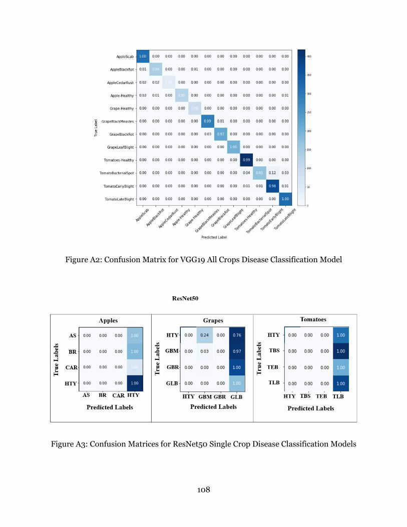
108
Figure A2: Confusion Matrix for VGG19 All Crops Disease Classification Model
Figure A3: Confusion Matrices for ResNet50 Single Crop Disease Classification Models

109
Figure A4: Confusion Matrix for ResNet50 All Crops Disease Classification Model
Figure A5: Confusion Matrices for Inception Single Crop Disease Classification Models

110
Figure A6: Confusion Matrix for Inception All Crops Disease Classification Model

111
Figure A7: Confusion Matrices for Xception Single Crop Disease Classification Models
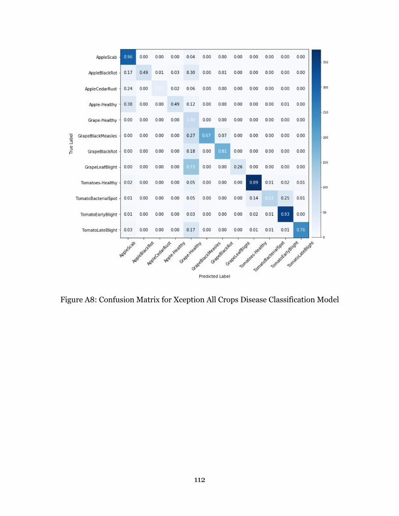
112
Figure A8: Confusion Matrix for Xception All Crops Disease Classification Model