deep feature learning for eeg recordings - arxiv · izontal and vertical electrooculography (eog)...

Under review as a conference paper at ICLR 2016

DEEP FEATURE LEARNING FOR EEG RECORDINGS

Sebastian Stober, Avital Sternin, Adrian M. Owen & Jessica A. GrahnThe Brain and Mind InstituteUniversity of Western OntarioLondon, ON, Canada{sstober,asternin,adrian.owen,jgrahn}@uwo.ca

ABSTRACT

We introduce and compare several strategies for learning discriminative fea-tures from electroencephalography (EEG) recordings using deep learning tech-niques. EEG data are generally only available in small quantities, they are high-dimensional with a poor signal-to-noise ratio, and there is considerable variabil-ity between individual subjects and recording sessions. Our proposed techniquesspecifically address these challenges for feature learning. Cross-trial encodingforces auto-encoders to focus on features that are stable across trials. Similarity-constraint encoders learn features that allow to distinguish between classes by de-manding that two trials from the same class are more similar to each other than totrials from other classes. This tuple-based training approach is especially suitablefor small datasets. Hydra-nets allow for separate processing pathways adapting tosubsets of a dataset and thus combine the advantages of individual feature learning(better adaptation of early, low-level processing) with group model training (bet-ter generalization of higher-level processing in deeper layers). This way, modelscan, for instance, adapt to each subject individually to compensate for differencesin spatial patterns due to anatomical differences or variance in electrode posi-tions. The different techniques are evaluated using the publicly available Open-MIIR dataset of EEG recordings taken while participants listened to and imaginedmusic.

1 INTRODUCTION

Over the last decade, deep learning techniques have become very popular in various applica-tion domains such as computer vision, automatic speech recognition, natural language process-ing, and bioinformatics where they produce state-of-the-art results on various tasks. At the sametime, there has been very little progress investigating the application of deep learning in cogni-tive neuroscience research, where these techniques could be used to analyze signals recorded withelectroencephalography (EEG) – a non-invasive brain imaging technique that relies on electrodesplaced on the scalp to measure the electrical activity of the brain. EEG is especially popular for thedevelopment of brain-computer interfaces (BCIs), which work by identifying different brain statesfrom the EEG signal.

Working with EEG data poses several challenges. Brain waves recorded in the EEG have a very lowsignal-to-noise ratio and the noise can come from a variety of sources. For instance, the sensitiverecording equipment can easily pick up electrical line noise from the surroundings. Other unwantedelectrical noise can come from muscle activity, eye movements, or blinks. Usually, only certain brainactivity is of interest, and this signal needs to be separated from background processes. EEG lacksspatial resolution on the scalp with additional spatial smearing caused by the skull but it has a good(millisecond) time resolution to record both, slowly and rapidly changing dynamics of brain activity.Hence, in order to identify the relevant portion of the signal, sophisticated analysis techniques arerequired that should also take into account temporal information.

1

arX

iv:1

511.

0430

6v4

[cs

.NE

] 7

Jan

201

6


This is where deep learning techniques could help. For these techniques, training usually involvesthe usage of large corpora such as ImageNet or TIMIT. As EEG data are high-dimensional1 andcomplex, this also calls for large datasets to train deep networks for EEG analysis and classification.Unfortunately, there is no such abundance of EEG data. Unlike photos or texts extracted from theinternet, EEG data are costly to collect and generally unavailable in the public domain. It requiresspecial equipment and a substantial effort to obtain high quality data. Consequently, EEG datasetsare only rarely shared beyond the boundaries of individual labs and institutes. This makes it hardfor deep learning researchers to develop more sophisticated analysis techniques tailored to this kindof data.

With this paper, we want to address several of these challenges. We briefly review related work inSection 2 and introduce our dataset in Section 3. Section 4 describes our proposed techniques andthe experiments conducted to test them. We discuss the results and draw conclusions in Section 5.Supplementary material in the appendix comprises further illustrations of learned features as well asdetails on the implementation of the proposed methods.

2 RELATED WORK

A major purpose of the work presented in this paper is to help advance the state of the art of signalanalysis techniques in the field of cognitive neuroscience. In this application domain, the potential ofdeep learning techniques for neuroimaging has been demonstrated very recently by Plis et al. (2014)for functional and structural magnetic resonance imaging (MRI) data. However, applications of deeplearning techniques within cognitive neuroscience and specifically for processing EEG recordingshave been very limited so far.

Mirowski et al. (2009) applied convolutional neural networks (CNNs) for epileptic seizure predictionin EEG and intercranial EEG. Wulsin et al. (2011) used deep belief nets (DBNs) to detect anomaliesrelated to epilepsy in EEG recordings by classifying individual “channel-seconds”, i.e., one-secondchunks from a single EEG channel without further information from other channels or about priorvalues. Their classifier was first pre-trained layer by layer as an auto-encoder on unlabelled data,followed by a supervised fine-tuning with backpropagation on a much smaller labeled dataset. Theyfound that working on raw, unprocessed data (sampled at 256Hz) led to a classification accuracycomparable to hand-chosen features. Langkvist et al. (2012) similarly employed DBNs combinedwith hidden Markov models (HMMs) to classify different sleep stages. Their data for 25 subjectscomprised EEG as well as recordings of eye movements and skeletal muscle activity. Again, the datawas segmented into one-second chunks. Here, a DBN on raw data showed a classification accuracyclose to one using 28 selected features.

Furthermore, there have been some applications of CNNs for BCIs. Cecotti & Graser (2008) used aspecial CNN for classification of steady-state visual evoked potentials (SSVEPs) – i.e., brain oscilla-tion induced by visual stimuli. The network integrated the Fourier transform between convolutionallayers, which transformed the data from the time domain to a time-frequency representation. An-other CNN for detecting P300 waves (a well established waveform in EEG research) was describedin Cecotti & Graser (2011). There has also been early work on emotion recognition from EEG usingdeep neural networks such as described by Jirayucharoensak et al. (2014) and Zheng et al. (2014).In our early work, we used stacked denoising auto-encoders (SDAs) and CNNs to classify EEGrecordings of rhythm perception and identify their ethnic origin – East African or Western – (Stoberet al. (2014b)) as well as to distinguish individual rhythms (Stober et al. (2014a)).

3 DATASET AND PRE-PROCESSING

The OpenMIIR dataset (Stober et al. (2015)) is a public domain dataset of EEG recordings takenduring music perception and imagination.2 We collected this data from 10 subjects who listened toand imagined 12 short music fragments – each 7s–16s long – taken from well-known pieces. Thesestimuli were selected from different genres and systematically span several musical dimensions such

1A single trial comprising ten seconds of EEG with 64 channels sampled at 100 Hz has already 64000dimensions and the number of channels and the sampling rate of EEG recordings can be much higher than this.

2The dataset is available at https://github.com/sstober/openmiir

2

https://github.com/sstober/openmiir


as meter, tempo and the presence of lyrics as shown in Table 2 in the appendix. This way, variousretrieval and classification scenarios can be addressed.

All stimuli were normalized in volume and kept as similar in length as possible with care taken toensure that they all contained complete musical phrases starting from the beginning of the piece.The pairs of recordings for the same song with and without lyrics were tempo-matched. The stimuliwere presented to the participants in several conditions while we recorded EEG. For the experimentsdescribed in this paper, we only focus on the perception condition, where participants were askedto just listen to the stimuli. The presentation was divided into 5 blocks that each comprised all 12stimuli in randomized order. In total, 60 perception trials were recorded per subject.

EEG was recorded with a BioSemi Active-Two system using 64+2 EEG channels at 512 Hz. Hor-izontal and vertical electrooculography (EOG) channels were used to record eye movements. Thefollowing common-practice pre-processing steps were applied to the raw EEG and EOG data usingthe MNE-python toolbox by Gramfort et al. (2013) to remove unwanted artifacts. We removed andinterpolated bad EEG channels (between 0 and 3 per subject) identified by manual visual inspec-tion.3 The data was then filtered with a bandpass keeping a frequency range between 0.5 and 30 Hz.This also removed any slow signal drift in the EEG. To remove artifacts caused by eye blinks, wecomputed independent components using extended Infomax independent component analysis (ICA)as described by Lee et al. (1999) and semi-automatically removed components that had a high cor-relation with the EOG channels. Afterwards, the 64 EEG channels were reconstructed from theremaining independent components without reducing dimensionality. Furthermore, the data of oneparticipant was excluded at this stage because of a considerable number of trials with movementartifacts due to coughing. Finally, all trial channels were additionally normalized to zero mean andrange [−1, 1].

4 EXPERIMENTS

Using the EEG dataset described in the previous section, we would like to learn discriminativefeatures that can be used by a classifier to distinguish between the different music stimuli. Ideally,these feature should also allow interpretation by cognitive neuroscientists to facilitate findings aboutthe underlying cognitive processes. In our previous experiments with EEG recordings of rhythmperception, CNNs showed promising classification performance but the learned features were noteasy to interpret (Stober et al. (2014a)).

For the experiments described here, the following general implementation conventions applied: Allconvolutional layers used the sigmoid tanh nonlinearity because its output naturally matches thevalue range of the network inputs ([-1,1]) and thus facilitates easier interpretation of the activationvalues. Furthermore, bias terms were not used. Convolution was always solely applied along thetime (samples) axis.4 For the classifiers, we used a DLSVM output layer employing the hinge lossas described by Tang (2013) with an implementation based on the one provided by Kastner.5 Thisgenerally resulted in a better classification performance than the commonly used Softmax in all ourprevious experiments. For the convolutional auto-encoders (CAEs), our implementation of the de-convolutional layers has been derived from the code for generative adversarial nets by Goodfellowet al. (2014).6 Stochastic gradient descent with batches of 128 trials was used for training. Duringsupervised training, we applied Dropout regularization (Hinton et al. (2012)) and a learning ratemomentum. During unsupervised pre-training, we did not use Dropout as the expected benefit ismuch lower here and does not justify the increase in processing time. Generally, the learning ratewas set to decay by a constant factor per epoch. Furthermore, we used a L1 weight regularizationpenalty term in the cost function to encourage feature sparsity.

To measure classification accuracy, we used the trials of the third block of each subject as testset. This set comprised 108 trials (9 subjects x 12 stimuli x 1 trial). The remaining 432 trials (9subjects x 12 stimuli x 4 trials) were used for training and model selection. For supervised training,we employed a 9-fold cross-validation scheme by training on the data from 8 subjects (384 trials)

3The removed and interpolated bad channels are marked in the topographic visualizations shown in Figure 3.4Beyond the scope of this paper, convolution could be applied in the spatial or frequency domain.5https://github.com/kastnerkyle/pylearn2/blob/svm_layer/6https://github.com/goodfeli/adversarial

3

https://github.com/kastnerkyle/pylearn2/blob/svm_layer/

https://github.com/goodfeli/adversarial


and validating on the remain one (48 trials). This approach allowed us to additionally estimate thecross-subject performance of a trained model.7 For hyper-parameter selection, we employed theBayesian optimization technique described by Snoek et al. (2012) which has been implemented inthe Spearmint library.8 We limited the number of jobs for finding optimal hyper-parameters to 100except for the baseline at 64 Hz for which we ran 300 jobs. Each job comprised training the 9 foldmodels for 50 epochs and selecting the model with the lowest validation error for each fold. Wecompared two strategies for aggregating the separate fold models – averaging the model parametersover all fold models (“avg”) or using a majority vote (“maj”). The accuracy on the test set is reportedfor these aggregated models.

In the experiments described in the following, we focused on pre-training the first CNN layer. Theproposed techniques can nevertheless also be applied to train deeper layers and network structuresdifferent from CNNs. Once pre-trained, the first layer was not changed during supervised classifiertraining to obtain a measurement of the feature utility for the classification task. Furthermore, thisalso resulted in a significant speed-up of training – especially at the high sampling rate of 512 Hz.Except for the pre-training method described in Section 4.2, which uses full-length trials, all trialswere cut off at 6.9 s, the length of the shortest stimulus, which resulted in an equal input length.

For comparison, we additionally trained a linear support vector machine classifier (SVC) on topof the learned features using Liblinear (Fan et al. (2008)). We also tested polynomial kernels, butthis did not lead to an increase in classification accuracy. For the SVC, the optimal value for theparameter C that controls the trade-off between the model complexity and the proportion of non-separable training instance was determined through a grid search during cross-validation.

4.1 SUPERVISED CNN TRAINING BASELINE

In order to establish a baseline for the OpenMIIR dataset, we first applied plain supervised classifiertraining. We considered CNNs with two convolutional layers using raw EEG as input, which waseither down-sampled to 64 Hz or kept at the original sampling rate of 512 Hz, as well as respectiveSVCs for comparison. The higher sampling rate offers better timing precision at the expense ofincreasing the processing time and the memory requirement. We wanted to know whether using dataat the full rate of 512 Hz could by justified by increasing our classification accuracy. We conducted asearch on the hyper-parameter grid optimizing solely structural network parameters and the learningrate. Results are shown in Table 1 (B and E). The baseline results give us a starting point againstwhich we can compare the results obtained through our proposed feature learning approaches.

4.2 LEARNING BASIC COMMON SIGNAL COMPONENTS

No matter how much effort one puts into controlling the experimental conditions during EEG record-ings, there will always be some individual differences between subjects and between recording ses-sions. This can make it hard to combine recordings from different subjects to identify generalpatterns in the EEG signals. A common way to address this issue is to average over many very shorttrials such that differences cancel out each other. When this is not feasible because of the trial lengthor a limited number of trials, an alternative strategy is to derive signal components from the raw EEGdata hoping that these will be stable and representative across subjects. Here, principle componentanalysis (PCA) and ICA are well-established techniques. Both learn linear spatial filters, whosechannel weights can be visualized by topographic maps as shown in Figure 3. The first two columnscontain the signal components learned with PCA and extended Infomax ICA (Lee et al. (1999)) onthe concatenated perception trials whereas the remaining components have been obtained using aconvolutional auto-encoders (CAEs) with 4 filters.

Using CAEs, allows us to learn individually adapted components that are linked between subjects.To this end, a CAE is first trained on the combined recordings from the different subjects to iden-tify the most common components. The learned filter weights are then used as initial values forindividually trained auto-encoders for each subject. This leads to adaptations that reflect individualdifferences. Ideally, these are small enough such that the relation to the initial common components

7There is still a model selection bias because the cross-subject validation set is used for early stopping.8https://github.com/JasperSnoek/spearmint

4

https://github.com/JasperSnoek/spearmint


Figure 1: A spatio-temporal filter over all 64 EEG channels and 3 samples after pre-training usingcross-trial encoding. Left column: Global filter after training on within-subject trial pairs (stage 1).Remaining columns: Individual filters (hydra-net) after training with cross-subject trials (stage 2).The output of this filter was used in the classifiers with ID M listed in Table 1.

still remains as can be seen in Figure 3. Optionally, a regularization term can be added to the costfunction to penalize weight changes, but this was not necessary here.

We measured reconstruction error values similar to those obtained with PCA and substantially lowerthan for ICA. This demonstrates the suitability for general dimensionality reduction with the addi-tional benefit of obtaining a common data representation across subjects that can accommodate in-dividual differences. Using the filter activation of either the global or the individually adapted CAEsshown in Figure 3 as common feature representation, we constructed SVC and CNN classifiers. Thelatter consisted of another convolutional layer and a fully connected output layer with hinge loss.The obtained accuracies after hyper-parameter optimization are shown in Table 1 (IDs G and I).

4.3 CROSS-TRIAL ENCODING

Aiming to find signal components that are stable across trials of the same class, we changed thetraining scheme of the CAE to what we call cross-trial encoding. Instead of trying to simply recon-struct the input trial, the CAE now had to reconstruct a different trial belonging to the same class.9This strategy can be considered as a special case of the generalized framework for auto-encodersproposed by Wang et al. (2014).10 Given nC trials for a class C, n2

C or nC(nC − 1) pairs of inputand target trials can be formed depending on whether pairs with identical trials are included. Thisincreases the number of training examples by a factor depending on the partitioning of the datasetwith respect to the different classes. As for the basic auto-encoding scheme, the training objective isto minimize a reconstruction error. In this sense, it is unsupervised training but the trials are pairedfor training using knowledge about their class labels. We found that using the distance based on thedot product worked best as reconstruction error.

We split the training process into two stages. In stage 1, trials were paired within subjects whereasin stage 2, pairs across subjects were considered as well. To allow the CAE to adapt to individualdifferences between the subjects in stage 2, we introduced a modified network structure called hydra-net. Hydra-nets allow to have separate processing pathways for subsets of a dataset. This makes itpossible to have different weights – depending on trial meta-data – in selected layers of a deepnetwork. Such a network can, for instance, adapt to each subject individually. With individual inputlayers, the structure can be considered as a network with multiple “heads” – hence the referenceto Hydra. Here, we applied this approach at both ends of the CAE, i.e., the encoder filters wereselected based on the input trial’s subject whereas the decoder filters were chosen to match thetarget trial’s subject. Encoder and decoder weights were tied within subjects. Figure 1 shows theresult learned by a CAE with a single filter of width 3 after stage 1 and 2. Further examples areshown in Appendix C. Classification results were obtained in the same way as in Section 4.2 andare shown in Table 1 (K–O).

9Under a strict perspective, trying to reconstruct a different trial may no longer be considered as auto-encoding. However, we rather see the term as a reference to the network architecture, which is still the same asfor regular auto-encoders. Only the training data has changed.

10They similarly define a “reconstruction set” (all instances belonging to the same class) but use a different(and much simpler) loss function based on linear reconstruction and do not consider convolution.

5


P,Q,R

64 Hz

63.9%

S,Tmean t t+1

64.5%

t+2

U,V,W

512 Hz

65.7%

X,Y

65.9%

-

0

+

Figure 2: Filters learned by similarity-constraint encoding for EEG sampled at 64 Hz (top row) and512 Hz (bottom row). Left: Simple spatial filters with width 1. Right: Spatio-temporal filters withwidth 3. The mean over all time steps is shown additionally for comparison. Letters P–Y refer to theclassifier IDs in Table 1 and Table 3 that use the respective filter as their first layer. The percentageof correctly classified training triples is shown at the lower right of each filter.

4.4 SIMILARITY-CONSTRAINT ENCODING

Cross-trial encoding as described above aims to identify features that are stable across trials andsubjects. Ideally, however, features should also allow us to distinguish between classes but this isnot captured by the reconstruction error used so far. In order to identify such features, we propose apre-training strategy called similarity-constraint encoding in which the network is trained to encoderelative similarity constraints. As introduced by Schultz & Joachims (2004), a relative similarityconstraint (a, b, c) describes a relative comparison of the trials a, b and c in the form “a is moresimilar to b than a is to c.” Here, a is the reference trial for the comparison. There exists a vastliterature on using such constraints to learn similarity measures in various application domains.Here, we use them to define an alternative cost function for learning a feature encoding. To this end,we combine all pairs of trials (a, b) from the same class (as described in Section 4.3) with all trialsc from other classes demanding that a and b are more similar.

All trials within a triplet that constitutes a similarity constraint are processed using the same en-coder pipeline. This results in three internal feature representations. Based on these, the referencetrial is compared with the paired trial and the trial from the other class resulting in two similarityscores. Here, we used the dot product as similarity measure because this matched the computationperformed later during supervised training in the classifier output layer. The output layer of the sim-ilarity constraint encoder finally predicts the trial with the highest similarity score without furtherapplying any additional transformations. The whole network can be trained like a common binaryclassifier, minimizing the error of predicting the wrong trial as belonging to the same class as thereference. Technical details and a schematic of our similarity-constraint encoding approach can befound in Section G.4.

This strategy is different from the one proposed by Yang & Shah (2014) to jointly learn featurestogether with similarity metrics. In particular, they used pairs for training and predicted whetherthese were from the same or different classes. Their approach also required balancing two costfunctions (reconstruction vs. discrimination). We hypothesize that our relative comparison approachleads to smoother learning. Each fulfilled constraint only makes a small local contribution to theglobal structure of the similarity space. This way, the network can more gradually adapt comparedto a scenario where it would have to directly recognize the different classes based on a few trainingtrials. Optionally, the triplets can be extended to tuples of higher order by adding more trials fromother classes. This results in a gradually harder learning task because there are now more othertrials to compare with. At the same time, each single training example comprises multiple similarityconstraints, which might speed up learning. In the context of this paper, we focus only on triplets.

Figure 2 shows filters learned by similarity-constraint encoding for different structural configura-tions. They look very different from the results obtained earlier. Remarkably, the same patternemerged in all tested configurations. Using more than one filter generally did not lead to improve-ments in the constraint encoding performance. A kernel width of more than 3 samples at 64 Hzsampling rate did not lead to different patterns as channel weights for further time steps remainedclose to zero. The classification accuracies of using these pre-trained features in SVC and CNNclassifiers with optimized hyper-parameters are reported in Table 1 (IDs Q–Y).

6


Table 1: Classification accuracy measured on the test set using the different feature learning tech-niques described earlier in combination with SVC and CNN classifiers. Convolution parameters forfeature computation are shown as the number of filters times the filter width in samples. Classifierhyper-parameters were optimized during cross-validation. The ID refers to the respective row inTable 3, which provides more details on the CNN parameters for the different configurations.

Feature Learning Technique Filters SVC CNN (avg) CNN (maj) ID

None (baseline using raw EEG at 64 Hz) 14.8% 18.5% 26.9% BNone (baseline using raw EEG at 512 Hz) 14.8% 18.5% 19.4% ECommon Components (64 Hz, global filters) 4x1 17.6% 17.6% 18.5% GCommon Components (64 Hz, individually adapted filters) 4x1 19.4% 20.4% 20.4% ICross-Trial Encoder (64 Hz, individually adapted filters) 1x1 16.7% 20.4% 19.4% K

1x3 23.1% 23.1% 22.2% M4x1 20.4% 22.2% 22.2% O

Similarity-Constraint Encoder (64 Hz) 1x1 20.4% 25.0% 27.8% Q1x3 24.1% 20.4% 18.5% T

Similarity-Constraint Encoder (512 Hz) 1x1 22.2% 22.2% 23.1% V1x3 23.1% 27.8% 26.9% Y

5 DISCUSSION

Trying to determine which music piece somebody listened to based on the EEG is a challengingproblem. Attempting to do this with a small training set, makes the task even harder. Specifically, inthe experiments described above, we trained classifiers for a 12-class problem (recognizing the 12music stimuli listed in Table 2) on the combined data from 9 subjects with an input dimensionalityof 28,160 (at 64 Hz) or 225,280 (at 512 Hz) respectively given only 4 training examples per classand subject.

Remarkably, all CNN classifiers listed in Table 1 had an accuracy that was significantly abovechance. Even for model G, the value of 17.59% was significant at p=0.001. Significance valueswere determined by using the cumulative binomial distribution to estimate the likelihood of observ-ing a given classification rate by chance. It is likely that the classification accuracy will slightlyincrease when the pre-trained filters of the first layer are allowed to change during supervised train-ing of the full CNN. We did not consider this here because we wanted to analyze the impact of thepre-trained features. There appears to be a ceiling effect as the median cross-validation accuracy didnot exceed 40%. Examining the cross-validation performance for the individual subjects, however,indicates that cross-subject accuracies above 50% are possible for some of the subjects when usingindividual models. We plan to investigate this possibility in the future. For this paper, we focused ontraining with the combined data from all subjects using new techniques to compensate for individualdifferences as we expected this to result in more robust features.

For CNN model aggregation, averaging the filters of the 9 cross-validation fold models (“avg”)worked surprisingly well in general and did not result in a significantly different performance com-pared to using a majority vote (“maj”). A single average CNN also has the advantage that it is mucheasier to analyze than the 9 individual voting models.

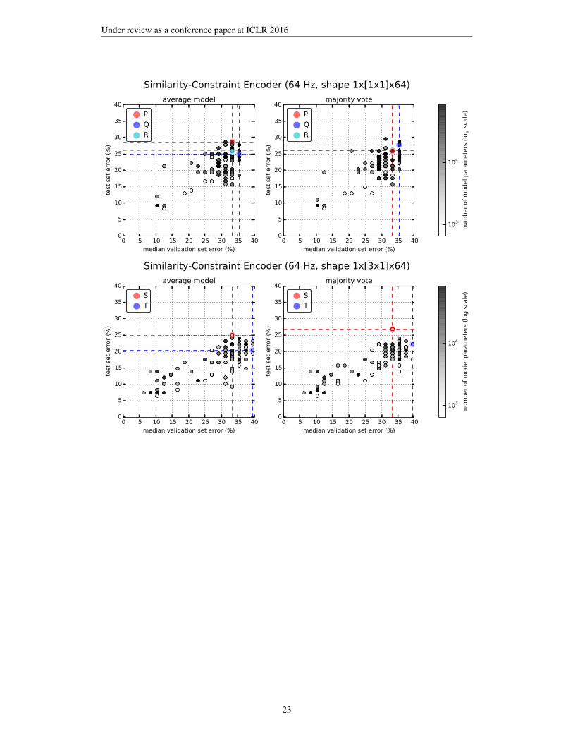
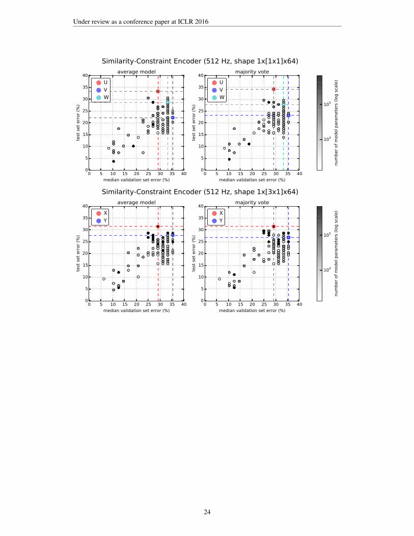
Comparing the baseline classifiers (using raw EEG) with those relying on the learned features aslisted in Table 1 using a z-test, we found a significant improvement at p=0.05 for the SVC modelT. For the average CNN model Y, the improvement over the respective baseline was significant atp=0.061. Both classifiers relied on features learned by similarity-constraint encoding. For the SVCmodels M and Y, we obtained a p-value of 0.068. Due to the rather small test set size (n=108), manyperformance differences were only significant at higher p-values. There appears to be a small per-formance advantage in using the full sampling rate of 512 Hz as indicated by the scatter plots of themodel performance during hyper-parameter optimization shown in Appendix H. Using similarity-constraint encoding to pre-train a simple spatial filter for the first CNN layer that only aggregates the64 EEG channels into a single waveform not only significantly improved the classification accuracybut also reduced the time needed for hyper-parameter optimization from over a week for the fullCNN to a few hours. This improvement makes working at the full sampling rate feasible.

7


In our experiments, we used similarity-constraint encoding to learn global filters. These filters couldbe further adapted to the individual subjects through our hydra-net approach. We believe that thiscombination has a high potential to further improve the pre-trained filters and the resulting classi-fication accuracy. However, technical limitations of our current implementation cause a significantincrease in processing time for this setting (details can be found in Appendix G). We are currentlyworking on a different implementation to resolve this issue.

Amongst the best CNN classifiers, which are listed in Table 3 with more details, models R andW stand out for their simplicity and accuracy that is on par with much bigger models. Their im-provement over the baseline is significant at p=0.1 and p=0.05 respectively. Remarkably, modelR does effectively not even use the second convolutional layer. We interpret this as an indicatorfor the quality of the pre-trained features. Both models are simple enough to allow for interpreta-tion of the learned features by domain experts. Visualizations can be found in Appendix E. Thevisualizations of the layer 1 filters indicate which recording electrodes are most important to theclassifier. The electrodes within the dark red areas that appear bilaterally towards the back of thehead lie directly over the auditory cortex. These electrodes may be picking up on brain activationfrom the auditory cortex that is modulated by the perception of the stimuli. The electrodes withinthe blue areas that appear more centrally may be picking up on the cognitive processes that occur asa result of the brain processing the music at a higher level. In layer 3 there is remarkable similarityof the learned temporal patterns between stimuli 1–4 and their corresponding stimuli 11–14, whichare tempo-matched recordings of songs 1–4 without lyrics (cf. Table 2 for details). This indicatesthat the models have picked up musical features from the stimuli such as down-beats (marking thebeginning of a measure). Further investigations will look at what aspects of the music are causingthese similarities.

Ultimately, we would like to apply the EEG analysis techniques described here in a brain-computerinterface (BCI) setting. To this end, it would be already sufficient to distinguish between two stimuliwith a high accuracy. An analysis of the binary classification performance of model W showedalready promising results with up to perfect accuracy for certain stimulus pairs even though themodel had been only trained for the 12-class problem (cf. Figure 10).

6 CONCLUSIONS

We have proposed several novel techniques for deep feature learning from EEG recordings thataddress specific challenges of this application domain. Cross-trial encoders aim to capture invari-ance between trials within and across subjects. Hydra-nets can learn specifically adapted versionsof selected layers and switch between them based on trial metadata to, for instance, compensatefor differences between subjects. Finally, similarity-constraint encoders allow us to identify signalcomponents that help to distinguish trials of the same class from others. First experiments on theOpenMIIR dataset demonstrate that our techniques are able to learn features that are useful for clas-sification. Most significant improvements over a baseline using raw EEG input were obtained bysimilarity-constraint encoding picking up relevant brain regions as well musically meaningful tem-poral signal characteristics such as the position of down-beats. Furthermore, the learned features arealso still simple enough to allow interpretation by domain experts such as cognitive neuroscientists.

Whilst targeting problems specific to EEG analysis, the proposed techniques are not limited to thiskind of data or even CNNs. Thus, we believe that they will be useful beyond the scope of ourapplication domain. We also hope that this paper will encourage other researchers to join us in thechallenge of decoding brain signals with deep learning techniques. For future work, we want tofurther refine our approach and investigate whether it can be used to identify overlapping featuresbetween music perception and imagery, which would be very useful for BCI settings.

ACKNOWLEDGMENTS

This work has been supported by a fellowship within the Postdoc-Program of the German Aca-demic Exchange Service (DAAD), the Canada Excellence Research Chairs (CERC) Program, anNational Sciences and Engineering Research Council (NSERC) Discovery Grant, an Ontario EarlyResearcher Award, and the James S. McDonnell Foundation. The authors would further like to thankthe study participants.

8


References:

Bergstra, J., Breuleux, O., Bastien, F., Lamblin, P., Pascanu, R., Desjardins, G., Turian, J., Warde-Farley, D.,and Bengio, Y. Theano: a CPU and GPU math expression compiler. In Proc. of the Python for ScientificComputing Conference (SciPy), 2010.

Bourlard, H. and Kamp, Y. Auto-association by multilayer perceptrons and singular value decomposition.Biological Cybernetics, 59(4-5):291–294, 1988.

Cecotti, H. and Graser, A. Convolutional Neural Network with embedded Fourier Transform for EEG classifi-cation. In 19th Int. Conf. on Pattern Recognition (ICPR), pp. 1–4, 2008.

Cecotti, H. and Graser, A. Convolutional Neural Networks for P300 Detection with Application to Brain-Computer Interfaces. IEEE Trans. on Pattern Analysis and Machine Intelligence, 33(3):433–445, 2011.

Fan, R.E., Chang, K.W., Hsieh, C.J., Wang, X.R., and Lin, C.J. Liblinear: A library for large linear classifica-tion. The Journal of Machine Learning Research, 9:1871–1874, 2008.

Glorot, X., Bordes, A., and Bengio, Y. Deep sparse rectifier networks. In NIPS 2010 Workshop on DeepLearning and Unsupervised Feature Learning, 2010.

Goodfellow, I.J., Warde-Farley, D., Lamblin, P., Dumoulin, V., Mirza, M., Pascanu, R., Bergstra, J., Bastien, F.,and Bengio, Y. Pylearn2: a machine learning research library. arXiv: 1308.4214 [cs, stat], 2013.

Goodfellow, I.J., Pouget-Abadie, J., Mirza, M., Xu, B., Warde-Farley, D., Ozair, S., Courville, A., and Bengio,Y. Generative Adversarial Networks. arXiv: 1406.2661 [cs, stat], 2014.

Gramfort, A., Luessi, M., Larson, E., Engemann, D.A., Strohmeier, D., Brodbeck, C., Goj, R., Jas, M., Brooks,T., Parkkonen, L., and Hamalainen, M. MEG and EEG data analysis with MNE-Python. Frontiers inNeuroscience, 7, 2013.

Hinton, G.E., Srivastava, N., Krizhevsky, A., Sutskever, I., and Salakhutdinov, R.R. Improving neural networksby preventing co-adaptation of feature detectors. arXiv:1207.0580, 2012.

Jirayucharoensak, S., Pan-Ngum, S., and Israsena, P. EEG-Based Emotion Recognition Using Deep LearningNetwork with Principal Component Based Covariate Shift Adaptation. The Scientific World Journal, 2014.

Langkvist, M., Karlsson, L., and Loutfi, M. Sleep stage classification using unsupervised feature learning.Advances in Artificial Neural Systems, 2012.

Lee, T., Girolami, M., and Sejnowski, T. J. Independent Component Analysis Using an Extended InfomaxAlgorithm for Mixed Subgaussian and Supergaussian Sources. Neural Computation, 11(2):417–441, 1999.

Masci, J., Meier, U., Ciresan, D., and Schmidhuber, J. Stacked convolutional auto-encoders for hierarchicalfeature extraction. In Proc. of the 21th Int. Conf. on Artificial Neural Networks (ICANN), pp. 52–59, 2011.

Mirowski, P., Madhavan, D., LeCun, Y., and Kuzniecky, R. Classification of patterns of EEG synchronizationfor seizure prediction. Clinical Neurophysiology, 120(11):1927–1940, 2009.

Plis, S.M., Hjelm, D.R., Salakhutdinov, R., Allen, E.A., Bockholt, H.J., Long, J.D., Johnson, H.J., Paulsen,J.S., Turner, J.A., and Calhoun, V.D. Deep learning for neuroimaging: a validation study. Frontiers inNeuroscience, 8, 2014.

Schultz, M. and Joachims, T. Learning a distance metric from relative comparisons. Advances in neuralinformation processing systems (NIPS), pp. 41–48, 2004.

Snoek, J., Larochelle, H., and Adams, R.P. Practical bayesian optimization of machine learning algorithms. InAdvances in Neural Information Processing Systems (NIPS), pp. 2951–2959, 2012.

Stober, S., Cameron, D. J., and Grahn, J. A. Using convolutional neural networks to recognize rhythm stimulifrom electroencephalography recordings. In Advances in Neural Information Processing Systems (NIPS),pp. 1449–1457, 2014a.

Stober, S., Cameron, D.J., and Grahn, J.A. Classifying EEG recordings of rhythm perception. In 15th Int.Society for Music Information Retrieval Conf. (ISMIR), pp. 649–654, 2014b.

Stober, S., Sternin, A, Owen, A.M., and Grahn, J.A. Towards music imagery information retrieval: Introducingthe OpenMIIR dataset of EEG recordings from music perception and imagination. In 16th Int. Society forMusic Information Retrieval Conf. (ISMIR), pp. 763–769, 2015.

Tang, Y. Deep Learning using Linear Support Vector Machines. arXiv: 1306.0239 [cs, stat], 2013.Wang, W., Huang, Y., Wang, Y., and Wang, L. Generalized Autoencoder: A Neural Network Framework

for Dimensionality Reduction. In 2014 IEEE Conference on Computer Vision and Pattern RecognitionWorkshops (CVPRW), pp. 496–503, 2014.

Wulsin, D.F., Gupta, J.R., Mani, R., Blanco, J.A., and Litt, B. Modeling electroencephalography waveformswith semi-supervised deep belief nets: fast classification and anomaly measurement. Journal of NeuralEngineering, 8(3), 2011.

Yang, Y. and Shah, M. Learning discriminative features and metrics for measuring action similarity. In 2014IEEE International Conference on Image Processing (ICIP), pp. 1555–1559, 2014.

Zheng, W.-L., Zhu, J.-Y., Peng, Y., and Lu, B.-L. EEG-based emotion classification using deep belief networks.In 2014 IEEE Int. Conf. on Multimedia and Expo (ICME), pp. 1–6, 2014.

9


A ADDITIONAL INFORMATION ABOUT THE OPENMIIR MUSIC STIMULI

Table 2: Information about the tempo, meter and length of the stimuli (without cue clicks).ID Name Meter Length Tempo

1 Chim Chim Cheree (lyrics) 3/4 13.3s 212 BPM2 Take Me Out to the Ballgame (lyrics) 3/4 7.7s 189 BPM3 Jingle Bells (lyrics) 4/4 9.7s 200 BPM4 Mary Had a Little Lamb (lyrics) 4/4 11.6s 160 BPM

11 Chim Chim Cheree 3/4 13.5s 212 BPM12 Take Me Out to the Ballgame 3/4 7.7s 189 BPM13 Jingle Bells 4/4 9.0s 200 BPM14 Mary Had a Little Lamb 4/4 12.2s 160 BPM21 Emperor Waltz 3/4 8.3s 178 BPM22 Hedwig’s Theme (Harry Potter) 3/4 16.0s 166 BPM23 Imperial March (Star Wars Theme) 4/4 9.2s 104 BPM24 Eine Kleine Nachtmusik 4/4 6.9s 140 BPM

mean 10.4s 176 BPM

10


B VISUALIZATIONS OF COMMON COMPONENTS

Figure 3: Topographic map visualization of the EEG channel weights for the top-4 signal compo-nents derived from the perception trials. The leftmost two columns show the top-4 principal compo-nents (explaining over 80% of the variance in total; individual values are shown next to the compo-nents) and the corresponding independent components computed using extended Infomax ICA. Theremaining columns show the weights learned by a tied-weights convolutional auto-encoder for allsubjects combined (third column) and all individual subjects labeled P01 to P14 accordingly using4 filters of width 1 (samples) with tanh nonlinearity and without biases. Noisy EEG channels thatwere removed and interpolated are marked by red X’s. Values at the bottom of each column refer tothe mean squared reconstruction error (MRSE) per sample, which was used as cost function.

Figure 4: Topographic map visualization of the EEG channel weights for the top-4 signal compo-nents derived from the cued imagination trials. They look very similar to the ones shown in Figure 3for the perception trials. The leftmost two columns show the top-4 principal components (explainingover 80% of the variance in total; individual values are shown next to the components) and the corre-sponding independent components computed using extended Infomax ICA. The remaining columnsshow the weights learned by a tied-weights convolutional auto-encoder for all subjects combined(third column) and all individual subjects labeled P01 to P14 accordingly using 4 filters of width 1(samples) with tanh nonlinearity and without biases. Noisy EEG channels that were removed andinterpolated are marked by red X’s. Values at the bottom of each column refer to the mean squaredreconstruction error (MRSE) per sample, which was used as cost function.

11


C FURTHER VISUALIZATIONS OF CROSS-TRIAL ENCODERS

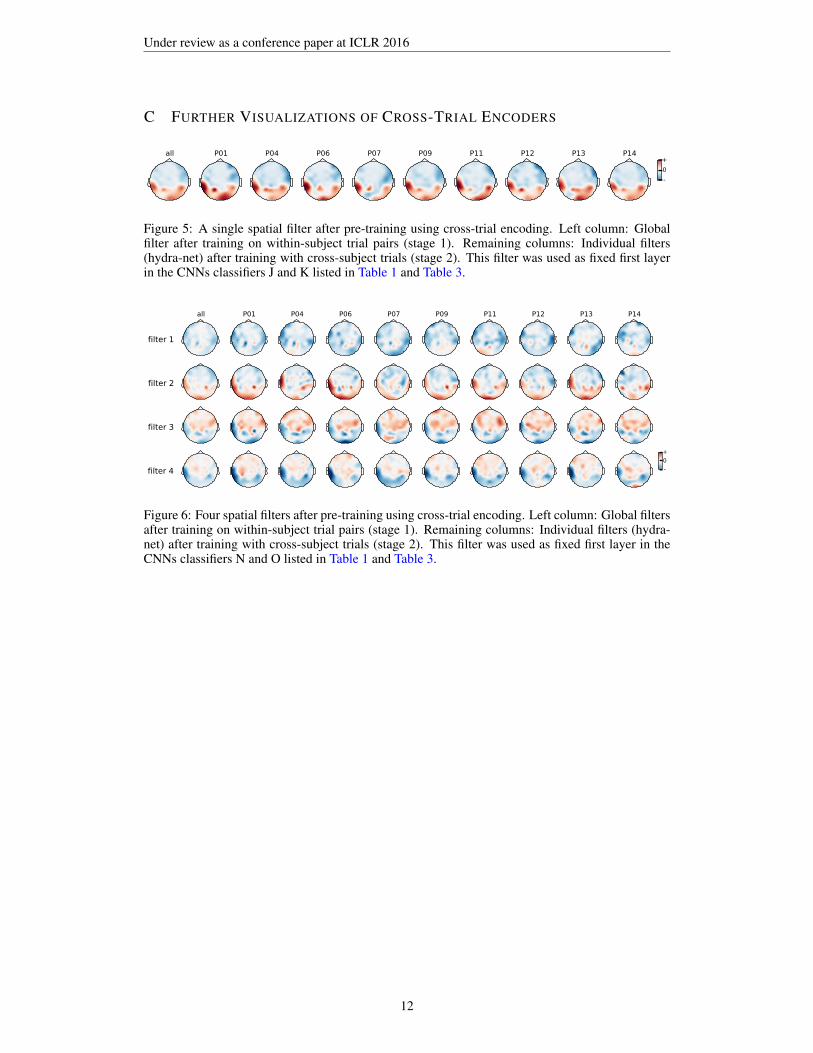
Figure 5: A single spatial filter after pre-training using cross-trial encoding. Left column: Globalfilter after training on within-subject trial pairs (stage 1). Remaining columns: Individual filters(hydra-net) after training with cross-subject trials (stage 2). This filter was used as fixed first layerin the CNNs classifiers J and K listed in Table 1 and Table 3.

Figure 6: Four spatial filters after pre-training using cross-trial encoding. Left column: Global filtersafter training on within-subject trial pairs (stage 1). Remaining columns: Individual filters (hydra-net) after training with cross-subject trials (stage 2). This filter was used as fixed first layer in theCNNs classifiers N and O listed in Table 1 and Table 3.

12


D DETAILED CNN CLASSIFIER PERFORMANCE

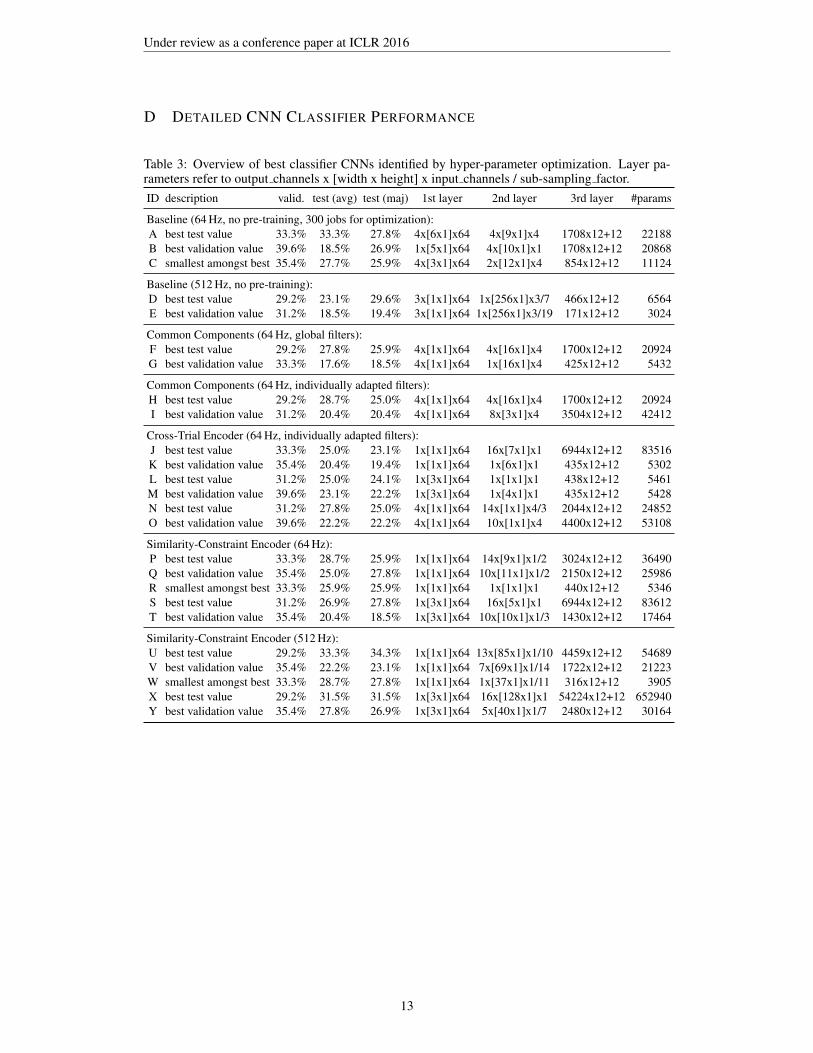
Table 3: Overview of best classifier CNNs identified by hyper-parameter optimization. Layer pa-rameters refer to output channels x [width x height] x input channels / sub-sampling factor.ID description valid. test (avg) test (maj) 1st layer 2nd layer 3rd layer #params

Baseline (64 Hz, no pre-training, 300 jobs for optimization):A best test value 33.3% 33.3% 27.8% 4x[6x1]x64 4x[9x1]x4 1708x12+12 22188B best validation value 39.6% 18.5% 26.9% 1x[5x1]x64 4x[10x1]x1 1708x12+12 20868C smallest amongst best 35.4% 27.7% 25.9% 4x[3x1]x64 2x[12x1]x4 854x12+12 11124

Baseline (512 Hz, no pre-training):D best test value 29.2% 23.1% 29.6% 3x[1x1]x64 1x[256x1]x3/7 466x12+12 6564E best validation value 31.2% 18.5% 19.4% 3x[1x1]x64 1x[256x1]x3/19 171x12+12 3024

Common Components (64 Hz, global filters):F best test value 29.2% 27.8% 25.9% 4x[1x1]x64 4x[16x1]x4 1700x12+12 20924G best validation value 33.3% 17.6% 18.5% 4x[1x1]x64 1x[16x1]x4 425x12+12 5432

Common Components (64 Hz, individually adapted filters):H best test value 29.2% 28.7% 25.0% 4x[1x1]x64 4x[16x1]x4 1700x12+12 20924I best validation value 31.2% 20.4% 20.4% 4x[1x1]x64 8x[3x1]x4 3504x12+12 42412

Cross-Trial Encoder (64 Hz, individually adapted filters):J best test value 33.3% 25.0% 23.1% 1x[1x1]x64 16x[7x1]x1 6944x12+12 83516K best validation value 35.4% 20.4% 19.4% 1x[1x1]x64 1x[6x1]x1 435x12+12 5302L best test value 31.2% 25.0% 24.1% 1x[3x1]x64 1x[1x1]x1 438x12+12 5461M best validation value 39.6% 23.1% 22.2% 1x[3x1]x64 1x[4x1]x1 435x12+12 5428N best test value 31.2% 27.8% 25.0% 4x[1x1]x64 14x[1x1]x4/3 2044x12+12 24852O best validation value 39.6% 22.2% 22.2% 4x[1x1]x64 10x[1x1]x4 4400x12+12 53108

Similarity-Constraint Encoder (64 Hz):P best test value 33.3% 28.7% 25.9% 1x[1x1]x64 14x[9x1]x1/2 3024x12+12 36490Q best validation value 35.4% 25.0% 27.8% 1x[1x1]x64 10x[11x1]x1/2 2150x12+12 25986R smallest amongst best 33.3% 25.9% 25.9% 1x[1x1]x64 1x[1x1]x1 440x12+12 5346S best test value 31.2% 26.9% 27.8% 1x[3x1]x64 16x[5x1]x1 6944x12+12 83612T best validation value 35.4% 20.4% 18.5% 1x[3x1]x64 10x[10x1]x1/3 1430x12+12 17464

Similarity-Constraint Encoder (512 Hz):U best test value 29.2% 33.3% 34.3% 1x[1x1]x64 13x[85x1]x1/10 4459x12+12 54689V best validation value 35.4% 22.2% 23.1% 1x[1x1]x64 7x[69x1]x1/14 1722x12+12 21223W smallest amongst best 33.3% 28.7% 27.8% 1x[1x1]x64 1x[37x1]x1/11 316x12+12 3905X best test value 29.2% 31.5% 31.5% 1x[3x1]x64 16x[128x1]x1 54224x12+12 652940Y best validation value 35.4% 27.8% 26.9% 1x[3x1]x64 5x[40x1]x1/7 2480x12+12 30164

13


E MODEL VISUALIZATIONS

Layer

3 (

class

es)

Layer 1

-

0

+

Layer 2

123411121314212223

0 100 200 300 400

time (in samples)

24

Figure 7: Visualization of CNN R (average of the 9 cross-validation fold models), which processesraw EEG at a sampling rate of 64 Hz. Layer 1 was pre-trained using similarity-constraint encoding.

Layer

3 (

class

es)

Layer 1

-

0

+

0 5 10 15 20 25 30 35Layer 2

123411121314212223

0 50 100 150 200 250 300

time (in samples, down-sampled by factor 11)

24

Figure 8: Visualization of CNN W (average of the 9 cross-validation fold models), which processesraw EEG at a sampling rate of 512 Hz. Layer 1 was pre-trained using similarity-constraint encoding.

14


F CONFUSION ANALYSIS FOR CNN MODEL W (AVG)12-Class Stimuli Confusion

2015-12-01 Sebastian Stober - Deep Feature Learning for EEG 51

Chim Chim Cheree (lyrics) Take Me Out to the Ballgame (lyrics)

Jingle Bells (lyrics) Mary Had a Little Lamb (lyrics)

Chim Chim Cheree Take Me Out to the Ballgame

Jingle Bells Mary Had a Little Lamb

Emperor Waltz Hedwig’s Theme (Harry Potter)

Imperial March (Star Wars Theme) Eine Kleine Nachtmusik

Figure 9: 12-class confusion matrix for CNN W (average of the 9 cross-validation fold models).

1

2

2

3

3

4

4

11

11

12

12

13

13

14

14

21

21

22

22

23

23

242 3 4 11 12 13 14 21 22 23 24

Stimulus Class B

1

2

3

4

11

12

13

14

21

22

23

Sti

mulu

s C

lass

A

Stimulus Class B

Stim

ulu

s Cla

ss Abinomial p-value

0.05

0.010.005

0.0010.0005

0.00015e-05

Figure 10: Binary confusion matrices for CNN W (average of the 9 cross-validation fold models).For each binary classification, only the 18 test trials belonging to either stimulus class A or stimulusclass B were considered. The inset at the lower bottom visualizes the p-values determined by usingthe cumulative binomial distribution to estimate the likelihood of observing the resepective binaryclassification rate by chance. Note that the classifier was only trained for the 12-class problem.

15


G IMPLEMENTATION DETAILS

For reproducibility and to encourage further developments and research in this direction, all code necessary tobuild the proposed deep network structures and to run the experiments described in the following is shared asopen source within the deepthought library.11 The implementation is based on the libraries Pylearn2 (Goodfel-low et al. (2013)) and Theano (Bergstra et al. (2010)) and comprises various custom Layer and Dataset classes– such as for on-the-fly generation of trial tuples and the respective classification targets during iteration.

The following subsections provide details about our implementation.

G.1 DETAILS ON CONVOLUTIONAL AUTO-ENCODERS FOR EEG

Convolutional autoencoders are a special variant of CNNs that encode their input using convolution into acompressed internal representation which is then decoded using de-convolution into the original space trying tominimize the reconstruction error. Such encoder/decoder pairs can optionally be stacked as described in Masciet al. (2011) to increase the complexity of the internal representations.

We considered two measures of the reconstruction quality. The mean square reconstruction error (MSRE) is thecommonly used error measure for auto-encoding and computed as the squared Euclidean distance between theinput and the reconstruction averaged over all samples. We further define the mean channel correlation (MCC)as the mean correlation of the individual input channels and their reconstructions. The correlation is computedas Pearson’s r, which is in the range [-1,1] where 1 is total positive correlation, 0 is no correlation, and -1 istotal negative correlation.

The convolutional filters applied on multi-channel raw EEG data are 2-dimensional where the width is time(samples) and the height is optionally used for different frequency bands in a time-frequency representation,which is not considered in the context of this paper. In the simplest case, the filter width in the time dimension isonly 1. A CNNs with k filters then behaves like a conventional feed-forward network without convolution thataggregates EEG data for a single time point across all channels into k output values – with the only differencethat the CNN processes the whole recording as one input.

Such a convolutional auto-encoder with filter width 1 and linear activation functions is strongly related to PCA(Bourlard & Kamp (1988)) and consequently obtains similar results. Using an auto-encoder, however, opensup further possibilities such as non-linear activation functions, a filter width greater than 1, regularization ofchannel weights and activations, and stacking multiple encoder/decoder layer pairs. This allows to identifymore complex components, which can also cover the time dimension.

Here, we used all training trials from the dataset for training which were preprocessed as described in Section 3.The training trials have different lengths due to the different duration of the stimuli. As the network expectsinputs of equal length, shorter trials were zero-padded at the end to match the duration of the longest stimulus.12

Zero-padded trials should not be used for supervised training because this will result in the trial length beingused as a distinctive feature, which is not desirable. However, for unsupervised pre-training using basic auto-encoding, the variable trial length is not problematic as the objective here is only to reconstruct.

The de-convolution filters were set to share the weights with the corresponding convolution filters. We experi-mented with different activation functions – linear, tanh and rectified linear (Glorot et al. (2010)) – and obtainedvery similar topographies that only had small variations in intensity. We finally selected the tanh nonlinearitybecause its output matches the value range of the network inputs ([-1,1]). Furthermore, we found that usingbias terms did not lead to improvements and therefore chose network units without bias.

Comparing the commonly used MSRE to the MCC measure showed that MSRE was the superior cost functionin this setting. The training process was generally very stable such that a high learning rate with linear decayover epochs in combination with momentum could be used to quickly obtain results. As termination criterion,we tracked the error on the training set for early stopping and specified a (rather defensive) maximum of 1000epochs.

We first trained an auto-encoder for all trials of the perception condition. The learned filter weights werethen used as initialization values for individual auto-encoders for each subject. Minor differences betweensubjects can be recognized in the example shown in Figure 3 but the component relations between subjectsare still obvious. This was generally the case for different network structures that we tested. The individualcomponents seem to be very stable. For instance, the results obtained with the same network on the imaginationtrials with cue (condition 2; otherwise not considered in the context of this paper) only differ slightly as shownin Figure 4.

11https://github.com/sstober/deepthought (code will be updated paper publication)12This is a limitation of our current Pylearn2-based implementation. In principle, convolutional auto-

encoders can operate on variable-length input.

16

https://github.com/sstober/deepthought


G.2 IMPLEMENTING A HYDRA-NET

Hydra-nets allow to have separate processing pathways for subsets of a dataset – such as all trials of the samesubject or all trials belonging to the same stimulus. We call the respective meta-data property that controls thechoice of the individual pathway the selector. The selector data needs to be provided additionally to the regularnetwork input and, if necessary, has to be propagated (without being processed) up to the point where it is usedto choose the individual processing pathway. Individualization can range from a single layer with differentweights for each value of the selector up to multi-layer sub-networks that may also differ in their structure aslong as their input and output format is identical.

In our implementation, we wrapped the part of the network that we wanted to individualize with a hydra-netlayer. Within this wrapper layer, a copy of the internal network was created for each possible selector value. Foreach input, the respective individualized version of the internal network was chosen based on the additionallyprovided selector input. For mini-batch processing, we implemented two different strategies:

a) Compute the output of all individual pathways and apply a mask based on the selector values for thewhole mini-batch.

b) Iterate through the input instances within the mini-batch (using Theano’s scan operation) and processeach one individually solely with the selected individual pathway. (For selection, Theano’s ifelseoperation was used that implements a lazy evaluation.)

Option a) is highly inefficient as it results in an overhead of unnecessary computations. This effect gets worsewith an increasing number of different selector values. For option b), this is not the case. However, there is adifferent performance penalty from using the scan function. In the experiments described in Section 4.3, wefound that option a) still performed slightly better. We plan to optimize our code and investigate different waysto implement hydra-net layers for future experiments.

G.3 TRAINING A CROSS-TRIAL ENCODER WITH CROSS-SUBJECT TRIAL PAIRS

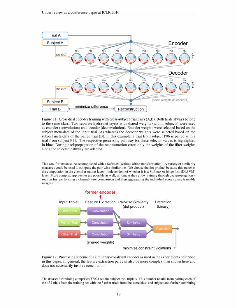
Figure 11 shows the network structure of the auto-encoder that learned the spatial filters shown in Figure 5.Here, we used two separate hydra-net layers – one as encoder and the other one as decoder. Both shared theirweights, i.e., for the same subject, the convolution and deconvolution filter would be identical. The encoderhydra-net layer used the subject of the input trial as selector (subject A) whereas the decoder hydra-net layerused the subject of the paired trial (subject B). This general structure was identical for all cross-trial encodersconsidered here except for the shape and number of the filters used.

For initialization, we first trained a basic auto-encoder on all 1296 (= 432x3) within-subject trial pairs derivedfrom the training set. This way, we obtained the general filters labeled “all” in Figures 1, 5 and 6. We thencontinued trained a copy of the general cross-trial encoder for each individual subject. Finally, we used theresulting individual filters as initialization for the hydra-net. This network was trained on 15120 (= 432x(4x9- 1)) cross-subject trial pairs. In order to avoid excessive memory usage of the dataset, we implemented adataset wrapper that only stored an index data structure and generated mini-batches of paired trials and selectormeta-data on-the-fly from a base dataset when they were requested.

G.4 CONSTRUCTING AND TRAINING A SIMILARITY-CONSTRAINT ENCODER

Starting from a basic auto-encoder, a similarity-constraint encoder as shown schematically in Figure 12 canbe constructed as follows: The decoder part of the original auto-encoder can be removed as we are now onlyinterested in the internal feature representations and their similarity.13 Next, we redesign the encoder part suchthat it can process multiple trials at the same time as a single input tuple. To ensure that all trials within a tupleare processed in the exactly same way, weights and biases need to be shared between the parallel processingpipelines. One easy way to achieve such a weight sharing for basic CNN-based architectures is by adding a thirddimension for the trials (additionally to the channels and time/samples axes) and using filters of size 1 along thisdimension. Unfortunately, this approach of convolution along the trials axis does not work together with hydra-net layers. Here, different individualized weights for the different trials of the input tuple might be requiredwithin the processing pipeline. In our implementation, we therefore wrap the processing pipeline within acustom layer that takes care of processing each trial separately (using individualized weights if necessary) andthen computes the pair-wise similarities between the reference trial and the other trials. For k-tuples, thisresults in k − 1 similarity scores. The final output layer only has to predict the trial with the highest value.

13Note that simply maximizing the feature similarity for the paired trials used for cross-trial encoding wouldbe an ill-posed learning problem. The optimum could easily be achieved by transforming all inputs into thesame representation. This way, all trials would have maximum similarity – including those from differentclasses. It would also be impractical to train the network with pre-defined target similarity values for all possiblepairs of trials.

17


Trial B

Subject A

Subject B

Reconstruction

Encoder

Decoder

select

select

Trial A

minimize difference

(same weights as encoder)

Figure 11: Cross-trial encoder training with cross-subject trial pairs (A,B). Both trials always belongto the same class. Two separate hydra-net layers with shared weights (within subjects) were usedas encoder (convolution) and decoder (deconvolution). Encoder weights were selected based on thesubject meta-data of the input trial (A) whereas the decoder weights were selected based on thesubject meta-data of the paired trial (B). In this example, a trial from subject P06 is paired with atrial from subject P11. The respective processing pathway for these selector values is highlightedin blue. During backpropagation of the reconstruction error, only the weights of the filter weightsalong the selected pathway are adapted.

This can, for instance, be accomplished with a Softmax (without affine transformation). A variety of similaritymeasures could be used to compute the pair-wise similarities. We choose the dot product because this matchesthe computation in the classifier output layer – independent of whether it is a Softmax or hinge loss (DLSVM)layer. More complex approaches are possible as well, as long as they allow training through backpropagation –such as first performing a channel-wise comparison and then aggregating the individual scores using trainableweights.

minimize constraint violations

Deconvolution Output Input

Input

Input

Reference

Paired Trial

Other Trial

Convolution

Convolution

Feature Extraction

Similarity-Constraint Encoder

2015-12-01 Sebastian Stober - Deep Feature Learning for EEG 46

Input Triplet

(virtual network structure)

(shared weights)

Pairwise Similarity (dot product)

Prediction (binary)

former encoder

Similarity

Similarity

Convolution

Classifier

Figure 12: Processing scheme of a similarity-constraint encoder as used in the experiments describedin this paper. In general, the feature extraction part can also be more complex than shown here anddoes not necessarily involve convolution.

The dataset for training comprised 57024 within-subject trial triplets. This number results from pairing each ofthe 432 trials from the training set with the 3 other trials from the same class and subject and further combining

18


these pairs with the 11x4 trials from the same subject that belong to a different class. As for cross-trial encodertraining, we again implemented a dataset wrapper that only requires storing an index data structure for thetuples from a base dataset.

G.5 SIMILARITY-CONSTRAINT ENCODERS WITH HYDRA-NET LAYERS

We believe that the combination of similarity-constraint encoding with the hydra-net approach to account forindividual differences between subjects has a high potential to further improve pre-trained global filters andthe resulting classification accuracy. An experiment with synthesized data has already shown the feasibilityof this combined approach. For this test, we generated random single-channel signals for 12 stimuli. Thesesignals were then added to 64-channel Gaussian noise, randomly choosing a different channel for each subjectto contain the relevant signal. As in our real dataset, we had 9 different subjects. Using these synthetic data,a basic similarity-constraint encoder was able to identify the combined set of channels that contained relevantsignals for the group of all subject. Turning the first layer into a hydra-net layer allowed the spatial filters tobecome more specific and the network correctly learned the individual channel masks.

Training on the real dataset with less defined signals and much more structured background noise is of coursemuch harder. However, the biggest obstacle is currently the increase in processing time caused by the addedcomputational complexity of the hydra-net layer (cf. Section G.2) with the amount of triplets available fortraining. From the training set of 432 trials, 57024 within-subject trial triplets can be derived as describedearlier. Considering also cross-subject trial triplets increases the number to 5987520 (= 432x(4x9-1)x(11x4x9)).Using training sets of this size is still feasible. However, the hydra-net processing overhead should be addressedbefore attempting this.

19


H CLASSIFIER PERFORMANCE DURING HYPER-PARAMETER OPTIMIZATION

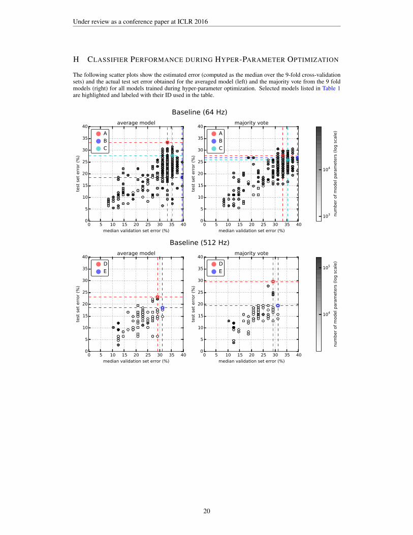
The following scatter plots show the estimated error (computed as the median over the 9-fold cross-validationsets) and the actual test set error obtained for the averaged model (left) and the majority vote from the 9 foldmodels (right) for all models trained during hyper-parameter optimization. Selected models listed in Table 1are highlighted and labeled with their ID used in the table.

0 5 10 15 20 25 30 35 40

median validation set error (%)

0

5

10

15

20

25

30

35

40

test

set

err

or

(%)

average model

A

B

C

0 5 10 15 20 25 30 35 40


0

5

10

15

20

25

30

35

40

test

set

err

or

(%)

majority vote

A

B

C

103

104

num

ber

of

model para

mete

rs (

log s

cale

)

Baseline (64 Hz)

0 5 10 15 20 25 30 35 40


0

5

10

15

20

25

30

35

40

test

set

err

or

(%)

average model

D

E

0 5 10 15 20 25 30 35 40


0

5

10

15

20

25

30

35

40

test

set

err

or

(%)

majority vote

D

E

104

105

num

ber

of

model para

mete

rs (

log s

cale

)

Baseline (512 Hz)

20


0 5 10 15 20 25 30 35 40


0

5

10

15

20

25

30

35

40te

st s

et

err

or

(%)

average model

F

G

0 5 10 15 20 25 30 35 40


0

5

10

15

20

25

30

35

40

test

set

err

or

(%)

majority vote

F

G

103

104

num

ber

of

model para

mete

rs (

log s

cale

)

Common Components (64 Hz, global filters)

0 5 10 15 20 25 30 35 40


0

5

10

15

20

25

30

35

40

test

set

err

or

(%)

average model

H

I

0 5 10 15 20 25 30 35 40


0

5

10

15

20

25

30

35

40

test

set

err

or

(%)

majority vote

H

I

103

104

num

ber

of

model para

mete

rs (

log s

cale

)

Common Components (64 Hz, individually adapted filters)

21


0 5 10 15 20 25 30 35 40


0

5

10

15

20

25

30

35

40te

st s

et

err

or

(%)

average model

J

K

0 5 10 15 20 25 30 35 40


0

5

10

15

20

25

30

35

40

test

set

err

or

(%)

majority vote

J

K

103

104

num

ber

of

model para

mete

rs (

log s

cale

)

Cross-Trial Encoder (64 Hz, individually adapted filters, shape 1x[1x1]x64)

0 5 10 15 20 25 30 35 40


0

5

10

15

20

25

30

35

40

test

set

err

or

(%)

average model

L

M

0 5 10 15 20 25 30 35 40


0

5

10

15

20

25

30

35

40

test

set

err

or

(%)

majority vote

L

M

103

104

num

ber

of

model para

mete

rs (

log s

cale

)


0 5 10 15 20 25 30 35 40


0

5

10

15

20

25

30

35

40

test

set

err

or

(%)

average model

N

O

0 5 10 15 20 25 30 35 40


0

5

10

15

20

25

30

35

40

test

set

err

or

(%)

majority vote

N

O

103

104

num

ber

of

model para

mete

rs (

log s

cale

)


22


0 5 10 15 20 25 30 35 40


0

5

10

15

20

25

30

35

40te

st s

et

err

or

(%)

average model

P

Q

R

0 5 10 15 20 25 30 35 40


0

5

10

15

20

25

30

35

40

test

set

err

or

(%)

majority vote

P

Q

R

103

104

num

ber

of

model para

mete

rs (

log s

cale

)

Similarity-Constraint Encoder (64 Hz, shape 1x[1x1]x64)

0 5 10 15 20 25 30 35 40


0

5

10

15

20

25

30

35

40

test

set

err

or

(%)

average model

S

T

0 5 10 15 20 25 30 35 40


0

5

10

15

20

25

30

35

40

test

set

err

or

(%)

majority vote

S

T

103

104

num

ber

of

model para

mete

rs (

log s

cale

)


23


0 5 10 15 20 25 30 35 40


0

5

10

15

20

25

30

35

40te

st s

et

err

or

(%)

average model

U

V

W

0 5 10 15 20 25 30 35 40


0

5

10

15

20

25

30

35

40

test

set

err

or

(%)

majority vote

U

V

W

104

105

num

ber

of

model para

mete

rs (

log s

cale

)


0 5 10 15 20 25 30 35 40


0

5

10

15

20

25

30

35

40

test

set

err

or

(%)

average model

X

Y

0 5 10 15 20 25 30 35 40


0

5

10

15

20

25

30

35

40

test

set

err

or

(%)

majority vote

X

Y

104

105

num

ber

of

model para

mete

rs (

log s

cale

)


24

deep feature learning for eeg recordings - arxiv · izontal and vertical electrooculography (eog)...

Documents