Deep CNN for Segmentation of Myocardial ASL Short-Axis Data:

Accuracy, Uncertainty, and Adaptability

Hung P. Do1, Yi Guo2, Andrew J. Yoon3, and Krishna S. Nayak4

1Canon Medical Systems USA, Inc.

2Snap Inc.

3Long Beach Memorial Medical Center, University of California Irvine

4University of Southern California

ISMRM Workshop on Machine Learning, Washington DC, Oct 26-28, 2018

Speaker Name: Hung Do

Company Name: Canon Medical Systems USA, Inc. (formerly Toshiba Medical)

Type of Relationship: Employee

Declaration of

Financial Interests or Relationships

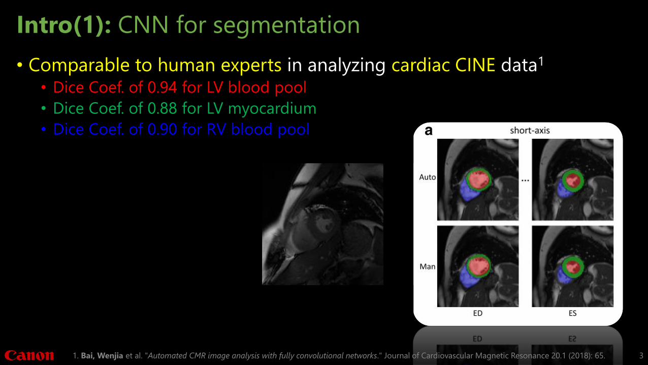
Intro(1): CNN for segmentation

• Comparable to human experts in analyzing cardiac CINE data1

• Dice Coef. of 0.94 for LV blood pool

• Dice Coef. of 0.88 for LV myocardium

• Dice Coef. of 0.90 for RV blood pool

1. Bai, Wenjia et al. "Automated CMR image analysis with fully convolutional networks." Journal of Cardiovascular Magnetic Resonance 20.1 (2018): 65. 3

Goals

1. To apply CNN for segmentation of myocardial Arterial Spin Labeled (ASL) data

2. To measure model uncertainty using Monte Carlo dropout

3. To adapt the CNN model to the desired trade-off between false positive (FP) and false negative (FN) using Tversky loss function

4

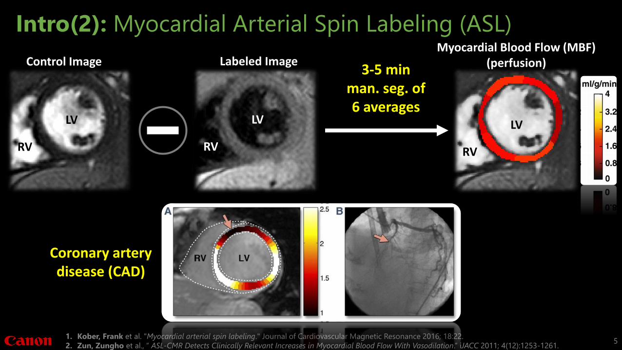
Intro(2): Myocardial Arterial Spin Labeling (ASL)

1. Kober, Frank et al. "Myocardial arterial spin labeling." Journal of Cardiovascular Magnetic Resonance 2016; 18:22.

2. Zun, Zungho et al., “ ASL-CMR Detects Clinically Relevant Increases in Myocardial Blood Flow With Vasodilation.” iJACC 2011; 4(12):1253-1261.5

3-5 minman. seg. of6 averages

Coronary artery disease (CAD)

Control Image

LV

RV

Labeled Image

LV

RV

Myocardial Blood Flow (MBF)(perfusion)

LV

RV

Intro(3): Characteristics of ASL data

• Low resolution

• Low SNR and CNR

• Varying SNR and CNR

6

LV

RV

Labeled images Control images

CINE images

Intro(4): Partial volume effects

• Ventricular blood and epicardial fat have different physical properties and spin history compared to myocardium.

1. Wikimedia Commons contributors, "File:Heart normal short axis section.jpg," Wikimedia Commons, the free media repository, (accessed October 11, 2018). 7

LVRV LV

RVFat

Fat

Myocardium

Myocardium

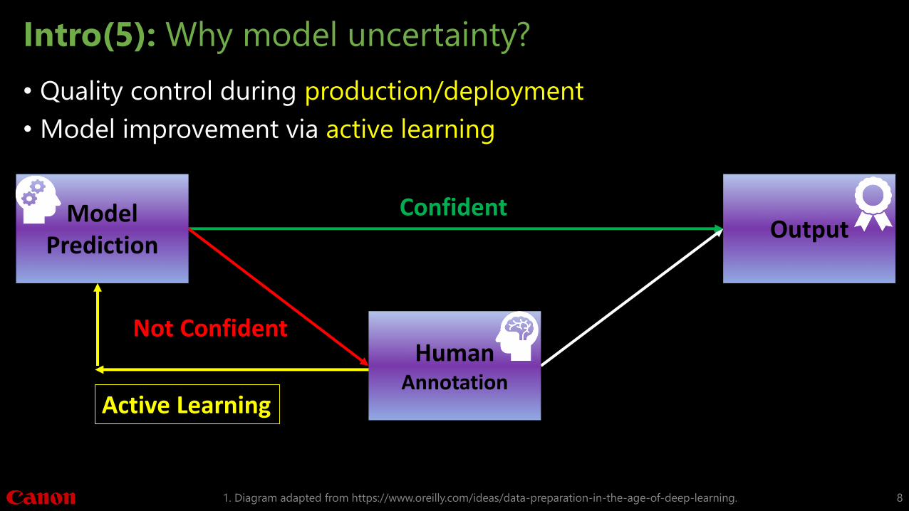
Intro(5): Why model uncertainty?

• Quality control during production/deployment

• Model improvement via active learning

1. Diagram adapted from https://www.oreilly.com/ideas/data-preparation-in-the-age-of-deep-learning. 8

HumanAnnotation

Active Learning

Confident

Not Confident

Model Prediction

Output

Methods(1): Network Architecture1

5x5 Conv+ReLU+BN 1x1 Conv+Sigmoid

C Channel Concatenation

Max Pooling UpsamplingMonte Carlo Dropout

C

C

C

CInput

Output

1. Ronneberger O et al., "U-net: Convolutional networks for biomedical image segmentation." 2015; arXiv:1505.04597. 9

loss = Binary Cross-Entropy or (1 – Soft-Dice) or (1 – Tversky Index)

Methods(2): Dataset and training parameters

• Training and validation data1:• From 22 subjects: 478 images – 438/40 images for training/validation

• Test data1:• From 6 “un-seen” heart transplant patients: 144 images (rest and during

Adenosine stress)

• Training parameters:• 150 epochs

• Learning rate: 1e-4

• Dropout rate: 0.5

• Batch size = 12

• Adam optimizer

1. Do, Hung et al, “Double-gated Myocardial ASL Perfusion Imaging is Robust to Heart Rate Variation.” Magn Reson Med 2017; 77(5):1975-1980. 10

Methods(4): Adaptability using Tversky loss

1. Tversky, Amos. "Features of similarity." Psychological Review 1977;84(4): 327-52.

2. Wikipedia contributors. "Jaccard index." Wikipedia, The Free Encyclopedia. Wikipedia, The Free Encyclopedia, 20 Sep. 2018. Web. 5 Oct. 2018.11

𝑫𝒊𝒄𝒆 =𝟐⋅|𝑨 ⋂𝑩|

𝑨 +|𝑩|

𝑫𝒊𝒄𝒆 =𝟐⋅𝑻𝑷

𝟐⋅𝑻𝑷+𝑭𝑷+𝑭𝑵=

𝑻𝑷

𝑻𝑷+𝟎.𝟓⋅𝑭𝑷+𝟎.𝟓⋅𝑭𝑵TPFP FN

Tversky loss = 1- Tversky Index1

𝑻𝒗𝒆𝒓𝒔𝒌𝒚 𝑰𝒏𝒅𝒆𝒙 =𝑻𝑷

𝑻𝑷 + (𝟏 − β) ⋅ 𝑭𝑷 + β ⋅ 𝑭𝑵

A: Predicted MaskB: Reference Mask

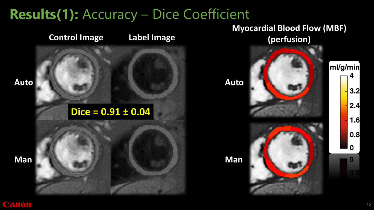
Results(1): Accuracy – Dice Coefficient

12

Auto

Man

Auto

Man

Myocardial Blood Flow (MBF)(perfusion)Control Image Label Image

Dice = 0.91 ± 0.04

Results(1): Accuracy – Myocardial Blood Flow (MBF)

13

y = 0.9877x + 0.0244R² = 0.9613

-2

0

2

4

6

8

10

-2 0 2 4 6 8 10

AU

TO S

EGM

ENTA

TIO

NMANUAL SEGMENTATION

Regional MBF (ml/g/min)

MBF measured using automatic segmentation is highly correlated to that measured using manual segmentation

Results(2): Uncertainty

14

y = 5.4434x + 0.0641R² = 0.637

0.05

0.1

0.15

0.2

0.25

0.3

0.0025 0.0075 0.0125 0.0175 0.0225 0.0275

NO

RM

ALI

ZED

MC

STD

DICE STD

Normalized MC STD vs. Dice STD

MC STD

Without manual segmentation

Given man. segmentation

Dice STD

1115 MC trials

y = 5.4434x + 0.0641R² = 0.637

0.05

0.1

0.15

0.2

0.25

0.3

0.0025 0.0075 0.0125 0.0175 0.0225 0.0275

NO

RM

ALI

ZED

MC

STD

DICE STD

Normalized MC STD vs. Dice STD

Auto: Dashed lines Man: White solid lines

Results(2): Uncertainty

15

MC STDMC STD

1115 MC trials

0.229 0.367 0.744 1.49 2.716

12

24

0

5

10

15

20

25

16 32 64 128 256 512 1024 2048INFE

REN

CE

TIM

E (S

ECO

ND

)

NUMBER OF MC TRIALS

Inference Time vs. # of MC trials

0

0.005

0.01

0.015

0.02

0.025

0.03

16 32 64 128 256 512 1024 2048

UN

CER

TAIN

TY

NUMBER OF MC TRIAL

Model Uncertainty

Results(2): Uncertainty – Time penalty per image

16

Batch Size = 64

~1.5s/image with 128 MC trials

Results(3): Adaptability – Partial volume effects

17

y = 1.0166x - 0.1445R² = 0.9523

-2

0

2

4

6

8

10

-2 0 2 4 6 8 10

THIN

SEG

MEN

TATI

ON

ORIGNIGAL SEGMENTATION

Regional MBF: Thin vs. Orig.

y = 0.9811x + 1.1951R² = 0.8266

-2

0

2

4

6

8

10

-2 0 2 4 6 8 10

THIC

K S

EGM

ENTA

TIO

N

ORIGNIGAL SEGMENTATION

Regional MBF: Thick vs. Orig.

Dice = 0.80 ± 0.04 Dice = 0.81 ± 0.02

FP = 0FN ~300 pixels/im

FP ~400 pixels/imFN = 0

Original/ManThin mask Thick mask

Significant overestimation due to partial volume effects

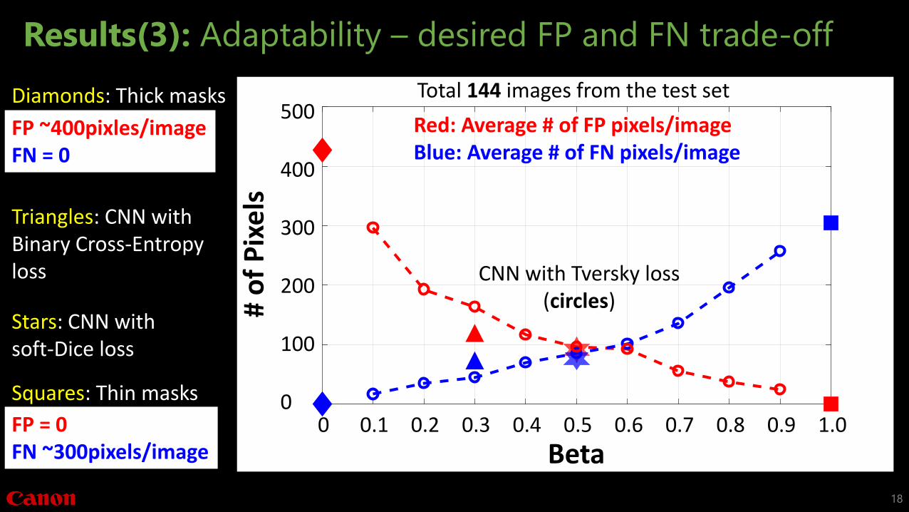
Results(3): Adaptability – desired FP and FN trade-off

18

Beta

# o

f P

ixe

ls200

100

400

300

500

00 0.2 0.3 0.4 0.5 0.6 0.7 0.8 0.9 1.00.1

Red: Average # of FP pixels/imageBlue: Average # of FN pixels/image

CNN with Tversky loss(circles)

Diamonds: Thick masks

FP ~400pixles/imageFN = 0

Stars: CNN with soft-Dice loss

Triangles: CNN with Binary Cross-Entropy loss

Total 144 images from the test set

FP = 0FN ~300pixels/image

Squares: Thin masks

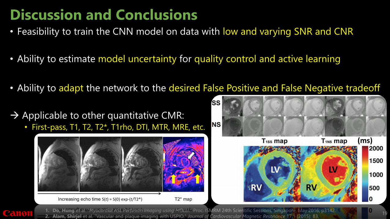
Discussion and Conclusions• Feasibility to train the CNN model on data with low and varying SNR and CNR

• Ability to estimate model uncertainty for quality control and active learning

• Ability to adapt the network to the desired False Positive and False Negative tradeoff

Applicable to other quantitative CMR: • First-pass, T1, T2, T2*, T1rho, DTI, MTR, MRE, etc.

191. Do, Hung et al. "Myocardial ASL Perfusion Imaging using MOLLI." Proc. ISMRM 24th Scientific Sessions, Singapore, May 2016, p3142.

2. Alam, Shirjel et al. "Vascular and plaque imaging with USPIO." Journal of Cardiovascular Magnetic Resonance 17.1 (2015): 83.

LV

RV

LV

RV

(ms)

Acknowledgements

• Funding:• Whittier Foundation

• NIH/NHLBI, #1R01HL130494-01A1

20

For over 100 years, the Canon Medical Systems `Made for Life’ philosophy prevails as our ongoing commitment

to humanity. Generations of inherited passion creates a legacy of medical innovation and service that

continues to evolve as we do. By engaging the brilliant minds of many, we continue to set the benchmark,

because we believe quality of life should be a given, not the exception.

Thank you for your attention!

Backup slides

77

49.537.4

22.914.4 12 10.1 9.65

16.5

0102030405060708090

1 2 4 8 16 32 64 128 256INFE

REN

CE

TIM

E (S

ECO

ND

)

BATCH SIZE

InferenceTime for 1024 MC trials

0

0.2

0.4

0.6

0.8

1 2 4 8 16 32 64 128 256MEA

N D

ICE

BATCH SIZE

Dice Mean

0

0.01

0.02

0.03

1 2 4 8 16 32 64 128 256

DIC

E ST

D

BATCH SIZE

Dice STD

Results(2): Uncertainty – Batch Size

23

Methods(3): dropout1

1. Srivastava et al., “Dropout: A simple way to prevent NN from overfitting.” JMLR 2014.

2. Animation is adapted from https://www.techemergence.com/what-is-machine-learning/24

Hidden Layer #1

HL #2 HL #3 HL #4

Output

Intro(3): Data characteristics of ASL

• Low SNR and contrast

1. Zungho Zun et al. “Assessment of myocardial blood flow in humans using arterial spin labeling: feasibility and SNR requirements.” MRM2009;62(4):975-83. 25

Control/Labeled Pulse Imaging

LV

RV

Methods(3): Uncertainty measure using MC dropout1

1. Gal, Yarin et al. "Dropout as a Bayesian approximation: Representing model uncertainty in deep learning." International conference on ML 2016; 1050-1059. 26

• Any NN, with dropout applied before every weight layer, is mathematically equivalent to an approximation of the Bayesian model.

• Model uncertainty can be estimated given the posterior distribution of the trained weights

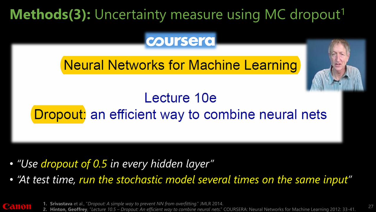
Methods(3): Uncertainty measure using MC dropout1

1. Srivastava et al., “Dropout: A simple way to prevent NN from overfitting.” JMLR 2014.

2. Hinton, Geoffrey, “Lecture 10.5 – Dropout: An efficient way to combine neural nets.” COURSERA: Neural Networks for Machine Learning 2012: 33-41. 27

• “Use dropout of 0.5 in every hidden layer”

• “At test time, run the stochastic model several times on the same input”

0.229 0.367 0.744 1.49 2.716

12

24

0

5

10

15

20

25

16 32 64 128 256 512 1024 2048INFE

REN

CE

TIM

E (S

ECO

ND

)

NUMBER OF MC TRIALS

Inference Time vs. # MC trials

Results(2): Uncertainty – Time penalty

1. Srivastava et al., “Dropout: A simple way to prevent NN from overfitting.” JMLR 2014. 28

~1.5s/image with 128 MC trials

Batch Size = 64

Figure 2: worst and best

29