NASA TECHNICAL NOTE N A S A TN D-4219

o*

N .d

v

n

1 DECOUPLING IN THE DESIGN AND SYNTHESIS OF MULTIVARIABLE CONTROL SYSTEMS

A. WOW& Etectlp.o&s Research Center Cambridge, Muss,

N A T I O N A L A E R O N A U T I C S A N D SPACE A D M I N I S T R A T I O N W A S H I N G T O N , D. C. OCTOBER 1967

https://ntrs.nasa.gov/search.jsp?R=19670030389 2018-07-04T19:40:56+00:00Z

i ,

~~ -

NASA T N D-4219

DECOUPLING IN THE DESIGN AND SYNTHESIS O F

MULTIVARIABLE CONTROL SYSTEMS

By Peter L. Fa lb and William A. Wolovich

Electronics Research Center Cambridge, Mass .

NATIONAL AERONAUTICS AND SPACE ADM IN I STRATI ON

For sale by the Clearinghouse for Federal Scientific and Technical Information Springfield, Virginia 22151 - CFSTl price $3.00

.

DECOUPLING IN THE DESIGN AND SYNTHESIS OF MULTIVARIABLE CONTROL SYSTEMS

By Peter L. Falb* and William A. Wolovich Electronics Research Center

SUMMARY

Necessary and sufficient conditions for the "decoupling" of an m-input,

m-output time-invariant linear system using state variable feedback are

determined. Given a system which satisfies these conditions, i. e. , which can

be decoupled by state variable feedback, the class CP of all feedback matrices

which decouple the system is characterized. The characterization of CP is used

to determine the number of closed loop poles which can be specified for the

decoupled system and to develop a synthesis technique for the realization of

desired closed loop pole configurations. Transfer matrix consequences of

decoupling are examined and practical implications discussed through numerical

examples.

1. INTRODUCTION

The development of techniques for the design of multivariable control

systems is of considerable practical importance. A particular design approach

involves the use of feedback to achieve closed loop control system stability. In

conjunction with this approach, it is often of interest to know whether or not it is

possible to have inputs control outputs independently, i. e., a single input influencing

a single output. This is, in heuristic terms, the problem of decoupling.

* Division of Applied Mathematics, Brown University, Providence, Rhode Island, and NASA Electronics Research Center, Cambridge, Massachusetts.

.

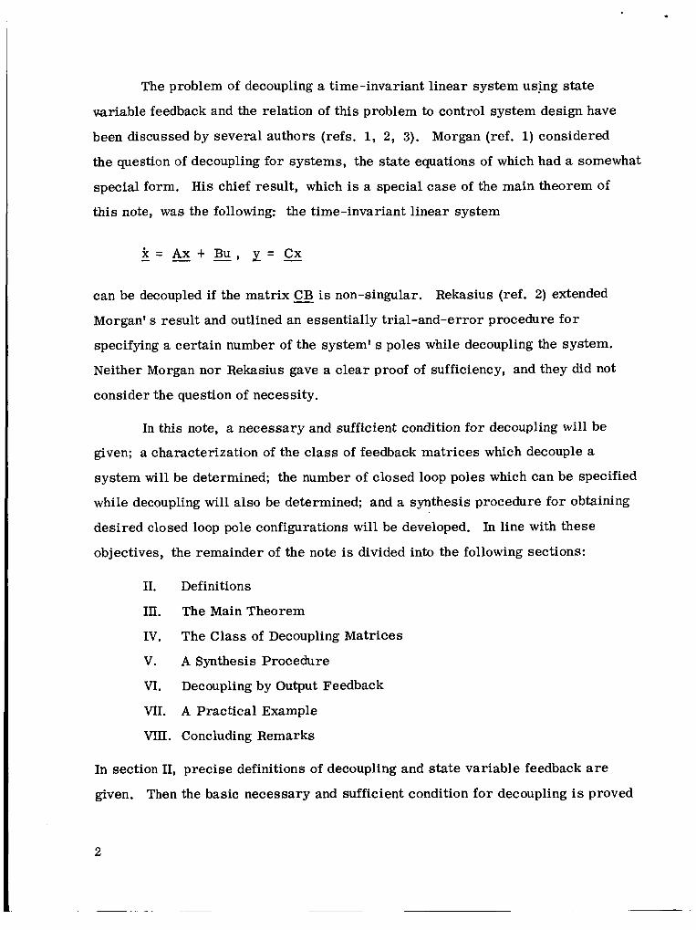
The problem of decoupling a time-invariant linear system us!ng state

variable feedback and the relation of this problem to control system design have

been discussed by several authors (refs. 1, 2, 3). Morgan (ref. 1) considered

the question of decoupling for systems, the state equations of which had a somewhat

special form. His chief result, which is a special case of the main theorem of

this note, was the following: the time-invariant linear system

can be decoupled if the matrix CB is non-singular. Rekasius (ref. 2) extended

Morgan' s result and outlined an essentially trial-and-error procedure for

specifying a certain number of the system' s poles while decoupling the system.

Neither Morgan nor Rekasius gave a clear proof of sufficiency, and they did not

consider the question of necessity.

In this note, a necessary and sufficient condition for decoupling will be

given; a characterization of the class of feedback matrices which decouple a

system wi l l be determined; the number of closed loop poles which can be specified

while decoupling will also be determined; and a synthesis procedure for obtaining

desired closed loop pole configurations will be developed. In line with these

objectives, the remainder of the note is divided into the following sections:

11.

ID. IV.

V.

VI.

VII.

VIII

Definitions

The Main Theorem

The Class of Decoupling Matrices

A Synthesis Procedure

Decoupling by Output Feedback

A Practical Example

Concluding Remarks

In section 11, precise definitions of decoupling and state variable feedback a r e

given. Then the basic necessary and sufficient condition for decoupling is proved

2

in section III. Using the main theorem, a description of all the decoupling matrices

l I

is presented (section IV). Next, the questions of synthesis and closed loop pole

placement a re examined (section V). In section VI, state variable feedback is

replaced by output feedback and the relevant theory developed. The practical poten-

tial of the methods is indicated in the discussion of a VSTOL stability augmentation

system in section VU. Finally, various concluding comments a r e made in

section VIII.

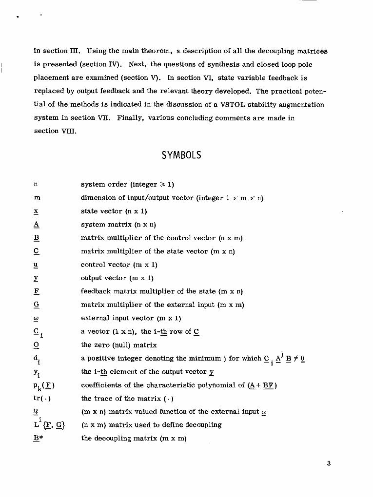
SYMBOLS

n

m

system order (integer >, 1)

dimension of input/output vector (integer 1 G m s n)

state vector (n x 1)

system matrix (n x n)

matrix multiplier of the control vector (n x m)

matrix multiplier of the state vector (m x n)

control vector (m x 1)

output vector (m x 1)

feedback matrix multiplier of the state (m x n)

matrix multiplier of the external input (m x m)

external input vector (m x 1)

a vector (1 x n), the i-t& row of C the zero (null) matrix

a positive integer denoting the minimum j for which C . A B # 0 the i-th - element of the output vector 1 coefficients of the characteristic polynomial of (A+ - BF)

the trace of the matrix ( . ) (m x n) matrix valued function of the external input - o (n x m) matrix used to define decoupling

the decoupling matrix (m x m)

j -1- -

3

det

F*, A*, G* - - -

E -i 6

M -k

S

9

H

-

- i

i s (E) E (E) - A**

K -

determinant (of a matrix)

(m x n), (m x n), and (m x m) matrices used in the proof of the decoupling theorem

(1 x n) row vector with 1 in the i-th - place and zeros elsewhere

positive integer = max d.

(m x m) diagonal matrices used in the synthesis of decoupling controllers

m x m diagonal matrix of differentiators

the class of all feedback matrices which decouple

(m x m) matrix multiplier of the output

(n x m) matrix used in the derivation of 9

(n x n) matrix used in the derivation of 9

(m x n) matrix used in the proof of the decoupling corollary

1

x n matrix involved with the synthesis question

1 1 . DEFINITIONS

Consider the time-invariant linear system

where 5 is an n vector called the state, 11 is an m vector called the control (or input),

is an m vector called the output, and A, E, C are n x n, n x m, and mxnmatr ices ,

respectively. It is assumed that m s n. If - F is an m x n matrix and G i s a non-

singular m x m matrix, then the substitution of

u = - - F x t w (2)

where - w represents the new m vector control (Fig. l), into (1) shall be called

linear state variable feedback.

4

Figure 1. Multivariable Feedback System

Let dl, d2 .... d be given by m

d. = min (1:C.A j B # 0 j = 0, 1, .. n-11, o r -1- - 2 1

j di = n - 1 if C . A B = 0 f o r a l l j -1-- -

where C . denotes the i-th - row of - C. Then, a simple calculation shows that - 1

di k = 0, 1, ..., k k C . ( A t BF) = -1- C . A 9 -1

k-di (4)

, k = d i t l ,...... n k di

C i ( A + E) = C . A ( A t E) -1- -

for i = 1, . . . , m. Application of the state variable feedback (2) and repeated

differentiation together with (4) yield the relations

yi = si& = C .(A t BF)x - 1 - -- .

di d . t 1

1 ( d i t 1)

= C . @ t B F ) x t C . ( A + = ) e -1 - - 'i -1

5

where y i' theorem,

i = 1, . . . , m, is the i-th - component of x. In view of the Cayley-Hamilton

n - 1

k = 0

where the pk( E) a re scalars depending upon E . Thus, - x can be eliminated from the

final relation of (5) to give

n - 1

where tr( . ) denotes the trace of a matrix, - Q is the m x n matrix given by

and Li{x, C+} is the n x m matrix given by

- - - Li{F, G} =

c . @ t E ) n - 1 - P n - l ( F ) @ t E ) n - 2 - . . . -p +l(F)@tFw)

c . @tE)n-2-Pn-l(F)@tBF)n-3-. . . -p t2(F)@+Ew)

BG

BG

-1 [ di I -1 [ di d!

C -i

0 -

(9)

i where 0 is a zero matrix consistent with the order of L {F, G} . If E .. denotes the

m x m matrix with 1 a s ij-g entry and zeros elsewhere, then E 52 is an m x n - 1J - - - -

-ii-

6

.

matrix with i-th row identical to the i-th row of Q and with all other rows zero. i

The matrix E .. D will be denoted by - Q . The following definition can now be made: - -

-11-

Definition.- The matrices --- F and G, -- with G nonsingular, decouple the system (1) - if

n - 1

k = 0

for i = 1, . . . . , m and if -

for i = 1, . . . , m. -

Note that this is a precise definition which does not involve vague statements about

inputs controlling outputs independently.

7

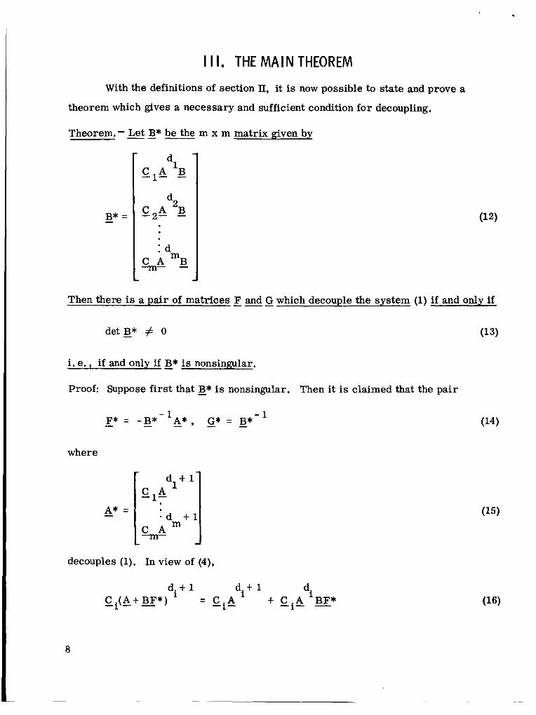
I 1 1 . THE MAIN THEOREM

With the definitions of section II, it is now possible to state and prove a

theorem which gives a necessary and sufficient condition for decoupling.

Theorem.- Let B* be the m x m matrix given by

dl

d2

C I A E

C A B -2-

: dm C A B -m- -

Then there is a pair of matrices --- F and G which decouple the system (1) if and only if

det - B* # 0 (13)

i. e . , if and only if - B* is nonsingular.

Proof: Suppose first that - B* is nonsingular. Then it is claimed that the pair

decouples (1). In view of (4),

di t Ci& E*

d.t 1 d i t 1 C . (A -t- BF*) 1 - - CiA -1 -

a

- - di But C .A B is simply ,the i-th row of B* , and so it follows that

-1- - d . t 1

-1 1 A* = -AT = - C . A -1- - - di

C i & BF* = -B*B* - 1- -

where Bf and A* are the i-th - rows of - B* and A* - respectively. Thus -1 -1

d. t k 1 = o -1 c .(& E*) -

for any positive integer k. In a similar way, it follows that

-1 - - di C. (A t BF*) BB*-l = B*B*-' - 1 - -

and hence that

- Li{ E*, g*}

- + I(F*)BTB*-' -1 - - 'd.

1

BTB*-' -1 -

- 1 However, B*B*

and so

= -i E ' a row vector with 1 in the i-th - place and zeros elsewhere, -1-

In other words, - F* and G* decouple (1).

9

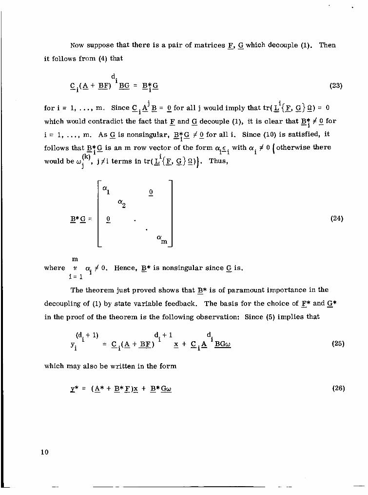
Now suppose that there is a pair of matrices - - F, G which decouple (1). Then

it follows from (4) that

di C . ( A t BF) = B*G -1 - - -1-

j for i = 1, . . . , m. Since CiA which would contradict the fact that - F and - G decouple (l), it is clear that ET # 0 for

i = 1, . . , , m. As G is nonsingular, B*G # 0 for all i. Since (10) is satisfied, it

follows that B*G is an m row vector of the form a x i with ai # 0 (otherwise there

would be u!~), j # i terms in tr( Li{& - G} E)). Thus,

= 0 for all j would imply that tr( - - - Li{F, G} 2) = 0

-1- - -

-1-

3

B*G = - -

m

1 a!

2 a!

0 -

0 -

Q! m

(24)

where 7r

i = 1

The theorem just proved shows that - B* is of paramount importance in the

ai # 0. Hence, - B* is nonsingular since - G is.

decoupling of (1) by state variable feedback. The basis for the choice of E* and G* in the proof of the theorem is the following observation: Since (5) implies that

which may also be written i n the form

y* = ( A * t B*F)x t B*Gw - - - - - -

10

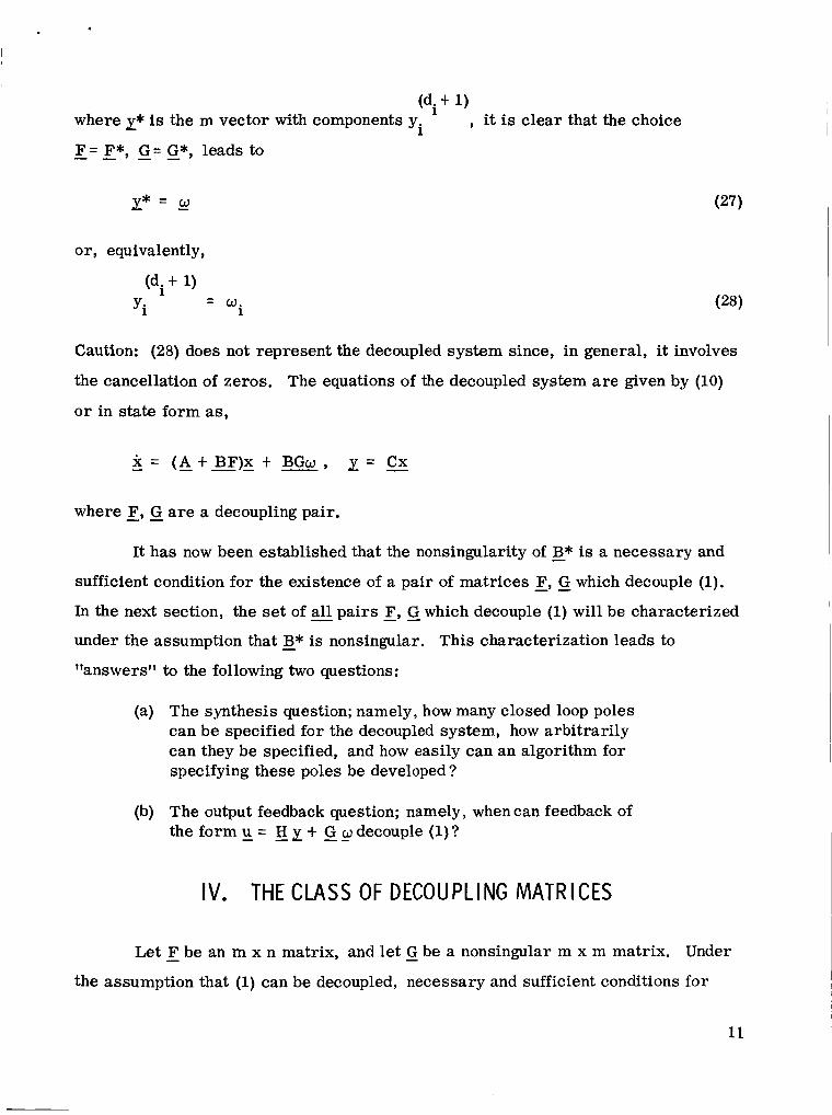
(d i t 1) where L* is the m vector with components y.

F = F*, G = G*, leads to

, it is clear that the choice 1

- - - -

y* = - 0

or, equivalently,

(d i t 1) = o (28 ) Y i i

Caution: (28) does not represent the decoupled system since, in general, it involves

the cancellation of zeros. The equations of the decoupled system a re given by (10)

o r in state form as,

where F, G a r e a decoupling pair. - -

It has now been established that the nonsingularity of - B* is a necessary and

sufficient condition for the existence of a pair of matrices E, G which decouple (1).

In the next section, the set of - all pairs - - F, G which decouple (1) will be characterized

under the assumption that - B* is nonsingular. This characterization leads to

"answersfr to the following two questions:

(a) The synthesis question; namely, how many closed loop poles can be specified for the decoupled system, how arbitrarily can they be specified, and how easily can an algorithm for specifying these poles be developed ?

(b) The output feedback question; namely, when can feedback of the form u - - = H 1 t -- G w decouple (l)?

IV. THE CLASS OF DECOUPLING MATRICES

Let - F be an m x n matrix, and let - G be a nonsingular m x m matrix. Under

the assumption that (1) can be decoupled, necessary and sufficient conditions for

11

- - F, G to be a decoupling pair are determined in this section. These conditions

turn out to be independent of G so that it will make sense to speak of the class a of matrices E which "decouple" (1).

Definition. - Let 9 (E) i be the n x m matrix given by

I- -

1 0 -

i - for i = 1, . . . , m, where 0 is a zero matrix consistent with the order of 9 (E). Let P (9, for i = 1, . . . , m, be the n x n matrix given by

i -- -

0 1

. .. 1 I 0

0 - I 1 I - I -

where the p ( F ) are the coefficients of the characteristic polynomial of

i.e., :

t x, k -

n - 1 k

( A - - t B F ) ~ = Pk(F)( j i -t E) 0

i -- and I i s an identity matrix consistent with the order of - - P ( F).

1 2

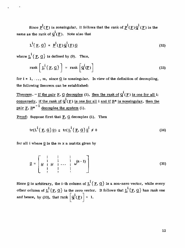
i i i Since (E) is nonsingular, it follows that the rank of .E (E) Q (I?) is the

i same as the rank of Q (I?). Note also that

where - Li{ E, 5) is defined by (9). Thus,

rank [ gi{ I?, G} ] = rank [Qi(F)] (33)

for i = 1, . . . , m, since - G is nonsingular. In view of the definition of decoupling,

the following theorem can be established:

Theorem. - If the pair I?, - G decouples (l), then the rank of Q ( - F ) is one for all i;

conversely, if the rank of 9 (3) is one for all i -- and if B* is nonsingular, then the

pair -9 F - B* - I, decouples the system (1).

i

i

Proof: Suppose first that - - F, G decouples (1). Then

for all i where - 52 is the m x n matrix given by

I I I I 1 I (n- 1)

_w I _w I * * * I W I I I I I I

(35)

i Since J z is arbitrary, the i-th column of - L {E, G} is a non-zero vector, while every

i other column of - Li (I?, G} is the zero vector. It follows that - L { - - F, G} has rank one

and hence, by (33), that rank

13

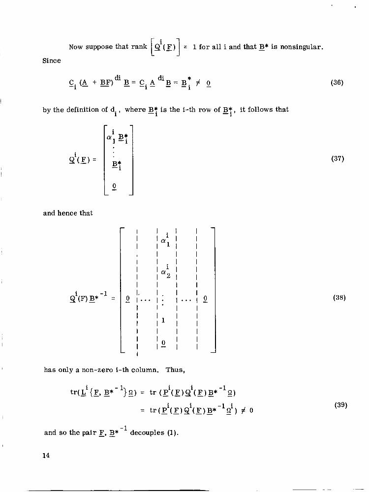
Now suppose that rank Q (E) = 1 for all i and that E* is nonsingular. F i 1 Since

di B = C . A d i B = B i * # 0 -1- - - c. (A, + BF) -

-1

by the definition of d. where B* is the i-th row of B*, it follows that 1 ' -1 - 1

i 9 ( E ) =

and hence that

I I I I I I I

I llyl I I I I I I I I I I I I

i I I 1"2 I I

I I I I

I 1 . I I I I

I I

I I I I I

I 1 I

I I I I l o I I

has only a non-zero i-th column. Thus,

(37)

and so the pa i r - - F, B*-l decouples (1).

14

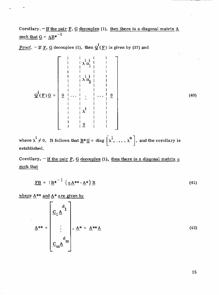
Corollary. - If the pair - - F, G decouples (l), then there is a diagonal matrix & such that - - G = AB*-’

Proof. - If - - F, G decouples (l), then 9 (E) is given by (37) and i

F ) G = - -

- 1 I I I I I A’; I I I I 11 I I I I I I I i i I I

I I I I I I I I

I P Q i I I

I I I I I I i I I I I A I I I I I I

I I I l o I - I I I

r .

and the corollary is 1’ i where A # 0. It follows that g*G = diag

established.

A , . . . ,

Corollary. - If the pair - - F, G decouples (l), then there is a diagonal matrix TJ

such that

where A** and A* are given by -- --

d

3-

, A_* = A**A - -

15

Proof. - The corollary is an immediate consequence of the relations

d. t 1 BFB 1 - di

d . t 1 1 = C . A B t C . A

-1- - -1- C . ( A t BF) - 1 - -

di d . t 1

1 C . (A t BF) = YiCi(A t BF) E - 1 - -

(43)

(44)

In summary, thus far it has been shown that the nonsingularity of E* is a

necessary and sufficient condition for the existence of a decoupling pair E, G. Furthermore, the set of all pairs E, G which decouple (1) consists of matrices E such that rank [gi(l?)l = 1 for all i and G such that - - G = AB*-' where is diagonal

L and nonsingular.

EXAMPLE: Let

J

In order to clarify these points, an example will now be presented.

1 0

2 0

1 3

7

1

B = -1 I 0 - :], - c =

0

0 0

0 1

(45)

Thus, - B* is nonsingular, and the system can be decoupled. The set

decouple the system (45) can now be obtained by determining all 2 x 3 matrices E of all - F which

16

such that rank r i d ’ Q ( F ) I = 1. In this example, this implies that the elements of + L .J

must be of the form:

f12

-f12- 1

V. A SYNTHES I S PROCEDURE

(47 1

The theorem presented in section IV does provide a procedure for determining

a, the class of all feedback matrices E which decouple (1). However, the direct

application of the condition, rank Q ( F ) = 1 for all i, results only in constraints

being placed upon certain of the m n parameters of E. What is still required is a

procedure for specifying closed loop system poles while simultaneously decoupling

(1) using an appropriate - F E +. In this light, a synthesis procedure will now be

presented for directly obtaining a feedback matrix E E +, the parameters of which

are determined so as to yield desired closed loop pole structure.

[ i - l

In particular, suppose that M k = 0, 1, 6 are given m x m matrices, then -k’

the choice

- - F = l3*-’[ -k- M CAk-A*] , = (48)

will, by (26), lead to

6 k

-k- M CA - x t g

k = 0

(49)

17

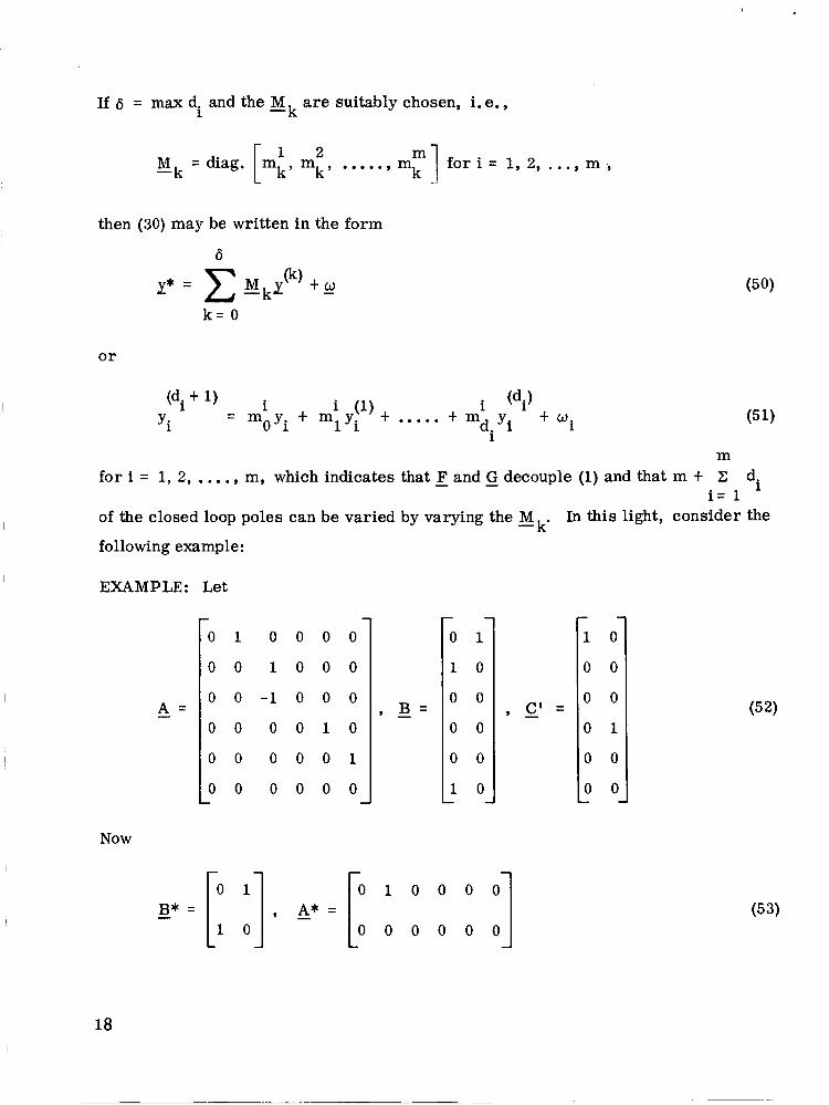
If 6 = max d. and the M a re suitably chosen, i. e., 1 -k

1 2 [ k , k , ....., mm] f o r i = 1 , 2 , ..., m , M = diag. m m k -k

then (30) may be written in the form

6

k = 0

o r

(di) (51)

i ..... t m y t wi d. i i (1) t (d i t 1) i

'i = moYi -I- mlYi 1

m for i = 1, 2, . . . . , m, which indicates that - F and - G decouple (1) and that m t 2

i = 1 of the closed loop poles can be varied by varying the M

following example:

EXAMPLE: Let

di

In this light, consider the - k'

A = -

0 1 0 0 0 0

0 0 1 0 0 0

0 0 - 1 0 0 0

0 0 0 0 1 0

0 0 0 0 0 1

0 0 0 0 0 0

0 1

1 0

0 0

0 0

0 0

1 0 -

- I 0 1 0 0 0 0

0 0 0 0 0 0

, g =

1 0

0 0

0 0

0 1

0 0

0 0 -

(53)

18

Since B* is nonsingular, the system can be decoupled. Setting, for example,

- M o = -1 M = M -2 =I: 11 (54) L -1

l one obtains, using (29), the decoupled system

2 3 2 Note that in this case det(s1 - A - - - BF) = s ( s t l)(s - s - s - l), where the poles 2 representing s(s3 - s - s - 1) have been specified by the choice of the M Other

choices of the M would lead to other closed loop pole configurations. Therefore,

i f E* is nonsingular, m t

specified (d. t 1 at a time) while simultaneously decoupling the system using the

synthesis procedure. The synthesis question is, therefore, partially resolved,

although some points still require clarification. In particular, it will be shown that

m -t Z d. can never exceed n, the number of system poles, and that it is sometimes

possible to specify more than m t 2 d. while simultaneously decoupling the system.

-k'

-k m d. of the system' s closed loop poles can be arbitrarily

1 1

1

m

1 1 m

1 ' m \

Lemma. - Let K be the xn matrix given by ---

.

19

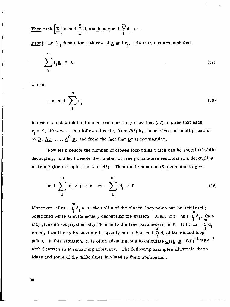
m m and hence m t T: d. s n .

1 ’

Proof: Let k . denote the i-th row of K and r arbitrary scalars such that i’ - -1

V

r k = O c i-i 1

where

m

di v = m t

1

(57)

In order to establish the lemma, one need only show that (57) implies that each

r. = 0. However, this follows directly from (57) by successive post multiplication

by - - B, AB, . . . , 4 - B, and from the fact that - B* is nonsingular. 6 1

Now let p denote the number of closed loop poles which can be specified while

decoupling, and let f denote the number of free parameters (entries) in a decoupling

matrix - F (for example, f = 3 in (47). Then the lemma and (51) combine to give

m m

m t x d i s p s n , m t x d i s f

1 1

(59)

m

1 ’ m Moreover, if m t Z d. = n, then all n of the closed-loop poles can be arbitrarily

positioned while simultaneously decoupling the system. Also, if f = m t Z di, then 1 m

(51) gives direct physical significance to the free parameters in F. If f > m t Z di m 1

(or n), then i t may be possible to specify more than m t Z d. of the closed loop

poles. In this situation, it is often advantageous to calculate - - C(sI-&-BF) E* with f entries in - F remaining arbitrary. The following examples illustrate these

ideas and some of the difficulties involved in their application.

1 ’ -1 -1

20

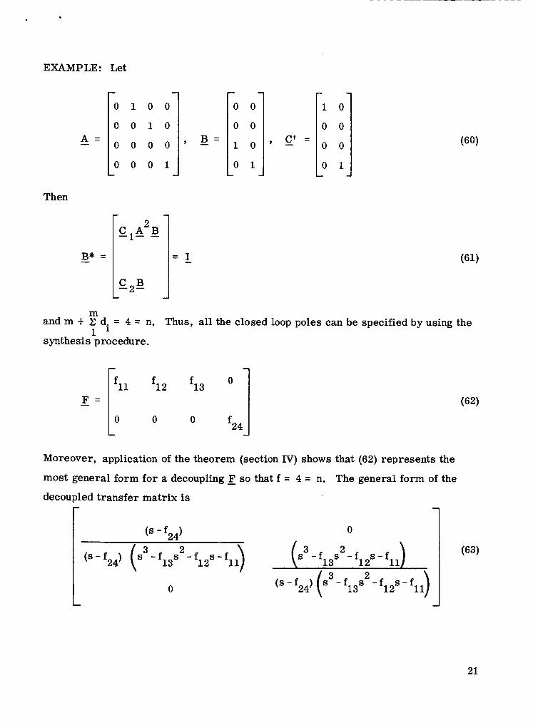
EXAMPLE: Let

A = -

Then

0 1 0 0 0 0

O 0 0 0 0

0 0 0 1 0 1

= I -

C B -2-

, c'= 0 0

0 1 1 :I m

and m t I: d. = 4 = n. Thus, all the closed loop poles can be specified by using the - 1 1

synthesis procedure.

- F = fll

0 -

f12

0

13

0 O I 24

Moreover, application of the theorem (section IV) shows that (62) represents the

most general form for a decoupling - F so that f = 4 = n. The general form of the

decoupled transfer matrix is

r (S - f24)

(s-f24) s - f s 2 -f12s-fll) ( 3 13

0

0

3 2 s - f s - f s-f

24 ( 3 13

13 1 2 11 2

(S- f ) s - f s

21

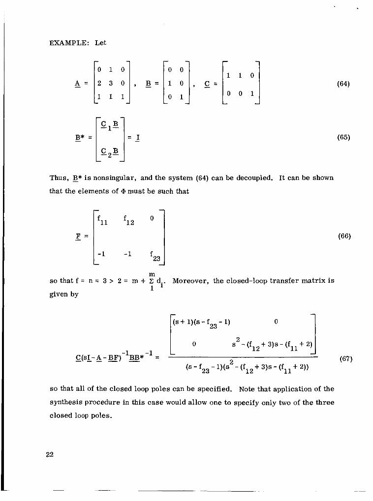
EXAMPLE: Let

Thus, - B* is nonsingular, and the system (64) can be decoupled. It can be shown

that the elements of 9 must be such that

f12

-1 ^I 23

m so that f = n = 3 > 2 = m t

given by

d.. Moreover, the closed-loop transfer matrix is 1 '

s t l)(s - f23 - 1) i; 0 1 s2 - (f t 3)s - (fll t 2)

(67) 1 2 J - - - C(SI - A - - ~ ~ ) - l g g * - l = l o

r) . . (s - f - l)(s" - (f t 3)s - (f t 2))

23 1 2 11

so that all of the closed loop poles can be specified. Note that application of the

synthesis procedure in this case would allow one to specify only two of the three

closed loop poles.

22

VI. DECOUPLING BY OUTPUT FEEDBACK

Since output feedback is only a special case of state variable feedback, i. e. :

with - HC replacing - F, it follows immediately that (1) can be decoupled using output

feedback if, and only if, (a) B* is nonsingular and (b) there is an m x m matrix H

such that rank Q (HC)

suitable test of whether or not a system can be decoupled using output feedback.

- - = 1 for i = 1, . . . , m. These conditions provide a [ i - l

EXAMPLE: Let

Then

- B* = [-: :] - l -1 l], 1 .=[' 0 0 1 O O]

0 0

is nonsingular so that the system defined by (69) can be decoupled. However, it is

- not possible to decouple this system using output feedback. To see this, observe

that the theorem and (39) imply that an - F which decouples must be of the form

F = - f12

-f -1 12 13 -f

23

*

and that - HC must be of the form

HC = -

L

0

0 h22 ”’’ Equations (71) and (72) lead to the contradictory requirement that f12 = 0 and

= - 1. This example illustrates the point that decoupling by state variable f12 feedback need not imply decoupling by output feedback.

It should be noted that although a system may be decoupled using output

feedback, some of the flexibility of specifying closed loop poles, as with state

variable feedback, will in general be lost. For example, consider the system

described by (60), with the most general - H given by

h22 O l

3 Since det(s1-A-BHC) = { d - l - h )(s - 22 - - -

(73)

), output feedback will not be adequate 11

to stabilize the system, although state variable feedback does provide a higher

degree of flexibility (63).

EXAMPLE: Consider the system described by (64). It has been shown (67) that

state variable feedback can be used to decouple the system while simultaneously

specifying all three closed loop poles. Application of the theorem (section IV) and

(39) imply that any 2 x 2 matrix - H of the form

H - h22 O I

(74)

24

.

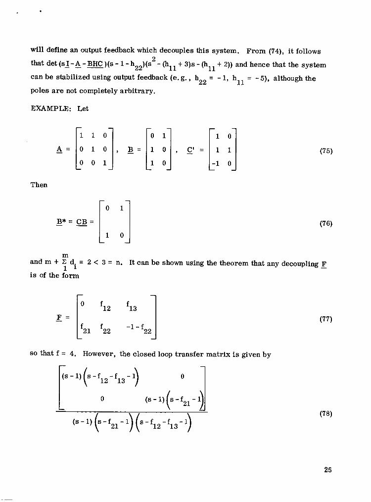
will define an output feedback which decouples this system. From (74), it follows

that det (s I -A - BHC )(s - 1 - h )(s - (hll t 3)s - (h 22 11 can be stabilized using output feedback (e. g., h22 = - 1, hll = - 5), although the

poles are not completely arbitrary.

2 t 2)) and hence that the system - - -

EXAMPLE: Let

-1 0

Then

(75)

- B * = C B = - [: :] (76)

m

1 1 and m t d. = 2 < 3 = n. It can be shown using the theorem that any decoupling F - is of the form

22 - 1 - f

so that f = 4. However, the closed loop transfer matrix is given by

(s-1)(8-f21-l)(s-f12-f13 -

(77)

25

so that p = 2; i. e., only two of the closed loop poles can be specified. It can also

be shown for this example that output feedback leads to the transfer matrix

- 1) (s - h12 - 1)

0

O 1

(s - I) (s -hZ1 - 4 (s-1) s - h 1 2 - 1 S-hZ1- ( )(

(79)

so that output and state variable feedback a r e equivalent. A s previous examples

illustrate, this is not true in general.

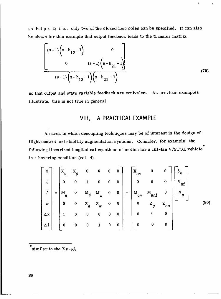
V I 1. A PRACTICAL EXAMPLE

An area in which decoupling techniques may be of interest is the design of

flight control and stability augmentation systems. Consider, for example, the

following linearized longitudinal equations of motion for a lift-fan V/STOL vehicle

in a hovering condition (ref. 4).

*

. . u

B

FJ

w

AX

Ai

'u xe 0 0

M O

0 0

1 0

0 0

U

0 0

1 0

M M

Z

e ' w

'e w

0 0

0 1

- 0

0

0

0

0

0 -

+

0 0

0 0 0

0

cv X

Mcv Mmf

'e C Z 0

0 0 0

0 0 0 -

* similar to the XV-5A

where the quantities are:

u - incremental longitudinal (x) velocity change

8 - incremental pitch angle

e' - pitch rate

w - incremental vertical (z) velocity change

Ax - incremental position e r ror

Az - incremental altitude e r ro r

- incremental collective fan input 6 V

- incremental nose fan input

- incremental fan stagger input

nf

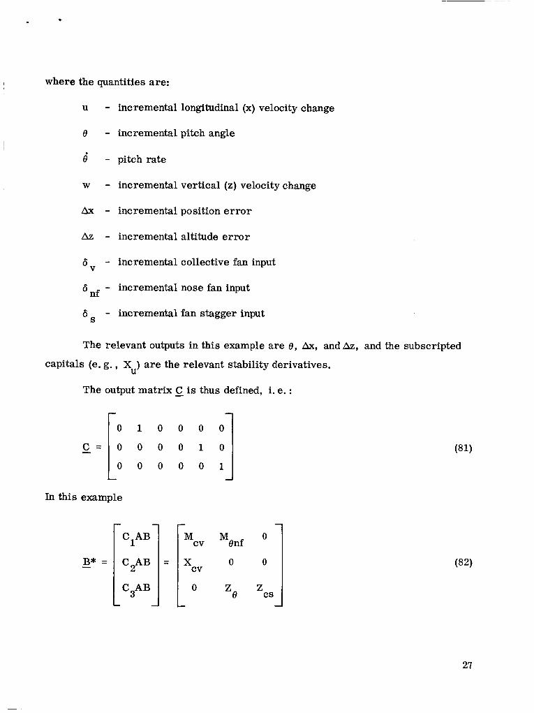
The relevant outputs in this example are e, Ax, and Az, and the subscripted

capitals (e. g. , X ) are the relevant stability derivatives. U

The output matrix C is thus defined, i. e. : -

0 0 0 0

In this example

27

3 and is nonsingular since it is assumed that Z

and hence all six of the closed-loop poles can be arbitrarily specified while simul-

taneously decoupling this system. It can be shown using the theorem that a decoupling

- F has 6 (i. e., f = 6) free parameters. Thus, the synthesis procedure (section V)

can be directly applied to give physical significance to these free parameters. For

example, suppose that independent pitch, translation, and altitude control are

desired, i. e. :

M X # 0. Therefore, m t Z d. = 6, 1 ’ cs enf cv

0 1 . ; = m e t m e t o 1 1 1

(83) 0 1 A S = m A x t m A k t w 2 2 2

0 1 A ~ = m A z t m A % t w 3 3 3

According to the synthesis procedure, - F can be set equal to B*-l - It can be shown that for this decoupling - F

A t B F = - -

28

1 2

m

0

0

0

1

0

0 0 0

0 1 0

l o 0

1 m 1 m

1 3

0 O m

0 0 0

0 0 1

0

2 m

0

0

0

0

0

0

0

0

0

3 m

0

0

-1 If - G is now set equal to E* , the closed-loop transfer matrix is:

2 1 - m s-m;)(s 2 1 -m3s-mo) 0 ,

0, (s 2 1 - m l s - m o ) ( s 2 - m j s - m ~ ) ,

0 , (s2- m t s - mo) 1 (s2- m i s -

2 1 - m s -m0)k2 - m1 - m0)k2 - m3s - m (85)

2 3 '

1

0 ,

1 1 2 2

- c(s I-A-BF)-~BB*-~ =

i J

If the m. are suitably chosen, then, in effect, the pilot will be faced with the task of

controlling three highly stable second-order systems. This example serves only to

indicate a potential practical area of application for the ideas presented in this paper.

The above examples illustrate the techniques developed for synthesizing

decoupling controllers for multivariable systems.

V I 1 1 . CONCLUDING REMARKS

The problem of decoupling a time-invariant linear system using state variable

feedback has been considered. Necessary and sufficient conditions for "decoup1ingvf

have been determined in terms of the nonsingularity of a matrix - B*. The class of

all feedback matrices which decouple a system has been characterized, and a

synthesis technique for the realization of desired closed loop pole configurations

has been developed. In essence, the major theoretical questions relating to

decoupling via state variable feedback have been resolved for time-invariant linear

systems.

A number of interesting potential areas of future research ar ise from the

results obtained here. In particular, the question of extending the theory to the

29

time-varying situation is of considerable interest. Some preliminary results

relating to stabilization have already been obtained.

VSTOL stability augmentation systems via decoupling techniques is a potential

practical area of application as was mentioned in section VII. Practical imple-

mentation of the techniques presented in this note has begun, but much remains to

be done before the theory is transformed into a practical design technique.

* The design of aircraft and

REFERENCES

1. Morgan, B. S. : The Synthesis of Linear Multivariable Systems by State

Variable Feedback. 1964 JACC, Stanford, California, pp. 468-472.

2. Rekasius, Z. V. : Decoupling of Multivariable Systems by Means of State

Variable Feedback. Third Allerton Conf. , 1965, Monticello, Illinois,

pp. 439-447.

3. Falb, P. L. and Wolovich, W. A. : On the Decoupling of Multivariable Systems.

1967 JACC, Philadelphia, Pennsylvania.

4. Seckel, E. : Stability and Control of Airplanes and Helicopters. Academic

Press, New York, 1964.

Electronics Research Center National Aeronautics and Space Administration

Cambridge, Massachusetts, August 1967 125-19-01 -01

* Wolovich, W .A. : On the Stabilization of Controllable Systems, NASA-ERC, Cambridge, Mass., 1967.

"The aeronautical and space activities of the United States shall be conducted so us to contribute . . . to the expansion of human know/- edge of phenomena in the atmosphere and space. The Admihistration &all provide for the widest practicuble and appropriate dissemination of information concerning its activities and the r e d s tbereof."

-NATIONAL AERONAU'ncs AND SPACE ACT OF 1958

NASA SCIENTIFIC AND TECHNICAL PUBLICATIONS

TECHNICAL REPORTS: Scientific and technical information considered important, complete, and a lasting contribution to existing knowldge.

TECHNICAL NOTES: Information less broad in scope but nevertheless of importance as a contribution to existing knowledge.

TECHNICAL MEMORANDUMS: Information receiving limited distribu- tion because of preliminary data, security classification, or other reasons.

CONTRACTOR REPORTS: Scientific and technical information generated under a NASA contract or grant and considered an important contribution to existing knowledge.

TECHNICAL TRANSLATIONS: Information published in a foEip language considered to merit NASA distribution in English.

SPECIAL PUBLICATIONS: Information derived from or of value to NASA activities. Publications include conference proceedings, monographs, data compilations, handbooks, sourcebooks, and special bibliographies.

TECHNOLOGY UTILIZATION PUBLICATIONS: Information on tech- nology used by NASA that may be of particular interest in commercial and other non-aerospace applications. Publications include Tech Briefs, Technology Utilization Reports and Notes, and Technology Surveys.

Details on the availability of these publications may be obtained horn:

SCIENTIFIC AND TECHNICAL INFORMATION DIVISION

N AT1 0 N A L A E R 0 N A UTI CS A N D SPACE AD M I N I ST R AT IO N

Washington, D.C. PO546